Stochastic Response Analysis of the Maglev Vehicle–Bridge Coupled System Considering Uncertain Parameters

Abstract

Previous studies on maglev vehicle–bridge coupled systems have mostly described the bridge using classical boundary conditions, while the effects of general constrained boundaries and uncertain parameters have not been fully considered. In this study, an energy-based dynamic model of a maglev vehicle–bridge coupled system is established. The boundary constraints of the bridge are introduced through equivalent springs, so that complex boundary conditions can be represented in a unified form. The proposed model is verified by comparison with published results. On this basis, Monte Carlo simulations are carried out to investigate the effects of random suspension parameters and random control parameters on the dynamic responses of the system. Two simplified electromagnetic-force models are also considered, and Sobol sensitivity analysis is used to evaluate the contributions of different parameters to the vibration responses and vibration energy. The results indicate that the suspension and control parameters affect different response quantities in different ways. The two electromagnetic-force models also lead to different sensitivity results, especially when the vibration energy is used as the evaluation index. The proposed method provides a useful tool for analyzing the stochastic vibration mechanism and optimizing the parameters of maglev vehicle–bridge coupled systems under general constrained boundaries.

1. Introduction

Maglev trains achieve contactless levitation and propulsion through electromagnetic force. Compared with wheel-rail trains, maglev trains do not come into contact with the ground during operation, which significantly reduces the frictional resistance. Thanks to its advantages, such as high running speed, low noise, and low maintenance cost, maglev trains have become an important development direction of high-speed railways [1]. Therefore, it is necessary to investigate the vibration characteristics of the maglev vehicle–bridge coupled system to ensure acceptable dynamic performance and running safety [2].

Many scholars have carried out relevant research on the dynamic modeling and vibration analysis of the maglev vehicle–bridge coupled system. Wang et al. [3] developed a vector-mechanics-based dynamic model for the maglev vehicle–bridge coupled system considering controller–rail–bridge interaction. Mao et al. [4,5] developed PDEM-based stochastic vibration models for the high-speed maglev vehicle–bridge coupled system and analyzed the effects of suspension parameters, bridge span, track irregularities, and running speed on running safety and stochastic dynamic responses. Huang et al. [6,7] established numerical models for the low–medium-speed maglev vehicle–bridge coupled system and investigated the effects of guideway irregularity, bridge dynamic characteristics, vehicle speed, and isolated bridge conditions on the coupled vibration responses. Liu and Guo [8] proposed a method to enhance the computational efficiency of the random vibration analysis for the maglev vehicle–bridge coupled system, which can effectively acquire the dynamic response and power spectral density of the maglev vehicle–bridge coupled system. Song et al. [9] established a maglev vehicle–bridge coupled system based on an elastic beam and investigated the influences of beam stiffness and vehicle load on the dynamic performance of the maglev system. Wang et al. [10] established a model of the maglev vehicle–bridge coupled system using simulation software and conducted a simulation analysis of the vertical dynamics of bridges under different span lengths and different operation speeds. Deng et al. [11] studied the influences of different working conditions on the ride comfort of maglev vehicles. Hu et al. [12] conducted research on the coupling vibration of the maglev vehicle–bridge coupled system and obtained the relationships between the vertical vibration amplitude at the mid-span of the bridge, the variation range of the suspension gap, and the vehicle speed. Zhang and Yu [13] adopted the Monte Carlo method and discussed the influences of speed, random irregularities, and random vehicle loads on the dynamic vibration of the maglev vehicle–bridge coupled system. Through comparing multiple results, such as the mean value time-history curves, probability density functions, and extreme value cumulative distribution functions, Wang et al. [14] analyzed the variation law of the dynamic reliability with the speed of the maglev train. Feng et al. [15] analyzed the influence laws of the operation speed and control parameters on the dynamic response under the effect of time delay. Selecting appropriate control parameters to reduce the influence of time delay is helpful for reducing the strong coupling vibration of the maglev vehicle–bridge coupled system. Liu and Guo [16] analyzed the vibration mechanism of the EMS-type maglev vehicle on the long-span bridge with double lines, and it was shown that the vertical interaction plays a dominant role in the maglev vehicle–bridge coupled system. Liang et al. [17] studied the vibration responses of the simply supported box girder bridge-maglev train system at different vehicle speeds. Li et al. [18] constructed a coupling system of a high-speed maglev train and a flexible long-span continuous rigid frame bridge. The analysis shows that the rigid car body will resonate with the bridge at low speeds, which should be avoided during the design process. Zhang et al. [19] compared the influence of suspension form on the response of the levitation module, air gap fluctuations, current, and power consumption. Xu et al. [20] studied the lateral responses of the bridge when the maglev train is operating on a long-span continuous girder bridge at relatively high speeds, as well as the bridge responses during the operation of double-way trains, in order to ensure the safe operation of the maglev train. Chen et al. [21] studied the influence of track beams with different spans and different deflection span ratios on the vibration response of the coupled system, providing a reference for the design of the maglev line. Most models assume that the bridge is under classical boundary conditions, but they are unable to describe the vibration characteristics of the maglev vehicle–bridge coupled system under general constrained boundaries.

In practical engineering projects, the influence of random parameters on the coupling vibration of the maglev vehicle–bridge coupled system is extremely significant. Xia et al. [22] analyzed the influences that the parameters of the bridge and the controller have on the dynamics of the maglev system. Wen et al. [23] developed a three-dimensional elastic model with parameter uncertainty considered by combining the pseudo-excitation method (PEM) and the energy method. Sun et al. [24,25] analyzed the influence patterns of the control parameters in the maglev vehicle–guideway system and the stable range of the system to suppress the coupling vibration. It was also proposed to adjust the proportional gain parameter of the suspension control online to improve the dynamic performance of the system, enabling the maglev system to obtain a larger stable state range, thus effectively suppressing the vehicle-track interaction vibration. Talukdar [26] optimized the suspension parameters, which effectively reduced the vertical acceleration of the car body and the maximum deflection of the guideway. Yang et al. [27] further studied the phase deviation problem in semi-active suspension control and proposed an inertial-suspension-based compensation method. Their study indicated that suspension performance is closely related to both structural parameters and control strategy, which also highlights the importance of considering suspension and control parameters in dynamic response analysis. Wen et al. [28] developed a three-dimensional elastic vehicle model including suspended equipment based on the energy method, and investigated the effects of the suspension parameters of the suspended equipment on the stochastic vibration response of the vehicle. Zhou et al. [29] conducted a global sensitivity analysis on the stochastic response of rail vehicles with uncertain parameters and discussed the influence of uncertain suspension parameters on the stochastic vibration characteristics of the rail vehicle system. Chen et al. [30] adopted more optimal PID control parameters, which significantly improved the levitation stability of the maglev train under the action of random guideway irregularities. Zhou and Li [31] discussed the influences of different control parameters on the maglev vehicle–bridge coupled system, and demonstrated that appropriate control parameters can reduce the coupling vibration response. Wang et al. [32] introduced fuzzy active control, which reduced the overall response of the bridge and improved the comfort of the maglev train.

According to the above-mentioned literature, many researchers have carried out relevant studies on the vibration characteristics of the maglev vehicle–bridge coupled system, as well as the influence of bridge parameters and control parameters on the vibration response of the system. However, at present, there are few studies on the uncertain vibration analysis of the maglev vehicle–bridge coupled system from the perspective of the energy method, resulting in an unclear understanding of the vibration energy characteristics. At the same time, there are currently two simplified methods for electromagnetic force, and the influence of these two methods on the vibration response has not been investigated yet.

Therefore, the development of a maglev vehicle–bridge coupled system capable of considering random parameters is of substantial significance. Although a number of researchers have initiated relevant investigations, there currently exist the following inadequacies. Firstly, the majority of these studies employ classical boundaries to depict the bridge boundaries, thereby overlooking the impact of intricate boundary conditions. Secondly, most of them fail to take into account the influence of random suspension parameters and random control parameters on the vibration characteristics of the system [23,28].

The following work has been carried out in this paper:

(1)

A maglev vehicle–bridge coupled system under general constrained boundaries was established.

(2)

The influence of uncertain suspension parameters and control parameters on the response was discussed.

(3)

Sensitivity analyses were conducted on the models under two different control models.

2. Theoretical Modeling

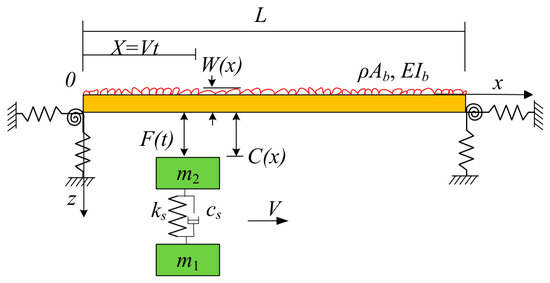
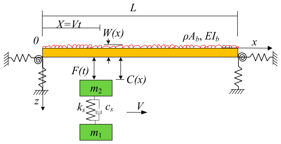
In this study, the calculation model of the two-degree-of-freedom vehicle with constant conductivity passing through the simply supported beam bridge at uniform speed is adopted, as shown in Figure 1. The vehicular system comprises three primary components: the car body, the car-body suspension system, and electromagnets. m₁ and m₂ are the mass of the car body and electromagnet, respectively, and k_s and c_s are the stiffness and damping of the car-body suspension, respectively. L is the bridge span, ρA_b and EI_b are the linear density and flexural stiffness of the bridge. It is assumed that the bridge deck maintains a horizontal configuration under its self-weight prior to the traversal of the maglev vehicle, and that no relative displacement occurs between the guideway and the bridge deck. Let w(x) denote the track irregularity random field, defined as positive downward, where the spatial coordinate x is parameterized by the vehicle’s traversal motion as x = Vt, with V being the constant velocity and t representing time.

2.1. Equation of Motion of Bridge System

Using the first-order shear deformation theory (FSDT), each displacement component of the bridge is expressed as [29]:

$$\begin{array}{l}U(x,t)=u(x,t)+z{\phi }_x(x,t)\\ W(x,t)=w(x,t)\end{array}$$

(1)

where u and w denote the middle plane displacements of the bridge in the x and z directions. φ_x is the cross-sectional rotation, and t is the time variable.

Based on the linear strain–displacement relation, the strains of the bridge are given by:

$$\left\{\begin{array}{l}{\epsilon }_x\\ {\gamma }_{xz}\end{array}\right\}=\left\{\begin{array}{l}{\displaystyle \frac{\partial u}{\partial x}}+z{\displaystyle \frac{\partial {\phi }_x}{\partial x}}\\ {\phi }_x+{\displaystyle \frac{\partial w}{\partial x}}\end{array}\right\}$$

(2)

The normal and shear stresses of the bridge can be further expressed as:

$$\left\{\begin{array}{l}{\sigma }_x\\ {\tau }_{xz}\end{array}\right\}=\left[\begin{array}{cc}E& 0\\ 0& kG\end{array}\right]\left\{\begin{array}{l}{\epsilon }_x\\ {\gamma }_{xz}\end{array}\right\}$$

(3)

where k is the shear correction factor, E is the elastic modulus, and G is the shear modulus.

The strain and kinetic energies of the bridge are expressed:

$$\begin{array}{l}{U}_v={\displaystyle {\int }_0^L{\displaystyle {\int }_{-h/2}^{h/2}{\displaystyle {\int }_{-b/2}^{b/2}\left\{\frac{1}{2}{\sigma }_x{\epsilon }_x+\frac{1}{2}{\tau }_{xz}{\gamma }_{xz}\right\}}}}dxdydz\\ T_v={\displaystyle {\int }_0^L{\displaystyle {\int }_{-h/2}^{h/2}{\displaystyle {\int }_{-b/2}^{b/2}\left\{\frac{1}{2}\rho {(\frac{\partial U}{\partial t})}^2+\frac{1}{2}\rho {(\frac{\partial W}{\partial t})}^2\right\}}}}dxdydz\end{array}$$

(4)

where ρ is the equivalent density of the bridge.

The equivalent elastic energy introduced by the constraints at both ends of the bridge can be expressed as:

$$\begin{array}{l}{U}_{BC}={\displaystyle \frac{1}{2}}\left[k_{ux0}{(u)}^2+k_{wx0}{(w)}^2+k_{xx0}{({\phi }_x)}^2\right]{|}_{x=0}+\\ {\displaystyle \frac{1}{2}}\left[k_{uxL}{(u)}^2+k_{wxL}{(w)}^2+k_{xxL}{({\phi }_x)}^2\right]{|}_{x=L}\end{array}$$

(5)

where k_ux0, k_wx0, and k_xx0 are the longitudinal spring stiffness, vertical spring stiffness, and rotational spring stiffness provided by the support at the left end of the bridge (x = 0), respectively; k_uxL, k_wxL, and k_xxL are the longitudinal spring stiffness, vertical spring stiffness, and rotational spring stiffness provided by the support at the right end of the bridge (x = L), respectively.

2.2. Vehicle System Motion Equation

The elastic and dissipated energies of the car-body suspension are expressed:

$$\begin{array}{l}{U}_p={\displaystyle \frac{1}{2}}{k}_s{\left(y_v(t)-y_m(t)\right)}^2\\ W_p=-{\displaystyle \frac{1}{2}}{c}_s{\left({\dot{y}}_v(t)-{\dot{y}}_m(t)\right)}^2\end{array}$$

(6)

where y_v(t) is the vertical displacement of the electromagnet and y_m(t) is the vertical displacement of the vehicle.

The sum of the kinetic energies of the car body and the suspension frame is expressed as:

$$T_b={\displaystyle \frac{1}{2}}{m}_1{({\dot{y}}_m)}^2+{\displaystyle \frac{1}{2}}{m}_2{({\dot{y}}_v)}^2$$

(7)

2.3. Equation of Electromagnetic Force

Unlike the wheel-rail direct contact method, maglev vehicles overcome gravity by means of the electromagnetic attraction between the electromagnet and the track to achieve suspension. Assuming that the magnetic permeability of the ferromagnetic material in the electromagnet magnetic circuit is infinite, and the magnetic potential is evenly distributed in the suspended air gap, and the leakage flux in the electromagnet winding is ignored, the instantaneous suction force generated by the loop electromagnet in the electromagnet winding can be expressed as [30]:

$$F(t)={\displaystyle \frac{{\mu }_0{N}^{2}A}{4}}{\left({\displaystyle \frac{I(t)}{c(x)}}\right)}^2$$

(8)

where µ₀ represents the air permeability, N is the number of turns of the electromagnet coil, A is the effective magnetic pole area, I(t) is the electromagnet current, and c(x) is the suspension gap.

Set the current and the suspension gap of the vehicle system during static suspension as I₀ and c₀, respectively. The electromagnetic force is equal to the gravity G of the vehicle system. The first-order Taylor expansion of the electromagnetic force is performed at the static suspension. The expression formula of the nonlinear electromagnetic force in Equation (8) can be expressed in a linear manner as:

$$F(t)=G+[k_I\Delta I(t)-k_c\Delta c(x)]$$

(9)

where ΔI(t) and Δc(x) are the variation of the current and the variation of the suspension gap, respectively. k_I and k_c are the corresponding proportionality coefficients, which can be expressed as:

$$\begin{array}{l}{k}_I={\displaystyle \frac{{\mu }_0{N}^{2}A{I}_0}{2c_0^2}}\\ k_c={\displaystyle \frac{{\mu }_0{N}^{2}A{I}_0^2}{2c_0^3}}\end{array}$$

(10)

The electromagnetic force serves as an active control input. By feeding signals such as levitation-gap variation into the levitation controller, the electromagnetic force can be dynamically adjusted. This closed-loop regulation enables effective control of the levitation-gap variation, thereby maintaining vehicle levitation stability. Select the variation of the suspension gap Δc(x), the vertical velocity ${\dot{y}}_v\left(t\right)$, and the vertical acceleration ${\ddot{y}}_v\left(t\right)$ of the vehicle electromagnet as the state feedback quantities, then the current control law can be expressed as:

$$\Delta I_1(t)=G_1\Delta c(x)+G_2{\dot{y}}_v(t)+G_3{\ddot{y}}_v(t)$$

(11)

where G₁, G₂, and G₃ are the feedback coefficients of Δc(x), ${\dot{y}}_v\left(t\right)$ and ${\ddot{y}}_v\left(t\right)$, respectively.

According to the geometric compatibility condition between the vehicle and the bridge, the variation of the suspension gap can be expressed as:

$$\Delta c(x)=y_v(t)-y_b(x,t)-w(x)$$

(12)

where $y_v\left(t\right)$ is the vertical displacement of the vehicle electromagnet; $y_b(x,t)$ is the vertical displacement of the bridge at the acting point of the electromagnetic force.

Substituting Equations (10)–(12) into Equation (9), the electromagnetic force can be expressed as:

$$F_1(t)=G+\left\{k_1\left[y_v(t)-y_b(x,t)-w(x)\right]+k_2{\dot{y}}_v(t)+k_3{\ddot{y}}_v(t)\right\}$$

(13)

where k₁, k₂, k₃ can be calculated:

$$\begin{array}{l}{k}_1=k_I{G}_1-k_c\\ k_2=k_I{G}_2\\ k_3=k_I{G}_3\end{array}$$

(14)

In addition, there is another commonly used control strategy. By selecting the variation of the levitation gap Δc(x) and the variation rate of the levitation gap Δ$\dot{c}$(x) as the state feedback quantities, the current control rate can be expressed as [33]:

$$\Delta I_2(t)=G_1\Delta c(x)+G_2\Delta \dot{c}(x)$$

(15)

where G₁ and G₂ are the feedback coefficients of Δc(x) and Δ$\dot{c}$(x), respectively. G₁ and G₂ are the same as the coefficients in Equation (11).

The electromagnetic force can be expressed as:

$$F_2(t)=G+\left\{k_1\left[y_v(t)-y_b(x,t)-w(x)\right]+k_2\left[{\dot{y}}_v(t)-{\dot{y}}_b(x,t)\right]\right\}$$

(16)

where k₁ and k₂ are the same as the values in Equation (14).

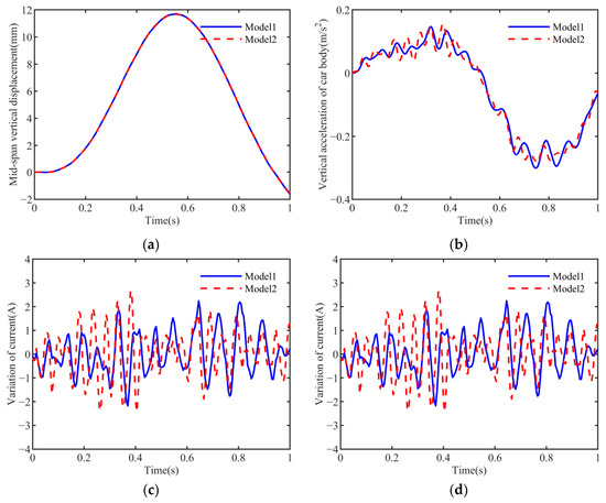
For convenience, the model based on the current control law in Equation (11) is referred to as Model 1, while the model based on the current control law in Equation (15) is referred to as Model 2. The two current control laws have different physical meanings. In Model 1, the levitation-gap variation, the absolute vertical velocity, and the absolute vertical acceleration of the vehicle electromagnet are selected as feedback quantities. Therefore, the electromagnetic force contains not only the equivalent stiffness term related to the levitation gap, but also the feedback terms associated with the absolute motion of the electromagnet. In contrast, Model 2 uses the levitation-gap variation and its variation rate as feedback quantities. This means that the electromagnetic force is mainly determined by the relative displacement and relative velocity between the electromagnet and the bridge. Therefore, Model 1 can be regarded as a control model with absolute motion feedback of the electromagnet, while Model 2 represents a relative levitation-gap feedback model. Although the two models have the same static equilibrium state, their dynamic feedback mechanisms are different, which may lead to different vibration responses, levitation-gap variations, and current variations.

2.4. Trial Functions and Unified Solutions

In the traditional method, the trial functions are different and quite complicated for different boundary conditions. In this paper, the unified trial functions are chosen based on the energy method. The modified Fourier series is adopted in this paper. The displacement components of the bridge can be expressed as:

$$\begin{array}{l}u(x)={\displaystyle \sum _{m=0}^{\infty }{A}_{mn}\cos ({\lambda }_{m}x)}+f_{1n}^1{\xi }_{1a}(x)+f_{2n}^1{\xi }_{2a}(x)\\ w(x)={\displaystyle \sum _{m=0}^{\infty }{B}_{mn}\cos ({\lambda }_{m}x)}+f_{1n}^2{\xi }_{1a}(x)+f_{2n}^2{\xi }_{2a}(x)\\ u(x)={\displaystyle \sum _{m=0}^{\infty }{C}_{mn}\cos ({\lambda }_{m}x)}+f_{1n}^3{\xi }_{1a}(x)+f_{2n}^3{\xi }_{2a}(x)\end{array}$$

(17)

where ${\lambda }_m=m\pi /L(m=\mathrm{0,1},\dots ,\mathrm{\infty })$, $A_{mn}$, $B_{mn}$ and $C_{mn}$ represent the Fourier series expansion coefficients. $f_{1n}^l$ and $f_{2n}^l(l=\mathrm{1,2},3)$ are the corresponding supplement coefficients.

In order to overcome the possible discontinuity problems on the boundary, the auxiliary functions can be expressed by:

$${\xi }_{1a}(x)=L{\displaystyle \frac{x}{L}}{({\displaystyle \frac{x}{L}}-1)}^2,{\xi }_{2a}(x)=L{({\displaystyle \frac{x}{L}})}^2({\displaystyle \frac{x}{L}}-1)$$

(18)

Then, the following relation can be obtained:

$$\begin{array}{l}{\xi }_{1a}(0)={\xi }_{1a}(L)={\xi }_{1a}^{\prime }(L),{\xi }_{1a}^{\prime }(0)=L\\ {\xi }_{2a}(0)={\xi }_{2a}(L)={\xi }_{2a}^{\prime }(L),{\xi }_{2a}^{\prime }(0)=L\end{array}$$

(19)

which means the first-order derivatives of the proposed trial functions are continuous at both ends of the bridge.

It is assumed that the infinite series terms in Equation (17) are uniformly truncated to M in actual calculations, and the energy expressions (1)–(7) are substituted into Hamilton’s principle:

$$\delta {\displaystyle {\int }_{t_0}^{t_1}(T_v+T_b-U_v-U_p-U_{BC}+W_p)}dt=0$$

(20)

3 × M + 8 linear algebraic equations can be obtained, which can be further expressed in the following matrix form:

$$\left[\begin{array}{cc}{M}_b& \\ & M_v\end{array}\right]\left[\begin{array}{c}{\ddot{Y}}_b\\ {\ddot{Y}}_v\end{array}\right]+\left[\begin{array}{cc}{C}_b& C_{bv}\\ C_{vb}& C_v\end{array}\right]\left[\begin{array}{c}{\dot{Y}}_b\\ {\dot{Y}}_v\end{array}\right]+\left[\begin{array}{cc}{K}_b& K_{bv}\\ K_{vb}& K_v\end{array}\right]\left[\begin{array}{c}{Y}_b\\ Y_v\end{array}\right]=\left[\begin{array}{c}{F}_i(t)\\ G-F_i(t)\end{array}\right],i=1,2$$

(21)

where subscript b denotes the bridge, M_b, C_b and K_b are the mass matrix, damping matrix and stiffness matrix of the bridge system, respectively; ${\mathbf{Y}}_b$, ${\dot{\mathbf{Y}}}_b$ and ${\ddot{\mathbf{Y}}}_b$ are the displacement vector, velocity vector and acceleration vector of the bridge system, respectively; subscript v denotes the vehicle, M_v, C_v and K_v are the mass matrix, damping matrix and stiffness matrix of the vehicle system, respectively, and stiffness matrix, respectively; ${\mathbf{Y}}_v$, ${\dot{\mathbf{Y}}}_v$, ${\ddot{\mathbf{Y}}}_v$ and are the displacement vector, velocity vector, and acceleration vector of the vehicle system, respectively; G is the gravity force of the vehicle system; and F_i(t) are the electromagnetic forces under different current control laws between the two models.

2.5. Sensitivity Analysis Method

The Sobol method is adopted in this study for global sensitivity analysis. Sobol sensitivity analysis is based on variance-decomposition theory. It does not require the model to be linear. The method only requires the input variables to be mutually independent and the model output to have a finite variance. This method defines a (k)-dimensional unit hypercube (Ω^k) as the input parameter space, which can be expressed as Ω^k = {x|0 ≤ x_i ≤ 1, i = 1, 2, …, k}. The core idea of the Sobol sensitivity analysis method is to decompose the function into a sum of component functions:

$$\begin{array}{l}f(x_1,x_2,\dots ,x_k)=f_0+{\displaystyle {\displaystyle \sum _i^k}{f}_i(x_i)}+{\displaystyle {\displaystyle \sum _{0\le i\le j\le k}^k}{f}_i(x_i)}\\ +\cdots +f_{1,2,\dots ,k}(x_1,x_2,\dots ,x_k)\end{array}$$

(22)

In the above equation, the right-hand side contains (2^k) component functions, and different decomposition forms can be used. A decomposition method based on multiple integration is usually adopted. According to the definition of continuous variance and basic statistical theory, the total variance of the model output (f(x)) is given by:

$$D={\displaystyle \int f^2(x)}dx-f_0^2$$

(23)

The variances of the component terms of (f(x)) at different orders are referred to as partial variances. Accordingly, the (s)-order partial variance is given by:

$$D_{i_1,i_2,\dots ,i_s}={\displaystyle {\displaystyle \underset{0}{\overset{1}{\int }}}\cdots {\displaystyle {\displaystyle \underset{0}{\overset{1}{\int }}}{f}_{i_1,i_2,\dots ,i_s}^2(x_{i_1},x_{i_2},\dots ,x_{i_s})d{x}_{i_1}d{x}_{i_2}\cdots d{x}_{i_s}}}$$

(24)

By squaring both sides of the decomposition of (f(x)) and integrating over the whole domain, and considering the mutual orthogonality of the component terms, it can be concluded that the total variance is equal to the sum of the partial variances at different orders. In addition, the sensitivity coefficient at each order is defined as the ratio of the corresponding partial variance to the total variance. In this study, the first-order sensitivity coefficient is mainly used to evaluate the influence of each parameter on the response.

Finally, to facilitate the calculation, the integrals can be estimated using the Monte Carlo method:

$${\overline{f}}_0={\displaystyle \frac{1}{n}}{\displaystyle \sum _m^{n}f(x_m)}$$

(25)

$$\overline{D}={\displaystyle \frac{1}{n}}{\displaystyle \sum _m^n{f}^2(x_m)}-{\overline{f}}_0^2$$

(26)

$${\overline{D}}_i={\displaystyle \frac{1}{n}}{\displaystyle \sum _m^{n}f(x_{im}^{(1)},x_{-\left(i\right)m}^{(1)})f(x_{im}^{(1)},x_{-\left(i\right)m}^{(2)})}-{\overline{f}}_0^2$$

(27)

In the equation, when (${\overline{D}}_i$) is calculated, two values of (f) are multiplied. One value of (f) is obtained by substituting the corresponding vector (x) from the first sample set. The other value of (f) is obtained by substituting a mixed vector, in which all components except (x_i) are taken from the second sample set, while (x_i) remains unchanged.

3. Model Verification

The maglev vehicle–bridge coupled model shown in Figure 1 was used to carry out numerical simulation research. Detailed parameters are listed in

Table 1. The specific parameters of the model.

Items	Notation	Value
car-body mass	m1	500 kg
electromagnet mass	m2	300 kg
car-body suspension stiffness	ks	1.4 × 104 N/m
car-body suspension damping	cs	5.8 × 102 N·s/m
air permeability	µ0	4π × 10−7 H/m
effective magnetic pole area	A	0.049 m2
coil turns	N	356 T
static suspended floating current	I0	20 A
static suspension gap	c0	0.01 m
displacement feedback coefficient	G1	7500 A/m
velocity feedback coefficient	G2	10 A·s/m
acceleration feedback coefficient	G3	0.5 A·s2/m
bridge span	L	20 m
linear density	ρAb	1.42 × 103 kg/m
flexural stiffness	EIb	1.66 × 108 N·m2

, which can be obtained from the literature [30].

The power spectral density function of orbital irregularity can be expressed as [33]:

$$S_w(\omega )={\displaystyle \frac{A_w}{{\omega }^{\alpha }}}$$

(28)

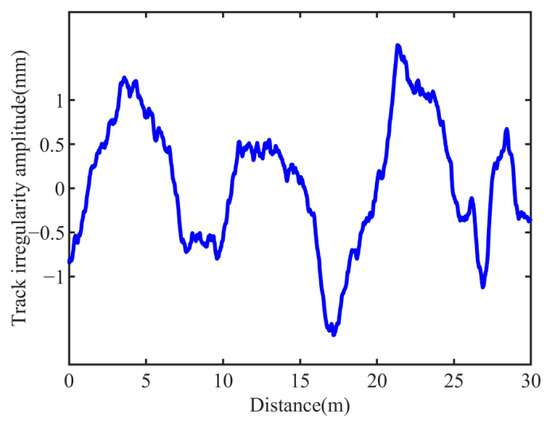
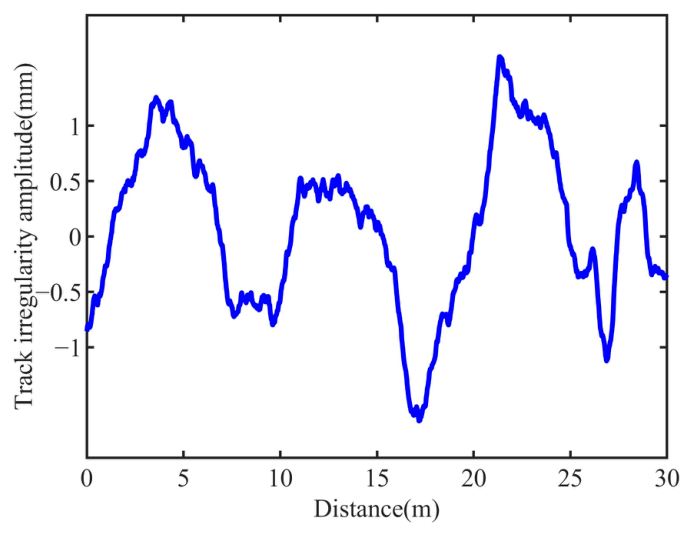
where ω is the spatial circular frequency, ω = 2πf, and f is the spatial frequency; α is the frequency characteristic parameter; A_ω is the roughness coefficient. α, A_ω, and f are three characteristic parameters that can be obtained from the literature [34]. The track irregularity samples generated by the calculations in this paper are shown in Figure 2.

3.1. Convergence Study

To determine the specific value of the truncation number M required for the bridge, this section conducts a relevant analysis on the convergence of the bridge’s natural frequencies with respect to the order M of the basis functions. As shown in

Table 2. Convergence analysis of natural frequencies (Hz) with respect to the truncation number (M).

Mode	M = 4	M = 6	M = 8	M = 10	M = 12	M = 14	M = 16
1	1.34	1.34	1.34	1.34	1.34	1.34	1.34
2	5.62	5.36	5.33	5.33	5.32	5.32	5.32
3	14.25	11.96	11.87	11.85	11.85	11.85	11.84
4	32.55	21.56	20.89	20.79	20.76	20.75	20.75
5	40.23	38.92	32.19	31.93	31.86	31.84	31.83
6	80.52	40.22	40.22	40.22	40.22	40.22	40.22
7	124.36	72.57	46.34	45.17	44.97	44.91	44.88
8	167.67	80.46	72.70	60.33	59.85	59.73	59.70

, it can be observed that when the order M > 12, the natural frequencies of the bridge system exhibit good convergence. Therefore, in subsequent numerical examples, the order M of the bridge’s basis functions is set to 14.

3.2. Verification of the Correctness of the Model

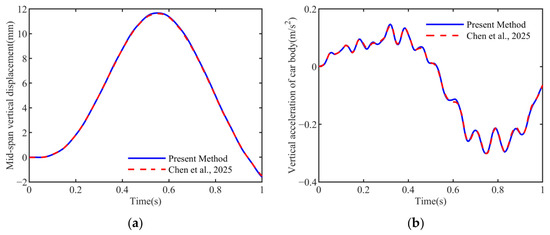
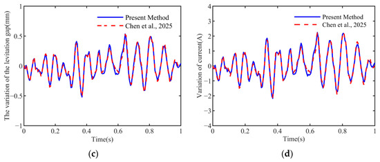
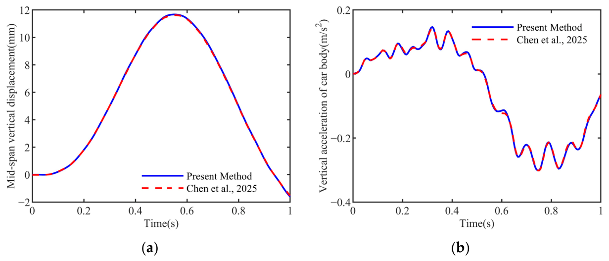
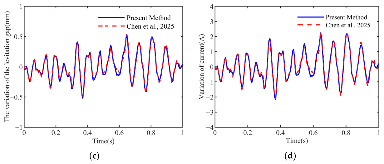
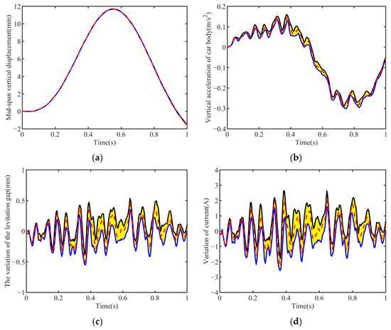
To further clarify the verification procedure, the benchmark results in Ref. [30] were used for comparison, and the results are presented in Figure 3. In the verification process, the vehicle parameters, bridge parameters, boundary conditions, running speed, and track irregularity input were kept the same as those reported in Ref. [30]. The mid-span vertical displacement of the bridge, the vertical acceleration of the car body, the levitation-gap variation, and the current variation were selected as the main comparison quantities.

The blue curve represents the mid-span displacement of the bridge, the vertical acceleration of the car body, the variation of the levitation gap, and the variation of the current calculated by the theoretical model in this paper. The red dotted curve represents the results from the literature [30]. There is a satisfactory agreement between the two, which means the proposed method can obtain various responses of the maglev vehicle–bridge coupled system.

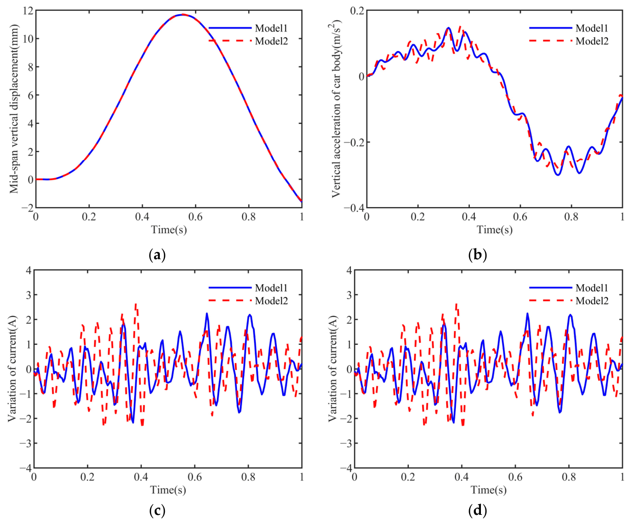
Then, the results of the system responses obtained from two different models are compared, as shown in Figure 4.

It can be concluded that the displacement at the mid-span of the bridge is not affected, the peak value of the car-body acceleration is less affected, while the changes in the levitation gap and current are significantly affected.

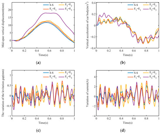
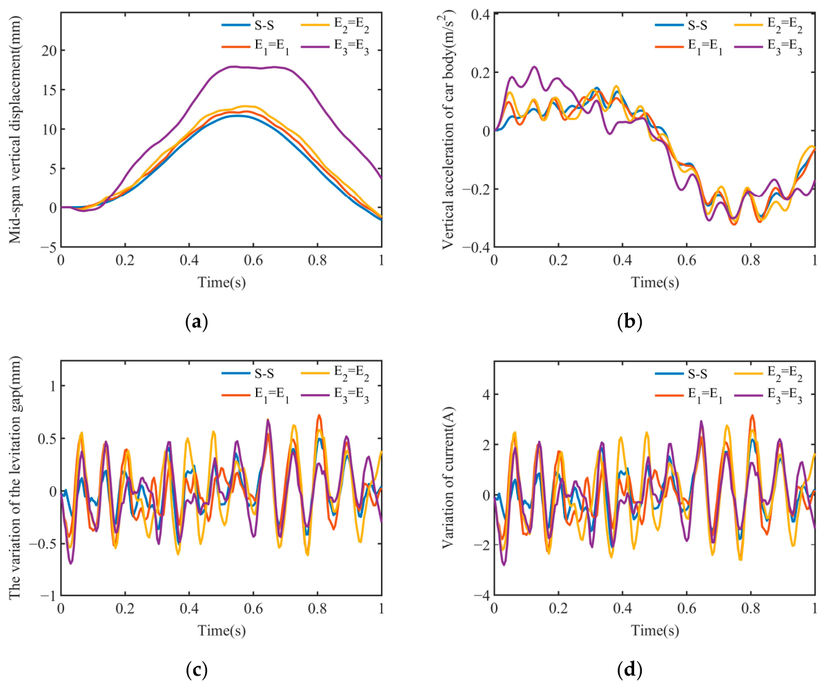
In addition, the effects of typical boundary conditions on the responses of the maglev vehicle–bridge coupled system are shown in Figure 5.

Here, E denotes the elastic restraint, and S denotes the simply supported boundary condition. The stiffness values of the elastic restraints are E₁ = 1 × 10⁷ N/m², E₂ = 5 × 10⁶ N/m², and E₃ = 1 × 10⁶ N/m². The proposed method can effectively simulate different complex boundary conditions. The results indicate that a decrease in the stiffness of the boundary restraints leads to increased vibration responses of both the car body and the guideway beam.

4. Parameter Study

In this paper, to investigate the influence of uncertain suspension parameters and control parameters on the system, the Monte Carlo method is employed for the research. It is necessary to determine the variation range of random parameters. Reference [34] showed that, because of temperature variations, rubber aging, manufacturing errors, and other factors, the variations of suspension parameters may reach up to 100% under actual operating conditions. For most suspension parameters, the variation range caused by parameter errors from −15% to +100% should be considered. In addition, Ref. [35] also indicated that the actual values of suspension parameters may fluctuate between 85% and 115% of their nominal values. It was clearly stated in Ref. [35] that a fluctuation range of ±15% is consistent with the tolerances usually specified for the supply of these railway components. Therefore, this range can be regarded as an acceptable range of parameter dispersion in engineering practice. In the sensitivity analysis presented in this section, to account for the sensitivity characteristics of the vehicle system under extreme operating conditions, the variation range of the suspension parameters was set to 85–200% of the nominal values [34]. The variation range of the control parameters is obtained from the literature [36]. For the three control parameters, the range of the displacement feedback coefficient is 5000 to 10,000, the range of the velocity feedback coefficient is 5 to 20, and the range of the acceleration feedback coefficient is 0.2 to 0.6 [28]. In addition, uniform random sampling was adopted in this study, and the number of samples was set to 100. This sampling scheme allows the parameter space to be explored over the prescribed ranges and can account for the influence of extreme operating conditions.

4.1. Influence of Car-Body Suspension Parameters

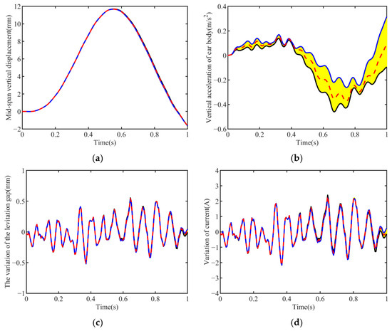
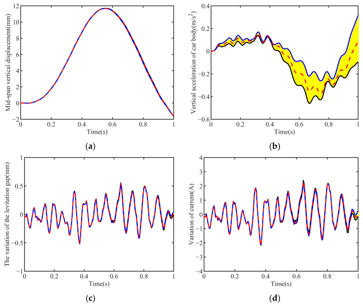
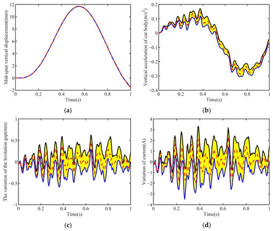
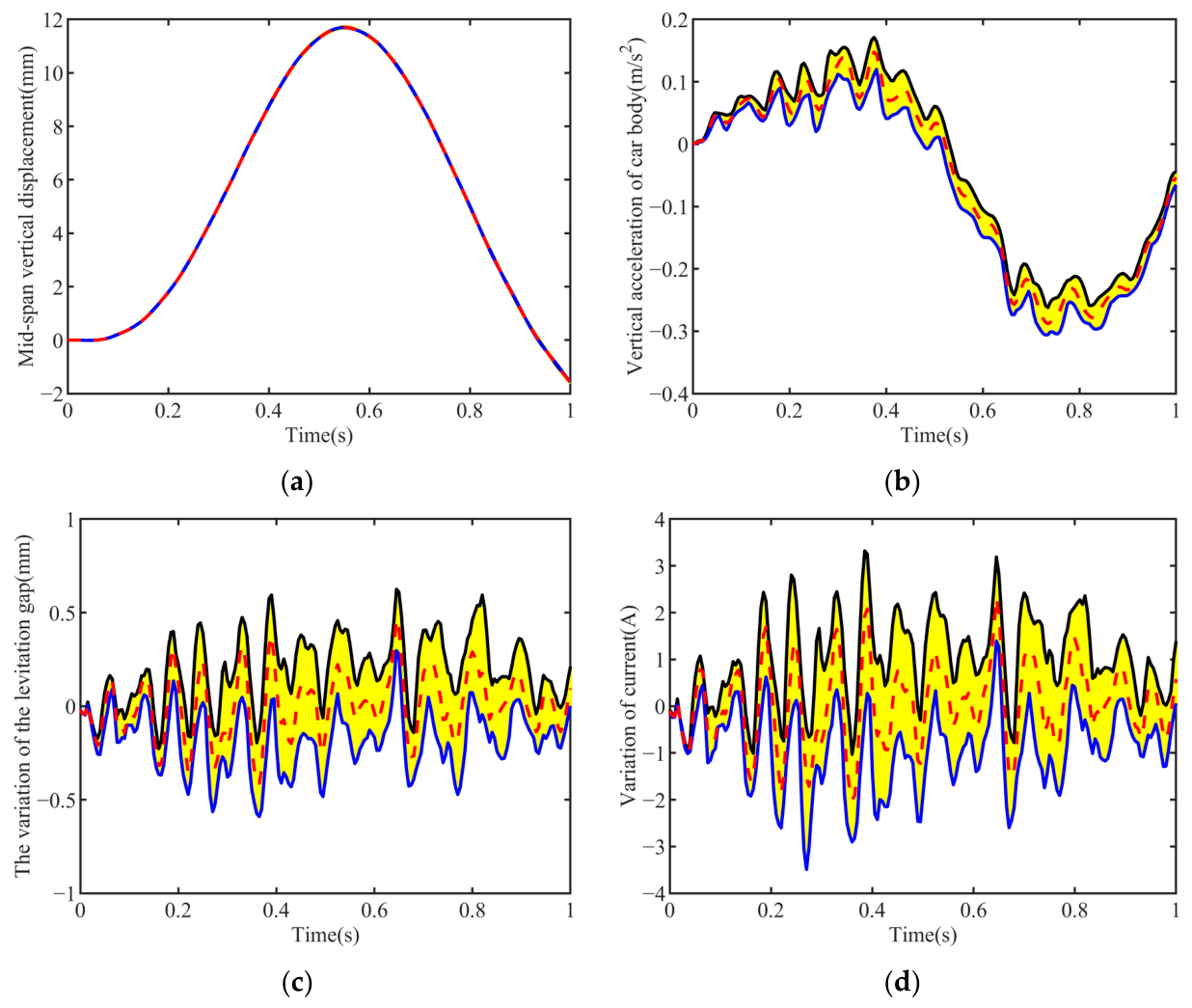
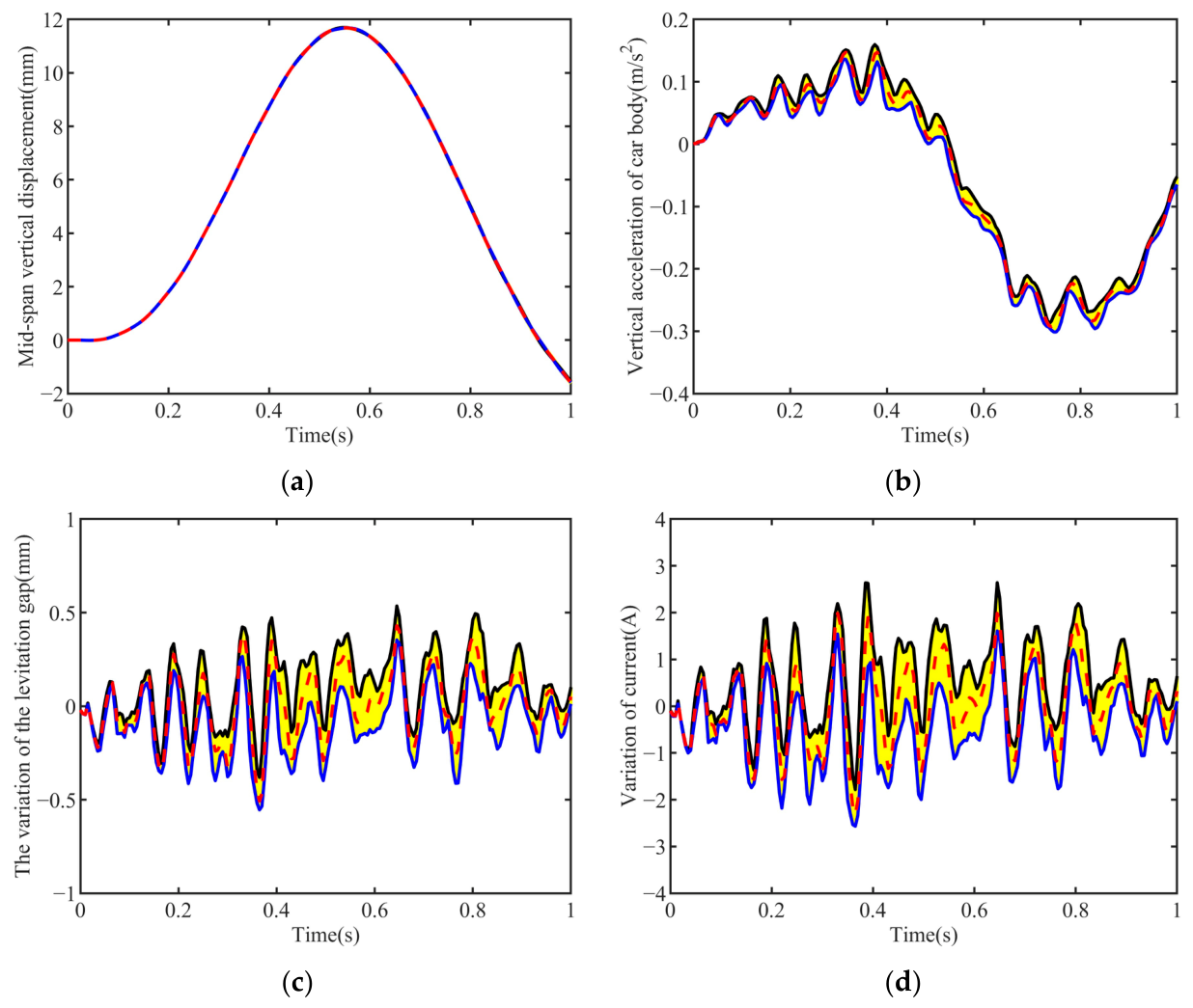
The influences of car-body suspension stiffness on mid-span vertical displacement, car-body vertical acceleration, suspension clearance variation, and current variation can be obtained from Figure 6. Among them, the blue line represents the result of taking the k_s minimum value, the black line represents the result of taking the k_s maximum value, the remaining values are represented by the yellow line, and the red dashed line represents the average value of all results, which is the same in the subsequent images.

With the increase in suspension stiffness, the vertical acceleration of the vehicle body increases as a whole. The mid-span displacement, current variation, and suspension gap variation of the bridge have almost no change. The suspension stiffness of the car body can be reduced appropriately, and the smoothness and comfort of the car body can be improved.

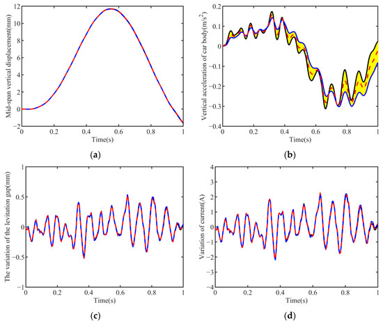
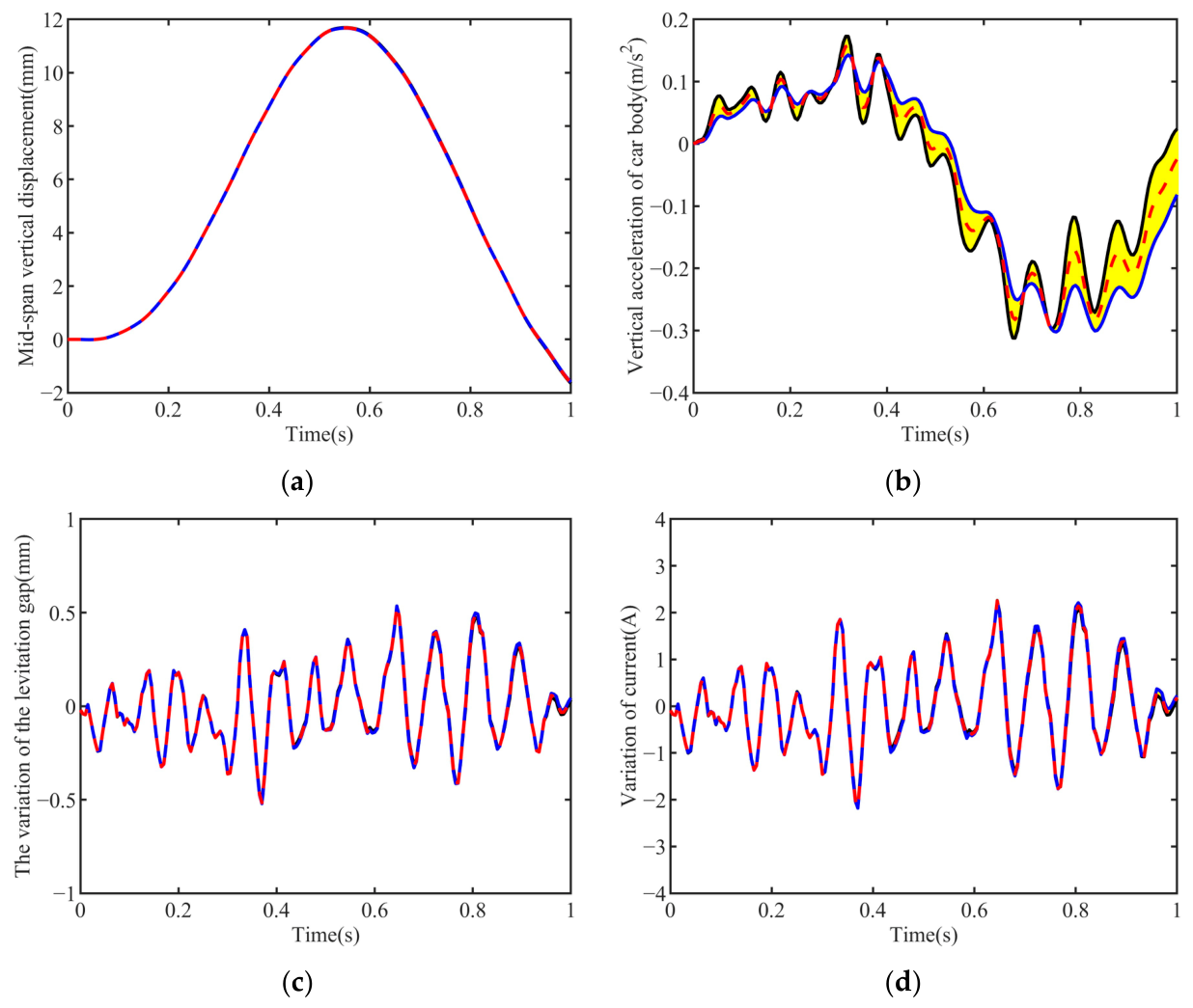
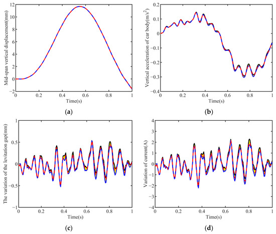
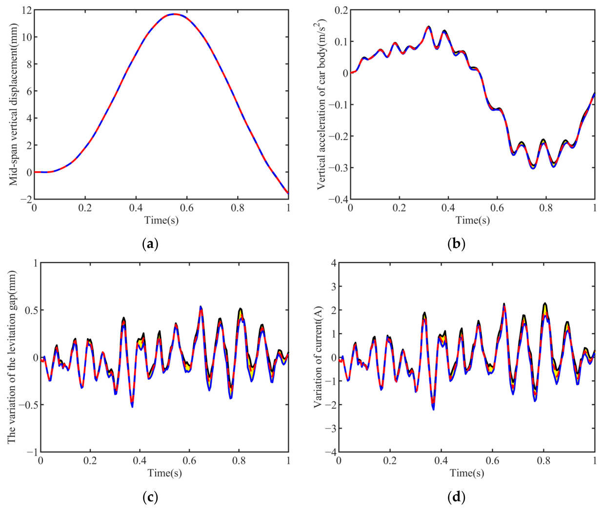
The influences of car-body suspension damping on mid-span vertical displacement, car-body vertical acceleration, suspension clearance variation, and current variation can be obtained from Figure 7.

With the increase of suspension damping, the vertical acceleration oscillation of the vehicle body decreases, but the change is not significant. It mainly affects the time to return to a stable state, and the greater the damping, the faster the recovery speed.

4.2. Influence of Feedback Coefficient

The influences of the displacement feedback coefficient on mid-span vertical displacement, car-body vertical acceleration, suspension clearance variation, and current variation can be obtained from Figure 8.

With the increase of the displacement feedback coefficient, the vertical acceleration of the car body increases gradually. The displacement feedback coefficient G₁ reflects the stiffness effect of the electromagnetic force between the bridge and the electromagnet, and the vertical acceleration of the car-body increases with the increase of the system stiffness.

With the increase of the displacement feedback coefficient, the variation of the electric current increases significantly. The larger the value of the displacement feedback coefficient is, with other parameters remaining constant, the more sensitive the coil current is to the change in the gap. The variation of the current increases to some extent as the value of G₁ increases.

The influences of the velocity feedback coefficient on mid-span vertical displacement, car-body vertical acceleration, suspension clearance variation, and current variation can be obtained from Figure 9.

With the increase of the velocity feedback coefficient, the vertical acceleration of the car body, the variation of current, and the variation of suspension clearance all decrease. The velocity feedback coefficient G₂ reflects the damping effect of the electromagnetic force between the bridge and the electromagnet, which increases the damping of the whole system so that the whole system can stabilize at the rated clearance faster, reduce the vertical acceleration of the car body, and improve the smoothness and comfort of operation.

The influences of the acceleration feedback coefficient on mid-span vertical displacement, car-body vertical acceleration, suspension clearance variation, and current variation can be obtained from Figure 10.

The acceleration feedback coefficient G₃ reflects the mass effect of the electromagnetic force between the bridge and the electromagnet. As the acceleration feedback coefficient increases, the vertical acceleration of the car body is somewhat reduced.

5. Sensitivity Analysis

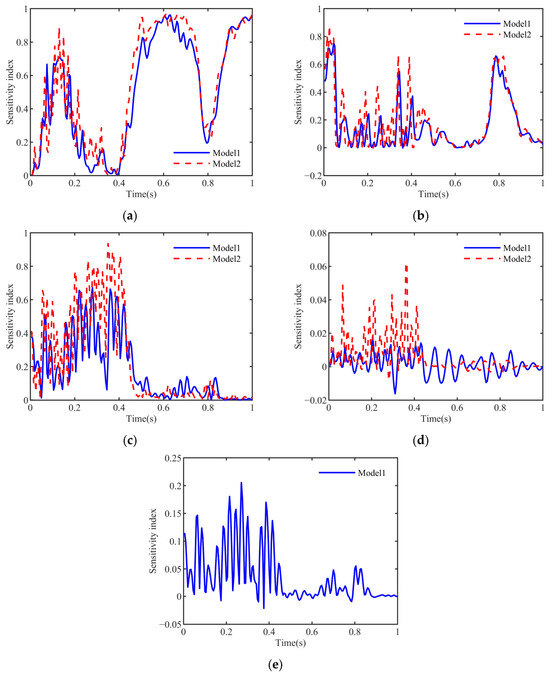
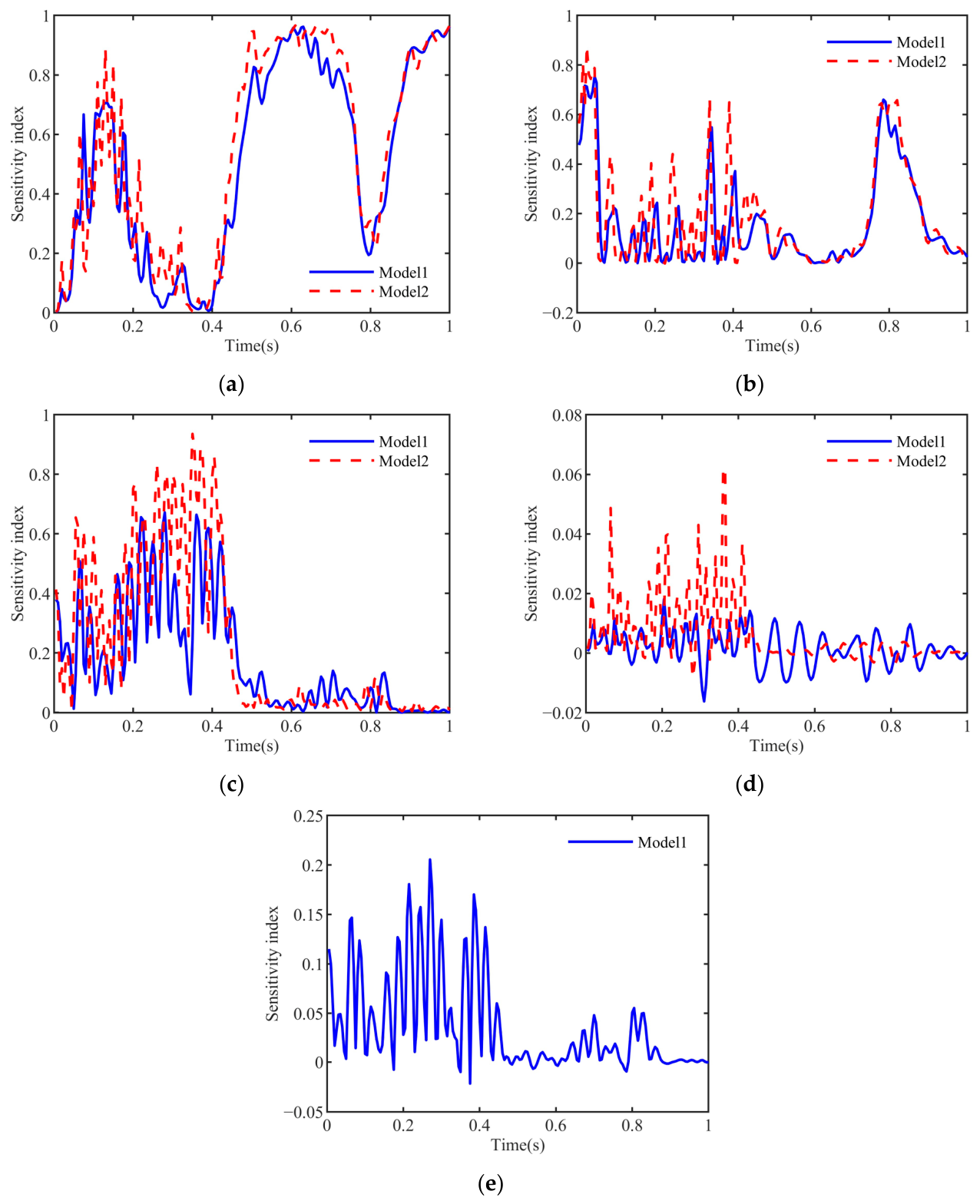
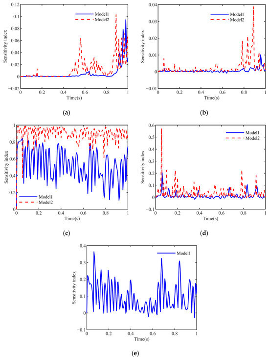
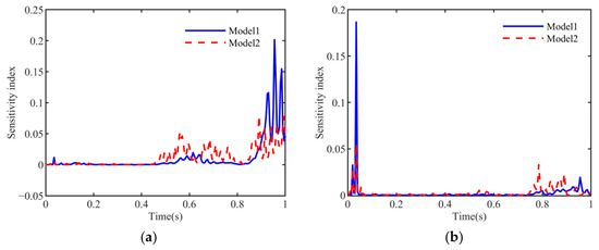
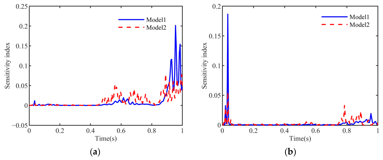
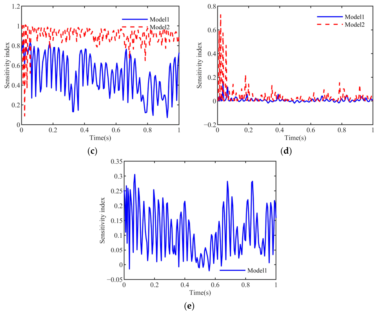
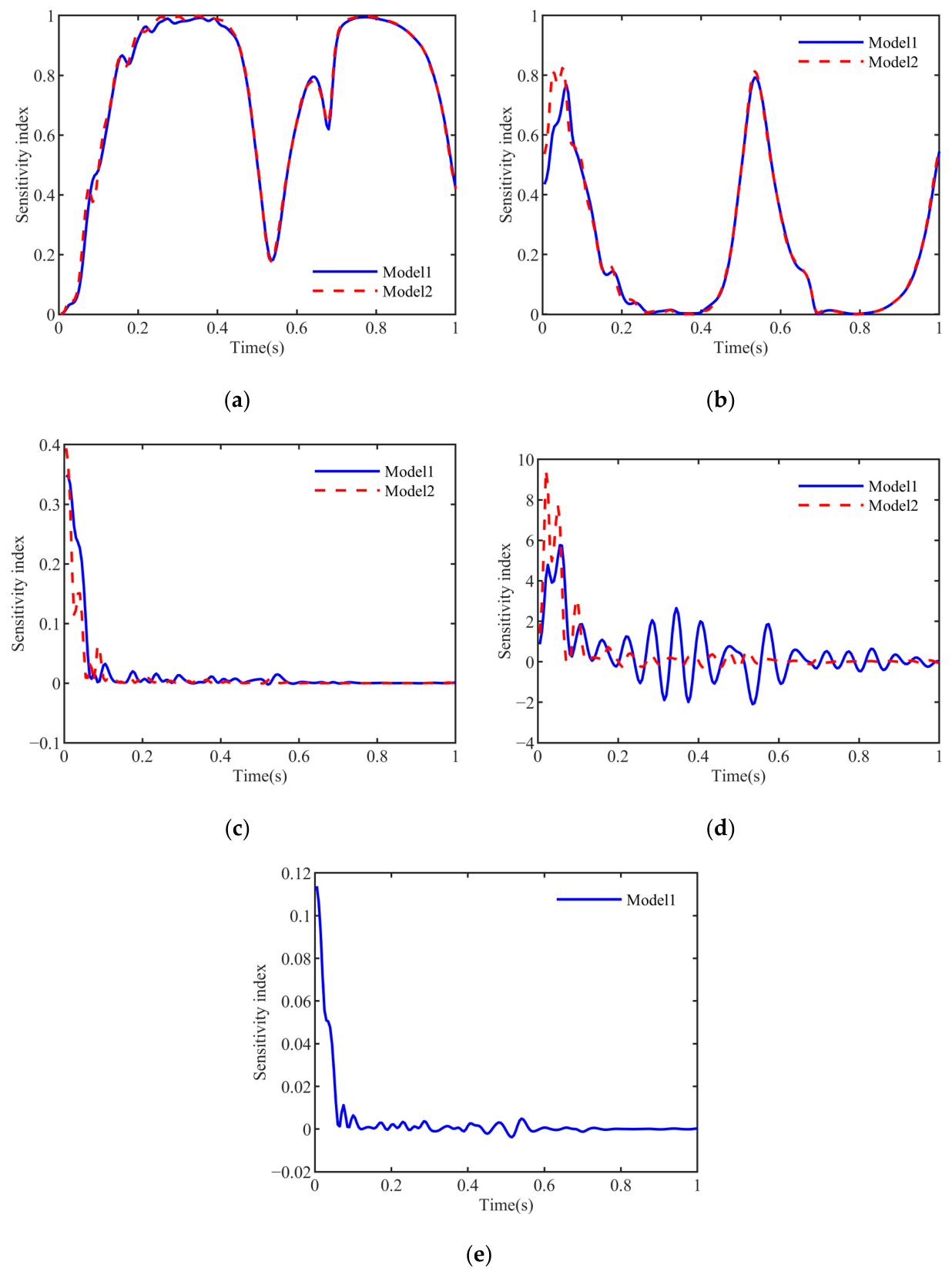
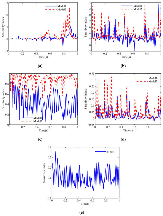
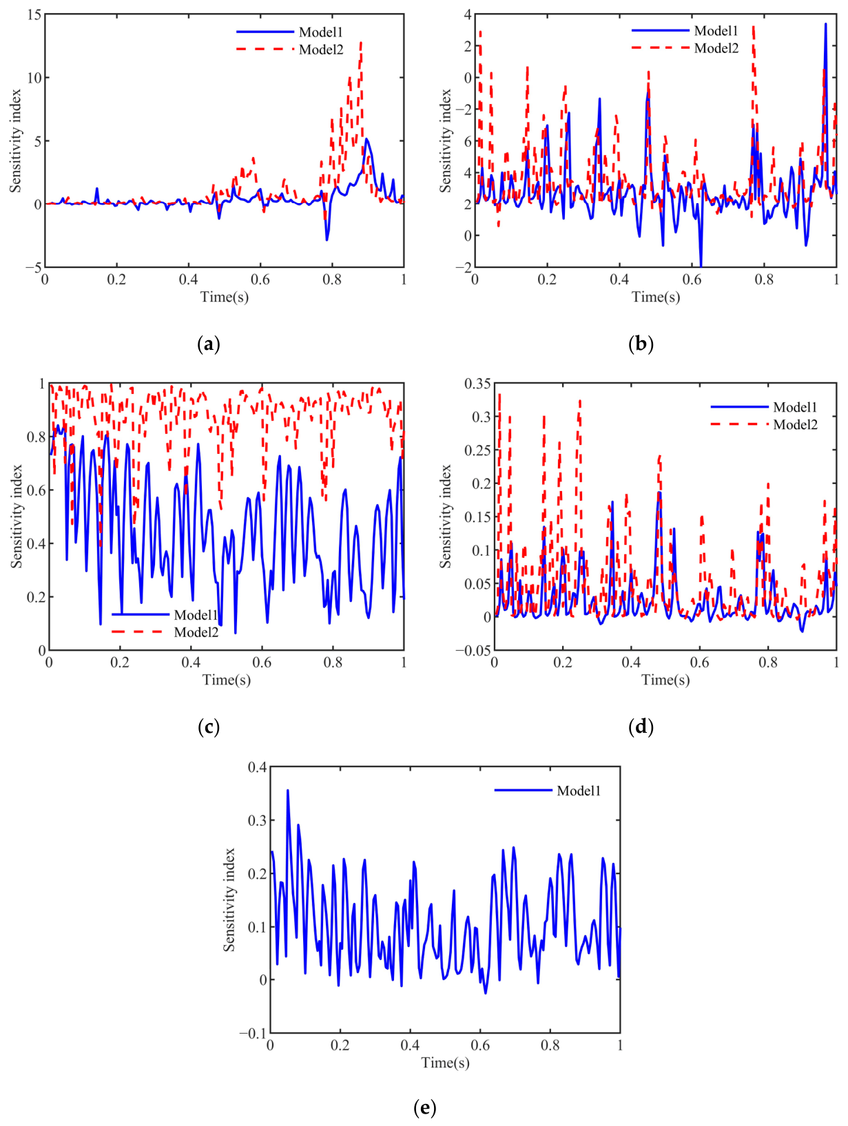
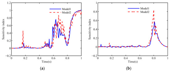
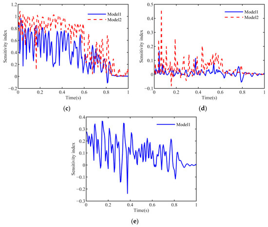
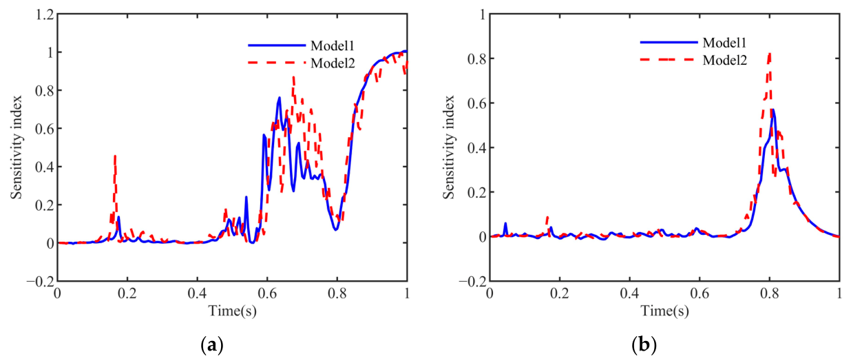
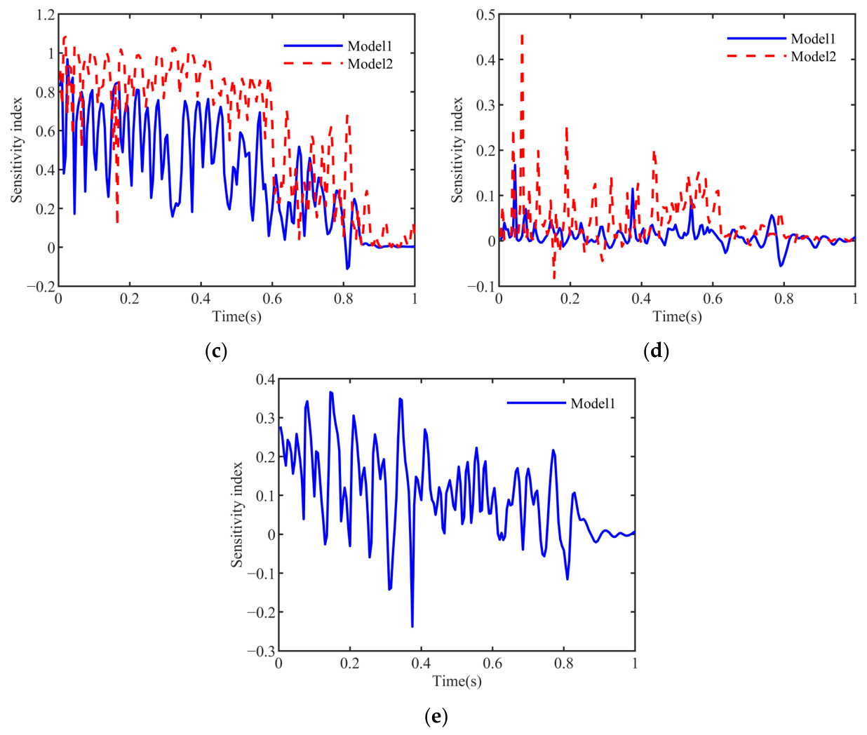
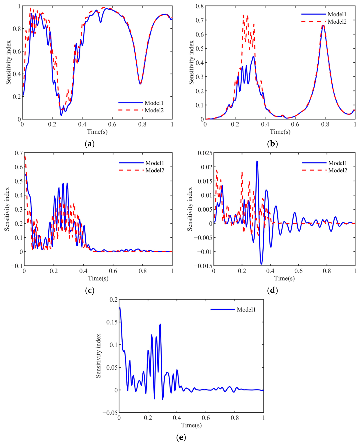
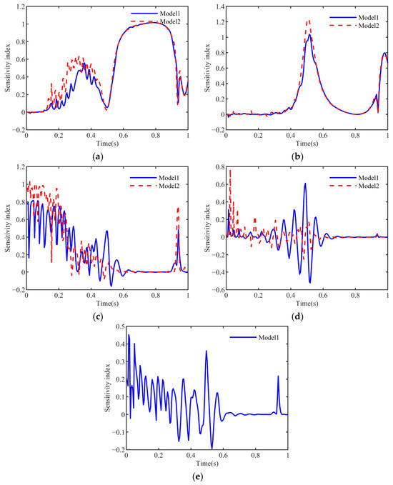
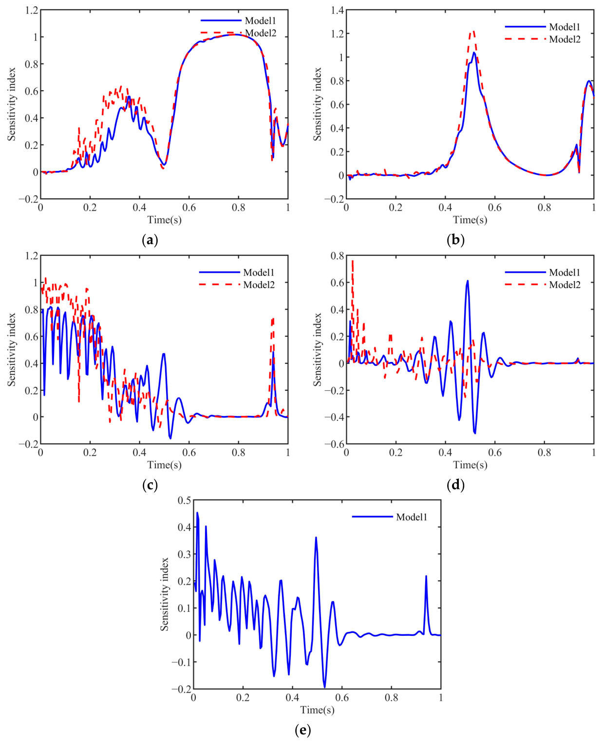
This section analyzes the sensitivity of different responses to the suspension parameters, k_s and c_s, and control parameters G₁, G₂, and G₃. The sensitivity analysis results of Model 1 for the above five parameters are represented by the blue line. The sensitivity analysis results of Model 2 for the four parameters, excluding G₃, are represented by the red dotted line.

5.1. Sensitivity Analysis of the Car-Body Acceleration

The results of the time-history analysis of the sensitivity of the acceleration response of the car body are shown in Figure 11. The mean values and variances of the sensitivity results for each parameter are shown in

Table 3. Mean values and variances of the dimensionless Sobol sensitivity indices for acceleration responses in the two models.

Sensitivity	Method	ks	cs	G1	G2	G3
mean value	Mode1	0.5075	0.1624	0.1799	0.0017	0.0364
variance		0.1118	0.036	0.036	3.33 × 10−5	0.0023
mean value	Mode2	0.5508	0.186	0.2327	0.006
variance		0.1151	0.0453	0.0759	1.22 × 10−4

.

There is little difference in the results of the sensitivity analysis of the car-body acceleration between the two models. The parameter with the highest sensitivity to the acceleration response of the car-body vibration is k_s. The two parameters, c_s and G₁, also exert a certain degree of influence on the acceleration of the car-body vibration. The influences of the other two parameters are relatively negligible.

5.2. Sensitivity Analysis of the Levitation Gap

The results of the sensitivity of the variation of suspension gap are shown in Figure 12. The mean values and variances of the sensitivity results for each parameter are shown in

Table 4. Mean values and variances of the dimensionless Sobol sensitivity indices for the levitation gap in the two models.

Sensitivity	Method	ks	cs	G1	G2	G3
mean value	Mode1	0.005	5.6 × 10−4	0.5329	0.0122	0.0992
variance		1.8 × 10−4	1.5 × 10−6	0.0299	7.18 × 10−4	0.0063
mean value	Mode2	0.011	0.0023	0.90	0.034
variance		2.73 × 10−4	2.1 × 10−5	0.0061	0.0032

.

For the two models, the influences of the two suspension parameters, k_s and c_s, on the suspension gap can be neglected. Among the control parameters, G₁ and G₃ predominantly influence the suspension gap, with G₁ exerting a more significant impact. The sensitivity of G₂ is comparatively low. For the second model, the parameter G₁ exerts an absolute influence, and the average value of its sensitivity reaches 0.9.

5.3. Sensitivity Analysis of the Current

The sensitivity results of the variation of the electric current are shown in Figure 13. The mean values and variances of the sensitivity results for each parameter are shown in

Table 5. Mean values and variances of the dimensionless Sobol sensitivity indices for the current in the two models.

Sensitivity	Method	ks	cs	G1	G2	G3
mean value	Mode1	0.0113	0.0024	0.499	0.0077	0.11
variance		7.94 × 10−4	1.82 × 10−4	0.037	3.72 × 10−4	0.0062
mean value	Mode2	0.0116	0.0023	0.90	0.035
variance		2.6 × 10−4	3.59 × 10−5	0.0107	0.0076

.

The current control includes the variation of the suspension clearance, and the results of the sensitivity analysis are similar. The sensitivities of k_s and c_s, the two suspension parameters, as well as among the control parameters G₂, are all relatively low. Among the control parameters, G₁ and G₃ predominantly influence the variation of electric current, with G₁ exerting a more significant impact. For the second model, the parameter G₁ exerts an absolute influence, and the average value of its sensitivity reaches 0.9.

5.4. Sensitivity Analysis of the Car-Body Kinetic Energy

The sensitivity results of the kinetic energy of the car body are shown in Figure 14. The mean values and variances of the sensitivity results for each parameter are shown in

Table 6. Mean values and variances of the dimensionless Sobol sensitivity indices for the car-body kinetic energy in the two models.

Sensitivity	Method	ks	cs	G1	G2	G3
mean value	Mode1	0.75	0.2	0.018	4.5 × 10−4	0.004
variance		0.08	0.057	0.0036	1.77 × 10−6	2.44 × 10−4
mean value	Mode2	0.76	0.21	0.013	4.73 × 10−4
variance		0.079	0.064	0.0025	2.31 × 10−6

.

The results of the sensitivity analysis of the car-body’s kinetic energy are hardly affected by the two models. The kinetic energy of the car body is mainly affected by k_s and c_s. The values of k_s and c_s can be appropriately adjusted to improve the running smoothness.

5.5. Sensitivity Analysis of the Kinetic Energy of the Levitation Frame

The results of the sensitivity analysis of the kinetic energy of the levitation frame are shown in Figure 15. The mean values and variances of the sensitivity results for each parameter are shown in

Table 7. Mean values and variances of the dimensionless Sobol sensitivity indices for the levitation-frame kinetic energy in the two models.

Sensitivity	Method	ks	cs	G1	G2	G3
mean value	Mode1	4.27 × 10−4	3.79 × 10−4	0.45	0.024	0.1058
variance		8.5 × 10−7	7.89 × 10−7	0.0386	0.0014	0.0057
mean value	Mode2	9.86 × 10−4	7.5 × 10−4	0.88	0.049
variance		3.66 × 10−6	1.14 × 10−6	0.0133	0.0047

.

In both control models, the sensitivities of both k_s and c_s are extremely low. For the three control parameters, in Model 1, G₁ and G₃ mainly affect the kinetic energy of the suspension frame. In Model 2, G₁ and G₂ affect the kinetic energy of the suspension frame. The sensitivity index of G₁ is the highest.

5.6. Sensitivity Analysis of the Vertical Kinetic Energy of the Bridge

The results of the sensitivity analysis of the vertical kinetic energy of the bridge are shown in Figure 16. The mean values and variances of the sensitivity results for each parameter are shown in

Table 8. Mean values and variances of the dimensionless Sobol sensitivity indices for the bridge vertical kinetic energy in the two models.

Sensitivity	Method	ks	cs	G1	G2	G3
mean value	Mode1	0.26	0.05	0.37	0.01	0.099
variance		0.08	0.057	0.0036	1.77 × 10−6	2.44 × 10−4
mean value	Mode2	0.27	0.06	0.60	0.037
variance		0.1166	0.0197	0.1245	0.0033

.

The sensitivity results of the two models are compared, and it is mainly shown that the sensitivity indices of G₁ and G₂ increase. The average value of the sensitivity of G₁ is the highest among both models, and it has a relatively greater influence in the second model. k_s has a relatively significant influence in the second half of the stroke.

5.7. Sensitivity Analysis of the Suspension Potential Energy

The results of the sensitivity analysis of the suspension potential energy are shown in Figure 17. The mean values and variances of the sensitivity results for each parameter are shown in

Table 9. Mean values and variances of the dimensionless Sobol sensitivity indices for the suspension potential energy in the two models.

Sensitivity	Method	ks	cs	G1	G2	G3
mean value	Mode1	0.69	0.15	0.089	9.43 × 10−4	0.0188
variance		0.077	0.026	0.019	2.32 × 10−5	0.0013
mean value	Mode2	0.73	0.18	0.075	0.0018
variance		0.069	0.042	0.015	1.57 × 10−5

.

There is little difference in the results of the sensitivity analysis of the suspension potential energy between the two models. The sensitivity indices of the three control parameters are rather low. The suspension potential energy is significantly influenced by k_s and c_s.

5.8. Sensitivity Analysis of the Potential Energy of the Bridge

The results of the sensitivity analysis of the potential energy of the bridge are shown in Figure 18. The mean values and variances of the sensitivity results for each parameter are shown in

Table 10. Mean values and variances of the dimensionless Sobol sensitivity indices for the bridge potential energy in the two models.

Sensitivity	Method	ks	cs	G1	G2	G3
mean value	Mode1	0.4769	0.1758	0.2204	0.0041	0.0532
variance		0.1489	0.0741	0.0747	0.0189	0.011
mean value	Mode2	0.5207	0.1935	0.2549	0.016
variance		0.1365	0.0962	0.1196	0.0075

.

The results of the sensitivity analysis are compared. After eliminating the parameter G₃, the sensitivity of the parameter G₁ increases, while the sensitivities of other parameters change slightly. The potential energy of the bridge is mainly influenced by k_s and G₁.

6. Discussion

(1)

When the stiffness of the car-body suspension increases, the overall vertical acceleration of the car body also increases. It is advisable to appropriately reduce the stiffness of the vehicle body suspension, thereby enhancing the running stability and comfort.

(2)

The damping of the car-body suspension mainly affects the time required to return to the stable state. The greater the suspension damping, the faster the return speed.

(3)

The vertical acceleration of the car body increases with the increase of the displacement feedback coefficient. The displacement feedback coefficient should not be too small, which may lead to the instability of the levitation, nor should it be too large, which will significantly increase the dynamic response of the system.

(4)

The velocity feedback coefficient can be appropriately increased to enhance the stability of the system.

(5)

The acceleration feedback coefficient G₃ reflects the mass effect of the electromagnetic force between the bridge and the electromagnet.

(6)

The sensitivity analysis results of the two models are compared. The changes in k_s and c_s are relatively small, and mainly G₁ and G₂ are affected.

References

- Li, F.; Sun, Y.; Xu, J.; He, Z.; Lin, G. Control methods for levitation system of EMS-type maglev vehicles: An overview. Energies 2023, 16, 2995. [Google Scholar] [CrossRef] [Scilit]
- Jian, D.; Yi, G.J.L.; Keng, K.A. Dynamic Response Analysis of High-Speed Maglev-Guideway System. J. Vib. Eng. Technol. 2023, 11, 2647–2658. [Google Scholar]
- Wang, S.; Ni, Y.; Sun, Y.; Lu, Y.; Duan, Y. Modelling dynamic interaction of maglev train–controller–rail–bridge system by vector mechanics. J. Sound Vib. 2022, 533, 117023. [Google Scholar]
- Mao, J.; Wang, X.; Li, Z.; Li, D.; Khan, M.; Yu, Z. A PDEM-Driven Method for Stochastic Parameter Analysis and Running Safety Reliability Assessment in High-Speed Maglev Train-Bridge Coupled System. Int. J. Struct. Stab. Dyn. 2025, 2650391. [Google Scholar] [CrossRef] [Scilit]
- Mao, J.; Li, D.; Yu, Z.; Cai, W.; Guo, W.; Zhang, G. A novel refined dynamic model of high-speed maglev train-bridge coupled system for random vibration and running safety assessment. J. Cent. South Univ. 2024, 31, 2532–2544. [Google Scholar]
- Huang, F.; Cheng, B.; Trng, N. A numerical model to predict three-dimensional interaction dynamic of low-medium-speed maglev vehicle–guideway bridge system. Proc. Inst. Mech. Eng. Part F J. Rail Rapid Transit 2021, 235, 1249–1267. [Google Scholar]
- Huang, F.; Wang, J.; Teng, N.; Cheng, B. Coupled vibration of low-medium-speed maglev vehicle-guideway system on isolated bridge with lead rubber bearings. Adv. Struct. Eng. 2024, 27, 2391–2408. [Google Scholar]
- Liu, W.; Guo, W. Random vibration analysis of coupled three-dimensional maglev vehicle-bridge system. Adv. Civ. Eng. 2019, 2019, 4920659. [Google Scholar]
- Song, Y.; Lin, G.; Ni, F.; Xu, J.; Chen, C. Study on coupled vertical vehicle-bridge dynamic performance of medium and low-speed maglev train. Appl. Sci. 2021, 11, 5898. [Google Scholar]
- Wang, H.; Deng, Z.; Ma, S.; Sun, R.; Li, H.; Li, J. Dynamic Simulation of the HTS maglev vehicle-bridge coupled system based on levitation force experiment. IEEE Trans. Appl. Supercond. 2019, 29, 3601606. [Google Scholar] [CrossRef] [Scilit]
- Deng, Z.; Li, J.; Wang, H.; Li, Y.; Zheng, J. Dynamic simulation of the vehicle/bridge coupled system in high-temperature superconducting maglev. Comput. Sci. Eng. 2019, 21, 60–71. [Google Scholar]
- Hu, J.; Ma, W.; Luo, S. Coupled dynamic analysis of low and medium speed maglev vehicle-bridge interaction using SIMPACK. Proc. Inst. Mech. Eng. Part F J. Rail Rapid Transit 2021, 235, 377–389. [Google Scholar]
- Zhang, P.; Yu, Z. Stochastic dynamic analysis for a three-dimensional maglev vehicle-guideway interaction system based on probability density evolution method considering uncertain parameters. Structures 2025, 73, 108371. [Google Scholar]
- Wang, L.; Bu, X.; Hu, P.; Han, Y.; Cai, C. Dynamic reliability analysis of running safety and stability of a high-speed maglev train on a guideway bridge. Int. J. Struct. Stab. Dyn. 2024, 24, 2450043. [Google Scholar]
- Feng, Y.; Zhao, C.; Wu, D.; Xie, H.; Tong, L. Effect of levitation gap feedback time delay on the EMS maglev vehicle system dynamic response. Nonlinear Dyn. 2023, 111, 7137–7156. [Google Scholar] [CrossRef] [Scilit]
- Liu, W.; Guo, W. Vibration analysis of EMS-type maglev vehicles traveling over a long-span bridge with double lines. KSCE J. Civ. Eng. 2020, 24, 1531–1544. [Google Scholar]
- Liang, X.; Jiang, T.; Hong, Y.; Zhang, J.; Jiang, M.; Wang, Z. Vibration response analysis of simply supported box girder bridge-maglev train in accelerated test of Changsha maglev express. Adv. Mater. Sci. Eng. 2020, 2020, 9563747. [Google Scholar]
- Li, Y.; Tian, X.; Xiang, H.; Zhu, J. Dynamic analysis of a coupled system of high-speed maglev train and a flexible long-span continuous rigid frame bridge. Int. J. Struct. Stab. Dyn. 2023, 23, 2350174. [Google Scholar]
- Zhang, M.; Yuan, C.; Ma, W.; Luo, S. Effect of suspension form on the vehicle-bridge coupled vibration of the maglev vehicle. Veh. Syst. Dyn. 2024, 62, 511–532. [Google Scholar]
- Xu, C.; Luo, H.; Gan, X.; Liu, M.; Guo, H. Research on coupled vibrations between the low-to-medium speed maglev train and a long-span continuous beam bridge. Structures 2023, 56, 104927. [Google Scholar]
- Chen, C.; Xu, J.; Lu, Y.; Lin, G.; Ji, W. Experimental study on vertical vehicle-rail-bridge coupling of medium and low speed maglev train based on track beam with different stiffness. J. Vib. Control 2023, 29, 4129–4142. [Google Scholar]
- Xia, W.; Zeng, J.; Dou, F.; Long, Z. Method of combining theoretical calculation with numerical simulation for analyzing effects of parameters on the maglev vehicle-bridge system. IEEE Trans. Veh. Technol. 2021, 70, 2250–2257. [Google Scholar] [CrossRef] [Scilit]
- Wen, L.; Zhou, K.; Yang, T.; Fu, S.; Gong, D.; Zhou, J. Energy based formulation for dynamic modelling and random vibration analysis of high-speed vehicle system. Eur. J. Mech. A/Solids 2026, 115, 105828. [Google Scholar]
- Sun, Y.; He, Z.; Xu, J.; Sun, W.; Lin, G. Dynamic analysis and vibration control for a maglev vehicle-guideway coupling system with experimental verification. Mech. Syst. Signal Process. 2023, 188, 109954. [Google Scholar]
- Sun, Y.; Xu, J.; Qiang, H.; Wang, W.; Lin, G. Hopf bifurcation analysis of maglev vehicle–guideway interaction vibration system and stability control based on fuzzy adaptive theory. Comput. Ind. 2019, 108, 197–209. [Google Scholar] [CrossRef] [Scilit]
- Talukdar, R.P.; Talukdar, S. Dynamic analysis of high-speed maglev vehicle–guideway system: An approach in block diagram environment. Urban Rail Transit 2016, 2, 71–84. [Google Scholar]
- Yang, Y.; Liu, C.; Chen, L.; Zhang, X. Phase deviation of semi-active suspension control and its compensation with inertial suspension. Acta Mech. Sin. 2024, 40, 523367. [Google Scholar] [CrossRef] [Scilit]
- Wen, L.; Yang, T.; Zhou, K.; Li, C.; Zhang, Z.; Gong, D.; Zhou, J. Efficient three-dimensional dynamic model and coupled vibration analysis of vehicle system with underframe suspended equipment. Eur. J. Mech. A/Solids 2026, 119, 106182. [Google Scholar] [CrossRef] [Scilit]
- Zhou, K.; You, T.; Gong, D.; Zhou, J. Effects of uncertain suspension parameters on dynamic responses of the railway vehicle system. Probabilistic Eng. Mech. 2023, 71, 103405. [Google Scholar]
- Chen, R.; Lu, Z.R.; Su, C.; Ni, Y. Stochastic optimization of levitation control system for maglev vehicles subjected to random guideway irregularity. J. Sound Vib. 2025, 594, 118682. [Google Scholar]
- Zhou, F.; Li, X. Coupled dynamics modeling and validation of maglev vehicle and bridge systems. Actuators 2025, 14, 107. [Google Scholar] [CrossRef] [Scilit]
- Wang, B.; Zhang, Y.; Xia, C.; Li, Y.; Gong, J. Dynamic analysis of high-speed maglev train-bridge system with fuzzy proportional-integral-derivative control. J. Low Freq. Noise Vib. Act. Control 2022, 41, 374–386. [Google Scholar]
- Zhao, C.F.; Zhai, W.M. Maglev vehicle/guideway vertical random response and ride quality. Veh. Syst. Dyn. 2002, 38, 185–210. [Google Scholar] [CrossRef] [Scilit]
- Wang, Y. Dynamics and Load Analysis of High-Speed Trains Considering Stochastic Factors. Master’s Thesis, Southwest Jiaotong University, Chengdu, China, 2018. [Google Scholar]
- Mazzola, L.; Bruni, S. Effect of suspension parameter uncertainty on the dynamic behaviour of railway vehicles. Appl. Mech. Mater. 2011, 104, 177–185. [Google Scholar]
- Wen, L.; Zhou, K.; Gong, D.; Zhou, J. Research on the stochastic vertical vibration characteristics of the coupled high-speed train vehicle system. J. Vib. Control 2025, 32, 256–268. [Google Scholar] [CrossRef] [Scilit]
Disclaimer/Publisher’s Note: The statements, opinions and data contained in all publications are solely those of the individual author(s) and contributor(s) and not of MDPI and/or the editor(s). MDPI and/or the editor(s) disclaim responsibility for any injury to people or property resulting from any ideas, methods, instructions or products referred to in the content. |
© 2026 by the authors. Licensee MDPI, Basel, Switzerland. This article is an open access article distributed under the terms and conditions of the Creative Commons Attribution (CC BY) license.