Data-Driven Defect Prediction for Manufacturing Quality Monitoring Under Class Imbalance and Missing Data: A Performance–Efficiency Trade-Off Analysis

Abstract

Manufacturing equipment logs are an important source of information for quality monitoring, but building reliable defect prediction models from such logs is still difficult in practice. Defective samples are rare, and many process variables are missing because measurements are recorded only under certain sensing or process conditions. These properties make defect prediction difficult and limit the usefulness of accuracy-based evaluation. This paper evaluates defect prediction using the Bosch Production Line Performance dataset, with a supplementary validation experiment on the semiconductor manufacturing process (SECOM) dataset. Two feature configurations are compared: a baseline representation using imputed numerical variables and a missingness-aware representation that adds feature-wise missing indicators and a sample-level missing ratio. Logistic Regression, Random Forest, and LightGBM are evaluated using validation-based threshold selection. To examine the effect of imputation choice, zero, median, and KNN imputation are also compared in the SECOM experiment. In the Bosch experiment, explicitly representing missingness improves PR-AUC for all tested model configurations. The supplementary SECOM experiment shows a more mixed pattern, suggesting that the usefulness of missingness-aware features depends on the dataset, imputation strategy, and model family. The latency analysis further shows a practical trade-off: Random Forest with missingness-aware features gives the highest PR-AUC on Bosch but has the highest inference latency, while LightGBM provides a more balanced choice when prediction performance and response time are considered together.

1. Introduction

Modern production lines continuously generate equipment log data during routine operation. Although these logs are originally collected for monitoring, traceability, and process control, they also contain useful clues about abnormal operating conditions. In this sense, defect prediction from equipment logs is a practical way to support early quality intervention before defective products move further downstream [1,2].

Applying supervised learning to this type of log data is not straightforward. The first issue appears in the class distribution. In a stable production line, defective products are expected to be rare, so the number of positive samples is much smaller than the number of normal samples. A classifier trained on such data can achieve high overall accuracy while still missing most of the defective cases. For this reason, accuracy alone is not a reliable measure of defect-prediction performance under rare-event conditions [3,4,5]. In quality monitoring, the minority class is usually the class of interest, because missed defects can lead to additional inspection cost, rework, scrap, or process instability [2].

Missing values are another practical issue in equipment-log data. In many production datasets, not every variable is recorded for every product or process stage. Missing values may arise from sensor faults, communication delays, stage-dependent measurement policies, or inspection routines that are triggered only under certain conditions. These missing values are often handled through deletion or simple imputation. However, in manufacturing data, missingness itself may carry information about process state, sensor availability, or equipment behavior [6,7,8,9]. Treating all missing values only as noise may therefore remove useful signals from the data.

The final issue considered in this paper is whether the model can be used within a realistic production cycle. Even when a classifier gives good prediction scores, it is difficult to deploy if the inference time is too long for near-real-time monitoring. Conversely, a simpler model with slightly weaker discrimination may be preferable when response time is critical. Recent studies in manufacturing analytics have therefore emphasized the need to evaluate predictive models together with their operational constraints [10,11].

This paper examines these issues using the Bosch Production Line Performance dataset, a large manufacturing log dataset that contains both rare defects and many missing numerical entries [12]. The focus is not on introducing another classifier, but on checking how standard models behave when the data representation and deployment constraints are changed. Specifically, the study compares a zero-imputed feature set with a missingness-aware feature set, evaluates the models using PR-AUC and validation-selected high-precision thresholds, and measures p95 inference latency for Logistic Regression, Random Forest, and LightGBM.

The main contributions of our study are as follows: First, it provides a controlled empirical evaluation of defect prediction models under severe class imbalance in smart manufacturing log data, focusing on Logistic Regression, Random Forest, and LightGBM under a fixed and reproducible data partition. Second, it systematically investigates the effect of missingness-aware feature representation by comparing standard imputed features with explicit missing indicators and a sample-level missing ratio, demonstrating how missing data can be exploited as informative signals rather than treated solely as noise. Third, it analyzes the trade-off between predictive performance and operational efficiency by jointly considering PR-AUC, validation-based high-precision thresholding, and p95 inference latency and further evaluates the generalizability of findings through supplementary experiments on an external semiconductor manufacturing process (SECOM) dataset.

2. Related Work

2.1. Defect Prediction and Data-Driven Quality Monitoring in Manufacturing

Machine learning has been widely used in manufacturing for predictive maintenance, process monitoring, and quality-related decision support. In these applications, process measurements and equipment logs can provide early evidence of abnormal behavior before a quality failure is observed [1]. Recent reviews also show that data-driven quality monitoring is becoming a central part of smart manufacturing, particularly when complex process interactions make rule-based inspection difficult [10,11].

Defect prediction from manufacturing logs differs from many standard tabular classification tasks. The data are usually high-dimensional, process-dependent, and collected under operating conditions that were not designed specifically for machine learning. Related studies have applied AI-based inspection and quality evaluation to manufacturing problems such as machine-vision defect detection and surface-quality assessment [13,14]. These studies show the usefulness of machine learning in manufacturing, but they also highlight the need to consider the characteristics of the production data and the requirements of deployment.

2.2. Class Imbalance in Manufacturing Data

Class imbalance is a typical characteristic of manufacturing defect data. Since production systems are designed to reduce failures, defective samples are usually much fewer than normal samples. This imbalance is not simply a sampling problem; it reflects the actual operating condition of the production line [2]. A model trained on such data may focus on the majority class and still appear to perform well when evaluated using aggregate metrics.

Common approaches to imbalanced learning include resampling, cost-sensitive learning, and model-level class weighting [3]. In manufacturing, however, aggressive over-sampling or under-sampling can be problematic because it changes the empirical distribution of process states. For this reason, this study uses model-level imbalance handling while preserving the original data distribution. This choice is intended to keep the experimental setting closer to the observed production data.

2.3. Evaluation Under Rare Defect Conditions

When the positive class is rare, the choice of evaluation metric has a strong effect on the interpretation of model performance. Accuracy can be misleading because most observations belong to the non-defect class. ROC-AUC can also look optimistic when negative samples dominate the dataset. Precision–recall analysis is often more informative in this setting because it focuses directly on the relationship between detected defects and false alarms [4,5].

For manufacturing quality monitoring, this relationship is operationally important. A high false-alarm rate can increase unnecessary inspection and reduce operator trust, whereas low recall means that defective products may pass through the monitoring system. Evaluation should therefore include both threshold-independent ranking performance and behavior at an operating point. In this study, PR-AUC is used together with test recall at validation-selected high-precision thresholds to reflect both aspects of model performance [15].

2.4. Missing Information in Manufacturing Logs

Missing values are common in manufacturing logs. They may occur because a sensor fails to report, a measurement is available only at a particular process stage, or an inspection step is not performed for every product. Although missing-data methods are often discussed as a preprocessing problem, the pattern of missingness can also affect prediction performance [6].

Recent manufacturing studies have proposed imputation methods for recovering missing process values, especially in monitoring and soft-sensor applications [7,9]. These methods are useful when the goal is to estimate plausible numerical values. In defect prediction, however, the fact that a value is missing may also be informative. The missing indicator method provides a simple way to retain this information by adding binary variables that mark missing entries [8]. Its effect has not been studied extensively in combination with severe class imbalance and deployment-oriented evaluation in manufacturing defect prediction.

2.5. Spatial-Temporal and Adaptive Modeling in Industrial Processes

Recent industrial quality prediction studies have increasingly considered spatial and temporal dependencies among process variables [16]. For example, GraphSiamese has been proposed as a spatial-temporal slow feature fusion network for industrial process quality prediction, using graph-based structures to represent relationships among process variables and temporal slow dynamics. Such approaches are useful when the physical or temporal relationships among variables are available or can be inferred from process data.

Another related direction is adaptive modeling under changing operating conditions. In practical manufacturing environments, sensor degradation, maintenance events, product-mix changes, and seasonal effects can change the data distribution over time. Recent work on self-modified dynamic domain adaptation for industrial soft sensing addresses this issue by considering both distribution discrepancy and dynamic feature transfer [17]. These studies highlight an important limitation of static train-validation-test evaluation. The present study focuses on lightweight tabular models and missingness-aware feature construction, but the effect of spatial-temporal structure and domain shift remains an important direction for future work.

2.6. Research Gap and Positioning of This Study

Previous studies provide useful foundations for defect prediction, imbalanced learning, missing-data handling, and industrial quality prediction. However, these issues are often treated separately. Many manufacturing defect prediction studies still emphasize aggregate predictive performance, while the behavior of models under rare-defect operating conditions receives less attention. Missing values are also commonly handled as a preprocessing issue, although their occurrence may be related to process states, sensing availability, or inspection logic. In addition, spatial-temporal modeling and domain-adaptive learning have recently advanced in industrial quality prediction and soft sensing, but these approaches are usually studied separately from lightweight deployment-oriented defect prediction.

This study addresses these points through an empirical evaluation of defect prediction models on manufacturing log data. The proposed comparison combines PR-AUC and validation-selected threshold evaluation for class imbalance, explicit missingness representation through missing indicators and a missing ratio, p95 latency measurement for operational feasibility, and supplementary validation on an additional SECOM dataset. This framing positions the work as a deployment-oriented analysis rather than a purely accuracy-driven benchmark.

3. Methodology

The experimental procedure was organized to keep the comparison between feature sets and models as consistent as possible. The main experiment used the sampled Bosch dataset, and an additional experiment used the SECOM dataset to check whether the main observations were specific to a single manufacturing dataset. The main elements were the two feature representations, the three classification models, the imbalance-handling settings, the validation-based threshold protocol, and the latency measurement procedure.

3.1. Dataset and Feature Construction

The experiments used the numerical part of the Bosch Production Line Performance dataset, which contains manufacturing process measurements collected across multiple production stages [12]. We used a stratified random sample of 300,000 observations so that the experiment remained computationally manageable while keeping the rare-defect ratio close to the original data. After removing the identifier column, the dataset contained 968 numerical variables. Among the sampled observations, 1743 were defective, corresponding to a positive-class ratio of 0.5810%. This level of imbalance is consistent with practical quality-monitoring settings, where defective products are much less frequent than normal production instances [2,3].

To examine whether the Bosch-based findings were specific to a single dataset, a supplementary experiment was conducted using the SECOM dataset [18]. The SECOM dataset contains measurements from a semiconductor manufacturing process and includes missing values and imbalanced pass/fail labels. After removing the time column and constant or single-value features, the dataset contained 1567 observations and 474 process variables. The target variable was the pass/fail label, with 104 defective observations, corresponding to a positive-class ratio of 6.64%. The raw missing-value rate after preprocessing was 5.54%. The same missingness-aware feature construction was applied to SECOM, resulting in 474 missing indicators and 949 variables in Feature Set B.

Two feature configurations were prepared to examine whether missingness carries useful information for defect prediction. Feature Set A used the imputed numerical variables only. For Bosch, this resulted in 968 variables and zero imputation was used in the main experiment. For SECOM, this resulted in 474 variables after preprocessing, and Feature Set A was constructed separately under zero, median, and KNN imputation baselines. This setting gives a basic reference case: the numerical matrix is completed, but the information about which entries were originally missing is discarded.

Feature Set B extended Feature Set A by adding explicit missingness information. For each original numerical variable, a binary indicator was created to record whether the value was originally missing. In addition, a sample-level missing ratio was computed to represent the proportion of unavailable measurements in each observation. For Bosch, Feature Set B contained 1937 variables: 968 zero-imputed numerical variables, 968 missing indicators, and one missing-ratio feature. For SECOM, Feature Set B contained 949 variables: 474 imputed process variables, 474 missing indicators, and one missing-ratio feature.

The reason for adding these variables is that missing values in manufacturing logs are not necessarily random. For example, a value may be missing because a certain measurement is not taken at a specific process stage, because a sensor is inactive under a given operating condition, or because an inspection step is skipped. If this is the case, the missingness pattern can describe part of the production process. Comparing Feature Sets A and B therefore tests whether such information is useful beyond zero imputation alone [6,7,8,9].

3.2. Classification Models and Imbalance Handling

The comparison used three classifiers with different levels of complexity: Logistic Regression (LR), Random Forest (RF), and LightGBM (LGBM). Logistic Regression was included as a fast linear baseline. Random Forest was used to represent a bagging-based tree ensemble that can model nonlinear relations and feature interactions [19]. LightGBM was selected as the gradient-boosting model because it is designed for efficient learning on large-scale structured data [20]. Although XGBoost also belongs to the same broader family of scalable tree-boosting methods [21], it was not included in the experimental comparison.

Each model was tested in a default setting and in an imbalance-aware setting. For Logistic Regression and Random Forest, the imbalance-aware configuration employed balanced class weights (i.e., class_weight=‘balanced’), which assign weights inversely proportional to the frequency of each class. For LightGBM, the corresponding option was is_unbalance=True. These settings were used because they modify the training loss or class weighting without resampling the data. This was important for the present dataset, since over-sampling or under-sampling could change the observed distribution of process states in the manufacturing logs [2,3].

The main hyperparameters were fixed before evaluation. This was done to focus the comparison on the effects of feature representation, model family, and imbalance handling rather than on extensive dataset-specific tuning. The model-specific hyperparameter settings are summarized in Table 1. Other parameters were left at their library defaults unless otherwise specified.

Table 1. Model-specific hyperparameter configuration.

Model	Parameter	Value
Logistic Regression	solver	lbfgs
Logistic Regression	max_iter	1000
Logistic Regression	class_weight	None/balanced
Random Forest	n_estimators	200
Random Forest	random_state	42
Random Forest	class_weight	None/balanced
LightGBM	n_estimators	800
LightGBM	learning_rate	0.05
LightGBM	num_leaves	64
LightGBM	subsample	0.8
LightGBM	colsample_bytree	0.8
LightGBM	random_state	42
LightGBM	imbalance option	None/is_unbalance=True

3.3. Evaluation Metrics and Threshold Strategy

Given the rarity of defective samples, the evaluation focused on metrics that describe minority-class retrieval. PR-AUC, computed as average precision, was used as the main threshold-independent metric. This metric is more informative than accuracy in the present setting because it focuses directly on the relation between precision and recall for the positive class. It is also more suitable than relying only on ROC-AUC when negative samples dominate the dataset [4,5,15]. In addition to PR-AUC, test recall was evaluated at a validation-selected high-precision operating point. This setting is close to how an alarm model would be used on a production line, where frequent false alarms reduce trust but missed defects are also costly. For this reason, the operating threshold was not chosen directly on the test set.

For each model configuration, candidate thresholds were checked on the validation set only. We selected the threshold that gave the highest validation recall while keeping validation precision at $p_{\mathrm{val}}\ge 0.9$. When no candidate threshold met this requirement, the default value of 0.5 was used. The selected threshold was then applied once to the held-out test set. This avoids choosing the operating point from the test data and gives a more realistic estimate of how the model behaves under a conservative alerting rule.

Inference latency was also measured because defect prediction models must produce outputs within a time scale that is useful for production monitoring. Prediction time was measured in milliseconds using a batch size of 1024. After five warm-up runs, prediction was repeated 50 times, and the 95th percentile latency was reported as p95 latency. The p95 value was used because occasional slow predictions can still be important in near-real-time monitoring, even when average prediction time is acceptable.

3.4. Experimental Protocol

The same stratified split was used throughout the experiments so that every model was trained and evaluated on the same data partitions. The 300,000 sampled observations were divided into training, validation, and test subsets with a 60:20:20 ratio and a fixed random seed of 42. This gave 180,000 samples for training, 60,000 for validation, and 60,000 for testing. The numbers of defective samples were 1046, 348, and 349 in the three subsets, corresponding to positive–class ratios of 0.5811%, 0.5800%, and 0.5817%.

The training subset was used for fitting the models. The validation subset was used only to choose the operating threshold, and the test subset was kept separate for the final evaluation. The same preprocessing rules, feature construction procedure, model settings, and evaluation metrics were used for all configurations. We kept rows with missing values because removing them would remove the very missingness pattern that Feature Set B was designed to test.

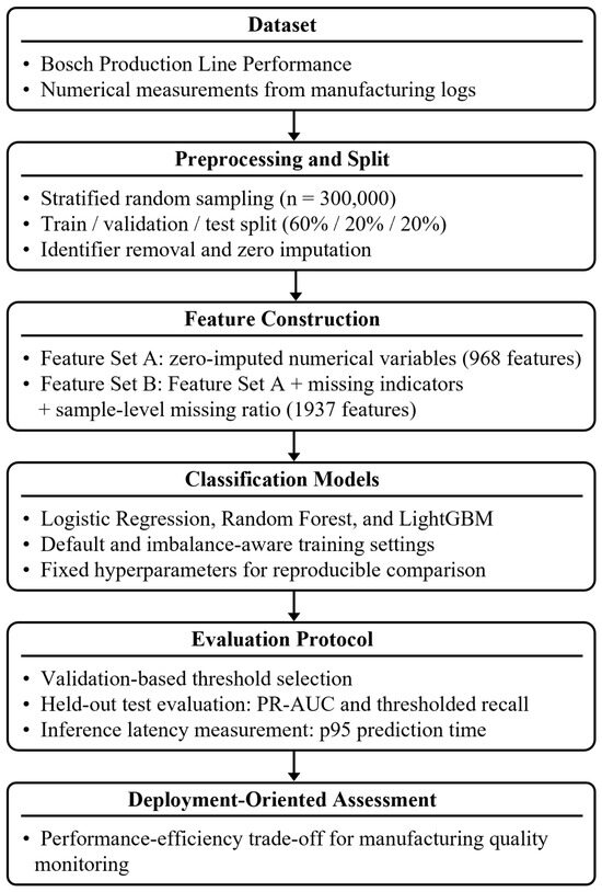
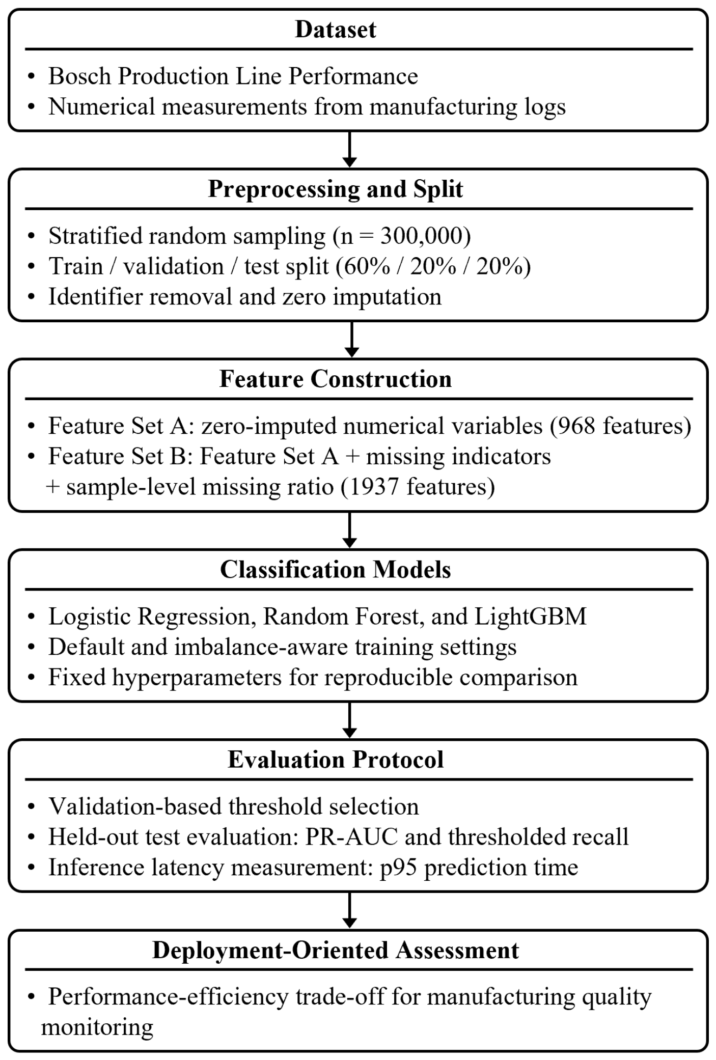
Figure 1 summarizes the workflow of the main Bosch experiment, including stratified sampling and splitting, feature construction, model training, validation-based threshold selection, held-out test evaluation, and latency analysis. The supplementary SECOM experiment followed the same validation-based evaluation protocol, with additional median and KNN imputation baselines as described in Section 4.2.

Figure 1. Overall workflow of the main Bosch validation-based experimental protocol, including data sampling and splitting, feature construction, model training, validation-based threshold selection, held-out test evaluation, and latency analysis.

4. Experimental Setup

This section summarizes the computing environment, data partitioning procedure, preprocessing rules, and implementation details used in the experiments. The purpose of this section is to make the experimental conditions explicit so that the reported comparisons can be interpreted as reproducible assessments of model behavior under the same data and system constraints.

4.1. System Configuration

All experiments were conducted on an Ubuntu 22.04.5 LTS workstation equipped with a 12th Gen Intel Core i9-12900 CPU, 24 logical CPU cores, and 64 GB of memory. The workstation was an HP Z2 Mini G9 Workstation (HP Inc., Palo Alto, CA, USA) and included an NVIDIA RTX A2000 12 GB GPU (NVIDIA Corporation, Santa Clara, CA, USA). GPU acceleration was not explicitly enabled in the experimental configuration, and the reported latency values therefore reflect the CPU-based prediction setting used in the experiments.

The software environment consisted of Python 3.10.12, NumPy 2.2.6, pandas 2.3.3, scikit-learn 1.7.2, and LightGBM 4.6.0. Logistic Regression and Random Forest were implemented using scikit-learn [22]. The gradient-boosting experiments were implemented using LightGBM [20]. The same software environment was used for all feature sets and model configurations.

4.2. Dataset Partitioning and Preprocessing

For the main Bosch experiment, the 300,000 sampled observations were divided into stratified training, validation, and test subsets using a 60:20:20 split with a fixed random seed of 42. The same partition was used for all Bosch feature configurations and classification models. This design ensures that observed performance differences can be attributed to feature representation and model choice rather than variation in the sampled data split.

For the Bosch experiment, preprocessing was applied consistently across all model configurations. The identifier column was removed before model training, and missing values in the numerical variables were replaced with zero. For Feature Set A, only the zero-imputed numerical variables were used. For Feature Set B, feature-wise missing indicators and a sample-level missing ratio were added before model training, following the missingness-aware design described in Section 3. No additional feature scaling was applied.

For the SECOM experiment, the same stratified train–validation–test protocol was used. The 1567 observations were split into 939 training, 314 validation, and 314 test samples. The corresponding numbers of defective samples were 62, 21, and 21. To address the concern that zero imputation may affect the results, three imputation strategies were compared on SECOM: zero, median, and KNN imputation. Missing indicators were generated before imputation so that the original missingness pattern was retained in Feature Set B. Imputation statistics were estimated from the training subset and then applied to the validation and test subsets.

4.3. Training and Evaluation Settings

Each model was trained and evaluated under the same partitioning and evaluation protocol. Logistic Regression, Random Forest, and LightGBM were evaluated under default and imbalance-aware settings. For Logistic Regression and Random Forest, the imbalance-aware setting used class_weight=‘balanced’, while LightGBM used is_unbalance=True. The model settings are summarized in Table 1.

Model scores on the held-out test data were used to compute PR-AUC. For the operating-point analysis, thresholds were selected on the validation set by identifying the highest recall satisfying $p_{\mathrm{val}}\ge 0.9$ and then applying the selected threshold once to the test set. Test precision, recall, and F1-score were then computed at the validation-selected operating threshold. Inference time was measured during prediction using a batch size of 1024. After five warm-up runs, 50 repeated prediction runs were performed, and the p95 latency was reported in milliseconds.

4.4. Summary of Experimental Settings

Table 2 summarizes the main experimental settings used in the Bosch experiment, including the dataset size, feature construction, imbalance-handling strategy, threshold rule, latency measurement procedure, and software environment.

Table 2. Summary of experimental settings and evaluation protocol.

Category	Setting
Dataset	Bosch Production Line Performance, numerical features
Sampling mode	Stratified random sample of 300,000 observations
Original feature dimension	968 numerical variables after removing the identifier column
Positive-class ratio	0.5810% (1743 defective observations)
Data split	60% training/20% validation/20% test, stratified
Training/validation/test size	180,000/60,000/60,000 observations
Defective observations	1046/348/349 in training/validation/test subsets
Random seed	42
Feature Set A	968 zero-imputed numerical variables
Feature Set B	968 zero-imputed variables + 968 missing indicators + sample-level missing ratio
Feature Set B dimension	1937 variables
Models	Logistic Regression, Random Forest, LightGBM
Imbalance handling	None; class-weighted LR/RF; is_unbalance=True for LightGBM
Threshold rule	Validation-selected threshold with maximum recall subject to $p_{\mathrm{val}}\ge 0.9$; fallback threshold = 0.5
Primary metrics	PR-AUC; test recall at validation-selected high-precision thresholds
Latency evaluation	Batch size 1024; 5 warm-up runs; 50 measured runs
Latency metric	p95 inference latency in milliseconds
Hardware	Intel Core i9-12900, 24 logical cores, 64 GB RAM
Software	Python 3.10.12, NumPy 2.2.6, pandas 2.3.3, scikit-learn 1.7.2, LightGBM 4.6.0

Table 3 summarizes the supplementary SECOM experiment, including the dataset size, preprocessing result, class distribution, feature dimensions, and imputation strategies. Table 1 lists the model-specific hyperparameter configuration. By documenting these settings, the experimental setup supports a transparent comparison of defect prediction models under class imbalance, missing information, and operational constraints.

Table 3. Summary of the supplementary SECOM experiment.

Category	Setting
Dataset	semiconductor manufacturing process (SECOM) dataset
Repository	UCI Machine Learning Repository
Original observations	1567
Feature dimension after preprocessing	474 process variables
Positive-class ratio	6.64% (104 defective observations)
Data split	60% training/20% validation/20% test, stratified
Training/validation/test size	939/314/314 observations
Defective observations	62/21/21 in training/validation/test subsets
Raw missing-value rate	5.54%
Feature Set A	Imputed process variables only
Feature Set B	Imputed variables + missing indicators + missing ratio
Feature Set B dimension	949 variables
Imputation strategies	Zero, median, and KNN imputation
Threshold rule	Validation-selected threshold with maximum recall subject to $p_{\mathrm{val}}\ge 0.9$

5. Results and Discussion

This section presents the experimental findings from three perspectives: overall minority-class discrimination, recall at validation-selected high-precision thresholds, and inference latency. The discussion focuses on how these results inform model selection for manufacturing quality monitoring rather than on benchmark ranking alone.

5.1. Overall Performance Comparison

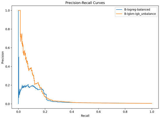
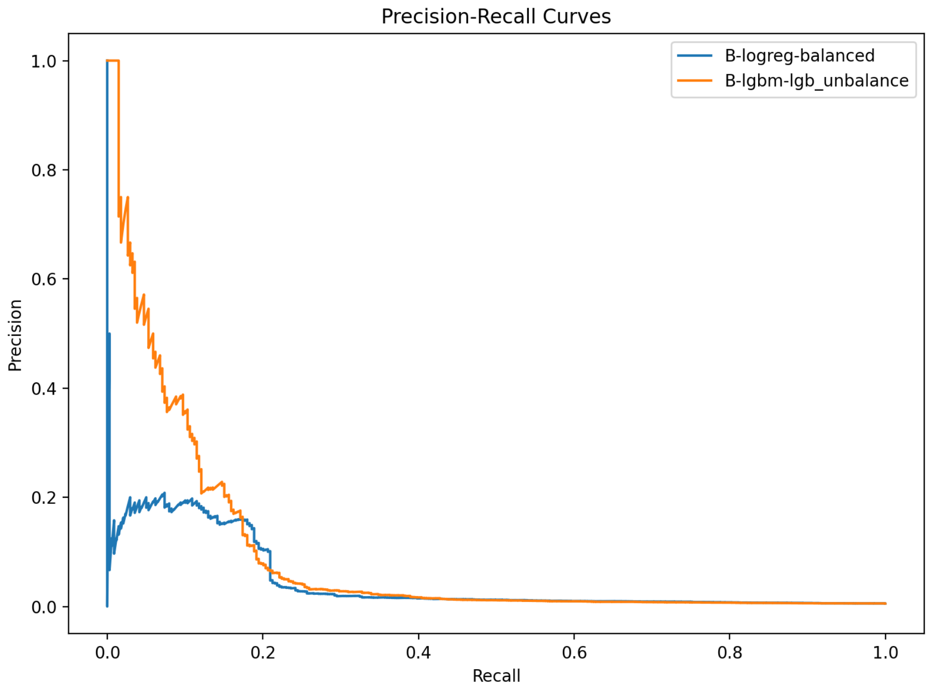
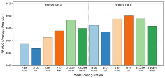
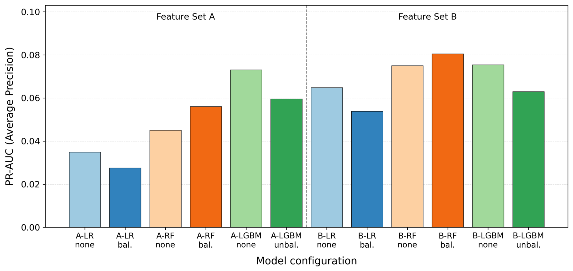
Figure 2 shows representative precision–recall curves for selected model configurations using Feature Set B, and Figure 3 summarizes PR-AUC for all feature sets and models. Overall, the results indicate that missingness-aware features improve ranking performance for rare-defect prediction.

Figure 2. Representative precision–recall curves for selected Feature Set B model configurations.

Figure 3. Comparison of PR-AUC performance across different models and feature sets. The two feature sets are separated by a dashed line.

In the Bosch experiment, adding the missing indicators and the missing-ratio feature increased PR-AUC in all model settings compared with using the imputed numerical variables alone. This suggests that the missingness pattern contains useful information that is not captured by zero-imputed numerical values alone. The highest PR-AUC is obtained by the class-weighted Random Forest with Feature Set B (0.0805), followed by the default LightGBM model with Feature Set B (0.0754). Logistic Regression shows lower PR-AUC values, which suggests that a linear decision boundary is not sufficient for the nonlinear structure of this equipment-log dataset.

From a manufacturing perspective, these results indicate that tree-based ensemble models are better suited to rare-defect ranking in high-dimensional process logs. At the same time, the improvement obtained from Feature Set B supports the practical value of retaining missingness information during feature construction. In this dataset, missing values appear to carry process-related information rather than acting only as random data loss.

5.2. Recall Under Validation-Selected High-Precision Constraints

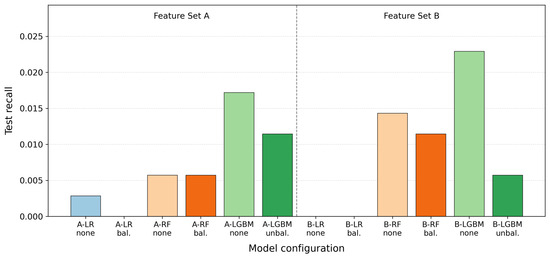
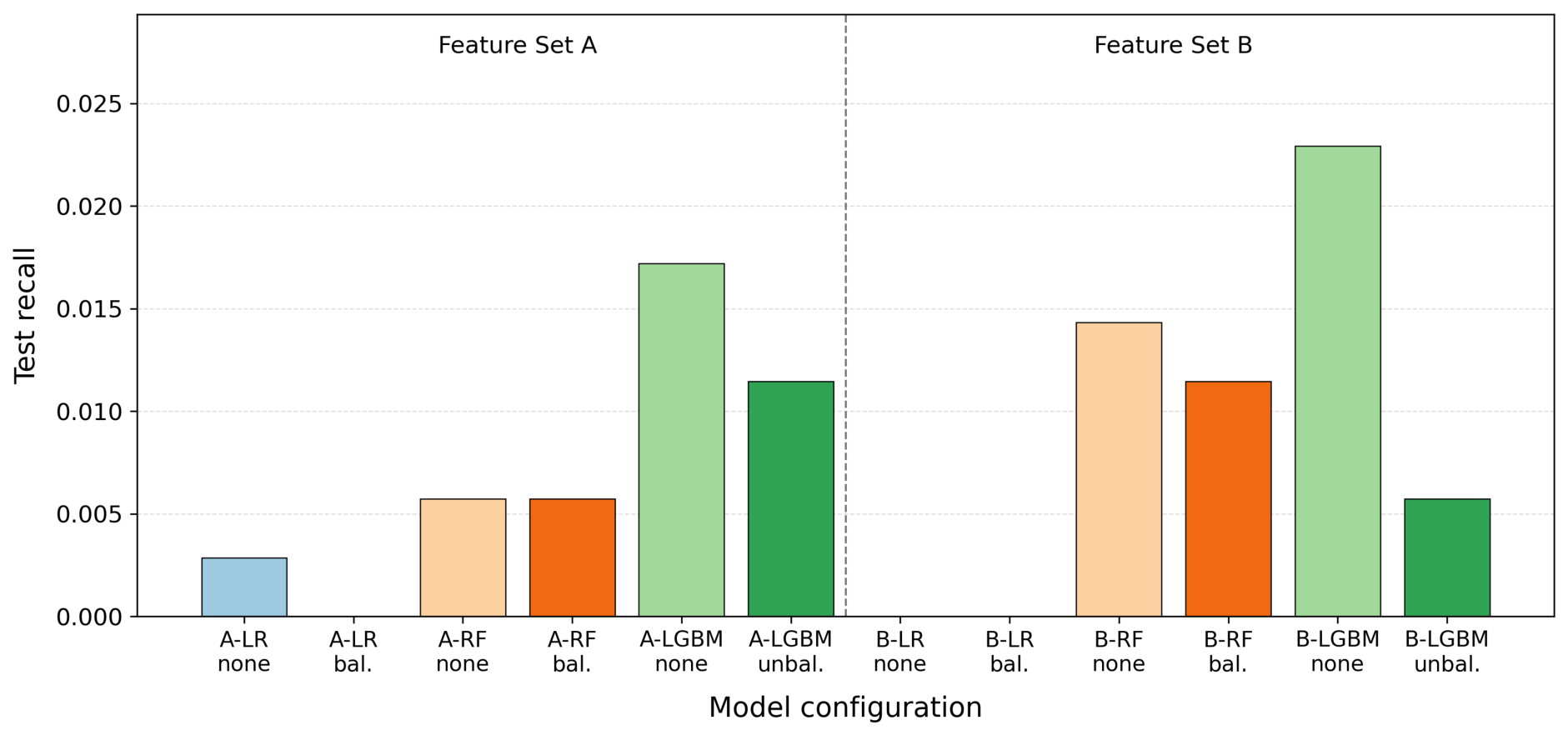
In production monitoring, too many false alarms can make a defect prediction model difficult to use, even when its overall ranking performance is strong. For this reason, Figure 4 reports test recall at thresholds selected on the validation set to satisfy $p_{\mathrm{val}}\ge 0.9$.

Figure 4. Test recall at thresholds selected on the validation set to satisfy $p_{\mathrm{val}}\ge 0.9$. The two feature sets are separated by a dashed line.

The thresholded recall results are less consistent than the PR-AUC results. Feature Set B improves recall for Random Forest and for the default LightGBM model, but the same pattern is not observed for all model and imbalance-handling combinations. The highest test recall is obtained by the default LightGBM model with Feature Set B (0.0229). In contrast, several Logistic Regression configurations produce near-zero recall under the conservative validation-selected threshold.

These results show why PR-AUC and thresholded recall should be interpreted separately. A model may rank defective samples relatively well but still detect only a small number of them after a strict operating threshold is applied. This issue is especially important under extreme class imbalance, where a threshold selected to maintain high precision on the validation set may not transfer perfectly to the test set.

5.3. Inference Latency and System Efficiency

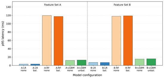
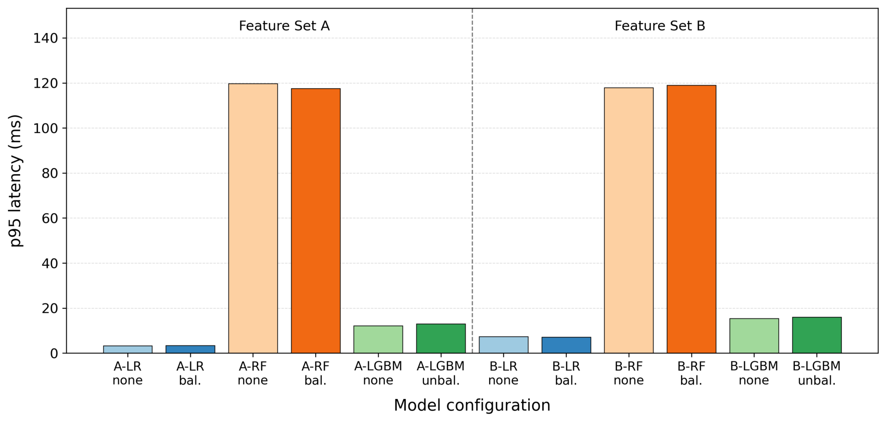
Figure 5 reports the p95 inference latency of the evaluated models. Latency is important in manufacturing monitoring because predictions must be available quickly enough to support inspection, intervention, or downstream decision making.

Figure 5. Comparison of p95 inference latency across classification models. The two feature sets are separated by a dashed line.

The latency results show a clear difference among the model families. Logistic Regression provides the lowest p95 latency, with prediction times of approximately 3–7 ms depending on the feature set. LightGBM shows moderate latency, approximately 12–16 ms. Random Forest is much slower, with p95 latency of approximately 118–120 ms. Therefore, the model with the best PR-AUC is not necessarily the most suitable model for time-sensitive monitoring.

5.4. Supplementary Validation on the SECOM Dataset

As a supplementary validation check, the same experimental framework was applied to the SECOM dataset. Unlike Bosch, SECOM is smaller and has a different missing-value structure, with 1567 observations, 474 process variables after preprocessing, and a positive-class ratio of 6.64%. The results are summarized in Table 4, which reports the best PR-AUC configuration for each imputation method and feature set.

Table 4. Supplementary validation results on the SECOM dataset. For each imputation method and feature set, the best PR-AUC configuration is reported.

Imputation	Feature Set	Best Model	Imbalance	PR-AUC	p95 Latency (ms)
Zero	A	LightGBM	none	0.2207	1.39
Zero	B	Random Forest	balanced	0.2033	116.68
Median	A	Random Forest	balanced	0.1947	113.38
Median	B	Random Forest	balanced	0.1955	116.07
KNN	A	LightGBM	none	0.1997	1.42
KNN	B	Random Forest	balanced	0.2168	110.53

The SECOM results show a more mixed pattern than the Bosch results. Feature Set B did not improve PR-AUC for all model configurations. However, the missingness-aware representation remained useful in several settings, especially when KNN imputation was combined with the class-weighted Random Forest model. Under this setting, Feature Set B achieved a PR-AUC of 0.2168, compared with the best Feature Set A result of 0.1997 under KNN imputation. With median imputation, Feature Set B also slightly improved the best Random Forest result. These findings suggest that the benefit of missingness-aware features is not limited to zero imputation, although it depends on the dataset, imputation method, and model family.

The SECOM experiment also highlights a limitation of strict high-precision threshold selection on small datasets. Because the validation and test sets contained only 21 defective samples each, the validation-selected threshold did not yield nonzero recall on the held-out test set. This result indicates that operating-point evaluation can be unstable when only a small number of defective samples are available. Therefore, the SECOM experiment is used primarily as a supplementary check of PR-AUC and imputation robustness rather than as a strong conclusion about thresholded recall.

5.5. Practical Implications for Manufacturing Deployment

The results suggest that model selection for manufacturing defect prediction should be treated as a multi-criteria decision. The class-weighted Random Forest with Feature Set B achieves the highest PR-AUC, so it is useful when the main objective is to rank defective samples ahead of normal samples. However, this model also has the highest inference latency, which may be problematic in production settings with strict response-time requirements.

LightGBM with Feature Set B provides a more balanced alternative. Its PR-AUC is slightly lower than that of the best Random Forest configuration, but it achieves the highest test recall at the validation-selected threshold and has much lower latency than Random Forest. Logistic Regression is attractive from a latency perspective, but its lower PR-AUC and limited thresholded recall make it less suitable when defect detection performance is the main requirement.

For a shop-floor monitoring system, the best model is therefore not simply the one with the highest score. The missing-data representation, the behavior at the selected threshold, and the response-time requirement should be considered together when selecting a model for deployment.

The supplementary SECOM results further indicate that missingness-aware features should not be assumed to be universally beneficial. Their effect can depend on the dataset, imputation strategy, and model family. This is important for deployment because the missing-value mechanism may differ across manufacturing lines. In practice, missingness-aware feature construction should therefore be evaluated as part of the modeling pipeline rather than treated as an automatic improvement.

Another deployment issue is that the validation-selected threshold assumes similar operating conditions between validation and test data. In a real shop-floor system, this assumption may be weakened by sensor degradation, maintenance actions, product-mix changes, or seasonal operating shifts. Under such domain shifts, both the missingness pattern and the score distribution may change. Periodic threshold recalibration or adaptive modeling may therefore be needed for long-term deployment.

6. Conclusions

This study evaluated defect prediction for manufacturing quality monitoring using equipment-log data with severe class imbalance and substantial missing information. The main experiment used the Bosch Production Line Performance dataset to compare Logistic Regression, Random Forest, and LightGBM under a common validation-based protocol. The evaluation focused on PR-AUC, test recall at validation-selected high-precision thresholds, and p95 inference latency.

The Bosch results show that explicit missingness representation improves PR-AUC across all model configurations. This suggests that missing values in manufacturing logs may provide useful process-related information rather than simply representing random data loss. However, the effect on thresholded recall is more model-dependent, which confirms that ranking performance and operating-point behavior can lead to different conclusions under rare-defect conditions.

The supplementary SECOM experiment extends the analysis to another industrial dataset and introduces median and KNN imputation baselines in addition to zero imputation. The SECOM results show that the benefit of missingness-aware features is not universal, but it can appear under non-zero imputation settings. This indicates that missingness-aware feature construction should be evaluated together with the imputation strategy and model family rather than assumed to improve all datasets automatically.

The comparison of models also shows a clear performance–efficiency trade-off. In the Bosch experiment, the class-weighted Random Forest with Feature Set B achieves the highest PR-AUC but requires substantially higher inference latency. LightGBM with Feature Set B provides a more balanced profile, combining competitive PR-AUC, the highest test recall at the validation-selected threshold, and moderate latency. Logistic Regression is the fastest model, but its defect-detection performance is limited.

Overall, the results suggest that a defect prediction model should be judged not only by how well it ranks defects, but also by whether it can operate within the timing and false-alarm limits of a real production line. Future work should extend this analysis in three directions: first, evaluating additional manufacturing datasets with different missing-value mechanisms; second, combining missingness-aware features with spatial–temporal models that capture process-stage and temporal dependencies; and third, studying adaptive threshold recalibration or domain adaptation under changing shop-floor conditions.

References

- Susto, G.A.; Schirru, A.; Pampuri, S.; McLoone, S.; Beghi, A. Machine Learning for Predictive Maintenance: A Multiple Classifier Approach. IEEE Trans. Ind. Inform. 2015, 11, 812–820. [Google Scholar]
- de Giorgio, A.; Cola, G.; Wang, L. Systematic review of class imbalance problems in manufacturing. J. Manuf. Syst. 2023, 71, 620–644. [Google Scholar] [CrossRef] [Scilit]
- He, H.; Garcia, E.A. Learning from Imbalanced Data. IEEE Trans. Knowl. Data Eng. 2009, 21, 1263–1284. [Google Scholar] [CrossRef] [Scilit]
- Saito, T.; Rehmsmeier, M. The Precision-Recall Plot Is More Informative than the ROC Plot When Evaluating Binary Classifiers on Imbalanced Datasets. PLoS ONE 2015, 10, e0118432. [Google Scholar] [CrossRef] [Scilit] [PubMed]
- Davis, J.; Goadrich, M. The relationship between Precision-Recall and ROC curves. In Proceedings of the 23rd International Conference on Machine Learning, Pittsburgh, PA, USA, 25–29 June 2006; pp. 233–240. [Google Scholar]
- Emmanuel, T.; Maupong, T.; Mpoeleng, D.; Semong, T.; Mphago, B.; Tabona, O. A survey on missing data in machine learning. J. Big Data 2021, 8, 140. [Google Scholar] [CrossRef] [Scilit] [PubMed]
- Ma, L.; Wang, M.; Peng, K. A missing manufacturing process data imputation framework for nonlinear dynamic soft sensor modeling and its application. Expert Syst. Appl. 2024, 237, 121428. [Google Scholar]
- Van Ness, M.; Bosschieter, T.M.; Halpin-Gregorio, R.; Udell, M. The Missing Indicator Method: From Low to High Dimensions. In Proceedings of the 29th ACM SIGKDD Conference on Knowledge Discovery and Data Mining, Long Beach, CA, USA, 6–10 August 2023; pp. 5004–5015. [Google Scholar]
- Gan, Q.; Gong, L.; Hu, D.; Jiang, Y.; Ding, X. A Hybrid Missing Data Imputation Method for Batch Process Monitoring Dataset. Sensors 2023, 23, 8678. [Google Scholar] [CrossRef] [Scilit] [PubMed]
- Bai, D.; Li, G.; Jiang, D.; Yun, J.; Tao, B.; Jiang, G.; Sun, Y.; Ju, Z. Surface defect detection methods for industrial products with imbalanced samples: A review of progress in the 2020s. Eng. Appl. Artif. Intell. 2024, 130, 107697. [Google Scholar]
- Kausik, A.K.; Rashid, A.B.; Baki, R.F.; Maktum, M.M.J. Machine learning algorithms for manufacturing quality assurance: A systematic review of performance metrics and applications. Array 2025, 26, 100393. [Google Scholar] [CrossRef] [Scilit]
- Bosch Production Line Performance. Available online: https://kaggle.com/competitions/bosch-production-line-performance (accessed on 11 November 2025).
- Lee, J.-S.; Yun, K.-C.; Park, J.K. Defect Detection of Scroll Fixed Using AI Machine Vision Inspection. Int. J. Precis. Eng. Manuf. 2024, 25, 2311–2319. [Google Scholar] [CrossRef] [Scilit]
- Ghosh, S.; Knoblauch, R.; El Mansori, M.; Corleto, C. Towards AI driven surface roughness evaluation in manufacturing: A prospective study. J. Intell. Manuf. 2024, 36, 4519–4548. [Google Scholar] [CrossRef] [Scilit]
- McDermott, M.B.; Zhang, H.; Hansen, L.H.; Angelotti, G.; Gallifant, J. A closer look at AUROC and AUPRC under class imbalance. In Proceedings of the 38th International Conference on Neural Information Processing Systems, Vancouver, BC, Canada, 10–15 December 2024; pp. 44102–44163. [Google Scholar]
- Wang, J.; Xiong, W.; Yao, L.; Jiang, X.; Cui, X.; Yu, W.; Young, B. GraphSiamese: Novel spatial-temporal slow feature fusion network for industrial process quality prediction. Appl. Soft Comput. 2026, 194, 114864. [Google Scholar]
- Yang, Z.; Gao, W.; Chen, G.; Yu, J.; He, B.; Ye, L. Self-Modified Dynamic Domain Adaptation for Industrial Soft Sensing. IEEE Trans. Autom. Sci. Eng. 2026, 23, 4679–4692. [Google Scholar] [CrossRef] [Scilit]
- UCI SECOM Dataset. Available online: https://archive.ics.uci.edu/dataset/179/secom (accessed on 14 June 2026).
- Breiman, L. Random Forests. Mach. Learn. 2001, 45, 5–32. [Google Scholar] [CrossRef] [Scilit]
- Ke, G.; Meng, Q.; Finley, T.; Wang, T.; Chen, W.; Ma, W.; Ye, Q.; Liu, T.-Y. LightGBM: A Highly Efficient Gradient Boosting Decision Tree. In Proceedings of the 31st International Conference on Neural Information Processing Systems, Long Beach, CA, USA, 4–9 December 2017; pp. 3149–3157. [Google Scholar]
- Chen, T.; Guestrin, C. XGBoost: A Scalable Tree Boosting System. In Proceedings of the 22nd ACM SIGKDD International Conference on Knowledge Discovery and Data Mining, San Francisco, CA, USA, 13–17 August 2016; pp. 785–794. [Google Scholar] [CrossRef] [Scilit]
- Pedregosa, F.; Varoquaux, G.; Gramfort, A.; Michel, V.; Thirion, B.; Grisel, O.; Blondel, M.; Prettenhofer, P.; Weiss, R.; Dubourg, V.; et al. Scikit-learn: Machine Learning in Python. J. Mach. Learn. Res. 2011, 12, 2825–2830. [Google Scholar]
Disclaimer/Publisher’s Note: The statements, opinions and data contained in all publications are solely those of the individual author(s) and contributor(s) and not of MDPI and/or the editor(s). MDPI and/or the editor(s) disclaim responsibility for any injury to people or property resulting from any ideas, methods, instructions or products referred to in the content. |
© 2026 by the authors. Licensee MDPI, Basel, Switzerland. This article is an open access article distributed under the terms and conditions of the Creative Commons Attribution (CC BY) license.