Dynamic Event-Triggered Consensus Formation Control Method for Multi-Leader UAVs with Communication Delay

Abstract

To address the problems of communication delay and waste of communication resources in the formation process of UAVs, a dynamic event-triggered formation control method for second-order multi-leader UAV systems with communication delay is studied. On the basis of considering the communication delay, a dynamic triggering mechanism is designed. By adjusting the triggering time in real time, the system can be more effectively controlled based on its current state. According to the control method, the mathematical models for the extended state observer, controller, and dynamic event-triggering function of the system have been established. Its stability is demonstrated by Lyapunov stability theory and linear matrix inequality theory, and Zeno behavior is excluded. The simulation results show that compared with the existing methods, the proposed method can avoid the dependence on the global information of the network topology, reduce the communication frequency, and effectively save communication resources.

1. Introduction

With the continuous development and progress of science and technology, UAVs exhibit strong maneuverability, low manufacturing costs, and minimal risk, making them widely utilized across various fields (Hu et al. [1]; Zeng et al. [2]). However, a single drone is unable to perform multiple complex tasks, such as ecological environment monitoring, target search and rescue, exploration, collaborative transportation, etc. (Yang et al. [3]; Chen et al. [4]; Javaid et al. [5]). The characteristics of formation control include high reliability, high autonomy, and strong expandability. Consequently, the application of UAV formation control in both civil and military fields has garnered significant attention (Xu et al. [6]; Wang et al. [7]; Zhou et al. [8]; Wu and Sun [9]). As a significant research direction in the field of control, the formation control of multiple UAVs has garnered substantial theoretical support and empirical results in recent years. In recent decades, researchers worldwide have proposed numerous formation control methods, including behavior-based formation control methods (Ge et al. [10]), virtual structure methods (Guo et al. [11]), leader–follower control methods (Zhao et al. [12]), and artificial potential field methods (Liu et al. [13]), among others.

Among these methods, the leader-follower control method is a widely used and effective strategy for the formation control of multi-UAV systems (Li [14]; Shi et al. [15]; Zhang et al. [16]). Most existing leader–follower approaches employ a single-leader architecture, which is vulnerable to single-point-of-failure problems. In contrast, a multi-leader architecture allows other leaders to continue maintaining the basic operations and stability of the system when a leader fails or experiences a communication interruption, significantly enhancing the system’s fault tolerance and robustness (Li et al. [17]).

The consensus method involves designing a control law grounded in consensus theory, such as one based on a distributed observer and a robust adaptive control approach. This method enables UAVs to share information with one another, ultimately achieving a consistent state (Zou and Shi [18]). Based on the four-rotor UAV model, Xue et al. [19] proposed a distributed cooperative formation control algorithm for UAVs, utilizing a three-dimensional spatial consistency strategy. Liu et al. [20] and Ni et al. [21] proposed a leader-based consensus control strategy to enable the multi-agent system to reach consensus within a fixed time interval. Based on graph theory, Liu et al. [22] have developed a method for multiple UAVs to form a formation using the leader-follower approach. The leader UAV guides the formation to the target position and manages the group using a consensus protocol to achieve coordinated control. Focusing on the cooperative control problem of linear multi-agent systems within a directed graph environment, Du et al. [23] successfully achieved consensus control of the system through a distributed event-triggered mechanism.

However, these methods typically rely on continuous communication and do not account for the impact of communication delay on the system, which limits their applicability in practical scenarios.

Communication delay is a critical factor in the formation control of multi-UAV systems. UAVs need to exchange information through the network to acquire each other’s state information. The communication delay will lead to the transmission delay of position information between UAVs, which will seriously compromise the uniformity and consistency of the formation (Yang et al. [24]; Yu et al. [25]; Tang et al. [26]; Li et al. [27]; Hou et al. [28]; Huang et al. [29]). These studies have investigated the consensus problem of second-order multi-agent systems with communication delays from various perspectives.

For uncertain and stochastic nonlinear multi-agent systems, Zhang and Peng [30] designed a leader-following consensus control method that accommodates time delays and switching network topologies. Ma et al. [31] proposed a time-varying formation tracking (TVFT) control protocol for multi-UAVs with a directional interaction topology and communication delay.

Nevertheless, existing delay-handling methods often assume fixed delays or do not integrate event-triggered mechanisms for communication efficiency.

To reduce unnecessary data transmission, the dynamic event-triggered mechanism has been introduced, which can effectively reduce the update frequency of the controller and minimize communication resources.

Du et al. [32] proposed a centralized event-triggered mechanism (CEM) to solve the leader-following consensus problem in multi-agent systems with general dynamics. Wang et al. [33] developed a comprehensive method combining controller and observer design under the dynamic event-triggered communication and control scheme. The method significantly reduces the utilization of communication resources while ensuring asymptotic convergence in the required form.

However, these works do not simultaneously address multi-leader architectures and communication delay, leaving a gap in the literature for methods that combine delay compensation with resource-efficient triggering in multi-leader UAV formations.

Table 1 summarizes the key differences between the proposed method and the closely related works.

Table 1. Comparison with closely related works.

Feature	Du et al. [23]	Wang et al. [33]	Proposed
Multi-leader architecture	No	No	Yes
Communication delay	No	No	Yes
Dynamic event triggering	No	Yes	Yes
Delay compensation in observer	N/A	No	Yes
Zeno behavior exclusion	Not discussed	Yes	Yes
Global topology info required	Yes	Partial	No

Compared with Du et al. [23], who proposed a distributed event-triggered consensus control method for general linear multi-agent systems without considering communication delay, the present work explicitly incorporates delay dynamics and designs a delay compensation term in the extended state observer. Compared with Wang et al. [33], who developed a dynamic event-triggered observer-based formation control method, the present work extends the framework to multi-leader architectures and addresses the combined challenges of communication delay and resource-efficient triggering.

In summary, the main contributions of this paper are as follows:

(1)

A dynamic event-triggered formation control method is proposed for second-order multi-leader UAV systems with communication delay, which eliminates the dependence on global network topology information.

(2)

An extended state observer with a delay compensation term is designed to accurately estimate the UAV states despite communication delays, providing reliable state feedback for the controller.

(3)

A dynamic event-triggering mechanism is introduced that adaptively adjusts the triggering instants based on the real-time system state, significantly reducing communication frequency compared with static triggering approaches. Zeno behavior is rigorously excluded.

2. Preparatory Knowledge

We use a directed graph $G=(V,E,A)$ to describe the communication network topology relationships in multi-UAV systems. Here, $V=\{v_1,v_2,\dots ,v_n\}$ is the node set and $E=\{(v_i,v_j)\mid v_i,v_j\in V\}$ is the edge set of the communication topology graph, respectively. $A=\left\{a_{ij}\right\}$ is an $N\times N$—dimensional adjacency matrix. If UAV i can receive the state information transmitted by UAV j, it indicates that there is a path from $v_j$ to $v_i$ in the communication network topology. If the drone i can receive the status information transmitted by the drone j, then we set $a_{ij}=1$; otherwise, $a_{ij}=0$. For a directed graph, the number of edges with $v_i$ as the parent node is the out-degree of node $v_i$, and the number of edges with $v_i$ as the child node is the in-degree of node $v_i$. D is used to represent the in-degree matrix of a directed graph with dimension N, and the elements on the diagonal are $d_{ii}={\sum }_{j=1}^N{a}_{ij},i=1,2,\dots ,N$, and the Laplacian matrix is $L=D-A$.

Lemma 1. 

Weighted form of Young’s inequality: Suppose a, b are nonnegative real numbers, $p>1$, ${\displaystyle \frac{1}{p}}+{\displaystyle \frac{1}{q}}=1$, then $ab\le \epsilon a^p+C\left(\epsilon \right)b^q$, where ε is arbitrarily small and $C\left(\epsilon \right)$ is arbitrarily large, and $C\left(\epsilon \right)={\displaystyle \frac{{\left(p\epsilon \right)}^{-\frac{q}{p}}}{q}}$.

Lemma 2. 

Schur complement lemma: For a given symmetric matrix $S=\left[\begin{array}{cc}{S}_{11}& S_{12}\\ S_{21}& S_{22}\end{array}\right]$, where $S_{11}$ is $r\times r$ dimensional. The following three statements are equivalent:

(1) 

$S<0$

(2) 

$S_{11}<0,S_{22}-S_{12}^T{S}_{11}^{-1}{S}_{12}<0$

(3) 

$S_{22}<0,S_{11}-S_{12}{S}_{22}^{-1}{S}_{12}^T<0$

Consider a multi-leader UAV system consisting of N UAVs, in which $G(G<N)$ UAVs are the leaders and the remaining UAVs are the followers. To facilitate the subsequent theoretical derivation, the leader subscript set is set to $H=\{1,2,\dots ,G\}$ and the follower subscript set is set to $H^{\prime }=\{G+1,G+2,\dots ,N\}$.

For a second-order continuous-time multi-UAV system with N UAVs, the dynamic model of the follower UAV i is described by the following second-order continuous-time integrator:

$$\left\{\begin{array}{c}{\dot{x}}_i\left(t\right)=v_i\left(t\right)\hfill \\ {\dot{v}}_i\left(t\right)=u_i\left(t\right)\hfill \end{array}\right.,i\in H^{\prime }$$

(1)

where, $x_i\left(t\right)\in {\mathbb{R}}^n$ represents the position vector of the UAV i, $v_i\left(t\right)\in {\mathbb{R}}^n$ represents the velocity vector of the UAV, and $u_i\left(t\right)$ is the control input of the follower.

If ${\xi }_i\left(t\right)={\left[\begin{array}{cc}{x}_i\left(t\right)& v_i\left(t\right)\end{array}\right]}^T$, the above model can be rewritten as the following matrix form:

$$\left\{\begin{array}{c}{\dot{\xi }}_i\left(t\right)=A{\xi }_i\left(t\right)+B{u}_i\left(t\right)\hfill \\ y_i\left(t\right)=C{\xi }_i\left(t\right)\hfill \end{array}\right.$$

(2)

where, $A=\left[\begin{array}{cc}0& I_n\\ 0& 0\end{array}\right],B=\left[\begin{array}{c}0\\ I_n\end{array}\right]$.

The leader has no control input, so the leaders’ control input is:

$$\left\{\begin{array}{c}{\dot{x}}_i\left(t\right)=v_i\left(t\right)\hfill \\ {\dot{v}}_i\left(t\right)=0\hfill \end{array}\right.,i\in H$$

(3)

$${\dot{\xi }}_i\left(t\right)=A{\xi }_i\left(t\right)$$

(4)

In this paper, the following assumptions and explanations are presented for this system:

Hypothesis 1. 

Leaders can only send information to followers and cannot receive information from followers in the opposite direction; the followers can obtain the information from any UAV, and each follower UAV has at least one path to obtain the leader information directly or indirectly.

Hypothesis 2. 

There is no delay when the leader acquires its own state information, and the communication delay is ignored. The information transmission between followers and followers has a communication delay that cannot be ignored. The Laplacian matrix corresponding to the system can be described as the following block form:

$$L=\left[\begin{array}{cc}{L}_1& L_2\\ 0& L_3\end{array}\right]$$

(5)

where, $L_1\in {\mathbb{R}}^{N\times N},L_2\in {\mathbb{R}}^{M\times (N-M)},L_3\in {\mathbb{R}}^{(N-M)\times (N-M)}$.

3. Dynamic Event Trigger Mechanism Design

Through the event-triggered mechanism, the information exchange between drones can be effectively improved to avoid unnecessary data being periodically sampled, thereby reducing the load of network transmission and saving network bandwidth.

In practice, states such as speed, may not be directly measured, so it is necessary to design a state observer for the system such that ${lim}_{t\to \infty }∥{\xi }_i\left(t\right)-{\widehat{\xi }}_i\left(t\right)∥=0$, where, the UAV’s own state is ${\xi }_i\left(t\right)={\left[\begin{array}{cc}{x}_i\left(t\right)& v_i\left(t\right)\end{array}\right]}^T$.

The basic form of the designed observer is:

$${\dot{\widehat{\xi }}}_i\left(t\right)=A{\widehat{\xi }}_i\left(t\right)+B{u}_i\left(t\right)+L\left(y_i\left(t\right)-C{\widehat{\xi }}_i\left(t\right)\right)+\Delta {\widehat{\xi }}_i\left(t\right)$$

(6)

where, $y_i\left(t\right)=C{\xi }_i\left(t\right)$, $\Delta {\widehat{\xi }}_i\left(t\right)$ is a time-delay compensation term, which is used to estimate the state change caused by communication delay. L is observer gain matrix.

$$\Delta {\widehat{\xi }}_i\left(t\right)=\sum _{j\in N_i}{a}_{ij}·\mathsf{\Gamma }\left({\widehat{\xi }}_j\left(t\right)-{\widehat{\xi }}_i(t-\tau \left(t\right))\right)$$

(7)

where, $\mathsf{\Gamma }$ is the delay compensation gain matrix that compensates for the delay by predicting the difference between the current state and the outdated state of the neighbor.

Define the observer error as $e_i={\xi }_i-{\widehat{\xi }}_i$. The error dynamics is:

$${\dot{e}}_i=(A-LC)e_i+\sum _{j\in N_i}{a}_{ij}\mathsf{\Gamma }\left(e_i\left(t\right)-e_j(t-\tau \left(t\right))\right)$$

(8)

The followers track the leader’s trajectory while maintaining the formation, and reduce communication frequency through the event trigger mechanism. Based on the above observer, a controller is proposed as follows:

$$u_i\left(t\right)=K{\displaystyle \sum _{j=1}^N}{w}_{ij}\left({\widehat{\xi }}_i(t-\tau \left(t\right))-{\widehat{\xi }}_j(t-\tau \left(t\right))\right)+K{\displaystyle \sum _{j=M+1}^N}{w}_{ij}\left({\widehat{\xi }}_i\left(t\right)-{\widehat{\xi }}_j\left(t\right)\right)$$

(9)

where, $K=\left[\begin{array}{cc}{k}_{11}& k_{12}\end{array}\right]$.

The state measurement error is defined as ${\widehat{e}}_i\left(t\right)={\widehat{\xi }}_i\left(t\right)-{\tilde{\xi }}_i\left(t\right)$. The event trigger mechanism is as follows:

$$\left\{\begin{array}{c}{t}_{k+1}^j=inf\{t>t_k^j\mid f_i\left(t\right)\ge 0\},\hfill \\ f_i\left(t\right)={\beta }_i{∥{\widehat{\xi }}_i\left(t\right)-{\tilde{\xi }}_i\left(t\right)∥}^2-{\gamma }_i{∥{\displaystyle {\sum }_{j=1}^N}{w}_{ij}\left({\widehat{\xi }}_i(t-\tau \left(t\right))-{\widehat{\xi }}_j(t-\tau \left(t\right))\right)+{\displaystyle {\sum }_{j=M+1}^N}{w}_{ij}\left({\widehat{\xi }}_i\left(t\right)-{\widehat{\xi }}_j\left(t\right)\right)∥}^2-{\alpha }_i{\chi }_i\left(t\right)\hfill \end{array}\right.$$

(10)

where, ${\beta }_i$ is the adjustment parameter, ${\alpha }_i$ and ${\kappa }_i>0$ ensure that the trigger condition is gradually tightened. The dynamic variable ${\chi }_i\left(t\right)$ satisfies the following conditions:

$${\dot{\chi }}_i\left(t\right)=-{\alpha }_i{\chi }_i\left(t\right)-{\kappa }_i({∥{\widehat{\xi }}_i\left(t\right)-{\tilde{\xi }}_i\left(t\right)∥}^2-{\gamma }_i{∥{\displaystyle \sum _{j=1}^N}{w}_{ij}\left({\widehat{\xi }}_i(t-\tau \left(t\right))-{\widehat{\xi }}_j(t-\tau \left(t\right))\right)+{\displaystyle \sum _{j=M+1}^N}{w}_{ij}\left({\widehat{\xi }}_i\left(t\right)-{\widehat{\xi }}_j\left(t\right)\right)∥}^2)$$

(11)

4. Stability Analysis and Proof

4.1. Correspondence Analysis

The observation error is defined as $e_i={\xi }_i\left(t\right)-{\widehat{\xi }}_i\left(t\right)$, and differentiating it gives:

$$\begin{array}{cc}\hfill {\dot{e}}_i\left(t\right)& ={\dot{\xi }}_i\left(t\right)-{\dot{\widehat{\xi }}}_i\left(t\right)\hfill \\ \hfill & =\left(A{\xi }_i\left(t\right)+B{u}_i\left(t\right)\right)-\left(A{\widehat{\xi }}_i\left(t\right)+B{u}_i\left(t\right)+L\left(y_i\left(t\right)-C{\xi }_i\left(t\right)\right)+\Delta {\widehat{\xi }}_i\left(t\right)\right)\hfill \\ \hfill & =A\left({\xi }_i\left(t\right)-{\widehat{\xi }}_i\left(t\right)\right)-L\left(C{\xi }_i\left(t\right)-C{\widehat{\xi }}_i\left(t\right)\right)-\Delta {\widehat{\xi }}_i\left(t\right)\hfill \end{array}$$

(12)

Substituting Equation (7) into Equation (12):

$$\begin{array}{cc}\hfill {\dot{e}}_i\left(t\right)& =(A-LC)e_i\left(t\right)-{\displaystyle \sum _{j=1}^N}{a}_{ij}\mathsf{\Gamma }\left({\widehat{\xi }}_j\left(t\right)-{\widehat{\xi }}_i(t-\tau \left(t\right))\right)\hfill \\ \hfill & =(A-LC)e_i\left(t\right)-{\displaystyle \sum _{j=1}^N}{a}_{ij}\mathsf{\Gamma }\left[\left({\xi }_j\left(t\right)-e_j\left(t\right)\right)-\left({\xi }_i(t-\tau \left(t\right))-e_i(t-\tau \left(t\right))\right)\right]\hfill \\ \hfill & =(A-LC)e_i\left(t\right)-{\displaystyle \sum _{j=1}^N}{a}_{ij}\mathsf{\Gamma }\left({\xi }_j\left(t\right)-{\xi }_i(t-\tau \left(t\right))\right)-{\displaystyle \sum _{j=1}^N}{a}_{ij}\mathsf{\Gamma }\left(e_j\left(t\right)-e_i(t-\tau \left(t\right))\right)\hfill \end{array}$$

(13)

According to the dynamic equation of the follower’s state, it is integrated:

Note that ${\widehat{\xi }}_j\left(t\right)={\xi }_j\left(t\right)-e_j\left(t\right)$ and ${\widehat{\xi }}_i(t-\tau \left(t\right))={\xi }_i(t-\tau \left(t\right))-e_i(t-\tau \left(t\right))$. Using the relation ${\xi }_j\left(t\right)-{\xi }_i(t-\tau \left(t\right))={\xi }_j\left(t\right)-{\xi }_i\left(t\right)+{\int }_{t-\tau \left(t\right)}^t(A{\xi }_i\left(s\right)+B{u}_i\left(s\right))ds$, and substituting the follower dynamics, the observer error can be expanded as:

$$\begin{array}{cc}\hfill {\dot{e}}_i\left(t\right)& =(A-LC)e_i\left(t\right)\hfill \\ \hfill & +{\displaystyle \sum _{j=1}^N}{a}_{ij}\mathsf{\Gamma }\left[\left({\widehat{\xi }}_j\left(t\right)-{\widehat{\xi }}_i\left(t\right)\right)+\left(e_j\left(t\right)-e_i\left(t\right)\right)-{\int }_{t-\tau \left(t\right)}^t\left(A{\xi }_j\left(s\right)+B{u}_j\left(s\right)-A{\xi }_i\left(s\right)-B{u}_i\left(s\right)\right)ds\right]\hfill \\ \hfill & -{\displaystyle \sum _{j=1}^N}{a}_{ij}\mathsf{\Gamma }\left(e_j\left(t\right)-e_i(t-\tau \left(t\right))\right)\hfill \\ \hfill & =(A-LC)e_i\left(t\right)+{\displaystyle \sum _{j=1}^N}{a}_{ij}\mathsf{\Gamma }\left(e_i\left(t\right)-e_j\left(t\right)\right)+{\displaystyle \sum _{j=1}^N}{a}_{ij}\mathsf{\Gamma }\left({\widehat{\xi }}_j\left(t\right)-{\widehat{\xi }}_i\left(t\right)\right)\hfill \\ \hfill & -{\displaystyle \sum _{j=1}^N}{a}_{ij}\mathsf{\Gamma }{\int }_{t-\tau \left(t\right)}^t\left(A({\xi }_j\left(s\right)-{\xi }_i\left(s\right))+B(u_j\left(s\right)-u_i\left(s\right))\right)ds-{\displaystyle \sum _{j=1}^N}{a}_{ij}\mathsf{\Gamma }\left(e_j\left(t\right)-e_i(t-\tau \left(t\right))\right)\hfill \end{array}$$

(14)

After using the properties of the Laplacian matrix in graph theory:

Under Hypothesis 1, the term ${\sum }_{j=1}^N{a}_{ij}\mathsf{\Gamma }({\widehat{\xi }}_j\left(t\right)-{\widehat{\xi }}_i\left(t\right))$ can be rewritten using the Laplacian matrix L as $-{\sum }_{j=1}^N{a}_{ij}{\sum }_{k=1}^N{L}_{jk}{\xi }_k\left(t\right)$. Applying this property yields:

$$\begin{array}{cc}\hfill {\dot{e}}_i\left(t\right)& =(A-LC)e_i\left(t\right)+{\displaystyle \sum _{j=1}^N}{a}_{ij}\mathsf{\Gamma }\left(e_i(t-\tau \left(t\right))-e_j\left(t\right)\right)-{\displaystyle \sum _{j=1}^N}{a}_{ij}{\displaystyle \sum _{k=1}^N}{L}_{jk}{\xi }_k\left(t\right)\hfill \\ \hfill & -{\displaystyle \sum _{j=1}^N}{a}_{ij}{\int }_{t-\tau \left(t\right)}^t\left[A{\displaystyle \sum _{k=1}^N}{L}_{jk}{\xi }_k\left(s\right)+BK{\displaystyle \sum _{k=1}^N}\left(w_{jk}-w_{ik}\right)\left({\widehat{\xi }}_k\left(s\right)-{\widehat{\xi }}_j\left(s\right)\right)+BK{\displaystyle \sum _{k=1}^N}{w}_{jk}\left({\widehat{\xi }}_j\left(s\right)-{\widehat{\xi }}_i\left(s\right)\right)\right]ds\hfill \end{array}$$

(15)

Under the assumption that the observer states converge to the true states, the integral terms involving the state differences over the delay interval $[t-\tau (t),t]$ are bounded by the observer error dynamics. As $t\to \infty$, these integral terms become higher-order infinitesimals relative to the dominant observer error terms. Consequently, the observer error dynamics reduce to:

After further simplification, the observer error dynamic equation is finally obtained:

$${\dot{e}}_i\left(t\right)=(A-LC)e_i\left(t\right)+{\displaystyle \sum _{j=1}^N}{a}_{ij}\mathsf{\Gamma }\left(e_i(t-\tau \left(t\right))-e_j\left(t\right)\right)$$

(16)

We construct a Lyapunov function with a time delay memory term:

$$V_e\left(t\right)={\displaystyle \sum _{i=1}^N}{e}_i^T\left(t\right)P{e}_i\left(t\right)+{\displaystyle \sum _{i=1}^N}{\int }_{t-\tau \left(t\right)}^t{e}_i^T\left(s\right)Q{e}_i\left(s\right)ds$$

(17)

where, $P,Q\in {\mathbb{R}}^{2n\times 2n}$ are symmetric positive definite matrices. $P>0,Q>0$. According to the differentiation rule and the Leibniz integral rule, the derivative of $V_e\left(t\right)$ can be obtained:

$$\begin{array}{cc}\hfill {\dot{V}}_e\left(t\right)& ={\displaystyle \sum _{i=1}^N}{\displaystyle \frac{d}{dt}}\left(e_i^T\left(t\right)P{e}_i\left(t\right)\right)+{\displaystyle \sum _{i=1}^N}{\displaystyle \frac{d}{dt}}{\int }_{t-\tau \left(t\right)}^t{e}_i^T\left(s\right)Q{e}_i\left(s\right)ds\hfill \\ \hfill & ={\displaystyle \sum _{i=1}^N}\left[{\dot{e}}_i^T\left(t\right)P{e}_i\left(t\right)+e_i^T\left(t\right)P{\dot{e}}_i\left(t\right)\right]+{\displaystyle \sum _{i=1}^N}\left[e_i^T\left(t\right)Q{e}_i\left(t\right)-\left(1-\dot{\tau }\left(t\right)\right)e_i^T\left(t-\tau \left(t\right)\right)Q{e}_i\left(t-\tau \left(t\right)\right)\right]\hfill \end{array}$$

(18)

Substituting Equation (16) into the first term of Equation (18):

$$\begin{array}{cc}\hfill {\dot{e}}_i^T\left(t\right)P{e}_i\left(t\right)+e_i^T\left(t\right)P{\dot{e}}_i\left(t\right)& ={\dot{e}}_i^T\left(t\right)\left[{(A-LC)}^{T}P+P(A-LC)\right]e_i\left(t\right)\hfill \\ \hfill & +{\displaystyle \sum _{j=1}^N}{a}_{ij}{e}_i^T\left(t-\tau \left(t\right)\right){\mathsf{\Gamma }}^{T}P{e}_i\left(t\right)-{\displaystyle \sum _{j=1}^N}{a}_{ij}{e}_j^T\left(t\right){\mathsf{\Gamma }}^{T}P{e}_i\left(t\right)\hfill \\ \hfill & +{\displaystyle \sum _{j=1}^N}{a}_{ij}{e}_i^T\left(t\right)P\mathsf{\Gamma }{e}_i\left(t-\tau \left(t\right)\right)-{\displaystyle \sum _{j=1}^N}{a}_{ij}{e}_i^T\left(t\right)P\mathsf{\Gamma }{e}_j\left(t\right)\hfill \end{array}$$

(19)

The cross term is scaled by Young inequality $2ab\le ϵa^2+{ϵ}^{-1}{b}^2,ϵ>0$:

$${\displaystyle -{\displaystyle \sum _{j=1}^N}{a}_{ij}{e}_i^T\left(t\right)P\mathsf{\Gamma }{e}_j\left(t\right)\le \frac{1}{2}{\displaystyle \sum _{j=1}^N}{a}_{ij}\left(ϵe_i^T\left(t\right)P\mathsf{\Gamma }{\mathsf{\Gamma }}^{T}P{e}_i\left(t\right)+{ϵ}^{-1}{e}_i^T\left(t-\tau \left(t\right)\right)e_i\left(t-\tau \left(t\right)\right)\right)}$$

(20)

Substituting Equation (20) into Equation (19) and simplifying, we obtain:

$$\begin{array}{cc}\hfill {\dot{e}}_i^T\left(t\right)P{e}_i\left(t\right)+e_i^T\left(t\right)P{\dot{e}}_i\left(t\right)& \le e_i^T\left(t\right)\left[{(A-LC)}^{T}P+P(A-LC)+Q+2{\displaystyle \sum _{j=1}^N}{a}_{ij}P\mathsf{\Gamma }+{\displaystyle \sum _{j=1}^N}{a}_{ij}ϵP\mathsf{\Gamma }{\mathsf{\Gamma }}^{T}P\right]e_i\left(t\right)\hfill \\ \hfill & +{\displaystyle \sum _{i=1}^N}\left[-(1-\mu )Q+{\displaystyle \sum _{j=1}^N}{a}_{ij}{ϵ}^{-1}I\right]e_i^T\left(t-\tau \left(t\right)\right)e_i\left(t-\tau \left(t\right)\right)\hfill \end{array}$$

(21)

where, $\mu ={sup}_t\dot{\tau }\left(t\right)<1$. Substituting Equation (21) into Equation (18) and simplifying yields:

$$\begin{array}{cc}\hfill {\dot{V}}_e\left(t\right)& \le {\displaystyle \sum _{i=1}^N}{e}_i^T\left(t\right)\left[{(A-LC)}^{T}P+P(A-LC)+Q+2{\displaystyle \sum _{j=1}^N}{a}_{ij}\mathsf{\Gamma }+{\displaystyle \sum _{j=1}^N}{a}_{ij}ϵ\mathsf{\Gamma }{\mathsf{\Gamma }}^{T}P\right]e_i\left(t\right)\hfill \\ \hfill & +{\displaystyle \sum _{i=1}^N}\left[-(1-\mu )Q+{\displaystyle \sum _{j=1}^N}{a}_{ij}{ϵ}^{-1}I\right]e_i^T\left(t-\tau \left(t\right)\right)e_i\left(t-\tau \left(t\right)\right)\hfill \\ \hfill & +{\displaystyle \sum _{i=1}^N}{e}_i^T\left(t\right)Q{e}_i\left(t\right)-{\displaystyle \sum _{i=1}^N}\left(1-\dot{\tau }\left(t\right)\right)e_i^T\left(t-\tau \left(t\right)\right)Q{e}_i\left(t-\tau \left(t\right)\right)\hfill \\ \hfill & ={\displaystyle \sum _{i=1}^N}{e}_i^T\left(t\right)\left[{(A-LC)}^{T}P+P(A-LC)+2Q+2{\displaystyle \sum _{j=1}^N}{a}_{ij}\mathsf{\Gamma }+{\displaystyle \sum _{j=1}^N}{a}_{ij}ϵ\mathsf{\Gamma }{\mathsf{\Gamma }}^{T}P\right]e_i\left(t\right)\hfill \\ \hfill & +{\displaystyle \sum _{i=1}^N}\left[-(1-\mu )Q+{\displaystyle \sum _{j=1}^N}{a}_{ij}{ϵ}^{-1}I-\left(1-\dot{\tau }\left(t\right)\right)Q\right]e_i^T\left(t-\tau \left(t\right)\right)e_i\left(t-\tau \left(t\right)\right)\hfill \end{array}$$

(22)

Since $\dot{\tau }\left(t\right)\le \mu$, then

$$\begin{array}{cc}\hfill -(1-\mu )Q+{\displaystyle \sum _{j=1}^N}{a}_{ij}{ϵ}^{-1}I-\left(1-\dot{\tau }\left(t\right)\right)Q& \le -(1-\mu )Q+{\displaystyle \sum _{j=1}^N}{a}_{ij}{ϵ}^{-1}I-(1-\mu )Q\hfill \\ \hfill & ={\displaystyle \sum _{j=1}^N}{a}_{ij}{ϵ}^{-1}I-2(1-\mu )Q\hfill \end{array}$$

(23)

After further collation, let:

$$\left\{\begin{array}{c}{M}_1={(A-LC)}^{T}P+P(A-LC)+2Q+2{\displaystyle {\sum }_{j=1}^N}{a}_{ij}P\mathsf{\Gamma }+{\displaystyle {\sum }_{j=1}^N}{a}_{ij}ϵP\mathsf{\Gamma }{\mathsf{\Gamma }}^{T}P\hfill \\ M_2={\displaystyle {\sum }_{j=1}^N}{a}_{ij}{ϵ}^{-1}I-2(1-\mu )Q\hfill \end{array}\right.$$

(24)

There are:

$${\dot{V}}_e\left(t\right)\le {\displaystyle \sum _{i=1}^N}{e}_i^T\left(t\right)M_1{e}_i\left(t\right)+{\displaystyle \sum _{i=1}^N}{e}_i^T\left(t-\tau \left(t\right)\right)M_2{e}_i\left(t-\tau \left(t\right)\right)$$

(25)

In order to make ${\dot{V}}_e\left(t\right)\le -\lambda {∥\mathit{e}\left(t\right)∥}^2(\lambda >0)$, the matrix is required:

$${\displaystyle \left\{\begin{array}{c}{M}_1={(A-LC)}^{T}P+P(A-LC)+2Q+2{\displaystyle {\sum }_{j=1}^N}{a}_{ij}P\mathsf{\Gamma }+{\displaystyle {\sum }_{j=1}^N}{a}_{ij}ϵP\mathsf{\Gamma }{\mathsf{\Gamma }}^{T}P<0\hfill \\ M_2={\displaystyle {\sum }_{j=1}^N}{a}_{ij}{ϵ}^{-1}I-2(1-\mu )Q<0\hfill \end{array}\right.}$$

(26)

Let $X=P^{-1},Y=LX,Z=\mathsf{\Gamma }X$.

According to Schur complement lemma and matrix operation properties, and equivalent transformation:

$$\begin{array}{cc}\hfill & X{(A-LC)}^{T}PX+XP(A-LC)X+2XQX+2{\displaystyle \sum _{j=1}^N}{a}_{ij}XP\mathsf{\Gamma }X+{\displaystyle \sum _{j=1}^N}{a}_{ij}XP\mathsf{\Gamma }{\mathsf{\Gamma }}^{T}PX<0\hfill \\ \hfill & X{A}^{T}X-Y^T{C}^{T}X+XAX-XCY+2XQX+2{\displaystyle \sum _{j=1}^N}{a}_{ij}Z+2{\displaystyle \sum _{j=1}^N}{a}_{ij}ϵZ{Z}^T<0\hfill \end{array}$$

(27)

For $M_2={\sum }_{j=1}^N{a}_{ij}{ϵ}^{-1}I-2(1-\mu )Q<0$, multiply $Q^{-1}$ on both sides at the same time, let $W=Q^{-1}$:

$${\displaystyle \sum _{j=1}^N}{a}_{ij}{ϵ}^{-1}W<2(1-\mu )I$$

(28)

Solving through Linear Matrix Inequalities (LMI), we can obtain $P=X^{-1}$, $\mathsf{\Gamma }=Z{X}^{-1}$, $L=Y{X}^{-1},Q=W^{-1}$. According to Lyapunov stability theory, there exist positive constants $\alpha ,\beta$, such that $\alpha {∥\mathit{e}\left(t\right)∥}^2\le V_e\left(t\right)\le \beta {∥\mathit{e}\left(t\right)∥}^2$. And since ${\dot{V}}_e\left(t\right)\le -\lambda {∥\mathit{e}\left(t\right)∥}^2$, it can be obtained that $e_i\left(t\right)$ is always uniformly bounded, that is, ${lim\; sup}_{t\to \infty }∥e_i\left(t\right)∥\le \sqrt{{\displaystyle \frac{\beta }{\alpha }}}$.

Define the tracking error $e_i^{track}\left(t\right)={\xi }_i^l\left(t\right)-{\widehat{\xi }}_i\left(t\right)$, combined with the leader dynamic ${\dot{\xi }}_i^l\left(t\right)=A{\xi }_i^l\left(t\right)(i\in H^{\prime })$, as well as the observer and controller model, the tracking error dynamic equation is derived:

$$\begin{array}{cc}\hfill {\dot{e}}_i^{track}\left(t\right)& ={\dot{\xi }}_i^l\left(t\right)-{\dot{\widehat{\xi }}}_i\left(t\right)=A{\xi }_i^l\left(t\right)-\left(A{\widehat{\xi }}_i\left(t\right)+B{u}_i\left(t\right)+L(y_i\left(t\right)-C{\widehat{\xi }}_i\left(t\right))+\Delta {\widehat{\xi }}_i\left(t\right)\right)\hfill \\ \hfill & =A{e}_i^{track}\left(t\right)-BK{\displaystyle \sum _{j=1}^N}{w}_{ij}\left((e_i(t-\tau \left(t\right))-e_j\left(t\right))+(e_i\left(t\right)-e_j\left(t\right))\right)-LC{e}_i\left(t\right)-\Delta {\widehat{\xi }}_i\left(t\right)\hfill \end{array}$$

(29)

The Lyapunov functional of tracking error is constructed:

$$V_{track}\left(t\right)={\displaystyle \sum _{i=1}^N}{e}_i^{trac{k}^T}\left(t\right)P_c{e}_i^{track}\left(t\right)+{\displaystyle \sum _{i=1}^N}{\int }_{t-\tau \left(t\right)}^t{e}_i^{trac{k}^T}\left(s\right)Q_c{e}_i^{track}\left(s\right)ds$$

(30)

where, $P_c>0,Q_c>0$. The derivation of $V_{\mathrm{track}}\left(t\right)$ has been obtained:

$$\begin{array}{cc}\hfill {\dot{V}}_{\mathrm{track}}\left(t\right)& ={\displaystyle \sum _{i=1}^N}\left[{\dot{e}}_i^{{\mathrm{track}}^T}\left(t\right)P_c{e}_i^{\mathrm{track}}\left(t\right)+e_i^{{\mathrm{track}}^T}\left(t\right)P_c{\dot{e}}_i^{\mathrm{track}}\left(t\right)\right]\hfill \\ \hfill & +{\displaystyle \sum _{i=1}^N}\left[e_i^{{\mathrm{track}}^T}\left(t\right)Q_c{e}_i^{\mathrm{track}}\left(t\right)-\left(1-\dot{\tau }\left(t\right)\right)e_i^{{\mathrm{track}}^T}\left(t-\tau \left(t\right)\right)Q_c{e}_i^{\mathrm{track}}\left(t-\tau \left(t\right)\right)\right]\hfill \end{array}$$

(31)

Substituting Equation (29) into Equation (31). Using the boundedness of the observer error A, combined with Young’s inequality, the cross term is scaled:

$$\begin{array}{cc}\hfill & {\displaystyle \sum _{i=1}^N}{\dot{e}}_i^{{\mathrm{track}}^T}\left(t\right)P_c{e}_i^{\mathrm{track}}\left(t\right)+e_i^{{\mathrm{track}}^T}\left(t\right)P_c{\dot{e}}_i^{\mathrm{track}}\left(t\right)\hfill \\ \hfill & \le {\displaystyle \sum _{i=1}^N}{e}_i^{{\mathrm{track}}^T}\left(t\right)\left[A^T{P}_c+P_{c}A+Q_c+{\delta }_{1}I\right]e_i^{\mathrm{track}}\left(t\right)\hfill \\ \hfill & +{\displaystyle \sum _{i=1}^N}{\displaystyle \sum _{j=1}^N}{w}_{ij}\left({\delta }_2{e}_i^{{\mathrm{track}}^T}\left(t\right)BK{K}^T{B}^T{e}_i^{\mathrm{track}}\left(t\right)+{\delta }_2^{-1}{\left(e_i(t-\tau \left(t\right))-e_j\left(t\right)\right)}^2+{\delta }_2^{-1}{\left(e_i\left(t\right)-e_j\left(t\right)\right)}^2\right)\hfill \\ \hfill & +{\displaystyle \sum _{i=1}^N}{e}_i^{{\mathrm{track}}^T}\left(t\right)LC{C}^T{L}^T{e}_i^{\mathrm{track}}\left(t\right)+{\displaystyle \sum _{i=1}^N}{ϵ}_i{e}_i^{{\mathrm{track}}^T}\left(t\right)P_c\Delta {\widehat{\xi }}_i\left(t\right)\Delta {\widehat{\xi }}_i^T\left(t\right)P_c+{ϵ}_1^{-1}{e}_i^{{\mathrm{track}}^T}\left(t\right)e_i^{\mathrm{track}}\left(t\right)\hfill \end{array}$$

(32)

where, ${\delta }_1,{\delta }_2,{ϵ}_1>0$ are properly selected constants.

Substituting Equation (32) into Equation (31). After simplification, we obtain:

$$\begin{array}{cc}\hfill {\dot{V}}_{\mathrm{track}}\left(t\right)& \le {\displaystyle \sum _{i=1}^N}{e}_i^{{\mathrm{track}}^T}\left(t\right)\left[A^T{P}_c+P_{c}A+Q_c+{\delta }_{1}I+{\displaystyle \sum _{j=1}^N}{w}_{ij}{\delta }_{2}BK{K}^T{B}^T+LC{C}^T{L}^T\right]e_i^{\mathrm{track}}\left(t\right)\hfill \\ \hfill & +{\displaystyle \sum _{i=1}^N}{\displaystyle \sum _{j=1}^N}{w}_{ij}{\delta }_2^{-1}\left[{\left(e_i(t-\tau \left(t\right))-e_j\left(t\right)\right)}^2+{\left(e_i\left(t\right)-e_j\left(t\right)\right)}^2\right]\hfill \\ \hfill & +{\displaystyle \sum _{i=1}^N}\left[-(1-\mu )Q_c+{ϵ}_1{P}_c\Delta {\widehat{\xi }}_i\left(t\right)\Delta {\widehat{\xi }}_i^T\left(t\right)P_c+{ϵ}_1^{-1}I\right]e_i^{{\mathrm{track}}^T}\left(t-\tau \left(t\right)\right)e_i^{\mathrm{track}}\left(t-\tau \left(t\right)\right)\hfill \end{array}$$

(33)

By appropriately selecting $P_c,Q_c,{\delta }_1,{\delta }_2,{ϵ}_1$, it is possible to achieve:

$$\left\{\begin{array}{c}{A}^T{P}_c+P_{c}A+Q_c+{\delta }_{1}I+{\displaystyle {\sum }_{j=1}^N}{w}_{ij}{\delta }_{2}BK{K}^T{B}^T+LC{C}^T{L}^T<0\hfill \\ -(1-\mu )Q_c+{ϵ}_1{P}_c\Delta {\widehat{\xi }}_i\left(t\right)\Delta {\widehat{\xi }}_i^T\left(t\right)P_c+{ϵ}_1^{-1}I<0\hfill \end{array}\right.$$

(34)

It can be proven that the tracking error $e_i^{\mathrm{track}}$ is ultimately bounded, that is, ${lim\; sup}_{t\to \infty }∥{\mathit{e}}_i^{\mathrm{track}}\left(t\right)∥\le \mathsf{\Theta }$ is a constant).

4.2. Zeno Behavior Exclusion

Assume that there is a Zeno behavior, that is, there is a time point T and a positive integer sequence $m\to \infty$, such that when $m\to \infty ,t_{k_m}^i\to T$.

According to the dynamic event trigger condition Equations (10) and (11), at the re-triggering time $t_k^i$, we have $f_i\left(t_k^i\right)=0$. Between two consecutive triggering times, $t_k^i$ and $t_{k+1}^i$, the trigger condition is not satisfied, that is, $f_i\left(t\right)<0$.

Considering the dynamics in Equation (11) of the dynamic variables, at the trigger time $t_k^i$, we have:

$${\beta }_i{∥{\widehat{\xi }}_i\left(t_k^i\right)-{\tilde{\xi }}_i\left(t_k^i\right)∥}^2={\gamma }_i{∥{\displaystyle \sum _{j=1}^N}{w}_{ij}\left({\widehat{\xi }}_j(t_k^i-\tau \left(t_k^i\right))-{\tilde{\xi }}_i(t_k^i-\tau \left(t_k^i\right))\right)+{\displaystyle \sum _{j=M+1}^N}{w}_{ij}\left({\widehat{\xi }}_j\left(t_k^i\right)-{\tilde{\xi }}_i\left(t_k^i\right)\right)∥}^2+{\alpha }_i{\chi }_i\left(t_k^i\right)$$

(35)

Between two consecutive triggering times, $t_k^i$ and $t_{k+1}^i$, the trigger condition is not satisfied, that is:

$${\beta }_i{∥{\widehat{\xi }}_i\left(t\right)-{\tilde{\xi }}_i\left(t\right)∥}^2<{\gamma }_i{∥{\displaystyle \sum _{j=1}^N}{w}_{ij}\left({\widehat{\xi }}_j(t-\tau \left(t\right))-{\tilde{\xi }}_i(t-\tau \left(t\right))\right)+{\displaystyle \sum _{j=M+1}^N}{w}_{ij}\left({\widehat{\xi }}_j\left(t\right)-{\tilde{\xi }}_i\left(t\right)\right)∥}^2+{\alpha }_i{\chi }_i\left(t_k^i\right)$$

(36)

Considering the dynamic equation of the dynamic variable ${\chi }_i\left(t\right)$, within the time interval $\left[t_k^i,t_{k+1}^i\right)$, there is:

$${\chi }_i\left(t_{k+1}^i\right)={\chi }_i\left(t_k^i\right)+{\int }_{t_k^i}^{t_{k+1}^i}\left[\begin{array}{c}-{\alpha }_i{\chi }_i\left(s\right)-{\kappa }_i{∥{\widehat{\xi }}_i\left(s\right)-{\tilde{\xi }}_i\left(s\right)∥}^2\\ -{\gamma }_i{∥{\displaystyle {\sum }_{j=1}^N}{w}_{ij}\left({\widehat{\xi }}_j(s-\tau \left(s\right))-{\tilde{\xi }}_i(s-\tau \left(s\right))\right)+{\displaystyle {\sum }_{j=M+1}^N}{w}_{ij}\left({\widehat{\xi }}_j\left(s\right)-{\tilde{\xi }}_i\left(s\right)\right)∥}^2\end{array}\right]ds$$

(37)

In order to analyze the behavior near the time point T, a very small time interval $\epsilon >0$ is considered, and the interval $[T-\epsilon ,T)$ is defined to study the system’s behavior in this interval.

Assuming the existence of Zeno behavior, that is, when $m\to \infty ,t_{k_m}^i\to T$. In the interval $\left[T-\epsilon ,T\right)$, the trigger condition is frequently satisfied, resulting in frequent updates of ${\chi }_i\left(t\right)$.

At each triggering instant $t_k^i$, the measurement error $\parallel {\widehat{\xi }}_i\left(t_k^i\right)-{\tilde{\xi }}_i\left(t_k^i\right)\parallel$ is reset to zero, while the dynamic variable ${\chi }_i\left(t\right)$ satisfies:

$${\dot{\chi }}_i\left(t\right)=-{\alpha }_i{\chi }_i\left(t\right)-{\kappa }_i\left(\parallel {\widehat{\xi }}_i\left(t\right)-{\tilde{\xi }}_i{\left(t\right)\parallel }^2-{\gamma }_i{∥{\displaystyle \sum _{j=1}^N}{w}_{ij}({\widehat{\xi }}_i(t-\tau \left(t\right))-{\widehat{\xi }}_j(t-\tau \left(t\right)))+{\displaystyle \sum _{j=M+1}^N}{w}_{ij}({\widehat{\xi }}_i\left(t\right)-{\widehat{\xi }}_j\left(t\right))∥}^2\right)$$

Since the inter-event intervals $t_{k+1}^i-t_k^i\to 0$ as $m\to \infty$, and the measurement error is bounded (hence the squared norm terms are non-negative), the term $-{\alpha }_i{\chi }_i\left(t\right)$ drives ${\chi }_i\left(t\right)$ toward $-\infty$ without sufficient positive contributions to counterbalance. Specifically, integrating from $T-\epsilon$ to T:

$${\chi }_i\left(T\right)\le {\chi }_i(T-\epsilon )e^{-{\alpha }_i\epsilon }-{\kappa }_i{\int }_{T-\epsilon }^T(\cdots )ds\to -\infty$$

as $m\to \infty$, since the integral accumulates infinitely many non-negative terms.

However, according to the above integral equation, it can be proved that the dynamic variable ${\chi }_i\left(t\right)$ tends to be negative infinity within this time interval. This is in contradiction with the boundedness assumption of the system, which states that the system’s state cannot increase or decrease indefinitely. Therefore, Zeno behavior does not exist.

5. Simulation Results and Analysis

5.1. Initial Conditions and Parameters

This section performs a feasibility simulation experiment on a multi-UAV system. There are six UAVs in the multi-UAV system: UAV No. 1, UAV No. 2, and UAV No. 3 are the leaders in the system, and the remaining three UAVs are follower UAVs.

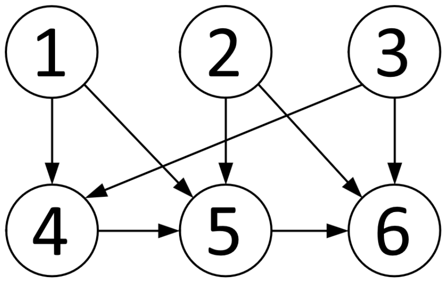
The communication topology of the studied system is shown in Figure 1.

Figure 1. System communication topology diagram.

From the communication topology diagram of Figure 1, the Laplacian matrix block matrix can be obtained as follows:

$$\begin{array}{c}{L}_1=\left[\begin{array}{ccc}1& 0& 0\\ 0& 2& 0\\ 0& 0& 2\end{array}\right],\hspace{1em}\hspace{1em}\hspace{1em}{L}_2=\left[\begin{array}{ccc}-1& 0& 0\\ -1& -1& -1\\ -1& 0& -1\end{array}\right],\hfill \\ L_3=\left[\begin{array}{ccc}1& -1& 0\\ 0& 1& -1\\ 0& 0& 0\end{array}\right].\hfill \end{array}$$

Table 2 shows the three-dimensional initial state of the UAV.

Table 2. Three-dimensional initial state of UAV.

UAV	Position/m			Velocity/(m/s)
Number	East	North	Vertical	East	North	Vertical
1	−6	3	−0.5	0.5	0.2	−0.1
2	2	6	0.5	0.3	−0.4	0.2
3	4	3	1.5	−0.2	0.3	0.3
4	−3	−2	−1	0.4	0.1	−0.2
5	2	4	0	−0.3	0.5	0.1
6	4	−3	−2	0.2	−0.2	0.4

The controller gain matrix K is designed through robust pole placement to distribute the closed-loop poles in the left half-plane while suppressing disturbances. Specifically, the poles are placed at $s=-1.2\pm 0.05j$ to ensure adequate stability margins.

Selection parameter ${\delta }_1=0.12,{\delta }_2=0.18,{ϵ}_1=0.04$.

These parameters are selected to satisfy the sufficient conditions derived above, with a trade-off between convergence speed and robustness to delay.

Design a gain matrix through robust pole placement to distribute the closed-loop poles in the left half-plane while suppressing disturbances. The gain matrix is

$$K=\left[\begin{array}{cccccc}-1.23& 0.05& -0.02& -2.11& 0.03& 0.01\\ 0.02& -1.18& 0.01& 0.02& -2.09& -0.02\\ -0.01& 0.03& -1.31& -0.01& 0.02& -2.12\end{array}\right]$$

A non-singular positive definite matrix is obtained by solving Linear Matrix Inequalities (LMIs).

The matrices $P_c$ and $Q_c$ are obtained using the LMI Toolbox of MATLAB R2024b (MathWorks Inc., Natick, MA, USA), specifically the feasp solver, to solve the LMI conditions in Equation (34):

$$P_c=\left[\begin{array}{cccccc}2.13& -0.05& 0.12& 0.03& -0.01& 0.02\\ -0.05& 2.08& -0.03& 0.01& 0.11& -0.02\\ 0.12& -0.03& 2.21& -0.02& 0.01& 0.13\\ 0.03& 0.01& -0.02& 1.98& 0.05& -0.03\\ -0.01& 0.11& 0.01& 0.05& 2.05& 0.02\\ 0.02& -0.02& 0.13& -0.03& 0.02& 2.15\end{array}\right]$$

$$Q_c=\left[\begin{array}{cccccc}1.05& 0.02& -0.01& 0.01& 0.03& -0.02\\ 0.02& 1.11& 0.01& -0.01& 0.02& 0.01\\ -0.01& 0.01& 1.08& 0.02& -0.01& 0.03\\ 0.01& -0.01& 0.02& 0.98& 0.01& -0.01\\ 0.03& 0.02& -0.01& 0.01& 1.02& 0.01\\ -0.02& 0.01& 0.03& -0.01& 0.01& 1.05\end{array}\right].$$

The triggering parameters ${\beta }_i$, ${\gamma }_i$, ${\alpha }_i$, and ${\kappa }_i$ are chosen to balance communication frequency reduction against tracking accuracy. Larger ${\beta }_i$ allows greater measurement error tolerance, reducing triggering frequency but potentially degrading performance. The communication delay $\tau \left(t\right)=0.1$ s is selected based on typical UAV communication link latencies in practical scenarios.

Assuming that the communication delay $\tau \left(t\right)=0.1$ s, the simulation time is set to 0–20 s. The system is simulated using the experimental simulation platform. By observing the state of the UAV at each moment, the trajectory of the UAV formation control in the three-dimensional space, the velocity error curve, and the position error curve of the UAV in the east, north, and vertical directions, and the dynamic trigger time are obtained.

5.2. Experimental Simulation Analysis

• Simulation 1:

To better prove the stability of the method in this paper, experiments have been designed to compare the method in this paper and the method proposed by Du et al. [23]. The formation center is designed to move at a constant speed in the east and north directions, and the vertical direction rises linearly. The speed is set to $v=t+{\displaystyle \frac{(i-1)}{2}},i=1,2,3$.

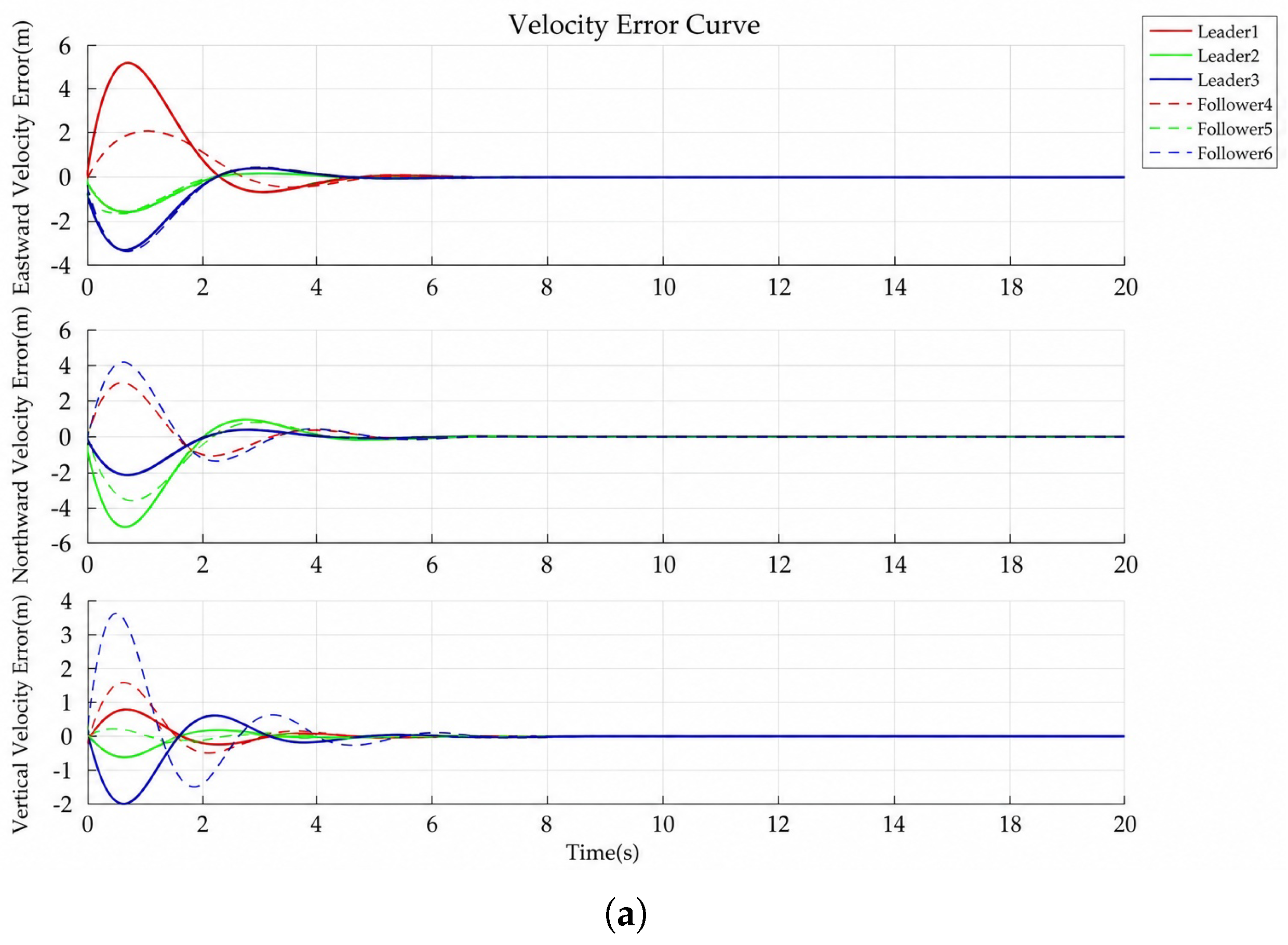
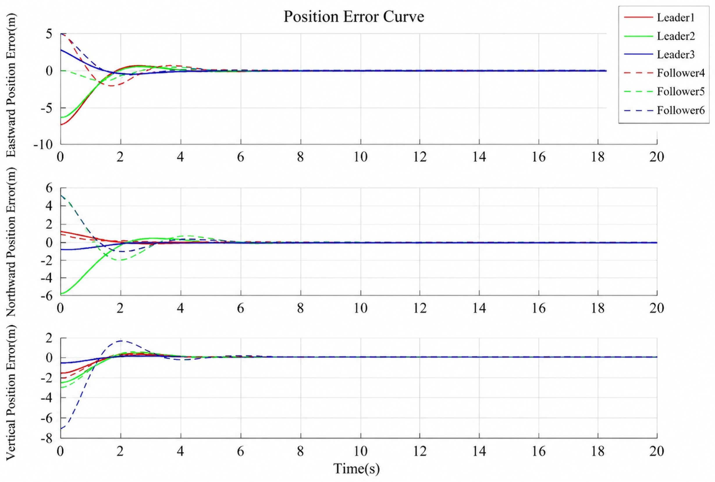
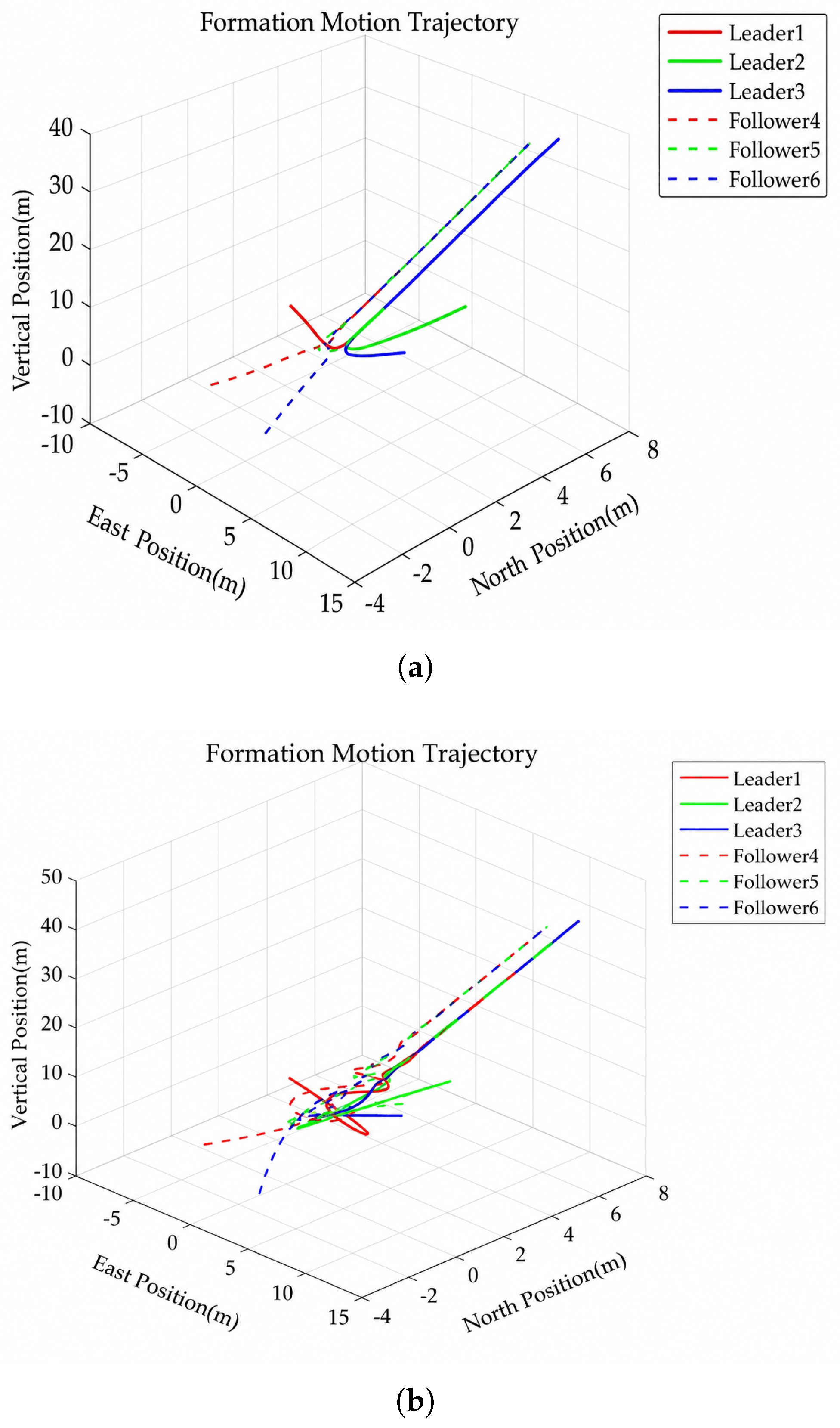
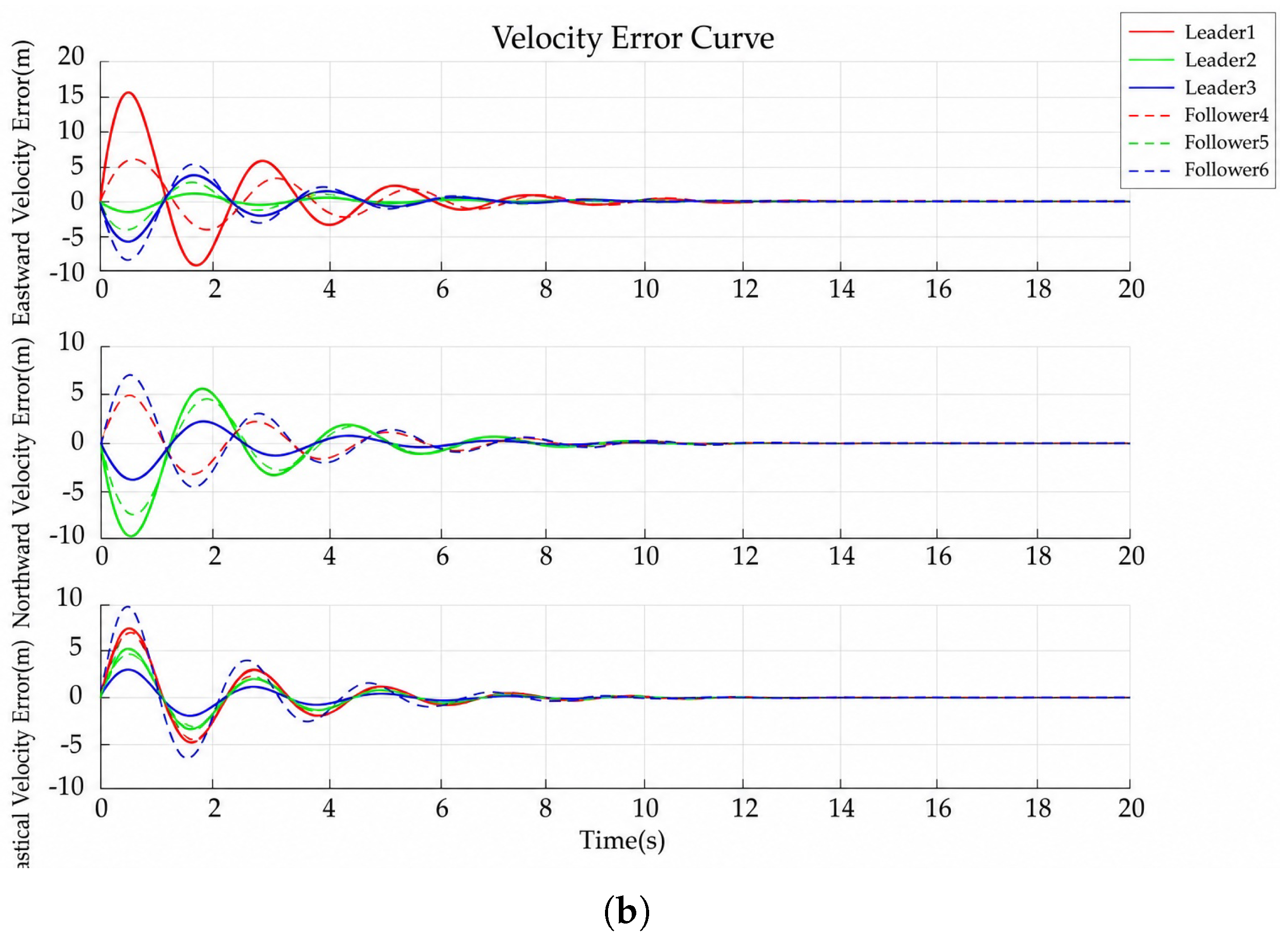
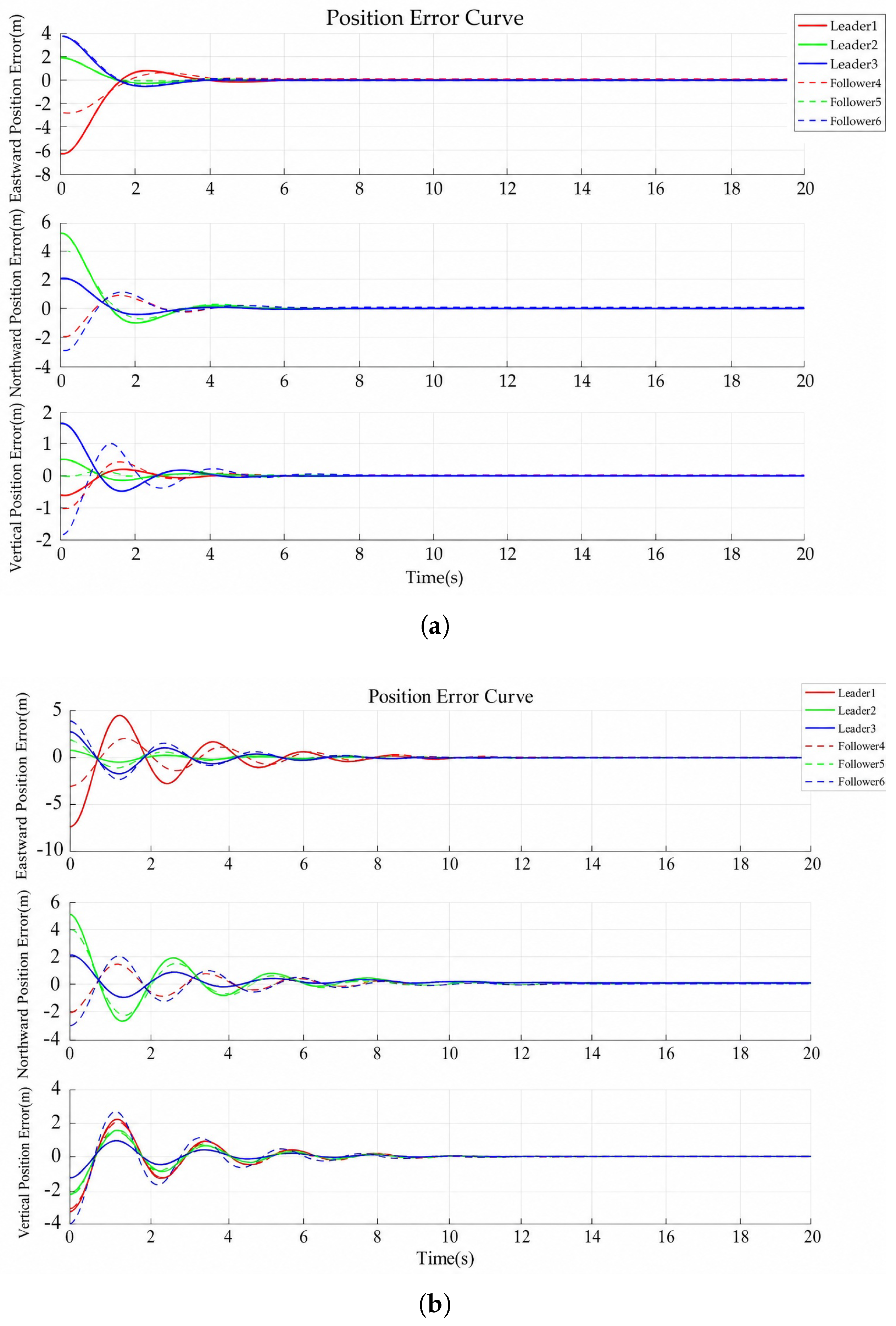
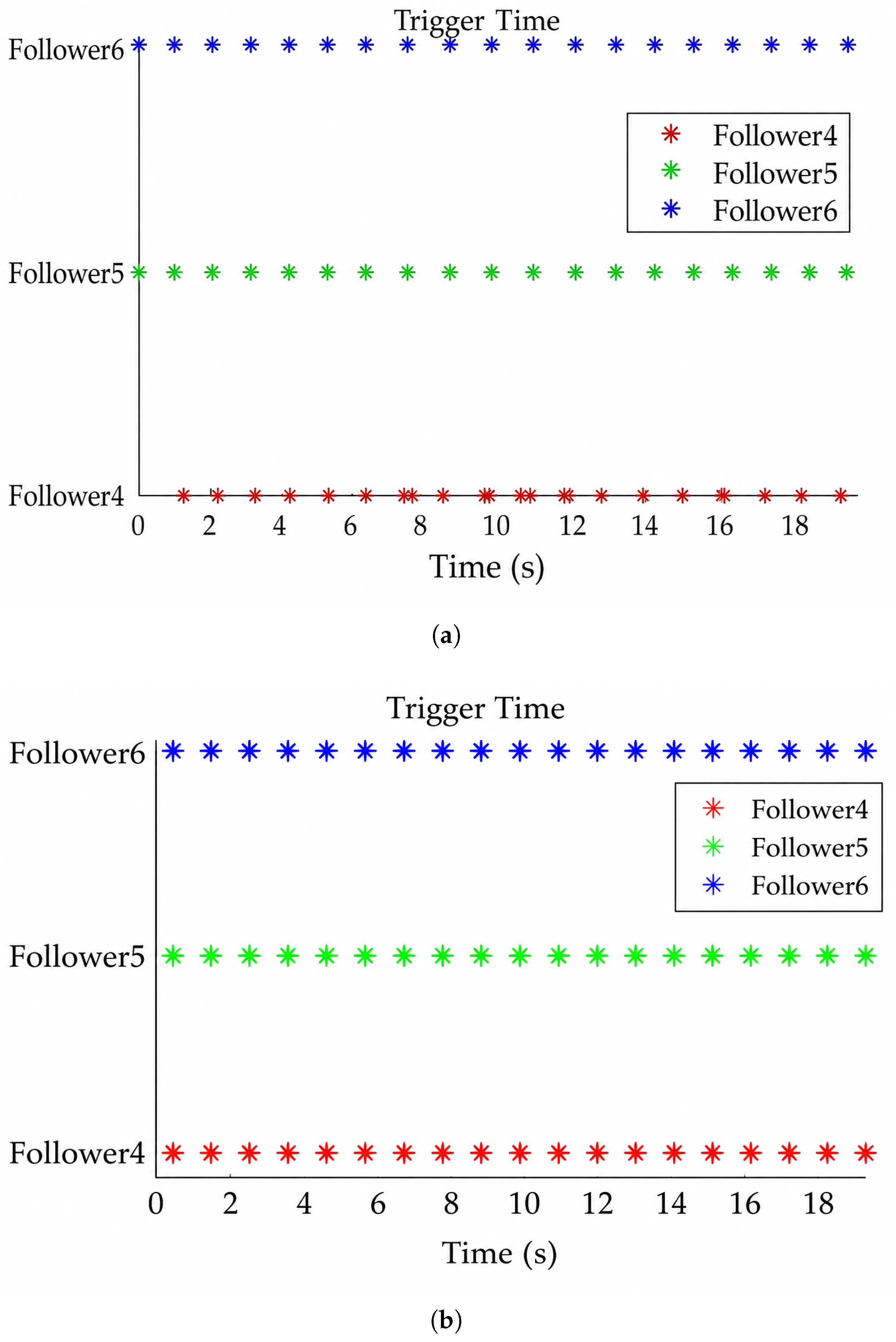
Simulate the system with the above parameters according to the method proposed in this paper and the comparative algorithms. The state and trigger time of the UAV cluster is recorded at each moment, and the formation motion of the UAVs from 0 to 20 s is illustrated. The solid line in the figure represents three leader drones, and the dotted line represents three follower drones. Figure 2 is the formation trajectory diagram of a UAV swarm in three-dimensional space. Figure 3 is the velocity error curve of the UAV formation in the east, north, and vertical directions. Figure 4 is the position error curve of the UAV formation in the east, north, and vertical directions. Figure 5 is the dynamic trigger time diagram of the UAV within 20 s.

Figure 2. Formation motion trajectory. (a) algorithm in this paper; (b) comparison algorithm.

Figure 3. Velocity error curve. (a) algorithm in this paper; (b) comparison algorithm.

Figure 4. Position error curve. (a) algorithm in this paper; (b) comparison algorithm.

Figure 5. Dynamic trigger time. (a) algorithm in this paper; (b) comparison algorithm.

Figure 2a shows that the UAV under the algorithm in this paper flies according to the predetermined trajectory, and the trajectory line is smooth. In Figure 2b, although the UAV of the comparison algorithm flies according to the predetermined trajectory, the trajectory line is more cluttered.

Figure 3a shows that the eastward velocity error of the UAV under the algorithm in this paper tends to 0 at 5 s; the error of the north speed tends to 0 at 5 s; the error of vertical velocity tends to 0 at 6 s. Figure 3b shows that the eastward velocity error of the comparison algorithm tends to zero at 11 s; the north speed error tends to zero at 10 s; the vertical velocity error tends to 0 at 10 s.

Figure 4a shows that the east position error and north position error of the algorithm in this paper tend to be 0 at 4 s, and the vertical position error tends to be 0 at 6 s. Figure 4b shows that the east position error of the comparison algorithm tends to be 0 at 11 s, the north position error tends to be 0 at 12 s, and the vertical position error tends to 0 at 10 s.

In this algorithm, as shown in Table 3, follower 4 triggers 28 times in 20 s; follower 5 triggers 47 times in 20 s; follower 6 triggers 59 times in 20 s. In comparison algorithm, follower 4 triggers 122 times in 20 s; follower 5 triggers 143 times in 20 s; follower 6 triggers 178 times in 20 s. The above results show that the dynamic event-triggered strategy proposed in this paper can not only achieve better control performance than the method proposed by Du et al. [23], but also save communication resources more effectively.

Table 3. Quantitative comparison of the proposed method and Du et al. [23].

Metric	Proposed	Du et al. [23]
Convergence time (position)	5 s	12 s
Convergence time (velocity)	6 s	11 s
Trigger count (Follower 4)	28	122
Trigger count (Follower 5)	47	143
Trigger count (Follower 6)	59	178

The formation trajectory of the method proposed by Du et al. [23] fluctuates greatly, and the trajectory line is more irregular. The method in this paper achieves a stable state at the 6th second, while the comparison method achieves formation control at the 12th second. Moreover, the number of triggers in this paper is much smaller than that of the comparison method. Therefore, the method in this paper can make UAV formation control quicker and more stable.

It should be noted that the method proposed by Du et al. [23] was not originally designed to handle communication delays. Therefore, the comparison primarily aims to demonstrate the advantages of incorporating delay compensation and dynamic event-triggering in formation control. The proposed method achieves faster convergence (6 s vs. 12 s) and significantly fewer trigger events, which validates the effectiveness of the delay compensation term and the dynamic event-triggering mechanism.

However, the proposed method also has certain limitations: (1) the current delay model assumes a constant delay $\tau \left(t\right)=0.1$ s, whereas in practice, communication delays are typically time-varying; (2) the parameter selection for the triggering mechanism requires solving LMIs, which may become computationally intensive for large-scale systems; and (3) the current framework assumes that the communication topology remains fixed, which may not hold in highly dynamic scenarios.

It is evident that the method in this paper has significant advantages compared to the comparison method; thus, simulation 2 no longer designs comparative experiments.

• Simulation 2:

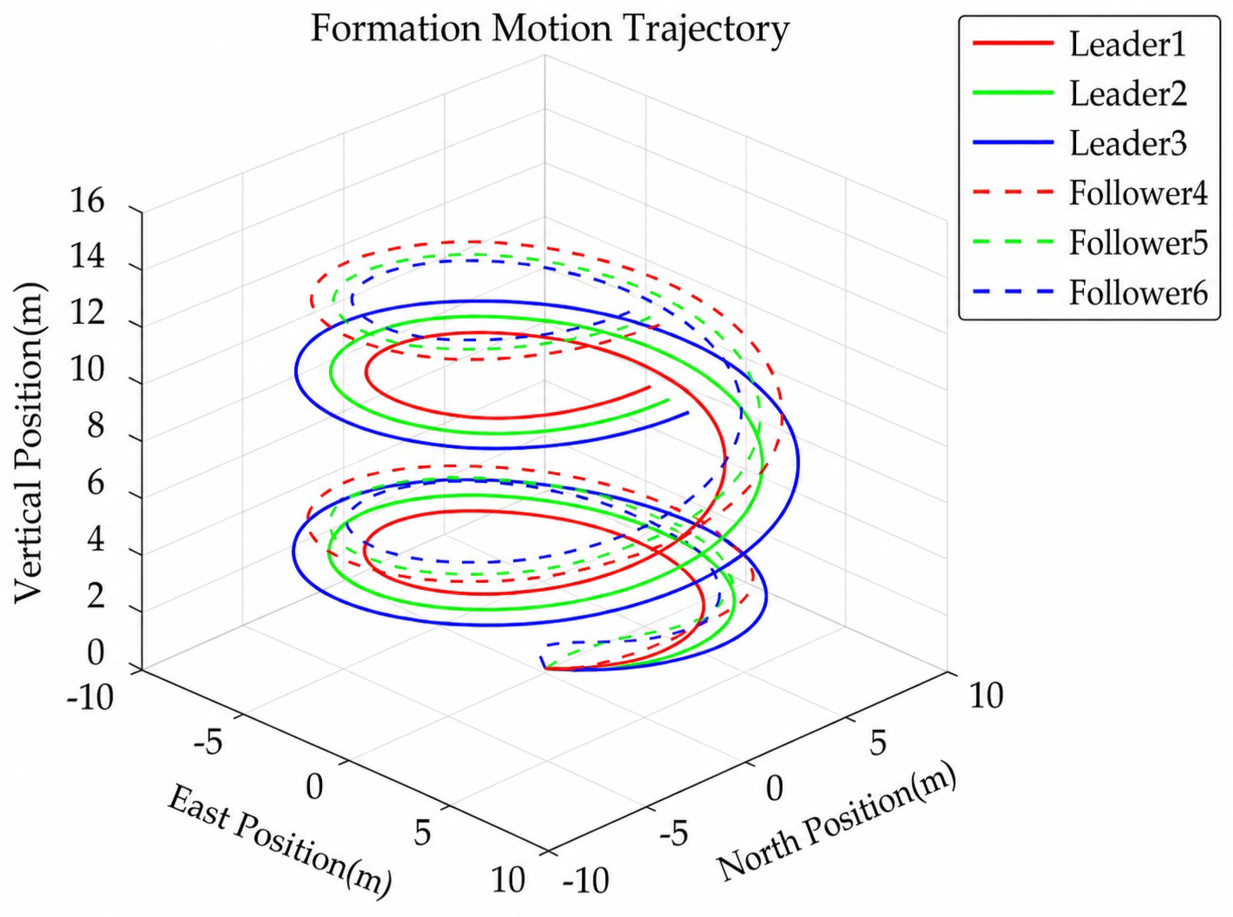
To further verify the stability of the system in this paper, the expected formation is set as a spiral formation. The leaders are designed to have different spiral radii. The spiral radius of Leader 1 is 5, the spiral radius of Leader 2 is 6, and the spiral radius of Leader 3 is 7. The spiral angular velocity is set to 0.5 radians per second, and the spiral forward speed is designed to be 0.5 m per second.

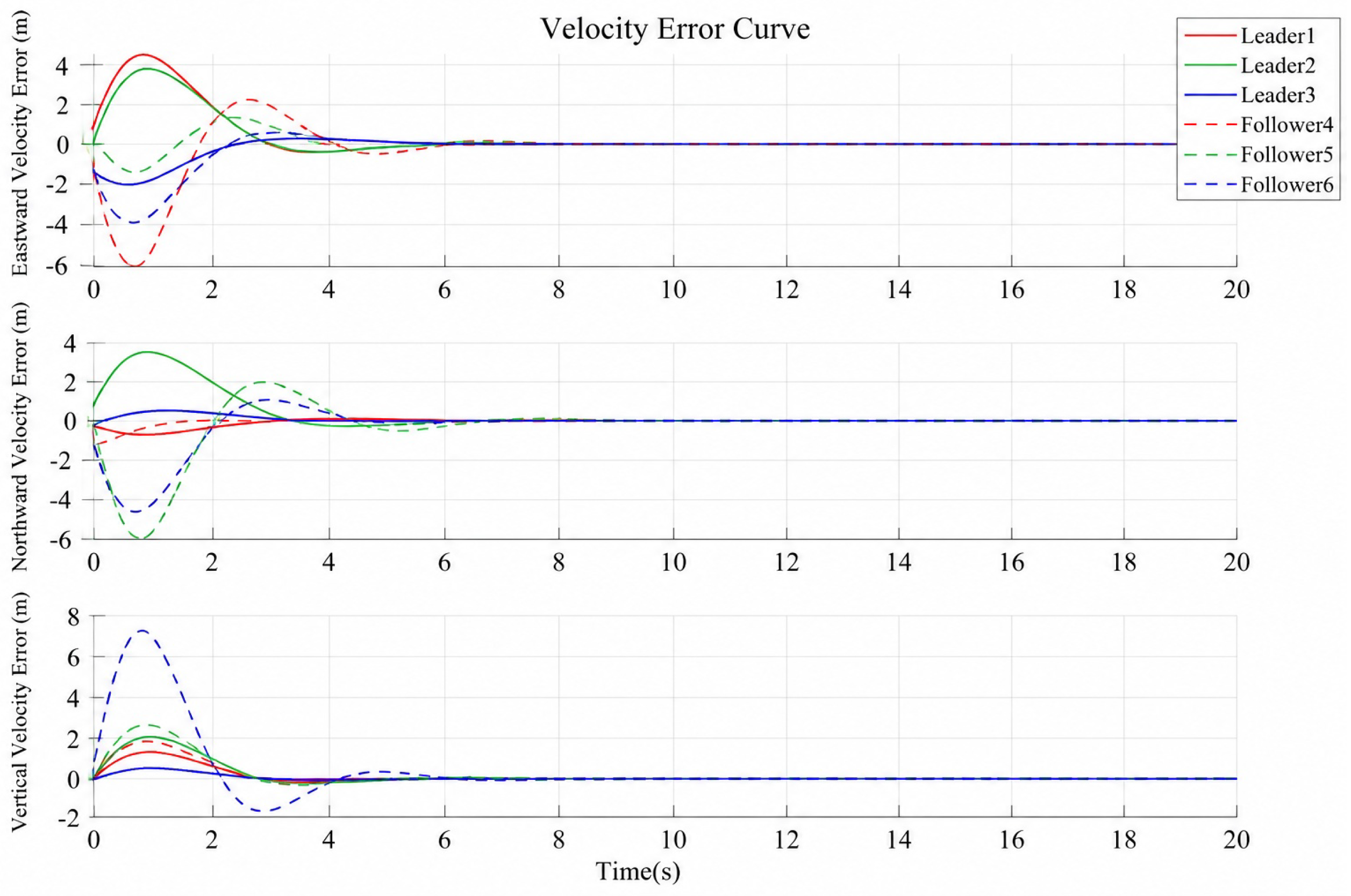
Figure 6 shows that the UAV flies along the predetermined spiral trajectory, and the trajectory line is well-defined. It can be seen from Figure 7 that the eastward velocity error fluctuates significantly between 0 and 4 s, eventually approaching 0 at 6 s. The maximum error is −6.5. The north velocity error tends to be 0 at 6 s, with a maximum error of −6. The vertical velocity error fluctuates significantly between 0 and 4 s, approaches zero at 6 s, and reaches a maximum error of 7. It can be observed from Figure 8 that the east position error and the vertical position error approach zero at 5 s, while the north position error approaches zero at 6 s. Combined with Figure 6, Figure 7 and Figure 8, it is evident that the formation of the UAV was established at 6 s, with both the speed and position error curves approaching zero. The desired formation state has been achieved, and the system has reached a stable state.

Figure 6. Formation motion trajectory (method described in this paper).

Figure 7. Velocity error curve (method described in this paper).

Figure 8. Position error curve (method described in this paper).

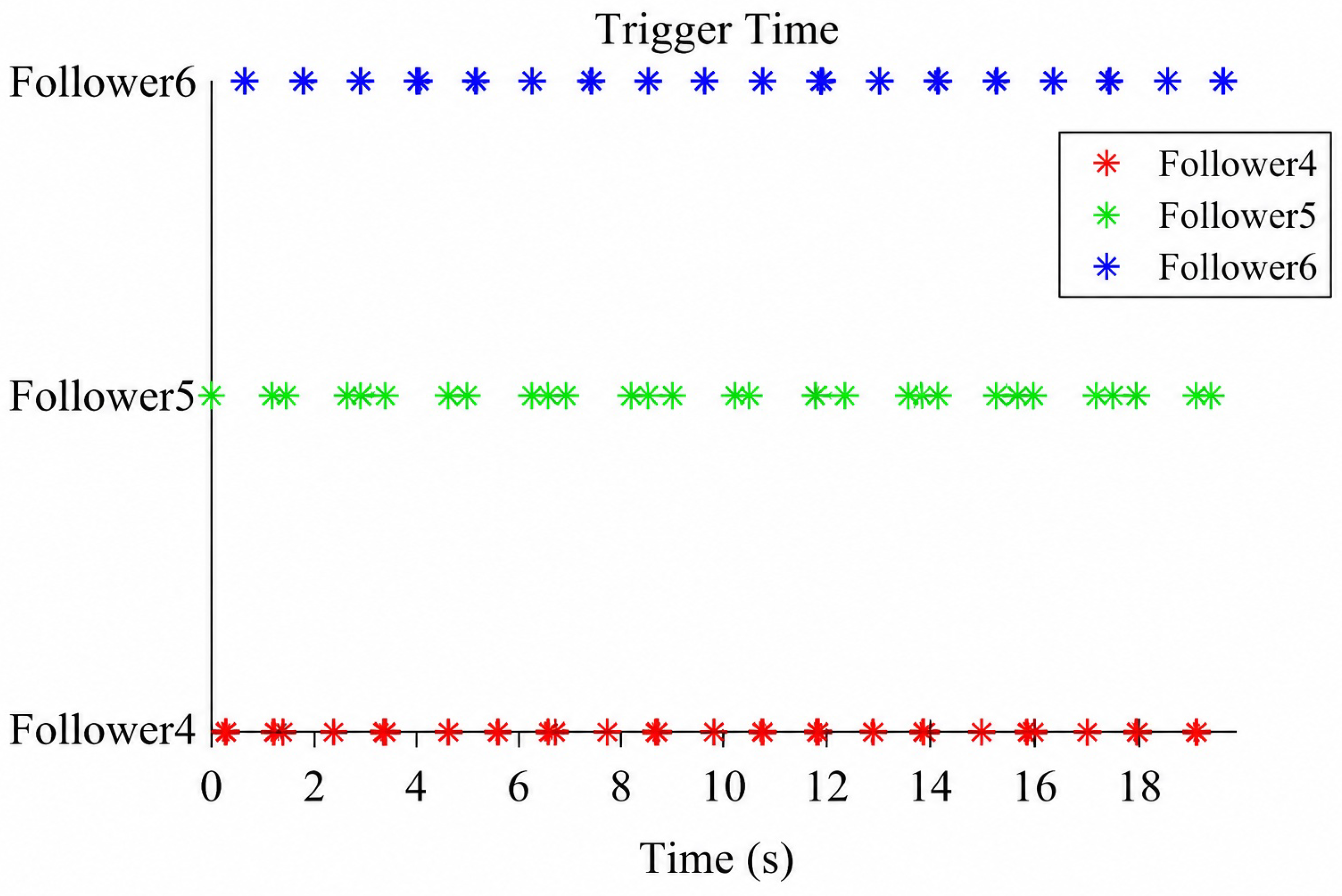
It can be seen from Figure 9 that follower 4 triggers 43 times within 20 s. Follower 5 triggers 45 times within 20 s. Follower 6 triggers 58 times within 20 s. It is proved that there is no Zeno behavior.

Figure 9. Dynamic trigger time.

• Simulation 3:

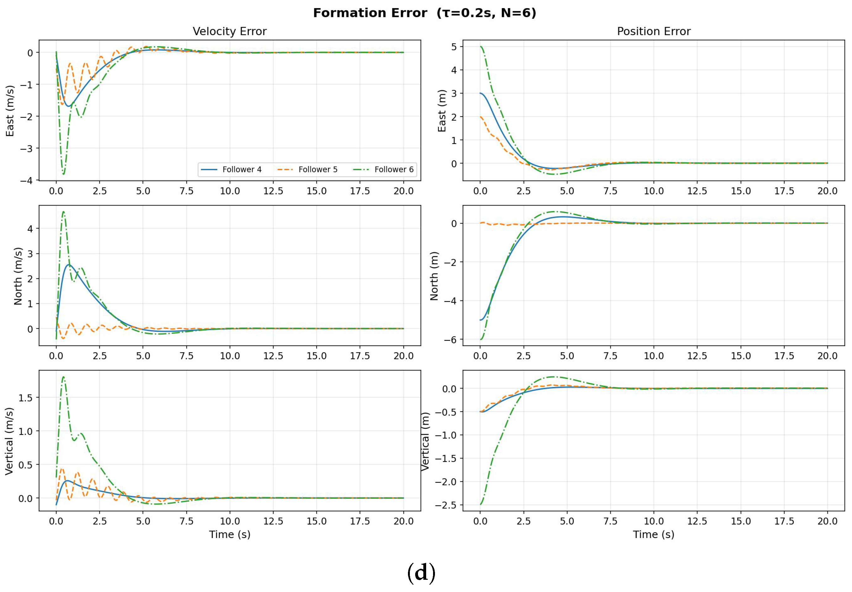
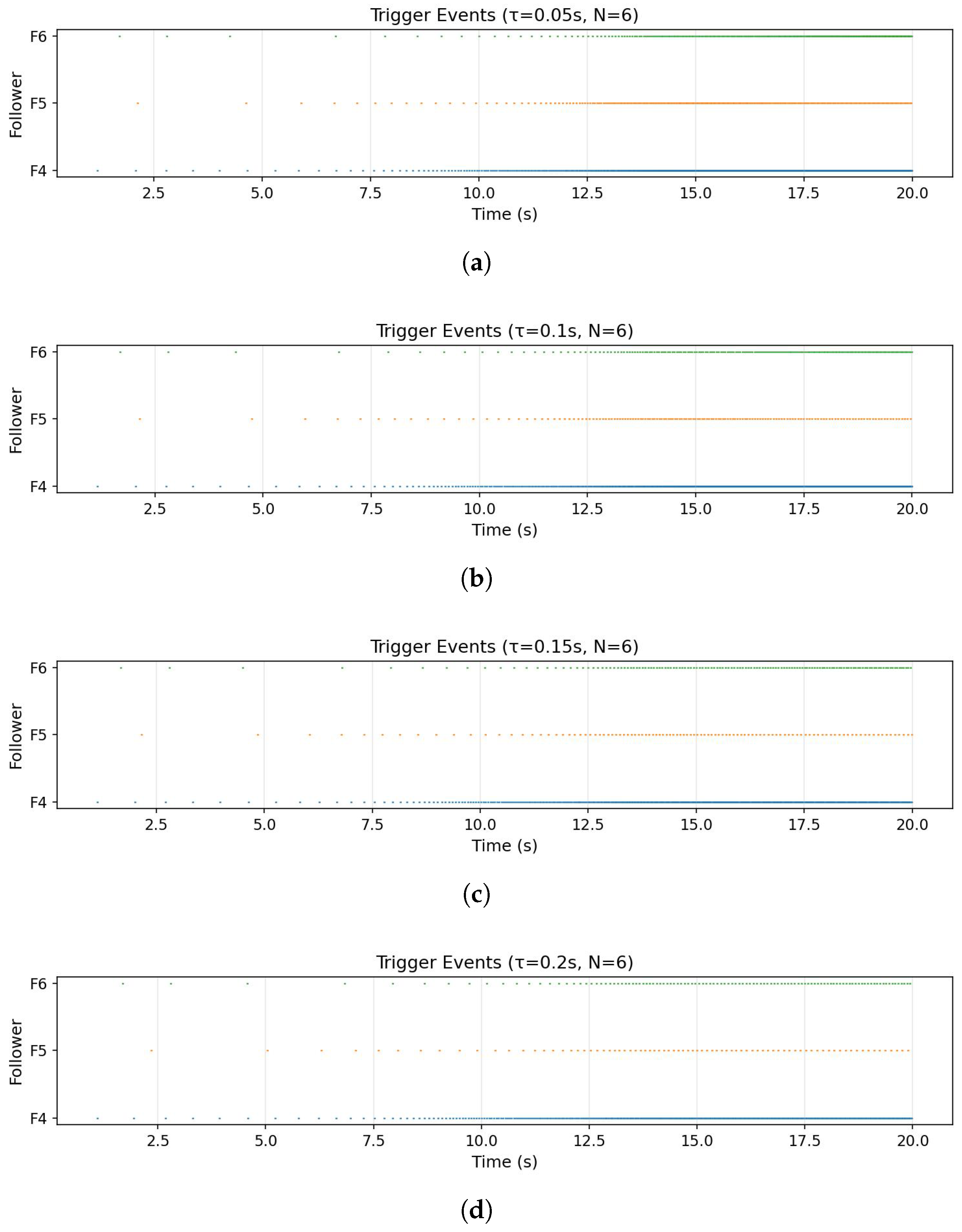
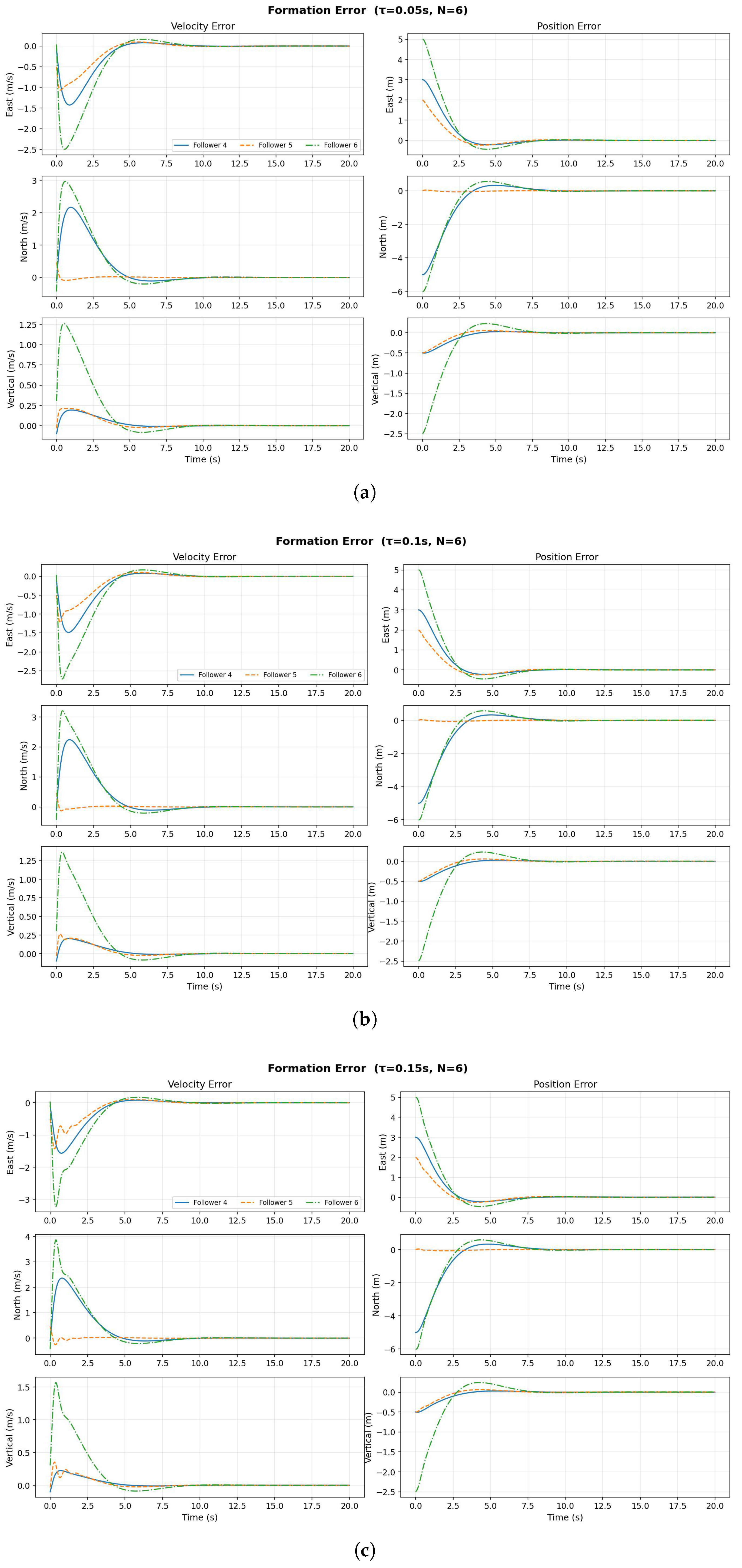
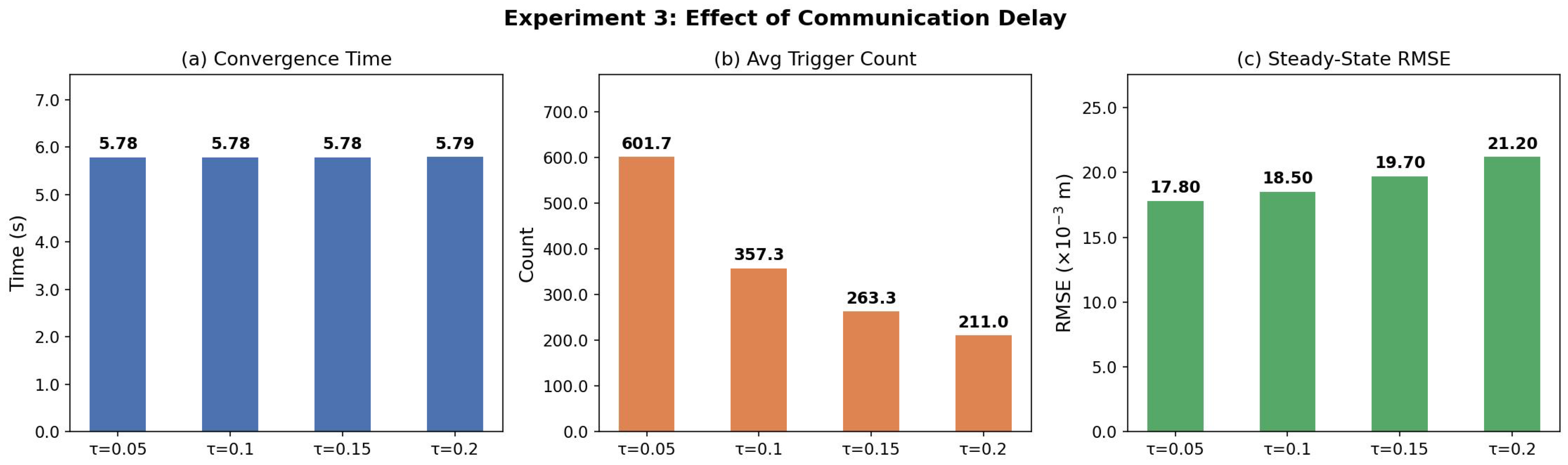
To evaluate the robustness of the proposed method under different communication delay conditions, four delay values are tested: $\tau =0.05$ s, $\tau =0.1$ s, $\tau =0.15$ s, and $\tau =0.2$ s. All other parameters remain consistent with Simulation 1. The convergence time, average trigger count, and steady-state performance are recorded for each delay condition.

As shown in Figure 10, Figure 11, Figure 12, and Table 4, the proposed method maintains stable formation control across all tested delay values. The position convergence time remains approximately 5.78 s for all delay conditions, demonstrating the robustness of the delay compensation mechanism. As the delay increases from 0.05 s to 0.2 s, the RMSE of position increases from 0.0178 m to 0.0212 m, while the average trigger count decreases from 601.7 to 211.0 due to the larger inter-event intervals. The maximum position error remains at 8.20 m across all cases, while the maximum velocity error increases from 4.07 m/s ($\tau =0.05$ s) to 6.30 m/s ($\tau =0.2$ s). These results demonstrate that the delay compensation term in the extended state observer effectively mitigates the impact of communication delays, and the system remains stable even under relatively large delays.

Figure 10. Position and velocity error curves under different communication delays. (a) $\tau =0.05$ s. (b) $\tau =0.1$ s. (c) $\tau =0.15$ s. (d) $\tau =0.2$ s.

Figure 11. Dynamic trigger time under different communication delays. (a) $\tau =0.05$ s. (b) $\tau =0.1$ s. (c) $\tau =0.15$ s. (d) $\tau =0.2$ s.

Figure 12. Comparison of performance metrics under different communication delays.

Table 4. Performance under different communication delays.

τ (s)	Conv. Time Pos. (s)	Conv. Time Vel. (s)	RMSE Pos. (m)	RMSE Vel. (m/s)	Avg. Triggers
0.05	5.78	3.63	0.0178	0.0092	601.7
0.10	5.78	3.59	0.0185	0.0098	357.3
0.15	5.78	3.55	0.0197	0.0104	263.3
0.20	5.79	3.52	0.0212	0.0113	211.0

• Simulation 4:

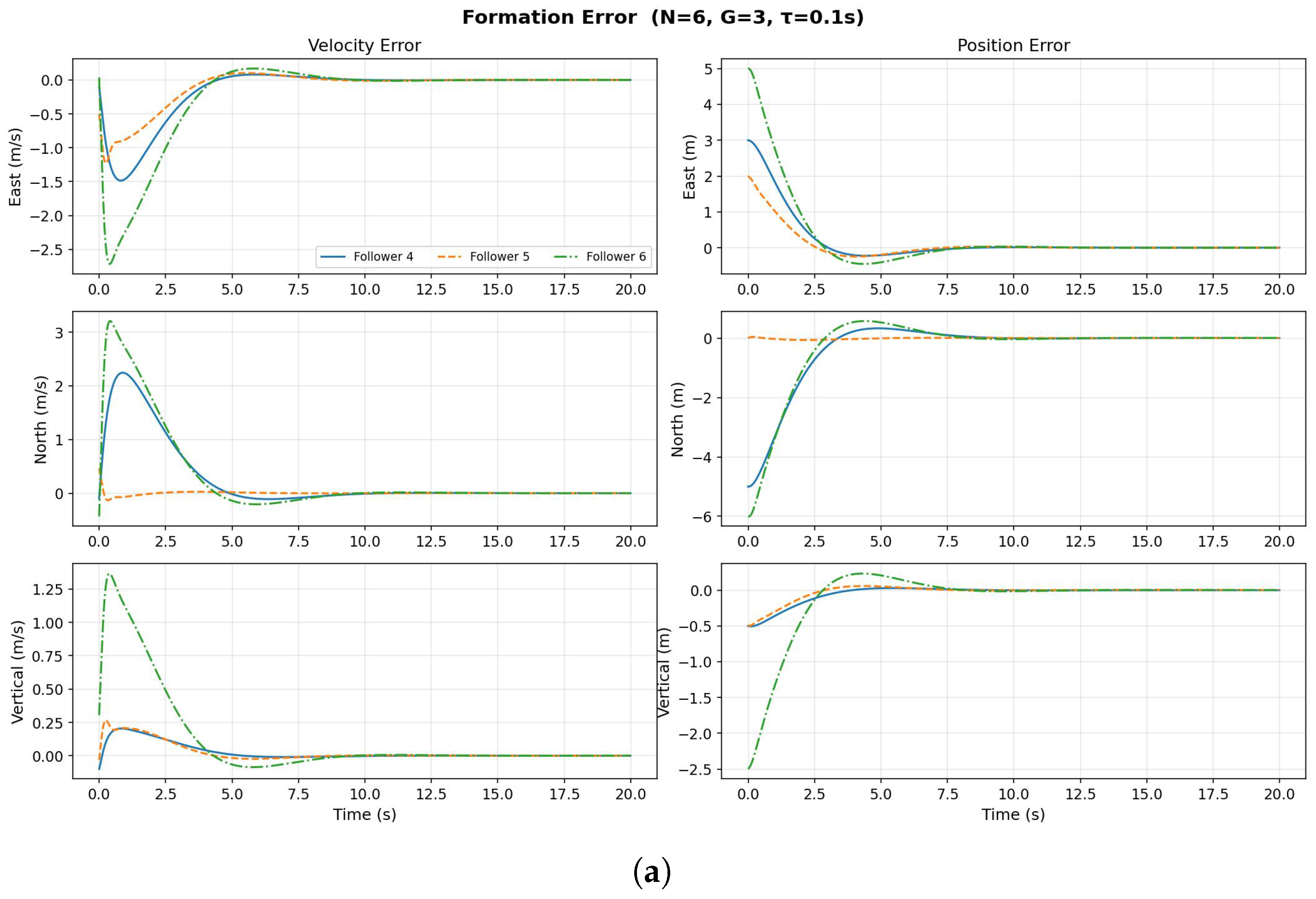
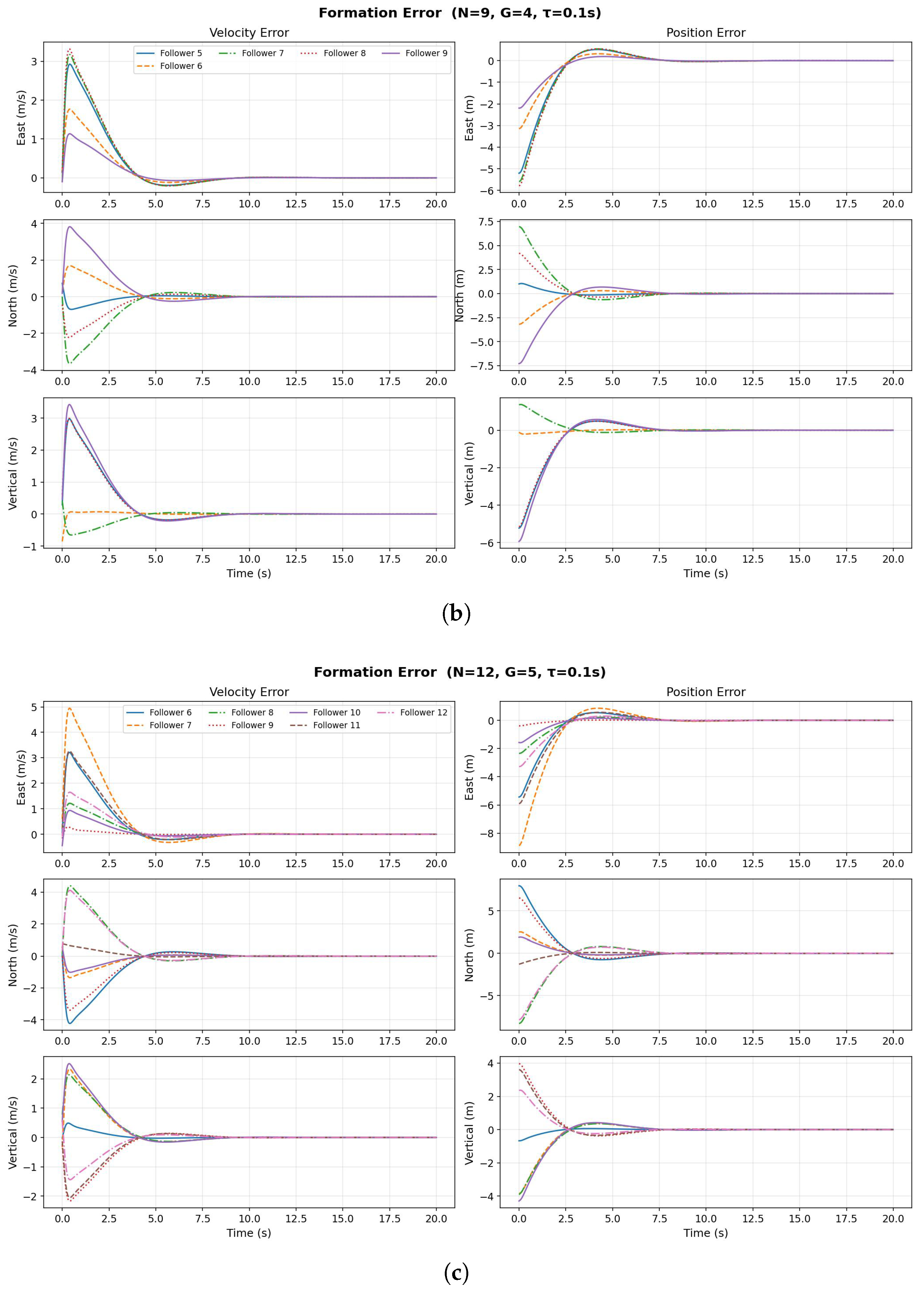
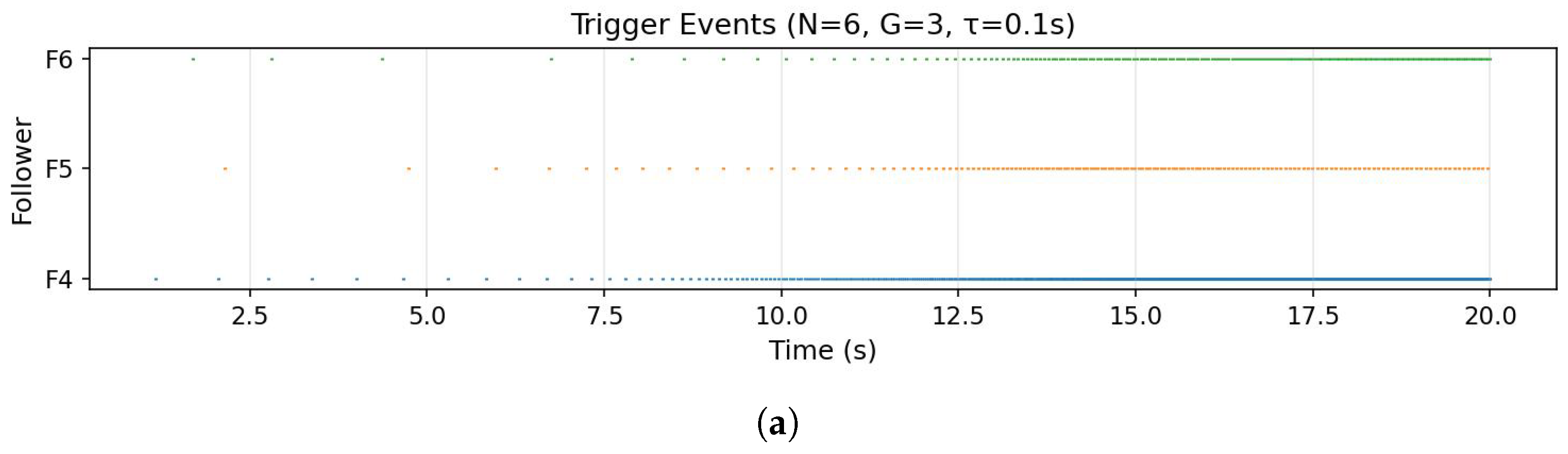
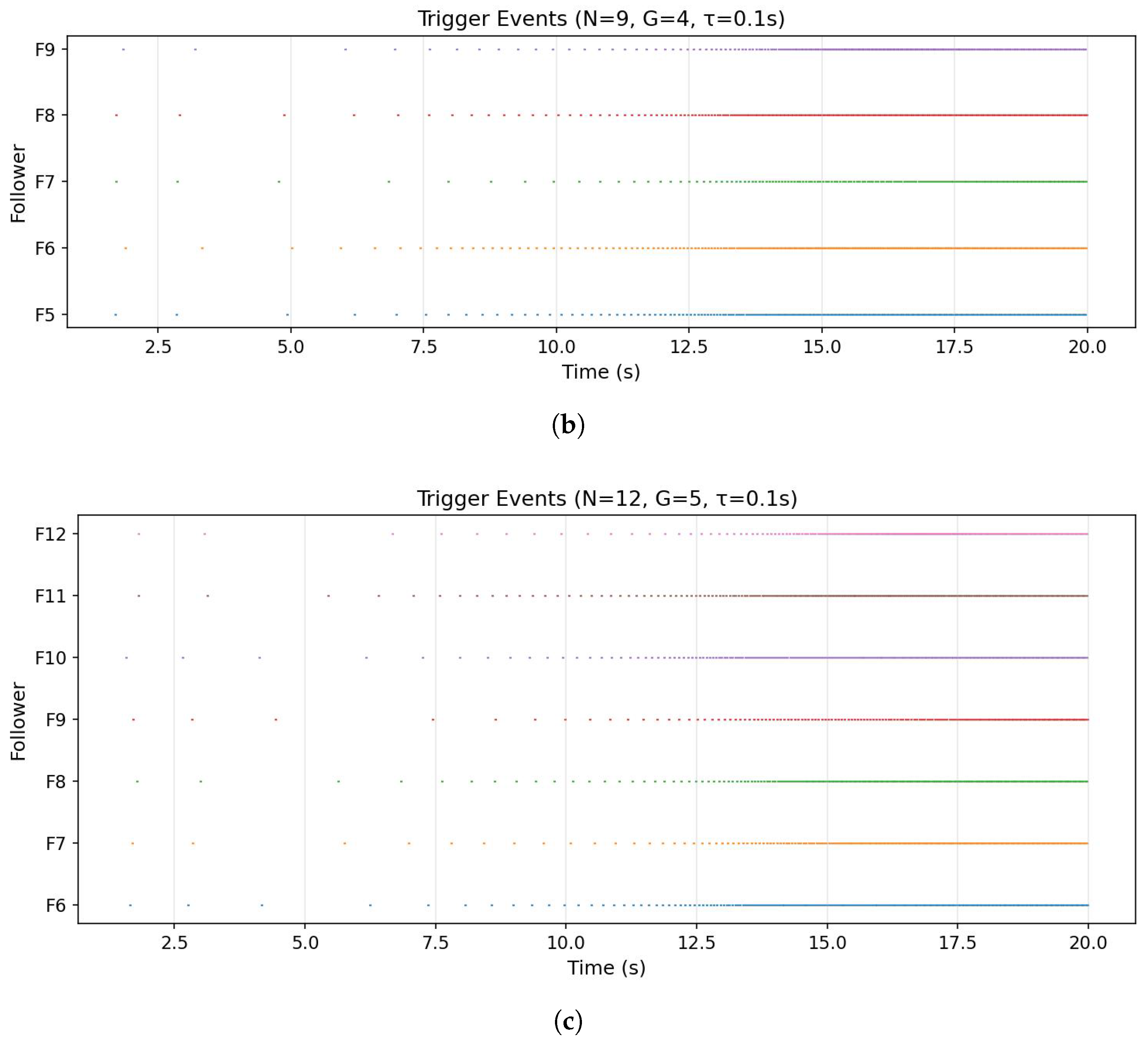
To verify the scalability of the proposed method, three different swarm sizes are tested: $N=6$ (3 leaders, 3 followers), $N=9$ (4 leaders, 5 followers), and $N=12$ (5 leaders, 7 followers). The communication delay is fixed at $\tau =0.1$ s for all cases.

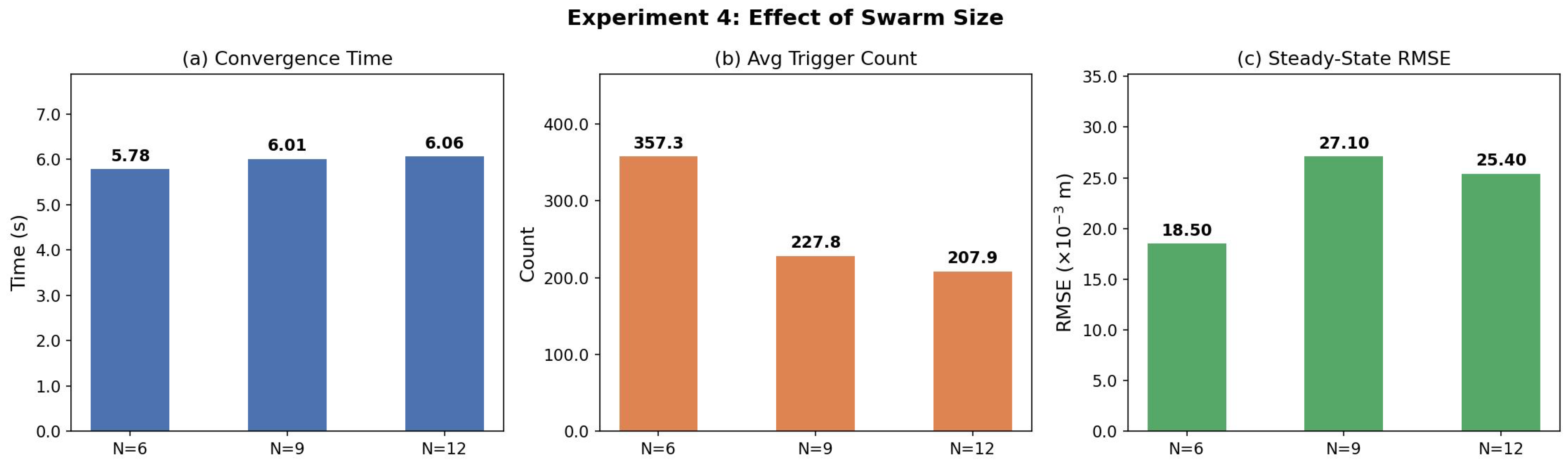
As shown in Figure 13, Figure 14, Figure 15, and Table 5, the proposed method successfully achieves formation control for all three swarm sizes. When the number of UAVs increases from 6 to 12, the position convergence time increases moderately from 5.78 s to 6.06 s, and the velocity convergence time increases from 3.59 s to 3.66 s. The RMSE of position increases from 0.0185 m to 0.0254 m, remaining at a very low level. The average trigger count per follower decreases from 357.3 to 207.9 as the swarm size grows, indicating improved communication efficiency in larger networks. These results confirm that the proposed method exhibits good scalability and can be applied to larger UAV swarms without significant performance degradation.

Figure 13. Position and velocity error curves under different swarm sizes. (a) $N=6$. (b) $N=9$. (c) $N=12$.

Figure 14. Dynamic trigger time under different swarm sizes. (a) $N=6$. (b) $N=9$. (c) $N=12$.

Figure 15. Comparison of performance metrics under different swarm sizes.

Table 5. Scalability analysis with different swarm sizes.

N	Leaders	Followers	Conv. Time Pos. (s)	Conv. Time Vel. (s)	RMSE Pos. (m)	Avg. Triggers
6	3	3	5.78	3.59	0.0185	357.3
9	4	5	6.01	3.65	0.0271	227.8
12	5	7	6.06	3.66	0.0254	207.9

6. Conclusions

This study investigates the formation control problem of multi-UAV systems with multiple leaders in the case of communication delay and waste of communication resources. To address this problem, a state observer and a controller are designed so that the UAVs in the system can follow the leaders to form the desired formation. The following conclusions are drawn:

(1)

The dynamic event triggering mechanism proposed in this paper can adjust the triggering time in real time according to the state of the UAV system, thereby avoiding unnecessary data transmission. Compared with the traditional periodic communication method or other existing methods, this mechanism significantly reduces the communication frequency and avoids the waste of communication resources.

(2)

The combination of a multi-leader architecture and dynamic event-triggered mechanism improves the reliability and resource utilization efficiency of multi-UAV systems. The multi-leader architecture ensures that the system can maintain basic operations and formation stability when the leader fails or communication is interrupted, while the dynamic event-triggered mechanism reduces unnecessary communication and computing burdens, makes the system more efficient and reliable, and enhances the system’s adaptability and robustness in complex environments.

(3)

The state observer designed in this paper can effectively estimate the actual state of the UAV, including critical information such as its position and velocity. Even in the presence of communication delays, the state change can be accurately predicted by the time delay compensation term, thereby providing precise state feedback for the controller.

References

1. Hu, S.C.; Chang, Z.L.; He, Q.W. Research on intelligent route planning of low-altitude UAV surveying and mapping based on ground features and landforms. Geogr. Space Inf. 2025, 23, 65–68. [Google Scholar]
2. Zeng, Z.Y.; Peng, W.S.; Li, Y.K. Connotation, development and challenges of reliability technology of intelligent UAV swarm. Acta Armamentarii 2025, 46, 3–20. [Google Scholar]
3. Yang, G.Q.; Xu, H.Q.; Mao, T.L. Evaluation of border reconnaissance and patrol capability of quadrotor UAV based on extension theory. Ordnance Ind. Autom. 2024, 43, 93–96. [Google Scholar]
4. Chen, C.L.; Zheng, Z.X.; Xu, T.Y. YOLO-based UAV technology: A review of the research and its applications. Drones 2023, 7, 190. [Google Scholar] [CrossRef] [Scilit]
5. Javaid, S.; Saeed, N.; Qadi, Z. Communication and control in collaborative UAVs: Recent advances and future trends. IEEE Trans. Intell. Transp. Syst. 2023, 24, 5719–5739. [Google Scholar] [CrossRef] [Scilit]
6. Xu, H.; Liu, P.Z.; Chen, X.Y. D2SLAM: Decentralized and distributed collaborative visual-inertial SLAM system for aerial swarm. IEEE Trans. Robot. 2024, 40, 3445–3464. [Google Scholar]
7. Wang, Y.T.; Su, Z.; Xu, Q.C. A secure and intelligent data sharing scheme for UAV-assisted disaster rescue. IEEE/ACM Trans. Netw. 2023, 31, 2422–2438. [Google Scholar] [CrossRef] [Scilit]
8. Zhou, B.Y.; Xu, H.; Shen, S.J. Racer: Rapid collaborative exploration with a decentralized multi-UAV system. IEEE Trans. Robot. 2023, 39, 1816–1835. [Google Scholar] [CrossRef] [Scilit]
9. Wu, Y.L.; Sun, C.S. Development and operational application of compact Photoelectric pod for military UAV. Laser Infrared 2023, 53, 1568–1574. [Google Scholar]
10. Ge, Y.; Liao, Y.L.; Wang, B. A survey of multi-agent formation control based on null space behavior fusion. J. Harbin Eng. Univ. 2024, 45, 1442–1450. [Google Scholar]
11. Guo, J.D.; Liu, Z.G.; Song, Y.G. Research on Multi-UAV Formation and Semi-Physical Simulation with Virtual Structure. IEEE Access 2023, 11, 126027–126039. [Google Scholar]
12. Zhao, Y.; Gao, K.; Huang, P.F. Specified time affine formation maneuver control of multiagent systems over directed networks. IEEE Trans. Autom. Control 2024, 69, 1936–1943. [Google Scholar]
13. Liu, Y.; Chen, C.; Wang, Y. A fast formation obstacle avoidance algorithm for clustered UAVs based on artificial potential field. Aerosp. Sci. Technol. 2024, 147, 108974. [Google Scholar] [CrossRef] [Scilit]
14. Li, H. Research on Cooperative Formation Control and Obstacle Avoidance of Quadrotor UAV under Leader-Follower Structure. Master's Thesis, Beijing University of Chemical Technology, Beijing, China, 2022. [Google Scholar] [PubMed]
15. Shi, H.T.; Wang, M.; Wang, C. Leader-follower formation learning control of discrete-time nonlinear multiagent systems. IEEE Trans. Cybern. 2023, 53, 1184–1194. [Google Scholar] [PubMed]
16. Zhang, X.H.; Li, Q.Q.; Li, Y.K. Distributed cooperative control of leader-follower multi-agent systems. J. Henan Inst. Technol. 2025, 33, 18–22. [Google Scholar]
17. Li, J.C.; Liu, J.M.; Huangfu, S.Q. Leader-follower formation of light-weight UAVs with novel active disturbance rejection control. Appl. Math. Model 2023, 117, 577–591. [Google Scholar]
18. Zou, N.; Shi, Y.K. Formation control method of quadrotor UAVs based distance consistency. Fire Control Command Control 2024, 49, 167–172+179. [Google Scholar]
19. Xue, Y.H.; Luo, Y.J.; Zhu, M. UAV formation control method based on consistency strategy. Proc. IOP Conf. Ser. Earth Environ. Sci. 2020, 440, 052084. [Google Scholar] [CrossRef] [Scilit]
20. Liu, J.; Zhang, Y.L.; Yu, Y. Fixed-time leader-follower consensus of networked nonlinear systems via event/self-triggered control. IEEE Trans. Neural Netw. Learn. Syst. 2020, 31, 5029–5037. [Google Scholar] [PubMed]
21. Ni, J.K.; Shi, P.; Zhao, Y. Fixed-time event-triggered output consensus tracking of high-order multiagent systems under directed interaction graphs. IEEE Trans. Cybern. 2022, 52, 6391–6405. [Google Scholar]
22. Liu, R.Y.; Qu, B.Y.; Wei, T. Research on UAV formation obstacle avoidance based on consistency control. In Proceedings of the 2023 IEEE 12th Data Driven Control and Learning Systems Conference (DDCLS), Xiangtan, China, 12–14 May 2023; IEEE: Piscataway, NJ, USA, 2023; pp. 155–160. [Google Scholar]
23. Du, C.K.; Liu, X.D.; Liu, H.K. Distributed event-triggered consensus control for general linear multi-agent systems under-directed graph. In Proceedings of the IEEE 56th Annual Conference on Decision and Control, Melbourne, Australia, 12–15 December 2017; IEEE: Piscataway, NJ, USA, 2017; pp. 4550–4555. [Google Scholar]
24. Yang, Z.Q.; Xia, C.Q.; Liu, Y.Q. A dynamic event triggering formation method for multi-agent systems under communication delay constraints. Control Eng. China 2025, 32, 126–134. [Google Scholar]
25. Yu, W.W.; Chen, G.R.; Cao, M. Some necessary and sufficient conditions for second-order consensus in multi-agent dynamical systems. Automatica 2010, 46, 1089–1095. [Google Scholar]
26. Tang, Z.J.; Huang, T.Z.; Shao, J.L. Consensus of second-order multi-agent systems with nonuniform time-varying delays. Neurocomputing 2012, 97, 410–414. [Google Scholar]
27. Li, H.J.; Zhu, Y.L.; Wang, J.T. Consensus of nonlinear second-order multi-agent systems with mixed time-delays and intermittent communications. Neurocomputing 2017, 251, 115–126. [Google Scholar]
28. Hou, W.Y.; Fu, M.Y.; Zhang, H.; Wu, Z. Consensus conditions for general second-order multi-agent systems with communication delay. Automatica 2017, 75, 293–298. [Google Scholar]
29. Huang, Y.; Li, Y.G.; Hu, W.F. Distributed rotating formation control of second-order leader-following multi-agent systems with nonuniform delays. J. Frankl. Inst. 2019, 356, 3090–3101. [Google Scholar]
30. Zhang, Z.H.; Peng, S.G. Research on leader-follower consensus of multi-agent systems with time delays. Appl. Res. Comput. 2019, 36, 1333–1337. [Google Scholar]
31. Ma, Z.W.; Qi, J.T.; Wang, M.M. Time-Varying Formation Tracking Control for Multi-UAV Systems with Directed Graph and Communication Delays. In Proceedings of the 2021 40th Chinese Control Conference (CCC), Shanghai, China, 26–28 July 2021; IEEE: Piscataway, NJ, USA, 2021; pp. 5436–5441. [Google Scholar]
32. Du, S.L.; Liu, T.; Ho, D.W. Dynamic event-triggered control for leader-following consensus of multiagent systems. IEEE Trans. Syst. Man. Cybern. Syst. 2018, 50, 3243–3251. [Google Scholar]
33. Wang, Z.Y.; Chadli, M.; Ding, S.X. A dynamic event-triggered approach for observer-based formation control of multi-agent systems with designable inter-event time. Syst. Control Lett. 2025, 195, 105970. [Google Scholar]
Disclaimer/Publisher’s Note: The statements, opinions and data contained in all publications are solely those of the individual author(s) and contributor(s) and not of MDPI and/or the editor(s). MDPI and/or the editor(s) disclaim responsibility for any injury to people or property resulting from any ideas, methods, instructions or products referred to in the content.
Article Metrics
Citations
Article Access Statistics
Multiple requests from the same IP address are counted as one view.