


Abstract
Air-jet looms are widely used for weaving lightweight fabrics due to their outstanding high performance. To enhance the overall structural strength of air-jet looms and reduce operational vibration, dynamic analysis and structural parameter optimization of the loom frame system were carried in this study. First, after the structural designing and finite element modeling, the modal tests of the loom frame system were conducted. The modal results showed the high consistency between the simulation and experiment, confirming the accuracy of the dynamic model. Then, the dynamic characteristics and maximum stress data of the frame were obtained and analyzed through vibration tests and simulation calculations. The results indicated that the maximum deformation occurred at the middle of the beam while the maximum stress occurred at the connection between the lower beam and the wall panel. Moreover, the loom frame parameter optimization model was constructed based on the BA-HHO-SVR (Balanced Adaptive—Harris Hawks Optimization—Support Vector Regression) algorithm, demonstrating excellent learning and predictive capabilities. Eventually, the optimal combination of the frame structural parameters was obtained through above optimization algorithm. Furthermore, the effectiveness and reliability of the optimal combination were verified by finite element calculations. The vibration analysis method and optimization strategy proposed in this study provide valuable guidance for subsequent structural design and optimization of the high-end textile equipment.
1. Introduction
As a foundational and pillar industry of the national economy, the textile sector is accelerating its global transformation toward high-speed, intelligent, and green manufacturing, imposing stringent demands on the performance of core equipment. Air-jet looms, renowned for their high weaving speeds and automation levels, dominate a significant share of the global shuttle-less loom market [1,2,3] and serve as core equipment for producing high-end fabrics. As the “skeleton” of air-jet looms, the frame’s stability directly impacts weaving precision and machine lifespan. However, prolonged exposure to high-frequency, complex loads often triggers vibrations and resonance, leading to malfunctions and quality issues, becoming a bottleneck for industry-wide quality improvement and efficiency gains [4,5].
During operation, traditional air-jet looms rely on the spindle system to drive coordinated functions such as weft insertion and weft drawing. As the machine’s supporting structure, the frame endures prolonged exposure to high-frequency alternating loads and airflow excitation [6]. This sustained dynamic loading readily induces frame vibrations and may even trigger structural resonance. This leads to surface defects in fabrics, component fatigue damage, and reduced overall operational stability, becoming a bottleneck that constrains both high-speed operation and the long-term reliability of the loom [7].
Against this backdrop, it is evident that the primary factor currently affecting production efficiency in air-jet looms is weaving speed [8]. The key factor behind the disparity in weaving speeds among different looms is the inadequate dynamic performance of the frame system. Severe overall frame vibration prevents stable operation at higher speeds. Therefore, conducting dynamic analysis and structural parameter optimization research on the air-jet loom frame system [9] holds significant practical importance for enhancing the core technological level of air-jet looms and promoting the high-quality development of the textile equipment industry.
To enhance the structural performance of looms, scholars worldwide have pursued structural optimization research from diverse perspectives [10]. Qiu developed a novel dual-shaft cam opening system by integrating mechanism analysis, theoretical calculations, modeling and simulation, and experimental validation. This innovation overcomes the spatial constraints and load-bearing limitations of traditional conjugate cam opening mechanisms. This effectively resolves contact wear issues between cams and rotors, facilitating design innovation and performance enhancement for conjugate cam opening mechanisms in high-speed looms [11]. Schwarzfischer, F., introduced the design and development of a suitable mechanism for driving head frames. Following the requirement specification, structural synthesis was performed. A novel head frame mechanism was designed for air-jet looms equipped with high-volume low-pressure (HVLP) relay nozzles [12]. Xi proposed an improved method for rapier looms, which reduces flexible deformation effects by increasing the cross-sectional dimensions and enhancing structural rigidity. The results showed that optimizing motion parameters reduced maximum belt acceleration by 35.7% and improved motion stability. Optimizing structural rigidity significantly decreased acceleration errors in the rapier belt and enhanced motion accuracy [13]. Eren Recep proposed a kinematic design method for rapier drive mechanisms that incorporates spatial mechanisms and analyzes rapier motion curves. The study revealed that the position of the oscillating link within the spatial mechanism and the main shaft angle during rapier entry into the shed have the most significant influence on the rapier motion curve. Gear ratios also affect the rapier motion curve. By modifying these parameters, different rapier motion curves can be obtained [14].
While these efforts have advanced specific subsystems, reviewing the current research landscape in weaving equipment [15], systematic studies on high-speed, high-frequency jet looms remain relatively scarce. Consequently, the vibration evolution patterns during high-efficiency operation remain poorly understood. Second, existing academic achievements are largely confined to kinematic or dynamic analyses of specific moving components such as the weft insertion mechanism [16] or the shedding mechanism [17], often neglecting the frame system itself, which serves as the “skeleton” of the entire machine. In reality, the frame system does more than merely provide structural support; it bears complex alternating mechanical stresses and random excitation forces. The quality of its dynamic characteristics directly determines the steady-state response and service life of the entire machine. Therefore, conducting dynamic modeling and structural optimization research on the frame system of air-jet looms is not only theoretically necessary to reveal the “mechanism–frame” coupled vibration mechanisms under complex weaving conditions but also key to achieving high-speed, precision, and long-term operational stability in air-jet looms, holding profound academic value and engineering significance [18].
Concurrently, at the parameter optimization methodology level, the integration of intelligent algorithms with surrogate models has emerged as an effective approach to enhancing structural performance [19]. Researchers globally have extensively employed techniques such as genetic algorithms and particle swarm optimization to achieve automated tuning of structural dimensions and profile thickness parameters, yielding significant improvements in weight reduction, stress mitigation, and natural frequency enhancement. Wang proposed a novel hybrid genetic-particle swarm algorithm (L-GPS) with enhanced local search capability for structural optimization problems. This algorithm integrates the global search capability of genetic algorithms, the local development capability of particle swarm optimization, the strong local search capability of finite memory quasi-Newton algorithms, and an optimal switching point evaluation strategy that self-adjusts for both global and local searches. L-GPS achieves faster convergence rates than widely known stochastic methods across a broad class of benchmark test functions [20]. Tsiptsis, Ioannis N., investigates structural optimization by analyzing two-dimensional lattice and frame towers using a PSO-based optimizer, integrating NURBS (Non-Uniform Rational B-Splines) into both the structural analysis solver and PSO (Particle Swarm Optimization). The research findings indicate that PSO methods can be flexibly applied to the structural optimization of both straight and curved towers [21]. Dos Santos, AT proposed a novel simplified approach combining genetic algorithms (GA) with the boundary element method (BEM), achieving smooth boundaries for structural shape optimization by applying simple polynomial fitting techniques. The results demonstrate significant improvements in structural performance and material reduction, indicating this method serves as an effective tool for structural shape optimization [22].
Despite these promising advancements, optimization data for jet loom frame structural improvements via parameter optimization remains insufficient, and the adaptability of existing algorithms to loom structural parameters remains unverified. Under complex operating conditions, the coupled action mechanism of multiple excitation loads on the frame remains incompletely understood [23], leading to poor alignment between optimization models and actual operating conditions. Concurrently, existing optimization algorithms exhibit limitations in efficiency and accuracy when addressing high-dimensional, nonlinear frame structural parameter optimization problems, hindering the achievement of optimal frame performance enhancement [24,25].
Given these limitations, this study proposes an optimized frame design method for jet looms based on intelligent algorithms and parametric modeling. By establishing a parametric finite element model, we systematically analyze the impact of key design variables—such as beam thickness and support beam thickness—on frame stress distribution and vibration characteristics. Based on this, the performance of multiple optimization algorithms—including HHO-SVR (Harris Hawks Optimization—Support Vector Regression), GA-SVR (Genetic Algorithm—Support Vector Regression), PSO-SVR (Particle Swarm Optimization—Support Vector Regression), SVR (Support Vector Regression), RF (Random Forest), and BPNN (Back Propagation Neural Network)—is compared. A highly efficient and stable modeling strategy is selected to establish the mapping relationship between frame structural parameters and strength performance. Ultimately, this approach achieves stress minimization and reliability enhancement under multiple operating conditions, significantly improving the frame’s overall performance and service reliability.
2. Design and Modeling of the Jet Loom Frame System
2.1. Design of Jet Loom Frame Structure
During high-speed operation of the jet loom, the complex loads and vibrations arise from the spindle rotation, airflow fluctuation, and sley swing. As the main loading and transmitting medium for the aforementioned loads and vibrations, the frame structural rigidity and stability directly determine the reliability of the overall loom. For insufficient frame strength resulting from unreasonable design, the key components deviate from the benchmark due to the frame deformation. It causes not only abnormal noise and vibration of equipment but also weft yarn deviation and warp yarn tension fluctuation, which will lead to fabric quality issues such as weft deviation and yarn breakage. Therefore, frame structure reliability is the fundamental prerequisite for ensuring the high-speed, high-efficiency, and high-quality operation of air-jet looms.
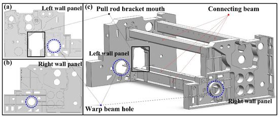
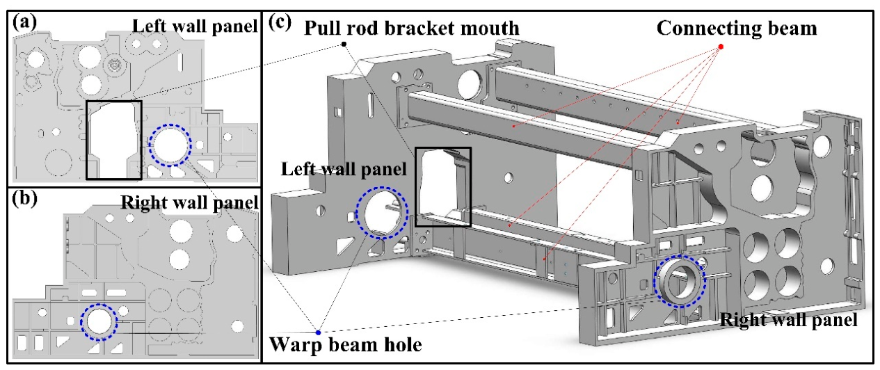
The structural design focuses on the jet loom frame, as shown in Figure 1. It clearly defines the loads the frame must bear (static and dynamic loads) and dimensional constraints. Considering the static and dynamic loads borne by the frame and the dimensional constraints, the wall panel and beam models are designed by the SolidWorks software 2022 [26]. Then, the cross-sectional shape of the beam is determined after taking into account the connection between the beam and the wallboard.
Figure 1.
Structural design of the jet loom frame. (a) left wall panel; (b) right wall panel; (c) pull rod bracket mouth.
2.2. Finite Element Model Building
The frame 3D model is imported into ANSYS Workbench software 2022R2 for finite element preprocessing [27]. The materials of the wall panels, beams, and other parts are Q345B, HT300, and QT500-7, respectively. The main mechanical properties of the loom frame are as follows in Table 1. To enhance the simulation efficiency, excessively small holes that are non-stressed are overlooked. The model is meshed using tetrahedral elements [28]. To balance computational efficiency and accuracy, the grid size of critical regions (e.g., beam connections, load application points) is refined to 10 mm, while other regions mesh to 15 mm.
Table 1.
Material property table.
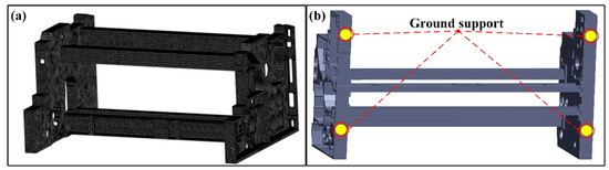
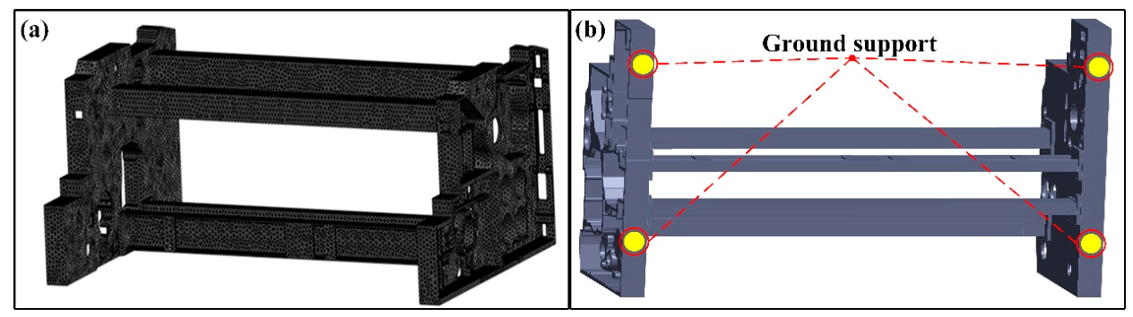
The total elements number is approximately 120,000, and the nodes number is around 250,000. The meshed finite element model of the jet loom is shown in Figure 2a.
Figure 2.
Mesh division and boundary conditions of the jet loom frame: (a) Mesh division, (b) boundary conditions.
2.3. Model Verification and Validation
Modal analysis is recognized as one of the most effective methods for investigating the dynamic characteristics of structures [29], and each mode is associated with a specific natural frequency and mode shape that reflect the inherent vibration properties of the mechanical structure.
2.3.1. Modal Simulation and Experiment Design of the Jet Loom Frame
After the loom frame modeling procedure is completed, the appropriate boundary conditions are applied in the modal simulation. The bolt hole area connected to the ground is fully constrained, limiting displacement and rotational degrees of freedom, as shown in Figure 2b, while other parts remain free. The connections between the wall panels and the beams are defined as face-to-face contact, and fixed support constraints are imposed at the hole locations at the bottom of the wall panels. A weak spring option is activated to prevent convergence issues caused by the excessive displacement deformation of the exciter. Following preprocessing, the modal simulation is performed using the Block Lanczos algorithm [30].
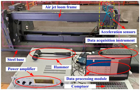
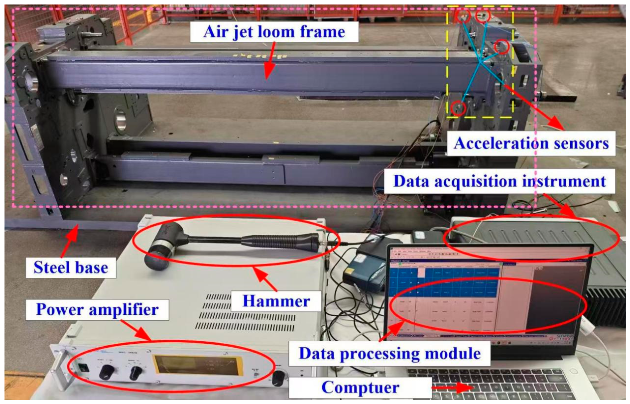
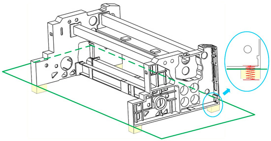
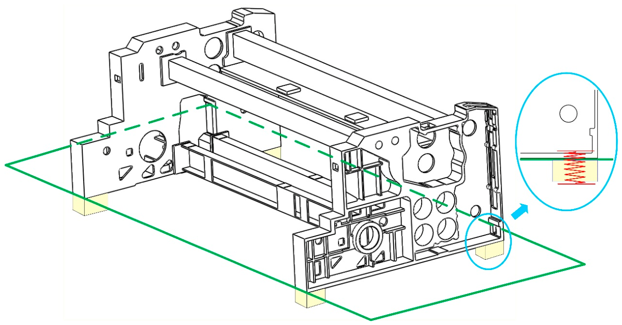
The modal experiment scene of the jet loom frame is illustrated in Figure 3. The frame is securely bolted onto a steel testing platform to simulate actual installation conditions. Shock absorbers in Figure 4 are placed at the bottom to more accurately reflect the true working condition of the frame. The vibration signals are captured by accelerometers attached to the surface of the air-jet loom frame. The received signals are processed by Siemens Test Lab software 2021.2. Siemens Test Lab software is used for data acquisition and analysis [31]. In the model experiment, the PCB hammer 086D20 is used to strike the frame to simulate impact loads. The acceleration sensors are three-axis accelerometers manufactured by PCB Company (Buffalo, NY, USA) of the United States, model TLD356A16. A total of 16 sensors are deployed and installed at different test points in turn for measurement. The Siemens data acquisition system (LMS SCADAS Mobile SCM05) monitors (Leuven, Belgium) and acquires the time-domain signals of the system. The sampling frequency is set to 1024 Hz, and the sampling time for each test ranges from 15 to 20 s. At each measuring point, five valid hammer impacts are conducted, and linear averaging is adopted to process frequency response functions. These settings comply with the conventional specifications for modal testing of medium-sized mechanical structures. Data recording and analysis are completed via the Impact Testing module in Testlab2021.1. The Poly Max algorithm embedded in the Siemens Impact Test module is used to identify the first six vibration modes and natural frequencies of the rack.
Figure 3.
Modal experiment scene of the jet loom frame.
Figure 4.
The shock absorber of the air-jet loom frame system. (Green line is used as the base plate to place the rack).
2.3.2. Modal Results Analysis of the Jet Loom Frame
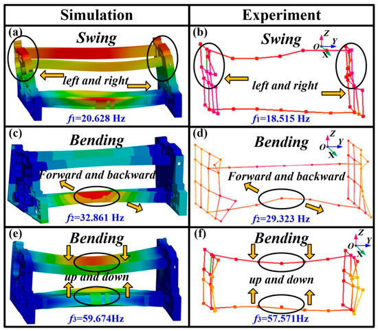
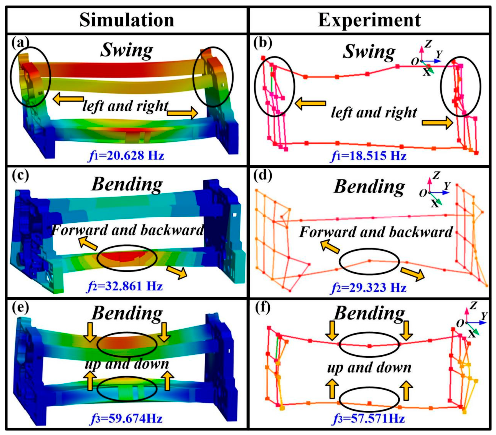
The simulation and experimental results of the first three modes are shown in Figure 5. Figure 5a,c,e show the modal simulation results of the loom frame, while Figure 5b,d,f show those of the experimental outcomes. The wall panels of the loom frame swing along the Y direction in the first simulation and experiment mode shapes. Meanwhile, the upper beams swing in phase with the wall panels, and the lower beams experience slight deformation in Figure 5a,b. The first-order natural frequency from the simulation and experiment are 20.628 Hz and 18.515 Hz, respectively. In the second simulation and experiment mode shapes from Figure 5c,d, the lower beam of the jet loom frame undergoes compression and tensile bending deformation along the X direction forward and backward, while the rear ends of the side wall panels contract and bend inward. The second-order natural frequency from the simulation and experiment are 32.861 Hz and 29.323 Hz. It can be seen in Figure 5e,f that the upper and lower beams bend up and down along the Z direction in the third mode shape. However, the wall panels on both sides have not undergone significant deformation. The third-order natural frequency from the simulation and experiment are 59.674 Hz and 57.571 Hz.
Figure 5.
Comparison of the modal experimental and simulation results: (a,c,e) are simulation results; (b,d,f) are experiment results.
Furthermore, the first six modal frequencies are shown in Table 2. The nonlinear damping effects and energy dissipation in the actual structure are not taken into account during the linear simplification process in the simulation model. Therefore, the simulation results are generally slightly higher than the experimental values. However, the natural frequency errors are around 10% within an acceptable range. Overall, the loom frame modal frequencies and shapes from simulation and experiment exhibit excellent consistency, which indicates the accuracy of the dynamic model.
Table 2.
Modal frequencies of the simulation and experiment.
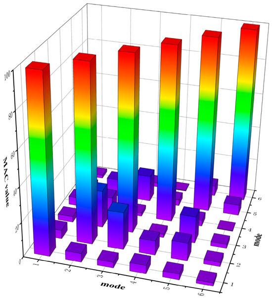
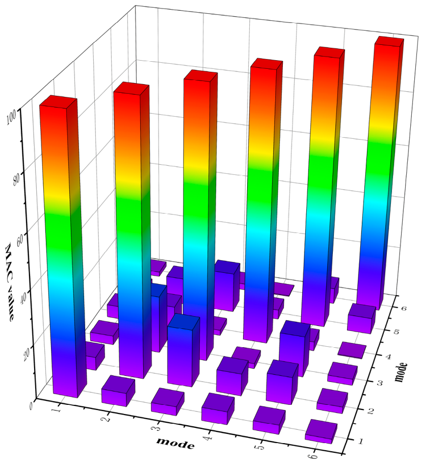
The diagonal values of the MAC matrix in Figure 6 are close to 1, and the off-diagonal values are close to 0, indicating a high consistency between experimental and simulated mode shapes and good orthogonality of each order mode, which also verifies the accuracy of the finite element model.
Figure 6.
First six modal MAC matrix.
3. Jet Loom Frame System Vibration Testing and Analysis
3.1. Vibration Testing Experiment
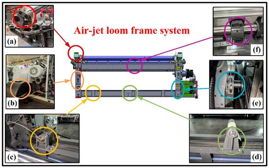
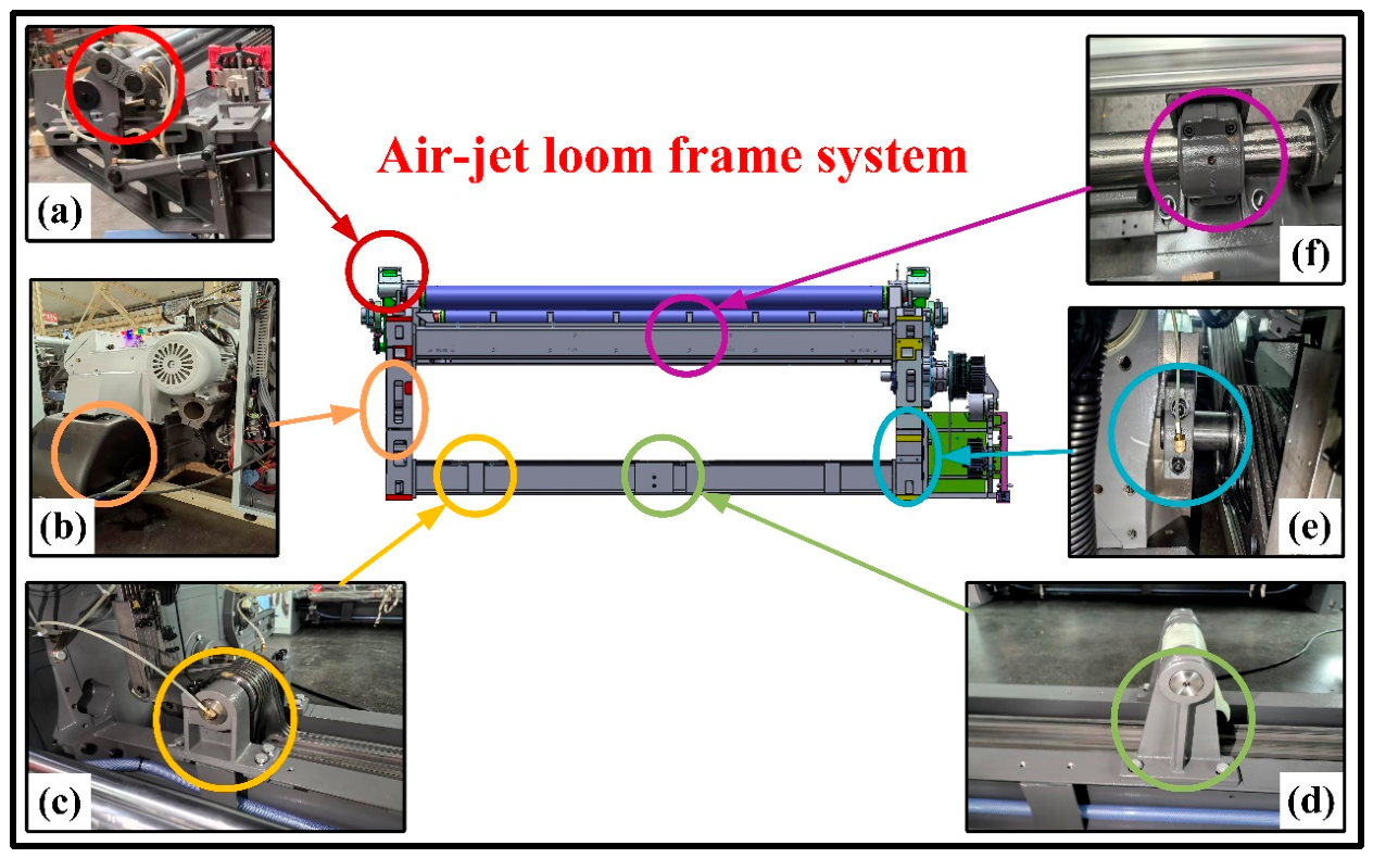
In order to further study the dynamic characteristics of the loom frame under working conditions. The test system of the modal test is used in the vibration test again, by which the vibration acceleration signals in the X, Y, and Z directions at each measuring point are collected. The tests are performed under normal operation within the common production speed range of 600–1000 rpm. As shown in Figure 7, the primary sources of vibration in the frame [32] can be categorized into the beating up rocker mechanism, the opening mechanism, the let off link mechanism, and the tie rod mechanism. The beating up rocker mechanism is the core component to realize “beating up and forming cloth”. It drives the reed to push the weft yarn to the weaver mouth through the reciprocating swing of the reed. When the reed swings, it produces significant inertia force. At the same time, the impact load will be formed by the impact of the reed with the weft and warp yarns. The opening mechanism creates a shed for the weft yarn to pass through by raising and lowering the heddle frame. This motion must overcome the resistance caused by the tension in the warp yarn, and the periodic fluctuation in warp yarn tension applies alternating forces to the mechanism, which are transmitted to the frame. The let off link mechanism releases the warp from the weaving shaft smoothly through the uniform rotation of the let off roller. The core is to maintain the constant tension of the warp. The tie rod mechanism is the power transmission link connecting various actuators and the main drive system. Fluctuations in the output torque of the main drive motor are transmitted to each mechanism through the tie rod, causing the tie rod to generate torsional vibration. The asynchronous movement of each mechanism will cause the tie rod to bear additional bending moment, resulting in lateral vibration.
Figure 7.
Schematic diagram of vibration sources of the whole machine: (a) let off link support, (b) opening mechanism support, (c) left tie rod support, (d) middle tie rod support, (e) right tie rod support, (f) beating up rocker support.
These main vibration sources as experimental objects from the jet loom are vibration-tested, and the acceleration results of each vibration source are obtained. Then, the accelerations at the above vibration sources are post-processed and used for the loading conditions of subsequent vibration simulation.
3.2. Jet Loom Frame Evaluation Point Vibration Analysis
3.2.1. Jet Loom Frame Evaluation Point
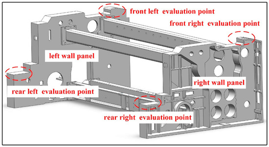
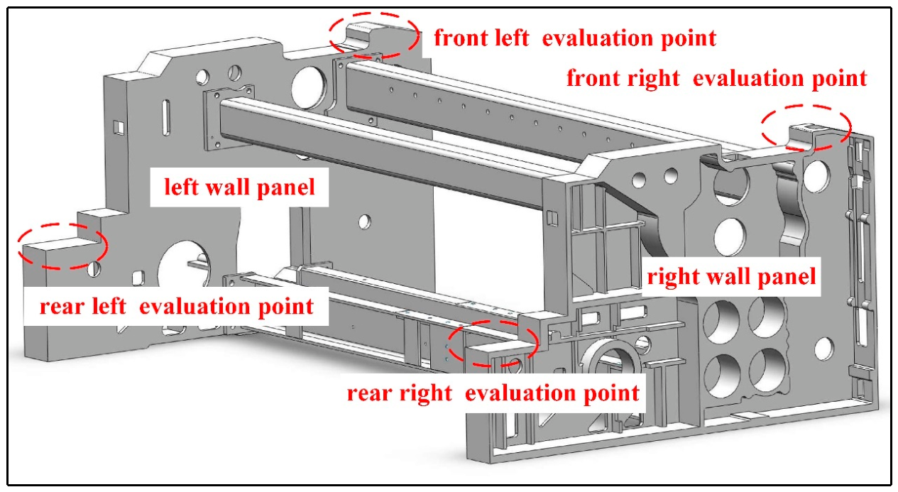
For the scientific evaluation of the vibration characteristics in the loom, the four key nodes are selected as the comprehensive evaluation points based on the present industry standards [33]. The above four vibration evaluation points locate in dynamically sensitive regions of the air-jet loom frame; the dynamic stability and system response with alternating loads can thereby be reflected by them under high-speed operation.
In terms of spatial arrangement, the four vibration evaluation points are symmetrically distributed at the four top corners of the frame at critical support locations, as shown in Figure 8. The left-front point and the right-front point are positioned adjacent to the support end of the beating-up mechanism to monitor the transient excitation induced by beating-up impacts on the front section of the frame and the lateral symmetry of the structure. The left-rear and right-rear points are located near the warp feeding mechanism to reflect the response characteristics of the frame rear section during long-period loads and the dynamic shift of the overall mass center. The complete vibration field mapping of the entire machine is constructed based on the four-point linkage evaluation scheme, which ensures that the experimental data effectively cover the core vibration regions of the frame system.
Figure 8.
Distribution of the four evaluation points.
3.2.2. Vibration Analysis of the Evaluation Points
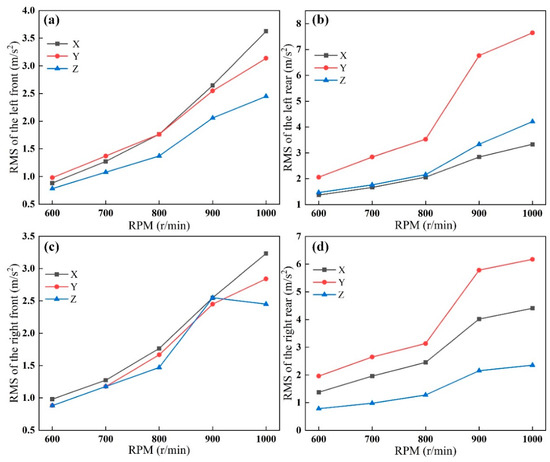
As illustrated in Figure 9, the vibration intensity at all evaluation points exhibits a pronounced increasing trend with the rise in the spindle rotational speed, indicating that the dynamic excitation forces are amplified in the high-speed operation. In particular, when the rotational speed reaches 900 r/min, the growth slope of the RMS (root mean square) values of the vibration acceleration in all directions becomes steeper, suggesting that resonance is induced at this operating speed. The rear evaluation points in Figure 9b,d show highly similar vibration characteristics at the left-rear and right-rear locations, with the vibration in the Y direction being the most severe. At 1000 r/min, the RMS value in the Y direction at the left-rear point approaches 8.0 m/s2, which is substantially higher than that in the X and Z direction. This result indicates that the lateral stiffness of the rear loom structure is relatively weak. Therefore, the vibration along the left-right direction of the loom is more easily excited under the lateral force components of the weft insertion or beating-up mechanism. The front evaluation points in Figure 9a,c display a relatively balanced vibration distribution at the front section, which is mainly governed by the combined effects of the X and Y direction. Among these components, the vibration in the X direction slightly exceeds the other directions after 900 r/min, which is primarily attributed to the forward and backward inertial impacts produced by the reciprocating motion of the beating-up mechanism. The comparison between the left-side and right-side evaluation point data indicates that the vibration responses of the loom exhibit good symmetry in the X and Y directions.
Figure 9.
Vibration data of the four evaluation points under different rotation speeds: (a) front left evaluation point, (b) rear left evaluation point, (c) front right evaluation point, (d) rear right evaluation point.
However, the vibration amplitudes at the rear section of the frame are significantly higher than those at the front section. Combined with the modal analysis results in Figure 5, this indicates that the overall modal shape of the frame oscillates along the Y direction. Meanwhile, the deformation amplitude at the rear of loom is greater than that at the front.
Furthermore, the RMS values of the Y direction at the rear section are also greater than that at the front end in the operating vibration test. Therefore, the results of modal and vibration testing exhibit excellent consistency, once again verifying the accuracy of the dynamic model.
3.3. Vibration Simulation of Loom
In order to carry out vibration simulation, the generalized acceleration of the system is obtained by combining the experimental acceleration signal with the kinematic mapping relationship, and then the dynamic external load excitation force is obtained by substituting it into the differential algebraic equation of multi-body dynamics. It can be directly used as a vibration source to load input in the simulation. All the multibody dynamics and inverse dynamics calculations in this section are implemented in MATLAB R2024a.
In the multibody system, the absolute acceleration of the measuring point and the generalized coordinates meet the kinematic mapping,
In Equation (1), is the acceleration of a point tested in the experiment, is the Jacobian matrix of the measuring point to the generalized coordinates, is the velocity coupling term, and are the generalized coordinates, generalized velocity, and generalized acceleration of the system respectively.
On the premise that the motion trajectories , are known, can inverse-solve the generalized acceleration from the measured acceleration:
In Equation (2), is the least square solution of the Jacobian matrix.
The generalized acceleration is substituted into the differential algebraic equation of multibody dynamics, and the Lagrange multiplier plus constraint form is adopted:
In Equation (3), is the system mass, is the complete constraint vector, is the constraint Jacobian matrix, is the constraint reaction vector, is the Coriolis force, centrifugal force, damping force, and other internal force items, and is the dynamic external excitation force.
The dynamic external excitation force can be obtained by inverse solution:
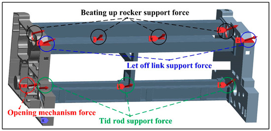
As shown in Figure 10, through the inversion of the above multi-body dynamics differential algebraic equation, the obtained dynamic external load excitation forces are applied to the corresponding support bearing seats and critical connection nodes of the frame, with the actual loading state of the loom simulated at the rotational speed of 600–1000 r/min. In parallel, in order to further enhance the structural strength of the air-jet loom frame, the intermediate support is introduced between the upper beam and the lower beam, which effectively improves the overall structural stiffness and the load-bearing capacity.
Figure 10.
Schematic diagram of the jet loom frame loading.
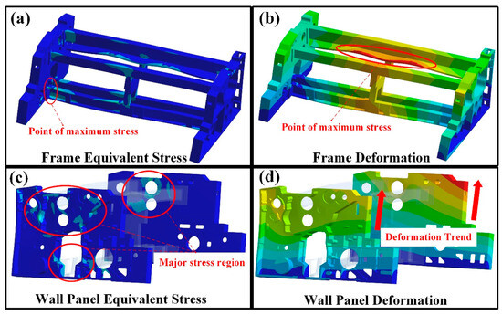
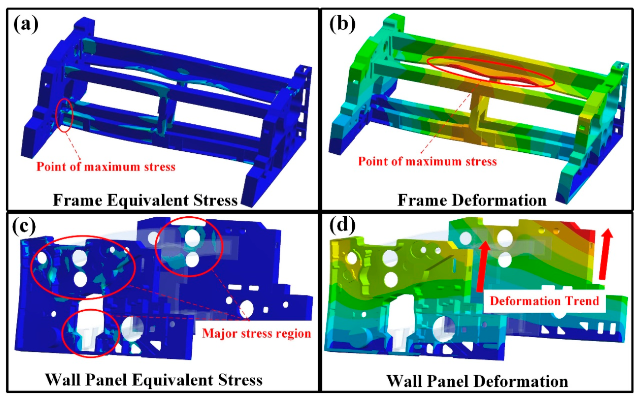
It can be seen in Figure 11a that the stress of the air-jet loom frame is mainly located at the connections between the beams and the wall panels, as well as at the connections between the intermediate support and up-low beams. Among these regions, the maximum stress occurs at the connection between the rear lower beam and the left wall panel, with the peak value reaching 36.992 MPa. Due to the vibration coupling effect between the connecting rod and cam box, this region becomes the core mechanically vulnerable zone of the frame. The maximum deformation of the air-jet loom frame is located at the connection between the upper front beam and the beating-up shaft, as shown in Figure 11b. This result further confirms that the beating-up shaft is the key excitation source during the operating state.
Figure 11.
Stress and deformation cloud diagrams of the frame at 900 RPM: (a) maximum stress cloud diagram of the frame, (b) maximum deformation cloud diagram of the frame, (c) maximum stress cloud diagram of the wall panel, (d) maximum deformation cloud diagram of the wall panel.
The primary stress concentration regions of the wall panels are illustrated in Figure 11c, where the high-stress zones are mainly distributed around the positioning holes for the beating-up shaft on the wall panels and the surrounding regions of the cam box. This distribution is directly associated with the fact that the beating-up shaft and the cam box are the two components exhibiting the most intense vibration within the frame. The transmission of vibrational loads is identified as the principal cause of the stress concentration in these regions. The deformation of the wall panels under operating load is presented in Figure 11d. Under the combined action of the bottom constraints and operating loads, the whole frame undergoes lateral swaying. When the height of the wallboard increases, the deformation becomes more pronounced, exhibiting a distinct layered characteristic. The maximum deformation area is located at the top of the wallboard.
In summary, the stress distribution of the frame is near several major vibration sources, while the overall deformation trend conforms to the laws of linear mechanics. The above results can provide mechanic evidence of the structural reinforcement design and vibration reduction measures.
3.4. Comparative Analysis Under Multiple Working Conditions
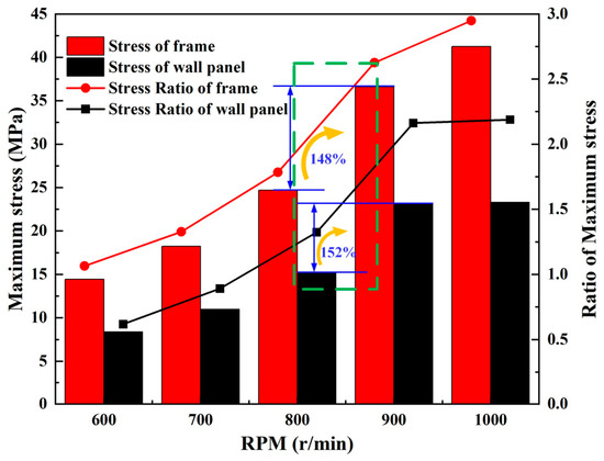
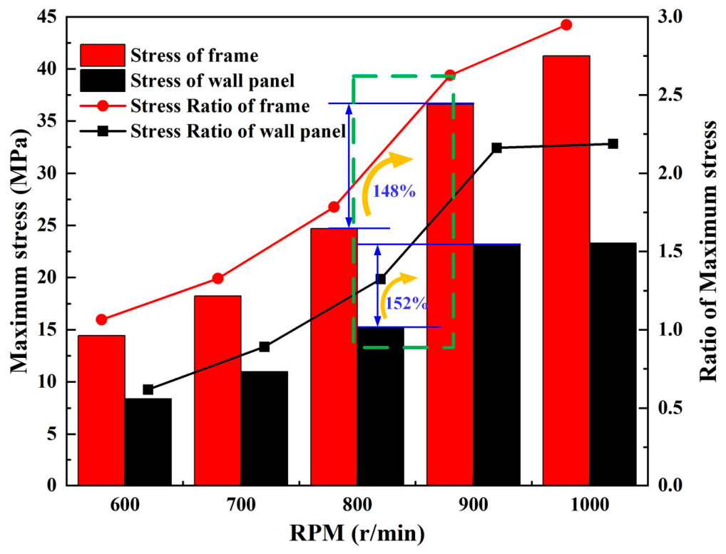
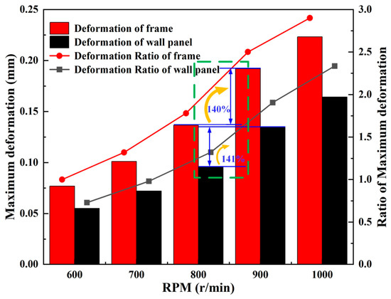
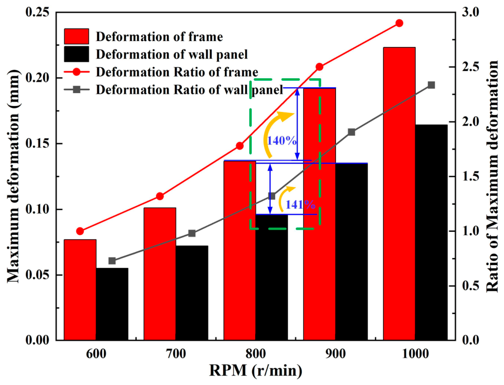
The stress and deformation analysis results of the frame in Figure 12 and Figure 13 indicate that the maximum stress and deformation of the frame and wall panel show a significant upward trend with the gradual increase in rotational speed. At the rotational speed of 900 r/min, the growth of both quantities reaches the maximum level among all operating conditions, indicating that the structural vibration is most severe and the dynamic response is most sensitive under this rotational speed. Therefore, the stress and deformation data obtained at the rotational speed of 900 r/min can be regarded as the key reference indices for the subsequent structural optimization, local reinforcement, and reliability assessment. The above results provide theoretical and data-based support for the subsequent optimization of structural parameters.
Figure 12.
Stress comparison in the frame and wall panel under multiple conditions. (The green box represents the most severe upward working condition).
Figure 13.
Deformation comparison in the frame and wall panel under multiple conditions. (The green box represents the most severe upward working condition).
4. Optimization of the Improved BA-HHO-SVR Model
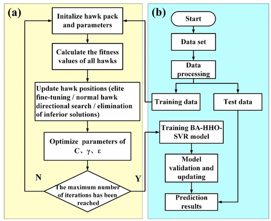
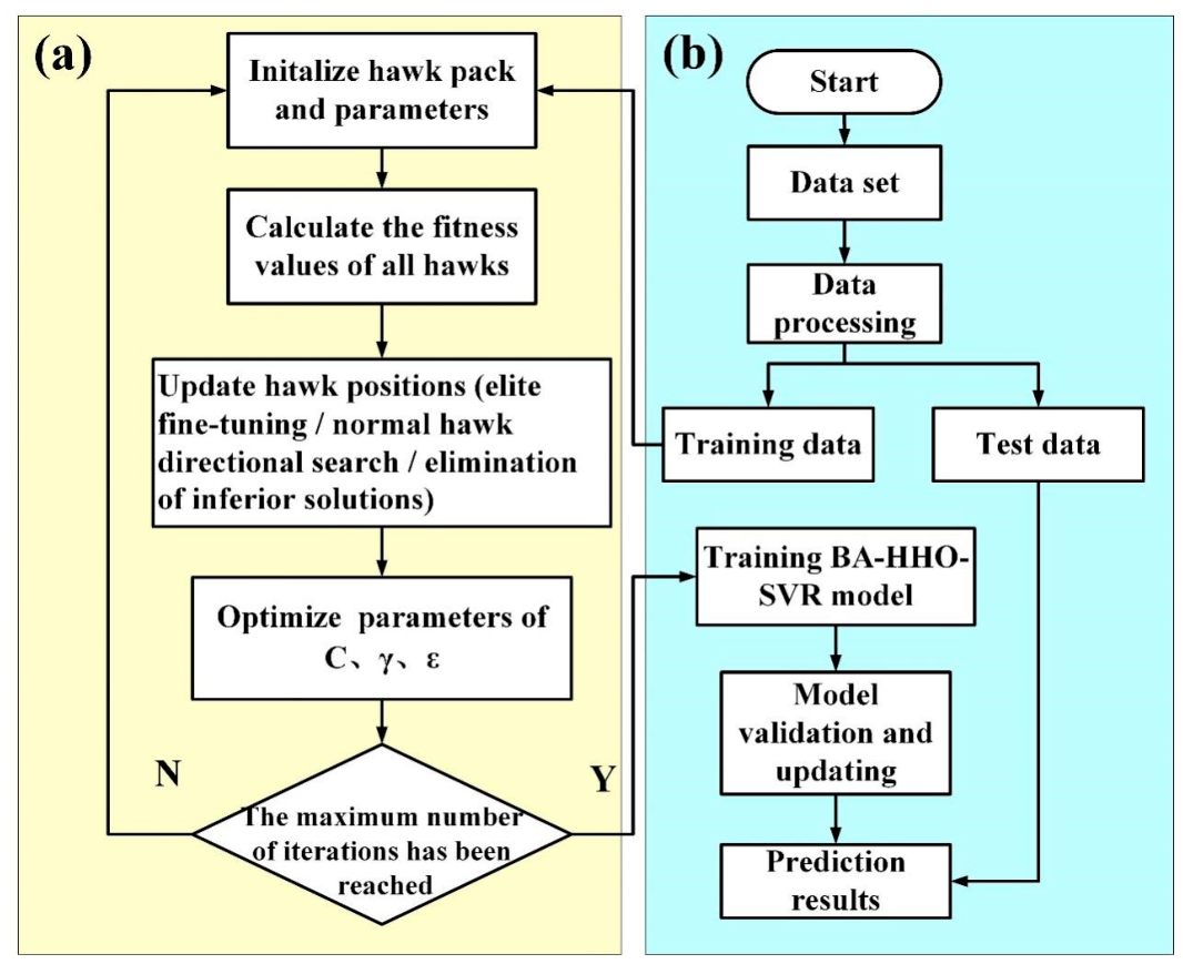
This optimization effort constructed a multi-model integrated stress prediction and optimization system in Figure 14. Its primary functions include predicting stress values through multiple machine learning and deep learning models, enhancing model performance using optimization algorithms, and further identifying the optimal input parameters corresponding to minimum stress. The model compares three foundational surrogate models—BP, RF, and SVR—and selects SVR as the optimal base model. It then employs both the HHO-SVR optimization model and the improved BA-HHO-SVR optimization model for minimum stress prediction. This validates the superiority and reliability of the improved BA-HHO-SVR optimization prediction model in minimizing stress values, offering an efficient and dependable novel prediction method for minimum stress assessment.
Figure 14.
Flowchart of the BA-HHO-SVR optimization steps: (a) data preprocessing (light yellow); (b) model training, validation, and prediction (light blue).
4.1. Principles of Support Vector Regression
Support Vector Regression (SVR) is a regression algorithm based on Support Vector Machines. Its core principle involves constructing a separating hyperplane by identifying support vectors, thereby enabling the modeling of uncertain functional relationships [34].
The mathematical model of SVR can be expressed as
In Equation (5), represents the predicted value of the output variable, denotes the input variable, is the weight vector, is the function mapping the input variable to a high-dimensional space, and is the bias term.
The objective of SVR is to minimize the number of support vectors and the distance to the hyperplane, which can be formulated as an optimization problem:
In Equation (6), > 0 is the penalty coefficient that balances hyperplane complexity and out-of-band sample loss. and are slack variables used to control the number of support vectors. Equation (7) represents the constraint condition: a larger imposes heavier penalties on out-of-band samples, enhancing the model’s fitting capability but increasing the risk of overfitting; a smaller yields a simpler model prone to underfitting.
4.2. Harris Hawks Optimization
Mirjalili et al. proposed Harris Hawks Optimization (HHO) in 2019, a swarm intelligence optimization algorithm that mimics the natural hunting behavior of Harris hawks [35]. In order to efficiently search for global optimal solutions to optimization problems, its fundamental mechanism entails mimicking the behavioral patterns of Harris hawks during their exploration phase and exploitation phase. The algorithm strikes a balance between local exploitation capabilities and global exploration through dynamic adjustments of energy factors and ambush strategies, which makes it appropriate for situations like function optimization and model parameter tuning. Every Harris hawk individual in HHO represents a potential solution to the optimization problem. The population size is recorded as , and the position vector of the th individual when the number of iterations is t is expressed as
In Equation (8), where denotes the dimension of the optimization variable, the prey position corresponds to the current optimal solution .
During the exploration phase, the Harris hawk performs random searches for prey by dynamically switching between two strategies: one based on the population’s average position and the other based on a random walk using Levy flight. This switching is controlled by a random number (). The position update equation is
In Equation (9), represents the average position vector of the population at time ; are energy factors during the exploration phase, ( represent different values of ), linearly decreases from 2 to 0 with the iteration count, and is a random vector; is the perception factor, ( is a random vector), simulating the eagle’s perception of prey; is the Levy flight random vector, expressed as , , , and are random vectors.
Upon detecting prey, the predator enters the development phase. The prey’s state is determined by the energy factor (, ): indicates low prey energy, triggering a hard-enveloping strategy. Simultaneously, the ambush factor () activates different attack modes.
The prey is not fully surrounded. The hawk gradually approaches the prey. The position update formula is
In Equation (10), represents the logarithmic spiral shape factor (typically set to ), is a random vector, and simulates the spiral trajectory of a hawk circling its prey.
The prey is completely surrounded, and the hawk launches an attack. Based on the ambush factor , two modes are distinguished:
In Equation (11), represents the random jump factor (), simulating the sudden turns during an eagle’s attack; is a random vector enhancing the randomness during the attack phase; when , it constitutes a gradual attack, while indicates a surprise attack, utilizing the population’s average position to disrupt the prey.
The algorithm iteratively updates the positions of individuals until the maximum iteration count is reached. At this point, represents the optimal solution to the optimization problem.
4.3. BA-HHO-SVR Algorithm: Improved Harris Hawks Optimization
The BA-HHO algorithm adopts the core theory of cooperative hunting by Harris hawk flock. Based on the original HHO framework, the guidance mechanism, search strategy, and population evolution logic have been optimized to enhance the accuracy and efficiency of support vector regression (SVR) parameter optimization.
Split the dataset into a training set and a test set. Initialize the core parameters of the BA-HHO algorithm, including the lower and upper bounds (), population size (), problem dimension (), and maximum iterations () (Improvement 1: Focused Initialization). To avoid excessive dispersion of the initial population, the initialization search range is contracted to 50% of the total range . The initial positions are generated using Equation (12):
This strategy reduces ineffective early-stage search and guides the population to quickly cluster towards high-quality solution regions.
The SVR model is trained using the training samples and calculates the fitness value for each Harris hawk individual, such as the cross-validation RMSE (Improvement 2: Multi-Elite Cooperative Guidance). Instead of the single-elite guidance in the original HHO, this step screens the top 30% of individuals with the best fitness to form the Elite Hawk Group () while retaining the global optimal individual as the Main Leader (). The risk of local optima is reduced and the search diversity is enhanced based on the multi-elite fusion method.
Execute the position update based on defined dual decay factors and the step decay factor:
Equation (13) is applied to the local fine-tuning and the exploration intensity factor.
Equation (14) is applied to directed perturbation.
The population updates are performed in three hierarchical layers.
(Improvement 3: Elite Fine Hunting) Elite hawks perform autonomous fine-tuning on their superior positions:
Equation (15) is applied to preserve unique search directions.
(Improvement 4: Directed Search) Common hawks select a random elite () as an anchor for directed search with dynamic perturbation:
Equation (16) is applied to balance global search with local refinement.
(Improvement 5: Elimination Mechanism) The bottom 20% of hawks with the worst fitness are eliminated and replaced by mutated variants of random elites:
The Equation (17) is applied to optimize the overall population quality.
Recalculate the fitness values of all hawks after the iteration. Compare the fitness of the current individuals with the global Main Leader (). If a current hawk demonstrates superior fitness to the Main Leader, update the global optimal position () and optimal fitness () to the current individual’s state; otherwise, keep them unchanged.
Check if the termination conditions are met. If the maximum iteration count () is reached or the Main Leader’s fitness satisfies the preset precision requirement, terminate the iteration. Output the optimal parameter combination (), the best fitness value (), the optimization time, and the convergence curve data comprising the optimal fitness of each gene ration.
4.4. Construct Optimization Model
4.4.1. Model Parameterization
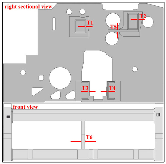
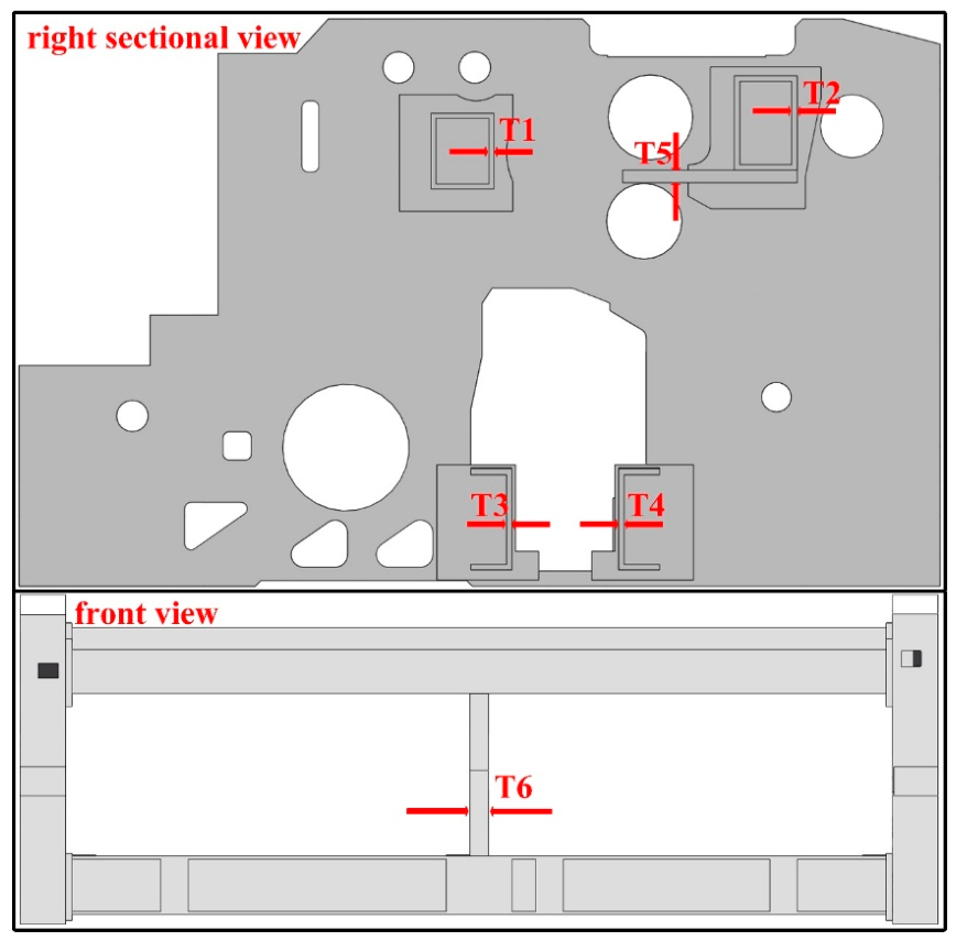
According to the dynamic research results in Section 3.3 above, it is found that the stress and deformation are mainly caused by the overall left–right swing of the frame. The fundamental reason for the above deformation is the insufficient stiffness of the beam. Therefore, the support stiffness of the strengthened beam is selected as the optimization parameter. This study selects six key features in Figure 15—upper rear beam thickness (), upper front beam thickness (), lower rear beam thickness (), lower front beam thickness (), intermediate support thickness (), and weft-insertion shaft support plate thickness ()—as evaluation indicators for predicting minimum stress values. Among these, the thicknesses of the upper rear beam, upper front beam, lower rear beam, and lower front beam reflect the overall influence of the beams on the wall plate; the middle support thickness indicates the support’s influence on beam stability, while the lower beam rib thickness represents the impact of enhanced beam stiffness on overall stability. Five-level values are obtained for each factor, with the parameter level factor table shown in Table 3. Based on the selected evaluation indicators, an input parameter dataset is established using the Central Composite Design method and Variance Inflation Factor optimality design [36]. Dynamic simulation in ANSYS Workbench 2022R2 then yields stress values corresponding to each parameter set.
Figure 15.
Optimize size selection.
Table 3.
Parameter Level Factor Table.
Grey relational analysis is employed to validate the correlation between equivalent stress and five sets of weaving machine frame structural parameter combinations: upper rear beam thickness, upper front beam thickness, lower rear beam thickness, lower front beam thickness, intermediate support thickness, and weft-insertion shaft support plate thickness. The grey correlation results between the five loom frame parameter combinations and equivalent stress are shown in Table 4. It can be observed that under different loom frame parameter combinations, all six input parameters exhibit high grey correlation with equivalent stress. Therefore, the grey correlation analysis results indicate that the thickness of the upper rear beam, the thickness of the upper front beam, the thickness of the lower rear beam, the thickness of the lower front beam, the thickness of the middle support, and the thickness of the weft-insertion shaft support plate can be used as input features to form a dataset for predicting the equivalent stress of the air-jet loom frame.
Table 4.
Grey Correlation Coefficients Between Input Parameters and Equivalent Stress.
4.4.2. Model Evaluation Criteria
To evaluate the accuracy of the established predictive model, the following metrics are used: R-squared (R2), Mean Absolute Error (MAE), and Root Mean Square Error (RMSE). The calculation formulas are as follows:
:
MAE:
RMSE:
In Equations (18)–(20), denotes the total prediction time length, while , , and represent the actual value, predicted value, and average actual value of the equivalent stress, respectively.
4.4.3. Parameter Settings
A predictive model is established based on the above stress dataset. The dataset is randomly split into a training set and a test set, comprising 70% and 30% of the total data, respectively. Six key features—upper rear beam thickness (), upper front beam thickness (), lower rear beam thickness (), lower front beam thickness (), middle support thickness (), and beating-up shaft support plate thickness ()—are used as model inputs, with equivalent stress as the model output. The parameter settings for the optimization model are shown in the table. In the SVR model, the initial penalty coefficient and kernel function are set as follows: C = 2, gamma = 0.1, epsilon = 0.1. The population size for both HHO-SVR and BA-HHO-SVR optimization models is 20, with a maximum iteration count of 200. The number of variables is three, the parameter lower bounds are [1, 0.001, 0.01], and the parameter upper bounds are [500, 5, 0.3], as detailed in Table 5.
Table 5.
Optimized Parameter Settings.
4.4.4. Analysis and Comparison of Optimization Models
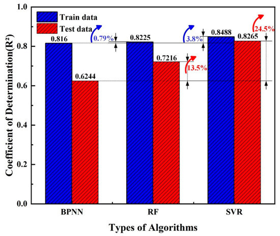
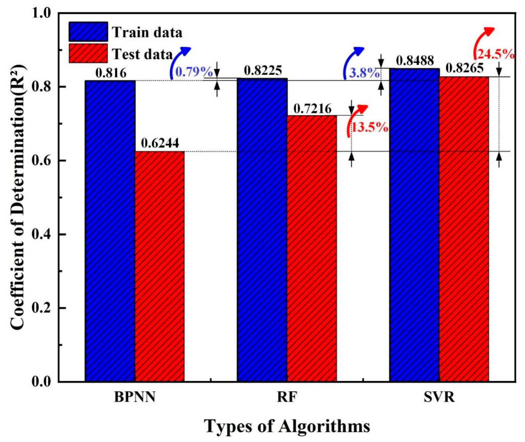
The predictive performances of the three basic algorithms, BPNN, RF, and SVR, are shown in Figure 16, which reveal significant differences in how each model handles the dataset used in this study. In terms of prediction accuracy, SVR (Support Vector Regression) demonstrates the best overall performance, achieving a training set R2 of 0.8488 and a test set R2 of 0.8265. Compared to BPNN and RF, its test set accuracy increases by 24.5% and 13.5%, respectively, validating the algorithm superiority in characterizing complex nonlinear mapping relationships. From the perspective of generalization capability, although BPNN performs reasonably well on the training set (R2 = 0.816), it exhibits a noticeable performance drop on the test set (decreasing to 0.6244). This reflects the model tendency toward overfitting and generalization bottlenecks under the current sample size. In contrast, SVR demonstrates the highest consistency between internal and external errors, showcasing excellent robustness. In summary, the SVR algorithm leverages its adherence to the structural risk minimization principle to achieve both high fitting accuracy and more stable extrapolation capabilities. Therefore, the SVR algorithm is selected as the baseline model for subsequent optimization design in this research.
Figure 16.
Predictive performances of three basic algorithms.
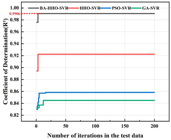
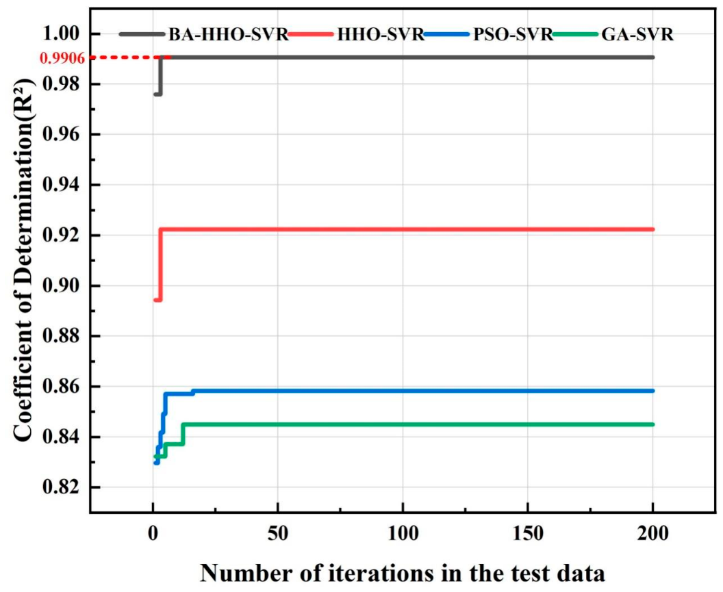
To thoroughly analyze the performance boundaries of the proposed improved model in tackling complex regression problems, this paper compares the iterative characteristics and final predictive efficacy of SVR models driven by different optimization algorithms, as shown in Figure 17. At the algorithmic evolution level, the convergence curves on the left clearly demonstrate the BA-HHO-SVR model’s superior performance in solution space exploration. Benefiting from the enhanced global exploration capability of the Harris Hawk Optimization (HHO) algorithm through the improved algorithm (BA) strategy, the enhanced model effectively overcomes the limitation of traditional PSO-SVR and GA-SVR models that are prone to local optima. Its final test set coefficient of determination is locked at 0.9906 in Table 6, demonstrating exceptionally high fitting consistency.
Figure 17.
Comparison of optimization algorithm performance iterations.
Table 6.
Comparison of Multi-Model Evaluation Metrics.
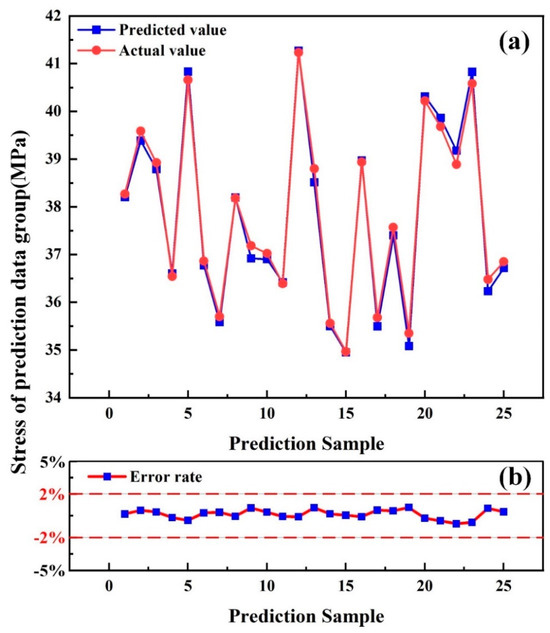
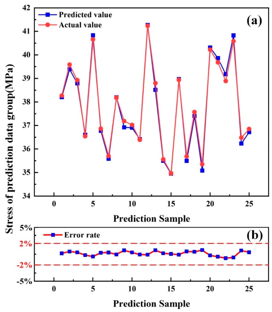
In practical prediction accuracy assessment, the predicted results of Figure 18a further demonstrate the high overlap between model predictions and experimental values. Beyond the R2 metric, calculations of absolute error indicators reveal that the BA-HHO-SVR model maintains extremely low levels of both Root Mean Square Error (RMSE) and Mean Absolute Error (MAE). This indicates the model not only accurately captures overall trends but also exhibits minimal numerical deviation at individual data points, effectively overcoming prediction lag or oscillation phenomena near extreme points that plague traditional models. As shown in Figure 18b, the prediction error rate across all samples strictly converges within a ±2% confidence interval, with no significant discrete outliers. This fully demonstrates that the improved algorithm significantly reduces the model generalization variance during the parameter refinement optimization process. In summary, the BA-HHO-SVR model maintains exceptional convergence accuracy while exhibiting robust numerical prediction stability and interference resistance. Its outstanding comprehensive performance provides a scientifically sound mathematical foundation for subsequent rack system parameter optimization.
Figure 18.
Comparison of the predicted results: (a) predicted and actual values, (b) error rate.
4.5. Optimization of Jet Loom Frame Parameters
4.5.1. Model Optimization and Solution
Optimization calculations are performed on the BA-HHO-SVR model to obtain the optimal parameter combination and corresponding equivalent stress. To further validate the computational accuracy of the BA-HHO-SVR optimization model, the four evaluated models are solved individually. Based on the solution results, the outcomes of each model are verified through finite element dynamic simulation.
The optimal structural parameter combinations of the four algorithms are presented in Table 7. It can be found that the equivalent stress with the BA-HHO-SVR optimized model is the minimum, which is only 33.0248 MPa. The optimal parameter combination for the BA-HHO-SVR optimized model is as follows: Upper rear beam thickness (): 16.1545 mm, Upper front beam thickness (): 12.0493 mm, Lower rear beam thickness (): 12.5620 mm, Lower front beam thickness (): 13.6456 mm, middle support thickness (): 100.8555 mm, beating-up shaft support plate thickness (): 25.1106 mm.
Table 7.
Optimal Parameter Combination.
4.5.2. Simulation Verification
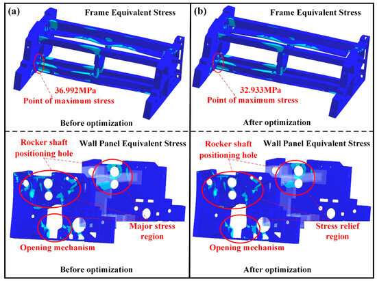
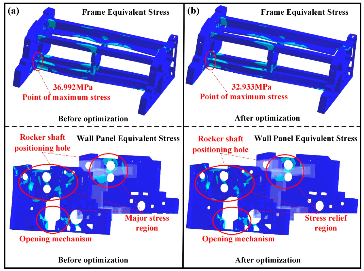
In terms of the actual optimization effectiveness, the stress contour plots in Figure 16 reveal that Figure 19a show the results before optimization, and Figure 19b show the results after optimization. It is found that the maximum stress of the whole loom frame occurs at the connection between the lower rear beam and the left wall panel. The maximum stress areas of the wall panel are around the rocker shaft positioning hole of the wall panel and the connection between opening mechanism and the wall panel. The maximum stress value is 36.992 Mpa before optimization and 32.933 Mpa after optimization. After optimization, the maximum stress is reduced by 10.9%. At the same time, the maximum stress area is reduced. This method improves the mechanical properties of the structure and effectively reduces the failure risk caused by local stress overload. It provides an efficient scientific method for the lightweight and reliability design of engineering components.
Figure 19.
Stress comparison before and after optimization: (a) before optimization, (b) after optimization.
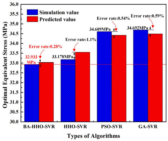
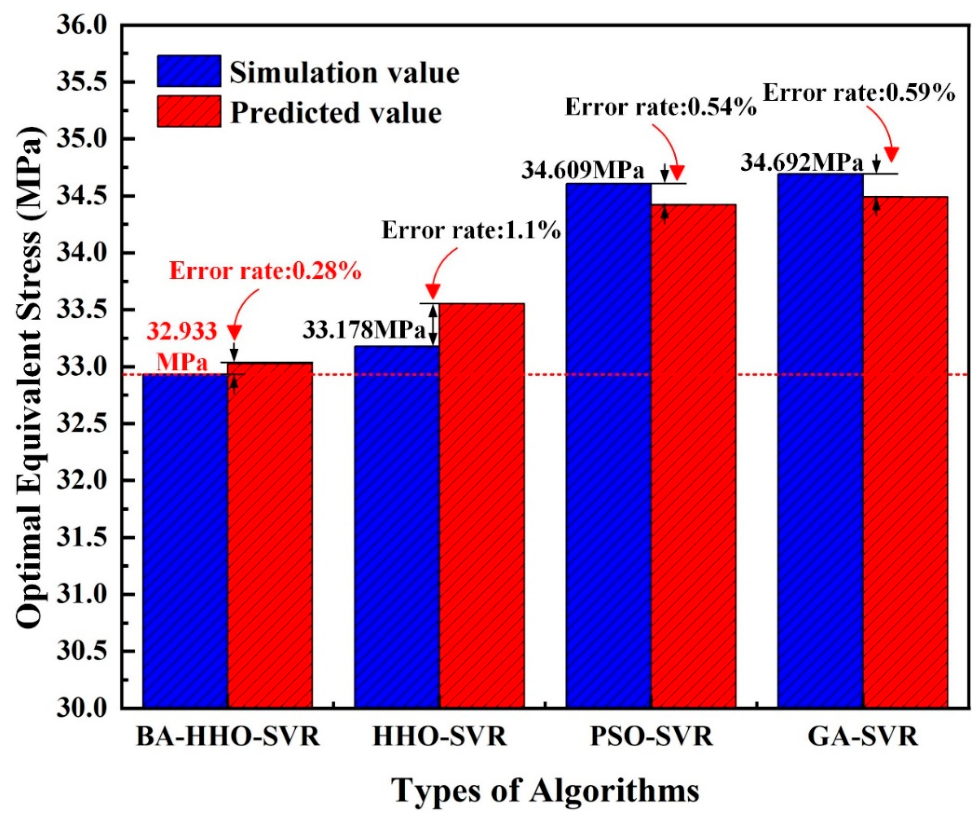
In order to further verify the superiority of the BA-HHO-SVR method, four algorithms are used for comparative verification. The comparison results of simulation and prediction are shown in Figure 20 and Table 8. The simulation stress value under the optimization result of BA-HHO-SVR method is the lowest, which is 32.933 Mpa. At the same time, the error value of simulation and prediction is the lowest among all algorithms, which is 0.28%. Therefore, the BA-HHO-SVR method shows better parameter search precision and solution space mapping ability and provides a solid high confidence index support for structural optimization design.
Figure 20.
Comparison of simulation and predicted values.
Table 8.
Simulation Verification and Error.
5. Conclusions
To address the structural strength issues of the air-jet loom frame system, this study carries out a systematic investigation including the frame system design and modeling, vibration testing and analysis, and structural parameter optimization. The main findings and conclusions are summarized as follows:
A modal simulation and experiment of the air-jet loom are conducted. The modal results indicate the frame model’s first natural frequency is 18.515 Hz, with the frame mode shape oscillating horizontally along the Y-axis. Furthermore, the first three natural frequencies and mode shapes of simulation show good consistency with the experiment results, which demonstrates the accuracy of the air-jet loom dynamic model.
Vibration test results under multiple operating conditions present that vibration values at evaluation points increase with operating speeds rising. The vibration amplitude of the loom escalates significantly at 900 RPM, where the corresponding frequency is close to the modal first natural frequency. Thus, the loom resonance speed can be identified at 900 RPM. Subsequently, the dynamic simulation is carried out based on the vibration test load under resonance speed. Dynamic simulation results indicate that the maximum stress of 36.992 MPa occurs at the connection between the rear lower beam and left side panel. Therefore, the stress value at 900 RPM is selected as the subsequent structural optimization target for the loom.
According to the dynamic analysis results, the loom frame structural parameter prediction model is constructed based on the BA-HHO-SVR method. After comparing evaluation metrics across multiple optimization models, it is found that the BA-HHO-SVR model achieves an R2 value of 0.9906, an RMSE of 0.1798, and an MAE of 0.1419. These results represent the highest values among all the various models, which demonstrates superior predictive performance and generalization capability in the BA-HHO-SVR model.
Structural parameter optimization of the loom frame is conducted based on the BA-HHO-SVR optimization model, yielding the optimal parameter combination under the minimum stress (33.0248 MPa). The above minimum stress is verified by dynamic simulation, and the error is only 0.28% between the prediction and simulation value. Furthermore, the optimized maximum equivalent stress value is significantly reduced by 10.9%. These results demonstrate that the BA-HHO-SVR model not only overcomes local optima traps effectively but also exhibits exceptional reliability in complex nonlinear engineering optimization problems. It provides a scientific basis for decision-making in designing lightweight and reliable high-performance loom structures.
The above researche on dynamic analysis and structural parameters optimization provide important theoretical support and reference for the optimization of the air-jet loom frame system.
Author Contributions
J.Z. and Z.C. designed and conducted the simulation and experiment and wrote the first draft of the article. S.L., L.Z., and F.H. conducted the data curation and experimental analyses. M.S., M.C., and F.F. contributed to the systematic review of the literature and the data retrieval and extraction. L.Y., C.W., and X.X. funded this research and provided all the experimental devices. All authors have read and agreed to the published version of the manuscript.
Funding
This work was funded by the Natural Science Foundation of Hubei Province under grant numbers 2025AFB365 and 2024AFB756; and the Key R&D Program of Shandong Province under grant number 2024CXGC010215; and the Science and Technology Research Project of Hubei Provincial Department of Education under grant number D20241603.
Data Availability Statement
Data are available on request.
Conflicts of Interest
There are no conflicts of interest to declare.
References
- Munck, D. The world market for looms. Ind. Text. 1993, 1246, 56–59. [Google Scholar]
- Nacmias, M. Somet presents its new Mythos air-jet loom. Text. Panam. 2000, 60, 74–78. [Google Scholar]
- Minoru, U. A Study on an Air-Jet Loom with Substreams Added. J. Text. Eng. 2006, 18, 106–113. [Google Scholar]
- Haifei, Q.I.U. Study on dynamic characteristics of air-jet loom frame structure. Silk 2019, 56, 32–35. [Google Scholar]
- Bílek, M.; Kovář, Š.; Skřivánek, J. Modal Properties of the Heald Frame of a Weaving Loom. Mech. Mach. Sci. 2022, 85, 289–295. [Google Scholar]
- Zou, H.; Song, J.; Wang, Z.; Chen, H. The effects of structural parameters on excitation force of airflow vibration piezoelectric generator. J. Vibroeng. 2018, 20, 2393–2402. [Google Scholar] [CrossRef] [Scilit]
- Kajiwara, I.; Agamatsu, A.; Seto, K. Technique of structural dynamic optimization using sensivities of resonance and anti-resonance frequencies. Am. Soc. Mech. Eng. Press. Vessel. Pip. Div. (Publ.) PVP 1989, 179, 161–167. [Google Scholar]
- Wolfrum, J.; Engelmann, J.; Weinsdorfer, H. Studies on improving the performance of high-speed jacquard weaving machines. Int. Text. Bull. 1998, 44, 69–76. [Google Scholar]
- Dividino, R.; Gottron, T.; Scherp, A.; Gröner, G. From changes to dynamics: Dynamics analysis of linked open data sources. In CEUR Workshop Proceedings; CEUR Workshop Proceedings: Aachen, Germany, 2014; Volume 1151. [Google Scholar]
- Buckley, N.W. Research on seismic structural optimization design based on performance-based design methods. Ing. Sismica 2025, 42, 1–18. [Google Scholar] [CrossRef] [Scilit]
- Qiu, H.; Chen, M.; Li, F.; Zhang, Y. Innovative design and experimental verification of cam shedding for high-speed looms. Alex. Eng. J. 2025, 112, 26–36. [Google Scholar] [CrossRef] [Scilit]
- Schwarzfischer, F.; Kurtenbach, S.; Onischke, J.; Corves, B. Design and Development of a Heddle Shaft Mechanism for Air-Jet Weaving Machines. Mech. Mach. Sci. 2017, 44, 23–28. [Google Scholar]
- Menglu, X.I.; Kaihong, Z.; Xin, L.U. Optimization of Motion Parameters and Structural Stiffness of Spatial Four-Bar Weft Insertion Mechanism of Rapier Loom. Mechanics 2023, 29, 511–517. [Google Scholar] [CrossRef] [Scilit]
- Eren, R.; Erturk, M.; Hascelik, B. Kinematic design and motion analysis of spatial rapier drive mechanisms used in weaving machines. Text. Res. J. 2014, 84, 2065–2073. [Google Scholar] [CrossRef] [Scilit]
- Lavrent’eva, E.P.; D’yachenko, V.V.; Mikahilova, M.P.; Koval’chuk, L.S. International exhibition of textile machinery ITMA-2011. Fibre Chem. 2012, 44, 135–140. [Google Scholar] [CrossRef] [Scilit]
- Mashroteh, H.; Mirjalili, S.A.M. Design and manufacturing an electromagnetic projectile mechanism for weft insertion in a loom. Qual. Text. Qual. Life 2004, 1–4, 1148–1152. [Google Scholar]
- Makarov, V.A.; Khozina, E.N.; Lebzak, A.B. Movement used in the drive of a loom shed-opening mechanism. Izv. Vyss. Uchebnykh Zaved. Seriya Teknol. Tekst. Promyshlennosti 2004, 6, 83–87. [Google Scholar]
- Sengupta, A.K.; Pratihar, P.; Kimothi, P.D.; Vernekar, S. Influence of yarn structure, sizing ingredients and type of sizing on properties and performance of sized yarns: Part III—A study of attrition during weaving for air-jet, ring and rotor yarns on a modern high speed weaving machine. Indian J. Fibre Text. Res. 2002, 27, 149–155. [Google Scholar]
- Abdulkareem, S.A.; Mustafa, Y.T.; Augustijn, E.W.; Filatova, T. Bayesian networks for spatial learning: A workflow on using limited survey data for intelligent learning in spatial agent-based models. GeoInformatica 2019, 23, 243–268. [Google Scholar] [CrossRef] [Scilit]
- Jian, W.; Wenyan, Y.; Daojian, C. Hybrid genetic–particle swarm algorithm: An efficient method for fast optimization of atomic clusters. Comput. Theor. Chem. 2015, 1059, 12–17. [Google Scholar] [CrossRef] [Scilit]
- Tsiptsis, I.N.; Liimatainen, L.; Kotnik, T.; Niiranen, J. Structural optimization employing isogeometric tools in Particle Swarm Optimizer. J. Build. Eng. 2019, 24, 100761. [Google Scholar] [CrossRef] [Scilit]
- dos Santos, A.T.; Carrer, J.A.M. Integrating GA-BEM and polynomial fitting for efficient structural shape optimization. Eng. Anal. Bound. Elem. 2025, 171, 106105. [Google Scholar] [CrossRef] [Scilit]
- Hao, J.; Yao, Z.; Hua, C.; Yu, C.; Li, C. Bending-torsional coupling vibration characteristics of asynchronous motorized spindle considering electromechanical coupling and multi-excitation effect. Mech. Syst. Signal Process. 2024, 208, 111039. [Google Scholar] [CrossRef] [Scilit]
- Masching, H.; Bletzinger, K.U. Parameter free structural optimization applied to the shape optimization of smart structures. Finite Elem. Anal. Des. 2016, 111, 33–45. [Google Scholar] [CrossRef] [Scilit]
- Bai, Y.; Grigoriadis, K.M. Damping parameter design optimization in structural systems using an explicit H∞ norm bound. J. Sound Vib. 2009, 319, 795–806. [Google Scholar] [CrossRef] [Scilit]
- Salahuddin, M.B.M.; Atikah, A.F.; Rosnah, S.; Zuhair, M.N.M. Conceptual design and finite element analysis of a high inclusion dough shaping machine using 3D-computer aided design (CAD) (SolidWorks)Konzeptionelles Konstruieren und Finite-Elemente-Analyse einer hochwertigen Teigformmaschine mit 3D-CAD (SolidWorks). Mater. Werkst. 2019, 50, 267–273. [Google Scholar] [CrossRef] [Scilit]
- Bakhtiar, B.; Yang, S.C.; Hsu, C.M.; Fan, K.K.; Yang, C.F. Using ANSYS Workbench as a Tool to Simulate and Analyze the Effects of Different Loads on Single-layer Reticulated Aluminum Domes. Sens. Mater. 2023, 35, 1715–1730. [Google Scholar] [CrossRef] [Scilit]
- Kulikov, I.M. On a Computational Model of Gravitational Hydrodynamics with Consideration of Radiation Transfer in the Diffusion Approximation Using Tetrahedral Meshes. J. Appl. Ind. Math. 2021, 15, 277–284. [Google Scholar] [CrossRef] [Scilit]
- Feron, J.; Latteur, P.; Pacheco de Almeida, J. Static Modal Analysis: A Review of Static Structural Analysis Methods Through a New Modal Paradigm. Arch. Comput. Methods Eng. 2024, 31, 3409–3440. [Google Scholar] [CrossRef] [Scilit]
- Dahmani, L.; Khennane, A.; Kaci, S. Crack identification in reinforced concrete beams using ANSYS software. Strength Mater. 2010, 42, 232–240. [Google Scholar] [CrossRef] [Scilit]
- Lei, S.; Mao, K.; Li, L.; Xiao, W.; Li, B. Sensitivity analysis of modal assurance criteria of damped systems. J. Vib. Control 2017, 23, 632–644. [Google Scholar] [CrossRef] [Scilit]
- Wei, F.; Shouwei, Z.; Sheng, W. Vibration test analysis and structure optimization for LL680 flexible rapier loom cam box. Key Eng. Mater. 2015, 670, 214–219. [Google Scholar]
- Iida, H.; Nakazawa, M.; Koike, S. Active Noise Control of a Moving Evaluation Point in One Dimensional Acoustic Field (2nd Report, Proposal of an Improved Noise Controller Applicable to a Rapid Moving Evaluation Point). Trans. Jpn. Soc. Mech. Eng. Ser. C 2001, 67, 2521–2527. [Google Scholar]
- Acosta, S.M.; Amoroso, A.L.; Sant’Anna, Â.M.O.; Junior, O.C. Predictive modeling in a steelmaking process using optimized relevance vector regression and support vector regression. Ann. Oper. Res. 2022, 316, 905–926. [Google Scholar] [CrossRef] [Scilit]
- Ibrahim, A.; Ali, H.A.; Eid, M.M.; El-kenawy, E.S.M. Chaotic Harris Hawks Optimization for Unconstrained Function Optimization. In 2020 16th International Computer Engineering Conference (ICENCO); IEEE: New York, NY, USA, 2020; pp. 153–158. [Google Scholar]
- Kohei, F.; Shun, M. Prediction variance of a central composite design with missing observation. Commun. Stat. Theory Methods 2020, 49, 6016–6031. [Google Scholar]

Disclaimer/Publisher’s Note: The statements, opinions and data contained in all publications are solely those of the individual author(s) and contributor(s) and not of MDPI and/or the editor(s). MDPI and/or the editor(s) disclaim responsibility for any injury to people or property resulting from any ideas, methods, instructions or products referred to in the content. |
© 2026 by the authors. Licensee MDPI, Basel, Switzerland. This article is an open access article distributed under the terms and conditions of the Creative Commons Attribution (CC BY) license.