Active Disturbance Rejection Control Based on Modified Particle Swarm Optimization of Six-Pole Hybrid Magnetic Bearing

Abstract

In order to solve the coupling problem of the six-pole hybrid magnetic bearing (SHMB), an active disturbance rejection control based on modified particle swarm optimization is proposed. Firstly, the active disturbance rejection control (ADRC) for the six-pole hybrid magnetic bearing is introduced, which is a second-order system. Secondly, the modified particle swarm optimization (MPSO) is used for the ADRC, which can decouple the SHMB. Then, simulations of SHMBs are performed under different disturbance signals, and floating simulations and anti-interference simulations of ADRC-MPSO and ADRC are compared. Finally, an experimental platform is established that verifies feasibility and reliability.

1. Introduction

The friction problem of mechanical bearings can be solved when a magnetic bearing is used [1]. The symmetry of the magnetic bearing with six poles makes it more uniform in suspension [2], but there are still coupling and nonlinearity in different directions [3].

The PID control of the magnetic bearing has a poor decoupling control effect, while the active disturbance rejection control can get a better suspension effect [4]. As the traditional control may not be effective for magnetic bearings, the nonlinear non-singular terminal sliding mode controller is used to solve the problem [5]. The magnetic bearing with four poles is proposed, and the coupling between two different directions is small with a radial independent magnetic circuit [6]. An inverse system method is put forward to decouple the magnetic bearing, which has feasibility and reliability [7]. An ADRC strategy based on a backpropagation neural network is put forward, which can solve the problem of radial displacements [8]. A BP neural network decoupling control optimized by an improved mind evolutionary algorithm is put forward, which has feasibility and reliability [9]. A decoupling control system with LSSVM inverse is put forward to solve the coupling issues [10]. A decoupling control with deep fuzzy neural network inverse system is put forward, which has feasibility and reliability [11]. In [12], a heteropolar structure is considered, as there is a PM between the two stators, and better suspension force can be obtained. In [13], a novel magnetic circuit method is designed, and the B-H curve is analyzed, which can be used for the coupling of the AMB. In [14], as there are magnetic interactions when the rotor is at high speed, a magnetic equivalent circuit is proposed, and the current stiffness is improved by 9.43%. In [15], the mathematical model of the MB is modified and the axial force cannot affect the radial force. In [16], three coils are put in the axial direction, and the PM is installed in the rotor, which solves the problem of coupling. In [17], because of the coupling between the sensing coils and the AMB, a displacement detection method is presented. In [18], a mathematical model with a subdomain strategy is put forward. In [19], an asymmetric magnetic circuit causes electromagnetic force coupling, which can be solved by a multi-parameter identification strategy. In [20], the AMB is optimized with the compensation for the unbalanced magnetic pull. In [21], due to the asymmetric structure of the AMB, the converter is improved, which can decouple the magnetic circuit. In [22], by using frequency–domain–response data of the AMB, a closed-loop system is identified. The flux density feedback control is proposed [23], and the model with multiphysics coupling is adopted [24], which can decouple the magnetic circuit. In [25], a double-channel PWM demodulation is used in the magnetic bearing, which can solve the problem of radial displacements. In [26], for the dynamics coupling problem, an IWM-driven electric vehicle is adopted. In [27], the impurity injection rate is low, resulting in shallow deposits in the tokamak, and the concept of a convex and concave rail–armature coupling structure based on the original X-armature is presented.

In this paper, the ADRC based on MPSO is proposed. The mathematical models of active disturbance rejection control are derived in Section 2. The inverse-system-based and neural-network-based decoupling approaches are too complex. The modified particle swarm algorithm is used for the ADRC in Section 3, and the MPSO is used to train β₀₁, β₀₂, and β₀₃ to get the optimal value; therefore, the ADRC-MPSO has better anti-interference performance than ADRC. Simulations of SHMBs are performed under different disturbance signals, and floating simulations and anti-interference simulations of ADRC-MPSO and ADRC are compared in Section 4. The experimental platform is built in Section 5, with the floating experiments, anti-disturbance experiments, and the load experiments showing the SHMB has good performance.

2. Active Disturbance Rejection Control

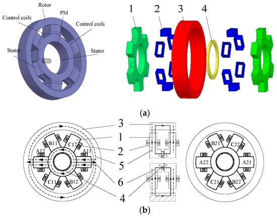
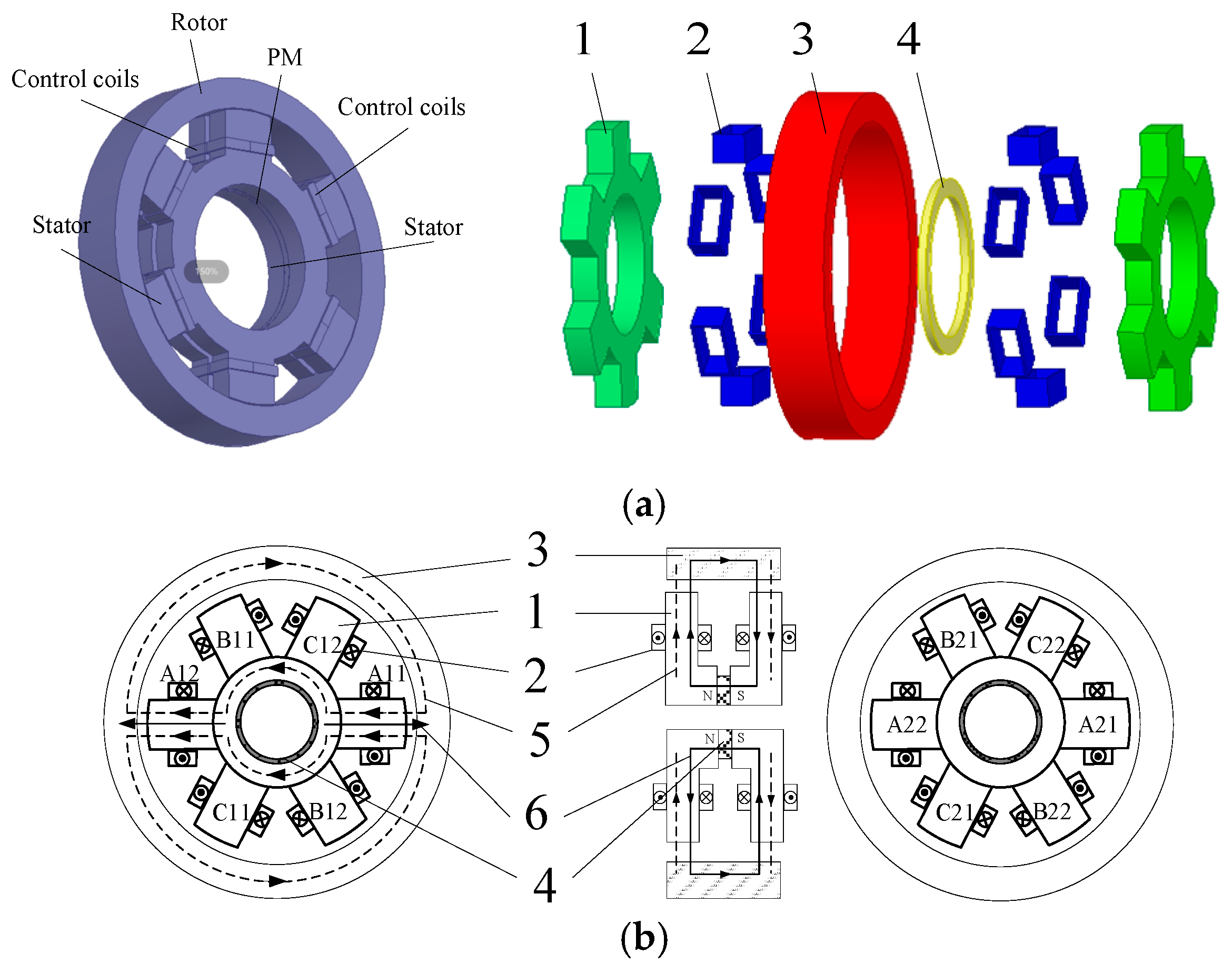
The model of the SHMB is shown in Figure 1. Figure 1a shows the explosive view of the SHMB, and different colors are used for each component of the SHMB.

Figure 1. Model of six-pole hybrid magnetic bearing. (a) Explosive view; (b) magnetic flux paths of (1) stator, (2) control coil, (3) rotor, (4) PM, (5) control magnetic circuit, and (6) permanent magnetic circuit.

There are two kinds of fluxes, bias flux and control flux in the SHMB. Depicted in Figure 1b, the bias flux is generated by the permanent magnet magnetizing along the z direction, and the specific flow direction is from the N pole of the permanent magnet, passing through the left radial stator, the left air gap, the rotor, the right air gap, and the right radial stator back to the other pole of the permanent magnet. The control flux is generated by the control coil of each pole and flows only in the side of the corresponding stator.

It can be seen in Figure 1 that the research object is a second-order system. The ADRC is outlined in the following section.

2.1. Tracking Differential

The system is as follows:

$$\left\{\begin{array}{l}{\dot{x}}_1=x_2\hfill \\ {\dot{x}}_2=u,\left|u\right|\le r\hfill \end{array}\right.$$

(1)

where x₁ is the current tracked position, x₂ is its derivative, u is the controlled quantity, and r is the accelerated speed.

The expression of “fast optimal control” in Formula (1) is:

$$\left\{\begin{array}{l}{\dot{x}}_1=x_2\hfill \\ {\dot{x}}_2=-r·\mathrm{sgn}(x_1+{\displaystyle \frac{x_2\left|x_2\right|}{2r}})\hfill \end{array}\right.$$

(2)

Substituting x₁(t) with x₁(t) − v(t) yields:

$$\left\{\begin{array}{l}{\dot{x}}_1=x_2\hfill \\ {\dot{x}}_2=-r·\mathrm{sgn}(x_1-v(t)+{\displaystyle \frac{x_2\left|x_2\right|}{2r}})\hfill \end{array}\right.$$

(3)

where v(t) is the input signal.

In the aforementioned equation, x₁(t) can track the system’s input signal v(t) at the maximum speed, and the derivative of v(t) can be expressed through the derivative of x₁(t) because of the performance of $-r·\mathrm{sgn}(x_1-v(t)+x_2\left|x_2\right|/2r)$. However, due to the inherent characteristics of the system, jitter may occur as the system stabilizes. The composite function fhan (x₁, x₂, r, h) is as follows:

$$\left\{\begin{array}{l}d=r{h}^2,a_0=h{x}_2\hfill \\ y=x_1+a_0\hfill \\ a_1=\sqrt{d(d+8\left|y\right|}\hfill \\ a_2=a_0+sign(y)(a_1-d)/2\hfill \\ s_y=(sign(y+d)-sign(y-d)/2\hfill \\ a=(a_0+y-a_2)s_y+a_2\hfill \\ s_a=(sign(a+d)-sign(a-d)/2\hfill \\ fhan=-r(a/d-sign(a))s_a-r·sign(a)\hfill \end{array}\right.$$

(4)

where h is the sampling step size and r is the velocity factor.

The TD of the system can be established according to this function.

$$\left\{\begin{array}{l}fh=fhan(x_1(k)-v(k),x_2(k),r,h)\hfill \\ x_1(k+1)=x_1(k)+h{x}_2(k)\hfill \\ x_2(k+1)=x_2(k)+h·fh\hfill \end{array}\right.$$

(5)

2.2. Expansion State Observer

For nonlinear systems:

$$\left\{\begin{array}{l}{\dot{x}}_1=x_2\\ {\dot{x}}_2=x_3+bu\\ {\dot{x}}_3=w(t)\end{array}\right.$$

(6)

And $x_3(t)=f(x_1(t),x_2(t))$; if ${\dot{x}}_3(t)=w(t)$ is recorded, then the system can be expanded into a new linear system:

$$\left\{\begin{array}{l}{\dot{x}}_1=x_2\hfill \\ {\dot{x}}_2=x_3+bu\hfill \\ {\dot{x}}_3=w(t)\hfill \\ y=x_1\hfill \end{array}\right.$$

(7)

We establish ESO for the expanded system as shown in Equation (7):

$$\left\{\begin{array}{l}{e}_1=z_1-y\hfill \\ {\dot{z}}_1=z_2-{\beta }_{01}{e}_1\hfill \\ {\dot{z}}_2=z_3-{\beta }_{02}fal(e,{\alpha }_1,\delta )+bu\hfill \\ {\dot{z}}_3=-{\beta }_{03}fal(e,{\alpha }_2,\delta )\hfill \end{array}\right.$$

(8)

where z₁, z₂, and z₃ denote the estimated values of x₁, x₂, and x₃; β₀₁, β₀₂, β₀₃ are three parameters of ESO; and δ denotes the filtering factor.

The corresponding discrete form of ESO is:

$$\left\{\begin{array}{l}e(k)=z_1(k)-y(k)\hfill \\ z_1(k+1)=z_1(k)+h\left[z_2(k)-{\beta }_{01}e(k)\right]\hfill \\ z_2(k+1)=z_2(k)+h\left[z_3(k)-{\beta }_{02}fal(e,{\alpha }_1,\delta )+bu\right]\hfill \\ z_3(k+1)=z_3(k)-h{\beta }_{03}fal(e,{\alpha }_2,\delta )\hfill \end{array}\right.$$

(9)

In the above formula:

$$fal(e,\alpha ,\delta )=\left\{\begin{array}{l}{\left|e\right|}^{\alpha }\mathrm{sgn}(e), \left|e\right|>\delta ;\hfill \\ e/{\delta }^{(1-\alpha )}, \left|e\right|\le \delta ; \hfill \end{array}\right.$$

(10)

When parameter b is known, z₁, z₂, and z₃ can effectively track the system’s state variables x₁, x₂, and x₃. The control input is defined as u = (u0(z₃(t))/b, and the controlled object Equation (6) becomes:

$$\left\{\begin{array}{l}{\dot{x}}_1=x_2\hfill \\ {\dot{x}}_2=f(x_1,x_2)-z_3(3)+bu\hfill \\ y=x_1\hfill \end{array}\right.$$

(11)

Furthermore, since the estimation error f(x₁(t), x₂(t)) − z₃(t) is close to zero, Equation (11) can be approximated as:

$$\left\{\begin{array}{l}{\dot{x}}_1=x_2\hfill \\ {\dot{x}}_2=bu\hfill \\ y=x_1\hfill \end{array}\right.$$

(12)

This achieves the tracking and compensation of the disturbance of the system by ESO, and the process from Equation (5) to Equation (12) is called dynamic compensation linearization.

2.3. Nonlinear Feedback Control Law

The nonlinear control combination constructed by the function fal is not only easy to implement but also exhibits excellent robustness and adaptability. For second-order controlled objects, the following form of NLSEF is adopted:

$$\left\{\begin{array}{l}{e}_1(k)=v_1(k)-z_1(k)\hfill \\ e_2(k)=v_2(k)-z_2(k)\hfill \\ u_0(k)={\beta }_{1}fal(e_1(k),{\alpha }_3,\delta )+{\beta }_{2}fal(e_2(k),{\alpha }_4,\delta )\hfill \\ u(k)=(u_0(k)-z_3(k))/b_0\hfill \end{array}\right.$$

(13)

where r is determined by the transition speed of TD and the system’s overall capacity; h denotes the sampling period; β₁ and β₂ function similarly to PD in the PID control; α₁ and α₂ typically range from 0 < α₁ < α₂ < 1; δ > 0 and is usually set as $5h\le \delta \le 10h$; and b should approximate the actual value or be substituted with the approximate value b₀.

β₀₁, β₀₂, and β₀₃ are three parameters of ESO, and the value of these three parameters affect the tracking and compensation of ESO, especially β₀₃, which can affect the tracking and compensation of z₃ on the total disturbance of the system. The MPSO is used to train β₀₁, β₀₂, and β₀₃ to get the optimal value.

3. Active Disturbance Rejection Control Based on Modified Particle Swarm Optimization

3.1. Modified Particle Swarm Optimization

The particle swarm optimization algorithm employs iterative updates to the position and velocity of each particle for spatial optimization. N_p is the population size; in a D-dimensional space, the position of the i particle can be expressed as $x_{i,t}=\left(x_{i,t}^1,x_{i,t}^2,x_{i,t}^3,\dots ,x_{i,t}^d\right)$; the speed can be expressed as $v_{i,t}=\left(v_{i,t}^1,v_{i,t}^2,v_{i,t}^3,\dots ,v_{i,t}^d\right)$; and the optimal position experienced is represented as $p_{i,t}=\left(p_{i,t}^1,p_{i,t}^2,p_{i,t}^3,\dots ,p_{i,t}^d\right)$, where 1 ≤ d ≤ D and t is the iteration number. The parameters of the i-th particle at the t-th iteration are as follows: $v_{i,t}$ is the i-th particle’s velocity and $x_{i,t}$ is the i-th particle’s position. At iteration t + 1, the particle swarm position and velocity update formulae are as follows:

$$\begin{array}{l}{v}_{i,t+1}^d={\omega }_{i,t}^d\times v_{i,t}^d+c_1\times rand\times \left(p_{i,t}^d-x_{i,t}^d\right)+c_2\times rand\times \left(p_{g,t}^d-x_{i,t}^d\right)\\ x_{i,t+1}^d=x_{i,t}^d+v_{i,t+1}^d\\ {\omega }_{i,t}^d=\left({\omega }_{\max }-{\omega }_k\times t\right)\times r+A_t\\ A_t\in \left\{0,0.1\right\}\end{array}$$

(14)

where $i=1,2,\dots ,N_p$ is the particle index; N_p is the population size; d is the d-dimensional space; t is the iteration count; c₁ and c₂ are learning factors; rand is a random number between 0 and 1; ${\omega }_{\max }$ is the maximum initial value of the inertia weight; ${\omega }_k$ is the slope of the inertia weight; A_t is the disturbance constant of the inertia weight, with a 15% probability of A_t being 0.1, otherwise A_t is 0; and r is a coefficient ranging from 0.8 to 1.2.

In the above formula, the inertia weight is multiplied by a coefficient r in the process of decreasing with 35% probability, and the random particles in the solution space are used to replace the particles obtained by the PSO with 25% probability.

By selecting ITAE as the fitness function J_ITAE:

$$J_{ITAE}={\displaystyle {\int }_0^{\infty }t|e(t)|\mathrm{d}t}$$

(15)

where e(t) denotes the system error.

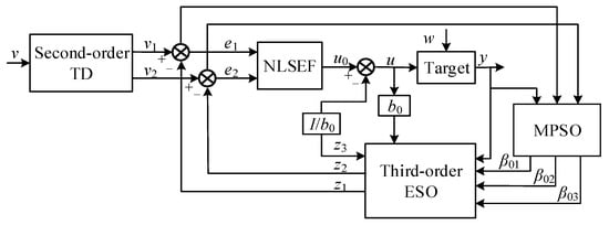
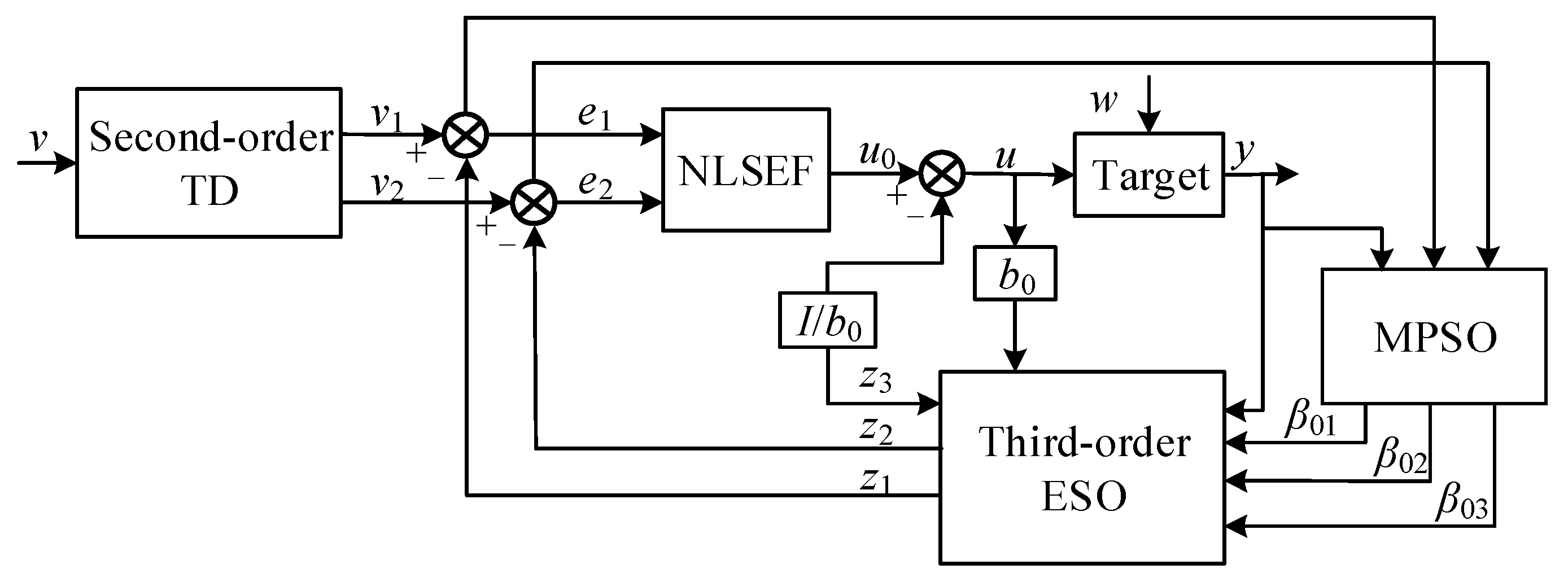
The three parameters (β₀₁, β₀₂, β₀₃) of the ADRC are obtained by training the MPSO. The structure of the ADRC based on the MPSO is shown in Figure 2.

Figure 2. The system structure block diagram of ADRC based on modified particle swarm optimization.

In Figure 2, v₁(t) and v₂(t) represent the tracking signal and differential signal respectively, which are generated by the system input v(t) through TD-based extraction of tracking and differential signals. z₁(t), z₂(t), and z₃(t) are the state variables estimated by the ESO, while w(t) denotes the exoteric interfere of the system.

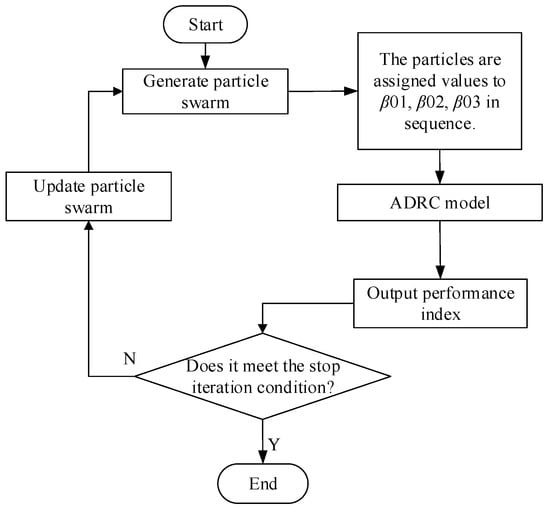
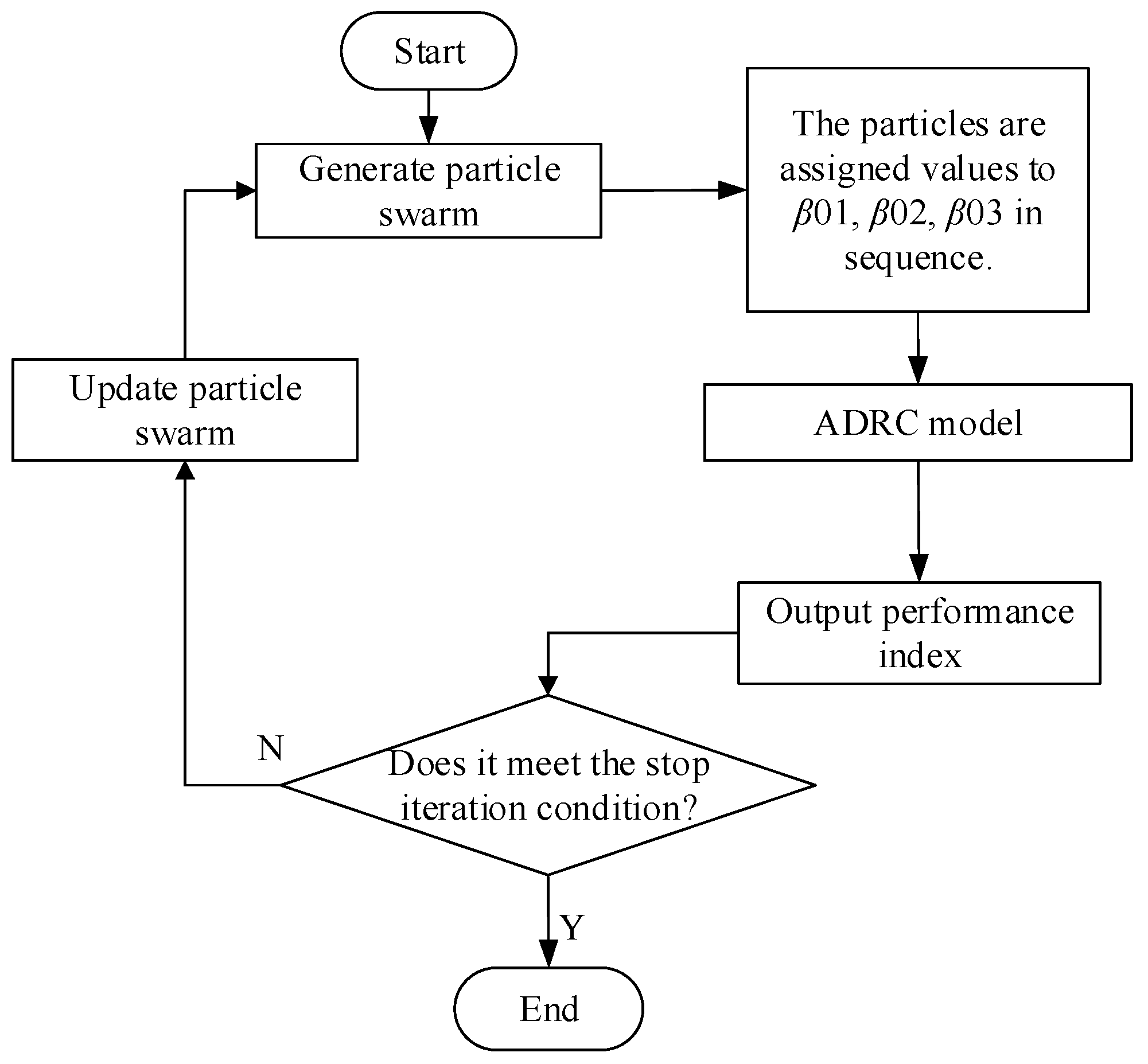
Figure 3 illustrates the flowchart for developing an ADRC based on an modified particle swarm optimization algorithm for SHMBs. The identification process is implemented online in real time, and the detailed process is as follows:

Figure 3. Flowchart of the ADRC based on the MPSO.

(a)

The MPSO algorithm is initialized: population size N_P = 50; maximum iteration of the algorithm T_max = 100; learning factors c₁ = c₂ = 2; initial maximum inertial weight ${\omega }_{\max }$ = 0.85; and the declining slope of the inertial weight coefficient ${\omega }_{\mathrm{k}}$ = 0.001. Particles are assigned to the parameters (β₀₁, β₀₂, β₀₃).

(b)

The parameters are input into the ADRC model, and the fitness function based on the MPSO is used to judge whether the ADRC model meets the expected effect.

(c)

The loop terminates when the fitness function criteria of the formula have met Formula (15), and the corresponding parameters are outputted. The position and velocity of the particle are updated according to (14) to obtain the next generation particle. Otherwise, the particle continues updating and repeats the above steps until the optimal performance parameters (β₀₁, β₀₂, β₀₃) are obtained, yielding the extended state observer. This completes one round of online identification.

(d)

In the next particle swarm optimization update cycle, the above steps are repeated to achieve online dynamic identification of the parameters.

3.2. Decoupling Control of SHMB

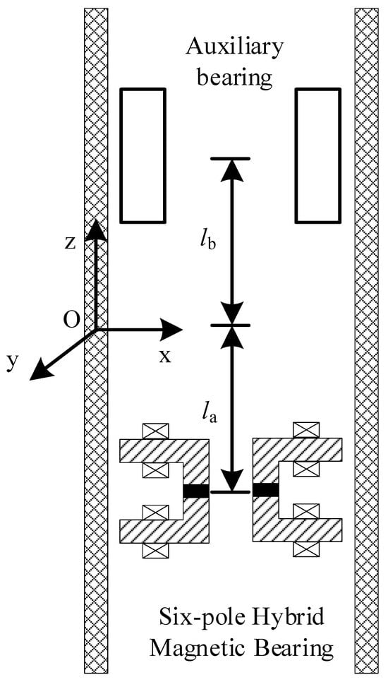
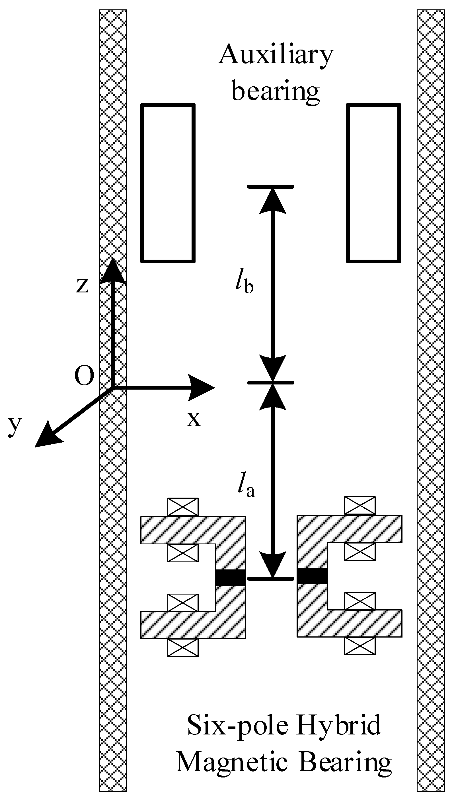
Figure 4 illustrates the force distribution on the SHMB. The rotor mass is denoted as m, with its center of mass as O. The mechanical angular velocity and moments of inertia about the z-axis are Ω and J_z, while the moments of inertia about the x- and y-axes are $J_x=J_y=J_{\mathrm{d}}$, where J_d is a constant. Based on rotor dynamics theory, the motion equations for the SHMB are derived as follows:

$$\left\{\begin{array}{l}m{\ddot{x}}_{\mathrm{o}}=F_x-f_x\\ m{\ddot{y}}_{\mathrm{o}}=F_y-f_y\\ J_x{\ddot{\theta }}_x=-l_{\mathrm{a}}(F_y-f_y)-J_z\Omega {\dot{\theta }}_y\\ J_y{\ddot{\theta }}_y=-l_{\mathrm{a}}(F_x-f_x)-J_z\Omega {\dot{\theta }}_x\end{array}\right.$$

(16)

Figure 4. Position diagram of each centroid of SHMBs.

Assuming the SHMB has offsets x and y in two directions, the variables in Figure 4 relate as follows:

$$\begin{array}{l}{x}_{\mathrm{o}}={\displaystyle \frac{l_b}{l_a+l_b}}x\\ y_{\mathrm{o}}={\displaystyle \frac{l_b}{l_a+l_b}}y\end{array}$$

(17)

By substituting (16) to (17), the expression yields:

$$\left\{\begin{array}{l}\ddot{x}=({\displaystyle \frac{1}{m}}+{\displaystyle \frac{l_a^2}{J_y}})F_x-{\displaystyle \frac{\Omega l_a{J}_z}{J_y(l_a+l_b)}}\dot{y}-({\displaystyle \frac{1}{m}}+{\displaystyle \frac{l_a^2}{J_y}})f_x\\ \ddot{y}=({\displaystyle \frac{1}{m}}+{\displaystyle \frac{l_a^2}{J_x}})F_y+{\displaystyle \frac{\Omega l_a{J}_z}{J_x(l_a+l_b)}}\dot{x}-({\displaystyle \frac{1}{m}}+{\displaystyle \frac{l_a^2}{J_x}})f_y\end{array}\right.$$

(18)

The mathematical model of the SHMB can be rewritten as follows:

$$\left\{\begin{array}{l}\ddot{x}=({\displaystyle \frac{1}{m}}+{\displaystyle \frac{l_{\mathrm{a}}^2}{J_{\mathrm{d}}}})k_{\mathrm{r}}x+{\displaystyle \frac{\Omega l_{\mathrm{a}}{J}_z}{J_x(l_{\mathrm{a}}+l_{\mathrm{b}})}}\dot{y}-({\displaystyle \frac{1}{m}}+{\displaystyle \frac{l_{\mathrm{a}}^2}{J_{\mathrm{d}}}})k_{i\mathrm{r}}{i}_x-({\displaystyle \frac{1}{m}}+{\displaystyle \frac{l_a^2}{J_y}})f_x\\ \ddot{y}=({\displaystyle \frac{1}{m}}+{\displaystyle \frac{l_{\mathrm{a}}^2}{J_{\mathrm{d}}}})k_{\mathrm{r}}y+{\displaystyle \frac{\Omega l_{\mathrm{a}}{J}_z}{J_x(l_{\mathrm{a}}+l_{\mathrm{b}})}}\dot{x}-({\displaystyle \frac{1}{m}}+{\displaystyle \frac{l_{\mathrm{a}}^2}{J_{\mathrm{d}}}})k_{i\mathrm{r}}{i}_y-({\displaystyle \frac{1}{m}}+{\displaystyle \frac{l_a^2}{J_x}})f_y\end{array}\right.$$

(19)

System state variables are selected as:

$$X={\left[x_1, x_2, x_3, x_4\right]}^{\mathrm{T}}={\left[x, y, \dot{x}, \dot{y}\right]}^{\mathrm{T}}$$

(20)

Variables can be entered as:

$$U={\left[u_1, u_2\right]}^{\mathrm{T}}={\left[i_x, i_y\right]}^{\mathrm{T}}$$

(21)

The output variable is:

$$Y={\left[ y_1, y_2\right]}^{\mathrm{T}}={\left[x, y\right]}^{\mathrm{T}}$$

(22)

The state equation of the SHMB is obtained as follows:

$$\left\{\begin{array}{l}{\dot{x}}_1=\dot{x}\\ {\dot{x}}_2=\dot{y}\\ {\dot{x}}_3=({\displaystyle \frac{1}{m}}-{\displaystyle \frac{l_{\mathrm{a}}^2}{J_{\mathrm{d}}}})k_{\mathrm{r}}{x}_1+{\displaystyle \frac{\Omega l_{\mathrm{a}}{J}_z}{J_x(l_{\mathrm{a}}+l_{\mathrm{b}})}}{x}_4-({\displaystyle \frac{1}{m}}-{\displaystyle \frac{l_{\mathrm{a}}^2}{J_{\mathrm{d}}}})k_{i\mathrm{r}}{u}_1-({\displaystyle \frac{1}{m}}+{\displaystyle \frac{l_a^2}{J_y}})f_x\\ {\dot{x}}_4=({\displaystyle \frac{1}{m}}-{\displaystyle \frac{l_{\mathrm{a}}^2}{J_{\mathrm{d}}}})k_{\mathrm{r}}{x}_2+{\displaystyle \frac{\Omega l_{\mathrm{a}}{J}_z}{J_x(l_{\mathrm{a}}+l_{\mathrm{b}})}}{x}_3-({\displaystyle \frac{1}{m}}-{\displaystyle \frac{l_{\mathrm{a}}^2}{J_{\mathrm{d}}}})k_{i\mathrm{r}}{u}_2-({\displaystyle \frac{1}{m}}+{\displaystyle \frac{l_a^2}{J_x}})f_y\end{array}\right.$$

(23)

It can be rewritten as follows:

$$\left\{\begin{array}{l}\ddot{x}=k_{11}{i}_x+k_{12}x+k_{13}\dot{y}+k_{14}\\ \ddot{y}=k_{21}{i}_y+k_{22}y+k_{23}\dot{x}+k_{24}\end{array}\right.$$

(24)

where k_ij (i, j = 1, 2, 3, 4) denotes the coefficients.

This can be expressed as:

$$\left\{\begin{array}{l}{w}_x=k_{13}\dot{y}+k_{14}\\ w_y=k_{23}\dot{x}+k_{24}\end{array}\right.$$

(25)

Substituting (25) to (24) yields the expression:

$$\left\{\begin{array}{l}\ddot{x}=k_{11}{i}_x+k_{12}x+w_x\\ \ddot{y}=k_{21}{i}_y+k_{22}y+w_y\end{array}\right.$$

(26)

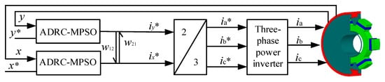
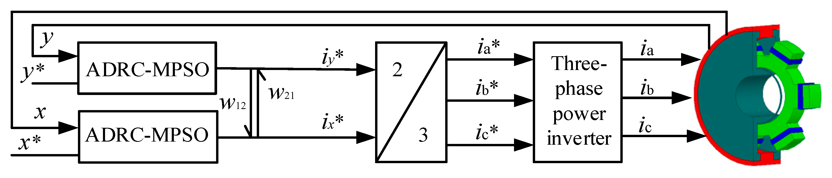
The decoupling of two radial degrees of freedom in a six-pole outer rotor radial hybrid magnetic bearing is achieved using a modified particle swarm optimization (MPSO)-based ADRC. The ESO (electrostatic stabilization oscillator) performs real-time estimation and compensation for the corresponding w_i (i = x,y), transforming the six-pole radial hybrid magnetic bearing system into a two-input (i_x,i_y) and two-output (x,y) uncoupled second-order linear system. Each radial degree of freedom is controlled by a modified PSO-based ADRC, with both controllers sharing identical structures and algorithms. ESO compensates for internal and external disturbances. The decoupling control block diagram of the six-pole radial hybrid magnetic bearing’s modified PSO-based ADRC is shown in Figure 5.

Figure 5. Block diagram of ADRC-MPSO for SHMBs.

The displacement signals x and y of the rotor, along with the given displacement signal x* and y*, are processed by the ADRC-MPSO using displacement sensors. Two expected currents i_x* and i_y* in different directions are obtained, the expected currents i_x* and i_y* in the x and y directions are transformed via a 2/3 conversion into the expected currents for phases A, B, and C, which are i_a* i_b* i_c*. These three-phase expected currents are then converted by a three-phase inverter into three-phase control currents i_a i_b i_c to regulate the rotor radial displacement. In the diagram, w₁₂ and w₂₁ represent coupling between different degrees of freedom.

4. Simulation Analysis of Decoupling Control for SHMB

MPSO is used to train parameters for an ADRC, yielding optimal parameters for its extended state observer. The ADRC-MPSO is implemented alongside a PID controller and a conventional ADRC for comparison. The conventional ADRC parameters include: extended state observer parameters β₀₁ = 30,000, β₀₂ = 300,000, β₀₃ = 5000, b₀ = 0.4, α₁ = 0.6, α₂ = 0.4, and δ = 0.002; nonlinear feedback control parameters β₁ = 40, β₂ = 0.01, δ = 0.002, α₃ = 0.6, and α₄ = 0.8; and tracking differentiator parameters (h = 0.02, r = 250). The parameters of the PID controller are k_P = 2, k_I = 0.0004, and k_D = 0.001. The parameters of the ADRC-MPSO are largely identical to the conventional version, with only β₀₁, β₀₂, and β₀₃ optimized through MPSO. The MPSO algorithm is configured with 100 iterations t, a population size of 50 generations N_p, learning factors c₁ and c₂ are set to 2, and an initial inertia weight of 0.85. Simulation experiments are conducted to compare the ADRC-MPSO with both the PID controller and the conventional ADRC.

4.1. Simulation of Six-Pole Hybrid Magnetic Bearing Under Different Disturbance Signals

A simulation comparison of the ADRC-MPSO and PID controller is carried out under different disturbance conditions. The quantitative performance indices summary table is shown in Table 1.

Table 1. The quantitative performance indices summary table.

Performance Indices	Value
Peak displacement of ADRC-MPSO/mm	0.12
Peak displacement of PID/mm	0.08
Settling time of ADRC-MPSO/s	0.04
Settling time of PID/s	0.018
Frequency of the sinusoidal disturbance/Hz	100
Biggest fluctuation of PID/mm	0.13
Biggest fluctuation of ADRC-MPSO/mm	0.05
Mean value of noise disturbance	0
Variance of noise disturbance	0.01
Sampling time of noise disturbance/ms	1

4.1.1. Step Disturbance Simulation

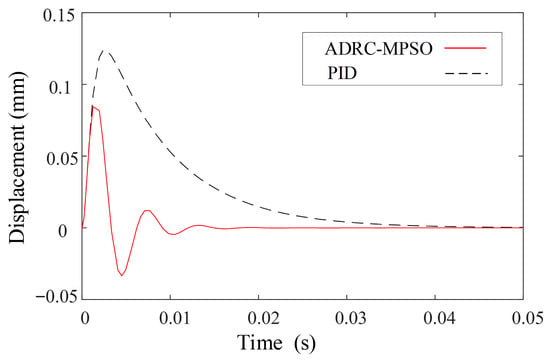
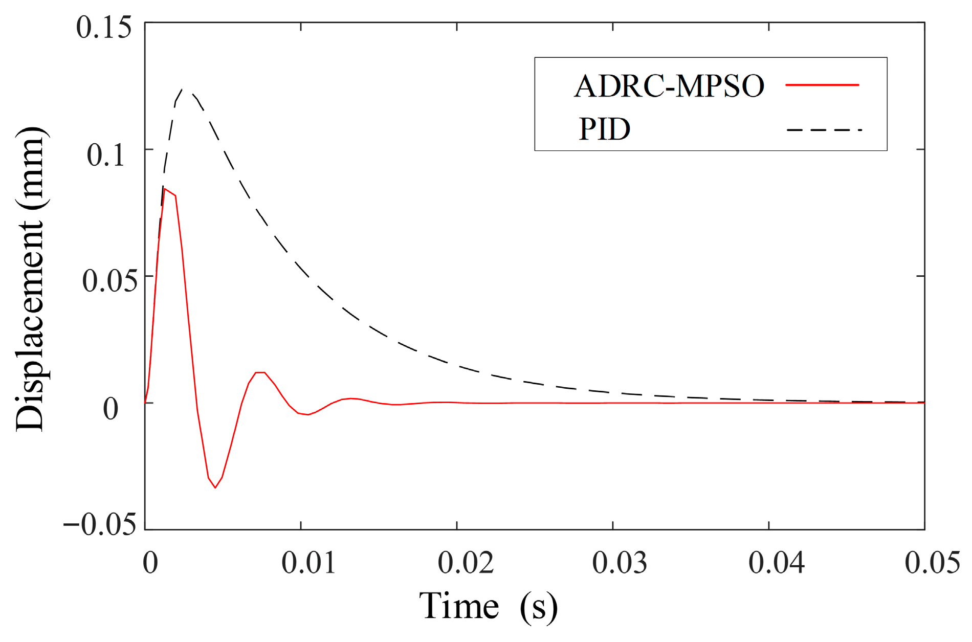
When magnetic bearings experience load variations during stable suspension, significant waveform changes occur. To observe rotor displacement changes during simulations, a step signal was introduced. Figure 6 displays the simulation waveform of rotor displacement with step disturbance. The figure reveals that the PID controller’s maximum displacement fluctuation is 0.12 mm, with a recovery time of 0.04 s from initial fluctuation to equilibrium position. In contrast, the ADRC-MPSO achieves a maximum displacement fluctuation of 0.08 mm, with a recovery time of 0.018 s. This demonstrates that the ADRC-MPSO exhibits smaller displacement fluctuations, faster equilibrium recovery, and enhanced disturbance resistance when subjected to load variations.

Figure 6. Waveforms of phase step perturbation simulations.

4.1.2. Simulation of Sinusoidal Disturbance

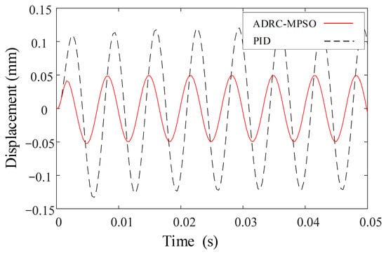
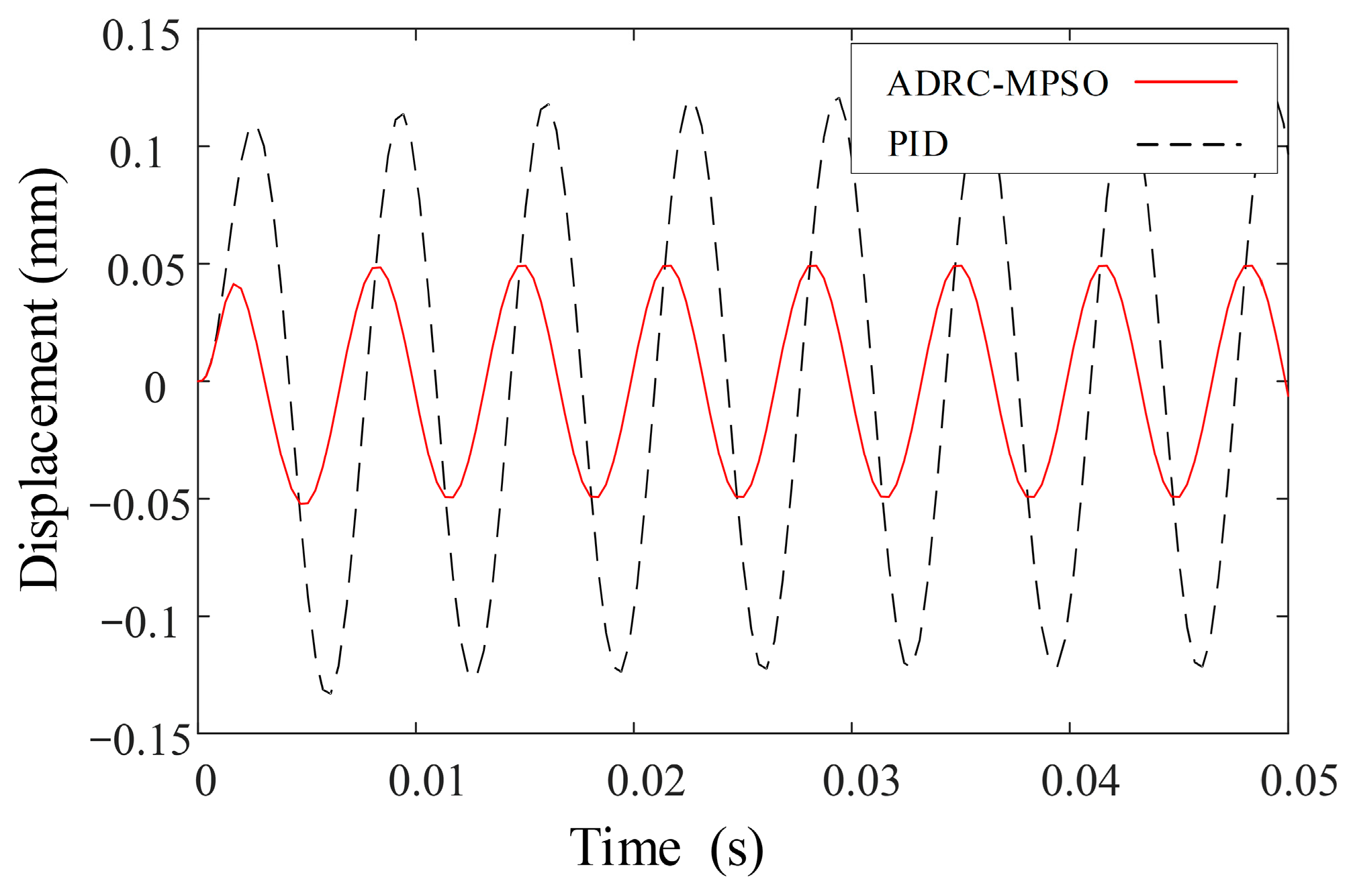
When a magnetic bearing experiences sinusoidal disturbance during stable suspension, its waveform undergoes changes. To observe rotor displacement variations during simulation, a sinusoidal signal was introduced. Figure 7 presents the simulation waveform of the magnetic bearing rotor under sinusoidal disturbance. The figure demonstrates that the biggest fluctuation of the PID controller reaches 0.13 mm, whereas the ADRC-MPSO achieves a maximum fluctuation of 0.05 mm. This indicates that the magnetic bearing rotor controlled by the ADRC-MPSO exhibits significantly smaller displacement fluctuations and stronger disturbance resistance under sinusoidal interference conditions compared to the PID controller.

Figure 7. Waveforms of sinusoidal perturbation simulations.

4.1.3. Noise Disturbance Simulation

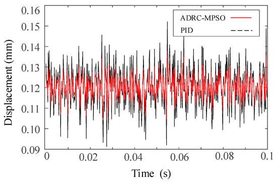
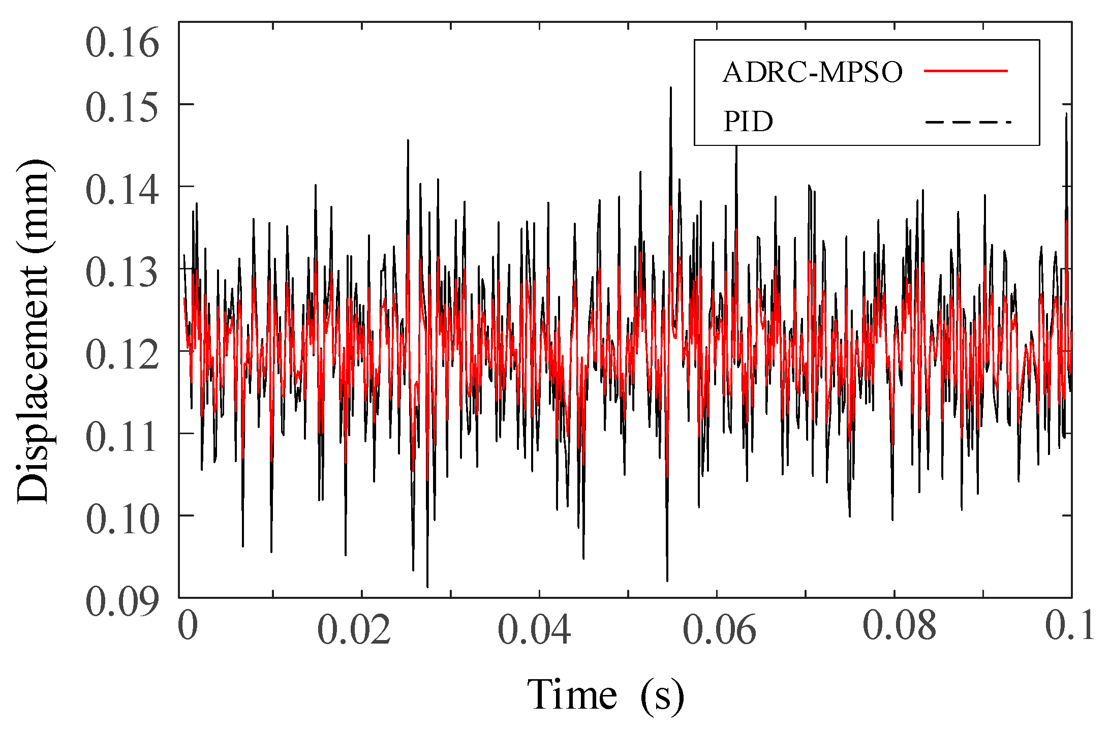
When a magnetic bearing experiences noise disturbance during stable suspension, its waveform undergoes changes. Therefore, noise disturbance is introduced in simulations to observe rotor displacement variations. Figure 8 presents the simulation waveform under noise disturbance. The comparison demonstrates that the rotor of the SHMB controlled by the ADRC-MPSO exhibits significantly smaller displacement fluctuations and stronger disturbance resistance under noise interference conditions compared to the PID controller.

Figure 8. Waveforms of noise perturbation simulations.

4.2. Suspension Simulation of Six-Pole Hybrid Magnetic Bearing

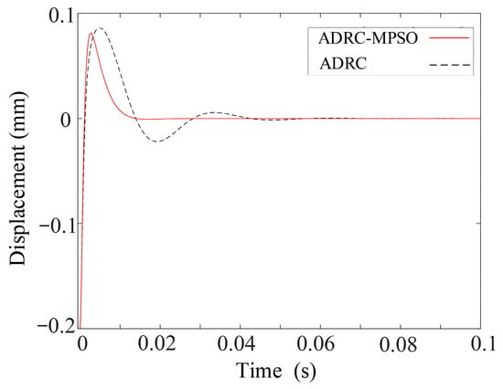
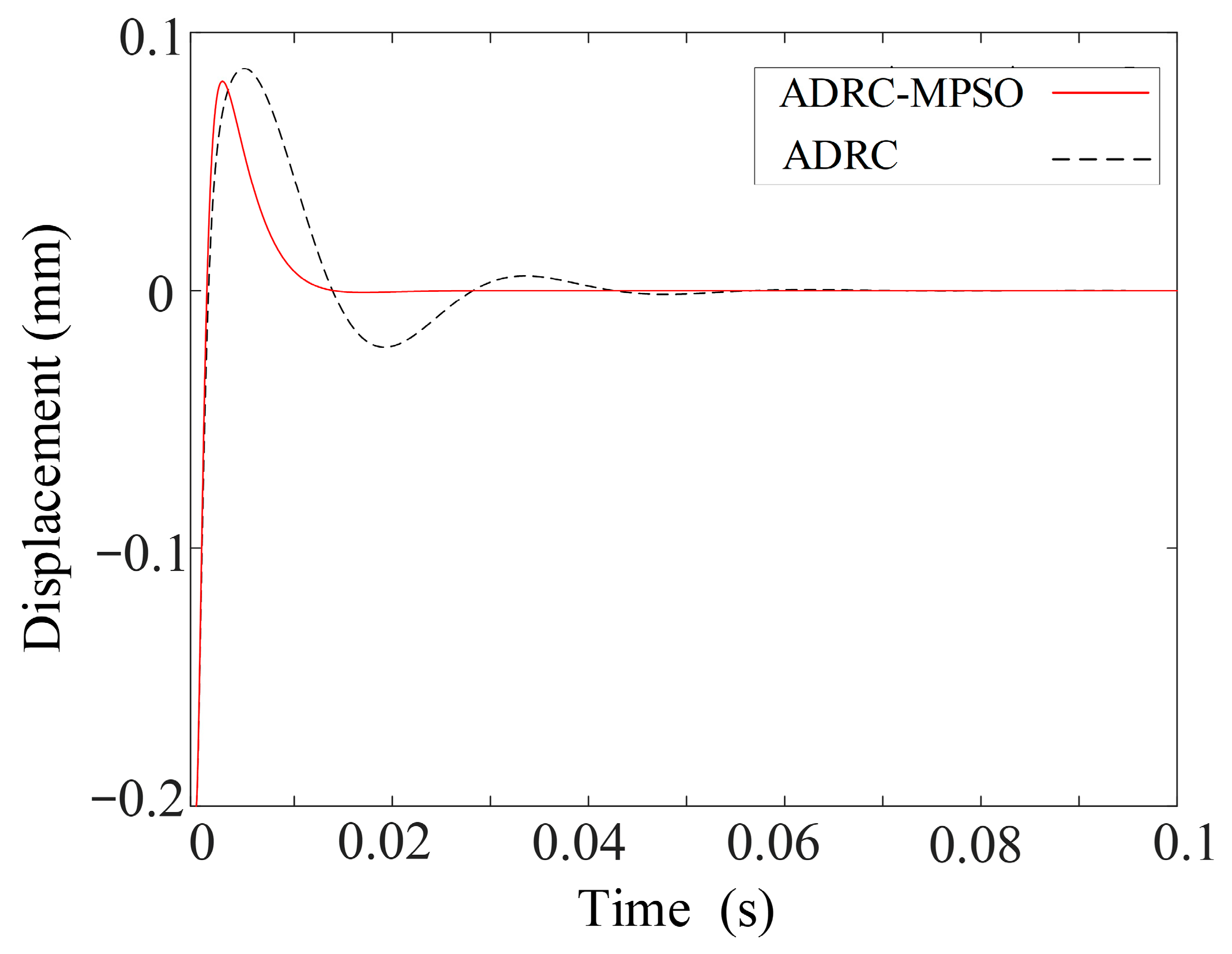
Figure 9 displays the waveform of a rotor’s levitation process from rest. The rotor’s initial position is (0 mm, −0.2 mm). The ADRC achieves equilibrium at 0.012 s post levitation with a 0.07 mm overshoot, whereas the traditional controller reaches equilibrium at 0.05 s with 0.08 mm overshoot. Thus, the ADRC-MPSO demonstrates a shorter response time and superior stability.

Figure 9. Rotor floating simulations of ADRC under different algorithms.

4.3. Simulation of Anti-Interference of SHMB

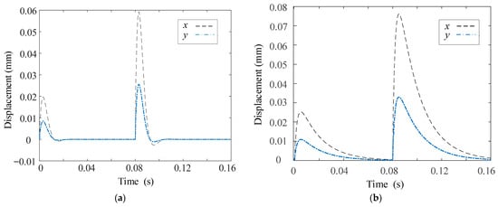
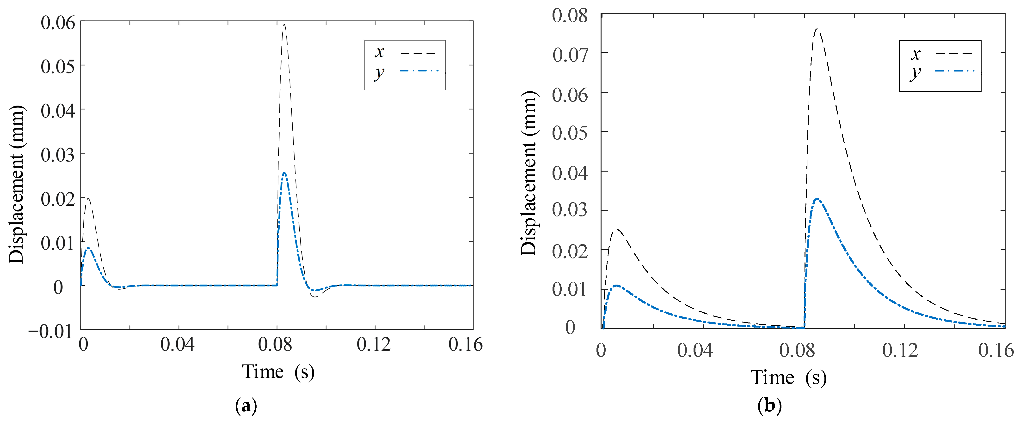
Figure 10a shows the displacement curves in various directions of the ADRC-MPSO under external disturbances. A 100 N external disturbance is applied to the x direction at time 0 s, making the displacement in the x direction 0.02 mm and in the y direction 0.008 mm. At time 0.08 s, a 200 N disturbance is applied to the x direction, making the displacement in the x direction 0.059 mm and in the y direction 0.025 mm. Figure 10b displays the displacement curves of a conventional ADRC under external disturbances. The same parameters are applied. A 100 N disturbance at time 0 s produces x direction displacement of 0.025 mm and y direction displacement of 0.012 mm. At time 0.08 s, a 200 N disturbance causes x direction displacement of 0.077 mm and y direction displacement of 0.033 mm. By comparing the ADRC-MPSO and the traditional ADRC under the external disturbance, it was found that the ADRC-MPSO has better anti-disturbance ability than the traditional ADRC under the different external disturbance.

Figure 10. Simulations of ADRC under different algorithms when the rotor is disturbed. (a) ADRC based on modified particle swarm optimization; (b) ADRC.

5. Prototype and Experiment

5.1. Experimental Prototype and Parameters

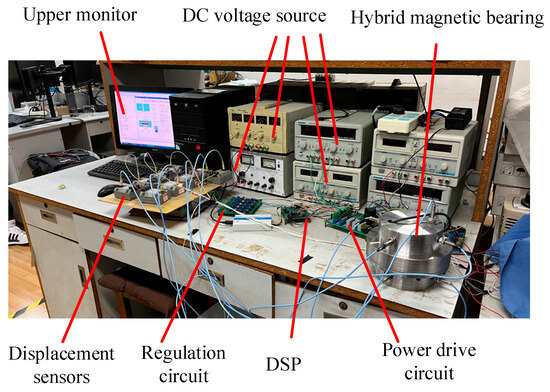
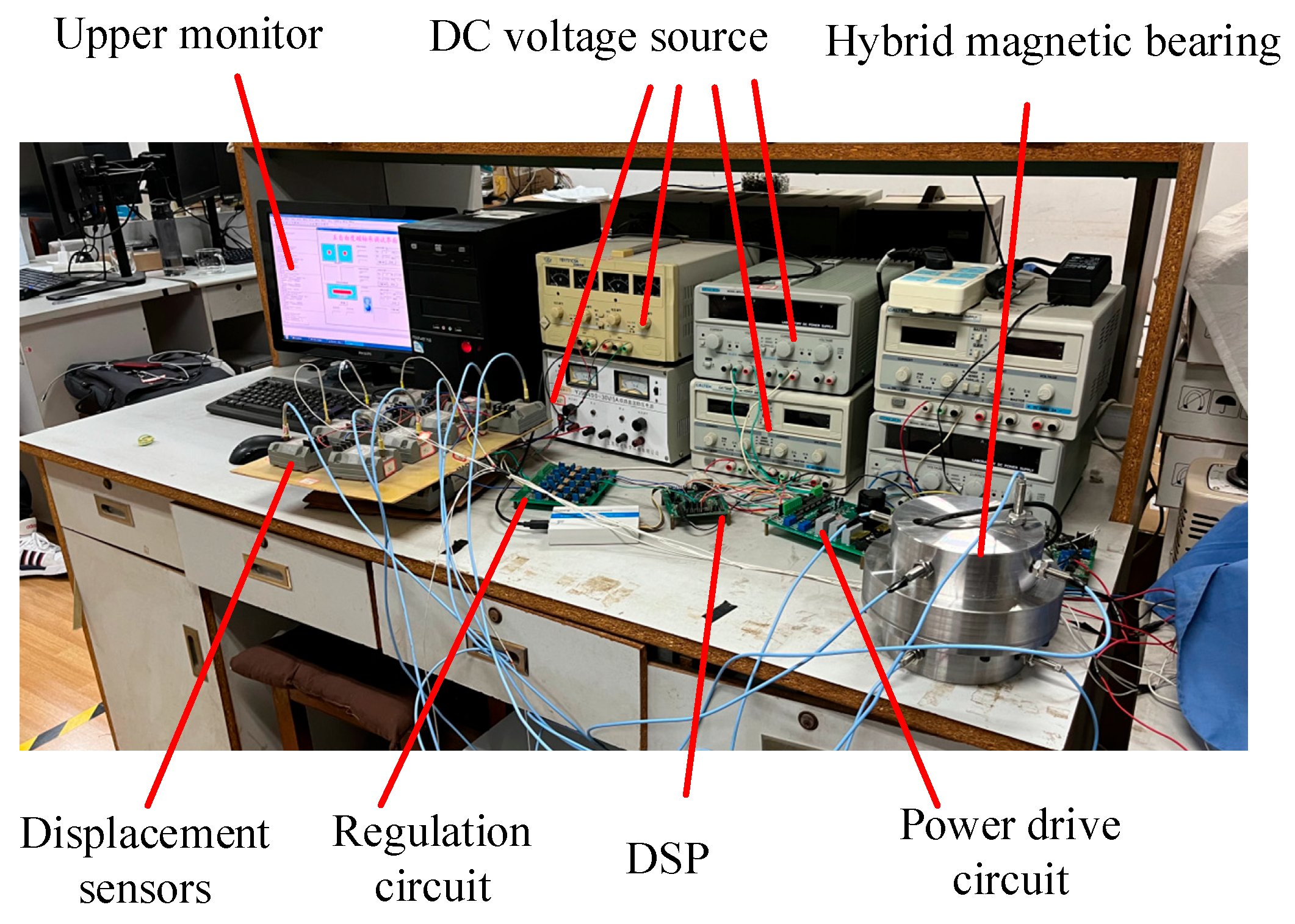
In order to verify the accuracy of the above analysis results and further analyze the performance of the six-pole hybrid magnetic bearing, an experimental platform is designed and manufactured as shown in Figure 11. The experimental platform mainly comprises an eddy current displacement sensor, displacement signal interface circuit, DC power supply, radial power drive board, AC power supply, PC machine, and DSP controller.

Figure 11. Experimental platform.

According to the design requirements of the SHMB, the key parameters of SHMB are designed. The design variables are shown in Table 2.

Table 2. Design variables.

Parameter	Value
Outer diameter of stator yoke/mm	82
Inner diameter of stator yoke/mm	54
Axial length of stator/mm	10
Length of air gap/mm	0.5
Magnetic pole area/mm2	288
Outer diameter of rotor/mm	142
Inner diameter of rotor/mm	118
Axial length of rotor/mm	23
Coil turns	160
Outer diameter of PM/mm	72
Inner diameter of PM/mm	58
Axial length of PM/mm	3
Magnetic pole width/mm	24
Magnetic pole angle/°	31
Extreme boot thickness/mm	4
Magnetic pole root width/mm	16

5.2. Suspension Experiments of Six-Pole Hybrid Magnetic Bearing

5.2.1. Floating Experiment

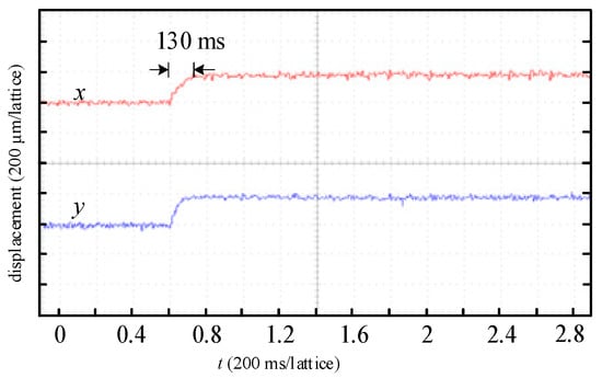
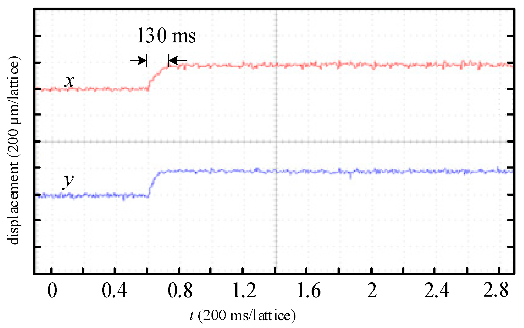
Figure 12 shows the waveform of the SHMB rotor during its transition from stationary to levitation. The x-axis represents time, while the y-axis indicates the rotor’s displacement in both x and y directions. The graph demonstrates that the rotor achieves levitation after 130 ms, stabilizing at equilibrium, and subsequently remains in this balanced state without further movement.

Figure 12. The waveform of rotor floatation.

5.2.2. Anti-Disturbance Experiment

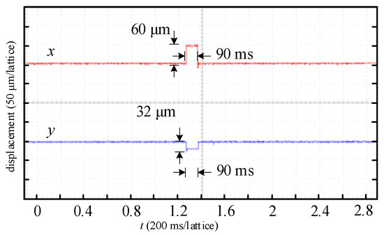
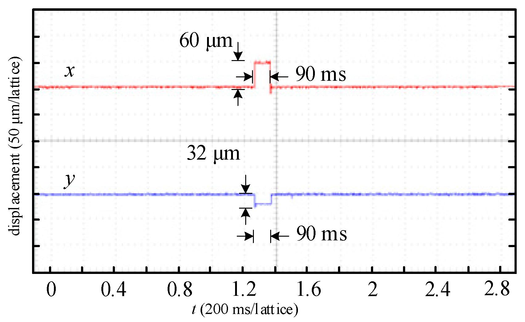
Figure 13 displays the waveform of the SHMB under disturbance. The x-axis represents time, while the y-axis shows the rotor’s displacement in both x and y directions. Initially, the rotor is at 0 μm in both x and y directions. At 1.24 s, a 200 N external disturbance force is applied, causing the rotor to vibrate. The displacement in the x direction reaches 60 μm and returns to equilibrium within 90 ms, while the y direction displacement reaches 32 μm and also returns to equilibrium within 90 ms.

Figure 13. The waveform of rotor disturbance.

5.2.3. Load Experiment

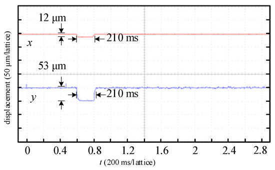
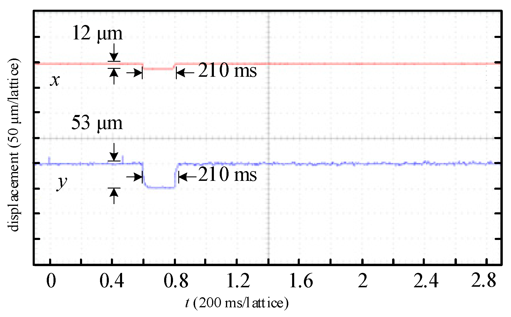
Figure 14 presents the experimental waveform of radial load on the SHMB. The x-axis represents time, while the y-axis shows the rotor’s displacement in both x and y directions. Initially, the rotor is in equilibrium. At 0.6 s, a 200 N load is applied to the y direction, causing the rotor to deviate from equilibrium. After 210 ms, the rotor returns to equilibrium with a 12 μm displacement in the negative x direction and 53 μm displacement in the negative y direction.

Figure 14. The experiment results of adding load.

6. Conclusions

In this paper, the ADRC-MPSO was put forward, which solved the coupling problem of SHMBs. The particle swarm algorithm was modified, where the inertia weight of the PSO was multiplied by a coefficient r in the process of decreasing with 35% probability, and the random particles in the solution space were used to replace the particles obtained by the particle swarm algorithm with 25% probability. The modified particle swarm algorithm was used to train β₀₁, β₀₂, and β₀₃ to get the optimal value.

Under different disturbance signals, the simulation results of ADRC-MPSO had better anti-interference performance than that of PID, the floating simulation of the ADRC-MPSO demonstrated a shorter response time and superior stability than the ADRC. The anti-interference simulation of the ADRC-MPSO had better anti-disturbance ability than the traditional ADRC under the different external disturbance.

An experimental platform was designed: the floating experiment showed the rotor could regain its equilibrium position in a very short time; and the anti-disturbance experiment and the load experiment showed SHMBs had better stability and better anti-disturbance ability. The experimental results show that the ADRC-MPSO has good performance.

References

- Zhou, M.Q.; Shuai, Y.X.; Jiang, D.; Liu, Z.C. Active Magnetic Bearing PID Tuning with Model-Free Time-Domain Analysis Based Heuristic Algorithm. IEEE Trans. Ind. Inform. 2024, 20, 12157–12167. [Google Scholar] [CrossRef] [Scilit]
- Wang, T.; Zhang, W.Y. Review on Key Development of Magnetic Bearings. Machines 2025, 13, 113. [Google Scholar] [CrossRef] [Scilit]
- Zhang, W.Y.; Zhu, H.Q.; Yang, Z.B.; Sun, X.D.; Yuan, Y. Nonlinear Model Analysis and “Switching Model” of AC–DC Three Degree of Freedom Hybrid Magnetic Bearing. IEEE/ASME Trans. Mechatron. 2016, 21, 1102–1115. [Google Scholar] [CrossRef] [Scilit]
- Liu, Y.J.; Xiong, H.J.; Zhang, H. Research on Active Disturbance Rejection Control of Active Magnetic Bearing-Rotor System. In Proceedings of the 2021 6th Asia Conference on Power and Electrical Engineering (ACPEE), Chongqing, China, 8–11 April 2021; pp. 873–877. [Google Scholar]
- Liu, H.Q.; Ye, C.Y.; Wang, T.Y.; Zhao, Y.F. New Sliding Mode Control Algorithm of Magnetic Bearing Based on State Feedback Decoupling. In Proceedings of the 2024 IEEE China International Youth Conference on Electrical Engineering (CIYCEE), Wuhan, China, 6–8 November 2024; pp. 1–7. [Google Scholar]
- Le, Q.Y.; Zhu, W.G. Electromagnetic Performance Analysis on the Novel Radial and Axial Hybrid Magnetic Bearing. In Proceedings of the 2020 IEEE International Conference on Applied Superconductivity and Electromagnetic Devices (ASEMD), Tianjin, China, 16–18 October 2020; pp. 1–2. [Google Scholar]
- Sun, J.Z.; Ma, T.C. Inverse Decoupling Control of Active Electromagnetic Bearing System. In Proceedings of the 2024 3rd International Conference on Energy and Electrical Power Systems (ICEEPS), Guangzhou, China, 14–16 July 2024; pp. 1350–1354. [Google Scholar]
- Wang, S.S.; Zhu, H.Q.; Wu, M.Y.; Zhang, W.Y. Active Disturbance Rejection Decoupling Control for Three-Degree-of-Freedom Six-Pole Active Magnetic Bearing Based on BP Neural Network. IEEE Trans. Appl. Supercond. 2020, 30, 3603505. [Google Scholar] [CrossRef] [Scilit]
- Ma, Z.H.; Zhu, H.Q. Decoupling Control of Six-Pole Radial Active Magnetic Bearings Based on BP Neural Network Inverse Optimized by Improved Mind Evolutionary Algorithm. IEEE Trans. Power Electron. 2026, 41, 1841–1852. [Google Scholar] [CrossRef] [Scilit]
- Zhang, J.; Zhu, H.Q. Decoupling Control of Six-Pole Radial Hybrid Magnetic Bearing Based on Least Square Support Vector Machine Inverse System. IEEE J. Emerg. Sel. Top. Power Electron. 2024, 12, 607–617. [Google Scholar] [CrossRef] [Scilit]
- Li, H.M.; Zhu, H.Q.; Ju, J.T. Neural Network Inverse System Decoupling Control for Six-Pole Radial-Axial Hybrid Magnetic Bearing Based on Deep Fuzzy Inference. IEEE Trans. Power Electron. 2026, 41, 5067–5076. [Google Scholar] [CrossRef] [Scilit]
- Liu, G.; Zhu, H.Q.; Wu, M.Y.; Zhang, W.Y. Principle and Performance Analysis for Heterpolar Permanent Magnet Biased Radial Hybrid Magnetic Bearing. IEEE Trans. Appl. Supercond. 2020, 30, 3602704. [Google Scholar] [CrossRef] [Scilit]
- Jiang, H.; Su, H.Z.; Wang, D. Analytical Calculation of Active Magnetic Bearing Based on Distributed Magnetic Circuit Method. IEEE Trans. Energy Convers. 2021, 36, 1841–1851. [Google Scholar] [CrossRef] [Scilit]
- Wang, D.; Le, Y.; Han, X.; Zheng, S. Calculation and Analysis of an Integrated Motor-Magnetic Bearing Magnetic Circuit Model. IEEE Trans. Ind. Electron. 2025, 72, 876–886. [Google Scholar] [CrossRef] [Scilit]
- Zhong, Y.L.; Wu, L.J.; Huang, X.Y.; Fang, Y.T.; Zhang, J. An Improved Magnetic Circuit Model of a 3-DOF Magnetic Bearing Considering Leakage and Cross-Coupling Effects. IEEE Trans. Magn. 2017, 53, 8002506. [Google Scholar] [CrossRef] [Scilit]
- Zhang, T.; Wang, Z.X. Structure and Levitation Force Characteristics Analysis for Novel Radial Hybrid Magnetic Bearing. IEEE Trans. Appl. Supercond. 2021, 31, 0602705. [Google Scholar] [CrossRef] [Scilit]
- Li, W.Y.; Hu, J.H.; Su, Z.Z.; Wang, D. Radial Displacement Detection Using Sensing Coils Weakly Coupled with Magnetic Bearing. IEEE Sens. J. 2022, 22, 20352–20359. [Google Scholar] [CrossRef] [Scilit]
- Wang, K.; Wang, D.; Shen, Y.; Zhang, X.B.; Chen, J.Q.; Zhang, Y. Subdomain Method for Permanent Magnet Biased Homo-Polar Radial Magnetic Bearing. IEEE Trans. Magn. 2016, 52, 8300405. [Google Scholar] [CrossRef] [Scilit]
- Jiang, H.; Su, Z.Z.; Wang, D.; Wu, C. Multiparameter Identification for Active Magnetic Bearing with Uncertainties Based on a Coupled Nonlinear Model. IEEE Trans. Ind. Electron. 2023, 70, 10431–10441. [Google Scholar] [CrossRef] [Scilit]
- Di, C.; Petrov, I.; Pyrhönen, J.J.; Bao, X.H. Unbalanced Magnetic Pull Compensation With Active Magnetic Bearings in a 2 MW High-Speed Induction Machine by FEM. IEEE Trans. Magn. 2018, 54, 8202913. [Google Scholar] [CrossRef] [Scilit]
- Liu, Z.Y.; Cao, X.; Cai, J. A Magnetic Bearing Switched Reluctance Motor With Simultaneous Excitation by a Modified Half-Bridge Converter. IEEE Trans. Magn. 2019, 55, 7500905. [Google Scholar] [CrossRef] [Scilit]
- Noshadi, A.; Shi, J.; Lee, W.S.; Shi, P.; Kalam, A. System Identification and Robust Control of Multi-Input Multi-Output Active Magnetic Bearing Systems. IEEE Trans. Control Syst. Technol. 2016, 24, 1227–1239. [Google Scholar] [CrossRef] [Scilit]
- Wang, H.; Wu, Z.G.; Liu, K.; Wei, J.B.; Hu, H.J. Modeling and Control Strategies of a Novel Axial Hybrid Magnetic Bearing for Flywheel Energy Storage System. IEEE/ASME Trans. Mechatron. 2022, 27, 3819–3829. [Google Scholar] [CrossRef] [Scilit]
- Gong, Z.; Desenfans, P.; Pissoort, D.; Hallez, H.; Vanoost, D. Multiphysics Coupling Model to Characterise the Behaviour of Induction Motors with Eccentricity and Bearing Faults. IEEE Trans. Energy Convers. 2024, 39, 146–159. [Google Scholar] [CrossRef] [Scilit]
- Jiang, Y.; Ma, X.; Fan, Y. Rotor Displacement Self-Sensing Approach for Permanent Magnet Biased Magnetic Bearings Using Double-Axis PWM Demodulation. IEEE Sens. J. 2018, 18, 7932–7940. [Google Scholar] [CrossRef] [Scilit]
- Tan, D.; Lu, C. The Influence of the Magnetic Force Generated by the In-Wheel Motor on the Vertical and Lateral Coupling Dynamics of Electric Vehicles. IEEE Trans. Veh. Technol. 2016, 65, 4655–4668. [Google Scholar] [CrossRef] [Scilit]
- Nie, Z.; Chen, Z.Y.; Yan, W.; Xia, S.; Yu, Y.; Zou, G.; Liu, F.; Zhong, Y.; Fang, J.; Zhou, X.; et al. Optimization of Rail-Armature Coupling for the Enhanced Electromagnetic Pellet Injection in J-TEXT Tokamak. IEEE Trans. Plasma Sci. 2024, 52, 3326–3334. [Google Scholar] [CrossRef] [Scilit]
Disclaimer/Publisher’s Note: The statements, opinions and data contained in all publications are solely those of the individual author(s) and contributor(s) and not of MDPI and/or the editor(s). MDPI and/or the editor(s) disclaim responsibility for any injury to people or property resulting from any ideas, methods, instructions or products referred to in the content. |
© 2026 by the authors. Licensee MDPI, Basel, Switzerland. This article is an open access article distributed under the terms and conditions of the Creative Commons Attribution (CC BY) license.