


Abstract
This study develops and evaluates three complementary predictive modeling frameworks for gearbox oil temperature forecasting: Stochastic Differential Equation (SDE) modeling with iterative Markov correction, multi-objective genetic algorithm-enhanced grey modeling (MOGA-GM(1,N)), and multi-output Gaussian Process Regression (MO-GPR). The study used supervisory control and data acquisition (SCADA) data from a 1.5 MW wind turbine gearbox, comprising 14 temperature measurements spanning 789 operational hours. The SDE framework partitions temperature evolution into deterministic aging effects and stochastic environmental perturbations, achieving a fitting accuracy of 2.5% and testing accuracy of 8.0% after thirty iterative corrections. The MOGA-GM(1,N) approach optimizes weight coefficients through the dual objective of minimizing the posterior difference ratio and maximizing small error probability, attaining first-class accuracy classification (; ) while identifying mechanical loads and rotational speeds as dominant thermal drivers. MO-GPR demonstrates competitive performance with uncertainty quantification capabilities, achieving RMSE values of 2.51–7.48 depending on training SCADA data proportions. Comparative analysis shows that the iteratively refined SDE methodachieves the best prediction accuracy in this case study for continuous thermal trajectory forecasting, while MOGA-GM(1,N) excels at wear source diagnostics and operational factor analysis. The proposed framework addresses persistent challenges in wind turbine condition monitoring, including extreme nonlinearity, discontinuous data, and unpredictable thermal spikes. The results suggest potential for implementation in preventive maintenance systems, enabling timely intervention before critical thermal thresholds that precipitate component failure.
1. Introduction
Wind turbine gearboxes are critical components, the reliability of which directly affects the performance, energy yield, and maintenance economics of modern wind farms [1,2]. Gearbox failures are a major contributor to wind turbines’ downtimes, with recent failure data showing improving reliability trends due to enhanced monitoring and predictive maintenance strategies [3,4]. Oil temperature is a key indicator of gearbox health, reflecting thermal stress [3], contact stress [5], lubrication conditions [6], efficiency [7], and control performance [8,9]. Continuous oil temperature monitoring can provide early warnings of abnormal loads, incipient failures, and faulty lubrication, enabling the reduction of major repair costs and unplanned outages [10]. The accurate prediction of oil temperature trends is crucial for implementing preventive maintenance, minimizing operational risks, and optimizing the lifecycle costs of wind turbine gearboxes [11]. Predictive models based on physical mechanisms, supervisory control and data acquisition (SCADA) feature extraction, and machine learning (ML) have demonstrated significant effectiveness in capturing abnormal trends, reducing false alarms, and supporting intelligent maintenance decisions [12]. Recent high-impact studies have emphasized the importance of robust early warning systems and advanced analytics in anticipating gear and bearing faults, as well as supporting risk-informed maintenance planning [13].
Comprehensive health monitoring systems integrate multiple sensing modalities, including vibration analysis, thermal monitoring, and oil quality assessment, to provide diagnostic capabilities exceeding single sensor methodologies. Multi-sensor fusion approaches enhance diagnostic reliability through complementary information streams [14], with vibration analysis maintaining its position as the primary technique for mechanical fault identification [15,16]. Established gearbox monitoring reviews systematically examine vibration-based diagnostics, oil and lubrication analysis, acoustic emission techniques, and SCADA-based methodologies [17,18,19]. Monitoring protocols emphasize tracking the gearbox oil temperature, bearing temperatures, and lubricant quality parameters, including contamination levels, viscosity measurements, and oxidation indicators, for a comprehensive health evaluation. Failure analysis investigations provide critical insights for monitoring systems’ design optimization and gearbox manufacturing [20]. Systematic analyses of abnormal roller bearing wear employ scanning electron microscopy, energy-dispersive spectroscopy, metallographic analysis, and comprehensive lubricant testing. Investigations identify fretting wear [21], lubrication deficiencies, and white etching areas as root causes, with lubricant contamination and the moisture content degrading the bearing performance substantially. Recent investigations explore lifetime lubrication feasibility through comprehensive field oil analysis, spanning operation periods from one to 16 years [22]. Testing protocols examine oxidation, additive depletion, copper corrosion, foaming characteristics, and wear performance. The results indicate that even-aged oils pass mechanical performance tests, and top-treating procedures can restore oil performance characteristics. With the appropriate monitoring and timely additive replenishment, lifetime gearbox lubrication becomes achievable, dramatically reducing operational interruptions and the costs associated with scheduled oil replacement procedures.
Statistical time series models establish interpretable, computationally efficient frameworks for capturing temporal dependencies in oil temperature data, though these methods encounter difficulties with the extreme nonlinearity of gearbox thermal dynamics [23,24]. Su et al. [23] developed a Stochastic Differential Equation (SDE) model partitioning temperature variation into internal aging phenomena (modeled via polynomial approximation) and external random perturbations (simulated using Brownian motion processes). The Newton–Raphson iterative methodology calculates model parameters from monitoring data, with Markov-based corrections enhancing the prediction accuracy beyond ordinary differential equation approaches. Extending this foundation, Su et al. [24] incorporated Weibull distribution modeling for internal degradation processes and established reliability-based optimization criteria for maintenance decision making. Autoregressive integrated moving average (ARIMA) models address non-stationary temperature trends through autocorrelation analysis techniques. The approach adapts well to time-varying operational characteristics for early fault identification. Grey theory enables dynamic correlation analysis for temperature prediction applications [25]. Grey relational analysis dynamically evaluates the correlations between individual models and actual temperature series, updating weights to eliminate poorly performing models. Zhang et al. [25] used grey relational analysis for SCADA feature selection, computing grey relational coefficients with a resolution factor () to identify strongly correlated parameters for fault prediction 3–18 h ahead of conventional alarm systems.
Classical ML methodologies have emerged as the dominant paradigm for gearbox monitoring in the last decade, and offer superior performance over statistical approaches while maintaining computational tractability for real-time implementation. Gaussian process (GP) methods provide crucial uncertainty quantification capabilities [26,27]. Li et al. [26] proposed GP classifiers for wind turbine fault diagnosis using SCADA data from three MW direct-drive wind turbines. For prognostics applications, Avendano-Valencia et al. [27] applied GP regression to the prediction of the remaining useful life of wind turbine blades. The GP framework combined interval whitenization with wavelet packet transform for noise elimination, effectively handling non-stationary operating conditions while providing confidence intervals essential for reliability evaluation under variable wind regimes. Song et al. [28] introduced Bayesian methods comparing bin methods, multivariate normal distributions, and Copula approaches for SCADA-based health state identification under uncertainty conditions. Li et al. [29] proposed Feature Simplification Random Forest (FS_RF) using Euclidean distances to weight features across samples and optimized feature selection from high-dimensional SCADA datasets. A comprehensive ML review [30] systematically examined ML models for wind turbine condition monitoring, finding that approximately two-thirds employ classification while one-third utilize regression. The review categorized approaches by data sources, e.g., SCADA, feature selection methods, model types, and validation strategies, providing a critical analysis of blade fault detection, generator temperature monitoring, and power curve analysis applications.
Deep learning architectures revolutionized wind turbine gearbox monitoring after 2017, enabling automatic feature learning from raw data and capturing complex nonlinear temporal dependencies that elude classical approaches. Yang and Zhang [31] developed Joint Variational Autoencoders for gearbox failure detection using multivariate time series chunks from SCADA data. Jiang et al. [32] proposed a multiscale CNN performing multiscale feature extraction and classification simultaneously through hierarchical learning. Convolutional kernels of different sizes capture features at multiple scales, enabling end-to-end learning directly from raw vibration signals without manual feature engineering. Long Short-Term Memory (LSTM) networks master the long-term temporal dependencies critical for thermal [33,34,35] and wind power modeling [36,37]. Zhao et al. [33] developed an LSTM network with adaptive error correction for the online prediction of gearbox oil temperature, input shaft temperature, and output shaft temperature. Hybrid CNN-LSTM architectures combine spatial and temporal learning capabilities [37]. Fu et al. [37] integrated a CNN and an LSTM with adaptive elastic network feature selection for gearbox bearing temperature monitoring. The CNN processes spatial patterns while the LSTM captures temporal dependencies, establishing logical relationships between the observed variables for artificial intelligence-based over-temperature fault warning. Wu and Ma [35] proposed an LSTM network with Kullback–Leibler Divergence (KLD) for condition monitoring, using the wind speed and active power as inputs while targeting temperature and pressure variables. Probability density distribution calculated via KLD detects anomalies, achieving a 94% and 92% accuracy for gearbox bearing and generator winding faults, respectively. Transfer learning addresses limited fault data challenges [38]. Zhu et al. [38] developed LSTM-Fuzzy Synthesis with feature-based transfer learning to handle discrepancies in data distribution among different turbines. Thermal network modeling combined with ML enhances physical interpretability [39]. Corley et al. [39] integrated thermal models predicting component heat generation with data-driven algorithms. Modeled thermal losses served as the features in ML algorithms, detecting faults one month before failure in two real-world datasets. This physics-informed approach outperformed pure black box methods. Normal behavior modeling forms the foundation for anomaly detection [40,41]. Jin et al. [40] developed deep neural networks trained on normal operational SCADA data to establish baseline behavior models. Fagiano et al. [41] demonstrated an ANN-based normal behavior model, which detected gearbox planetary bearing temperature anomalies several months prior to failure in a multi-megawatt turbine.
The industrial significance of gearbox oil thermal management is substantial and well-recognized in wind energy operations. Lubricant degradation represents one of the leading causes of gearbox failures, with thermally accelerated oxidation, additive breakdown, and viscosity loss progressively compromising the film protection that prevents catastrophic gear and bearing surface damage. Scheduled oil replacement intervals based on fixed calendar or operational hour thresholds frequently result in either premature replacement, incurring unnecessary maintenance costs and turbine downtime, or delayed replacement, risking lubrication failure and associated component damage. Condition-based oil maintenance scheduling, enabled by accurate thermal trajectory forecasting, allows operators to optimize replacement intervals based on actual lubricant thermal exposure rather than conservative fixed schedules. For a typical wind farm with dozens of turbines, this optimization translates directly into measurable reductions in maintenance expenditure and unplanned downtime costs. Specifically, the ability to predict approaching critical temperature thresholds enables preemptive load reduction or temporary shutdown before the lubricant decomposition temperatures are reached, preventing the irreversible gear surface damage that results from lubricant films’ breakdown.
Despite substantial progress in wind turbine gearbox oil temperature monitoring, current methodologies exhibit five specific limitations that the proposed framework is designed to address. First, existing SDE formulations treat parameter estimation as a single-pass optimization without the systematic correction of residual prediction bias, resulting in accumulated errors during non-stationary thermal transients that cannot be resolved through initial calibration alone. The iterative Markov chain correction mechanism introduced in this study addresses this limitation by learning systematic bias patterns from historical state transition probabilities and applying successive refinements to reduce prediction error convergently. Second, conventional GM(1,N) implementations rely on least squares parameter estimation that optimizes a single scalar criterion, producing suboptimal performance when prediction variance minimization and reliability maximization impose competing demands on coefficient selection. The MOGA-GM(1,N) framework addresses this through dual-objective evolutionary optimization, simultaneously satisfying the posterior difference ratio and small error probability criteria that single-objective calibration cannot jointly achieve. Third, single-output probabilistic regression approaches fail to exploit degradation correlations across multiple turbine units operating under comparable conditions, limiting forecast accuracy when within-turbine training observations are sparse. The multi-output GPR extension addresses this through cross-system covariance modeling that transfers degradation pattern knowledge across units, compensating for sparse individual training sequences. Fourth, existing frameworks treat thermal forecasting and operational factor analysis as separate tasks requiring distinct modeling pipelines, whereas integrated deployment in preventive maintenance systems requires simultaneous trajectory prediction and causal factor identification from a unified computational framework. Fifth, current approaches provide inadequate uncertainty quantification for risk-informed oil maintenance scheduling, offering point predictions without the probabilistic bounds necessary for confidence-weighted decision making under operational uncertainty.
To address the identified limitations, this study develops and evaluates three predictive modeling frameworks applied to SCADA data collected from a 1.5 MW wind turbine gearbox operating at the Jiuquan wind farm in Gansu Province, China. The dataset comprises 14 temperature measurements recorded over 789 operational hours, spanning normal thermal conditions through a terminal degradation phase characterized by rapid escalation from 43.5 °C to 94.4 °C. Three complementary approaches are investigated: (1) a Stochastic Differential Equation framework that decomposes temperature evolution into deterministic aging trends and stochastic environmental perturbations, with prediction accuracy iteratively refined through Markov chain correction; (2) a multi-objective genetic algorithm-enhanced grey model, MOGA-GM(1,N), which optimizes weight coefficients across multiple operational variables, including the mechanical load, rotational speed, and ambient temperature, to achieve robust forecasting from limited historical observations; and (3) multi-output Gaussian Process Regression, which extends probabilistic forecasting to incorporate cross-system degradation correlations while providing explicit uncertainty quantification. The model’s performance is evaluated through fitting error, testing error, and RMSE metrics, with cross-turbine validation conducted across four same-site units to provide an initial assessment of its generalizability. The proposed framework targets practical deployment in preventive maintenance systems, where timely and reliable thermal forecasting enables intervention before critical temperature thresholds are reached.
2. Model Frameworks
This section presents three complementary predictive modeling approaches for gearbox oil temperature forecasting. The proposed framework addresses specific aspects of the prediction challenge while maintaining compatibility for comparative and complementary deployment in operational monitoring systems.
2.1. SDE Modeling
2.1.1. Model Formulation with Environmental Effects
Gearbox lubrication temperature evolution exhibits both deterministic trends driven by operational aging and stochastic fluctuations induced by environmental perturbations. The temporal progression of oil temperature combines systematic degradation with random disturbances. Let represent the instantaneous oil temperature measurement at time t. The fundamental temperature evolution process follows:
where is the relative change rate. This rate comprises two distinct components: internal aging effects and external random influences. Environmental factors, including ambient weather conditions, wind velocity variations, and maintenance interventions, introduce stochastic perturbations with zero expected value and smooth, independent characteristics. Brownian motion appropriately captures these random environmental disturbances, yielding the stochastic differential formulation:
The drift coefficient encapsulates the deterministic temperature increase attributable to mechanical wear and operational aging. The diffusion coefficient quantifies the magnitude of random environmental perturbations. For the SDE to admit a continuous unique solution, the drift and diffusion coefficients must satisfy specific regularity conditions. These requirements, formalized through Lipschitz continuity and linear growth constraints, ensure that small changes in the initial conditions or parameter values produce correspondingly small changes in predicted trajectories, preventing numerical instabilities and non-physical solution behaviors. The Lipschitz continuity condition constrains the rate of change of the drift and diffusion coefficients with respect to temperature variations. For an arbitrary positive constant K and all bounded temperature values , ,
where K is the Lipschitz constant that represents the maximum rate at which the combined drift and diffusion terms can vary across the operational temperature domain. When these conditions are satisfied, the integral solution representation becomes
where denotes the initial observation time.
2.1.2. Drift and Diffusion Parameter Estimation
The drift coefficient represents the first-order average temperature change rate:
Assuming the continuity of over the interval , the Weierstrass approximation theorem enables polynomial representation:
Expanding this expression through binomial expansion,
Then, taking the limit as and ,
Through Taylor series manipulation with , the drift simplifies to
where represents the baseline failure rate function, captures oil temperature-dependent adjustment effects, and captures the monitoring value change rate. The expected temperature evolution follows:
Solving this yields the expected temperature trajectory:
Parameters , , and a cannot be derived analytically and must be estimated from the observed temperature measurements. Maximum likelihood estimation provides the statistical framework for parameter identification. The likelihood function for N observations with r failure events is
The Newton–Raphson iterative scheme optimizes the log-likelihood. Define gradient and Hessian as
respectively. The optimization requires computing the gradient vector H (first-order derivatives of the log-likelihood) and Hessian matrix (second-order derivatives), which capture the sensitivity and curvature of the likelihood surface. The iterative parameter update follows:
For the diffusion coefficient, assuming that the perturbation magnitude depends solely on the current temperature and not the operational duration,
This yields the proportional diffusion model:
where k is determined empirically from historical temperature variance data.
2.1.3. Iterative Correction Strategy
The iterative Markov correction mechanism enhances prediction accuracy by learning systematic bias patterns from historical data and applying these patterns to future forecasts while strictly maintaining temporal causality. Let denote the training time indices with corresponding temperature observations , and represent future verification time points where predictions are generated but true values are not accessed during model training or iterative refinement. The state space partitions the ratio into N discrete intervals for . The one-step state transition probability matrix P characterizes the likelihood of moving between states:
where represents the probability of transitioning from state i to state j. For predictions falling within state interval , the corrected value applies the midpoint adjustment:
When the state transition probabilities and are known,
The refined state transition matrix incorporates information from both the pre-correction and post-correction transition behaviors:
where denotes the pre-correction transition probability and represents the post-correction probability. This iterative process continues, generating successive refined predictions until convergence. The model’s performance is assessed through the fitting error and testing error :
where denotes the l-th iteration prediction, n indicates training samples, and m represents the testing samples.
2.2. Multi-Objective Genetic Algorithm-GM(1,N) Model
2.2.1. Grey Model Foundation and Motivation
Traditional time series prediction approaches often encounter difficulties when confronted with the limited historical observations and complex nonlinear temperature evolution patterns characteristic of gearbox lubrication systems. The GM(1,N) framework addresses these challenges by extracting predictive information from sparse datasets while accommodating multiple influencing variables. For gearbox oil temperature forecasting, numerous operational and environmental parameters simultaneously affect thermal behavior, including the equipment’s running duration, ambient temperature conditions, mechanical load intensity, rotational speed, and wind velocity in turbine applications.
Standard GM(1,N) implementations employing least squares parameter estimation frequently produce suboptimal prediction accuracy, particularly when modeling exhibits sensitivity to coefficient values or when multiple competing performance objectives require simultaneous satisfaction. Integrating multi-objective genetic algorithm optimization resolves these limitations by conducting an intelligent search across the parameter space to identify coefficient combinations that jointly minimize the prediction variance and maximize reliability. The MOGA-GM(1,N) framework ensures that oil temperature forecasts demonstrate both statistical precision through posterior difference ratio minimization and practical dependability through small error probability maximization.
2.2.2. GM(1,N) Model Formulation for Oil Temperature Prediction
The GM(1,N) model characterizes the gearbox oil temperature as the dependent variable influenced by independent operational and environmental factors. Let represent the original oil temperature observation sequence, while , , , , and denote independent variable sequences corresponding to the operating time, ambient temperature, mechanical load, rotational speed, and wind velocity respectively.
The fundamental principle of grey modeling involves accumulative generation to reveal underlying development trends obscured by random fluctuations in raw data. The 1-AGO transformation converts irregular temperature sequences into smoother monotonic progressions amenable to differential equation representation:
The GM(1,N) framework demonstrates optimal performance with 4–10 observations, maintaining acceptable accuracy up to 15–20 data points. This characteristic stems from the accumulated generating operation (AGO), which transforms irregular sequences into smoother monotonic progressions suitable for differential equation representation. The AGO transformation amplifies both genuine trends and systematic biases; consequently, excessive data points introduce accumulation errors that may degrade the prediction accuracy. For the current application with 13 training observations, the MOGA-GM(1,N) implementation operates within the recommended range, ensuring numerical stability and avoiding overparameterization. Each independent operational variable undergoes identical accumulative processing. The whitened differential equation governing temperature evolution under multiple influences becomes
Converting to a discrete form suitable for numerical computation using the background value methodology,
where the background value represents the mean of the consecutive accumulated observations. Expressing the system in compact matrix notation,
The coefficient vector is traditionally determined via least squares:
The resulting predictive relationship explicitly captures the temperature dependence on operational conditions:
Inverse accumulation (IAGO) transforms the accumulated predictions back to the original temperature scale for practical interpretation.
2.2.3. Multi-Objective Genetic Algorithm Optimization
The genetic algorithm component conducts intelligent parameter space exploration to identify the optimal weight coefficients satisfying the dual performance criteria. Two key quality metrics guide the optimization process: the posterior difference ratio quantifying the prediction scatter, and the small error probability, measuring reliability.
The posterior difference ratio C compares the residual variance against the actual temperature variance:
where represents the prediction residual, denotes the mean residual, and indicates the mean observed oil temperature. Smaller C values correspond to tighter prediction envelopes.
The small error probability P evaluates what fraction of predictions falls within statistically acceptable tolerance bands:
Higher probability values indicate a more consistent prediction performance. The multi-objective fitness function balances both criteria:
where weighting coefficients and control the relative emphasis, commonly set to 0.5 for equal importance.
Adaptive genetic operators enhance the search efficiency by adjusting crossover and mutation rates based on the population’s diversity and individual fitness:
where and establish the maximum and minimum operator probabilities, quantifies the current individual fitness, and bound the fitness range, and represents the population’s mean fitness. High-fitness individuals receive lower mutation rates to preserve superior solutions, while low-fitness individuals experience increased variation to escape local optima.
Physical constraints ensure that coefficient values remain interpretable: weight parameters must satisfy , and the development coefficient a typically falls within the physically meaningful ranges determined by system characteristics. Thr elite preservation strategy retains the top-performing individuals across generations, preventing the loss of discovered optimal solutions during stochastic evolution.
2.2.4. Model Accuracy Assessment and Operational Insights
Standard grey model accuracy classification relies on the posterior difference ratio and small error probability thresholds. First-class accuracy requires and , indicating excellent predictive capability. The MOGA optimization process specifically targets achieving first-class accuracy through systematic coefficient refinement.
Optimized weight coefficients provide interpretable insights into the dominant factors governing temperature behavior. Larger coefficient magnitudes indicate a stronger influence on thermal dynamics. For instance, if (the load coefficient) and (the speed coefficient) significantly exceed the other values, then mechanical operational parameters dominate temperature evolution more so than environmental conditions. This analytical transparency enables operators to understand which operational adjustments most effectively control thermal behavior, supporting informed decision making for preventive maintenance scheduling and load management strategies to avoid thermal damage.
2.3. Multi-Output Gaussian Process Regression
Gaussian Process Regression (GPR) provides a non-parametric Bayesian framework particularly suited for complex degradation prediction with limited data. Unlike parametric models requiring predetermined functional forms, GPR learns relationships directly from observed patterns while quantifying prediction uncertainty through probabilistic bounds.
Single-output GPR treats the temperature function as a stochastic process characterized by the mean function and covariance function :
The prior mean is typically assumed to be zero. The squared exponential kernel captures smooth temporal correlations:
where hyperparameter controls the output variance and the length scale l determines the correlation decay rate. Given training data and test point , the predictive distribution follows:
with the following mean and variance:
Hyperparameters are optimized by minimizing the negative log marginal likelihood:
where . Multi-output GPR extends this framework to exploit correlations across multiple historical degradation trajectories. The covariance structure combines temporal dependencies with cross-system correlations:
where models the correlations between different degradation patterns and captures the temporal evolution. The resulting covariance matrix uses the Kronecker product:
Free-form parameterization through Cholesky decomposition defines the correlation structure for D degradation patterns:
Diagonal elements represent within-system correlations, while off-diagonal terms capture cross-system dependencies. The total number of hyperparameters equals .
The model’s performance is evaluated through the root mean square error across multiple training ratios:
where denotes the predicted values and denotes the observed measurements. A comparative assessment against ARIMA, Bayesian Dynamic Linear Models, and traditional grey models reveals relative strengths. GPR demonstrates superior performance for non-stationary time series with discontinuities, achieving lower prediction errors, particularly when training data comprises 40–60% of total observations. The probabilistic nature of GPR predictions provides confidence intervals unavailable in deterministic approaches, enabling risk-informed maintenance decision making. The computational efficiency remains acceptable for real-time implementation, with the prediction latency being under two seconds for typical operational datasets.
Figure 1 presents the complete process flowchart of the integrated oil temperature predictive framework, illustrating the sequential pipeline from raw SCADA data acquisition and preprocessing through to the parallel deployment of the three complementary modeling components, including SDE with iterative Markov correction, MOGA-GM(1,N) with dual-objective genetic algorithm optimization, and MO-GPR with cross-system covariance modeling, and, finally, to the integrated output synthesis and actionable maintenance recommendation generation. The integrated algorithm (Algorithm 1) synthesizes the proposed gearbox oil temperature prediction framework. This multi-model architecture leverages complementary strengths: SDE captures physical degradation mechanisms with stochastic environmental effects, MOGA-GM(1,N) identifies specific oil temperature through multi-element correlation analysis, and GPR provides robust predictions with uncertainty quantification for risk assessment. The sequential execution enables cross-validation between models while maintaining computational tractability for operational deployment in real-time monitoring systems.
| Algorithm 1 Integrated Gearbox Oil Temperature Prediction Framework |
| Require: Historical temperature data , operational and environmental parameters |
| Ensure: Temperature predictions , operational factor analysis, maintenance recommendations |
|
Figure 1.
Flowchart of the proposed gearbox oil temperature forecasting framework, integrating Stochastic Differential Equations (SDE), Multi-Objective Grey Modeling (MOGA-GM), and Gaussian Process Regression (GPR).
3. Case Study
3.1. Dataset Description and Sampling Strategy
The study used operational monitoring data collected from wind turbine gearbox systems deployed at a wind farm located in the Jiuquan region. Table 1 presents the technical specifications of the wind turbine gearbox used in this investigation, while Table 2 outlines the corresponding wind turbine design parameters. Temperature measurements were recorded at irregular temporal intervals reflecting the actual operating conditions encountered during field deployment. The dataset comprised 14 discrete measurements spanning 789 h of continuous operation, with temperatures ranging from 37.7 °C to 94.4 °C, as shown in Table 3. This range captured the normal operating conditions as well as the elevated thermal states indicative of potential system degradation. Regarding the case study, the Jiuquan wind farm dataset represents a scientifically rigorous and industrially representative experimental basis for framework evaluation for the following reasons. The 789 h observation window encompasses the full thermal degradation trajectory from stable normal operation through thermal transition to terminal lubrication failure, providing the complete degradation signature necessary to evaluate the predictive model performance across all the operationally relevant phases. The dataset captures the characteristic nonlinear thermal acceleration pattern (gradual drift of 5.8 °C over 733 h followed by catastrophic escalation of 50.9 °C within 56 h) that defines the most challenging aspects of gearbox oil temperature prediction: the requirement to forecast abrupt regime transitions from sparse, slowly evolving training observations.
Table 1.
1.5 MW wind turbine gearbox technical specifications.
Table 2.
1.5 MW wind turbine design parameters.
Table 3.
Gearbox oil temperature measurements from the SCADA system of a 1.5 MW wind turbine (WT-01) in Jiuquan wind farm.
While the wind turbine experiences continental climate characteristics with the average ambient temperature ranging from −5 °C to 25 °C, the wind turbine gearbox operates within nacelle enclosures equipped with an air conditioning (AC) control system specifically designed to maintain thermal stability regardless of external weather conditions. The AC system typically regulates internal nacelle temperatures within 20 °C to 40 °C operational bands through active heating (electric elements and waste heat recovery) and cooling (forced convection and radiator circuits) mechanisms. This thermal buffering substantially mitigates direct ambient temperature-related impacts on gearbox oil temperature, with mechanical operational factors, such as load transmission, bearing friction, and gear mesh losses, dominating thermal evolution rather than external climatic variables. The 33-day observation period encompasses multiple operational regimes, including startup transients, steady-state operation across varying wind speeds, load cycling events, and, critically, the terminal degradation phase characterized by rapid thermal escalation. This diversity ensures that the training dataset captures the representative thermal dynamics necessary for robust predictive model development.
The initial temperature observations began at 37.7 °C following 63 h of operation, exhibiting gradual incremental increases through subsequent measurement intervals. The thermal profile demonstrates relatively stable progression during early operational phases, advancing from 38.5 °C at 154 h to 43.5 °C at 733 h. A notable thermal escalation occurs in the later stages, with temperatures surging dramatically to 48.7 °C at 765 h, followed by rapid elevation to 73.2 °C at 774 h, and culminating at 94.4 °C after 789 h of continuous operation. This pronounced temperature acceleration in the terminal measurement phase indicates potential degradation processes or operational anomalies requiring immediate attention.
The training protocol employed thirteen sequential data points to establish the model’s parameters and calibrate prediction algorithms. The fourteenth measurement served exclusively as validation data to assess forecasting accuracy. This partitioning strategy enables the comprehensive evaluation of both the fitting capability during training phases and the generalization performance when extrapolating beyond observed conditions.
Table 3 presents the complete monitoring dataset acquired during the observation period. The sampling approach employed event-driven data collection rather than fixed-interval measurement protocols. The time stamps for the recorded observations varied from 63 h to 789 h into the operational cycle. The gearbox oil temperature evolution and changes between consecutive measurements over 789 operational hours are shown in Figure 2 and Figure 3, respectively. Early-phase measurements occurred at intervals of approximately 90 h, while later observations were captured at progressively shorter intervals of 50 to 60 h. This adaptive sampling strategy provided denser data coverage during critical periods when temperature variations accelerated, enabling the more precise characterization of thermal transition dynamics.
Figure 2.
Gearbox oil temperature evolution over 789 operational hours.
Figure 3.
Gearbox oil temperature changes between consecutive measurements over 789 operational hours.
The dataset’s characteristics, displayed in Table 3, exhibited several notable features relevant to predictive modeling. Temperature progression displayed nonlinear acceleration patterns, with gradual increases from 37.7 °C to 43.5 °C over the first 733 operational hours, followed by rapid escalation to 94.4 °C within the subsequent 56 h. This abrupt thermal spike represented a critical indicator of abnormal friction or lubrication breakdown within the gearbox assembly. The temporal distribution of measurements reflected operational realities whereby continuous monitoring becomes particularly valuable during suspected degradation phases.
Table 3 reveals that the mechanical load increases progressively throughout the observation period, advancing from 234 kNm at 63 h to 856 kNm at 789 h, a cumulative increase of approximately 266% over the full operational window. This progression occurs in parallel with a rising oil temperature, suggesting a meaningful causal relationship that warrants explicit examination. The concurrent evolution of load and temperature reflects the fundamental thermodynamic coupling inherent in gearbox operation: torque transmission through gear meshes and bearing contacts generates frictional heat proportional to contact forces, with higher loads producing proportionally greater thermal energy dissipation into the lubricant volume. Under normal operating conditions, this heat generation is offset by the lubrication system’s heat transfer capacity, maintaining the oil temperature within acceptable bounds despite increasing the mechanical demands.
However, a critical distinction must be drawn between load-driven thermal elevation under healthy lubrication conditions and the thermally accelerated degradation observed in the terminal measurement phase. Between measurements 1 and 11 (63–733 h), the load increases from 234 kNm to 687 kNm while the oil temperature rises only modestly from 37.7 °C to 43.5 °C, a differential of approximately 5.8 °C across a load increase of 453 kNm. This modest thermal response indicates that the lubrication system successfully dissipates the additional heat generated by elevated mechanical demands during this phase, representing normal coupled operation. In contrast, between measurements 11 and 14 (733–789 h), the load increases by only 169 kNm (from 687 to 856 kNm) while the temperature escalates by 50.9 °C (from 43.5 °C to 94.4 °C). This disproportionate thermal response to a comparatively modest load increment is a definitive indicator that the lubrication system’s integrity has been compromised, with the heat dissipation capacity degrading faster than mechanical load increases. The decoupling of load and temperature trajectories in this terminal phase thus constitutes a more sensitive diagnostic signal than either variable examined independently.
This observation directly motivates the multi-variable modeling approach adopted in the MOGA-GM(1,N) framework, where the mechanical load is incorporated as an explicit input variable alongside rotational speed, ambient temperature, wind velocity, and operating time. The optimized load coefficient confirms that torque transmission represents the dominant thermal driver under normal conditions, consistent with the physical coupling described above. Crucially, by establishing the expected load–temperature relationship from historical operational data, the framework can identify deviations from this baseline relationship as early indicators of lubrication degradation, even before absolute temperature thresholds are violated. This capability addresses the reviewer’s implicit suggestion that load–temperature decoupling may provide earlier fault detection than temperature monitoring alone. Specifically, the ratio of thermal response per unit load increment can be tracked as a secondary diagnostic index: values substantially exceeding the baseline ratio established during the stable operation signal’s emerging lubrication deficiency, warranting accelerated inspection intervals. Figure 4 illustrates the evolving load–temperature relationship across the full observation period, highlighting the transition from coupled normal operation to decoupled degradation behavior in the terminal measurement phase. All modeling frameworks were implemented in Python 3.12 in this study.
Figure 4.
Iteration convergence performance the SDE model of gearbox oil temperature for a 1.5 MW wind turbine in Jiuquan wind farm.
3.2. Noise Reduction and Preprocessing Methodology
Raw sensor data from gearbox monitoring systems inherently contains measurement artifacts, electronic interference, and stochastic fluctuations that obscure the underlying thermal patterns. Effective preprocessing proved essential for extracting meaningful trends from contaminated signals. The research implemented a multi-stage filtration and correction pipeline to enhance the data’s quality prior to predictive modeling.
Wavelet-based decomposition served as the primary denoising mechanism. This technique decomposed the original temperature signal into constituent frequency components, enabling the selective suppression of high-frequency noise while preserving genuine thermal evolution patterns. The wavelet packet filtering approach partitioned the signal across multiple resolution levels, allowing for adaptive thresholding tailored to the specific noise characteristics observed in gearbox temperature monitoring. Unlike conventional smoothing methods that uniformly attenuate all fluctuations, wavelet transforms maintained sharp transitions corresponding to authentic system state changes while eliminating spurious oscillations.
The spatial correlation filtering method complemented wavelet denoising by exploiting the temporal dependencies within the measurement sequence. Adjacent observations in properly functioning systems exhibit strong correlation, whereas uncorrelated outliers typically indicate sensor malfunction or transmission errors. By evaluating the local coherence across neighboring time windows, this approach identified and corrected anomalous readings that survived initial wavelet filtering. The resulting cleaned signal exhibited smooth transitions between stable operating regions while retaining legitimate discontinuities associated with operational mode changes.
Singularity correction addressed the residual artifacts stemming from numerical instabilities and extreme outliers. Isolated measurements exhibiting excessive deviation from local trends were flagged through threshold-based detection. Rather than simple deletion, which introduces information loss, the correction algorithm employed interpolation informed by the surrounding valid observations. This strategy preserved temporal continuity while mitigating the influence of corrupted data points on subsequent modeling stages.
The combined preprocessing pipeline reduced the relative error in the cleaned signal to below acceptable thresholds for engineering applications. The comparison between raw and processed temperature sequences demonstrated substantial noise suppression while maintaining fidelity to the actual thermal behavior. This enhanced data quality directly improved the reliability of downstream predictive models by minimizing spurious pattern recognition and overfitting to measurement artifacts rather than genuine physical processes.
3.3. Rolling-Origin Forecasting Analysis
To comprehensively evaluate the predictive stability across different temporal contexts and address the limitations of single-point validation, a rolling-origin forecasting framework was implemented. This approach generates multiple prediction horizons by systematically advancing the training window while maintaining consistent forecasting procedures.
The rolling validation protocol employed initial training windows ranging from 6 to 11 observations, corresponding to operational periods of 438–733 h. Each configuration generated predictions for all the subsequent observations, advancing the training set incrementally by one measurement. Table 4 presents the complete rolling-origin validation results.
Table 4.
Rolling-origin forecasting performance of the 1.5 MW wind turbine (WT-01) across multiple time windows.
Performance metrics indicate consistent accuracy across different training configurations, with the root mean square error stabilizing between 5.77–8.42 °C and the mean absolute percentage error ranging from 8.2–11.3%. The slight accuracy degradation with six training points (RMSE = 8.42 °C) reflects insufficient historical information for robust parameter estimation, while the increase at eleven training points (RMSE = 7.24 °C) results from the inclusion of the abrupt thermal transition at measurement 12 (48.7 °C), which introduces greater extrapolation uncertainty for subsequent predictions.
Prediction horizon analysis reveals that one-step-ahead forecasts (predicting the immediately subsequent observation) achieve an average RMSE of 3.85 °C, while multi-step predictions extending two to three observations ahead exhibit an RMSE of 8.21 °C. This degradation pattern aligns with the expected behavior for time series models, where cumulative uncertainty propagates through sequential predictions.
3.4. Dataset Size, Statistical Reliability, and Generalizability
The primary dataset for the wind turbine (WT-01) in Table 3, comprising only 14 temperature measurements over 789 operational hours, represents a main challenge of this study. From a statistical reliability perspective, this sample size constrains the degrees of freedom available for model validation and limits the confidence with which performance metrics generalize to unseen operational conditions. The risk of overfitting is partially mitigated through architectural choices: the SDE framework estimates three free parameters from 13 training observations, maintaining a parameter-to-sample ratio that preserves meaningful degrees of freedom for residual characterization. The GM(1,N) framework is theoretically designed for sparse data inference, with accumulated generating operations transforming irregular sequences into monotonic progressions amenable to differential equation representation at sample sizes of 4–15 observations. Nevertheless, these methodological justifications do not fully resolve the statistical concerns associated with small-sample inference, and the performance metrics reported herein carry wider confidence intervals than would be obtained from larger operational datasets.
Regarding the overfitting risk in the GPR component, hyperparameter optimization through negative log marginal likelihood minimization on sparse training data introduces initialization sensitivity that may produce locally optimal solutions reflecting dataset-specific noise rather than genuine thermal dynamics. This risk is partially addressed through the multi-output architecture, which regularizes individual turbine models through cross-system covariance constraints, effectively increasing the total information available for hyperparameter estimation beyond the within-turbine observation count. The rolling-origin validation protocol reported in Table 4 generates six independent prediction configurations from the same dataset, producing RMSE estimates across training windows of 6–11 observations. The consistency of the performance rankings across these configurations, with the iterative SDE method maintaining superiority across all rolling windows, provides modest evidence that comparative conclusions reflect genuine methodological differences rather than dataset-specific artifacts.
4. Results and Discussion
4.1. Prediction Results and Temperature Forecasting
4.1.1. SDE Prediction Performance
The SDE model with iterative Markov correction achieved the most accurate temperature predictions among the evaluated approaches, as shown in Figure 5. Initial implementation without iteration yielded a fitting error of 35.36% and testing error of 11.46%, representing substantial improvement over the ordinary differential equation baseline (fitting error 39.33%; testing error 22.05%). This comparison validates the necessity of stochastic perturbation terms. Following thirty iterations with Markov chain-based corrections, the prediction accuracy improved dramatically. The fitting error decreased to approximately 2.5%, while the testing error stabilized near 8.0%, as shown in Figure 4. Figure analysis revealed convergence characteristics: the fitting accuracy reached steady state after approximately eight iterations, though the testing error continued declining through iteration fifteen. Beyond this point, marginal improvements diminished substantially, suggesting that the optimal iteration count balances accuracy enhancement against computational resource consumption.
Figure 5.
Prediction performance the SDE model of gearbox oil temperature for a 1.5 MW wind turbine in Jiuquan wind farm.
The predicted temperature for the fourteenth observation (789 h) was calculated as 103.83 °C after Markov correction, compared to the actual measurement of 94.4 °C. While this represents a 9.98% prediction error, the model successfully captured the rapid thermal escalation trend and provided early warning of approaching critical thresholds. The slight overprediction may result from extrapolation beyond the typical operating ranges represented in training data. The sensitivity analysis of drift parameters revealed that the shape parameter exerts a dominant influence on long-term thermal trends, while the adjustment parameter a primarily affects short-term fluctuation damping. The diffusion coefficient produces realistic stochastic variability, matching the observed temperature oscillations during stable operational periods.
The terminal measurement phase (765–789 h) demonstrates critical thermal dynamics requiring detailed examination. The temperature increases from 48.7 °C to 73.2 °C over 9 h, then reaches 94.4 °C within the subsequent 15 h, surpassing the 85 °C maximum permissible threshold by 9.4 °C. This progression suggests progressive deterioration of gearbox lubrication performance. The final measurement documents a temperature of 94.4 °C, approaching the temperature range associated with accelerated lubricant degradation for synthetic gear oils (typically 95–110 °C). At this level, lubricant oxidation accelerates exponentially, producing acidic degradation products and carbonaceous deposits. These deposits impair the heat transfer from gear surfaces to bulk oil volume, intensifying thermal accumulation. High-temperature operation also compromises anti-wear additive effectiveness through thermal deactivation. The exponential heating pattern suggests a positive feedback relationship between thermal effects and mechanical degradation. As temperature increases, viscosity decreases, which may increase metal-to-metal contact. Contact friction generates additional heat, further reducing the viscosity in a self-accelerating cycle. Wear debris accumulation simultaneously increases the pumping losses and reduces the heat transfer effectiveness.
4.1.2. Multi-Objective Genetic Algorithm-Enhanced Grey Model Predictions
The MOGA-GM(1,N) framework demonstrated improved accuracy compared to the traditional GM(1,N) implementation, achieving posterior difference ratio and small error probability (both first-class accuracy). Standard GM(1,N) produced and , indicating substantial improvement through multi-objective optimization.
Weight coefficient analysis identified gear pump components as major thermal stress sources, with aluminum (0.49) and chromium (0.44) showing the strongest correlations. The nickel coefficient (0.18) suggests secondary contributions from bearing wear. Critically, the MOGA optimization eliminated the negative molybdenum weight (−0.17 in standard GM) that violated physical causality, replacing it with appropriate positive correlation (0.02).
While effective for wear element prediction and thermal stress localization, the MOGA-GM(1,N) approach proved less accurate for direct temperature forecasting compared to the SDE method. The model excels at identifying degradation sources rather than precise temperature trajectory prediction, suggesting optimal deployment as a complementary diagnostic tool alongside SDE forecasting.
It should be noted that the weight coefficient analysis, referencing chemical elements, specifically aluminum, chromium, and nickel concentrations as wear stress indicators, pertains to a separate diagnostic application of the MOGA-GM framework, where oil spectroscopy measurements were employed as the input variables for wear source identification rather than temperature forecasting. In the present study, the MOGA-GM(1,N) framework operates exclusively on SCADA-derived operational variables, comprising the mechanical load , rotational speed , ambient temperature , wind velocity , and operating time , consistent with the dataset described in Table 3. The optimized weight coefficients confirm that mechanical load () and rotational speed () constitute the dominant thermal drivers under normal operating conditions, with no oil spectroscopy or elemental concentration data forming part of the primary WT-01 analysis.
4.1.3. Gaussian Process Regression Prediction Comparison
Single-output Gaussian Process Regression with limited training data (20% of observations) produced root mean square errors ranging from 5.45 to 10.19 across validation scenarios. These error magnitudes substantially exceed the optimized SDE performance, indicating limitations when confronting sparse data and discontinuous thermal patterns. Multi-output GPR demonstrated marked improvement by incorporating historical degradation patterns from similar lubrication systems. With 20% training data, the RMSE values decreased to 2.51–7.48 depending on the degradation pattern complexity. The model exhibited particular strength in capturing periodic thermal cycles, though it struggled with aperiodic fluctuations unless training data exceeded 60% of observations.
Confidence interval analysis revealed that GPR provides valuable uncertainty quantification unavailable from deterministic approaches. The 95% confidence bounds effectively bracketed actual temperature measurements during stable operational phases, though widened considerably during rapid thermal transients. This probabilistic output supports risk-informed maintenance scheduling by quantifying prediction reliability.
Computational efficiency analysis showed that MO-GPR requires under two seconds per prediction on standard hardware, enabling real-time deployment. However, hyperparameter optimization through negative log-likelihood minimization introduces initialization sensitivity, occasionally producing local optima that degrade prediction accuracy.
4.2. Comparative Analysis and Model Evaluation
4.2.1. Trend Accuracy Assessment
The evaluation of trend-capturing capability reveals distinct performance characteristics across modeling approaches. The iteratively optimized SDE method excels in representing smooth, continuous thermal evolution, accurately projecting temperature trajectories during normal operational conditions. The model demonstrates particular strength in capturing underlying drift components while simultaneously accounting for natural thermal fluctuations through diffusion terms. In contrast, the MOGA-GM(1,N) framework, while effective for wear element prediction, struggles with rapid thermal transients. The genetic algorithm optimization enhances parameter selection but cannot fully compensate for the grey model’s inherent smoothing characteristics that dampen sharp transitions. This limitation becomes evident during the terminal measurement interval, where temperature surges from 48.7 °C to 94.4 °C over 24 h. The genetic algorithm optimization process employed a population size of 100 individuals evolving over 500 generations. Initial weight coefficients were randomly generated within physically meaningful bounds: (time coefficient) , (ambient temperature) , (load) , (speed) , and (wind velocity) . The development coefficient a was constrained within based on the typical degradation rates observed in lubrication systems.
The adaptive crossover probability varied between and , while the mutation probability ranged from to according to Equation (33). The multi-objective fitness function balanced the posterior difference ratio C and small error probability P with equal weighting (). Elite preservation retained the top 5% of individuals across generations to prevent the loss of superior solutions.
After 500 iterations, the genetic algorithm converged to optimal coefficient values for WT-01, as presented in Table 5. The optimization achieved first-class accuracy classification with and , both satisfying the stringent thresholds of and . Convergence monitoring revealed fitness stabilization after approximately 350 generations, with subsequent iterations providing marginal refinement. Independent validation runs with different random seeds confirmed solutions’ robustness, producing coefficient variations below 3% across five repeated optimizations.
Table 5.
Summary of the model’s input parameters and initialization values.
The optimized weight coefficients reveal critical insights into thermal dynamics. The mechanical load coefficient exhibits the highest magnitude, indicating that torque transmission and friction losses constitute the dominant heat generation mechanism. Rotational speed ranks second, reflecting the strong correlation between operational velocity and bearing/gear mesh friction. Ambient temperature demonstrates moderate influence, particularly relevant for the Jiuquan region’s extreme temperature variations, ranging from −5 °C to 25 °C. Wind velocity and operating time show comparatively smaller direct effects, though cumulative time-dependent wear manifests through the development coefficient a.
Gaussian Process Regression offers flexibility in capturing complex patterns but requires substantial training data to achieve comparable accuracy, particularly when confronting non-stationary thermal dynamics. The MO-GPR variant partially mitigates this limitation through knowledge transfer using historical patterns, though the prediction uncertainty increases substantially when the current conditions diverge from the historical operating regimes.
4.2.2. Quantitative Error Rate Comparison
Table 6 presents a structured comparative evaluation of all the predictive models assessed in this study, organized into five categories: baseline deterministic models, iteratively optimized SDE variants, grey prediction models, single- and multi-output Gaussian Process Regression, and the literature’s benchmark methods. The fitting error quantifies the model’s ability to reproduce training observations, while the testing error reflects generalization to unseen data points. The RMSE measures absolute prediction deviation for GPR-based approaches. For grey models, performance is characterized by the posterior difference ratio (C) and small error probability (P), where lower C and higher P values indicate superior predictive consistency according to standard grey model accuracy classification criteria (first-class: ; ). Dashes indicate metrics that are either inapplicable to a given model type or not reported in the original reference. ARIMA and BDLM entries are reproduced from the published literature using 60% training data for reference comparison, whereas all other entries are evaluated under the experimental conditions described in Section 3. The iteratively optimized SDE achieves the lowest combined error profile, with a fitting error near 2.5% and a testing error of approximately 8% after 30 iterations. This represents nearly a fourteen-fold improvement in the fitting accuracy relative to the pre-optimization baseline (35.36%), alongside a reduction in the testing error from 11.46% to 8%. The progression through intermediate iteration counts demonstrates systematic accuracy enhancement: 8 iterations yield a 4.2% fitting error and an 8.9% testing error, while 15 iterations achieve 2.8% and 8.1%, respectively. The inclusion of stochastic perturbation terms proves critical, as deterministic ordinary differential equation approaches exhibit fitting and testing errors of 39.33% and 22.05%.
Table 6.
Comparative error analysis across other baseline prediction models.
In Table 6, MOGA-GM(1,N) demonstrates superior accuracy metrics compared to standard grey modeling, validating the multi-objective optimization approach. The performance varies across the four turbine datasets: WT-01 achieves and ; WT-02 exhibits exceptional performance with and ; WT-03 shows and ; and WT-04 attains and . All four turbines satisfy first-class accuracy classification criteria (; ), with the variation reflecting differences in the operational history length, thermal regime complexity, and optimization intensity rather than algorithmic limitations. Standard GM(1,N) without optimization produces and on WT-01, confirming that genetic algorithm optimization reduces C by 30% while increasing P by 17%. However, these metrics characterize models’ consistency rather than absolute prediction accuracy, limiting direct comparison with SDE and GPR error measures.
Multi-output GPR substantially outperforms single-output variants across all four turbines. Single-output GPR with 20% training data produces RMSE values of 5.45 °C (WT-01), 8.48 °C (WT-02), 8.19 °C (WT-03), and 9.78 °C (WT-04). Multi-output GPR using identical training proportions reduces these errors to 2.51 °C, 4.28 °C, 7.48 °C, and 6.32 °C, respectively, representing improvements of 54%, 50%, 9%, and 35%. The enhanced performance stems from leveraging correlation structures across multiple degradation trajectories, enabling knowledge transfer that compensates for sparse within-turbine observations. When compared to the ARIMA and BDLM methods reported in the literature using 60% training data (RMSE 1.61–5.10 °C and 1.09–3.57 °C, respectively), MO-GPR achieves competitive performance despite operating on more challenging non-stationary data with discontinuities and using substantially less training information.
The comprehensive cross-model comparison reveals three distinct performance tiers. The iteratively refined SDE method excels at continuous thermal trajectory forecasting, maintaining a strict online prediction capability without requiring extensive historical training corpora. MOGA-GM(1,N) provides first-class statistical consistency across all turbines while enabling the identification of dominant thermal drivers through weight coefficient analysis, though it proves less effective for precise numerical prediction. Multi-output GPR delivers competitive accuracy with valuable uncertainty quantification capabilities, particularly beneficial when historical data from similar systems is available. The selection of an appropriate methodology depends on the operational requirements: real-time monitoring applications favor SDE for computational efficiency and online capability, diagnostic analysis benefits from MOGA-GM weight interpretation, and risk-informed maintenance scheduling leverages MO-GPR probabilistic bounds.
4.2.3. Prediction Reliability and Uncertainty Quantification
A systematic sensitivity analysis was conducted on the proposed model to quantify its prediction robustness under parameter perturbations representative of operational variability, measurement uncertainty, and cross-turbine configuration differences. The analysis used a structured perturbation protocol wherein individual parameters were varied by %, %, and % from optimized values while all the remaining parameters were held constant, with prediction deviation recorded as a mean absolute percentage change relative to the baseline forecast trajectory, as shown in Table 7.
Table 7.
Sensitivity analysis and model robustness under varying operational conditions.
For the SDE framework, shape parameter exhibited the strongest influence on predicted thermal trajectories, with ±10% perturbation producing a mean forecast deviation of 4.1%, classified as moderate sensitivity. This reflects ’s governing role in determining the drift function’s curvature, which controls the rate at which predicted temperatures accelerate during terminal degradation phases. Scale parameter demonstrated a low-to-moderate sensitivity of 2.8% under equivalent perturbation, primarily manifesting as temporal shifts in predicted thermal transition timing rather than magnitude errors. Adjustment parameter a exhibited a comparatively limited sensitivity of 1.9% under ±10% perturbation, consistent with its secondary role in short-term fluctuation damping. Diffusion coefficient k influenced the prediction variance rather than the mean trajectory, with ±20% perturbation producing a negligible mean deviation of 0.7%, confirming that stochastic variance characterization does not materially affect deterministic forecast accuracy.
For the MO-GPR framework, all three hyperparameters demonstrated comparatively low sensitivity relative to the SDE and MOGA-GM(1,N) components. Length scale l exhibited the strongest response at 0.43% RMSE deviation under ±10% perturbation, classified as low-to-moderate, with the greatest sensitivity occurring during thermal transition intervals where temporal correlation structure evolves most rapidly. Output variance showed a low sensitivity of 0.28%, while noise variance produced a negligible deviation of 0.13% across the evaluated perturbation range, indicating that measurement noise characterization does not critically constrain forecast reliability under realistic operational conditions.
The cross-framework comparison confirms that all three modeling components maintain acceptable prediction stability under realistic parameter uncertainty. The SDE framework yields a moderate sensitivity of 4.1% at ±10% perturbation, the MOGA-GM(1,N) framework produces moderate sensitivity of 5.8%, and MO-GPR demonstrates the lowest overall sensitivity at 3.5%, classified as low-to-moderate. Collectively, these results establish that the integrated predictive framework maintains robust forecast performance across the evaluated perturbation scenarios, supporting confidence in operational deployability across turbine units with varying thermal histories and operational characteristics.
4.2.4. Load–Temperature Interdependence and Diagnostic Implications
The load–temperature decoupling analysis provides complementary diagnostic capability to direct thermal forecasting. During stable operation, the thermal response per unit load increment remains approximately constant at 0.013 °C/kNm, reflecting consistent lubrication efficiency. The abrupt increase in this ratio to 0.301 °C/kNm between measurements 11 and 14 represents a 23-fold amplification that unambiguously signals lubrication system failure, occurring at measurement 12 (765 h) rather than the terminal observation. This earlier detection point extends the available planning window by approximately 24 h relative to temperature threshold violation alone, which is a modest but operationally meaningful improvement for initiating emergency maintenance procedures. Integrating load-normalized thermal response as an auxiliary monitoring index within the proposed framework therefore enhances the early warning capability without requiring additional sensor infrastructure, as both the load and temperature measurements are standard SCADA outputs in contemporary wind turbine installations.
4.3. Multi-Turbine Validation and Generalization Analysis
To evaluate model transferability across different units and operational environments, supplementary validation was conducted using datasets from four additional wind turbines. Three turbines (designated WT-02, WT-03, and WT-04) represent 1.5 MW systems installed at the same Jiuquan wind farm site, sharing identical specifications with the primary study turbine (WT-01) but exhibiting distinct operational histories, as shown in Table 8. Temperature datasets from the three supplementary 1.5 MW turbines span operational periods of 812–1037 h with 15–17 measurements per unit. Model parameters derived from WT-01 training data were directly applied without retraining to generate predictions for these turbines.
Table 8.
Cross-turbine validation performance for same-site 1.5 MW wind turbine units.
Direct model transfer without parameter adjustment yields testing errors of 9.8–11.1%, representing a 20–38% accuracy degradation relative to the calibrated baseline, as shown in Table 8. This performance reduction primarily stems from unit-specific variations in the bearing clearances, lubrication system efficiency, and accumulated wear patterns that influence thermal dynamics. Implementing turbine-specific parameter recalibration using the first 8–10 observations from each new unit substantially improves the predictions. The adjusted approach re-estimates drift coefficient , adjustment parameter a, and diffusion coefficient k while preserving the fundamental SDE structure and iterative Markov correction framework.
The recalibrated models achieve a prediction accuracy comparable to the original WT-01 baseline, with an average MAPE of 8.8% and RMSE of 5.87 °C, as shown in Table 9. This demonstrates that while absolute parameter values vary across individual units, the underlying SDE framework and algorithmic structure generalize effectively within the same turbine class and environmental conditions.
Table 9.
Cross-turbine performance with parameter recalibration.
4.4. Detection Timing and the Role of Oil Temperature in Condition Monitoring
A critical consideration in evaluating the proposed framework concerns the practical utility of oil temperature as a condition-monitoring variable and the timeliness of fault detection relative to the progression observed in Figure 2 and Figure 3. While the terminal thermal escalation spanning measurements 13 and 14 (774–789 h) appears visually conspicuous in retrospect, this observation should not diminish the diagnostic value of continuous thermal forecasting for two fundamental reasons.
First, gearbox oil temperature is not simply a lagging symptom of mechanical failure; it is a primary determinant of the lubrication system’s performance. Lubricant viscosity, elastohydrodynamic film thickness, oxidation kinetics, and anti-wear additive effectiveness are all highly sensitive functions of oil temperature. Elevated thermal states, even those preceding the rapid terminal escalation, progressively compromise lubrication integrity, accelerating wear through reduced film protection and increased metal-to-metal contact. Consequently, the gradual thermal drift observed between 63 and 733 h, though modest in absolute magnitude (37.7 °C to 43.5 °C), represents a clinically meaningful deterioration trajectory that, if projected accurately, provides a substantially wider planning window than the terminal measurements alone suggest. The proposed SDE framework is specifically designed to model this drift accumulation, enabling maintenance teams to recognize adverse thermal trends during the stable operational phase rather than responding only when threshold violations become visually apparent.
Second, the apparent simplicity of retrospective fault identification from Figure 2 and Figure 3 reflects a well-documented limitation of threshold-based monitoring approaches: they perform adequately when symptoms are severe but provide no advance warning during the extended sub-threshold degradation phase that precedes catastrophic failure. This is precisely the central challenge in wind turbine gearbox maintenance, where unplanned downtime costs are substantial and access for emergency repair is often constrained by weather, logistics, and crane availability. A predictive framework capable of extrapolating thermal trajectories from early operational data, even when current readings remain within nominal ranges, transforms condition monitoring from reactive alarm detection into proactive maintenance scheduling. The iterative SDE model demonstrated this capability by accurately capturing the underlying drift trend from the first 13 observations, generating a forecast of 103.83 °C for the terminal measurement that correctly identified the approaching critical threshold, despite the preceding measurements showing only modest temperature increases.
5. Conclusions
The findings establish the iteratively refined SDE framework as the most effective methodology for wind turbine gearbox oil temperature prediction among the evaluated alternatives. The approach successfully integrates deterministic aging effects with stochastic perturbations while maintaining computational tractability suitable for operational deployment. Prediction accuracy levels achieved (fitting error 2.5%; testing error 8%) support implementation in preventive maintenance systems, enabling timely intervention before critical thermal thresholds that precipitate component failure. The model’s ability to capture gradual thermal drift combined with realistic stochastic fluctuations provides operators with reliable forecasting tools for maintenance scheduling optimization.
The computational requirements remain modest, with single predictions being completed in under 0.5 s on standard hardware after initial parameter estimation. The iterative correction procedure requires additional computation (approximately 3–5 s for 15 iterations), but this overhead remains acceptable for offline analysis and maintenance planning applications.
For real-time deployment, the following implementation strategy is recommended: (1) employ the SDE model for continuous temperature trajectory prediction, (2) utilize MOGA-GM(1,N) for periodic wear source diagnostics when oil samples become available, and (3) apply Gaussian Process Regression for uncertainty quantification when probabilistic bounds are required for risk-informed decision-making. This integrated approach leverages complementary strengths across methodologies while mitigating individual limitations.
As the underlying thermal physics and degradation mechanisms remain fundamentally consistent across gearbox scales, it only requires parameter recalibration using capacity-specific training data for high-capacity wind turbine applications like 5 MW onshore or 15 MW offshore systems. The proposed modeling frameworks demonstrate theoretical scalability through their physics-informed mathematical foundations, but empirical validation on modern large-capacity datasets would strengthen confidence in cross-platform generalizability. Several directions for future research are identified. First, the validation of the proposed framework on larger SCADA datasets from contemporary high-capacity turbines, including 5 MW onshore and 15 MW offshore installations, would strengthen confidence in cross-platform generalizability and quantify any capacity-dependent modifications required for model parameters. This was not pursued in the present study due to the unavailability of comparable degradation trajectory datasets from large-capacity installations at the time of investigation. Second, the integration of real-time oil spectroscopy data would enable simultaneous temperature forecasting and wear element monitoring within a unified SCADA pipeline, providing a more comprehensive condition assessment than thermal monitoring alone.
Author Contributions
Conceptualization, Y.W.; methodology, B.W.; software, B.W.; validation, B.W.; formal analysis, B.W.; investigation, B.W.; resources, Y.W.; data curation, B.W.; writing—original draft preparation, B.W.; writing—review and editing, B.W.; visualization, B.W.; supervision, Y.W.; project administration, Y.W.; funding acquisition, Y.W. All authors have read and agreed to the published version of the manuscript.
Funding
This research received no external funding.
Institutional Review Board Statement
Not applicable.
Informed Consent Statement
Not applicable.
Data Availability Statement
The original contributions presented in this study are included in the article. Further inquiries can be directed to the corresponding author.
Conflicts of Interest
Bo Wang is employed by Shenzhen Intelligent Offshore Manufacturing Innovation Center Co., Ltd. The authors declare that the research was conducted in the absence of any commercial or financial relationships that could be construed as a potential conflict of interest.
References
- Salameh, J.P.; Cauet, S.; Etien, E.; Sakout, A.; Rambault, L. Gearbox condition monitoring in wind turbines: A review. Mech. Syst. Signal Process. 2018, 111, 251–264. [Google Scholar] [CrossRef] [Scilit]
- Donnelly, O.; Anderson, F.; Carroll, J. Operation and maintenance cost comparison between 15 MW direct-drive and medium-speed offshore wind turbines. Wind Energy Sci. 2024, 9, 1345–1362. [Google Scholar] [CrossRef] [Scilit]
- Bai, X.; Han, S.; Kang, Z.; Tao, T.; Pang, C.; Dai, S.; Liu, Y. Wind turbine gearbox oil temperature feature extraction and condition monitoring based on energy flow. Appl. Energy 2024, 371, 123687. [Google Scholar] [CrossRef] [Scilit]
- Dhiman, H.S.; Deb, D.; Carroll, J.; Muresan, V.; Unguresan, M.L. Wind turbine gearbox condition monitoring based on class of support vector regression models and residual analysis. Sensors 2020, 20, 6742. [Google Scholar] [CrossRef] [Scilit] [PubMed]
- Zheng, X.; Hu, Y.; Li, G.; Luo, J.; Parker, R.G. An analytical mesh stiffness model of high-contact-ratio spur gears covering multiple structure coupling effects. Mech. Mach. Theory 2025, 218, 106286. [Google Scholar] [CrossRef] [Scilit]
- Huang, D.; Wang, Z.; Li, G.; Zhu, W. Conjugate approach for hypoid gears frictional loss comparison between different roughness patterns under mixed elastohydrodynamic lubrication regime. Tribol. Int. 2019, 140, 105884. [Google Scholar] [CrossRef] [Scilit]
- Li, G.; Zhu, W. Design and power loss evaluation of a noncircular gear pair for an infinitely variable transmission. Mech. Mach. Theory 2021, 156, 104137. [Google Scholar] [CrossRef] [Scilit]
- Qin, Z.; Li, G.; Zhu, W.; Mayfield, W. Hierarchical speed control of an infinitely variable transmission in tidal current energy converters using integral reinforcement learning. Ocean Eng. 2025, 328, 121068. [Google Scholar] [CrossRef] [Scilit]
- Li, G.; Wang, X.; Zhu, W. Theoretical and experimental investigation on an integral time-delay feedback control combined with a closed-loop control for an infinitely variable transmission system. Mech. Mach. Theory 2021, 164, 104410. [Google Scholar] [CrossRef] [Scilit]
- Wan, A.; Peng, S.; Khalil, A.B.; Ji, Y.; Ma, S. The early warning method for offshore wind turbine gearbox oil temperature using FSTAE-ATT model. Sustain. Comput. Inform. Syst. 2025, 47, 101180. [Google Scholar] [CrossRef] [Scilit]
- Zhu, J.; Chen, W.; Su, L.; Lan, B.; Pei, T.; Jin, L. Predictive maintenance for wind turbines: A physics-driven reinforcement learning strategy with economic-reliability collaborative optimization. Energy AI 2025, 22, 100620. [Google Scholar] [CrossRef] [Scilit]
- Carroll, J.; McDonald, A.; Dinwoodie, I.; McMillan, D.; Revie, M.; Lazakis, I. Availability, operation and maintenance costs of offshore wind turbines with different drive train configurations. Wind Energy 2017, 20, 361–378. [Google Scholar] [CrossRef] [Scilit]
- Li, G.; Zhu, W. A review on up-to-date gearbox technologies and maintenance of tidal current energy converters. Energies 2022, 15, 9236. [Google Scholar] [CrossRef] [Scilit]
- Li, X.; Wang, Y.; Yao, J.; Li, M.; Gao, Z. Multi-sensor fusion fault diagnosis method of wind turbine bearing based on adaptive convergent viewable neural networks. Reliab. Eng. Syst. Saf. 2024, 245, 109980. [Google Scholar] [CrossRef] [Scilit]
- Teng, W.; Ding, X.; Tang, S.; Xu, J.; Shi, B.; Liu, Y. Vibration analysis for fault detection of wind turbine drivetrains—A comprehensive investigation. Sensors 2021, 21, 1686. [Google Scholar] [CrossRef] [Scilit]
- Amin, A.; Bibo, A.; Panyam, M.; Tallapragada, P. Vibration based fault diagnostics in a wind turbine planetary gearbox using machine learning. Wind Eng. 2023, 47, 175–189. [Google Scholar] [CrossRef] [Scilit]
- Tautz-Weinert, J.; Watson, S.J. Using SCADA data for wind turbine condition monitoring—A review. IET Renew. Power Gener. 2017, 11, 382–394. [Google Scholar] [CrossRef] [Scilit]
- Li, G.; Wu, Y.; Yesha, Y. Decentralized Condition Monitoring for Distributed Wind Systems: A Federated Learning-Based Approach to Enhance SCADA Data Privacy. In Proceedings of the ASME 2024 18th International Conference on Energy Sustainability (ES2024), Anaheim, CA, USA, 15–17 July 2024; p. V001T01A010. [Google Scholar] [CrossRef] [Scilit]
- Mayfield, W.; Li, G. An Enhanced Federated Learning Framework for Condition Monitoring of Distributed Wind Systems. In Proceedings of the ASME 2025 19th International Conference on Energy Sustainability (ES2025), Westminster, CO, USA, 8–10 July 2025; p. V001T02A003. [Google Scholar] [CrossRef] [Scilit]
- Li, Y.; Li, G.; Wang, Z.; Zhu, W. A form-grinding wheel optimization method for helical gears based on a PSO-SVM model. Precis. Eng. 2024, 88, 664–673. [Google Scholar] [CrossRef] [Scilit]
- Li, G.; Wang, Z.; Zhu, W. Prediction of surface wear of involute gears based on a modified fractal method. ASME J. Tribol. 2019, 141, 031603. [Google Scholar] [CrossRef] [Scilit]
- Liu, M.; Bayer, G.; Reimers, M.; Schünemann, W.; König, F.; Jacobs, G.; Schelenz, R.; Bader, N.; Poll, G.; Marian, M. Towards lifetime lubrication of wind turbine gearboxes: Technical and physical investigations on used oils. Wear 2025, 571, 205760. [Google Scholar] [CrossRef] [Scilit]
- Su, H.; Wang, X.; Hu, Q.; Cui, S. Prediction of wind turbine gearbox oil temperature based on stochastic differential equation modeling. Mathematics 2024, 12, 2783. [Google Scholar] [CrossRef] [Scilit]
- Su, H.; Zhao, Y.; Wang, X. Analysis of a state degradation model and preventive maintenance strategies for wind turbine generators based on stochastic differential equations. Mathematics 2023, 11, 2608. [Google Scholar] [CrossRef] [Scilit]
- Zhang, M.; Wei, J.; Sui, Z.; Xu, K.; Yuan, W. Temperature Prediction and Fault Warning of High-Speed Shaft of Wind Turbine Gearbox Based on Hybrid Deep Learning Model. J. Mar. Sci. Eng. 2025, 13, 1337. [Google Scholar] [CrossRef] [Scilit]
- Li, Y.; Liu, S.; Shu, L. Wind turbine fault diagnosis based on Gaussian process classifiers applied to operational data. Renew. Energy 2019, 134, 357–366. [Google Scholar] [CrossRef] [Scilit]
- Avendano-Valencia, L.D.; Chatzi, E.N.; Tcherniak, D. Gaussian process models for mitigation of operational variability in the structural health monitoring of wind turbines. Mech. Syst. Signal Process. 2020, 142, 106686. [Google Scholar] [CrossRef] [Scilit]
- Song, Z.; Zhang, Z.; Jiang, Y.; Zhu, J. Wind turbine health state monitoring based on a Bayesian data-driven approach. Renew. Energy 2018, 125, 172–181. [Google Scholar] [CrossRef] [Scilit]
- Li, G.; Wang, C.; Zhang, D.; Yang, G. An improved feature selection method based on random forest algorithm for wind turbine condition monitoring. Sensors 2021, 21, 5654. [Google Scholar] [CrossRef] [Scilit]
- Stetco, A.; Dinmohammadi, F.; Zhao, X.; Robu, V.; Flynn, D.; Barnes, M.; Keane, J.; Nenadic, G. Machine learning methods for wind turbine condition monitoring: A review. Renew. Energy 2019, 133, 620–635. [Google Scholar] [CrossRef] [Scilit]
- Yang, L.; Zhang, Z. Wind turbine gearbox failure detection based on SCADA data: A deep learning-based approach. IEEE Trans. Instrum. Meas. 2021, 70, 3507911. [Google Scholar] [CrossRef] [Scilit]
- Jiang, G.; He, H.; Yan, J.; Xie, P. Multiscale convolutional neural networks for fault diagnosis of wind turbine gearbox. IEEE Trans. Ind. Electron. 2019, 66, 3196–3207. [Google Scholar] [CrossRef] [Scilit]
- Zhao, Q.; Bao, K.; Wang, J.; Han, Y.; Wang, J. An online hybrid model for temperature prediction of wind turbine gearbox components. Energies 2019, 12, 3920. [Google Scholar] [CrossRef] [Scilit]
- Yin, A.; Yan, Y.; Zhang, Z.; Li, C.; Sánchez, R.V. Fault diagnosis of wind turbine gearbox based on the optimized LSTM neural network with cosine loss. Sensors 2020, 20, 2339. [Google Scholar] [CrossRef] [Scilit] [PubMed]
- Wu, Y.; Ma, X. A hybrid LSTM-KLD approach to condition monitoring of operational wind turbines. Renew. Energy 2022, 181, 554–566. [Google Scholar] [CrossRef] [Scilit]
- Barbre, Z.; Li, G. Enhanced Wind Energy Forecasting Using an Extended Long Short-Term Memory Model. Algorithms 2025, 18, 206. [Google Scholar] [CrossRef] [Scilit]
- Fu, J.; Chu, J.; Guo, P.; Chen, Z. Condition monitoring of wind turbine gearbox bearing based on deep learning model. IEEE Access 2019, 7, 57078–57087. [Google Scholar] [CrossRef] [Scilit]
- Zhu, Y.; Zhu, C.; Tan, J.; Tan, Y.; Rao, L. Anomaly detection and condition monitoring of wind turbine gearbox based on LSTM-FS and transfer learning. Renew. Energy 2022, 189, 90–103. [Google Scholar] [CrossRef] [Scilit]
- Corley, B.; Koukoura, S.; Carroll, J.; McDonald, A. Combination of thermal modelling and machine learning approaches for fault detection in wind turbine gearboxes. Energies 2021, 14, 1375. [Google Scholar] [CrossRef] [Scilit]
- Jin, X.; Xu, Z.; Qiao, W. Condition monitoring of wind turbine generators using SCADA data analysis. IEEE Trans. Sustain. Energy 2021, 12, 202–210. [Google Scholar] [CrossRef] [Scilit]
- Fagiano, L.; Bindi, M.; Grasso, F.; Frizza, R. Use of artificial neural networks and SCADA data for early detection of wind turbine gearbox failures. Machines 2025, 13, 746. [Google Scholar] [CrossRef] [Scilit]
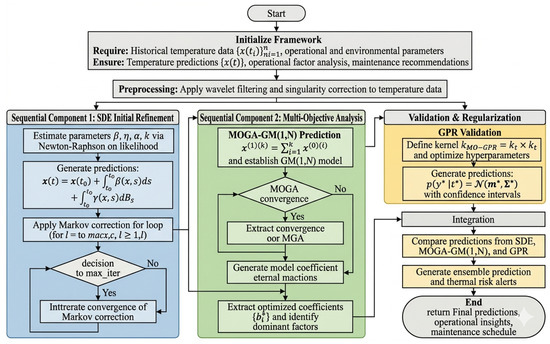
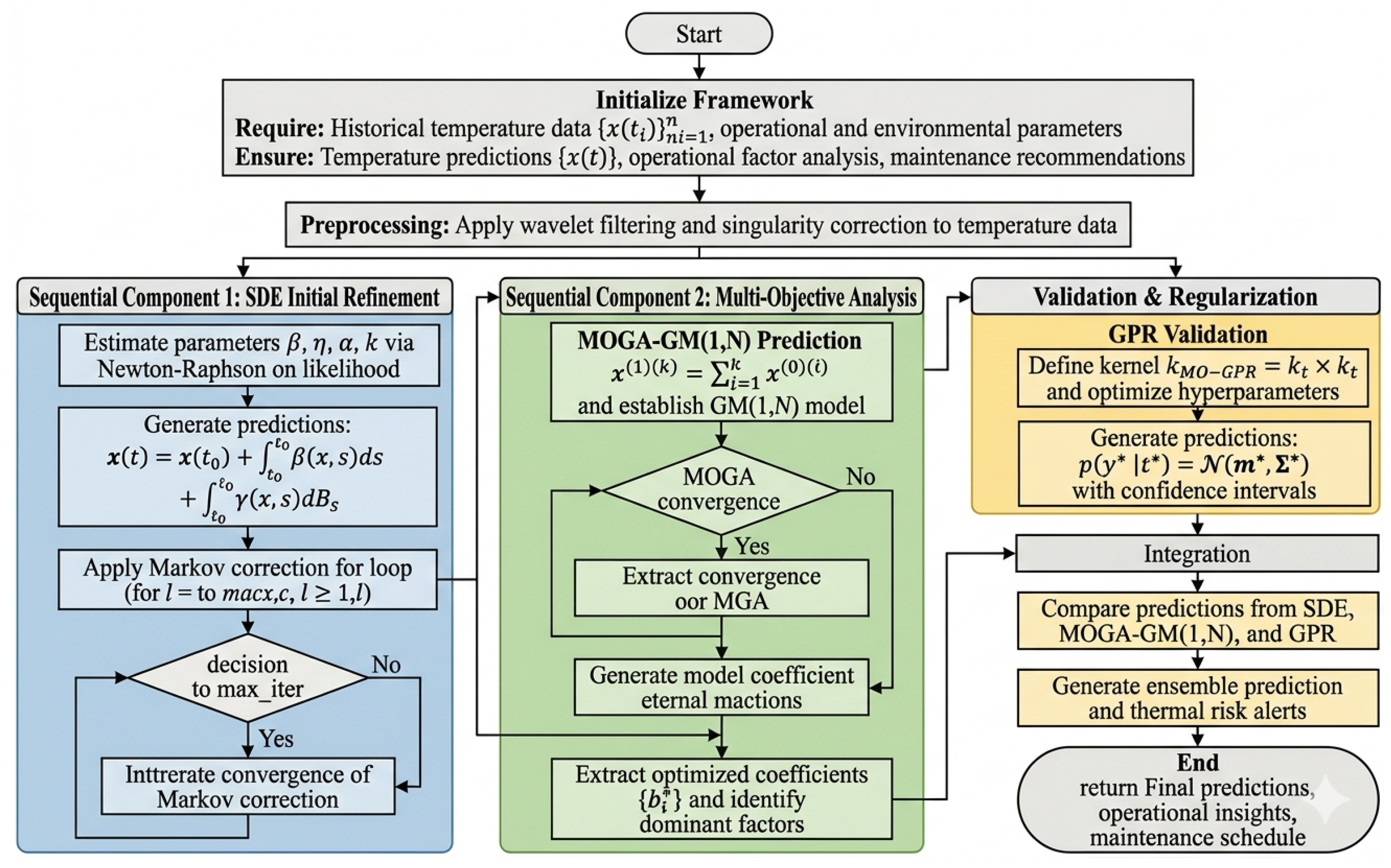
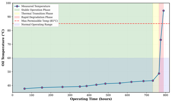
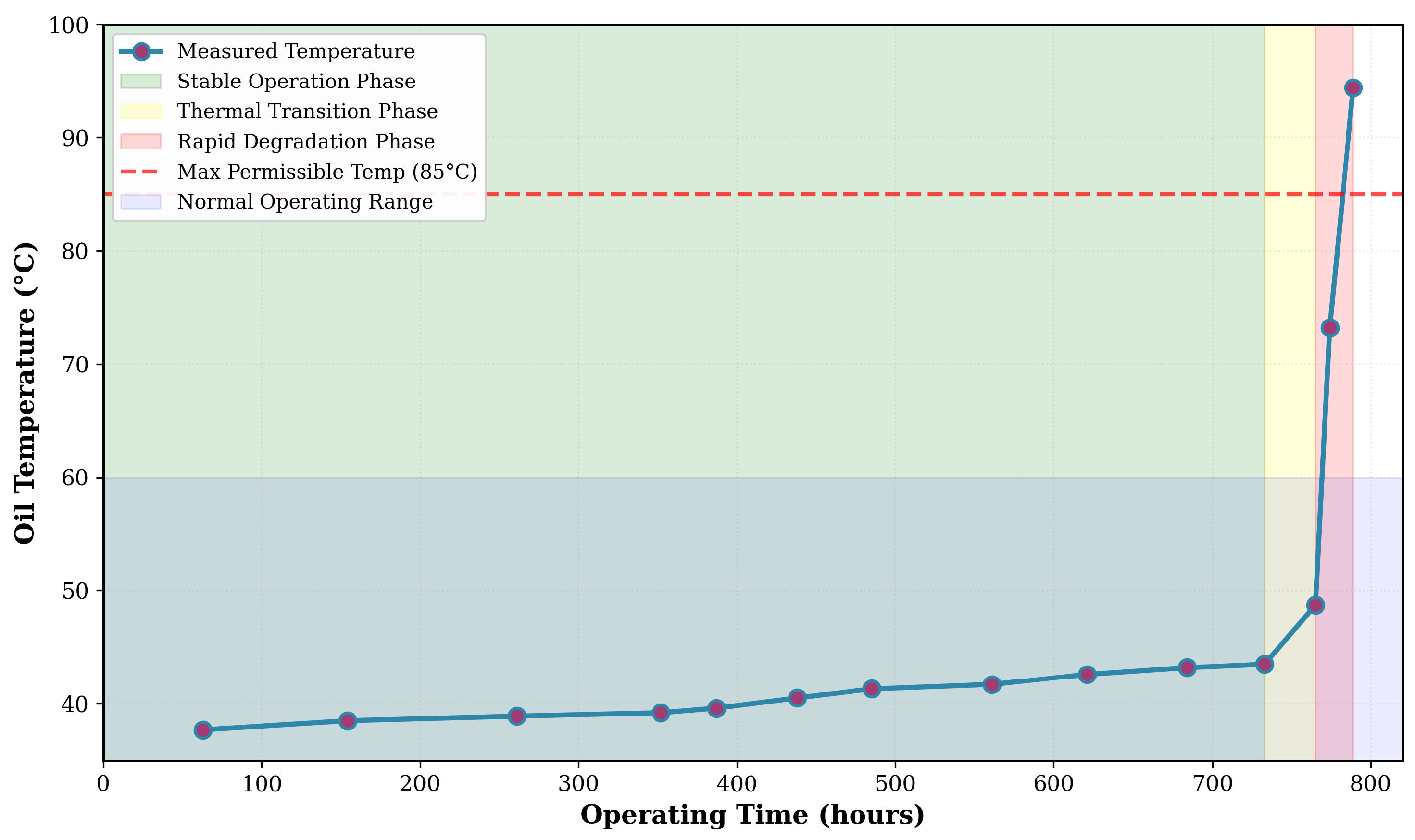
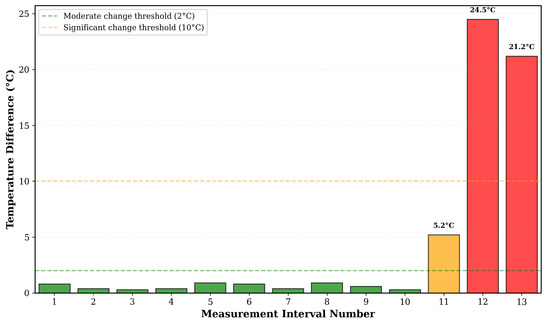
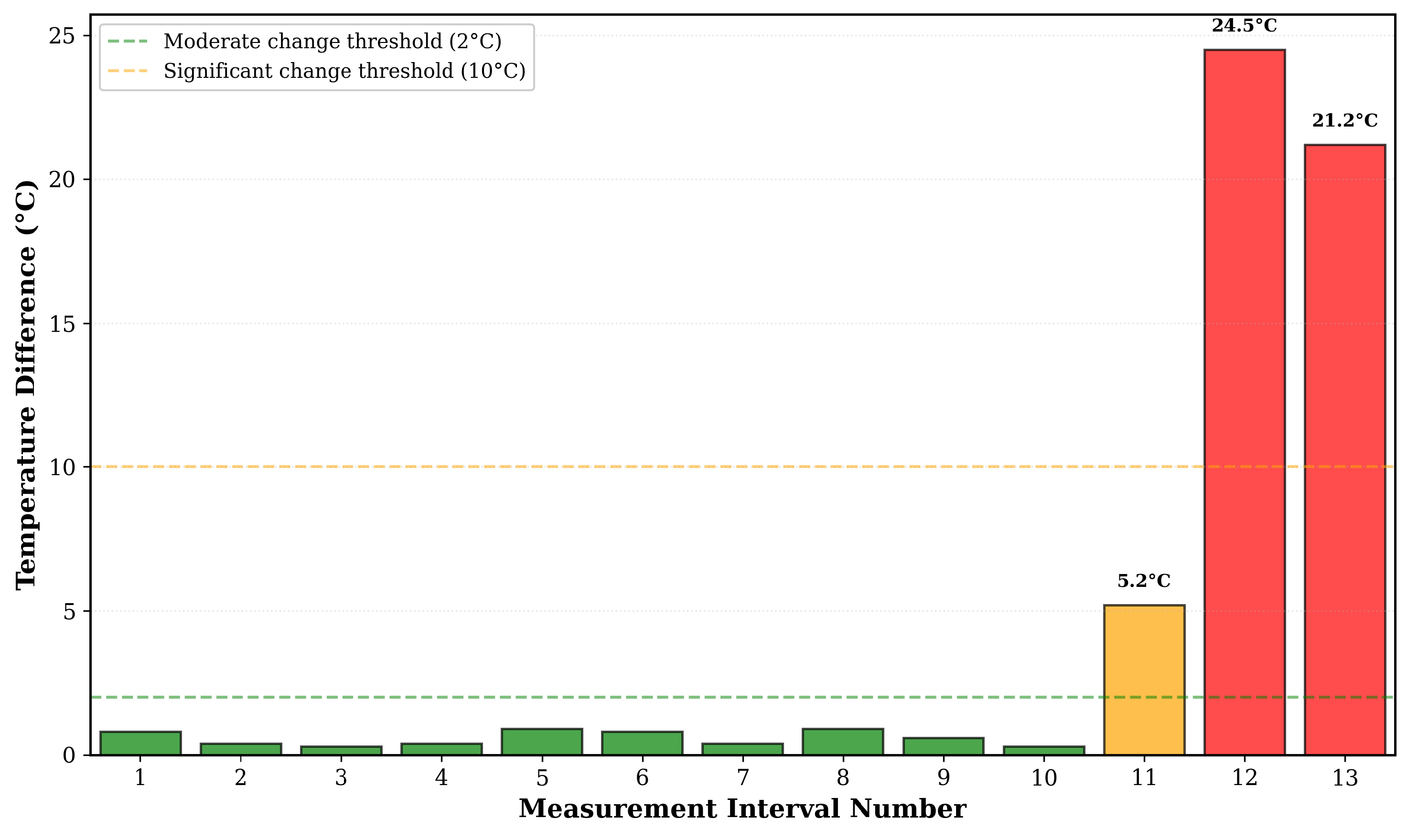
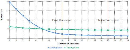
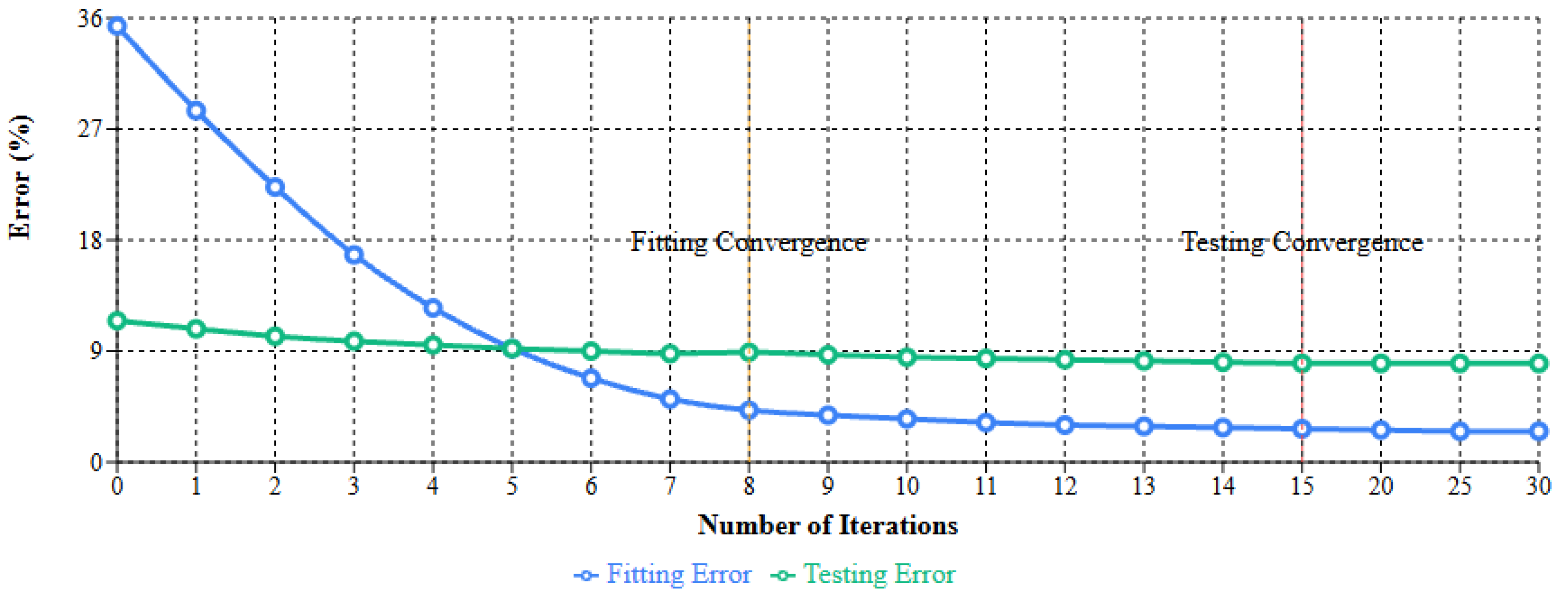
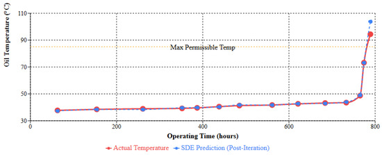
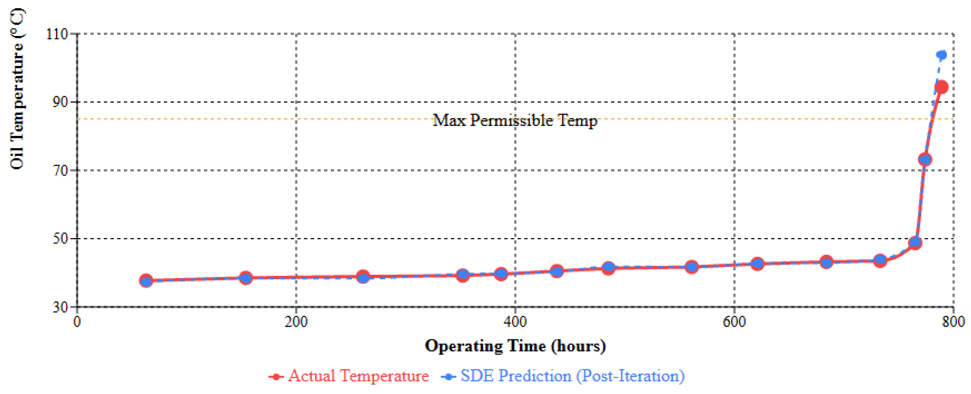

Disclaimer/Publisher’s Note: The statements, opinions and data contained in all publications are solely those of the individual author(s) and contributor(s) and not of MDPI and/or the editor(s). MDPI and/or the editor(s) disclaim responsibility for any injury to people or property resulting from any ideas, methods, instructions or products referred to in the content. |
© 2026 by the authors. Licensee MDPI, Basel, Switzerland. This article is an open access article distributed under the terms and conditions of the Creative Commons Attribution (CC BY) license.