Integrated Dynamic Modeling and Improved Deviation Coupling Control for Synchronous Motion of Multi-Joint Hydraulic Robotic Arms

Abstract

Multi-joint hydraulic robotic arms are core equipment in intelligent mining, yet their performance is often limited by strong dynamic coupling and nonlinear hydraulic effects. Traditional control methods struggle to achieve high-precision trajectory tracking and coordinated motion under high loads and flow-coupling constraints. To address these challenges, this paper establishes a coupled hydraulic–mechanical dynamic model for a multi-joint robotic arm. The mechanical dynamics are derived using the Lagrangian formulation, while the hydraulic dynamics account for flow coupling among cylinders. An improved deviation coupling control (IDCC) strategy is proposed, integrating feedforward–feedback compensation, coupling error regulation, and a flow-limiting correction term. Co-simulation in Simulink (2024b) and Amesim (2020) shows that under flow-saturation conditions, the improved strategy reduces the peak trajectory errors by approximately 47.88%, 28.08%, and 49.89% for Joints 1–3, respectively, and shortens the settling time by 27.93%. Experimental results from a three-joint hydraulic test platform confirm error reductions of 10.20–15.58% and a 31.50% decrease in overall adjustment time. The study demonstrates that the proposed control strategy effectively suppresses multi-joint coupling interferences, enhances trajectory tracking accuracy, and improves the adaptability of hydraulic robotic arms under flow-limited conditions, providing a viable solution for high-precision control in intelligent mining applications.

1. Introduction

Current mechanized mining operations are characterized by high labor intensity, low production efficiency, and significant safety risks, which severely constrain the sustainable development of the industry [1,2,3]. Intelligent transformation has become an inevitable choice for addressing the dual challenges of safety and efficiency [4,5,6]. Robotic arms, as critical equipment in intelligent mining, primarily undertake high-intensity tasks such as loading/unloading, drilling, crushing, and material handling [7,8,9]. Their operational efficiency, safety, and precision directly impact overall operational safety and production efficiency. Hydraulic drive systems have become the predominant actuation solution in mining and other engineering fields due to their prominent advantages, including high power density, strong load capacity, robustness, and low cost. However, the inherent strong nonlinearities, parameter uncertainties, and susceptibility to external environmental disturbances of hydraulic systems make traditional control methods inadequate for meeting the demands of high dynamic response and adaptive capability in the unstructured underground coal mine environment [10,11,12]. These challenges are particularly pronounced in multi-joint serial robotic arms during complex working conditions and multi-task cooperative operations, where the dynamic coupling of the hydraulic system between joints becomes a critical bottleneck for achieving high-precision, coordinated motion [13,14,15,16]. Therefore, research on the multi-joint coupling mechanisms and motion control methods for hydraulic robotic arms is not only key to enhancing equipment performance but also serves as vital technical support for advancing smart mining construction and industry-wide intelligent transformation.

For hydraulic robotic arm systems exhibiting nonlinearity, parameter uncertainties, and multi-joint coupling, traditional single-joint control methods struggle to satisfy the requirements for high-precision, coordinated motion control under high-load, dynamic environments. Consequently, researchers have continuously explored improvements and novel strategies based on traditional control algorithms. For instance, Ren et al. [17] proposed an adaptive sliding mode control method based on reinforcement learning (ASMRL), which employs a proportional-integral sliding mode (PISM) controller to address system nonlinearities while leveraging the adaptive characteristics and autonomous learning capabilities of the Deep Deterministic Policy Gradient (DDPG) algorithm to conduct parameter learning for the PISM controller. Simulation results demonstrate that this method effectively enhances trajectory tracking performance, validating the effectiveness of reinforcement learning in adaptive control of robotic manipulators. Karahan et al. [18] proposed a robust fractional-order fuzzy PID sliding mode control method for 6-DOF robotic manipulators. A hybrid tuning method integrating gray wolf optimization and particle swarm optimization (GWO-PSO) was applied to optimize controller parameters. Simulation results demonstrated that the fractional-order fuzzy PIDSMC controller achieved 91.93% improvement in mean absolute error compared to conventional PIDSMC. Wei et al. [19] proposed a hybrid neural network adaptive fuzzy sliding mode online compensatory control method with global stability for nonlinear robot systems subject to uncertainties and external disturbances. The method ensures globally uniform ultimate boundedness of all closed-loop signals and achieves convergence of neural network weights to ideal values. Simulation results showed an integral squared error of 3.24 × 10⁻⁵ rad under internal uncertainty and maximum friction disturbance, substantially improving dynamic tracking performance. Sutyasadi [20] et al. proposed a hybrid strategy integrating H∞ robust control with iterative learning control. This scheme ensures robust stability against uncertainties like load variations via the H∞ controller while utilizing iterative learning control to enhance trajectory tracking precision. Experiments showed that compared to traditional PID control, this method reduced the maximum error in sinusoidal trajectory tracking from 15° to 4°, proving particularly suitable for cost-sensitive industrial education scenarios.

However, traditional control algorithms often neglect the dynamic coupling effects of the hydraulic system between joints, leading to reduced tracking accuracy, poor synchronization, and even instability. Recently, some scholars have introduced strategies like synchronization control and cross-coupling control to address coordination issues among multiple joints of hydraulic manipulators [21,22,23]. Mu et al. [24] proposed an improved deviation coupling control method for multi-motor speed synchronization in welding robot arms. To address the complexity of the compensation mechanism in traditional deviation coupling structures, they integrated average speed and sub-average speed to optimize the speed compensator, reducing synchronization adjustment time. Research indicates that the deviation coupling control method shows promise by actively compensating for synchronization errors between joints. However, its conventional forms (typically based on PD architectures) lack the capability to handle the pronounced nonlinearities of hydraulic actuators and do not account for critical system-level constraints, most notably hydraulic flow coupling [25,26]. During the coordinated motion of multiple joints, this can lead to severe performance degradation or even complete stagnation of one or more joints, a problem not systematically addressed by existing DCC frameworks.

Although substantial research exists on the mechanical dynamics of multi-body systems [27,28,29] and the dynamics of hydraulic components [30,31], there is a notable scarcity of studies on coupled hydraulic–mechanical system models that consider the coupling within multi-joint mechanical–hydraulic systems. Beyond the control challenges, mechanical vibrations in serial robotic structures can couple with fluid-borne noise in hydraulic systems, significantly impacting tracking accuracy [32]. Moreover, proportional valves exhibit inherent nonlinearities such as dead zone and nonlinear flow–pressure characteristics [33], which are not captured by simple linear models. These factors must be considered when designing high-performance controllers for hydraulic manipulators. Establishing such a model is crucial for investigating the dynamic interaction mechanisms between hydraulic cylinder thrust maps and joint torques, and joint motion conversely affects hydraulic pressures and flows. A coupled hydraulic–mechanical system model for multi-joint hydraulic robotic arms forms the theoretical foundation for high-precision coordinated motion control. To bridge these gaps, this paper first considers the flow-coupling effects among the cylinders of different joints to establish a coupled hydraulic–mechanical dynamic model for multi-joint hydraulic robotic arms. Subsequently, an improved deviation coupling control (IDCC) strategy is proposed. This strategy integrates a feedforward–feedback composite controller to compensate for key nonlinearities and innovatively incorporates a flow correction term to dynamically adjust control gains. Finally, co-simulation and experimental tests on a three-joint hydraulic robotic arm are conducted to validate the effectiveness of the proposed modeling and control approaches in terms of trajectory tracking accuracy and coordinated motion performance. The research presented in this paper contributes to improving the trajectory tracking and coordinated motion capabilities of multi-joint hydraulic robotic arms, thereby enhancing their adaptability in complex working conditions.

2. Dynamic Modeling of Multi-Joint Robotic Manipulators

2.1. Mechanical Dynamic Modeling for Multi-Joint Robotic Manipulators

For multi-degree-of-freedom robotic manipulators, strong interactions between joints often result in complex inertial coupling, Coriolis forces, and gravitational effects, rendering the direct application of Newton’s equations cumbersome. Therefore, this paper adopts the Lagrangian method to establish the mechanical dynamic model of the multi-joint manipulator system. First, the Lagrangian function L of the system is constructed, which is defined as the difference between the total kinetic energy and the total potential energy of the system [34]:

$$L=T-V$$

(1)

where $T$ and $V$ represent the total kinetic energy and potential energy of the system, respectively. According to the Alembert principle, the system’s dynamic equations can be derived from the Lagrange equation:

$${\displaystyle \frac{d}{dt}}\left({\displaystyle \frac{\partial L}{\partial {\dot{q}}_i}}\right)-{\displaystyle \frac{\partial L}{\partial q_i}}={\tau }_i$$

(2)

where $q_i$ represents the generalized coordinates of the system, which for the robotic arm correspond to its joint angles ${\theta }_i$; ${\dot{q}}_i$ is their first derivative with respect to time, i.e., the generalized velocities ${\dot{\theta }}_i$ representing the joint angular velocities of the robotic arm. ${\tau }_i$ denotes the generalized forces, which for the robotic arm are the joint driving torques supplied by hydraulic cylinders, serving as the joint input torques.

Assuming the robotic arm consists of n joints, with each link i having mass mᵢ and moment of inertia Iᵢ, the system kinetic energy includes both translational and rotational components. The translational kinetic energy of a rigid body is

$$T_{trans,i}={\displaystyle \frac{1}{2}}{m}_i{v}_i^2$$

(3)

where $v_i$ is the velocity of the center of mass of the i-th link, computable via forward kinematics. The rotational kinetic energy of a rigid body is as follows:

$$T_{rot,i}={\displaystyle \frac{1}{2}}{I}_i{\dot{\theta }}_i^2$$

(4)

where $I_i$ is the inertia tensor of the link about its center of mass.

Thus, the total kinetic energy of the robotic arm is

$$T={\displaystyle \sum _{i=1}^n\left(\frac{1}{2}{m}_i{v}_i^2+\frac{1}{2}{I}_i{\dot{\theta }}_i^2\right)}$$

(5)

For the hydraulic robotic arm studied in this paper, which can be regarded as a three-link manipulator, the velocity of the center of mass can be expressed as follows:

$$v_i^2={\dot{\theta }}_1^2{f}_1\left(\theta \right)+{\dot{\theta }}_2^2{f}_2\left(\theta \right)+{\dot{\theta }}_3^2{f}_3\left(\theta \right)+2{\dot{\theta }}_1{\dot{\theta }}_2{f}_{12}\left(\theta \right)+2{\dot{\theta }}_1{\dot{\theta }}_2{f}_{13}\left(\theta \right)+2{\dot{\theta }}_2{\dot{\theta }}_3{f}_{23}\left(\theta \right)$$

(6)

where $f_i\left(\theta \right)$ is a function determined by the geometric relationship of the robotic arm.

The potential energy is primarily composed of gravitational potential energy:

$$V={\displaystyle \sum _{i=1}^n{m}_{i}g{h}_i}$$

(7)

where $h_i$ is the height of the center of mass of the i-th link, typically calculated from the geometric parameters of the robotic arm.

Substituting Equations (5) and (7) into Equation (2) yields the mechanical dynamic equation of the robotic arm:

$$M\left(\theta \right)\ddot{\theta }+C\left(\theta ,\dot{\theta }\right)\dot{\theta }+G\left(\theta \right)=\tau$$

(8)

where $M\left(\theta \right)$ is the inertia matrix, describing the mass distribution and inertial coupling among the joints; $C\left(\theta ,\dot{\theta }\right)$ is the Coriolis and centrifugal force matrix; $G\left(\theta \right)$ is the gravity vector, representing the gravitational effects on the system; and $\tau$ is the vector of external input torques, provided by the hydraulic drive in the hydraulic robotic arm.

For the three-joint robotic arm studied in this paper, the expanded component form of its dynamic equations is as follows:

$$\left\{\begin{array}{l}{M}_{11}{\ddot{\theta }}_1+M_{12}{\ddot{\theta }}_2+M_{13}{\ddot{\theta }}_3+C_{11}{\dot{\theta }}_1+C_{12}{\dot{\theta }}_2+C_{13}{\dot{\theta }}_3+G_1={\tau }_1\\ M_{21}{\ddot{\theta }}_1+M_{22}{\ddot{\theta }}_2+M_{23}{\ddot{\theta }}_3+C_{21}{\dot{\theta }}_1+C_{22}{\dot{\theta }}_2+C_{23}{\dot{\theta }}_3+G_2={\tau }_2\\ M_{31}{\ddot{\theta }}_1+M_{32}{\ddot{\theta }}_2+M_{33}{\ddot{\theta }}_3+C_{31}{\dot{\theta }}_1+C_{32}{\dot{\theta }}_2+C_{33}{\dot{\theta }}_3+G_3={\tau }_3\end{array}\right.$$

(9)

In the inertia matrix:

$$\left\{\begin{array}{l}{M}_{11}=I_1+m_1{l}_{c1}^2+m_2{l}_1^2+m_3{l}_1^2\\ M_{12}=M_{21}=m_2{l}_1{l}_{c2}\cos \left({\theta }_2\right)+m_3{l}_1{l}_2\cos \left({\theta }_2\right)\\ M_{13}=M_{31}=m_3{l}_1{l}_{c3}\cos \left({\theta }_2+{\theta }_3\right)\\ M_{22}=I_2+m_2{l}_{c2}^2+m_3{l}_2^2\\ M_{23}=M_{32}=m_3{l}_2{l}_{c3}\cos \left({\theta }_3\right)\\ M_{33}=I_3+m_3{l}_{c3}^2\end{array}\right.$$

(10)

where $M_{ii}$ is the equivalent moment of inertia of joint i; $M_{ij}$ represents the inertial coupling between joint i and joint j; $l_{ci}$ is the distance from the center of mass of the i-th link to joint I; $m_i$ is the mass of the i-th link; $l_i$ is the length of the i-th link; and ${\theta }_i$ is the rotation angle of the i-th joint.

The Coriolis matrix is calculated via partial derivatives of the inertia matrix, and its components are as follows:

$$C_{ij}={\displaystyle \sum _{k=1}^3\frac{1}{2}\left(\frac{\partial M_{ik}}{\partial {\theta }_j}+\frac{\partial M_{jk}}{\partial {\theta }_i}-\frac{\partial M_{ij}}{\partial {\theta }_k}\right)}{\dot{\theta }}_k$$

(11)

It can be obtained that

$$\left\{\begin{array}{l}{C}_{11}=-m_2{l}_1{l}_{c2}\sin \left({\theta }_2\right){\dot{\theta }}_2-m_3{l}_1{l}_{c3}\sin \left({\theta }_2+{\theta }_3\right)\left({\dot{\theta }}_2+{\dot{\theta }}_3\right)\\ C_{12}=-m_2{l}_1{l}_{c2}\sin \left({\theta }_2\right){\dot{\theta }}_1\\ C_{13}=-m_3{l}_1{l}_{c3}\sin \left({\theta }_2+{\theta }_3\right){\dot{\theta }}_1\\ C_{21}=m_2{l}_1{l}_{c2}\sin \left({\theta }_2\right){\dot{\theta }}_2\\ C_{22}=-m_3{l}_2{l}_{c3}\sin \left({\theta }_3\right){\dot{\theta }}_3\\ C_{23}=-m_3{l}_2{l}_{c3}\sin \left({\theta }_3\right)\left({\dot{\theta }}_2+{\dot{\theta }}_3\right)\\ C_{31}=m_3{l}_1{l}_{c3}\sin \left({\theta }_2+{\theta }_3\right){\dot{\theta }}_1\\ C_{32}=m_3{l}_2{l}_{c3}\sin \left({\theta }_3\right){\dot{\theta }}_2\\ C_{33}=0\end{array}\right.$$

(12)

where $C_{ii}$ represents the Coriolis contribution of joint i to itself, and $C_{ij}$ represents the Coriolis contribution of joint j to joint i.

The gravity terms G_i are, respectively,

$$\left\{\begin{array}{l}{G}_1=\left(m_1{l}_{c1}+m_2{l}_1+m_3{l}_1\right)g\cos {\theta }_1\\ G_2=\left(m_2{l}_{c2}+m_3{l}_2\right)g\cos {\theta }_2\\ G_3=m_3{l}_{c3}g\cos {\theta }_3\end{array}\right.$$

(13)

2.2. Hydraulic Dynamics Modeling of Multi-Joint Robotic Manipulator Systems

In multi-joint systems, multiple hydraulic cylinders share a common hydraulic pump, leading to flow-coupling effects among the cylinders. Due to varying loads and flow demands across the cylinders, the actual flow may deviate from the desired flow, thereby affecting the system’s control accuracy and dynamic response characteristics. Therefore, it is essential to account for the mutual interactions among multiple hydraulic cylinders and establish a hydraulic system model suitable for multi-joint applications.

The hydraulic system is driven by a motor–gear pump unit. Considering the dynamic characteristics of the motor and the mechanical properties of the gear pump, the relationship between the electromagnetic torque and the rotational speed of the motor is given by the following [35]:

$$J_m{\displaystyle \frac{d{\omega }_p}{dt}}=T_m-D_p\left(P_p-P_t\right)-B_v{\omega }_p$$

(14)

where $J_m$ is the total moment of inertia of the motor rotor and the pump; $T_m=K_{t}i$ is the motor driving torque, with K_i as the torque constant and i as the armature current; $D_p$ is the displacement of the gear pump; $P_p$ is the pump outlet pressure; $P_t$ is the tank pressure (usually set to 0); $B_v$ is the viscous friction coefficient; and ${\omega }_p$ is the rotational speed of the pump.

Considering the global pressure model with multi-actuator coupling:

$${\displaystyle \frac{d{P}_p}{dt}}={\displaystyle \frac{{\beta }_e}{V_t}}\left(Q_p-{\displaystyle \sum _{i=1}^3{Q}_i}-Q_{leak}\right)$$

(15)

where ${\beta }_e$ is the effective bulk modulus of the hydraulic fluid, which is assumed to be constant in this model due to the limited variation within the typical operating pressure range (5–10 MPa) [36]; $V_t$ is the total oil-containing volume of the system; $Q_i$ is the flow demand of the i-th actuator; and $Q_{leak}=K_s{P}_p$ represents the total system leakage flow, with $K_s$ as the leakage coefficient.

The system state variables are defined as follows:

$$X={\left[{\omega }_p,P_p,P_{L1},P_{L2},P_{L3},L_1,L_2,L_3,v_1,v_2,v_3\right]}^T$$

(16)

The nonlinear state equations of the system are established as follows:

$$\dot{X}=\left\{\begin{array}{l}{\displaystyle \frac{d{\omega }_p}{dt}}=\left[K_{t}i-D_p{P}_p-B_v{\omega }_p\right]/J_m\\ {\displaystyle \frac{d{P}_p}{dt}}={\displaystyle \frac{{\beta }_e}{V_t}}\left[D_p{\omega }_p-{\displaystyle \sum _{i=1}^3{C}_d{\omega }_i{x}_i\sqrt{\frac{2}{\rho }\left(P_p-P_{Li}\right)}}\right]\\ {\displaystyle \frac{d{P}_{Li}}{dt}}={\displaystyle \frac{{\beta }_e}{A_i{L}_i}}\left[Q_i-A_i{v}_i-C_{ip}\left(P_{Li}-P_{Lj}\right)\right]\\ {\displaystyle \frac{d^2{L}_i}{d{t}^2}}=\left[A_i{P}_{Li}-B_i{v}_i-K_i{L}_i-F_c\right]/M_i\end{array}\right.$$

(17)

where $F_c$ is the coupling force term:

$$M_i{\ddot{L}}_i+B_i{\dot{L}}_i+K_i{L}_i+F_c=A_i{P}_{Li}$$

(18)

$$F_c={\displaystyle \sum _{j\ne i}{K}_{ij}\left(L_i-L_j\right)}+C_{ij}\left({\dot{L}}_i-{\dot{L}}_j\right)$$

(19)

The flow–pressure coupling matrix is as follows:

$$\left[{\displaystyle \frac{\partial Q_i}{\partial P_p}}\right]=\left|\begin{array}{ccc}{\displaystyle \frac{C_d{\omega }_1{x}_1}{\sqrt{2\rho \left(P_p-P_{L1}\right)}}}& 0& 0\\ 0& {\displaystyle \frac{C_d{\omega }_2{x}_2}{\sqrt{2\rho \left(P_p-P_{L2}\right)}}}& 0\\ 0& 0& {\displaystyle \frac{C_d{\omega }_3{x}_3}{\sqrt{2\rho \left(P_p-P_{L3}\right)}}}\end{array}\right|$$

(20)

2.3. Dynamics of the Coupled Model for the Hydraulic–Mechanical System with a Multi-Joint Robotic Manipulator

The dynamics model of the mechanical system describes the motion characteristics of each joint, including the effects of inertia, damping, gravity, and other factors on joint motion, while the dynamics model of the hydraulic system involves factors such as hydraulic pumps, hydraulic cylinders, and valve-controlled flow rates, which determine the thrust provided by the hydraulic cylinders and their dynamic response. Since the motion of the hydraulic cylinders directly drives the joints of the robotic arm, and their thrust is transmitted through linkage mechanisms to produce joint torques, it is necessary to establish the mapping relationship between the thrust of the hydraulic cylinders and the motion state of the joints. The thrust provided by the hydraulic system can be converted into an equivalent torque acting on the joints via the Jacobian matrix, which is then substituted into the dynamics equations of the mechanical system to model the coupling relationship between the hydraulic and mechanical systems.

Let the variables of the three joints be $q=\left[{\theta }_1,{\theta }_2,{\theta }_3\right]$ and the lengths of the three links be $L_1$, $L_2$, $L_3$. Within the working plane of the three joints, the end-effector position $\left(x,y\right)$ can be computed through forward kinematics:

$$\left\{\begin{array}{l}x=L_1\cos {\theta }_1+L_2\cos \left({\theta }_1+{\theta }_2\right)+L_3\cos \left({\theta }_1+{\theta }_2+{\theta }_3\right)\\ y=L_1\sin {\theta }_1+L_2\sin \left({\theta }_1+{\theta }_2\right)+L_3\sin \left({\theta }_1+{\theta }_2+{\theta }_3\right)\end{array}\right.$$

(21)

The Jacobian matrix $J$ is composed of the partial derivatives of the position with respect to the joint angles:

$$J={\displaystyle \frac{\partial (x,y)}{\partial ({\theta }_1,{\theta }_2,{\theta }_3)}}=\left[\begin{array}{ccc}{\displaystyle \frac{\partial x}{\partial {\theta }_1}}& {\displaystyle \frac{\partial x}{\partial {\theta }_2}}& {\displaystyle \frac{\partial x}{\partial {\theta }_3}}\\ {\displaystyle \frac{\partial y}{\partial {\theta }_1}}& {\displaystyle \frac{\partial y}{\partial {\theta }_2}}& {\displaystyle \frac{\partial y}{\partial {\theta }_3}}\end{array}\right]$$

(22)

Taking partial derivatives of x and y:

$$\begin{gathered} {\displaystyle \frac{\partial x}{\partial {\theta }_1}}=-L_1\sin {\theta }_1-L_2\sin \left({\theta }_1+{\theta }_2\right)-L_3\sin \left({\theta }_1+{\theta }_2+{\theta }_3\right) \\ {\displaystyle \frac{\partial x}{\partial {\theta }_2}}=-L_2\sin \left({\theta }_1+{\theta }_2\right)-L_3\sin \left({\theta }_1+{\theta }_2+{\theta }_3\right) \\ {\displaystyle \frac{\partial x}{\partial {\theta }_3}}=-L_3\sin \left({\theta }_1+{\theta }_2+{\theta }_3\right) \\ {\displaystyle \frac{\partial y}{\partial {\theta }_1}}=L_1\cos {\theta }_1+L_2\cos \left({\theta }_1+{\theta }_2\right)+L_3\cos \left({\theta }_1+{\theta }_2+{\theta }_3\right) \\ {\displaystyle \frac{\partial y}{\partial {\theta }_2}}=L_2\cos \left({\theta }_1+{\theta }_2\right)+L_3\cos \left({\theta }_1+{\theta }_2+{\theta }_3\right) \\ {\displaystyle \frac{\partial y}{\partial {\theta }_3}}=L_3\cos \left({\theta }_1+{\theta }_2+{\theta }_3\right) \end{gathered}$$

(23)

Substituting into Equation (22) yields the final Jacobian matrix. The defining equation for the Jacobian matrix is as follows:

$$\dot{x}=J\dot{q}$$

(24)

where $\dot{x}$ is the end-effector velocity, and $\dot{q}$ is the angular velocity.

By transposing the Jacobian matrix, the coupling relationship between the hydraulic system and the mechanical system is established through Equation (24):

$$\tau =J^{T}F$$

(25)

where $\tau$ is the torque exerted by the hydraulic cylinders on the joints, and $F$ is the thrust provided by the hydraulic cylinders:

$$F_i=P_{Li}{A}_i-P_{Bi}{A}_{Bi}-F_{fi}$$

(26)

where $F_i$ is the thrust exerted by the i-th hydraulic cylinder on the mechanical system, $P_{Li}$ and $P_{Bi}$ are the pressures in the two chambers of the cylinder, $A_i$ and $A_{Bi}$ are the effective piston areas on the respective sides, and $F_{fi}$ represents frictional forces.

Therefore, the dynamics equation of the multi-joint robotic arm system can be expressed as follows:

$$M\left(\theta \right)\ddot{\theta }+C\left(\theta ,\dot{\theta }\right)\dot{\theta }+G\left(\theta \right)=J^{T}F$$

(27)

Through the above equation, the mechanical system and the hydraulic system are integrated, achieving system modeling for the multi-joint hydraulic robotic arm.

3. Design of Improved Deviation Coupling Control Strategy

3.1. Design of the Controller

In the synchronous control of multi-joint robotic arms, deviation coupling control is a method that reduces synchronization error by introducing error coupling terms between joints. It not only controls the motion error of each joint individually but also prioritizes the joint with the largest error, guiding the errors of other joints to converge toward it, thereby minimizing the overall synchronization deviation of the system. This control strategy calculates the control errors of all joints, compares them mutually, and feeds the resulting information back as compensation to each joint’s controller. The motion state of each joint is dynamically adjusted according to these compensation signals, ensuring the overall coordination and stability of the robotic arm’s movement.

In the three-joint robotic arm studied in this paper, each joint is driven by a corresponding hydraulic cylinder. The control objective is to ensure that each joint’s angular displacement ${\theta }_i\left(i=1,2,3\right)$ follows the desired trajectory ${\theta }_{di}\left(i=1,2,3\right)$ while reducing the relative errors between joints. The tracking errors for the three joints are as follows:

$$\left\{\begin{array}{l}{e}_1={\theta }_{d1}-{\theta }_1\\ e_2={\theta }_{d2}-{\theta }_2\\ e_3={\theta }_{d3}-{\theta }_3\end{array}\right.$$

(28)

When controlling the system, it is necessary to consider not only the tracking error of each joint but also the mutual influence among the three joints. When one joint deviates from its desired trajectory due to various disturbances, the other two joints in the system are also affected and need to adjust their motion to minimize the impact of the disturbance as much as possible. Let the synchronization error between two joints $i$ and $j$ be ${\epsilon }_i$:

$$\epsilon =Te=\left[\begin{array}{ccc}1& -1& 0\\ 0& 1& -1\\ -1& 0& 1\end{array}\right]\left[\begin{array}{c}{e}_1\\ e_2\\ e_3\end{array}\right]$$

(29)

Define the coupled error as follows:

$$E=e+\beta \epsilon$$

(30)

Substituting Equation (29) into Equation (30) yields

$$E=\left(I+\beta T\right)e$$

(31)

where I is the identity matrix and $\beta$ is the coupling compensation coefficient matrix.

When $0<\beta \le 1$, a larger $\beta$ indicates a stronger synchronization control effect. If $E$ can converge to 0, then $e$ and $\epsilon$ can also converge to 0, indicating that the goal of system synchronization control can be achieved.

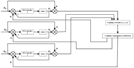
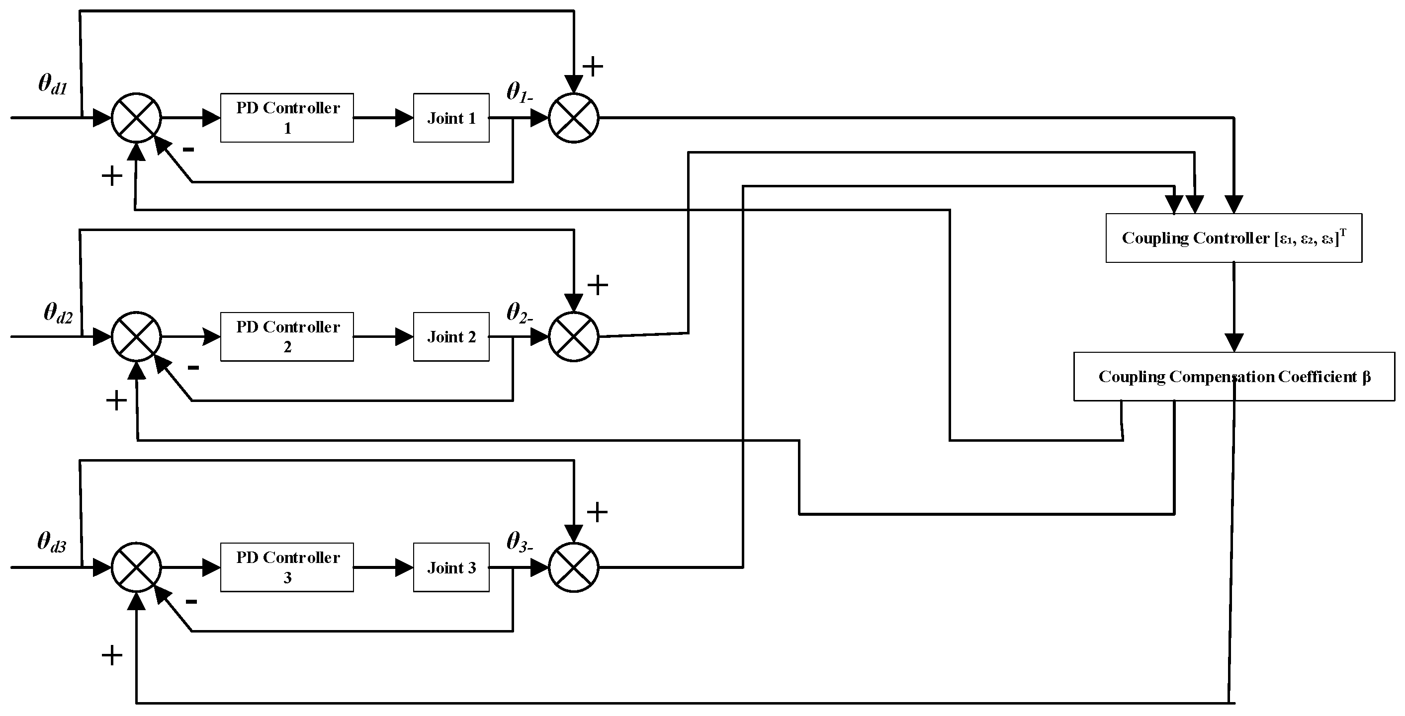
The traditional PD-based deviation coupling control structure is shown in Figure 1. Compared to the traditional deviation coupling control, this paper designs a deviation coupling control strategy based on feedforward–feedback composite control and introduces a correction term under flow limitation to optimize flow distribution and improve control precision. The control strategy consists of three parts: feedforward–feedback composite control, deviation coupling control, and the flow limitation correction term.

Figure 1. Deviation coupling control structure diagram.

Feedforward–Feedback Composite Control Design

For a single-joint hydraulic system, considering nonlinear factors such as the dead zone of the proportional directional valve and load disturbances, a feedforward–feedback composite control is adopted:

$${\tau }_i=u_c+u_i^{ff}+u_i^{fb}$$

(32)

where the feedforward control term $u_c$ is primarily used to compensate for dead zone nonlinearity and improve response speed. The feedforward control term $u_i^{ff}$ is mainly used to compensate for the impact of load disturbances on system control, enhancing the system’s anti-disturbance capability.

The feedback control term $u_i^{fb}$ employs PD control:

$$u_i^{fb}=K_{pi}{e}_i+K_{di}{\dot{e}}_i$$

(33)

where $K_{pi}$ is the proportional gain and $K_{di}$ is the derivative gain.

Introducing coupling gains $K_{ci}$ for error compensation on the coupled error $E$:

$${\tau }_i=u_c+u_i^{ff}+u_i^{fb}+K_{ci}{E}_i$$

(34)

Due to the total flow limitation of the hydraulic system, it cannot guarantee sufficient flow for all joints simultaneously. Therefore, a flow allocation correction term is added to the controller. The system’s total flow demand $Q_t$ is as follows:

$$Q_t={\displaystyle \sum _{i=1}^3{Q}_i}$$

(35)

The system’s maximum supply flow is $Q_m$. Calculate the flow adjustment coefficient:

$$\lambda =\min \left(1,{\displaystyle \frac{Q_{\mathrm{m}}}{Q_t}}\right)$$

(36)

When the system’s supply flow is sufficient, i.e., $Q_t\le Q_m$, κ = 1, indicating that the hydraulic pump’s supply capacity is sufficient. All hydraulic cylinders can obtain the required flow without adjustment. When the system’s supply flow is insufficient, i.e., $Q_t>Q_m$, κ < 1, indicating that the hydraulic pump’s supply capacity is insufficient. It is necessary to proportionally reduce the flow demand of all hydraulic cylinders to adapt to the pump’s maximum supply capacity. The control gains are corrected as follows:

$$K_{ci}^n=K_{ci}·\lambda$$

(37)

The final control input is

$${\tau }_i=u_c+u_i^{ff}+u_i^{fb}+K_{ci}^n{E}_i$$

(38)

Here, when flow is sufficient, the control law remains unchanged. When flow is limited, the control gains for all joints are automatically reduced to prevent the total flow from exceeding the capacity. This action effectively limits the commanded velocities, preventing abrupt flow starvation that could cause pressure spikes. By smoothing the gain transition (κ varies continuously), the controller avoids inducing shock waves in the hydraulic circuit.

3.2. Stability Analysis

The system error equation is

$$e_i={\theta }_{di}-\theta$$

(39)

Combining the derived dynamic equation and the control input yields the following:

$$M_i{\ddot{\theta }}_i+C_i{\dot{\theta }}_i+K_i{\theta }_i=u_c+u_i^{ff}+u_i^{fb}+K_{ci}^n{E}_i$$

(40)

where $K_i$ represents the stiffness term, used to simulate the effect of gravity.

Rewriting it as an error equation:

$$M_i{\ddot{e}}_i+C_i{\dot{e}}_i+K_i{e}_i=u_c+u_i^{ff}+K_{pi}{e}_i+K_{di}{\dot{e}}_i+K_{ci}^n{E}_i$$

(41)

Constructing a Lyapunov function:

$$V={\displaystyle \frac{1}{2}}{\displaystyle \sum _{i=1}^3\left(M_i{\dot{e}}_i^2+K_i{e}_i^2\right)}$$

(42)

Taking the derivative with respect to time and simplifying yields the following:

$$\dot{V}={\displaystyle \sum _{i=1}^3-C_i{\dot{e}}_i^2+K_{pi}{e}_i{\dot{e}}_i+K_{di}{\dot{e}}_i^2+K_{ci}^n{E}_i{\dot{e}}_i}$$

(43)

When constructing a Lyapunov function, if $C_i>0$, $K_{di}>0$, and $K_{pi}$ is chosen appropriately, then $\dot{V}\le 0$, indicating that the error ultimately converges and the system is stable. Therefore, using the Lyapunov method, it can be proven that with reasonable selection of control gains, the system error can converge, i.e., the joint synchronization error eventually tends to zero, ensuring high-precision synchronous control of the robotic arm. In practical hydraulic systems, sensor acquisition and controller computation introduce delays that may affect stability margins. However, because the proposed IDCC incorporates feedforward compensation and the gain scaling κ is updated slowly relative to the system bandwidth, the closed-loop system retains robustness against small delays.

In the case of flow saturation, the gain scaling factor κ becomes time-varying (κ(t) ≤ 1). Since κ(t) is bounded and its variation rate is limited by the physical dynamics of the hydraulic system, the Lyapunov function derivative $\dot{V}$ remains negative provided the baseline gains $K_{pi}$ and $K_{di}$ are sufficiently large. The term (1 − κ(t)) acts as a temporary reduction in the effective gains, but it does not destroy the sign-definiteness of $\dot{V}$ because κ(t) never exceeds 1. Therefore, the system remains asymptotically stable even under flow-limited conditions, though the convergence rate may temporarily decrease.

4. Simulation Analysis of Multi-Joint Synchronous Control Strategy

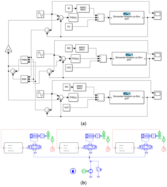
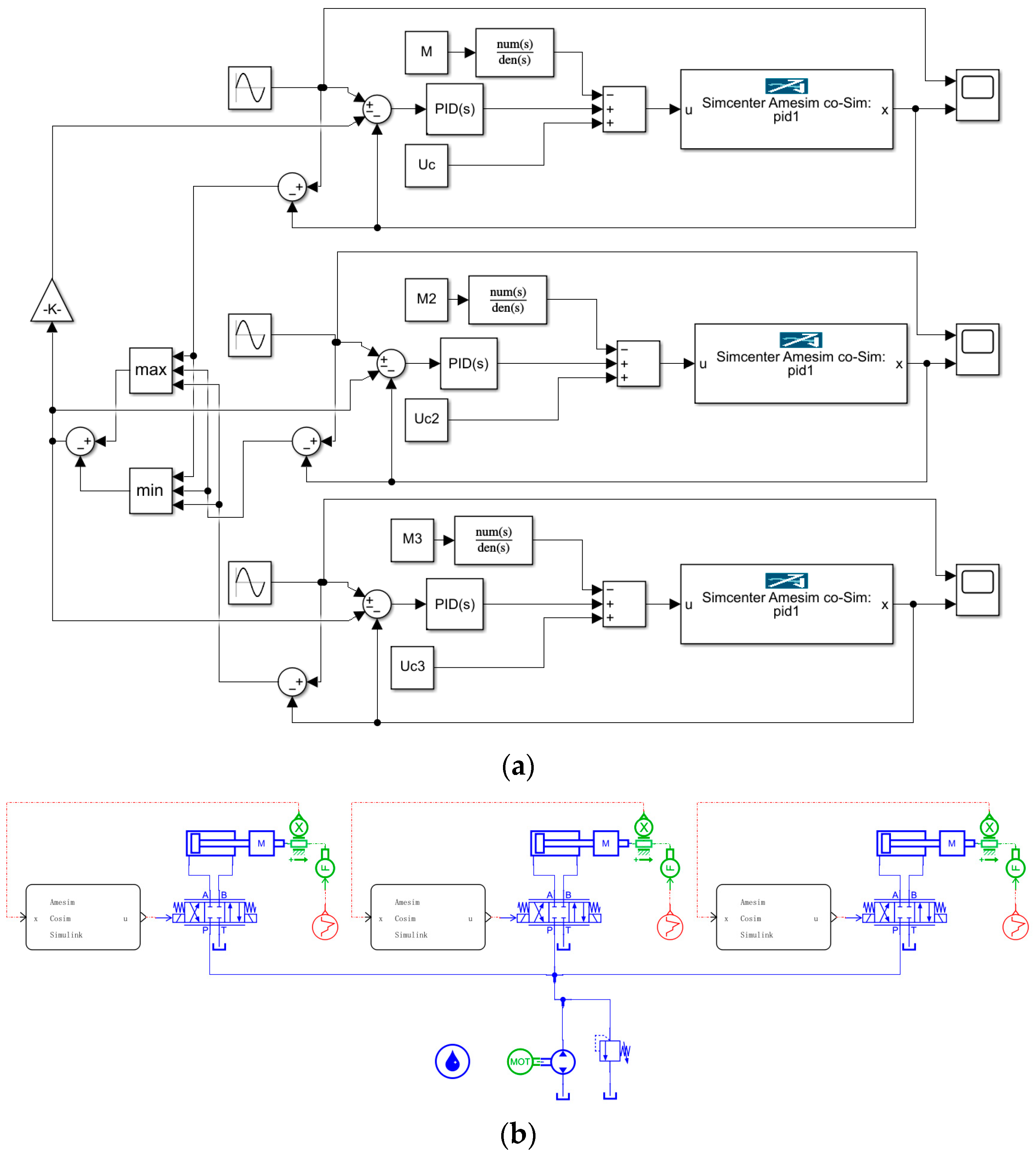
To verify the effectiveness of the improved deviation coupling control strategy designed earlier, a co-simulation model of the multi-joint system using Simulink (2024b) and Amesim (2020) was used, as shown in Figure 2. In Simulink, the dynamics model of multi-joint robotic manipulators was established based on the derived dynamic equations in this paper (Figure 2a). Figure 2b shows a multi-joint hydraulic model in Amesim, which is driven by a single pump that operates three hydraulic cylinders. The relevant parameters of components such as the hydraulic pump, motor, and proportional valve are listed in Table 1.

Figure 2. Co-simulation model of the multi-joint system using Simulink and Amesim: (a) deviation coupling control simulation model in Simulink; (b) multi-joint hydraulic model in Amesim.

Table 1. Amesim simulation parameters for multi-joint system.

Parameter	Value
Motor RPM (r/min)	1500
Pump Displacement (cc/rev)	10
Proportional Valve Pressure Drop (bar)	10
Relief Valve Cracking Pressure (Mpa)	8

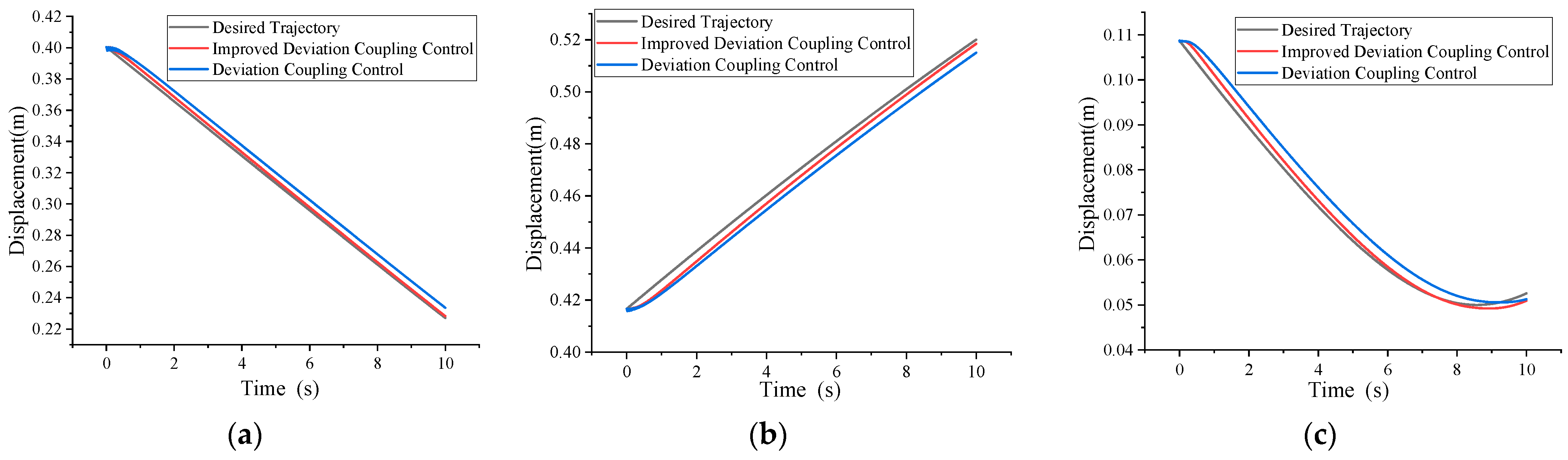
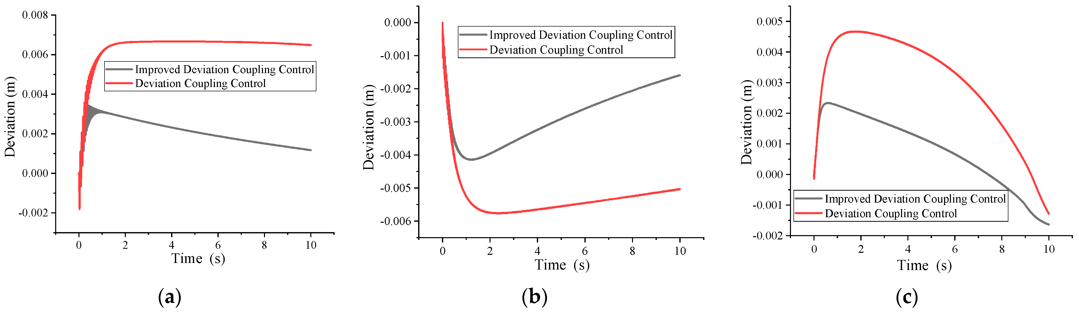
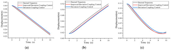
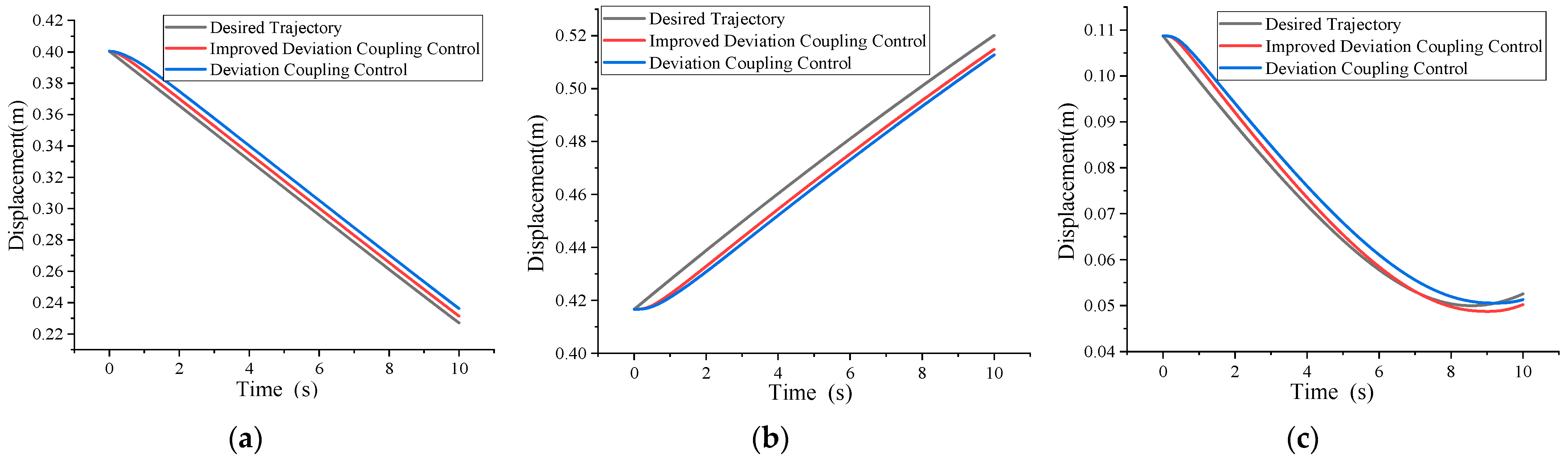
Using the planned displacement curves (Figure 3) for each joint as the motion control target for the robotic arm, a Simulink–Amesim co-simulation was performed on the established robotic arm model. The trajectory deviation is shown in Figure 4. For Joint 1 of the robotic arm, using deviation coupling control, at the start of control, the driving hydraulic cylinder’s displacement oscillates, and the error fluctuates up and down, showing an overall increasing trend. At 1.84 s, the error reaches 6.60 mm, then stabilizes around 6.60 mm. Using the improved deviation coupling control, at the start of control, the driving hydraulic cylinder’s displacement also oscillates. At 0.4 s, it reaches the maximum deviation of 3.44 mm, after which the error gradually decreases. The improved deviation coupling control reduces the peak error of Joint 1 by approximately 47.88%. For Joint 2 of the robotic arm, both the original and improved deviation coupling control show a trend of the trajectory deviation first increasing and then decreasing. Using the original deviation coupling control, at 2.28 s, the trajectory deviation of Joint 2 reaches its maximum value of 5.77 mm. Using the improved deviation coupling control, at 1.16 s, the trajectory deviation of Joint 2 reaches its maximum value of 4.15 mm. The improved deviation coupling control reduces the peak error of Joint 2 by approximately 28.08%. For Joint 3 of the robotic arm, the absolute value of the trajectory deviation under both control methods shows a trend of first increasing, then decreasing, and then increasing again. Using the original deviation coupling control, the deviation reaches its maximum value of 4.67 mm at 1.57 s. Using the improved deviation coupling control, the deviation reaches its maximum value of 2.34 mm at 0.57 s. The improved deviation coupling control reduces the peak error of Joint 3 by approximately 49.89%.

Figure 3. Multi-joint motion control trajectory curves: (a) Joint 1, (b) Joint 2, (c) Joint 3.

Figure 4. Deviation curves of multi-joint motion control trajectory: (a) Joint 1, (b) Joint 2, (c) Joint 3.

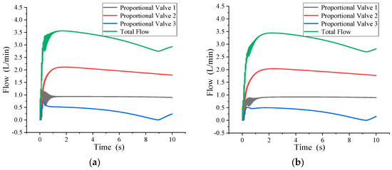
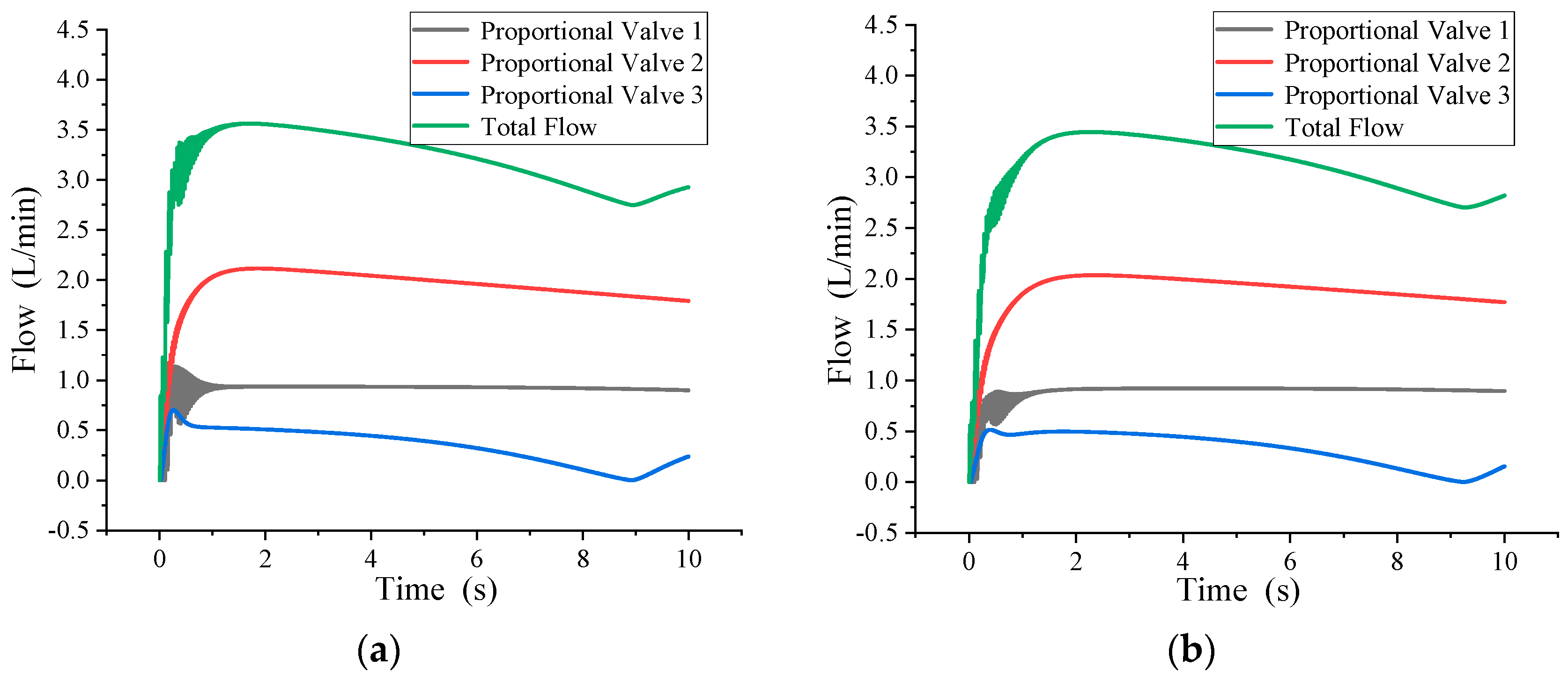
Figure 5 shows the flow curves for multi-joint motion control. It can be seen from the figure that throughout the entire motion control simulation process, the total flow demand of the three joints never exceeds the system’s limit of 15 L/min. From the previous simulation, it is known that when step signals are simultaneously set for all three robotic arm joints, the system experiences insufficient supply flow. To verify the effectiveness of the designed control method when flow demand exceeds the system supply limit, a motion control simulation is performed with step signals simultaneously input to all three hydraulic cylinders.

Figure 5. Multi-joint motion control flow curves: (a) improved deviation coupling control; (b) deviation coupling control.

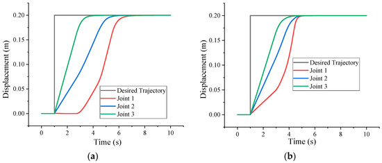
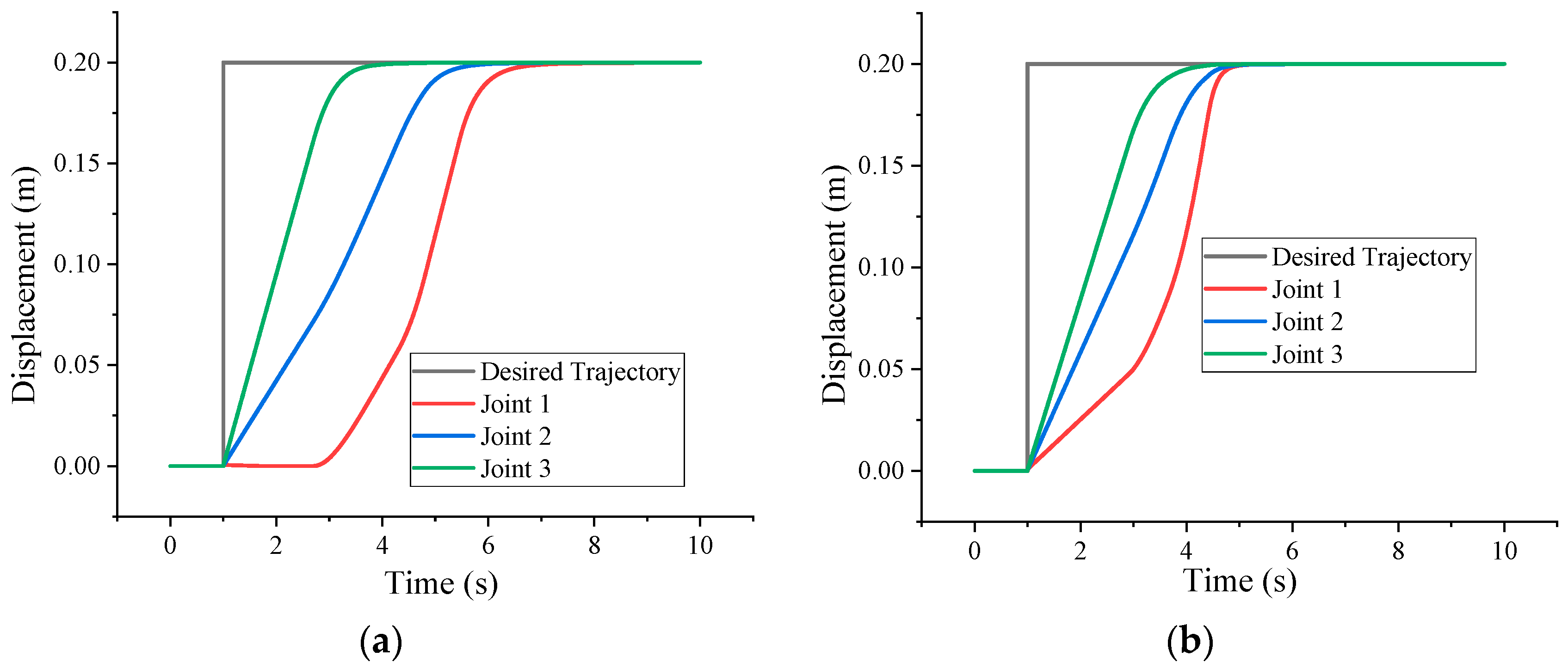
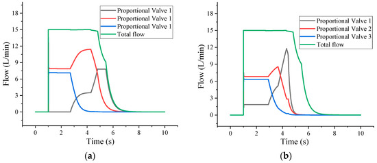
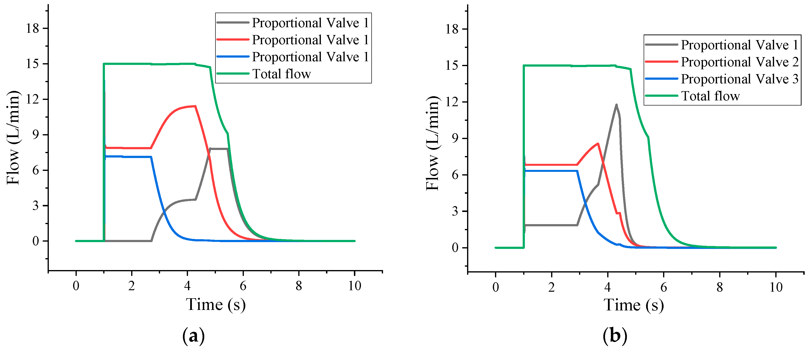
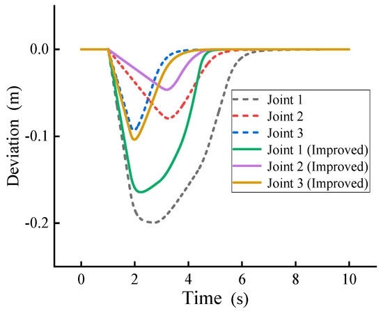
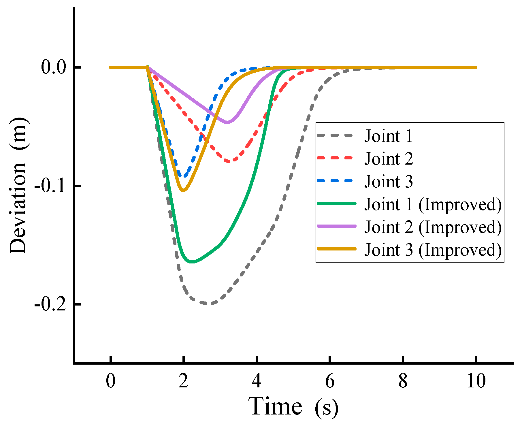
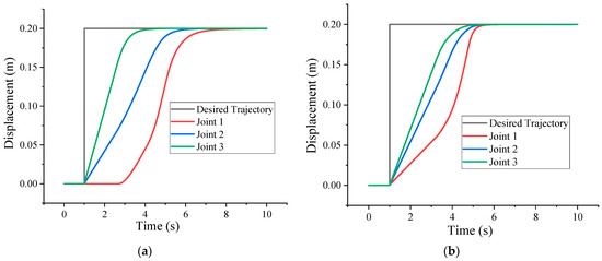
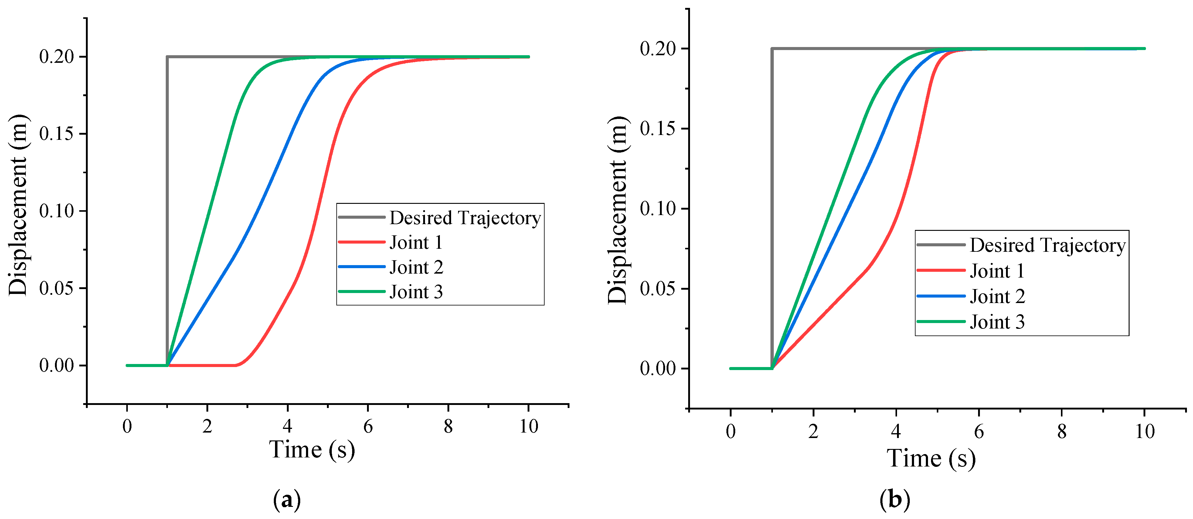
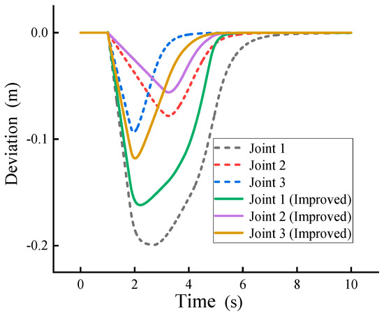
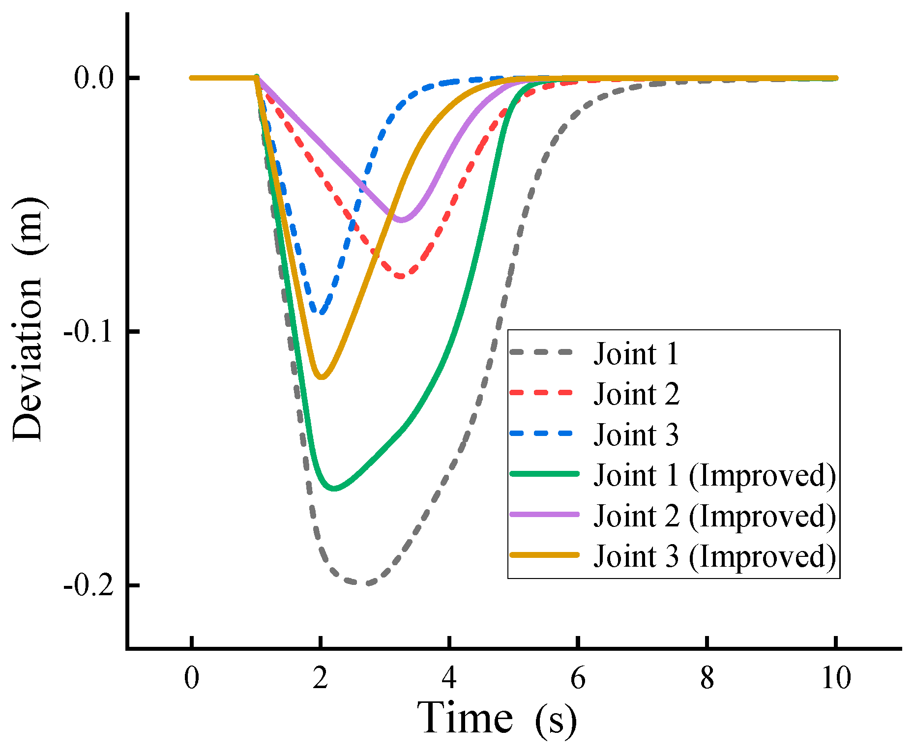
The simulation results for all three hydraulic cylinders using step signals as control signals are shown in Figure 6 and Figure 7. The deviation curve introduced due to joint coupling is shown in Figure 8. From the trajectory curves in Figure 6 and the flow curves in Figure 7, it can be concluded that when using the deviation coupling control method, due to insufficient system flow supply, the control system fails to promptly capture this critical information and make compensations. Joint 1 remains stagnant for a long time. Only when the flow demands of Joints 2 and 3 decrease does Joint 1 receive a portion of the flow and begin to move. Finally, at 6.66 s, all three joints reach their desired positions. When using the improved deviation coupling control method, the system can promptly compensate for Joint 1, avoiding the situation where one joint stagnates due to insufficient flow. The system finally completes the action at 4.8 s, reducing the overall system settling time by 1.86 s, which is a 27.93% reduction compared to the original control method.

Figure 6. Multi-joint motion control trajectory curves with step signal input: (a) deviation coupling control; (b) improved deviation coupling control.

Figure 7. Multi-joint motion control flow curves with step signal input: (a) deviation coupling control; (b) improved deviation coupling control.

Figure 8. Simulation curves of deviation caused by joint coupling.

5. Experimental Verification

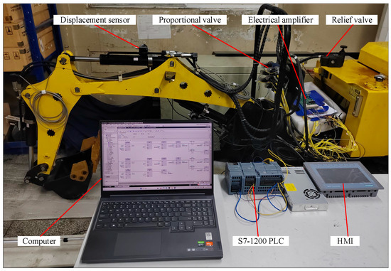
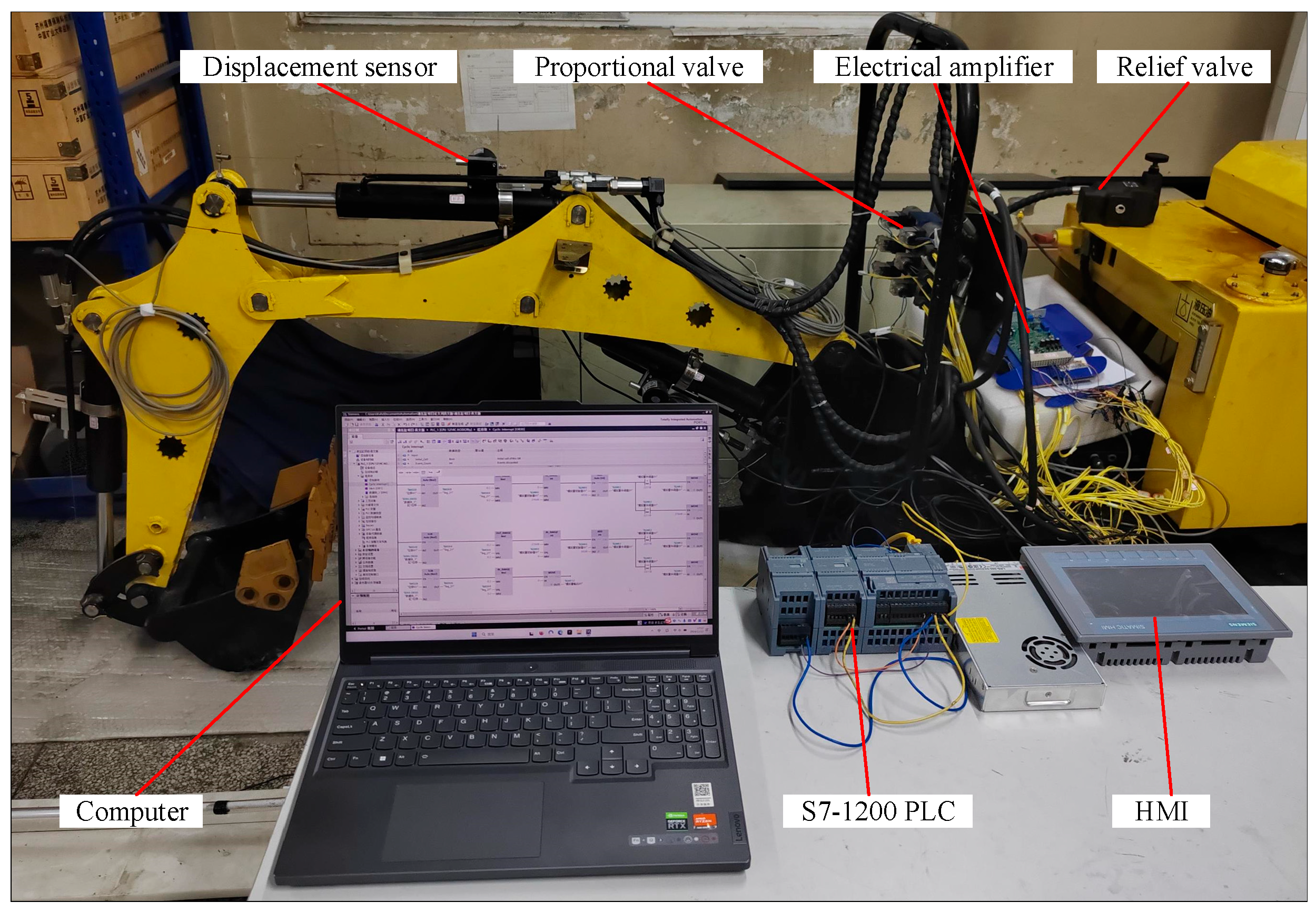
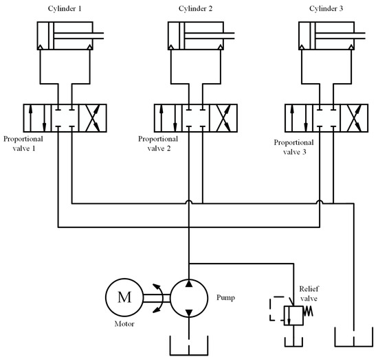
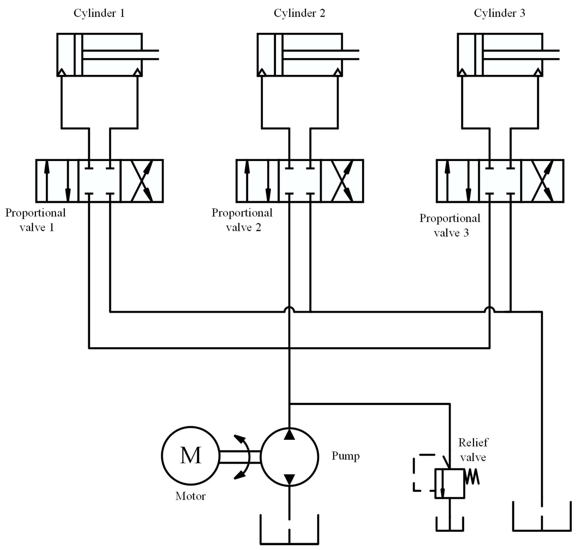
To validate the proposed control method, an experimental platform for an electro-hydraulic proportional control system was developed using the boom cylinder of a compact excavator, as illustrated in Figure 9. The hydraulic circuit of the experimental setup is shown in Figure 10. The three cylinders depicted correspond to the excavator’s boom, bucket, and arm functions. Power was supplied by an electric motor driving a gear pump via coupling, with hydraulic oil directed to the cylinder through a proportional directional valve. The signal control subsystem comprised an upper computer, a Siemens S7-1200 PLC (PLC, manufactured by Siemens AG, Munich, Germany), a signal conditioning board, the proportional directional valve, and a displacement transducer. The displacement transducer captured the real-time position of the cylinder rod, and the signal was fed through the conditioning board and PLC to the upper computer. Based on the acquired displacement data, the upper computer generated a command signal, which was then transmitted to the PLC. The PLC output, after amplification by the signal conditioning board, regulated the spool position of the proportional directional valve, thereby modulating the flow direction and rate of the hydraulic oil to achieve precise extension and retraction of the cylinder.

Figure 9. Small excavator experimental platform.

Figure 10. Hydraulic schematic diagram of excavator.

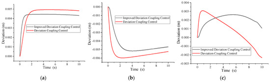
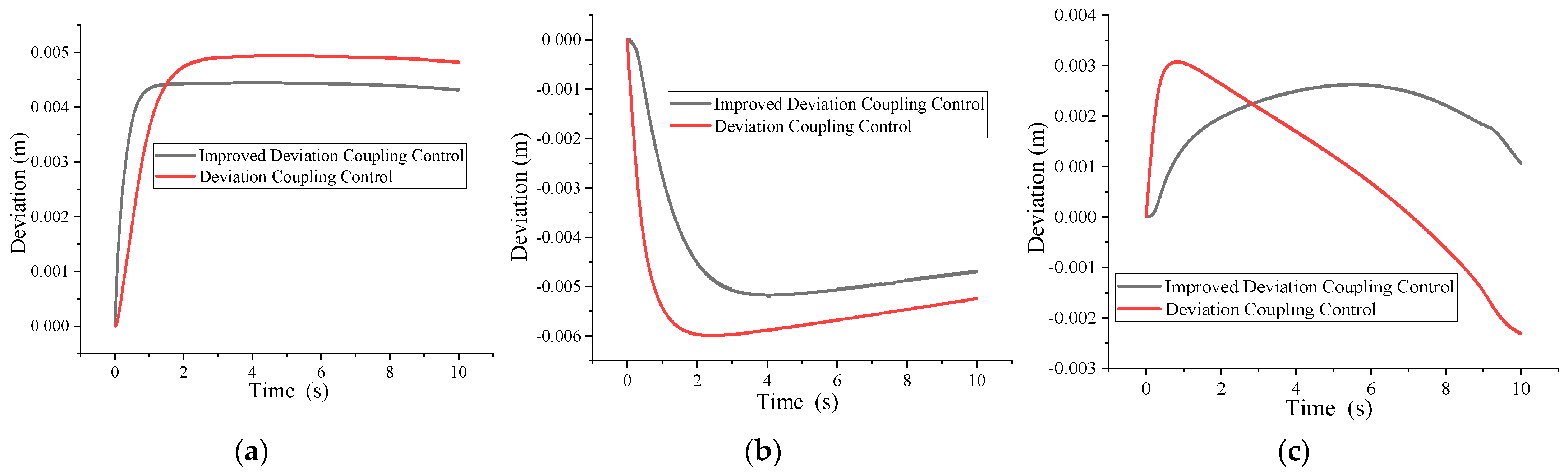
The results of the linear trajectory planning were used as the input signal for the control system. The trajectory curves and deviation curves for the multi-joint motion control experiment are shown in Figure 11 and Figure 12, respectively. For Joint 1 of the robotic arm, when using deviation coupling control in the experiment, the error rises rapidly at the beginning, reaching 4.90 mm at 2.81 s, and then stabilizes around 4.90 mm. Using the improved deviation coupling control, the error also rises at the beginning, reaching 4.40 mm at 1.23 s, and then stabilizes around 4.40 mm. The peak error is reduced by approximately 10.20%. For Joint 2 of the robotic arm, both the original and improved deviation coupling control show a trend of the trajectory deviation first increasing and then decreasing. Using deviation coupling control, the trajectory deviation of Joint 2 reaches its maximum value of 5.99 mm at 2.14 s. Using the improved deviation coupling control, the trajectory deviation of Joint 2 reaches its maximum value of 5.19 mm at 4.02 s. The peak error is reduced by approximately 13.36%. For Joint 3 of the robotic arm, using deviation coupling control, the deviation reaches its maximum value of 3.08 mm at 0.78 s, and the absolute value of the deviation shows an overall trend of first increasing, then decreasing, and then increasing again. Using the improved deviation coupling control, the deviation reaches its maximum value of 2.60 mm at 4.79 s. The peak error is reduced by approximately 15.58%.

Figure 11. Trajectory curves of multi-joint motion control experiment: (a) Joint 1, (b) Joint 2, (c) Joint 3.

Figure 12. Deviation curves of multi-joint motion control experiment: (a) Joint 1, (b) Joint 2, (c) Joint 3.

From the previous simulation, it is known that during linear trajectory tracking, the system’s flow supply can meet the demand. To verify the effectiveness of the control strategy when the system flow supply is insufficient, an experiment was conducted where all three joints simultaneously tracked step signals. The trajectory curves for each joint are shown in Figure 13. The deviation caused by joint coupling is shown in Figure 14. Due to insufficient system flow supply, it can be seen that when using deviation coupling control, after the step input is applied, Joints 2 and 3 begin to move immediately. At 2.68 s, because the flow demands of the other two joints gradually decrease, Joint 1 obtains sufficient flow to drive its motion and begins to move slowly. Finally, Joints 1, 2, and 3 reach their desired positions at 7.35 s, 5.81 s, and 3.94 s, respectively. The settling times for the three joints are 6.35 s, 4.81 s, and 2.94 s, respectively. When using the improved deviation coupling control, after the step input is applied, Joints 1, 2, and 3 can all start moving immediately and finally reach their desired positions at 5.35 s, 5.05 s, and 4.70 s, respectively. The settling times for the three joints are 4.35 s, 4.05 s, and 3.70 s, respectively. Although the settling time for Joint 3 is extended by 0.76 s, the settling times for Joints 1 and 2 are significantly reduced. The overall adjustment time of the robotic arm is reduced from 6.35 s to 4.35 s, a reduction of 2 s, or 31.50%. Therefore, it can be concluded that the improved deviation coupling control strategy is effective.

Figure 13. Experimental trajectory curves of multi-joint motion control under step signal input: (a) deviation coupling control; (b) improved deviation coupling control.

Figure 14. Experimental curves of deviation caused by joint coupling.

The experimental improvements in peak tracking error (10.20–15.58%) are less pronounced than those of the simulation results (up to 49.89%). This discrepancy can be attributed to several factors: (1) the simulation model assumes idealized hydraulic dynamics with constant bulk modulus and perfect flow distribution, while the experimental setup inevitably includes friction, leakage, temperature effects, and valve dead zone nonlinearities; (2) sensor noise and quantization errors in the displacement transducer degrade the feedback signal quality; and (3) controller gains in the experiment were limited by the actuator’s physical constraints to avoid instability, whereas in simulation they could be tuned more aggressively. Despite these differences, the experimental results consistently demonstrate that the proposed IDCC outperforms the traditional DCC, confirming its practical viability.

6. Conclusions

(1) An improved deviation coupling control (IDCC) strategy is proposed for multi-joint hydraulic robotic arms. This strategy integrates feedforward–feedback compensation, synchronous error coupling, and a flow-limiting correction term, and demonstrates superior performance in suppressing inter-joint coupling interference and enhancing trajectory tracking accuracy compared to traditional methods.

(2) Simulation and experimental results validate the effectiveness of the proposed approach. The controller significantly reduces the peak trajectory error by up to 49.89% for the three joints, improves the system’s adaptability under flow-saturation conditions, and decreases the overall adjustment time by 27.93% in simulation and 31.50% in experiments.

(3) This study provides a practical and effective control solution for achieving high-precision trajectory tracking of hydraulic robotic arms in complex and dynamic application scenarios such as intelligent mining. The established coupled dynamic model and the proposed control framework lay a solid foundation for related research and applications in this field.

References

- Onifade, M.; Said, K.O.; Shivute, A.P. Safe mining operations through technological advancement. Process Saf. Environ. Prot. 2023, 175, 251–258. [Google Scholar] [CrossRef] [Scilit]
- Ralston, J.; Reid, D.; Hargrave, C.; Hainsworth, D. Sensing for advancing mining automation capability: A review of underground automation technology development. Int. J. Min. Sci. Technol. 2014, 24, 305–310. [Google Scholar] [CrossRef] [Scilit]
- Mariz, J.L.V.; Badiozamani, M.M.; Peroni, R.L.; de Abreu Silva, R.M. A critical review of bench aggregation and mining cut clustering techniques based on optimization and artificial intelligence to enhance the open-pit mine planning. Eng. Appl. Artif. Intell. 2024, 133, 108334. [Google Scholar] [CrossRef] [Scilit]
- Raza, M.; Karim, A.; Aman, M.; Al-Khasawneh, M.A.; Faheem, M. Global progress towards the Coal: Tracking coal reserves, coal prices, electricity from coal, carbon emissions and coal phase-out. Gondwana Res. 2025, 139, 43–72. [Google Scholar] [CrossRef] [Scilit]
- Peng, S.; Guo, W.; Li, Y. Chinese coal industry and coal mining engineering education. Min. Eng. 2024, 76, 34–38. [Google Scholar]
- Li, D.; Peng, S.; Guo, Y.; Lin, P. Development status and prospect of geological guarantee technology for intelligent coal mining in China. Green Smart Min. Eng. 2024, 1, 433–446. [Google Scholar] [CrossRef] [Scilit]
- Liu, P.; Zhou, H.; Qiao, X.; Zhu, Y. On the relative kinematics and control of dual-arm cutting robots for a coal mine. Actuators 2024, 13, 157. [Google Scholar] [CrossRef] [Scilit]
- Sun, S.; Meng, X.; Xu, X. Research on obstacle-avoidance trajectory planning for drill and anchor materials handling by a mechanical arm on a coal mine drilling and anchoring robot. Sensors 2024, 24, 6866. [Google Scholar] [CrossRef] [Scilit]
- Wang, J.; Huang, Z. The recent technological development of intelligent mining in China. Engineering 2017, 3, 439–444. [Google Scholar] [CrossRef] [Scilit]
- Ghoshal, S.K.; Pandey, A.K.; Dasgupta, K.; Bhola, M. A segmental pump-motor control scheme to attain targeted speed under varying load demand of a hydraulic drive used in heavy earth movers. Mechatronics 2021, 80, 102681. [Google Scholar] [CrossRef] [Scilit]
- Wu, H. Simulation analysis of hydraulic control system of engineering robot arm based on ADAMS. Int. J. Adv. Comput. Sci. Appl. 2023, 14, 414–420. [Google Scholar] [CrossRef] [Scilit]
- Zhong, J.; Jiang, W.; Zhang, Q.; Zhang, W. Design and simulation of a seven-degree-of-freedom hydraulic robot arm. Actuators 2023, 12, 362. [Google Scholar] [CrossRef] [Scilit]
- Guo, Q.; Yu, T.; Jiang, D. Robust H∞ positional control of 2-DOF robotic arm driven by electro-hydraulic servo system. ISA Trans. 2015, 59, 55–64. [Google Scholar] [CrossRef] [Scilit] [PubMed]
- Xu, J.; Sui, Z.; Wei, X. Singular perturbation decoupling and composite control scheme for hydraulically driven flexible robotic arms. Processes 2025, 13, 1805. [Google Scholar] [CrossRef] [Scilit]
- Majstorovic, V.; Simeunovic, V.; Miskovic, Z.; Mitrovic, R.; Stosic, D.; Dimitrijevic, S. Smart manufacturing as a framework for smart mining. Procedia CIRP 2021, 104, 188–193. [Google Scholar] [CrossRef] [Scilit]
- Wang, G.; Pang, Y.; Ren, H.; Zhan, K.; Du, M.; Zhang, Y.; Cheng, J.; Du, Y.; Zhang, J.; Gong, S.; et al. System engineering and key technologies research and practice of smart mine. J. China Coal Soc. 2024, 49, 181–202. [Google Scholar]
- Ren, Z.; Chen, J.; Miao, Y.; Miao, Y.; Guo, Z.; Hu, B.; Lin, R. Adaptive sliding mode control of robotic manipulator based on reinforcement learning. Asian J. Control 2024, 26, 2703–2718. [Google Scholar] [CrossRef] [Scilit]
- Karahan, O.; Karci, H. Design of robust fractional order fuzzy PID sliding mode controller based on hybrid swarm intelligence algorithm for a 6-DOF robotic manipulator. Robotica 2025, 43, 1110–1139. [Google Scholar] [CrossRef] [Scilit]
- Wei, X.; Wangm, Z.; Li, J.; Yin, H. Hybrid neural network adaptive fuzzy sliding mode online compensatory control for robots with global stability. Neurocomputing 2025, 657, 131632. [Google Scholar] [CrossRef] [Scilit]
- Sutyasadi, P.; Wicaksono, M.B. Robotic arm joint position control using iterative learning and mixed sensitivity H∞ robust controller. Bull. Electr. Eng. Inform. 2021, 10, 1864–1873. [Google Scholar] [CrossRef] [Scilit]
- Xue, Y.; Wang, B.; Xu, J.; Sun, Q.; Zhang, P. Research on multi-cylinder coordinated coupling synchronous control strategy based on strain energy. Sci. Rep. 2025, 15, 44277. [Google Scholar] [CrossRef] [Scilit]
- Wos, P.; Dindorf, R. Synchronized trajectory tracking control of 3-DoF hydraulic translational parallel manipulator. Adv. Intell. Syst. Comput. 2015, 317, 269–277. [Google Scholar]
- Lefeber, A.A.J.; Daerden, F.; Vanderborght, B. Coordinated Control of Hydraulic Mobile Manipulators. IFAC Proc. Vol. 2012, 45, 435–440. [Google Scholar] [CrossRef] [Scilit]
- Mu, Y.; Qi, L.; Sun, M.; Han, W. An improved deviation coupling control method for speed synchronization of multi-motor systems. Appl. Sci. 2024, 14, 5300. [Google Scholar] [CrossRef] [Scilit]
- Zhao, W.; Bhola, M.; Ebbesen, M.K.; Andersen, T.O. A novel control design for realizing passive load-holding function on a two-motor-two-pump motor-controlled hydraulic cylinder. Model. Identif. Control 2023, 44, 115–128. [Google Scholar]
- Petrović, G. Mathematical modelling and virtual decomposition control of heavy-duty parallel–serial hydraulic manipulators. Mech. Mach. Theory 2022, 170, 104680. [Google Scholar]
- Bao, Q.; Zhou, J.; Jing, C.; Zhao, H.; Wu, Y.; Zhang, Z. Nonlinear dynamic model for the free rotor of the swash plate-rotating hydraulic transformer. Energy 2022, 261, 125355. [Google Scholar] [CrossRef] [Scilit]
- Guo, X.; Wang, H.; Wang, L.; Liu, H. Adaptive neural network sliding mode control for serially connected hydraulic cylinders of a heavy-duty hydraulic manipulator. J. Mech. Sci. Technol. 2023, 37, 4123–4135. [Google Scholar] [CrossRef] [Scilit]
- Spong, M.W.; Hutchinson, S.; Vidyasagar, M. Robot Modeling and Control, 2nd ed.; Wiley: Hoboken, NJ, USA, 2020. [Google Scholar]
- Manring, N.D.; Fales, R.C. Hydraulic Control Systems, 2nd ed.; Wiley: Hoboken, NJ, USA, 2022. [Google Scholar]
- Habibi, S.; Goldenberg, A. Design of a new high-performance electrohydraulic actuator. IEEE/ASME Trans. Mechatron. 2000, 5, 158–164. [Google Scholar]
- Stosiak, M.; Karpenko, M.; Deptuła, A.; Urbanowicz, K.; Skačkauskas, P.; Cieślicki, R.; Deptuła, A. Modelling and Experimental Verification of the Interaction in a Hydraulic Directional Control Valve Spool Pair. Appl. Sci. 2023, 13, 458. [Google Scholar]
- Xu, B.; Ding, R.; Zhang, J.; Cheng, M.; Sun, T. Analysis and compensation for the cascade dead-zones in the proportional control valve. ISA Trans. 2017, 66, 393–403. [Google Scholar] [CrossRef] [Scilit] [PubMed]
- Ruijgrok, T.W.; Van der Vlist, H. On the Hamiltonian and Lagrangian formulation of classical dynamics for particles with spin. Phys. A Stat. Mech. Its Appl. 1980, 101, 571–580. [Google Scholar] [CrossRef] [Scilit]
- Mucchi, E.; Dalpiaz, G.; Rivola, A. Elastodynamic analysis of a gear pump. Part I: Pressure distribution and gear eccentricity. Mech. Syst. Signal Process. 2010, 24, 2160–2179. [Google Scholar] [CrossRef] [Scilit]
- Kim, S.; Murrenhoff, H. Measurement of Effective Bulk Modulus for Hydraulic Oil at Low Pressure. J. Fluids Eng. 2012, 134, 021201. [Google Scholar] [CrossRef] [Scilit]
Disclaimer/Publisher’s Note: The statements, opinions and data contained in all publications are solely those of the individual author(s) and contributor(s) and not of MDPI and/or the editor(s). MDPI and/or the editor(s) disclaim responsibility for any injury to people or property resulting from any ideas, methods, instructions or products referred to in the content. |
© 2026 by the authors. Licensee MDPI, Basel, Switzerland. This article is an open access article distributed under the terms and conditions of the Creative Commons Attribution (CC BY) license.