A Fault Diagnosis Method for Rolling Bearings Based on Improved Speed Time-Varying Filtering Empirical Mode Decomposition and Adaptive Sine–Cosine Optimization Algorithm

Abstract

As a critical mechanical component, the operational integrity of rolling bearings is essential for equipment safety. However, under strong noise interference, the weak fault features in vibration signals are difficult to extract. To address this issue, a novel fault diagnosis method is proposed in this paper, which integrates an improved speed time-varying filtering empirical mode decomposition (ISTVF-EMD) with an adaptive sine–cosine optimization algorithm (A-SCA), enabling precise and efficient extraction of fault features. The core of the proposed method lies in improving the conventional time-varying filtering empirical mode decomposition (TVF-EMD) by setting a maximum decomposition layer limit, effectively addressing issues of excessive components and low computational efficiency during the decomposition of low signal-to-noise ratio (SNR) signals. Furthermore, a multi-characteristic frequency energy concentration centrality (MCFECC) index is employed as a fitness function to guide A-SCA in adaptively searching for the optimal bandwidth threshold and fitting order parameters of ISTVF-EMD, thereby extracting components with the most enriched fault information. Validated through simulation and multiple test bench cases, the results indicate that the proposed method can not only significantly enhance the fault characteristic frequencies and their harmonics in the envelope spectrum, successfully diagnosing outer race, inner race, and rolling element faults, but also, compared with the original method, ISTVF-EMD substantially reduces the computational time while ensuring or even improving the decomposition quality. The method presented in this paper provides an effective solution for achieving precise and adaptive fault diagnosis of rolling bearings under strong noise interference.

1. Introduction

Rolling bearings are the core components of rotating mechanical systems, capable of altering the motion forms of mechanical structures to achieve efficient rotational motion. They are widely used in various mechanical equipment across fields such as aerospace and aviation, rail transportation, robotics, electric motors, and marine vessels [1]. The operational condition of rolling bearings directly affects the safety and reliability of the entire equipment. Due to the complex and variable working environment, rolling bearings are subjected to long-term alternating loads, making them highly susceptible to failures such as fatigue spalling, pitting, and fractures. These failures can lead to performance degradation or even equipment shutdown. Therefore, conducting efficient research on rolling bearing fault diagnosis is of great significance for ensuring equipment stability and reducing maintenance costs. The collection and analysis of vibration acceleration from rolling bearings is one of the widely used methods for bearing condition monitoring and fault diagnosis [2]. Due to the complexity of the operating environment, the directly collected vibration acceleration signals often contain a significant amount of interfering noise components, making it impossible to directly assess the operational status of the bearing. Therefore, methods such as signal denoising and decomposition need to be applied to reduce the interference from irrelevant noise, thereby enabling effective condition monitoring and fault diagnosis of the bearing.

In recent research, Li et al. [3] proposed an algorithm combining morphological spectral entropy and an enhanced discrete analytical wavelet transform. This method characterizes fault features by calculating the morphological spectral entropy of vibration signals and employs derivative and enhanced discrete analytical wavelet algorithms for decomposition and diagnosis. Experiments demonstrate that it achieves high recognition accuracy for multiple types of faults. Ma et al. [4] proposed a rolling bearing fault feature extraction method based on the Rime-optimized variational mode decomposition. This method adaptively determines the optimal decomposition parameters of VMD through the RIME algorithm and constructs a sensitive feature vector by combining component kurtosis and sample entropy, achieving rapid and accurate identification of different bearing fault states. Hu et al. [5] proposed a rolling bearing fault diagnosis method that combines sine empirical mode decomposition with an improved sparrow search algorithm-optimized kernel extreme learning machine. By employing SEMD to suppress mode mixing and extract fault features, the method demonstrates high diagnostic reliability under both steady and variable operating conditions. Liu et al. [6] enhanced weak fault impulses using an autoregressive model and maximum correlated kurtosis deconvolution. They then separated and extracted homologous fault curves from the time-frequency spectrum via an improved dynamic path-based multi-curve extraction method, thereby achieving precise isolation and diagnosis of multiple roller faults through time-frequency masking and envelope analysis. Wang et al. [7] preprocessed variable-speed vibration signals through order analysis and adaptively screened effective intrinsic mode function components from empirical mode decomposition using a statistical complexity measure. Subsequently, by combining adaptive shift-frequency stochastic resonance technology, they achieved effective enhancement and extraction of unknown fault features under strong background noise. Guo et al. [8] proposed a fault diagnosis method for rolling bearings based on continuous variational mode decomposition and the energy concentration-location accuracy index, effectively achieving the extraction and diagnosis of weak fault features. Experimental verification demonstrated that this method outperforms traditional variational mode decomposition. Sun et al. [9] improved the preprocessing quality of rolling bearing vibration signals via convex-optimized multichannel singular spectrum analysis, preserving fault modal features. They then achieved precise separation of compound faults and assessment of damage severity through frequency-domain and spatial-domain decomposition. Li et al. [10] adaptively selected optimal filter parameters by employing an improved fast kurtogram to process the original vibration signals, and utilized a novel envelope spectrum analysis technique to extract waveform amplitude distribution features from different frequency bands. This method can effectively extract fault features and accurately diagnose fault conditions of bearings.

Ma et al. [11] proposed a fault diagnosis method based on the joint denoising of improved VMD and an adaptive wavelet threshold. An adaptive wavelet threshold function was designed to perform secondary noise reduction and reconstruction on mixed IMFs, significantly enhancing fault feature representation and improving diagnostic accuracy. Liu et al. [12] extracted system resonance frequencies through stochastic subspace identification to guide impulse sparsity measurement of Autogram. This enabled the selection of an optimal demodulation frequency band that simultaneously matched the natural frequency and exhibited high sparsity, thereby achieving bearing fault diagnosis that synergizes physical mechanisms with data characteristics. Tian et al. [13] identified the optimal resonance band containing rich fault information through adaptive resonant demodulation and constructed semantic features independent of signal separation. By measuring the similarity between features and semantics in the mapping space using spatial Euclidean distance, they achieved accurate identification of unknown compound faults under zero-shot conditions. Wu et al. [14] proposed an adaptive optimal demodulation frequency band selection method based on the spectral coherence fault energy factor. This method adaptively optimizes the bandwidth by combining it with a threshold function, ultimately achieving precise fault identification under complex noise through envelope spectrum analysis. Luan et al. [15] proposed a weak fault diagnosis method based on sparrow search algorithm-optimized variational mode decomposition and Shannon entropy-exponential entropy decision. It utilizes SSA-optimized VMD parameters to decompose the signal, screens and reconstructs IMF components to reduce noise, and then applies the Hilbert transform to the reconstructed signal for fault type identification. Li et al. [16] proposed an adaptive residual spectrum amplitude modulation method, which decomposes the signal into multiple narrow bands and performs residual spectrum amplitude modulation. By introducing a fault harmonic-to-noise ratio metric, the method adaptively selects the optimal frequency band rich in fault information, achieving effective enhancement and accurate identification of fault features under strong interference coupling. Chen et al. [17] proposed a clustering-weighted envelope spectrum method for rolling bearing fault diagnosis without requiring prior knowledge. By automatically identifying potential fault characteristic frequencies in each frequency slice of the spectral coherence and performing clustering-weighted integration, it achieved precise localization of discrete fault frequency bands and diagnosis of compound faults. Shang et al. [18] proposed a method for local spectral kurtosis feature extraction based on linear prediction adaptive filtering and an optimized weighted local spectral kurtosis health indicator assessment. This approach effectively extracts weak fault features while enhancing the robustness and adaptive early warning capability of bearing diagnosis.

Based on the aforementioned domestic and international research landscape, it is evident that studies on rolling bearing fault diagnosis aim to achieve more precise and robust fault identification under challenging conditions with strong noise interference. The primary approaches involve preprocessing vibration signals using advanced signal decomposition techniques—such as enhanced discrete analytical wavelet transform, Rime-optimized variational mode decomposition, and sine empirical mode decomposition—to suppress mode mixing and adaptively extract fault features. Subsequently, intelligent optimization algorithms—such as the improved sparrow search algorithm, sparrow search algorithm, and Rime optimization algorithm—or adaptive mechanisms—like the fast kurtogram and spectral coherence fault energy factor—are employed to optimize model parameters or select frequency bands and components rich in fault information. This enhances the representation of weak fault features and improves the accuracy of fault diagnosis. Therefore, this paper conducts research on bearing fault diagnosis methods from the perspectives of signal decomposition and optimization algorithms.

The remainder of the paper is organized as follows: Section 2 elaborates on the signal processing methodologies adopted, including signal decomposition techniques, signal evaluation metrics, and parameter optimization algorithms, on the basis of which a fault diagnosis method capable of adaptively searching for optimal decomposition components is constructed. Section 3 presents the analysis of simulated signals, verifying the accuracy of the proposed signal processing method in extracting features from signals under complex noise interference. Section 4 conducts an analysis of experimental signals, validating the effectiveness of the proposed algorithm on measured data using datasets from multiple test rigs. Section 5 discusses the results obtained, including comparative analysis with existing methods, interpretability of the proposed framework, and its applicability under different operating conditions. Section 6 provides a comprehensive summary of the entire study and draws corresponding conclusions. Section 7 concludes the paper.

2. Methodology

2.1. Improved TVF-EMD Method

TVF-EMD is an adaptive signal decomposition method [19]. Consistent with traditional empirical mode decomposition, it decomposes any complex signal into a series of intrinsic mode functions (IMFs) and a residual component, where each IMF represents an oscillatory mode of a specific scale within the signal. Compared to EMD, TVF-EMD redefines the calculation of the local mean during the decomposition process by employing a time-varying filter instead of the fixed envelope averaging method used in the original EMD. The cutoff frequency of this time-varying filter can vary over time, allowing it to adaptively adjust based on the local characteristics of the signal. This enables more precise separation of components at different scales and effectively suppresses mode mixing. The main core steps of TVF-EMD are as follows:

(1)

The corresponding analytic signal is constructed from the original signal, as shown in the following formula [19].

$$z\left(t\right)=x\left(t\right)+jH\left[x\left(t\right)\right]=A\left(t\right){\mathrm{e}}^{j\phi (t)}$$

(1)

where H[ ] represents the Hilbert transform function, and A(t) denotes the instantaneous amplitude of the analytic signal, as given by the following formula [19].

$$A\left(t\right)=\sqrt{x{\left(t\right)}^2+H{\left[x\left(t\right)\right]}^2}$$

(2)

φ(t) is the instantaneous phase, as shown in the following formula [19].

$$\phi (t)=\arctan \left({\displaystyle \frac{H\left[x\left(t\right)\right]}{x\left(t\right)}}\right)$$

(3)

(2)

The minima and maxima of the instantaneous amplitude of the analytic signal are calculated. Following the EMD decomposition method, the upper envelope β₁(t) and the lower envelope β₂(t) are constructed, and the mean of the sum and the mean of the difference in the envelopes are computed, as shown in the following formula [19].

$$\left\{\begin{array}{c}{\alpha }_1\left(t\right)={\displaystyle \frac{1}{2}}|{\beta }_1\left(t\right)+{\beta }_2\left(t\right)|\\ {\alpha }_2\left(t\right)={\displaystyle \frac{1}{2}}|{\beta }_1\left(t\right)-{\beta }_2\left(t\right)|\end{array}\right.$$

(4)

(3)

Two functions, η₁(t) and η₂(t), are defined to represent the interpolation results of the local maxima and local minima of the signal, respectively. The corresponding expressions are as follows:

$$\left\{\begin{array}{c}{\eta }_1\left(t\right)={\phi }_1^{\prime }\left(t\right)\left[{\alpha }_1{\left(t\right)}^2-{\alpha }_1\left(t\right){\alpha }_2\left(t\right)\right]+{\phi }_2^{\prime }\left(t\right)\left[{\alpha }_2{\left(t\right)}^2-{\alpha }_1\left(t\right){\alpha }_2\left(t\right)\right]\\ {\eta }_2\left(t\right)={\phi }_1^{\prime }\left(t\right)\left[{\alpha }_1{\left(t\right)}^2+{\alpha }_1\left(t\right){\alpha }_2\left(t\right)\right]+{\phi }_2^{\prime }\left(t\right)\left[{\alpha }_2{\left(t\right)}^2+{\alpha }_1\left(t\right){\alpha }_2\left(t\right)\right]\end{array}\right.$$

(5)

In the formula, the derivative of the instantaneous phase yields the instantaneous frequency, which can therefore be rewritten as the expression for the instantaneous frequency as follows:

$$\left\{\begin{array}{c}{\phi }_1^{\prime }\left(t\right)={\displaystyle \frac{{\eta }_1\left(\begin{array}{c}t\end{array}\right)}{2{\alpha }_1{\left(\begin{array}{c}t\end{array}\right)}^2-2{\alpha }_1\left(\begin{array}{c}t\end{array}\right){\alpha }_2\left(\begin{array}{c}t\end{array}\right)}}+{\displaystyle \frac{{\eta }_2\left(\begin{array}{c}t\end{array}\right)}{2{\alpha }_1{\left(\begin{array}{c}t\end{array}\right)}^2+2{\alpha }_1\left(\begin{array}{c}t\end{array}\right){\alpha }_2\left(\begin{array}{c}t\end{array}\right)}}\\ {\phi }_1^{\prime }\left(t\right)={\displaystyle \frac{{\eta }_1\left(\begin{array}{c}t\end{array}\right)}{2{\alpha }_2{\left(\begin{array}{c}t\end{array}\right)}^2-2{\alpha }_1\left(\begin{array}{c}t\end{array}\right){\alpha }_2\left(\begin{array}{c}t\end{array}\right)}}+{\displaystyle \frac{{\eta }_2\left(\begin{array}{c}t\end{array}\right)}{2{\alpha }_2{\left(\begin{array}{c}t\end{array}\right)}^2+2{\alpha }_1\left(\begin{array}{c}t\end{array}\right){\alpha }_2\left(\begin{array}{c}t\end{array}\right)}}\end{array}\right.$$

(6)

(4)

Based on the two instantaneous frequencies, the local cutoff frequency can be further calculated as shown in the following formula:

$${\phi }_{\mathrm{b}}^{\prime }\left(t\right)={\displaystyle \frac{{\phi }_1^{\prime }\left(t\right)+{\phi }_2^{\prime }\left(t\right)}{2}}={\displaystyle \frac{{\eta }_2\left(t\right)-{\eta }_1\left(t\right)}{4{\alpha }_1\left(t\right){\alpha }_2\left(t\right)}}$$

(7)

(5)

Using a B-spline approximation as the time-varying filter, the signal h(t) can be reconstructed based on the local cutoff frequency, with the expression as follows:

$$h\left(t\right)=\cos \left[\int {\phi }_{\mathfrak{b}}^{\prime }\left(t\right)\mathrm{d}t\right]$$

(8)

(6)

The cutoff criterion for the decomposition is calculated. If the bandwidth of the decomposed signal is sufficiently small, further decomposition is stopped. A relative standard is defined to assess whether the cutoff condition is met, as shown in the following formula:

$$\theta \left(t\right)={\displaystyle \frac{B_l\left(t\right)}{{\phi }_a^{\prime }\left(t\right)}}$$

(9)

In the formula, B_l(t) is the Loughlin instantaneous bandwidth, as shown in the following formula:

$$B_l\left(\begin{array}{c}t\end{array}\right)=\sqrt{{\displaystyle \frac{{\alpha }_1^{\prime }{\left(\begin{array}{c}t\end{array}\right)}^2+{\alpha }_2^{\prime }{\left(\begin{array}{c}t\end{array}\right)}^2}{{\alpha }_1{\left(\begin{array}{c}t\end{array}\right)}^2+{\alpha }_2{\left(\begin{array}{c}t\end{array}\right)}^2}}+{\displaystyle \frac{{\alpha }_1{\left(\begin{array}{c}t\end{array}\right)}^2{\alpha }_2{\left(\begin{array}{c}t\end{array}\right)}^2{\left[\begin{array}{c}{\phi }_1^{\prime }\left(\begin{array}{c}t\end{array}\right)-{\phi }_2^{\prime }\left(\begin{array}{c}t\end{array}\right)\end{array}\right]}^2}{{\left[{\alpha }_1{\left(\begin{array}{c}t\end{array}\right)}^2+{\alpha }_2{\left(\begin{array}{c}t\end{array}\right)}^2\right]}^2}}}$$

(10)

${\phi }_{\alpha }^{\prime }\left(t\right)$ is the weighted average instantaneous frequency, as shown in the following formula:

$${\phi }_{\alpha }^{\prime }\left(t\right)={\displaystyle \frac{{\alpha }_1{\left(t\right)}^2{\phi }_1^{\prime }\left(t\right)+{\alpha }_2{\left(t\right)}^2{\phi }_2^{\prime }\left(t\right)}{{\alpha }_1{\left(t\right)}^2+{\alpha }_2{\left(t\right)}^2}}$$

(11)

Given a bandwidth threshold B, if θ(t) is smaller than the threshold, the residual signal can be considered a narrowband signal, and the decomposition can be stopped. Otherwise, the current component is subtracted from the original signal, and steps (1) to (6) are applied to the remaining signal. This process continues until the final residual signal satisfies the decomposition condition in step (6), thereby completing the TVF-EMD decomposition of the signal.

In the original TVF-EMD decomposition method, parameters such as the decomposition cutoff bandwidth threshold, the B-spline fitting order K, and the maximum allowable decomposition level all affect the accuracy and duration of signal decomposition. To investigate the impact of each parameter on the signal decomposition process, a simulated signal from reference [20] is taken as an example for analysis. The expression of the simulated signal is as follows [20].

$$\begin{array}{c}x\left(\begin{array}{c}t\end{array}\right)=\left[\begin{array}{c}0.3+0.3\sin \left(20\pi t\right)\end{array}\right]\cos \left[600\pi t+1.5\sin \left(20\pi t\right)\right]\\ +\left[1+\sin \left(20\pi t\right)\right]\cos \left[300\pi t+0.5\sin \left(10\pi t\right)\right]\\ +\left[0.5+0.5\sin \left(10\pi t\right)\right]\cos \left[100\pi t+0.8\sin \left(10\pi t\right)\right]\end{array}$$

(12)

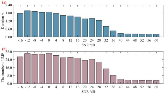
A simulated signal is constructed with a sampling frequency of 10,000 Hz and a duration of 1 s. When performing TVF-EMD decomposition on this signal with a decomposition cutoff bandwidth threshold of 0.1 and a B-spline fitting order of 16 [20], three IMF components without aliasing are obtained [20]. To investigate the decomposition results and efficiency of TVF-EMD under complex noise interference, simulated signals with different signal-to-noise ratios (SNRs) containing mixed Gaussian noise are created. For each SNR, 30 signal realizations are generated, and the decomposition time and the number of IMFs for each SNR are statistically analyzed. The results are shown in Figure 1.

Figure 1. Statistics of TVF-EMD decomposition time and number of IMFs: (a) decomposition time; (b) number of IMFs.

From the statistical results in the figure, it can be seen that the lower the signal-to-noise ratio, the longer the TVF-EMD decomposition takes, and the greater the number of IMFs produced. This leads to more useless components and affects computational efficiency. Measured signals often have low signal-to-noise ratios, which may reduce the decomposition efficiency of the method and diminish its practicality. Therefore, this paper improves the TVF-EMD decomposition method to avoid excessive narrowband IMF components and enhance computational efficiency by imposing a limit on the number of decomposed IMFs. The threshold calculation method is set as shown in the following formula.

$$V_{th}=\left[{\displaystyle \frac{f_s}{W}}\right]$$

(13)

In the formula, f_s is the sampling frequency of the signal, W_b is the defined minimum decomposition bandwidth, and ⌊⋅⌋denotes the floor function. When the number of decomposition levels reaches this threshold, the signal decomposition is stopped.

2.2. Improved Sine–Cosine Optimization Algorithm

The decomposition cutoff bandwidth threshold B and the B-spline fitting order K in TVF-EMD significantly affect the decomposition results of the signal. Therefore, different bandwidth thresholds B and fitting orders K should be selected for different signals. In order to maximally uncover the characteristic information within the signal for effective decomposition, it is necessary to find the optimal bandwidth threshold B and fitting order K. This paper employs the sine–cosine optimization algorithm (SCA) [21] to search for the optimal decomposition result of TVF-EMD under different combinations of B and K, thereby extracting the hidden feature information in the original signal to the greatest extent possible.

The SCA consists of two phases: exploration and exploitation. In the exploration phase, SCA searches for feasible regions across all solutions by incorporating random numbers. In the exploitation phase, random solutions are iteratively refined, updating the position of the optimal solution based on the fluctuation characteristics of the function and combined with random factors [21]. Let X_d represent the search point in the two-dimensional search space formed by the combination of L and M, where d denotes the dimension. The position of the search point is updated as follows:

$$X_d^{j+1}=\left\{\begin{array}{c}{X}_d^j+a{r}_1\sin (r_2)|r_3{P}_d^j-X_d^j|,r_4<0.5\\ X_d^j+a{r}_1\cos (r_2)|r_3{P}_d^j-X_d^j|,r_4\ge 0.5\end{array}\right.,d=1,2$$

(14)

In the formula, j represents the current iteration number; $X_d^j$ denotes the position of the search point in the d-th dimension at the j-th iteration; a is a constant, typically set to 2 [22]; r₁ is the amplitude conversion factor; r₂, r₃, and r₄ are random numbers within the intervals [0, 2π], [0, 2], and [0, 1], respectively; and $P_d^j$ represents the position of the optimal search point at the j-th iteration. The calculation method for the amplitude conversion factor is as follows:

$$r_1=1-{\displaystyle \frac{\mathrm{j}}{\mathrm{J}}}$$

(15)

In the formula, j represents the total number of iterations for the SCA.

The variables searched by the SCA often possess different physical meanings and value ranges. Therefore, it is necessary to set different search ranges and update scales for variables across different dimensions. Based on the original SCA method, this paper modifies the update scales for search points in different dimensions and adopts different values for iteration in each dimension, proposing an adaptive sine–cosine optimization algorithm (A-SCA). The modified search-point position update expression is shown below:

$$X_d^{j+1}=\left\{\begin{array}{c}{X}_d^j+a_d{r}_1\sin (r_2)|r_3{P}_d^j-X_d^j|,r_4<0.5\\ X_d^j+a_d{r}_1\cos (r_2)|r_3{P}_d^j-X_d^j|,r_4\ge 0.5\end{array}\right.,d=1,2$$

(16)

In the formula, a_d is a constant within the d-th dimension, which can take different values according to different dimensions.

Since the B-spline fitting order K must be an integer, it is necessary to ensure that the updated value of K within its corresponding dimensional component remains an integer in each iteration. In this algorithm, the ceiling function is applied to update the value of K during the iterative process.

2.3. Multi-Characteristic Frequency Energy Concentration Centrality Index

The TVF-EMD decomposition often yields multiple components, from which the optimal component must be selected for further analysis to extract signal features. Similarly, optimization algorithms require identifying the best result among multiple outputs, necessitating the establishment of an index for evaluating the richness of signal features. Kurtosis and signal-to-noise ratio (SNR) are commonly used as feature indicators to help identify the optimal decomposed signal. However, in practical applications, kurtosis is susceptible to interference from local outliers. During decomposition, narrowband signals may appear with uneven amplitude distributions and obvious monotonic decay characteristics, leading to abnormally high kurtosis values and potentially biased judgments. While SNR can reflect the level of irrelevant noise in a signal, the original signal is often not captured during data acquisition, making it impossible to calculate the SNR index.

Due to its structural and operational characteristics, rolling bearings often exhibit specific frequency impacts when faults occur. Common bearing fault characteristic frequencies include the outer race fault characteristic frequency, inner race fault characteristic frequency, rolling element fault characteristic frequency, and cage fault characteristic frequency. In bearing fault diagnosis, it is often necessary to analyze the envelope spectrum of vibration acceleration to observe whether distinct characteristic frequencies and their higher-order harmonic spectral lines are present. These are used to determine the type of bearing fault. The more prominent the spectral lines, the more evident the fault features in the signal. Parameters such as CFIC [23,24] can represent this characteristic. However, the CFIC indicator requires prior knowledge of the bearing fault type, which limits its applicability for bearings with undetermined fault types. Therefore, by integrating CFIC and the CFECC indicator [25], this paper establishes a new multi-characteristic frequency energy concentration centrality (MCFECC) index to identify the frequency component with the most concentrated energy among multiple specific frequencies. The CFECC indicator mentioned in reference [26] is shown below:

$$\left\{\begin{array}{c}\begin{array}{l}EC{C}_{mt}={\displaystyle \sum _{i=1}^P}{\displaystyle \frac{E_{\max }\left(\left[\left(1-r\right)f_t,\left(1+r\right)f_t\right]\right)·\left(L-1\right)}{\sum E\left(\left[\left(1-r\right)f_t,\left(1+r\right)f_t\right]\right)-E_{\max }\left(\left[\left(1-r\right)f_t,\left(1+r\right)f_t\right]\right)}}\\ EC{C}_{lt}={\displaystyle \sum _{i=1}^P}{\displaystyle \frac{E_{\max }\left(\left[\left(1-2r\right)f_t,\left(1-r\right)f_t\right]\right)·\left(L-1\right)}{\sum E\left(\left[\left(1-2r\right)f_t,\left(1-r\right)f_t\right]\right)-E_{\max }\left(\left[\left(1-2r\right)f_t,\left(1-r\right)f_t\right]\right)}}\end{array}\\ \begin{array}{l}EC{C}_{rt}={\displaystyle \sum _{i=1}^P}{\displaystyle \frac{E_{\max }\left(\left[\left(1+r\right)f_t,\left(1+2r\right)f_t\right]\right)·\left(L-1\right)}{\sum E\left(\left[\left(1+r\right)f_t,\left(1+2r\right)f_t\right]\right)-E_{\max }\left(\left[\left(1+r\right)f_t,\left(1+2r\right)f_t\right]\right)}}\\ CFEC{C}_t={\displaystyle \frac{2EC{C}_{mt}}{P\left(EC{C}_{lt}+EC{C}_{rt}\right)}}\end{array}\end{array}\right.$$

(17)

In the formula, P is the selectable harmonic order of the characteristic frequency, $E_{\max }\left(\left[\left(1-r\right)f_t,\left(1+r\right)f_t\right]\right)$ is the maximum amplitude energy within the envelope spectrum interval $\left[\left(1-r\right)f_t,\left(1+r\right)f_t\right]$, ${\displaystyle \sum E\left(\left[\left(1-r\right)f_t,\left(1+r\right)f_t\right]\right)}$ is the sum of the amplitude values at all frequencies within that interval, L is the number of discrete frequency points of the spectrum in that interval, f_t is the selected characteristic frequency, and r is the relative error range of the characteristic frequency.

To rapidly identify fault characteristic information, based on Equation (17) and incorporating different fault characteristic frequencies of the bearing, the CFECC parameters corresponding to multiple fault characteristic frequencies of the bearing are calculated simultaneously. The largest parameter among them is selected as the final characteristic indicator, MCFECC. The calculation method is as follows:

$$MCFECC=\max \left(CFEC{C}_o,CFEC{C}_i,CFEC{C}_r,CFEC{C}_c\right)$$

(18)

In the formula, CFECC_o represents the characteristic indicator for the bearing outer race fault frequency, CFECC_i represents the characteristic indicator for the bearing inner race fault frequency, CFECC_r represents the characteristic indicator for the bearing rolling element fault frequency, and CFECC_c represents the characteristic indicator for the bearing cage fault frequency. The function max() denotes selecting the maximum value.

2.4. Framework of the Proposed Fault Diagnosis Method

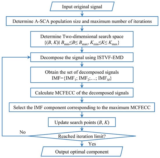
Based on the analysis and introduction above, this paper proposes a bearing fault diagnosis algorithm based on improved TVF-EMD and sine–cosine optimization. By establishing a mapping relationship between MCFECC and the bandwidth threshold B and fitting order K of ISTVF-EMD, which serves as the fitness function for SCA, the optimal bandwidth threshold B and fitting order K are sought to decompose the signal under analysis. Subsequently, fault feature information is extracted from the optimal decomposition component through envelope spectrum analysis. The flowchart of the fault diagnosis method is shown in Figure 2.

Figure 2. Flowchart of the fault diagnosis method.

Step 1: Input the original signal and initialize the population size and maximum number of iterations for A-SCA.

Step 2: Define the ranges of parameters B and K optimized by A-SCA.

Step 3: The signal is decomposed using ISTVF-EMD, and the respective IMF components are obtained.

Step 4: Calculate the MCFECC eigenvalue of each IMF component.

Step 5: Select the IMF component corresponding to the maximum MCFECC as the optimal component for this iteration, update the values of B and K, and proceed to the next iterative calculation.

Step 6: Perform Hilbert demodulation on the finally determined optimal component to extract fault characteristic frequency information.

3. Simulation Data Analysis

To verify the effectiveness of the proposed rolling bearing fault diagnosis method, numerical simulation signals with known fault characteristic frequencies are established for algorithm analysis and validation.

3.1. Simulation Signal Model

Due to the periodic motion of the rolling elements, when various components of a rolling bearing develop faults, a series of periodic impacts is generated. Owing to machining errors and the local distribution of the load zone, the impact period of bearing faults often exhibits slight fluctuations. Therefore, when establishing a numerical simulation signal model, it is generally necessary to introduce random variations to represent this stochastic impact characteristic of the bearing [26]. With reference to the numerical signal models in the literature [25,26], the expression for the faulty bearing numerical simulation signal model used in this paper is established as follows:

$$y\left(t\right)=\sum _{i=1}^{435}{\mathrm{e}}^{-450\left(t-{\displaystyle \frac{i}{121}}-{\tau }_i\right)}·\sin \left[5000\pi \left(t-{\displaystyle \frac{i}{121}}-{\tau }_i\right)\right]+w\left(t\right)$$

(19)

In the formula, ${\tau }_i$ represents the timing error arising from the relative motion among internal bearing components, typically set at 1% to 2% of the fault period; w(t) denotes the environmental noise, which can be modeled as Gaussian white noise to serve as the background noise.

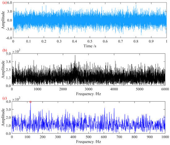
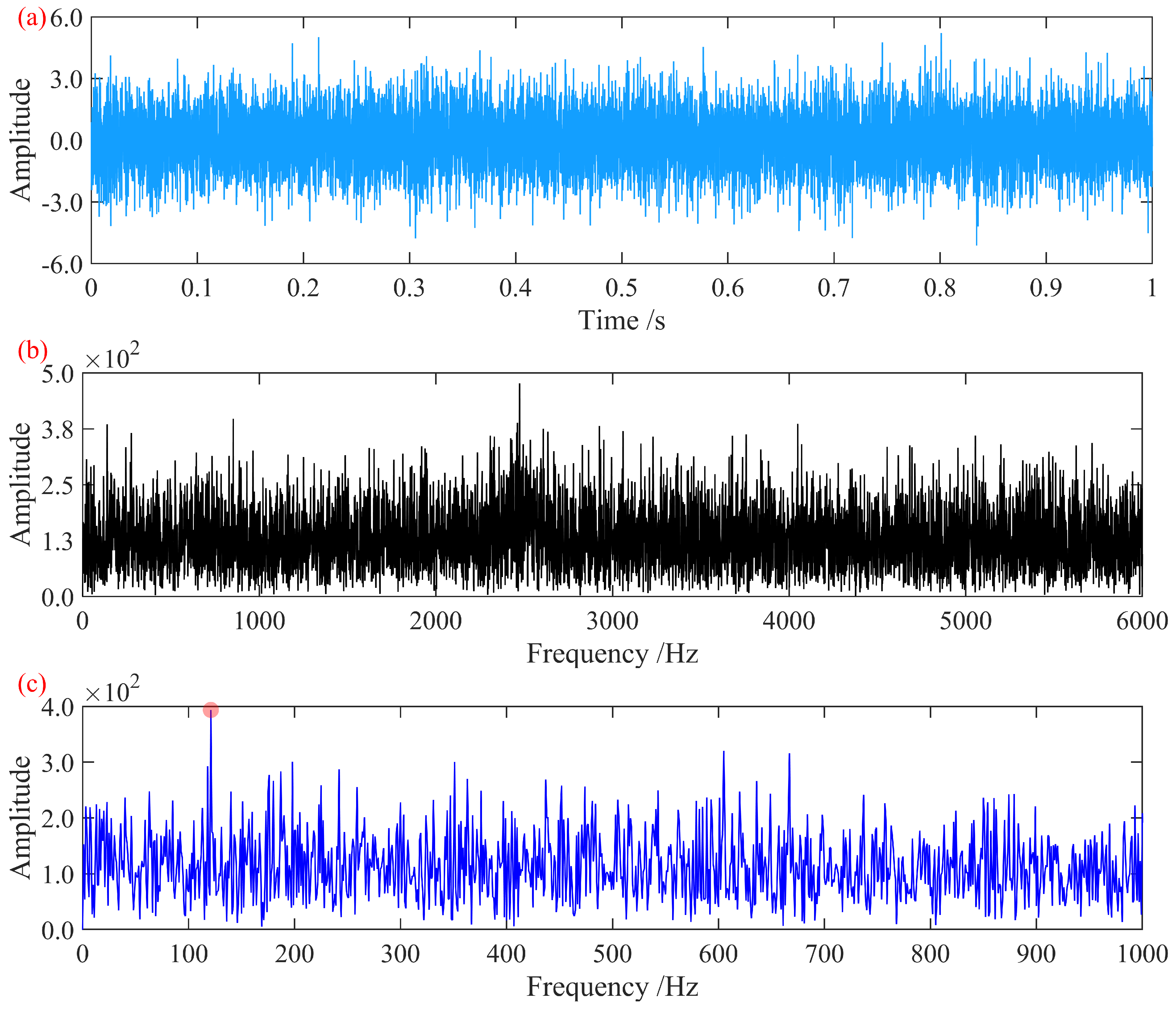
With a sampling frequency of 12,000 Hz, a simulation signal with a duration of 1 s and a signal-to-noise ratio of −13 dB is constructed. Its time-domain diagram and frequency spectrum are shown in Figure 3:

Figure 3. Original simulated signal diagrams: (a) time-domain diagram; (b) frequency-domain diagram; (c) Hilbert envelope spectrum.

3.2. Simulation Results and Analysis

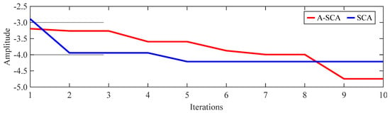
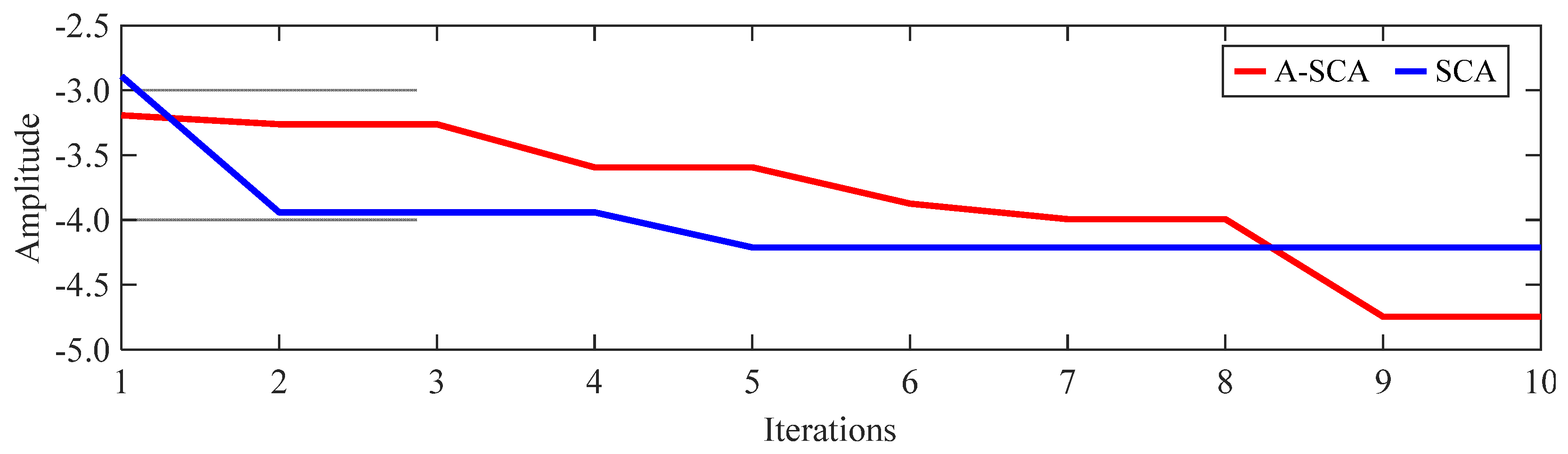
The constructed simulation signal is analyzed and processed. Multiple preset fault characteristic frequencies of 121 Hz, 75 Hz, 157 Hz, and 169 Hz are set, and the MCFECC eigenvalue for each iteration of the signal is calculated. In the MCFECC eigenvalue calculation, P is set to five, and r is set to 0.03. In the A-SCA, the population size is set to 10, the maximum number of iterations is set to 10, the search range for the bandwidth threshold B is set to [0.01, 0.9], and the search range for the fitting order K is set to [5, 30]. Using the negative value of the MCFECC eigenvalue as the search metric, the B and K corresponding to the minimum value are taken as the construction parameters for ISTVF-EMD to decompose the signal. To verify the convergence effectiveness of the A-SCA compared to the SCA, the SCA optimization is also performed on the same signal, with all other algorithm parameters being the same as those of the proposed method. The comparison of the optimization processes between A-SCA and SCA is shown in Figure 4.

Figure 4. Iteration curves of the feature indicator.

Based on the final iterative results of A-SCA, the optimal bandwidth threshold B for ISTVF-EMD is determined to be 0.29613, and the optimal fitting order K is determined to be nine. The signal corresponding to the optimally decomposed component obtained is shown in Figure 5.

Figure 5. A-SCA optimal decomposition signal diagrams: (a) time-domain diagram; (b) frequency-domain diagram; (c) Hilbert envelope spectrum.

In the Hilbert envelope spectrum shown in the figure, a distinct fault characteristic frequency of 121 Hz and its first five harmonics are clearly observed. This effectively represents the fault characteristic information, enabling the extraction and diagnosis of the fault.

Furthermore, based on the final iteration results of the standard SCA, the optimal bandwidth threshold B for ISTVF-EMD was determined to be 0.18489, and the optimal fitting order K was determined to be eight. The resulting optimal decomposition component signal is shown in Figure 6.

Figure 6. Signal decomposed using the optimal parameters from SCA: (a) time-domain waveform; (b) frequency spectrum; (c) Hilbert envelope spectrum.

Compared with Figure 5, the envelope spectrum of the optimal decomposition signal in Figure 6 shows prominent amplitudes only for the first three harmonics of the fault characteristic frequency, while the remaining harmonics are obscured. This comparison demonstrates the superiority of the A-SCA optimization over the standard SCA optimization and verifies the effectiveness of the proposed fault diagnosis algorithm.

4. Experimental Data Analysis

To evaluate the effectiveness of the proposed method for different measured signals, data from the bogie axle-box bearing test rig at Southwest Jiaotong University and signals from the bearing test rig at Xi’an Jiaotong University were analyzed.

4.1. Analysis of Data from the Southwest Jiaotong University Axle-Box Bearing Test Rig

Data from the outer race fault and rolling element fault datasets of the high-speed train axle-box bearing test rig at Southwest Jiaotong University [2,25] are adopted for analysis and validation.

The test rig consists of a three-phase AC induction motor (model YVF160M-4) (Shanxi Electric Motor Manufacturing Co., Ltd., Taiyuan, China), rated power: 11 kW, rated speed: 1460 r/min, a hydraulic vertical loading system, and a vibration excitation platform to simulate track irregularity.

The platform supports rotational speed variation (500–1500 r/min), adjustable static vertical load, and adjustable excitation frequency.

The axle-box bearing test rig adjusts the motor speed by regulating the output power of the frequency converter, thereby controlling the input power to the traction frequency conversion motor. The motor drives the transmission shaft, which is connected via bolts to a universal coupling, subsequently driving the driven main shaft and the inner ring of the test bearing.

Two experimental conditions were configured using this test rig, as shown in Table 1.

Table 1. Experimental conditions.

Test Number	Bearing Type	Fault Type	Bearing Speed	Sampling Frequency
Case 1	Double row tapered roller bearing	Outer race fault	900 r/min	25,600 Hz
Case 2	Double row cylindrical roller bearings	Rolling element fault	1400 r/min	25,600 Hz

4.1.1. Case 1

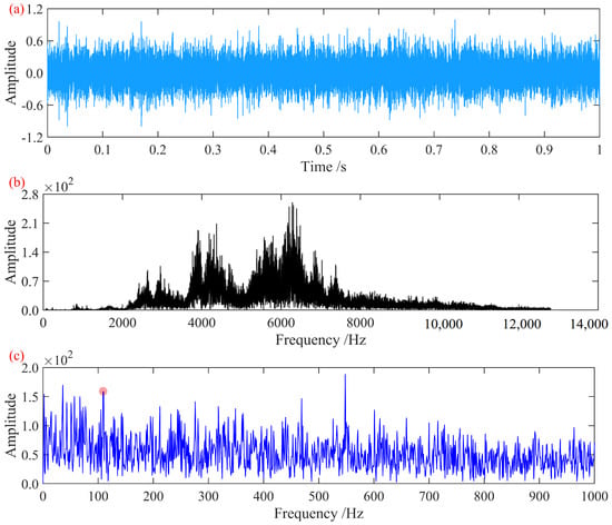
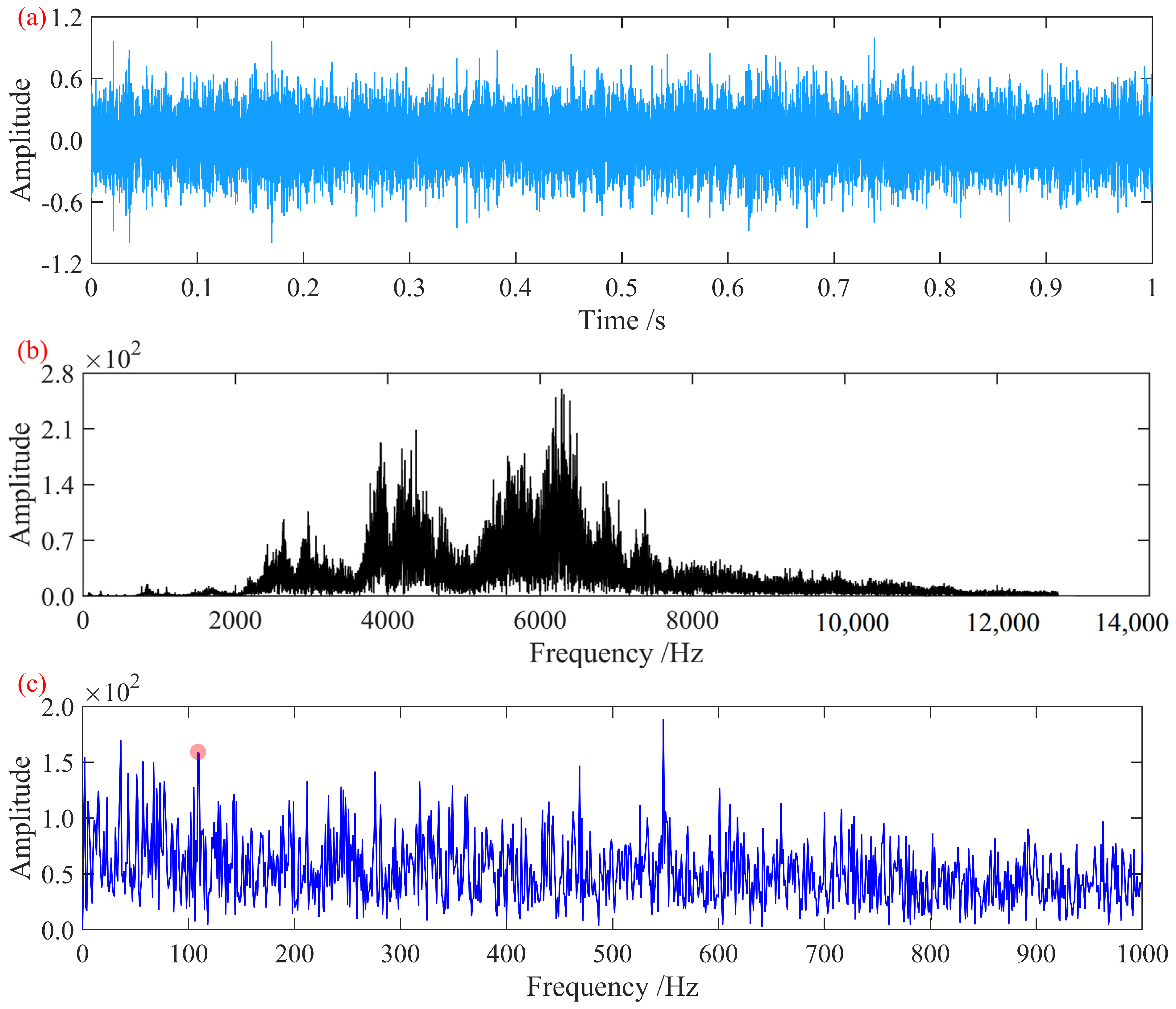
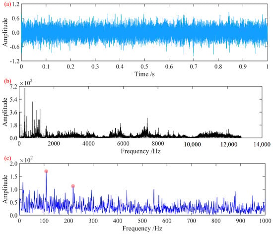
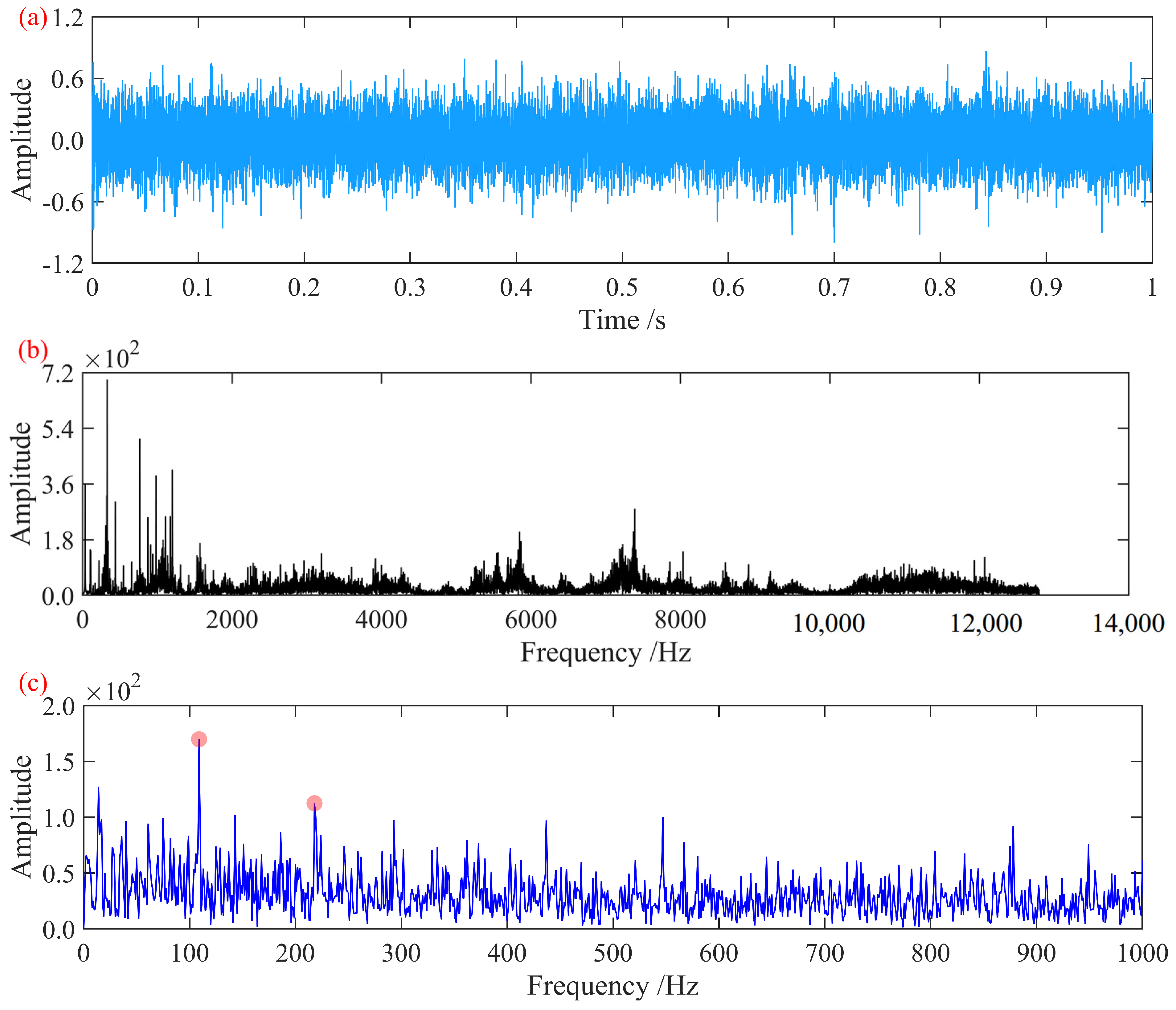
The vibration acceleration signal of the axle-box bearing with an outer race fault in Case 1 was analyzed and processed. At this rotational speed, the characteristic fault frequencies of the axle-box bearing were determined to be outer race fault frequency, 110.56 Hz; inner race fault frequency, 144.44 Hz; rolling element fault frequency, 54.23 Hz; and cage fault frequency, 6.5 Hz. The time-domain waveform and frequency spectrum of the signal, normalized to its maximum amplitude, are shown in Figure 7.

Figure 7. Signal from the axle-box bearing with an outer race fault: (a) time-domain waveform; (b) frequency spectrum; (c) Hilbert envelope spectrum.

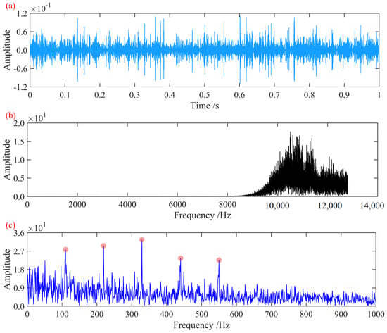
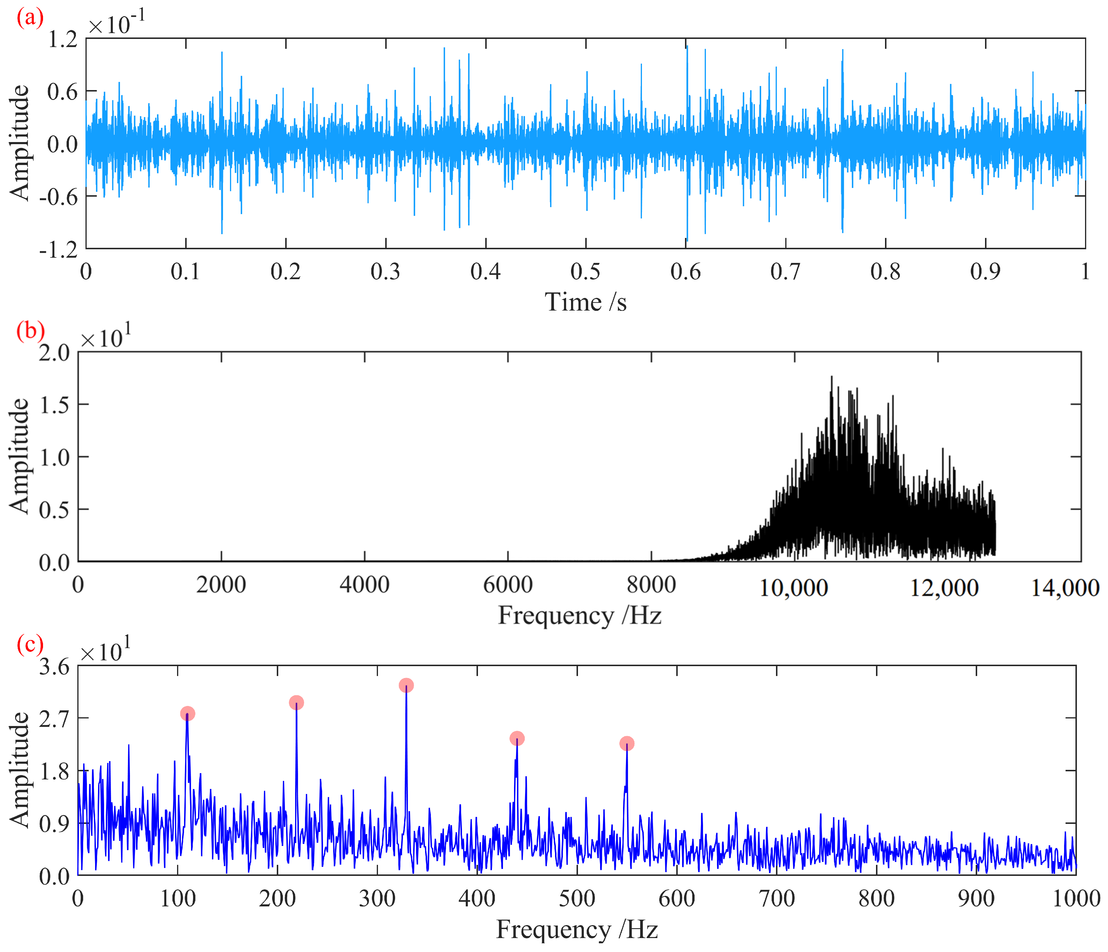
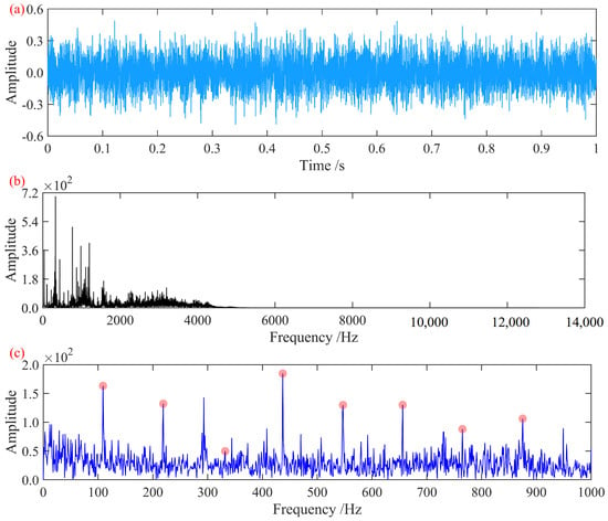
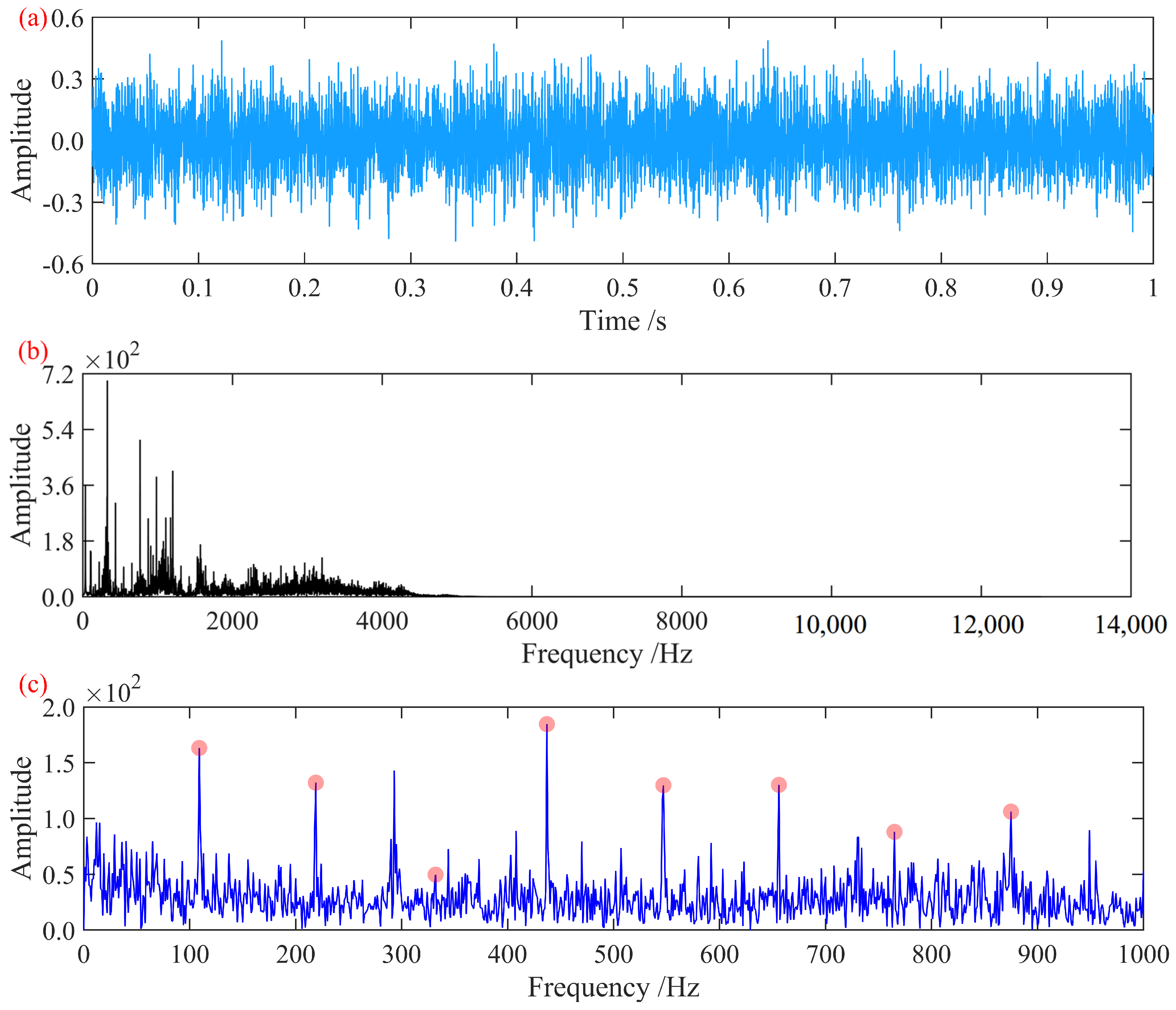
In the Hilbert envelope spectrum of the original signal, only a faintly identifiable first-order fault characteristic frequency is present, while the remaining harmonic features are masked by noise. To extract the hidden fault features, the method proposed in this paper was employed for fault feature extraction. In the process, for the MCFECC eigenvalue, P was set to five, and r was set to 0.03. In the A-SCA, the population size was set to 10, the maximum number of iterations was set to 10, the search range for the bandwidth threshold B was set to [0.05, 0.5], and the search range for the fitting order K was set to [20, 30]. Using the negative value of the MCFECC eigenvalue as the search metric, the B and K corresponding to the minimum value were taken as the construction parameters of ISTVF-EMD to decompose the signal. Through A-SCA iteration, the optimal bandwidth threshold B for ISTVF-EMD was determined to be 0.055403, and the optimal fitting order K was determined to be 20. The optimally decomposed component signal obtained is shown in Figure 8.

Figure 8. Optimal decomposition signal: (a) time-domain waveform; (b) frequency spectrum; (c) Hilbert envelope spectrum.

In the Hilbert envelope spectrum shown in the figure, distinct first-order fault characteristic frequencies at 110 Hz and the first five harmonics are observed, effectively enhancing the hidden outer race fault features in the signal. This demonstrates that the proposed method successfully enhances and extracts the fault characteristics.

4.1.2. Case 2

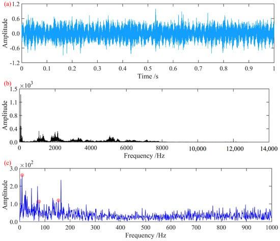
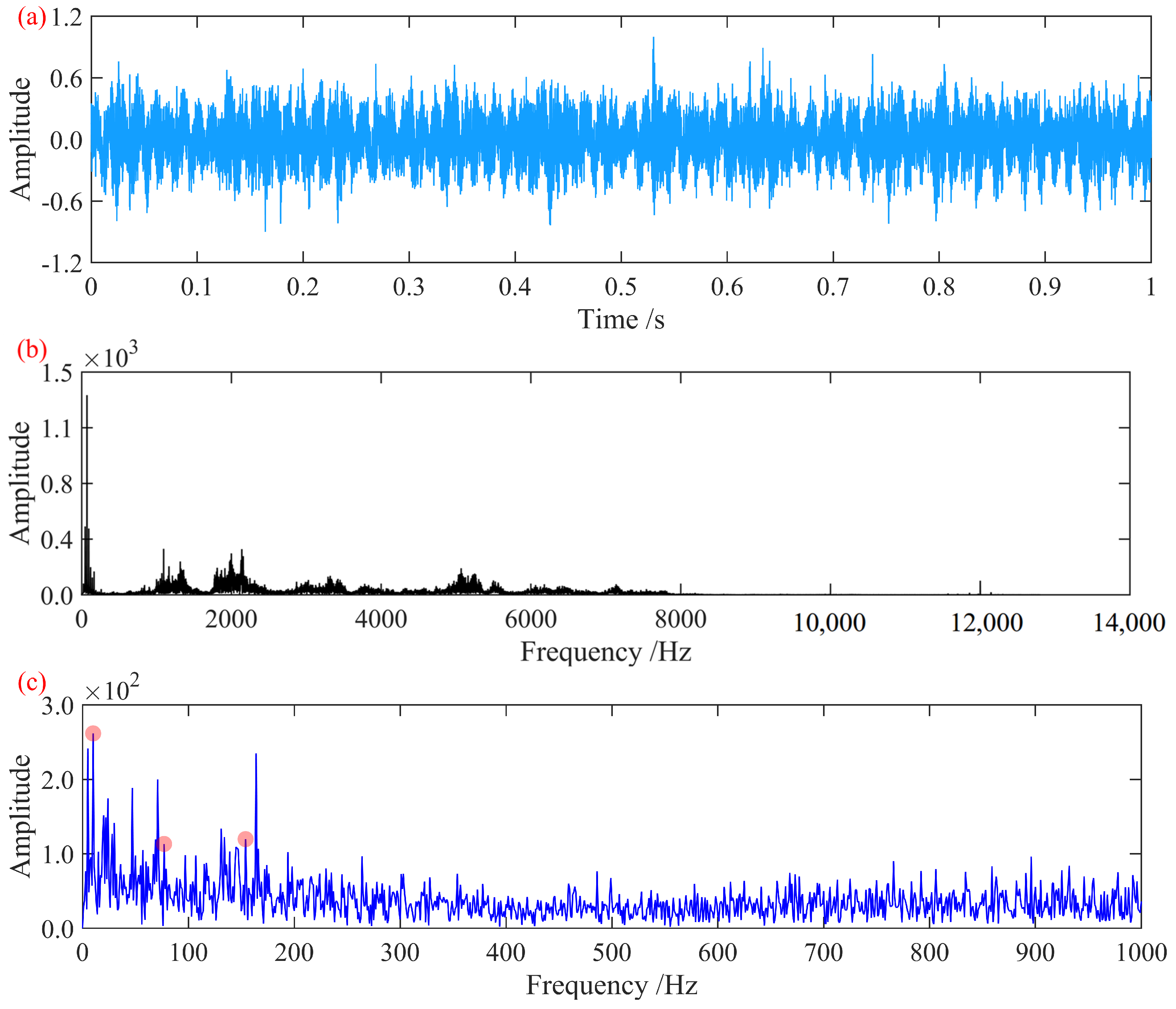
The vibration acceleration signal of the axle-box bearing with a rolling element fault in Case 2 was analyzed and processed. At this rotational speed, the characteristic fault frequencies of the axle-box bearing were determined to be outer race fault frequency, 169.58 Hz; inner race fault frequency, 227.09 Hz; rolling element fault frequency, 78.76 Hz; and cage fault frequency, 9.97 Hz. The time-domain waveform and frequency spectrum of the signal, normalized to its maximum amplitude, are shown in Figure 9.

Figure 9. Signal from the axle-box bearing with a rolling element fault: (a) time-domain waveform; (b) frequency spectrum; (c) Hilbert envelope spectrum.

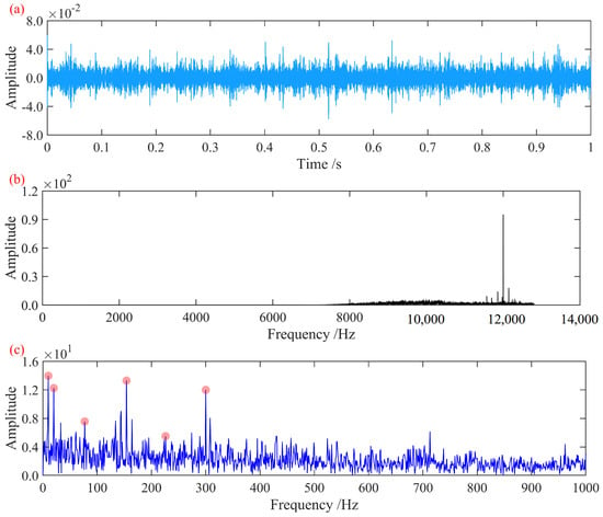
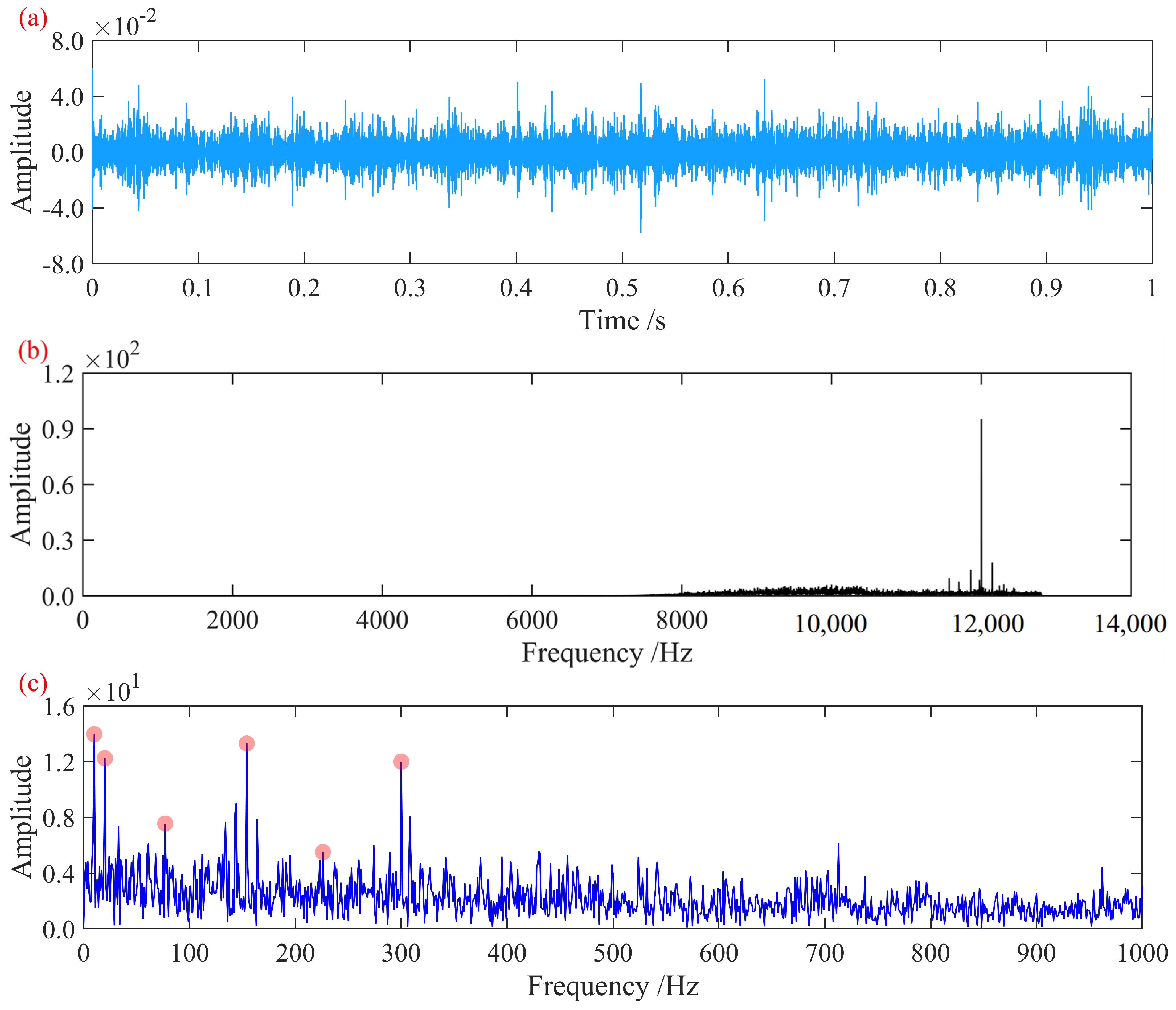
In the Hilbert envelope spectrum of the original signal, only the first-order cage characteristic frequency is present. Since rolling element faults can induce modulation at the cage frequency [26], harmonics at both the cage frequency and the corresponding rolling element fault frequency can be considered indicative of rolling element fault information [26]. However, the primary fault characteristic information—the rolling element characteristic frequency and its harmonics—is masked by noise. The proposed method was applied for fault feature extraction. In the MCFECC feature calculation, parameter P was again set to five and r to 0.03. For the A-SCA, the population size was set to 10, the maximum number of iterations to 10, the search range for the bandwidth threshold B to [0.02, 0.9], and the search range for the fitting order K to [20, 30]. The negative value of the MCFECC feature was used as the search criterion to find the optimal B and K corresponding to the minimum, which were then used as the construction parameters for ISTVF-EMD to decompose the signal. Based on the final A-SCA iteration results, the optimal bandwidth threshold B for ISTVF-EMD was determined to be 0.03526, and the optimal fitting order K was determined to be 27. The resulting optimal decomposition component signal is shown in Figure 10.

Figure 10. Optimal decomposition signal: (a) time-domain waveform; (b) frequency spectrum; (c) Hilbert envelope spectrum.

In the Hilbert envelope spectrum shown in the figure, distinct cage characteristic frequencies and their second harmonics are observed. Simultaneously, the first four fault characteristic frequencies of the rolling elements are clearly present. Cage modulation frequencies are identified at the second and fourth harmonics, where the harmonic amplitudes are notably prominent. This observation is consistent with the conclusion that rolling element faults excite second harmonics due to dual-point contact with both the inner and outer races [26], thereby demonstrating the effectiveness of the proposed fault diagnosis method in identifying bearing rolling element fault characteristic information.

4.2. Analysis of Data from the Xi’an Jiaotong University Bearing Test Rig

To further validate the effectiveness of the method, bearing outer race fault data and inner race fault data from the Xi’an Jiaotong University rolling bearing accelerated life test open dataset [27] were adopted for analysis and validation. The signal sampling frequency is 25.6 kHz.

The dataset contains full run-to-failure vibration signals of 15 rolling element bearings acquired under accelerated degradation experiments. The key bearing parameters are outer race diameter: 39.80 mm; inner race diameter: 29.30 mm; mean diameter: 34.55 mm; ball diameter: 7.92 mm; number of balls: eight; contact angle: 0°; static load rating: 6.65 kN; dynamic load rating: 12.82 kN. The vibration signals include horizontal and vertical acceleration components recorded throughout the degradation process until failure. This dataset provides long-term degradation information under controlled laboratory conditions, making it suitable for evaluating the sensitivity of the proposed decomposition and feature enhancement strategy.

Two datasets representing different fault types were selected. The experimental conditions and data identifiers are summarized in Table 2.

Table 2. Experimental conditions.

Test Number	Bearing Dataset	Fault Type	Bearing Rotational Frequency	Sample Number	Sampling Frequency
Case 3	Bearing1_3	Outer race fault	35 Hz	60	25,600 Hz
Case 4	Bearing2_1	Inner race fault	37.5 Hz	453	25,600 Hz

4.2.1. Case 3

The vibration acceleration signal of the axle-box bearing with an outer race fault in Case 3 was analyzed and processed. At this rotational speed, the characteristic fault frequencies of the axle-box bearing were determined to be outer race fault frequency, 107.9 Hz; inner race fault frequency, 172.1 Hz; rolling element fault frequency, 72.3 Hz; and cage fault frequency, 13.5 Hz. The time-domain waveform and frequency spectrum of the signal, normalized to its maximum amplitude, are shown in Figure 11.

Figure 11. Signal from the bearing with an outer race fault: (a) time-domain waveform; (b) frequency spectrum; (c) Hilbert envelope spectrum.

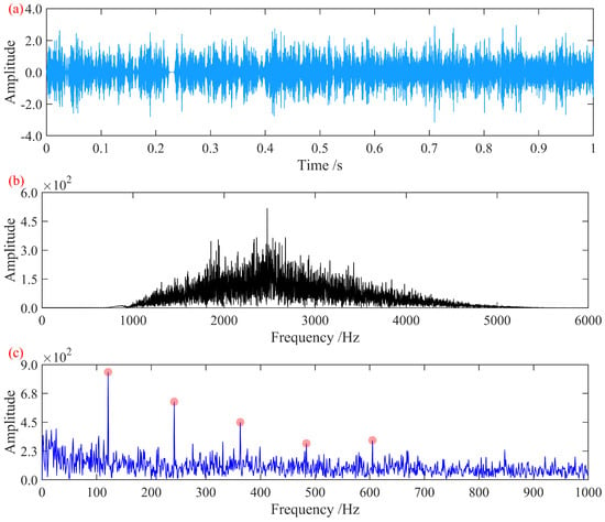
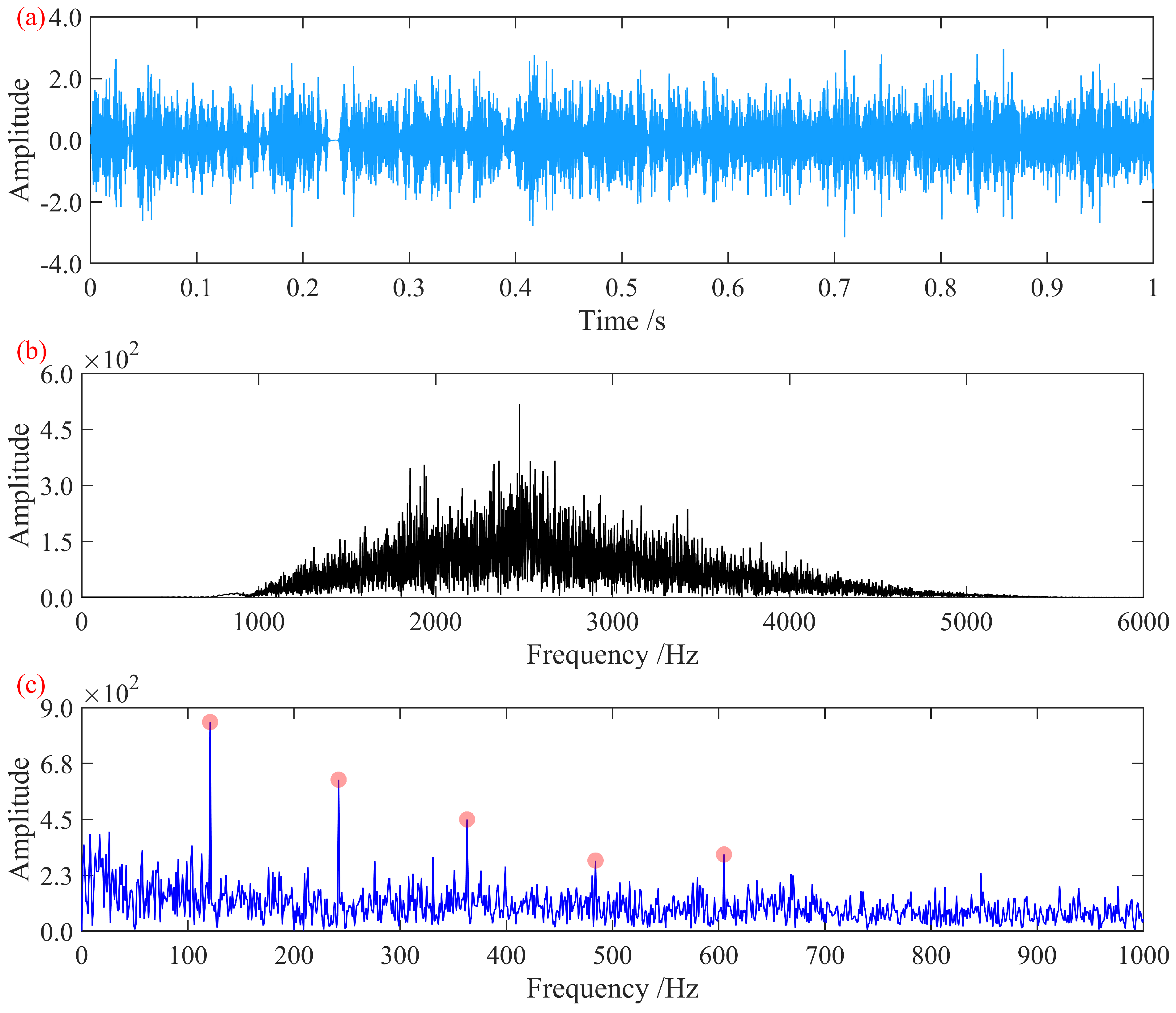
In the Hilbert envelope spectrum of the original signal, only faintly identifiable first- and second-order fault characteristic frequencies are present, with significant noise content in the spectrum masking the remaining harmonic features. To extract the hidden fault characteristics, the method proposed in this paper was employed for fault feature extraction. For the MCFECC eigenvalue, P was set to five, and r was set to 0.03. In the A-SCA, the population size was set to 10, the maximum number of iterations was set to 10, the search range for the bandwidth threshold B was set to [0.05, 0.9], and the search range for the fitting order K was set to [20, 30]. Using the negative value of the MCFECC eigenvalue as the search metric, the B and K corresponding to the minimized value were taken as the construction parameters for ISTVF-EMD to decompose the signal. Through A-SCA iteration, the optimal bandwidth threshold B for ISTVF-EMD was determined to be 0.08847, and the optimal fitting order K was determined to be 25. The optimally decomposed component signal obtained is shown in Figure 12.

Figure 12. Optimal decomposition signal: (a) time-domain waveform; (b) frequency spectrum; (c) Hilbert envelope spectrum.

The Hilbert envelope spectrum in the figure clearly shows the fault characteristic frequency at approximately 108 Hz and its first eight harmonics. This effectively reveals the outer race fault characteristic information of the bearing, enabling the extraction and diagnosis of the outer race fault from this signal.

4.2.2. Case 4

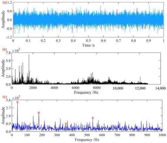
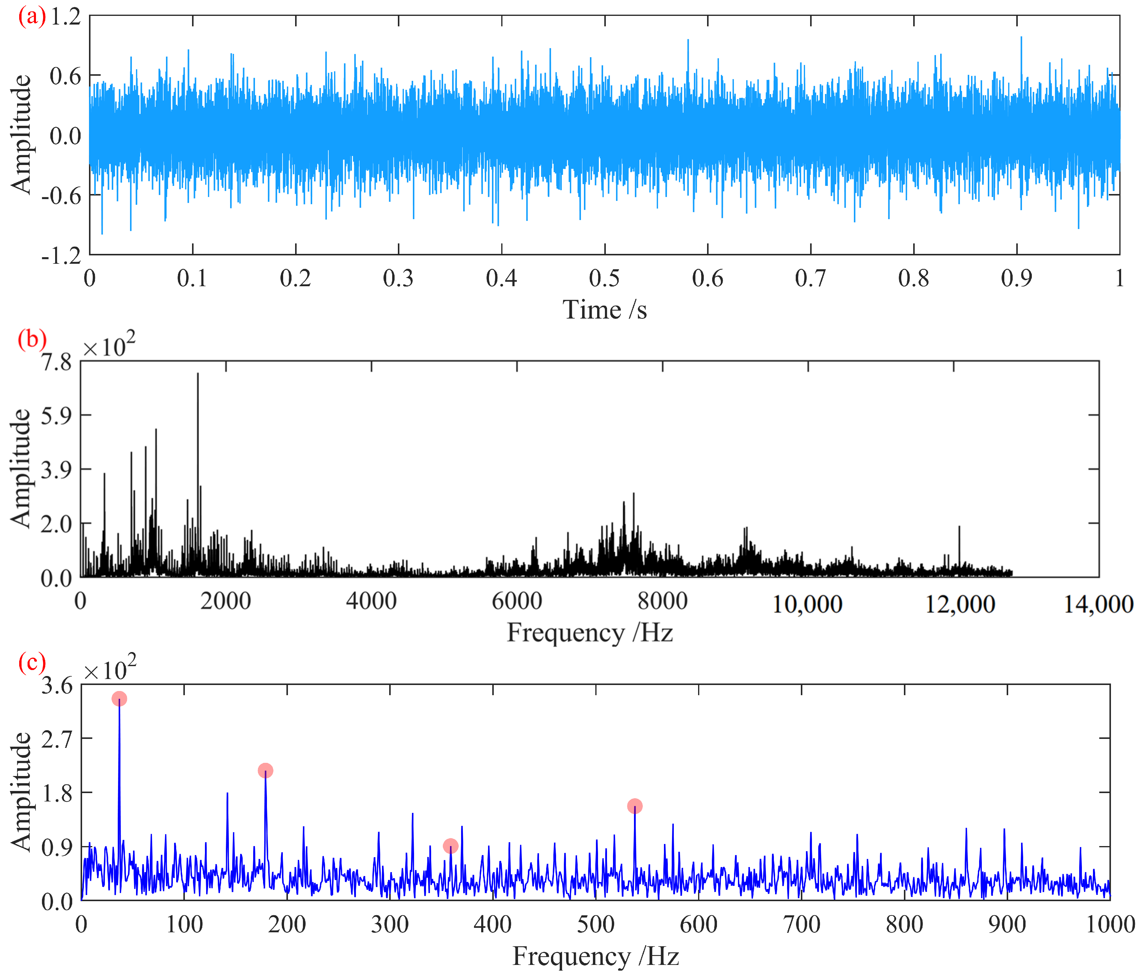
The vibration acceleration signal of the axle-box bearing with an inner race fault in Case 4 was analyzed and processed. At this rotational speed, the characteristic fault frequencies of the axle-box bearing were determined to be outer race fault frequency, 115.62 Hz; inner race fault frequency, 184.38 Hz; rolling element fault frequency, 77.5 Hz; and cage fault frequency, 14.45 Hz. The time-domain waveform and frequency spectrum of the signal, normalized to its maximum amplitude, are shown in Figure 13.

Figure 13. Signal from the bearing with an inner race fault: (a) time-domain waveform; (b) frequency spectrum; (c) Hilbert envelope spectrum.

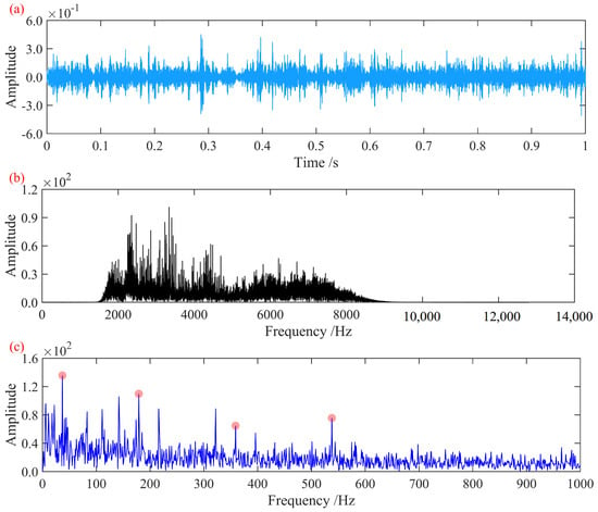
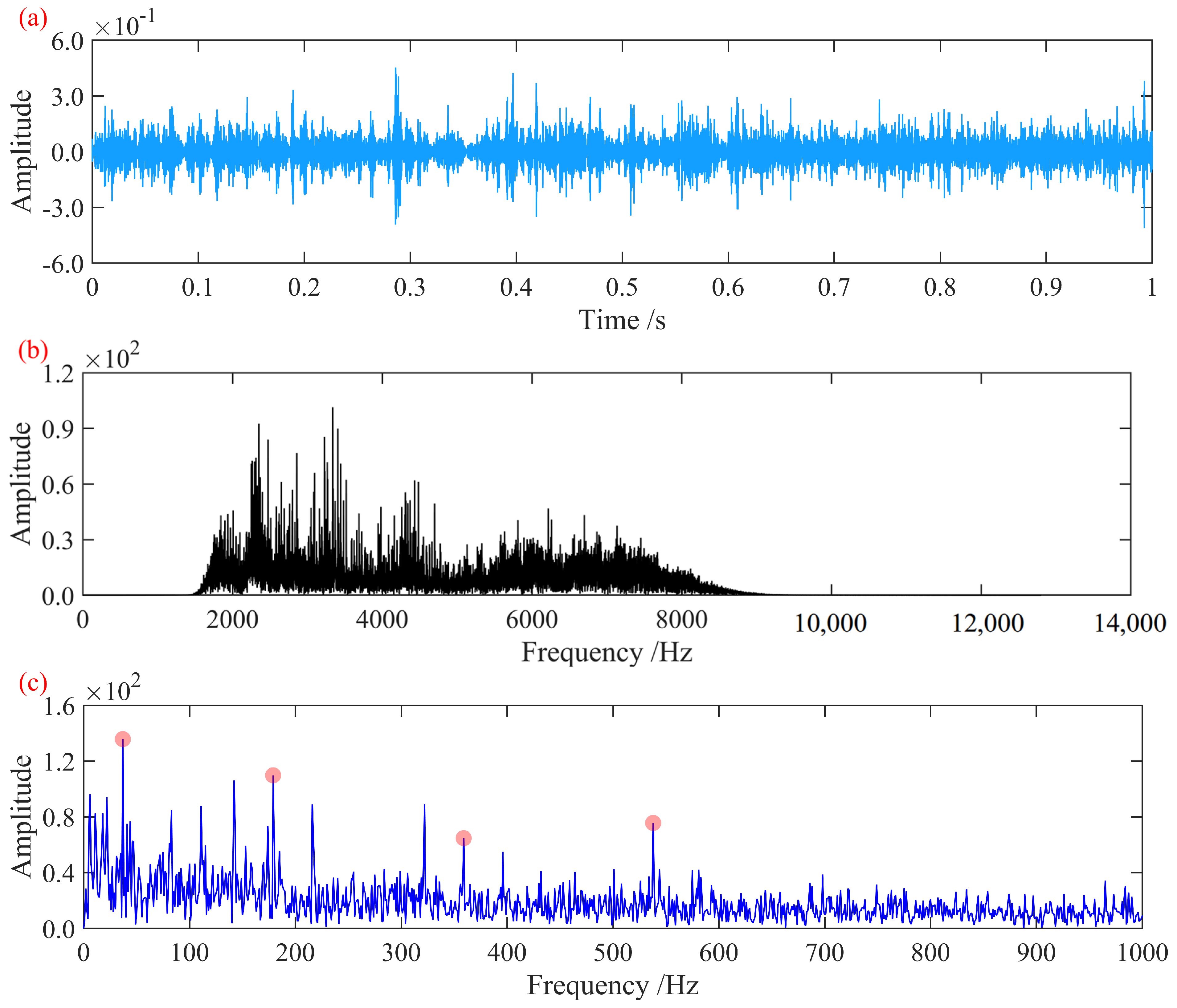
The Hilbert envelope spectrum of the original signal exhibits rotational frequency modulation components, along with relatively distinct first- and third-order inner race fault characteristic frequencies and their corresponding rotational frequency modulation sidebands. To further enhance the fault features, the proposed method was applied for fault feature extraction. The MCFECC parameters were set as P = 5 and r = 0.03. For the A-SCA, the population size was 10, the maximum number of iterations was 10, the search range for the bandwidth threshold B was [0.05, 0.9], and the search range for the fitting order K was [20, 30]. The negative value of the MCFECC feature was used as the optimization criterion to identify the optimal B and K corresponding to the minimum value. These parameters were then used to construct the ISTVF-EMD for signal decomposition. Through A-SCA iteration, the optimal bandwidth threshold B for ISTVF-EMD was determined to be 0.4502, and the optimal fitting order K was 30. The resulting optimal decomposition component signal is shown in Figure 14.

Figure 14. Optimal decomposition signal: (a) time-domain waveform; (b) frequency spectrum; (c) Hilbert envelope spectrum.

The Hilbert envelope spectrum in the figure clearly shows the fault characteristic frequency at approximately 184 Hz and its first three harmonics. Compared to the Hilbert envelope spectrum of the original signal, the spectrum here displays more pronounced modulation sidebands, and the prominence of each harmonic is significantly enhanced. The observed envelope spectrum characteristics align with the typical patterns of bearing inner race faults, demonstrating that the proposed fault diagnosis algorithm can effectively extract inner race fault characteristic information.

5. Results Analysis and Discussion

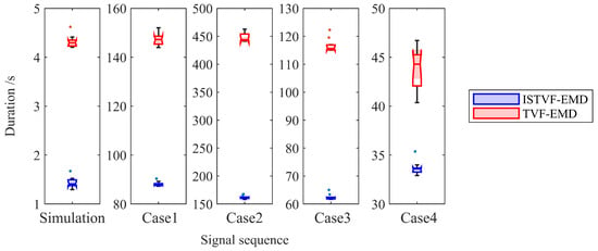
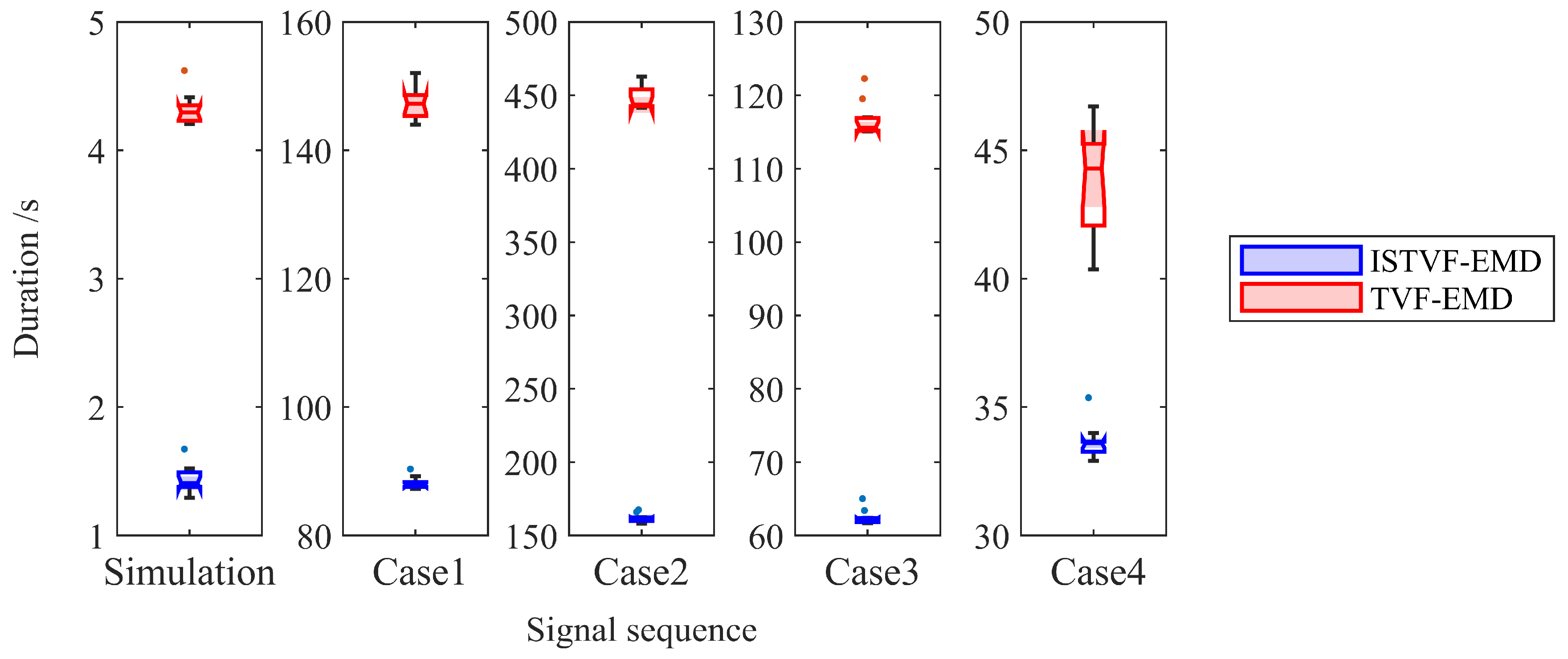
The rolling bearing fault diagnosis algorithm proposed in this paper was applied to analyze one set of simulation signals and four sets of faulty bearing test signals, all of which successfully enhanced the fault features and achieved fault diagnosis. The core of the algorithm is the ISTVF-EMD decomposition method. Compared to the original ISTVF-EMD method, the improved decomposition method proposed herein aims to increase the signal decomposition speed while maintaining decomposition effectiveness. To verify whether this intended effect was achieved, the decomposition performance of both the ISTVF-EMD and the original TVF-EMD methods was analyzed using the same decomposition parameters—specifically, the bandwidth threshold B and fitting order K obtained from the previous signal analysis for each respective signal. The statistical box plot of the execution time for 10 runs is shown in Figure 15.

Figure 15. Box plots of computational time.

The statistical results from the figure indicate that for all five sets of signals analyzed in this study, the decomposition time of ISTVF-EMD is significantly shorter than that of TVF-EMD. This acceleration effect provided by ISTVF-EMD becomes even more pronounced when swarm intelligence optimization algorithms are employed for optimal parameter searching.

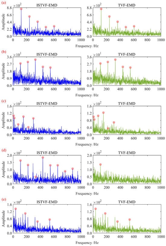
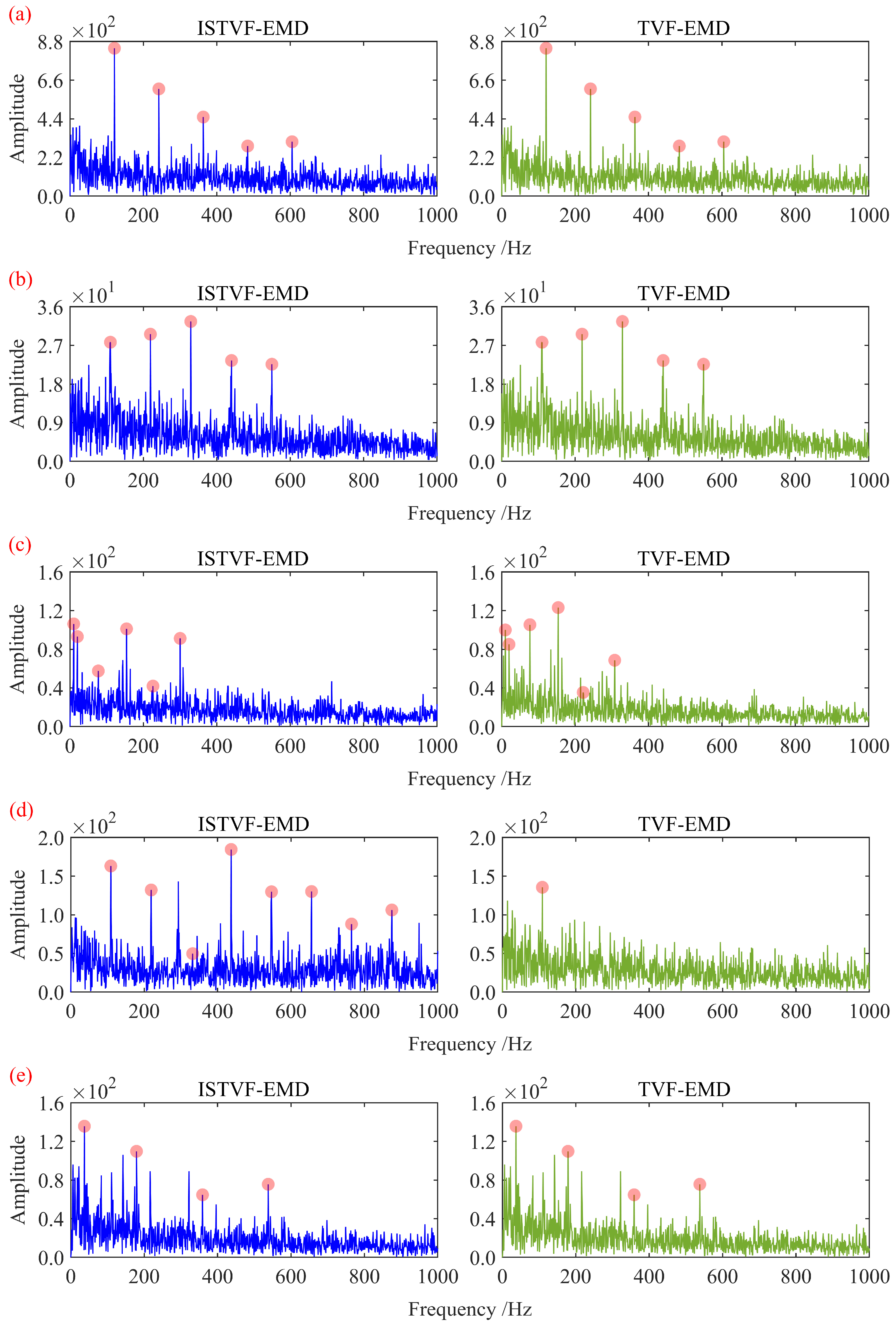
Beyond improving computational speed, ISTVF-EMD is also expected to enhance the quality of signal decomposition. Therefore, the optimal decomposition results from both ISTVF-EMD and TVF-EMD were subjected to Hilbert envelope demodulation to compare their decomposition capabilities. The corresponding Hilbert envelope spectra are shown in Figure 16.

Figure 16. Comparison of Hilbert envelope spectra for the optimally decomposed signals: (a) simulation signal; (b) experimental signal in Case 1; (c) experimental signal in Case 2; (d) experimental signal in Case 3; (e) experimental signal in Case 4.

As shown in the comparative figure, under the premise of using the same bandwidth threshold B and fitting order K, the ISTVF-EMD method not only improves the signal decomposition speed but also maintains the effectiveness of the optimal decomposed signal. For the simulation signal and the experimental signals in Cases 1 and 4, both methods yielded identical optimal decomposition results. For the experimental signals in Cases 2 and 3, the Hilbert envelope spectrum of the optimal signal decomposed by ISTVF-EMD contains a greater number of meaningful harmonic components of the fault characteristic frequencies, with Case 3 showing a particularly notable improvement. This further substantiates that ISTVF-EMD offers higher computational efficiency and superior decomposition performance.

6. Discussion

To highlight the theoretical and engineering contributions of this work, this section provides additional comparative and interpretability discussions. The focus is to clarify the differences and complementarities between the proposed ISTVF-EMD + A-SCA + MCFECC framework and previously published dimension-theory approaches, HHT/VMD-based decomposition methods, and deep learning-based techniques, in terms of mathematical formulation, physical meaning, and applicable scenarios.

6.1. Mathematical Differences and Physical Insights Compared with Dimension-Theory Methods

Dimension-theory approaches typically reveal proportional relationships and dominant mechanisms among physical quantities by nondimensionalizing governing dynamic equations, performing scale decomposition, or deriving energy/size-ratio-based analytical relations. Their outcomes primarily emphasize analytical or semi-analytical descriptions of physical laws.

In contrast, this study does not attempt to derive analytical solutions or nondimensional scaling laws directly from mechanical dynamics. Instead, it constructs a “signal–decomposition parameter–frequency energy concentration” mapping chain.

At the mathematical level, ISTVF-EMD employs a time-varying filter with finite-order B-spline approximation to achieve adaptive decomposition based on local cutoff frequency, while limiting the maximum decomposition level to avoid noise-driven over-decomposition. A-SCA performs joint global–local optimization in the two-dimensional parameter space defined by the bandwidth threshold B and fitting order K, thereby treating the parameterized decomposition operator as an optimization variable. MCFECC serves as a composite objective function that quantifies the energy concentration of physically meaningful characteristic frequency families (outer race, inner race, rolling element, and cage) in the envelope spectrum, thereby evaluating the “physical relevance” of the decomposition result.

In terms of physical interpretation, MCFECC directly quantifies the harmonic clusters and their energy concentration generated by impulsive events in the envelope spectrum, thus providing a measurable mapping from spectral patterns to fault mechanisms (intermittent impacts, modulation, coupled friction). In other words, the proposed framework links observed spectral features with underlying excitation mechanisms via signal processing and frequency-domain energy metrics, rather than only presenting nondimensional proportional relationships. Therefore, the two approaches are complementary: dimension-theory methods are more suitable for revealing fundamental mechanisms and scaling relationships, whereas the present method is more effective in extracting and amplifying signal components corresponding to physical characteristic frequencies under strong noise or experimental conditions, thereby providing clearer input features for subsequent physics-based inversion or health assessment.

6.2. Discrimination Strategy for Unbalance and Crack-Induced Interference

In practical applications, rotor unbalance, shaft cracks, backlash, and bearing defects may all produce frequency enhancement or sidebands in the spectrum. To avoid misclassifying rotor unbalance as bearing cracks or inner/outer race faults, a multi-criteria spectral decision process is adopted:

Rotor unbalance mainly manifests as stable amplitude enhancement at the fundamental frequency (1X) and its integer multiples, typically with weak higher-order harmonics and limited envelope harmonic clustering. In contrast, localized bearing defects form distinct harmonic combs at their characteristic frequencies and higher-order harmonics in the envelope spectrum.

MCFECC computes CFECC values in parallel for multiple characteristic frequency families and selects the dominant one. Thus, discrimination is based on the energy concentration at the frequency-family level. If 1X-related components dominate but no harmonic cluster associated with target bearing characteristic frequencies is observed, MCFECC does not bias toward a bearing fault diagnosis.

For possible crack-induced modulation or sidebands, the method further examines envelope spectrum sideband structures and their synchronization with rotational speed before final decision-making, thereby reducing false identification.

6.3. Functional and Performance Comparison with Deep Learning Methods (E.g., LSTM/Hybrid Models)

Deep learning approaches exhibit advantages in large-scale labeled datasets and nonlinear mapping learning, especially for end-to-end classification or regression tasks. In contrast, the proposed signal enhancement and feature extraction framework differs in the following aspects:

Unsupervised/small-sample adaptability: The ISTVF-EMD + A-SCA + MCFECC framework is a physics–frequency-driven unsupervised enhancement scheme that does not rely on large, labeled training datasets, making it suitable for data-scarce or early-stage experimental scenarios.

Strong interpretability: The outputs are physically meaningful frequencies and their harmonic clusters, enabling engineers to perform causal diagnosis. In contrast, deep models often generate black-box representations that are difficult to interpret post hoc.

Real-time/online deployment cost: Compared with GPU-dependent and training-intensive deep models, the proposed method involves relatively few parameters and can be implemented on conventional engineering computing platforms, facilitating on-site quasi-real-time monitoring.

6.4. Advantages and Limitations Compared with HHT/Conventional EMD/VMD

HHT and classical EMD have made significant contributions to non-stationary signal decomposition, but often suffer from mode mixing and noise-driven over-decomposition under low SNR conditions. VMD and its variants improve stability by enforcing fixed bandwidth and predefined mode numbers, but parameter selection remains challenging.

In comparison, ISTVF-EMD controls decomposition granularity through time-varying filtering and bandwidth thresholds, while introducing a maximum decomposition level constraint to prevent the generation of excessive narrow-band IMFs under low SNR conditions, thus improving computational efficiency and stability.

A-SCA incorporates the key decomposition parameters B and K into a global optimization framework driven by the MCFECC metric, thereby reducing manual parameter tuning.

In multiple simulations and experiments, ISTVF-EMD significantly reduces computational time while maintaining or improving decomposition quality (see Figure 15).

In terms of limitations, when severe frequency overlap or strongly coupled dynamics are present, purely spectrum-concentration-based evaluation may be insufficient to fully isolate all causal factors. In such cases, integration with physics-based modeling or multi-sensor fusion is recommended.

6.5. Innovation and Physical Significance of MCFECC

MCFECC computes multiple envelope-spectrum-based energy concentration indices in parallel and performs selection at the characteristic frequency family level, providing three key advantages:

No prior fault-type requirement: Unlike metrics requiring predefined fault types, MCFECC enables blind dominant-frequency discovery by evaluating all common bearing characteristic frequencies in parallel.

Frequency-family competition mechanism: By comparing the energy concentration of different characteristic frequency families, the method automatically identifies the most physically relevant spectral structure in the current signal.

Enhanced physical traceability: When MCFECC indicates a specific characteristic frequency family, the observed harmonic clusters and sideband structures can be directly mapped back to corresponding mechanical excitation or contact forms.

6.6. Applicability and Limitations Under Variable Load, Variable Speed, and Multi-Rotor Systems

Several design features support applicability under industrial conditions. MCFECC calculates characteristic frequencies based on real-time rotational speed, and A-SCA performs independent optimization for each signal segment, providing robustness against abrupt operating-condition variations.

For multi-rotor or coupled systems, the framework can be directly extended by incorporating theoretical characteristic frequencies of all rotors and bearings into the MCFECC calculation. However, under strong coupling or highly overlapping spectral conditions, the resolution of a single-channel envelope spectrum may be limited. In such cases, multi-channel signal fusion, spatial filtering, or dynamic-model-based decoupling preprocessing may be required.

6.7. Verification of Early Fault Detection Under Low SNR Conditions

To demonstrate detection capability under early-fault conditions, simulations and several experimental signals show that, through bandwidth and decomposition-level constraints in ISTVF-EMD and adaptive parameter optimization via A-SCA, harmonic clusters in the envelope spectrum can be enhanced and multi-order harmonic information can be restored (see Figure 5 and Figure 8, and 12). These results indicate high detection sensitivity under weak impulsive environments.

7. Conclusions

In this study, an adaptive bearing fault diagnosis framework integrating ISTVF-EMD, A-SCA parameter optimization, and the MCFECC energy concentration index was proposed. The method was validated through both simulation analysis and experimental datasets, demonstrating improved decomposition stability and enhanced weak-fault feature extraction capability.

(1)

Simulation results under low signal-to-noise ratio conditions verified the robustness of the proposed method. At −13 dB SNR, the harmonic comb structure of the theoretical characteristic frequency was still clearly preserved. Compared with classical EMD, the number of effective intrinsic mode functions (IMFs) was reduced from 11 to six, indicating a more compact and physically meaningful decomposition. Meanwhile, the average computation time per signal segment decreased from 2.31 s to 1.42 s, confirming improved computational efficiency.

(2)

The introduction of the MCFECC index further enhanced the concentration of characteristic frequency energy. Experimental results showed that harmonic components up to the sixth order could be clearly identified in the envelope spectrum, and the energy aggregation around the fault characteristic frequency was significantly strengthened compared with conventional decomposition strategies.

(3)

Validation on the Southwest Jiaotong University axle-box bearing test rig and Xi’an Jiaotong University bearing test rig further confirmed the practical applicability of the proposed framework. Under a rotational speed of 500 r/min and a radial load of 0.5 t, the extracted dominant fault frequency (61.6 Hz) closely matched the theoretical value (61.5 Hz), with a relative error below 0.5%, demonstrating high frequency localization accuracy and strong physical consistency.

(4)

Overall, the proposed method achieves stable adaptive decomposition, enhanced weak-feature detectability under low-SNR conditions, and accurate characteristic frequency localization, while maintaining acceptable computational cost. These results indicate that the framework provides both theoretical interpretability and practical applicability for rolling bearing fault diagnosis.

Future work will focus on extending the method to more complex operating conditions and multi-sensor fusion scenarios to further improve robustness in real industrial environments.

References

- Li, J.; Luo, W.; Bai, M. Review of research on signal decomposition and fault diagnosis of rolling bearing based on vibration signal. Meas. Sci. Technol. 2024, 35, 092001. [Google Scholar] [CrossRef] [Scilit]
- Zheng, Z.; Song, D.; Zhang, W.; Chen, R.; Ma, C.; Cui, W.; Xu, X. An optimal filtering frequency band search method based on MZGWO in rolling bearings fault diagnosis. Mech. Syst. Signal Process. 2025, 232, 112773. [Google Scholar] [CrossRef] [Scilit]
- Li, W.; Chen, J.; Li, J.; Xia, K. Derivative and enhanced discrete analytic wavelet algorithm for rolling bearing fault diagnosis. Microprocess. Microsyst. 2021, 82, 103872. [Google Scholar] [CrossRef] [Scilit]
- Ma, Z.; Zhang, Y. A study on rolling bearing fault diagnosis using RIME-VMD. Sci. Rep. 2025, 15, 4712. [Google Scholar] [CrossRef] [Scilit]
- Hu, Y.; Zhao, E.; Li, J.; Li, J.; Zhao, X.; Ma, B.; Dong, M. Fault diagnosis of rolling bearing based on SEMD and ISSA-KELMC. Meas. Sci. Technol. 2024, 35, 056127. [Google Scholar] [CrossRef] [Scilit]
- Liu, X.; Yan, C.; Lv, M.; Li, S.; Wu, L. Multi-rolling element faults diagnosis of rolling bearing based on time-frequency analysis and multi-curves extraction. Meas. Sci. Technol. 2024, 35, 106113. [Google Scholar] [CrossRef] [Scilit]
- Wang, Z.; Yang, J.; Guo, Y. Unknown fault feature extraction of rolling bearings under variable speed conditions based on statistical complexity measures. Mech. Syst. Signal Process. 2022, 172, 108964. [Google Scholar] [CrossRef] [Scilit]
- Guo, Y.; Yang, Y.; Jiang, S.; Jin, X.; Wei, Y. Rolling bearing fault diagnosis based on successive variational mode decomposition and the EP index. Sensors 2022, 22, 3889. [Google Scholar] [CrossRef] [Scilit]
- Sun, W.; Sun, Y.; Wang, Y. Integrated fault diagnosis of rolling bearings based on improved multichannel singular spectrum analysis and frequency-spatial domain decomposition. Meas. Sci. Technol. 2023, 34, 035116. [Google Scholar] [CrossRef] [Scilit]
- Li, X.; Sun, J. A novel method for diagnosing rolling bearing faults based on the frequency spectrum distribution of the modulation signal. Meas. Sci. Technol. 2022, 33, 085003. [Google Scholar] [CrossRef] [Scilit]
- Ma, J.; Li, H.; Tang, B.; Wang, J.; Zou, Z.; Zhang, M. Rolling bearing fault diagnosis based on improved VMD-adaptive wavelet threshold joint noise reduction. Adv. Mech. Eng. 2022, 14, 16878132221128397. [Google Scholar] [CrossRef] [Scilit]
- Liu, M.; Shen, Y.; Xu, Y. A resonance-identification-guided autogram for the fault diagnosis of rolling element bearings. Machines 2025, 13, 169. [Google Scholar] [CrossRef] [Scilit]
- Tian, S.; Zhen, D.; Li, H.; Feng, G.; Zhang, H.; Gu, F. Adaptive resonance demodulation semantic-induced zero-shot compound fault diagnosis for railway bearings. Measurement 2024, 235, 235. [Google Scholar] [CrossRef] [Scilit]
- Wu, Z.; Chen, W.; Zhang, X.; Liu, F.; Zhang, X.; Guo, Q. An optimal demodulation frequency band selection method based on spectral coherence fault energy factor for rolling bearing fault diagnosis. Proc. Inst. Mech. Eng. Part C J. Mech. Eng. Sci. 2025, 239, 598–612. [Google Scholar] [CrossRef] [Scilit]
- Luan, X.; Zhong, C.; Zhao, F.; Sha, Y.; Liu, G. Bearing fault damage degree identification method based on SSA-VMD and Shannon entropy-exponential entropy decision. Struct. Health Monit. 2024, 23, 3102–3133. [Google Scholar] [CrossRef] [Scilit]
- Li, S.; Zhao, M.; Wei, Y.; Ou, S.; Chen, D.; Wu, L. Adaptive residual spectral amplitude modulation: A new approach for bearing diagnosis under complex interference environments. Mech. Syst. Signal Process. 2024, 220, 111682. [Google Scholar] [CrossRef] [Scilit]
- Chen, T.; Guo, L.; Gao, H.; Feng, T.; Yu, Y. Clustering Weighted Envelope Spectrum for Rolling Bearing Fault Diagnosis. IEEE Trans. Autom. Sci. Eng. 2025, 22, 3922–3932. [Google Scholar] [CrossRef] [Scilit]
- Shang, J.; Dai, J.; Hu, Y.; Hu, D.; Zeng, X.; Yu, T. Fault diagnosis method of traction motor bearings based on optimized weight local kurtosis. Transp. Saf. Environ. 2025, 7, tdaf018. [Google Scholar] [CrossRef] [Scilit]
- Li, H.; Li, Z.; Mo, W. A time varying filter approach for empirical mode decomposition. Signal Process. 2017, 138, 146–158. [Google Scholar] [CrossRef] [Scilit]
- E, X.; Wang, W.; Yuan, H. Bearing fault feature extraction method based on adaptive time-varying filtering empirical mode decomposition and singular value decomposition denoising. Machines 2025, 13, 50. [Google Scholar] [CrossRef] [Scilit]
- Mirjalili, S. SCA: A sine cosine algorithm for solving optimization problems. Knowl.-Based Syst. 2016, 96, 120–133. [Google Scholar] [CrossRef] [Scilit]
- Ma, W.; Liu, R.; Guo, J.; Wang, Z.; Ma, L. A collaborative central domain adaptation approach with multi-order graph embedding for bearing fault diagnosis under few-shot samples. Appl. Soft Comput. 2023, 140, 110243. [Google Scholar] [CrossRef] [Scilit]
- Chen, B.; Song, D.; Zhang, W.; Cheng, Y.; Wang, Z. A performance enhanced time-varying morphological filtering method for bearing fault diagnosis. Measurement 2021, 176, 109163. [Google Scholar] [CrossRef] [Scilit]
- Li, Q.; Chen, B.; Zhang, W.; Song, D. Research on mathematical morphological operators for fault diagnosis of rolling element bearings. Measurement 2022, 203, 111964. [Google Scholar] [CrossRef] [Scilit]
- Wang, Z.; Zheng, Z.; Song, D.; Xu, X. A high-speed train axle box bearing fault diagnosis method based on dimension reduction fusion and the optimal bandpass filtering demodulation spectrum of multi-dimensional signals. Machines 2024, 12, 571. [Google Scholar] [CrossRef] [Scilit]
- Sawalhi, N.; Randall, R. Simulating gear and bearing interactions in the presence of faults: Part I: The combined gear bearing dynamic model and the simulation of localised bearing faults. Mech. Syst. Signal Process. 2008, 22, 1924–1951. [Google Scholar] [CrossRef] [Scilit]
- Wang, B.; Lei, Y.; Li, N.; Li, N. A hybrid prognostics approach for estimating remaining useful life of rolling element bearings. IEEE Trans. Reliab. 2020, 69, 401–412. [Google Scholar] [CrossRef] [Scilit]
Disclaimer/Publisher’s Note: The statements, opinions and data contained in all publications are solely those of the individual author(s) and contributor(s) and not of MDPI and/or the editor(s). MDPI and/or the editor(s) disclaim responsibility for any injury to people or property resulting from any ideas, methods, instructions or products referred to in the content. |
© 2026 by the authors. Licensee MDPI, Basel, Switzerland. This article is an open access article distributed under the terms and conditions of the Creative Commons Attribution (CC BY) license.