Artificial Bee Colony Algorithm-Based Optimization for Reducing Tooth Flank Distortion in Form-Grinding

Abstract

The tooth flank distortion error occurring during the form-grinding (FG) of an involute helical gear can significantly compromise transmission performance. Conventional research approaches often focus on single-parameter optimization—either the grinding wheel installation angle (GWIA) or the contact line (CL)—without adequately accounting for the coupling relationships among GWIA, CL, and the modification curve (MC). To address this limitation, this study proposes an innovative joint optimization approach that simultaneously optimizes GWIA, CL, and MC to effectively minimize tooth flank distortion in FG. Based on the principles of form-grinding, a mathematical model is established for the contact line of the target gear and the cross-sectional profile of the grinding wheel. The relationship between GWIA and tooth flank deviation is investigated using a proprietary virtual prototype. A multi-objective artificial bee colony (ABC) optimization algorithm is employed to determine the optimal values of GWIA and CL. For the axial modification curve, this paper introduces a novel three-segment quadratic curve optimization scheme as an improvement over conventional modification methods. To validate the proposed optimization technique, form-grinding experiments are conducted on the L300G gear grinding machine. Simulation outcomes indicate that, pre-optimization, the maximum tooth flank distortion errors primarily occur at the tooth root and tip regions on both ends of the gear. After optimization, the simulated distortion error on the left tooth flank is reduced by 48.5%, while the right flank shows a reduction of 29.4%. These simulation outcomes exhibit a deviation of approximately 10% compared with the experimental results. This study provides valuable insights for enhancing the transmission performance of helical gears.

1. Introduction

Under real operating conditions, manufacturing inaccuracies, assembly misalignment, and bearing deformation induce eccentric loading and stress concentration in gear transmission systems. Axial modification of helical gears can mitigate these issues; however, the modification grinding process requires additional grinding wheel motion. Due to the helix angle, an inherent distortion error arises: one end of the gear exhibits over-correction at the tooth tip and under-correction at the root, while the opposite occurs at the other end. This results in tooth flank distortion, significantly degrading transmission performance.

Significant research efforts have been devoted to reducing distortion effects in helical gear form-grinding and axial modification, both domestically and internationally. He et al. [1] proposed an error compensation method for multi-axis additional motion optimization to address the problem of tooth flank distortion in helical gear axial modification, reducing the tooth flank distortion error by 93%. Taking the herringbone gear as the research object, Jiang et al. [2] proposed a modified tooth flank optimization design method with small wheel floating installation. Zhang et al. [3] took polynomial coefficients as variables and the minimum tooth flank error of topological modification as the optimization objective to solve the optimal polynomial coefficients of each moving axis of the machine tool. He et al. [4] proposed a joint optimization method for the grinding wheel installation angle and the grinding wheel cross-section in order to improve the axial modification accuracy of helical gears. The accuracy of this method was verified by experiments. Guo et al. [5] optimized the contact line between the grinding wheel and workpiece installation parameters to reduce distortion errors and improve gear transmission performance. Wang et al. [6] implemented topological modifications to gears to reduce noise during meshing. Li et al. [7] put forward an optimization method for grinding wheel cross-sections to reduce grinding error. The least square method was used to settle the fitting points of the GW at different times, and these point clouds were connected into the optimized grinding wheel profile. Su et al. [8] proposed an optimized design for linear diagonal modification of form-grinding herringbone gear in order to reduce vibration and noise under actual working conditions. Li et al. [9] optimized the GWIA by using the PSO algorithm to reduce the tooth flank distortion and improve the machining accuracy. Li et al. [10] optimized the GWIA to weaken the tooth flank distortion problem of helical gear axial modification. The above studies mostly focus on optimizing the GWIA, the CL, and the cross-section of the grinding wheel for the tooth flank distortion in the form-grinding. However, there are few studies on optimizing the axial modification curve.

By employing a multi-objective genetic algorithm (GA), Wang [11] investigated the simultaneous optimization of the RMS value and the static weight distribution uniformity over the tooth flank to derive the optimal modification parameters. Yao [12] took the MATLAB optimization toolbox as the method to conduct multi-objective optimization of volume and overlap degree to boost the stability of gear transmission. Younes et al. [13] employed the NSGA-II algorithm to optimize both microscopic and macroscopic geometric parameters, aiming to minimize power loss and reduce vibration in gear transmission systems. To enhance the performance of helical gear transmission systems, He et al. [14] employed the NSGA-II algorithm to solve a functional model established on a Back-Propagation neural network. Zhou et al. [15] applied the NSGA-II algorithm to identify optimal helical gear meshing parameters, aiming to increase the load capacity of the transmission system while mitigating vibration and noise. Han et al. [16] used a multi-objective GA to optimize machine tool motion trajectories for improved tooth flank modification accuracy. By investigating the sensitivity of polynomial coefficients to normal deviations in gear tooth topography, Shih et al. [17] established that their optimization leads to a tooth form that more closely approximates the theoretical flank. To address the reduction of vibrational excitation forces, Yuan et al. [18] formulated a multi-objective optimization framework for tooth flank modification. Their approach coupled an LTCA model with the NSGA-II algorithm, thereby deriving the Pareto-optimal parameter set. Through an investigation of how tip relief affects spur gear meshing vibrations, Rogkas N et al. [19] employed KISSsoft software, with gear efficiency, service life, and geometric volume designated as the design variables, and the objectives set to maximize transmission efficiency and torque capacity, while simultaneously minimizing wear rate and noise emission.

The above studies mostly use the NSGA-II algorithm for multi-objective optimization, while at present, there are few studies using the ABC algorithm for multi-objective optimization. Compared with GA, the ABC algorithm has stronger global search ability, fewer parameters, straightforward implementation, and strong robustness. Lin TJ et al. [20] took into account the manufacturing and installation errors of the gear system, analyzed the gear transmission errors before and after modification, and established a dynamic model of the transmission system based on the concentrated mass method to solve the dynamic transmission errors of the gear transmission system. Tian XQ et al. [21] aimed to solve the problem of distortion of the tooth flank after axial modification, and proposed a contact line evaluation genetic algorithm. This method is achieved by adjusting the motion axis and does not require any grinding of the grinding wheel. Yan PF et al. [22] considered the meshing errors caused by factors such as gear manufacturing errors and installation deviations, and constructed a distributed lateral-torsional-sway coupling nonlinear dynamic model of the helical gear pair; subsequently, they proposed an optimization method based on the regulation of the tooth width parameter to improve the uniformity of the tooth surface load distribution. Liu YP et al. [23] adopted the method of axial modification to improve the contact stress. They studied the influence laws of different axial modification amounts and lengths on the contact stress of the tooth surface, the stress at the tooth root, and the transmission error. Gao P et al. [24] The tooth profile parameters are designated as independent variables, while the system’s dynamic load coefficient serves as the optimization objective. Boundary conditions are established based on the driving wheel’s rotational speed and the applied load torque.

This paper presents an innovative joint optimization method integrating GWIA, CL, and axial MC to minimize tooth flank distortion in form-grinding axial modification processes. Based on form-grinding principles, we first establish mathematical models for both the CL and grinding wheel profile of the target gear. A multi-objective ABC optimization algorithm is then developed to simultaneously determine the optimal grinding wheel installation angle and spatial contact line morphology. For the modification curve, we introduce an innovative approach using a composite three-segment quadratic curve design to replace conventional modification profiles. Experimental validation conducted on our self-developed L300G CNC gear grinding machine confirms the effectiveness in improving axial modification accuracy and distortion reduction.

2. Form-Grinding Processing Test Platform

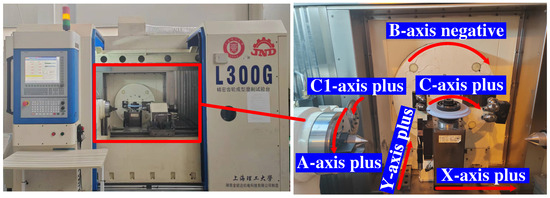
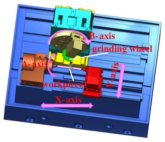
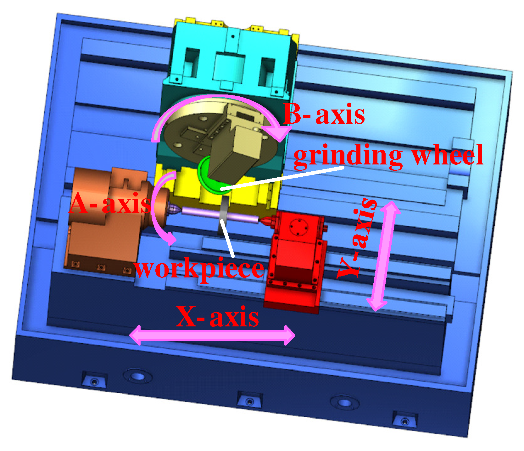
The experimental work is carried out on an L300G gear grinding machine (Figure 1), which is independently developed by our research group. The machine configuration includes two linear axes (X, Y) and four rotary axes dedicated to workpiece (A), grinding wheel (B), dressing wheel (C1), and tool spindle (C) movements.

Figure 1. Structural schematic of the L300G gear grinding machine.

The forming method for gear grinding mainly consists of two steps: Firstly, the dressing wheel performs the truing and dressing of the grinding wheel according to its coordinate points; Secondly, grinding gear blanks with trimmed grinding wheels. While the grinding of standard helical gear is accomplished through the linkage of the X, A, and C axes, the process for axial modification necessitates additional grinding wheel motion, engaging the A, X, C, and Y axes in a coordinated manner. The machine tool, installed on shock absorption devices, operated within a thermostatic chamber held at 20 °C.

3. A Modeling Approach for the Grinding Wheel Profile in Form-Grinding

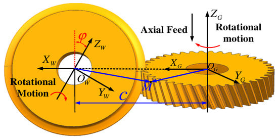
As illustrated in Figure 2, two coordinate systems are defined. The tool coordinate system is established with its origin at the grinding wheel center, the $Z_W$ along the wheel axis, and the $X_W$ along its radial direction. Similarly, the workpiece coordinate system has its origin at the gear center, with the $Z_G$ along the gear axis and the $X_G$ along the gear’s radial direction; note that the $X_W$ and $X_G$ axes are collinear. The grinding wheel is installed at an angle ($\phi$), with a center distance (C) separating the origins of the two coordinate systems. During the grinding process, the tool and workpiece intersect at a transient point M, which can be represented in both the workpiece ($O_G-X_G{Y}_G{Z}_G$) and tool ($O_W-X_W{Y}_W{Z}_W$) coordinate systems.

$$\left\{\begin{array}{c}\overrightarrow{W_M}=X_{WM}\overrightarrow{r}+Y_{WM}\overrightarrow{s}+Z_{WM}\overrightarrow{t}\\ \overrightarrow{G_M}=X_{GM}\overrightarrow{r^{\prime }}+Y_{GM}\overrightarrow{s^{\prime }}+Z_{GM}\overrightarrow{t^{\prime }}\end{array}\right.$$

(1)

Figure 2. Kinematic relationship between the gear and the grinding wheel.

In Equation (1), $X_{WM}$, $Y_{WM}$, $Z_{WM}$ and $X_{GM}$, $Y_{GM}$, $Z_{GM}$ respectively represent the projections of the vector on each coordinate axis, while $\overrightarrow{r}$, $\overrightarrow{s}$, $\overrightarrow{t}$ and $\overrightarrow{r^{\prime }}$, $\overrightarrow{s^{\prime }}$, $\overrightarrow{t^{\prime }}$ respectively represent the unit vectors on each axis of the two coordinate systems. The spatial relationship between the grinding wheel and workpiece coordinate systems can be mathematically represented by the following transformation

$$\left\{\begin{array}{l}{X}_W=X_G-C\hfill \\ Y_W=Y_G\cos \phi +Z_G\sin \phi \hfill \\ Z_W=-Y_G\sin \phi +Z_G\cos \phi \hfill \end{array}\right.$$

(2)

Given the grinding wheel angular velocity (${\omega }_M$), gear angular velocity (${\omega }_G$), and helix parameter ($P$), the relative motion velocity at point M can be derived as:

$$\overrightarrow{V_{GW}}=\overrightarrow{V_G}-\overrightarrow{V_W}={\omega }_G\left(\overrightarrow{k^{\prime }}\times \overrightarrow{G_M}+P\overrightarrow{k^{\prime }}\right)-{\omega }_W\left(\overrightarrow{k}\times \overrightarrow{W_M}\right)$$

(3)

The continuous tangential contact between the grinding wheel and the gear requires that, at the contact point, the common normal is perpendicular to the relative velocity direction between the flanks, satisfying:

$$\overrightarrow{V_{GW}}\cdot \overrightarrow{n}=0$$

(4)

${\omega }_G=\left(0,0,1\right)$, ${\omega }_W=\left(0,-\sin \phi ,\cos \phi \right)$. The contact line equation can be derived by substituting Equation (1) into Equation (4) [25]:

$$(C-X_{WM}+Pcot\phi )n_z+c{n}_{y}cot\phi +Z_{WM}{n}_x=0$$

(5)

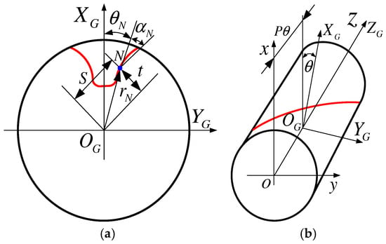
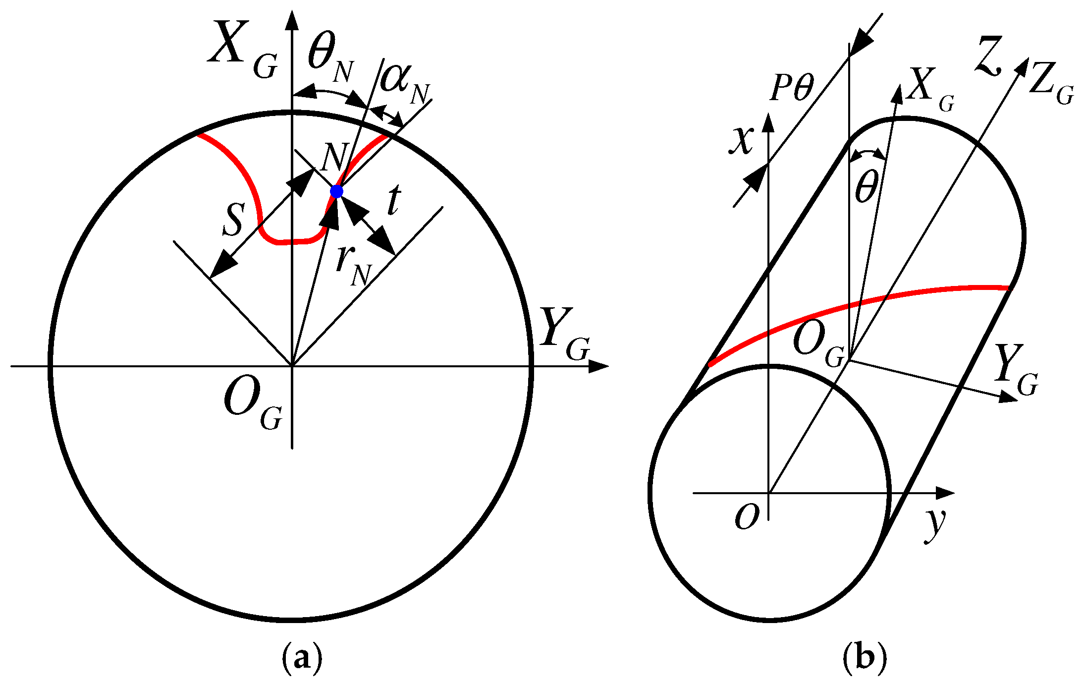
In Equation (5), $n_x$, $n_y$ and $n_z$ are the components of the normal vector at the contact point. This normal vector is used to determine the grinding wheel’s cross-section from the profile of the gear end-face tooth groove (Figure 3). The position vector of any point on this tooth groove profile is formulated in polar coordinates.

Figure 3. Schematic diagram of end face tooth groove: (a) The profile of the polar coordinate end face tooth groove; (b) Schematic diagram of the helical line.

The tooth groove cross-section of the gear end face can be expressed in polar coordinates as:

$$\left\{\begin{array}{c}{X}_G=r_{N}cos{\theta }_N\\ Y_G=r_{N}sin{\theta }_N\\ Z_G=0\end{array}\right.$$

(6)

The parameters in Equation (6) are defined for any point on the end-face tooth groove section: the position vector ($r_N$), the polar angle (${\theta }_N$), and the local tangent inclination angle (${\alpha }_N$).

The mathematical representation of the helical flank of the gear can be formulated as

$$\left\{\begin{array}{c}{X}_G=r_{N}cos({\theta }_N+\theta )\\ Y_G=r_{N}sin({\theta }_N+\theta )\\ Z_G=P\theta \end{array}\right.$$

(7)

The normal vector at any point on the helical flank is given by:

$$\left\{\begin{array}{l}{n}_x=P{\displaystyle \frac{sin\tau }{cos{\alpha }_N}}\\ n_y=-P{\displaystyle \frac{cos\tau }{cos{\alpha }_N}}\\ n_z=r_N\end{array}\right.$$

(8)

In Equation (8), $\tau$ denotes the inclination angle of the tangent line at point M on the cross-sectional profile. With a given polar angle ${\theta }_N$, the corresponding values of the position vector $r_N$ and the tangent angle ${\alpha }_N$ are subsequently obtained.

$${\alpha }_N=arctan\left(r_N/{\displaystyle \frac{d{r}_N}{d{\theta }_N}}\right)$$

(9)

Substituting Equations (7) and (8) into Equation (5) yields:

$$\begin{array}{l}(C-r_{N}cos(\tau -{\alpha }_N)+Pcot\phi )r_N-{\displaystyle \frac{CPcos\tau cot\phi }{cos{\alpha }_N}}+\\ P^2(\tau -{\theta }_N-{\alpha }_N){\displaystyle \frac{sin\tau }{cos{\alpha }_N}}=0\end{array}$$

(10)

Equation (8) can be transformed into:

$$\left\{\begin{array}{l}{n}_x={\displaystyle \frac{(C+Pcot\phi )r_{N}cos{\alpha }_N}{P^2}}\\ n_y={\displaystyle \frac{CPcot\phi +{(r_{N}cos{\alpha }_N)}^2}{P^2}}\\ n_z={\displaystyle \frac{-r_N^{2}cos{\alpha }_{K}sin{\alpha }_K}{P^2}}-{\theta }_N-{\alpha }_N\end{array}\right.$$

(11)

Substituting Equation (11) into Equation (10) yields:

$${\displaystyle \frac{n_{y}cos\tau -n_x}{sin\tau }}-\tau -n_z=0$$

(12)

Equation (12) is a transcendental equation concerning $\tau$. By using the Newton iterative method [25] to solve this equation, the coordinates of each point on the spatial contact line can be obtained. The contact line coordinates are converted from the gear system to the grinding wheel system via the coordinate transformation of Equation (2). This set of points is then subjected to a rotation about the grinding wheel axis and a subsequent projection to obtain the final cross-sectional profile of the grinding wheel.

4. Methodology for the Design and Modeling of Axial Modification

4.1. Axial Modification Design

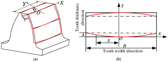
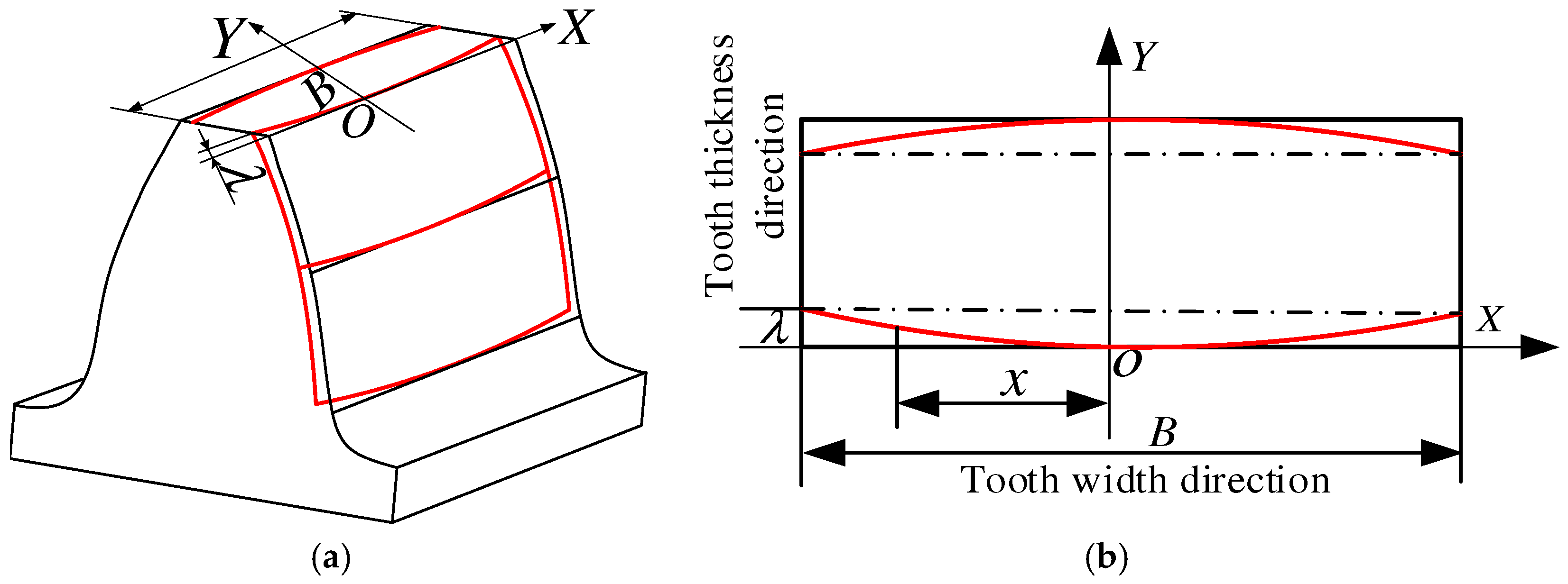
The axial modification of the forming method requires additional movement of the grinding wheel to be achieved. Traditional axial modification techniques are classified into two types: single-sided and double-sided modification. The single-sided method, accomplished by modifying either the gear’s rotational angle or the wheel’s axial movement, effectively prevents tooth flank distortion. While this advantage is significant, it suffers from comparatively low processing efficiency. As a consequence, this paper adopts the double-sided modification method. The grinding wheel needs additional center distance variation to realize. The current modification methods are divided into tooth end straight line, tooth end arc and drum-shaped modification. This study employs a drum-shaped modification strategy, the schematic representation of which is provided in Figure 4.

Figure 4. Design of the drum modification curve: (a) Front view of the drum profile; (b) Top view of the drum profile.

Figure 4 shows the coordinate system for axial modification, with its origin at the tooth width midpoint. In this system, $B$ is the total tooth width and $\lambda$ is the maximum modification amount. The modification profile is symmetric about the Y-axis, with zero modification at the center. The modification value at a distance from the center is described by the following expression:

$$y(x)={\displaystyle \frac{4\lambda }{B^2}}{x}^2$$

(13)

The axial modification value at any given section along the tooth width must be transformed into an additional motion of the GW, as described by the following expression:

$$\mathsf{\Delta }Y(x)={\displaystyle \frac{y(x)cos{\beta }_b}{sin{\alpha }_n}}$$

(14)

In Equation (14), $\mathsf{\Delta }Y(x)$ represents the variation in the center distance of the grinding wheel with any cross-section, ${\beta }_b$ represents the helix angle of the base circle, ${\alpha }_n$ represents the normal pressure angle, and $y(x)$ represents the axial modification amount of any cross-section in the tooth width direction.

4.2. Mathematical Model of Arbitrary Vector Diameter Axial Modification Amount

The modification amount along the tooth width is solved using the relative method. Accordingly, the axial modification curve (Figure 5) is designed with zero modification at the tooth center. The probe contact at this center gives a reference rotation angle ${\theta }_M$, while angles at other measurement points are ${\theta }_i$ ($i=1,2,3 ...,N$). Helical gear measurement requires linkage of the A-axis through a specified angle $\Delta A$.

$$\Delta A={\displaystyle \frac{360\times \Delta L\times sin\beta }{\pi \times M_n\times Z}}$$

(15)

$$\Delta L={\displaystyle \frac{\Delta x}{N-1}}$$

(16)

Figure 5. Model of gear grinding simulation machine tool.

In Equations (15) and (16), $\beta$ denotes the helix angle, $N$ refers to the number of measuring points, $\Delta x$ signifies the effective face width, and $\Delta L$ represents the interval length.

The practical rotation angle of the gear at each measurement point can be expressed as:

$${\theta }_{Si}={\theta }_i+(i-1)\Delta A$$

(17)

At each measuring point, the deviation of the actual gear rotation angle from its value at the tooth width center is given by:

$${\theta }_{Mi}={\theta }_{Si}-{\theta }_M$$

(18)

Let the radius of the vector diameter at any position along the tooth height be $X_K$, then the modification amount at the vector diameter at any position can be expressed as

$$L_{Mi}={\theta }_{Mi}\times {\displaystyle \frac{\pi }{180}}\times X_K$$

(19)

5. Impact of GWIA on Tooth Flank Distortion Error: A Virtual Prototype Analysis

5.1. Establishment of the Virtual Prototype Model

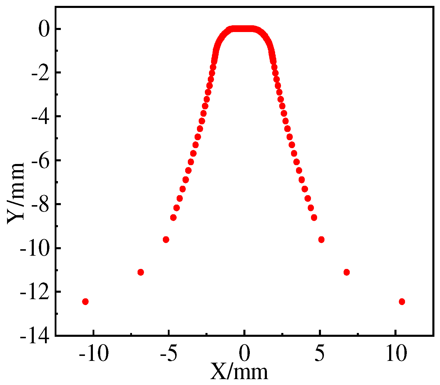
To investigate the influence of the grinding wheel’s installation angle on tooth surface distortion error, this study independently developed a virtual CNC gear machining center for axial modification using VERICUT9.1 software. The development process began with the 3D modeling of the machine bed and motion axes in UG, which were subsequently imported into VERICUT for virtual machine assembly. The development of the virtual prototype (Figure 5) proceeded as follows: The gear blank, with parameters from Table 1, is modeled in CREO. The cross-sectional profile of the grinding wheel (radius = 100 mm) is calculated (Figure 6) using the model from Section 2. This profile was then imported into CREO to create a 3D rotational model of the wheel. Finally, the G-code for simulating the axial modification and grinding was generated based on Equations (13) and (14).

Table 1. Parameters of Gear to be processed.

Gear Parameters	Symbol	Unit	Value	Gear Parameters	Symbol	Unit	Value
Number of teeth	$Z$	/	42	Helical angle	$\beta$	$\circ$	21.5
Normal modulus	$M_n$	mm	4	Base circle diameter	$d_b$	mm	168.1555
Normal pressure angle	${\alpha }_n$	°	20	Addendum Circle Diameter	$d_a$	mm	188.564
Addendum Coefficient	$h_a^{\ast }$	/	1	Axial modification amount	$\lambda$	µm	30
Tooth width	$B$	mm	35	Headspace coefficient	$c^{\ast }$	/	0.25

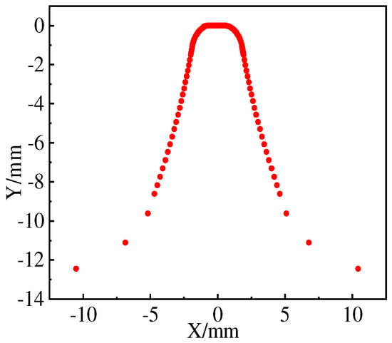
Figure 6. Profile of grinding wheel for gear to be machined.

5.2. Path Planning for Grinding Wheel Tool Processing

The axial double-sided modification process necessitates a variation in center distance, corresponding to the Y-axis linkage amount. With a specified modification of 30 μm, the procedure begins with the GW spindle rotation. The B-axis is rotated to set the wheel at the installation angle ${69.8549}^{°}$, and the X-axis positions the GW at the feed point. The Y-axis is then moved to tangency with the gear blank, followed by a retraction of 9 mm in its negative direction and an X-axis feed of 1.75 mm. The A-axis linkage angle, as derived from Equation (20), is 0.4374°. The center distance variation along the tooth width, representing the Y-axis linkage as per Equation (14), is listed in Table 2.

$$A={\displaystyle \frac{360\times \Delta L\times \sin \beta }{\pi \times M_n\times Z}}={\displaystyle \frac{360\times 1.75\times \sin {21.5}^{\circ }}{\pi \times 4\times 42}}={0.4374}^{\circ }$$

(20)

Table 2. Variation in the grinding wheel center distance.

Tooth Width/mm	Theoretical Axial Modification Value/mm	Variation in the Grinding Wheel Center Distance/mm
−17.5	0.03	0.082348084
−15.75	0.0243	0.066701948
−14	0.0192	0.052702774
−12.25	0.0147	0.040350561
−10.5	0.0108	0.02964531
………	………	………
0	0	0
………	………	………
10.5	0.0108	0.02964531
12.25	0.0147	0.040350561
14	0.0192	0.052702774
15.75	0.0243	0.066701948
17.5	0.03	0.082348084

5.3. Tooth Flank Measurement Path Planning

Upon completion of the machining process, a dedicated probe within VERICUT is utilized to measure the modified tooth flank. The probe parameters are listed in Table 3. In accordance with international standards [26], the actual evaluation range for tooth trace accuracy is defined as 90% of the total tooth width (1.75~33.25 mm). Let L8 denote the A-axis rotation angle when the probe contacts the left flank, and L9 the corresponding angle for the right flank. The median value for automatic alignment can then be expressed as $A=\left(L9+L8\right)/2$. Given a measured distance of 155.5 mm from the tool holder’s lower end face to the workpiece origin, the corresponding Y-axis position that brings the probe center into coincidence with the workpiece axis is calculated as 95.5 mm. After executing the G-code and rotating the A-axis, the measured rotation angle upon contact with the left flank is L8 = 68.4867°, and with the right flank L9 = 66.7697°. The resulting automatic alignment angle was therefore determined to be A = 67.6282°.

Table 3. Probe Parameters.

Parameter	Unit	Value/Coordinate
Probe radius	mm	1.5
Measuring rod diameter	mm	2
Automatic alignment of cutter point coordinates	/	(0, 0, −112.3)
Automatic clamping point coordinates	/	(0, 0, −0.8)
Hilt Length	mm	50
Hilt diameter	mm	50
Distance from the bottom end of the cutter to the center of the ball	mm	60

The measurement procedure consists of the following steps: (1) Position the X-axis at the left end of the tooth width and rotate the A-axis to the automatic alignment position; (2) Set the measurement circle radius from 87 mm to 93 mm and move the Y-axis to place the probe ball center at 35.5 mm; (3) Execute the G-code to record the A-axis angle upon probe contact; (4) Return the gear to the center and move the X-axis 1.75 mm left to collect data at the next point; (5) Repeat this cycle for all left flank sampling points; (6) Retract the probe along the Y-axis to a safe position; (7) Perform a symmetrical procedure to inspect the right tooth flank.

5.4. Axial Modification Tooth Flank Machining Result

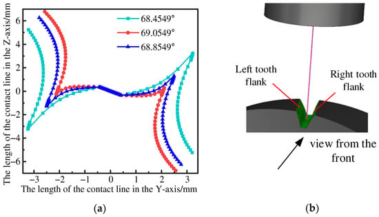
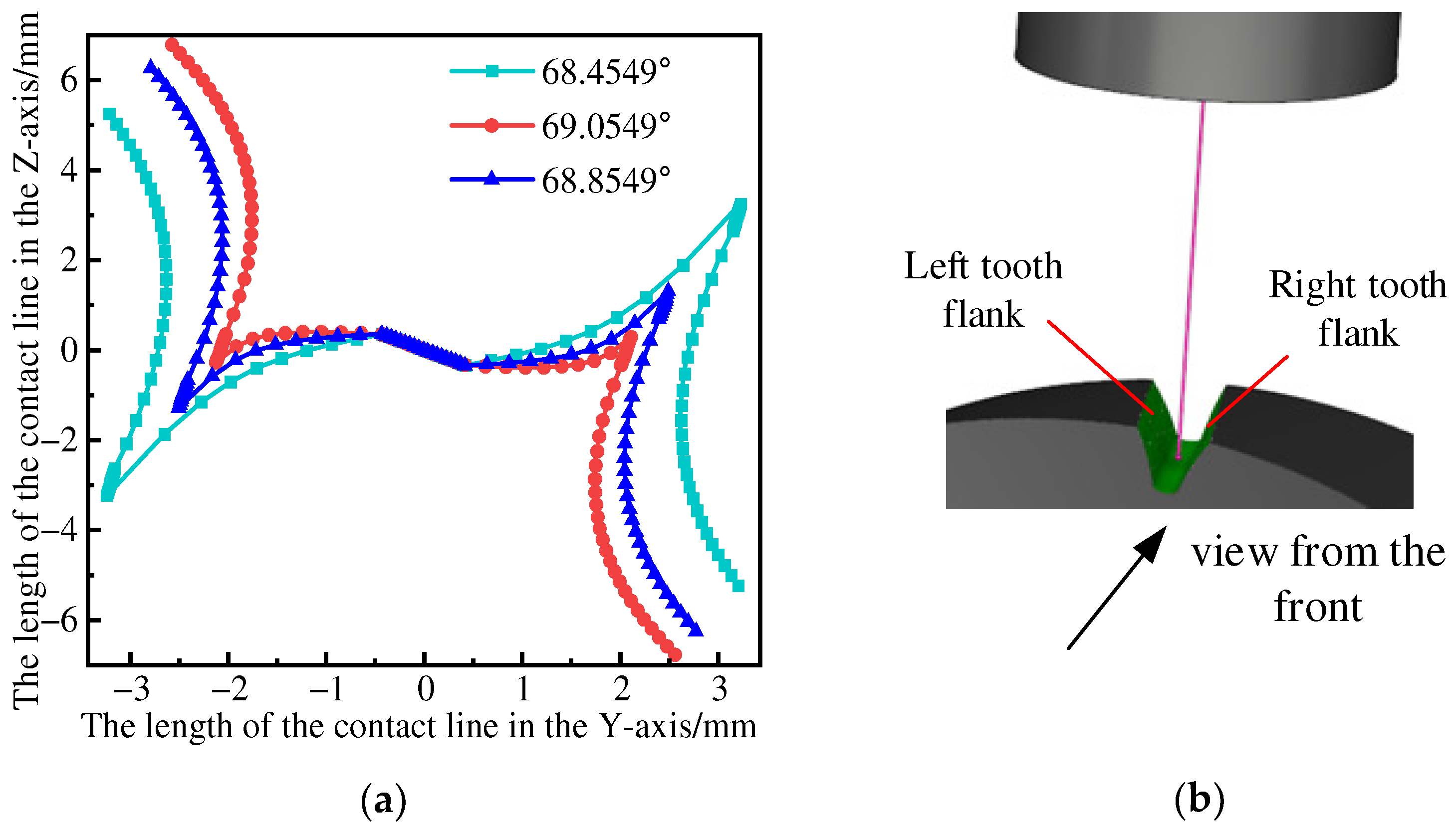
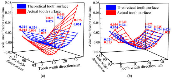
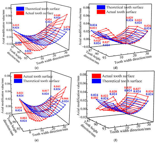
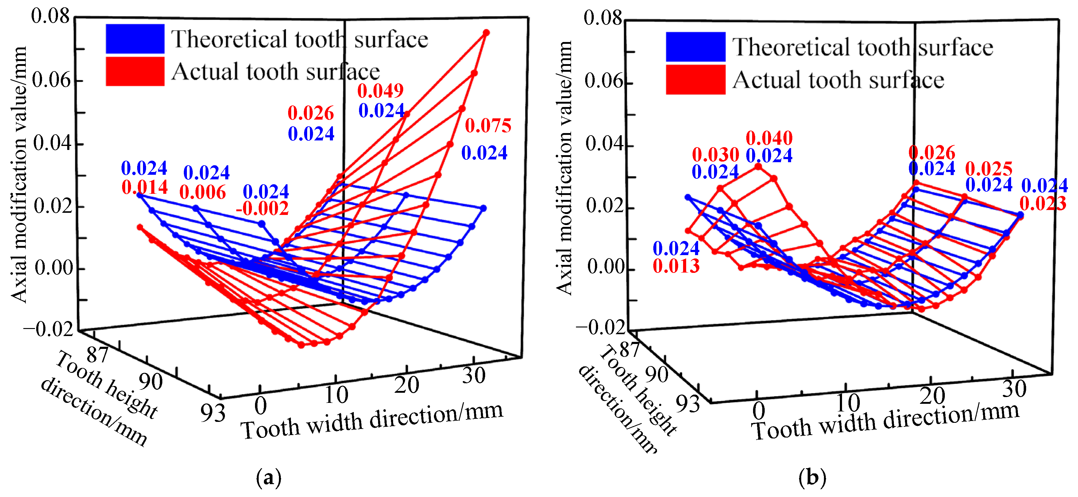
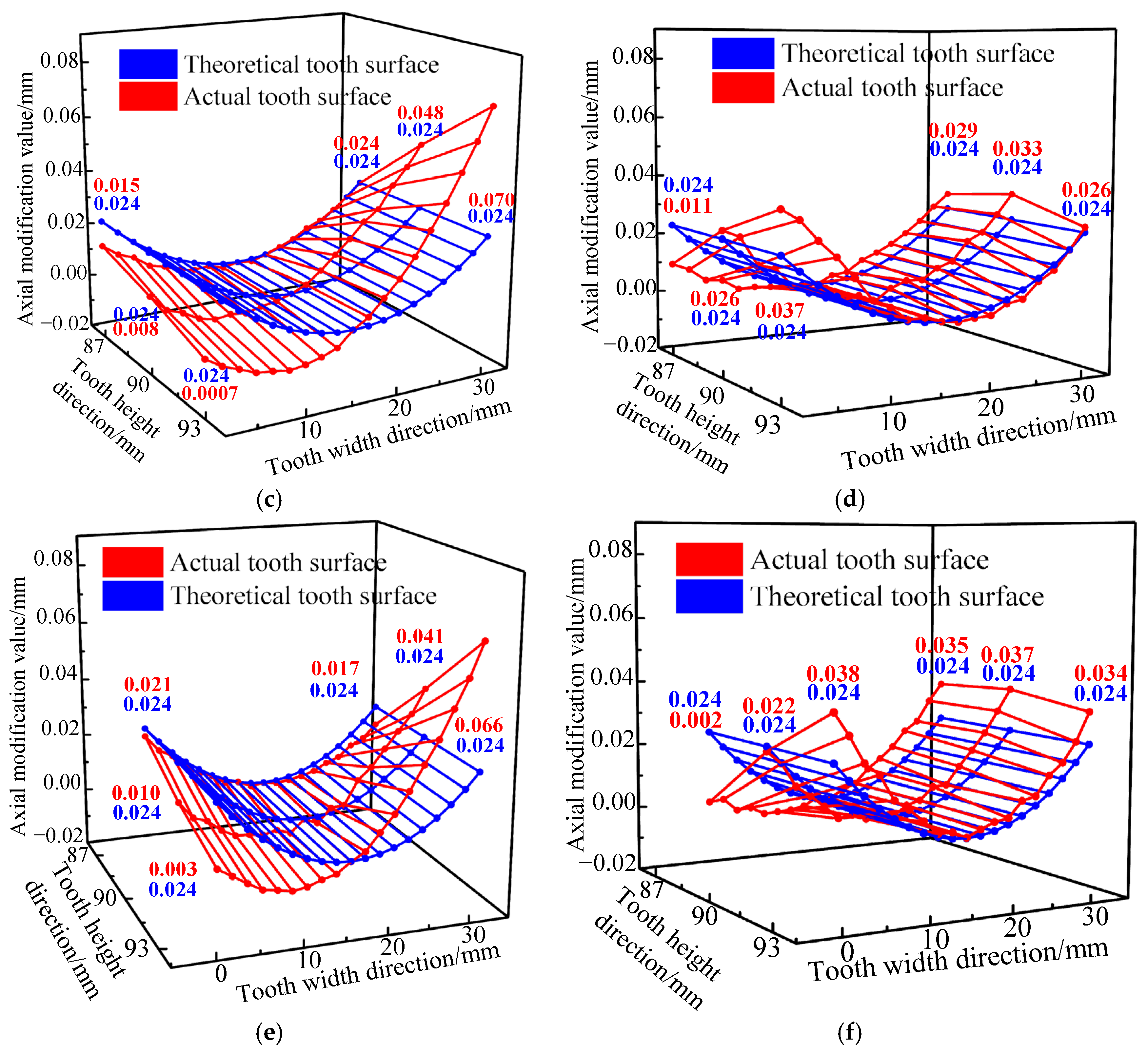
The grinding wheel installation angles are set to 69.0549°, 68.8549°, and 68.4549°, respectively, to perform axial modification and form-grinding processing. The resulting CL profile and virtual measurement schematic diagram are illustrated in Figure 7. Three sectional measurements are taken along the tooth height direction, with 19 measurement points distributed along the tooth direction and a measurement range of [1.75, 33.25]. Based on Equations (15)–(19), the tooth direction modification amount for any cross-section along the tooth width direction can be calculated. The processed tooth flank results are presented in Figure 8.

Figure 7. Contact line morphology under different GWIA and Virtual measurement schematic diagram. (a) Contact line morphology under different GWIA. (b) Virtual measurement.

Figure 8. The processing results of the tooth flank under different GWIA: (a) GWIA 69.0549° left tooth flank distortion error; (b) GWIA 69.0549° right tooth flank distortion error; (c) GWIA 68.8549° left tooth flank distortion error; (d) GWIA 68.8549° right tooth flank distortion error; (e) GWIA 68.4549° left tooth flank distortion error; (f) GWIA 68.4549° right tooth flank distortion error.

Figure 8 reveals a pronounced effect of the GWIA on tooth flank twisting. The twisting error shows a monotonic decrease with a smaller installation angle, underscoring the necessity of GWIA optimization for accuracy enhancement. Complementary to this, the axial modification curve also offers a viable pathway for precision improvement [27].

6. Tooth Flank Distortion Optimization Technology

6.1. Grinding Wheel Installation Angle and Contact Line Optimization Technique

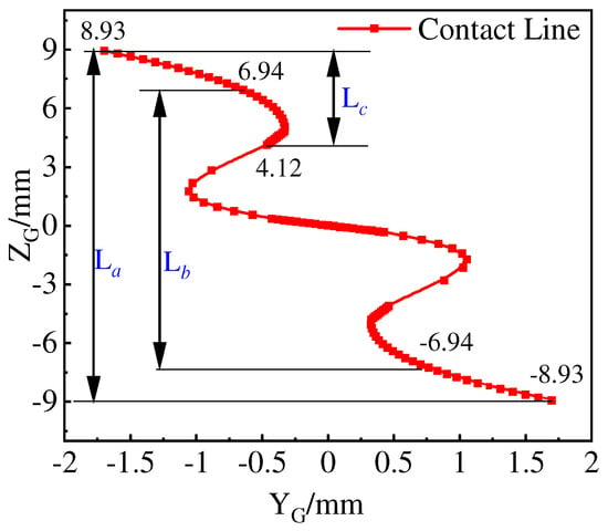
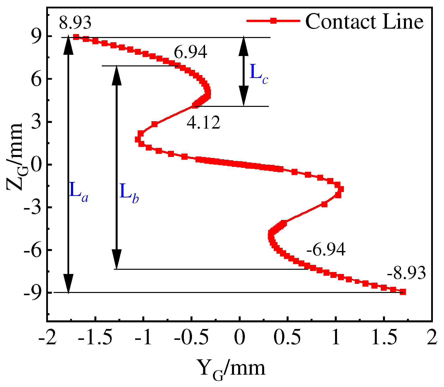
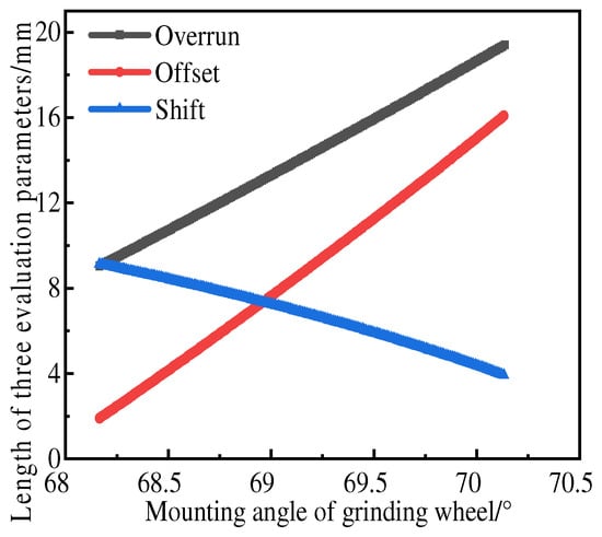
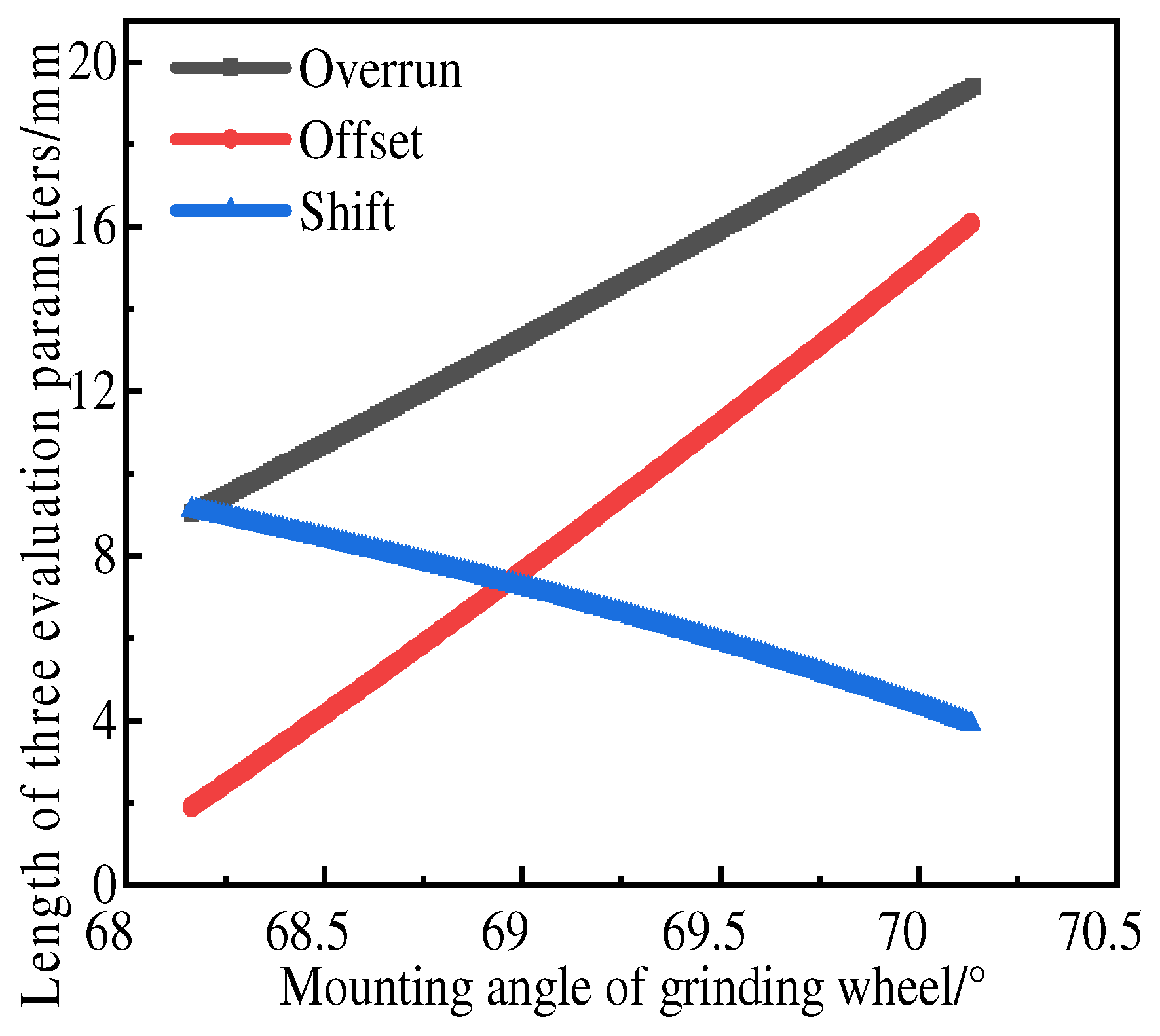
During actual gear grinding, the grinding wheel and the workpiece remain tangent along their contact line. A schematic representation of the contact line geometry in a planar view is provided in Figure 6. Evaluation of the contact line is typically based on three key parameters: overrun, offset, and shift, which correspond, respectively, to $L_a$, $L_b$, $L_C$ in Figure 9. The overtravel refers to the projection lengths of the first and last points on the contact line in $Z_G$ directions. It mainly affects the processing efficiency. The smaller the overrun, the higher the processing efficiency. Offset is defined as the projected distance, along the designated directions, between the intersection points of the reference circle with the left and right tooth flanks and their corresponding contact lines. It indicates the degree of asymmetry in the contact force distribution between the grinding wheel and the two flanks. A smaller offset value generally correlates with reduced grinding vibration. Shift describes the inclination of the contact line relative to a single tooth flank, primarily influencing the severity of tooth flank distortion. The variation trends of these three evaluation parameters with respect to the GWIA are illustrated in Figure 10. As the installation angle increases, both overrun and offset show a gradual increase, whereas shift exhibits a decreasing trend. Hence, by optimizing the GWIA, an optimal contact pattern can be achieved, thereby minimizing tooth flank distortion error.

Figure 9. Schematic diagram of the contact line.

Figure 10. Variation rule of evaluation parameters with the installation angle of the grinding wheel.

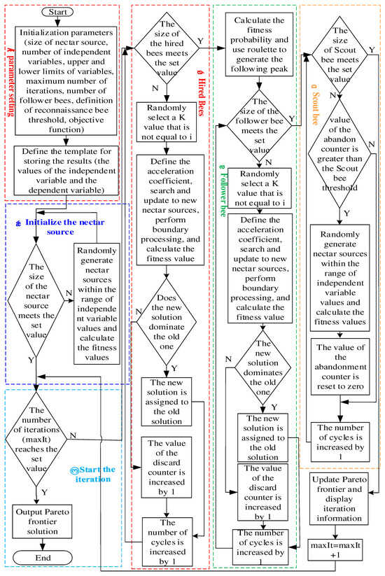
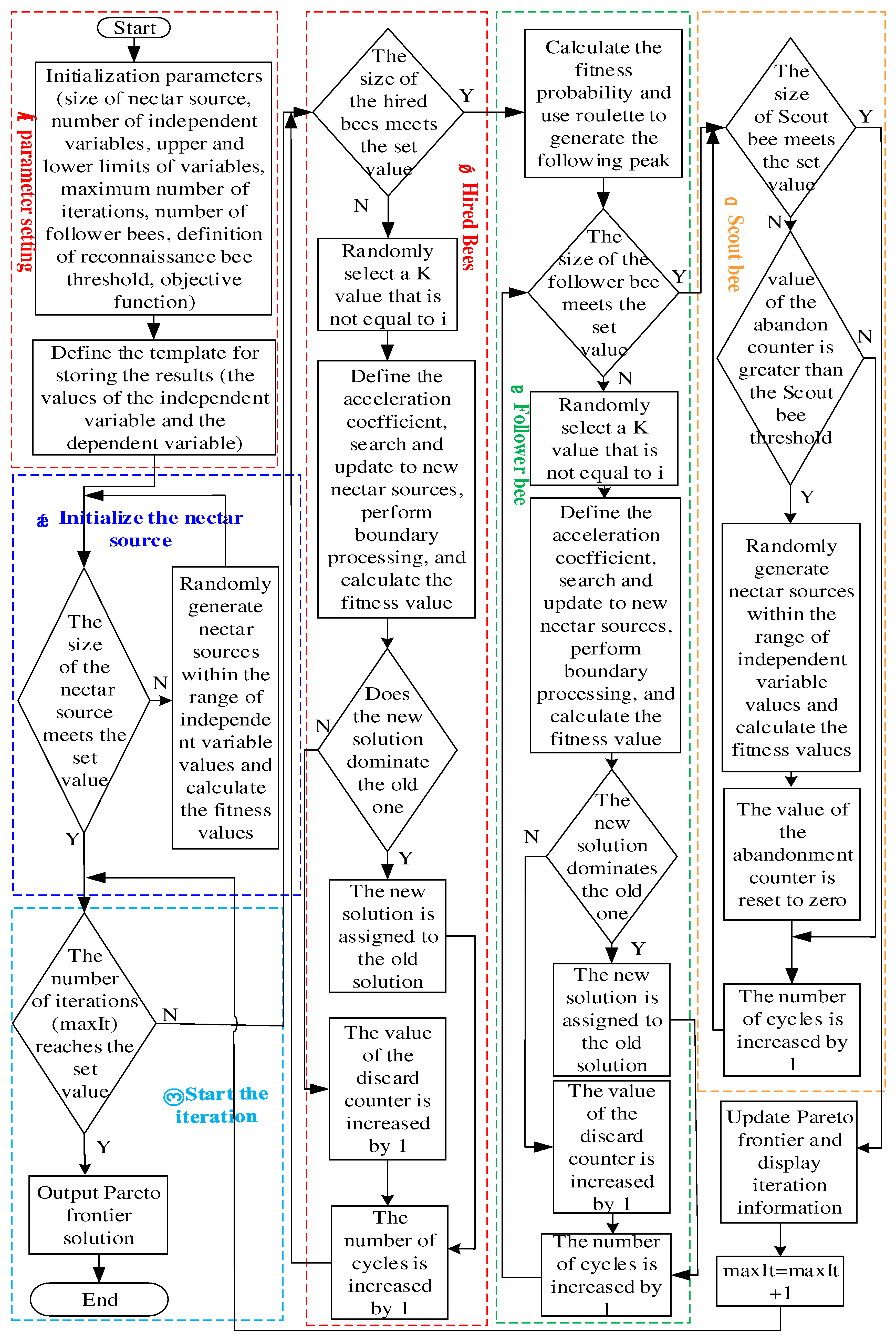
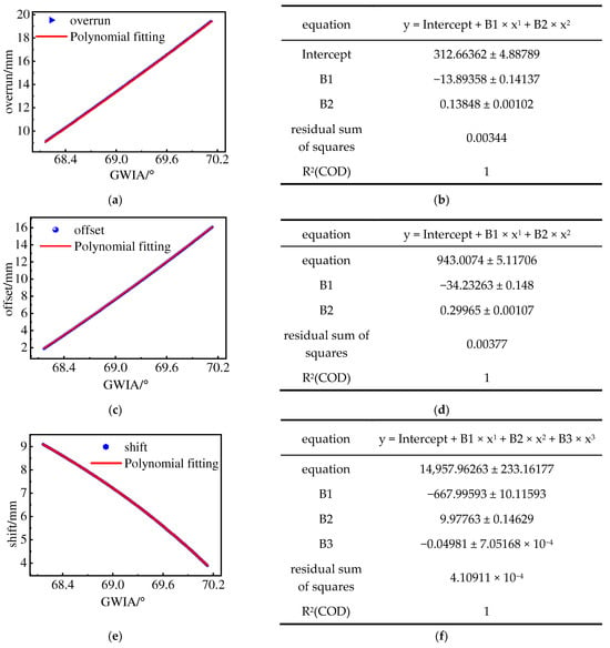
The regression equations of the GWIA with the overrun, offset, and shift are obtained by using the polynomial fitting method. The Artificial Bee Colony algorithm (ABC) is a swarm intelligence optimization algorithm developed by imitating the foraging behavior of bees. It has the characteristic of having few parameters. This algorithm achieves global optimization through the collaborative search mechanism of leading bees, following bees, and scout bees. The core elements include food sources (candidate solutions), employed bees (leading bees), and unemployed bees (scout bees/following bees). It updates the solution set using a greedy selection strategy and a roulette wheel probability mechanism. Based on the regression equation, a multi-objective optimization model is constructed. This model treats the GWIA as the optimization variable, with the objective of minimizing overrun, offset, and shift. The solution yields the optimal installation angle, which, when substituted into Equation (5), provides the optimized contact line. The specific steps of this process are summarized in the flowchart of Figure 11.

Figure 11. Schematic diagram of the artificial bee colony algorithm.

6.2. The Axial Modification Curve Optimization Technique

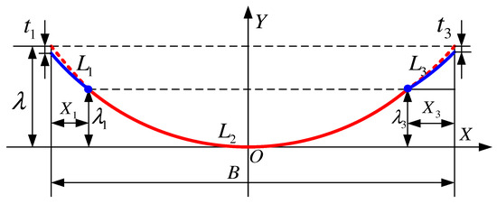
As illustrated in Figure 4b, the conventional axial modification curve follows a full-tooth-width drum-shaped profile, where the maximum distortion error typically occurs near the tooth tip or root regions at both end faces. However, since actual gear meshing requires the load to be uniformly distributed across the central region of the tooth width, a full-tooth-width drum modification is often unnecessary. In this study, the axial modification curve is optimized using a composite of three conical curve segments, as depicted in Figure 12. The resulting optimized profile comprises these three distinct sections. $L_2$ is the original modification curve, and the equation of the modification curve is shown in Equation (13). $L_1$ and $L_3$ are another modification curve. The position from the left end face of the gear is $X_1$, modification amount is ${\lambda }_1$. The difference in modification amounts between $L_1$ and $L_2$ on the left end face is $t_1$. At position $X_3$ from the right end face of the gear, the modification amount is ${\lambda }_3$, and the difference in modification amounts between $L_2$ and $L_3$ on the right end face is $t_3$.

Figure 12. The axial modification curve after optimization.

The mathematical expression of the optimized piecewise modification curve is:

$$\left\{\begin{array}{ll}Y(x)={\displaystyle \frac{4\lambda }{B^2}}{x}^2+{\displaystyle \frac{({\lambda }_1+t_1)-\frac{4\lambda }{B^2}{(-\frac{B}{2}+X_1)}^2}{X_1}}x-t_1+{\displaystyle \frac{B}{2}}\cdot {\displaystyle \frac{({\lambda }_1+t_1)-\frac{4\lambda }{B^2}{(-\frac{B}{2}+X_1)}^2}{X_1}}\hfill & (-{\displaystyle \frac{B}{2}}\le x<-{\displaystyle \frac{B}{2}}+X_1)\hfill \\ Y(x)={\displaystyle \frac{4\lambda }{B^2}}{x}^2\hfill & (-{\displaystyle \frac{B}{2}}+X_1\le x<{\displaystyle \frac{B}{2}}-X_3)\hfill \\ Y(x)={\displaystyle \frac{4\lambda }{B^2}}{x}^2+{\displaystyle \frac{\frac{4\lambda }{B^2}{(\frac{B}{2}-X_3)}^2-({\lambda }_3+t_3)}{X_3}}x-t_3-{\displaystyle \frac{B}{2}}\cdot {\displaystyle \frac{\frac{4\lambda }{B^2}{(\frac{B}{2}-X_3)}^2-({\lambda }_3+t_3)}{X_3}}\hfill & ({\displaystyle \frac{B}{2}}-X_3\le x<{\displaystyle \frac{B}{2}})\hfill \end{array}\right.$$

(21)

According to Equation (13), the axial modification amount of each point of the optimized modification curve can be obtained. According to Equation (14), the corresponding variation of the center distance of the GW can be calculated.

7. Simulation Results and Experimental Verification

7.1. The Result of Axial Modification Before Optimization

The machining sequence is initiated by starting the GW spindle and setting the GWIA to 69.8549° via the B-axis. The GW is then positioned at the entry point by the X-axis, and the Y-axis is moved to establish tangency with the gear blank, followed by a 9 mm retraction. The tooth flank modification is completed by executing the G-code, which synchronizes a 1.75 mm axial feed (X-axis) with a 0.4374° rotation (A-axis).

The measurement procedure for the left flank is as follows: (1) Position the A-axis at the left tooth width and rotate it to the automatic centering position (67.6282°); (2) Set the measurement circle radius from 87 mm to 93 mm and move the Y-axis to place the probe center at 35.5 mm; (3) Execute the G-code to record the A-axis angle upon probe contact; (4) Return the gear to the center and move the X-axis 1.75 mm left to collect the next point’s data; (5) Repeat steps (3) and (4) cyclically until all sampling points on the left flank are measured.

After the probe retracts along the Y-axis to a safe position, the same procedure is repeated to measure the right flank. The modification amount at any cross-section along the tooth width can then be calculated using Equations (14)–(19). The virtual machining results for the left and right flanks of the tooth slot are presented in Figure 13.

Figure 13. Optimization of axial modification simulation for the left and right flanks of the preceding tooth groove: (a) Simulated tooth flank after axial modification—left flank; (b) Simulated tooth flank after axial modification—right flank.

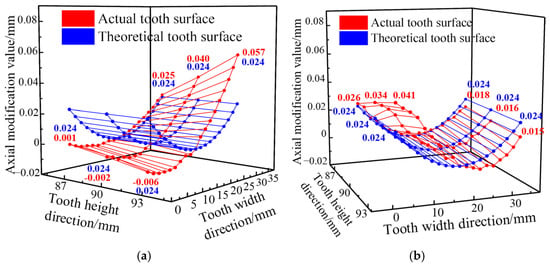
To ensure full drum-shaped modification at the reference circle, the grinding wheel is fed along this circle. However, it can be observed that after the right flank has been fully modified, the contact line corresponding to the left flank still lies within the tooth flank. As a result, a certain segment along the tooth width remains unprocessed, potentially leading to lateral scoring marks on the tooth flank. This issue may be mitigated by appropriately extending the axial modification curve. Both flanks exhibit diagonal distortion after modification, with the left flank showing more pronounced distortion than the right. Prior to optimization, the maximum axial modification error reached 33 μm on the left flank, compared to 17 μm on the right flank.

7.2. Simulation Results of Optimized Axial Modification

To mitigate tooth flank distortion and improve gear transmission performance in axial modification processes, this study first applies polynomial fitting to obtain regression equations for the grinding wheel installation angle (GWIA) with respect to overrun, offset, and shift (Equation (28)). The expression for the output of the polynomial is set as

$$y=a_0+a_{1}x+a_2{x}^2+a_3{x}^3+\dots +a_n{x}^n$$

(22)

The sample data of the independent variable and the dependent variable can be expressed as

$$\left\{\begin{array}{l}x={[x_1,x_2,x_3,x_4,\dots ,x_m]}^T\\ y={[y_1,y_2,y_3,y_4,\dots ,y_m]}^T\end{array}\right.$$

(23)

Substituting Equation (23) into Equation (22) yields:

$$\left\{\begin{array}{c}{y}_1=a_0+a_1{x}_1+a_2{x}_1^2+\dots +a_n{x}_1^n\\ y_2=a_0+a_1{x}_2+a_2{x}_2^2+\dots +a_n{x}_2^n\\ ⋮\\ y_m=a_0+a_1{x}_m+a_2{x}_m^2+\dots +a_n{x}_m^n\end{array}\right.$$

(24)

Equation (24) can be transformed into matrix form as

$$\left(\begin{array}{c}{y}_1\\ y_2\\ ⋮\\ y_m\end{array}\right)=\left(\begin{array}{ccccc}1& x_1& x_1^2& \dots & x_1^n\\ 1& x_2& x_2^2& \dots & x_2^n\\ ⋮& ⋮& ⋮& \dots & ⋮\\ 1& x_m& x_m^2& \dots & x_m^n\end{array}\right)\left(\begin{array}{c}{a}_0\\ a_1\\ ⋮\\ a_n\end{array}\right)$$

(25)

Equation (25) can be expressed as:

$$y=Aa$$

(26)

$$a=A^{-1}y$$

(27)

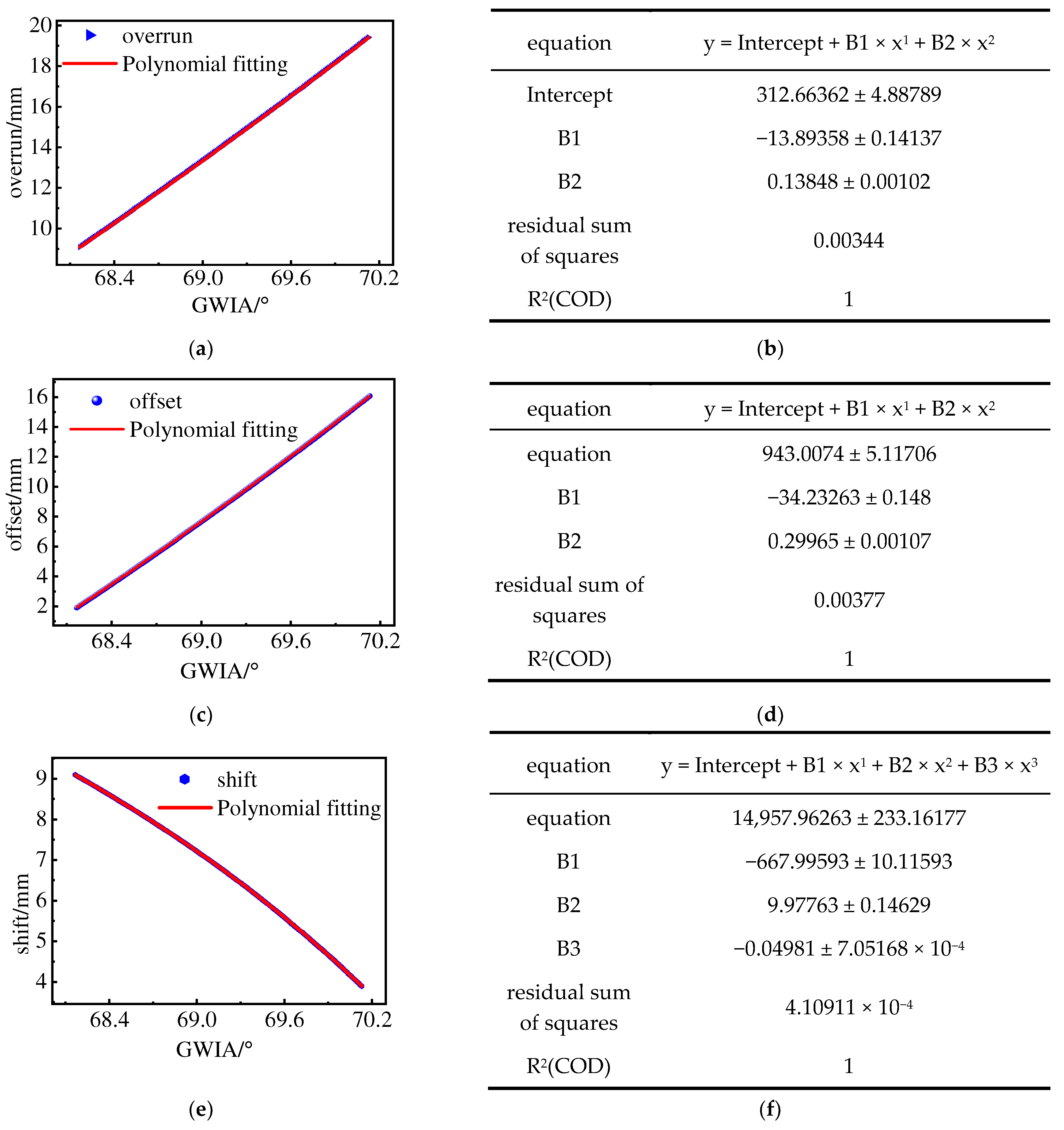
According to Equation (27), the regression equations of the grinding wheel installation angle with the overrun, amount, offset amount and shift position can be derived. In this paper, the Origin2026 software is used for polynomial fitting, and the fitting results are shown in Figure 14.

Figure 14. Result of Polynomial Fitting for Origin. (a) Overrun Polynomial fitting. (b) Overrun polynomial fitting curve equation. (c) Offset Polynomial fitting. (d) Offset polynomial fitting curve equation. (e) Shift Polynomial fitting. (f) Shift polynomial fitting curve equation.

Subsequently, a multi-objective optimization model is established using the ABC algorithm, treating Equation (28) as the objective function and considering the non-interference range of GWIA. The algorithm is configured with 100 nectar sources, 100 maximum iterations, an acceleration coefficient of 1, 100 follower bees, and a scout bee threshold of 60. The corresponding evaluation parameters for the optimized installation angle and contact line are listed in Table 4.

$$\left\{\begin{array}{l}{L}_a(\theta )=0.13848{\theta }^2-13.89358\theta +312.66362\hfill \\ L_b(\theta )=0.29965{\theta }^2-34.23263\theta +943.0074\hfill \\ L_C(\theta )=-0.04981{\theta }^3+9.97763{\theta }^2-667.99593\theta +14957.96263\hfill \end{array}\right.$$

(28)

Table 4. Comparison of the GWIA, CL and distortion error prior to and subsequent to optimization.

	Mounting Angle of Grinding Wheel/°	Overrun/ mm	Offset/ mm	Shift/ mm	Maximum Distortion Error of Left Tooth Flank/µm	Maximum Distortion Error of Right Tooth Flank/µm
pre-optimization	69.8549	17.8539	13.8773	4.8058	33	17
post-optimization	68.2509	9.46063	2.40851	8.9201	17	12

According to the optimization method of the axial modification curve described in Section 4.2, the modification curve along the tooth width direction is divided into three sections. As shown in Figure 12, at position $X_1=3.5 \mathrm{mm}$, the modification amount is ${\lambda }_1=19.2 \mathrm{\mu m}$, and the difference in modification amounts between $L_1$ and $L_2$ on the left end face is $t_1=5 \mathrm{\mu m}$. At position $X_3=3.5 \mathrm{mm}$ from the right end face of the gear, the modification amount is ${\lambda }_3=19.2 \mathrm{\mu m}$, and the difference in modification amounts between position $L_2$ and position $L_3$ on the right end face is $t_3=5 \mathrm{\mu m}$. Substituting the above parameters into Equation (21) can yield the tooth flank equation after the modification curve optimization:

$$\left\{\begin{array}{l}Y(x)={\displaystyle \frac{0.12}{{35}^2}}{x}^2+{\displaystyle \frac{5\times {10}^{-3}}{3.5}}x+0.02\hspace{1em} (-17.5\le x<-14)\hfill \\ Y(x)={\displaystyle \frac{0.12}{{35}^2}}{x}^2\hspace{1em}\hspace{1em}\hspace{1em}\hspace{1em}\hspace{1em}\hspace{1em}\hspace{1em} (-14\le x\le 14)\hfill \\ Y(x)={\displaystyle \frac{0.12}{{35}^2}}{x}^2-{\displaystyle \frac{5\times {10}^{-3}}{3.5}}x+0.02\hspace{1em} (14<x\le 17.5)\hfill \end{array}\right.$$

(29)

Based on Equation (29), the modified amount at any position along the tooth width after optimization can be computed. Subsequently, Equation (14) is applied to determine the corresponding variation in the center distance. The G-code for the grinding process is then updated to adjust the linkage parameters governing the GWIA and center distance. The optimized grinding wheel profile is derived from the refined spatial contact line using the mathematical model presented in Section 2. Following the pre-optimized form grinding tool path, a grinding test for helical gear axial modification is conducted. Gear angle measurements are recorded, and the axial modification value at any vector diameter is calculated using Equations (15)–(19). The post-optimization machining results for the left and right tooth flanks are shown in Figure 13.

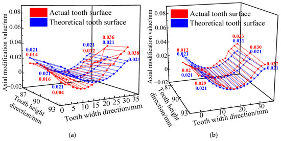
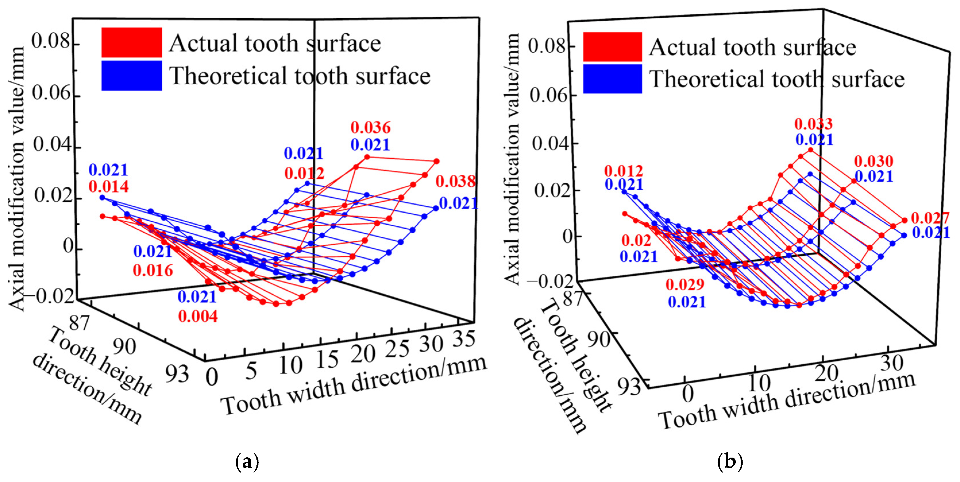
It can be seen from Figure 15 that the maximum axial modification error after the optimization of the left tooth flank is 17 $\mathrm{\mu m}$, and the maximum axial modification error after the optimization of the right tooth flank is 12 $\mathrm{\mu m}$. The distortion error of the left tooth flank is reduced by 48.5%, while that of the right tooth flank is reduced by 29.4%.

Figure 15. Simulated machining results of the optimized left and right flanks of the tooth groove: (a) Simulated axially modified flank—left flank; (b) Simulated axially modified flank—right flank.

7.3. Experimental Verification

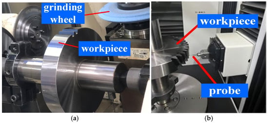
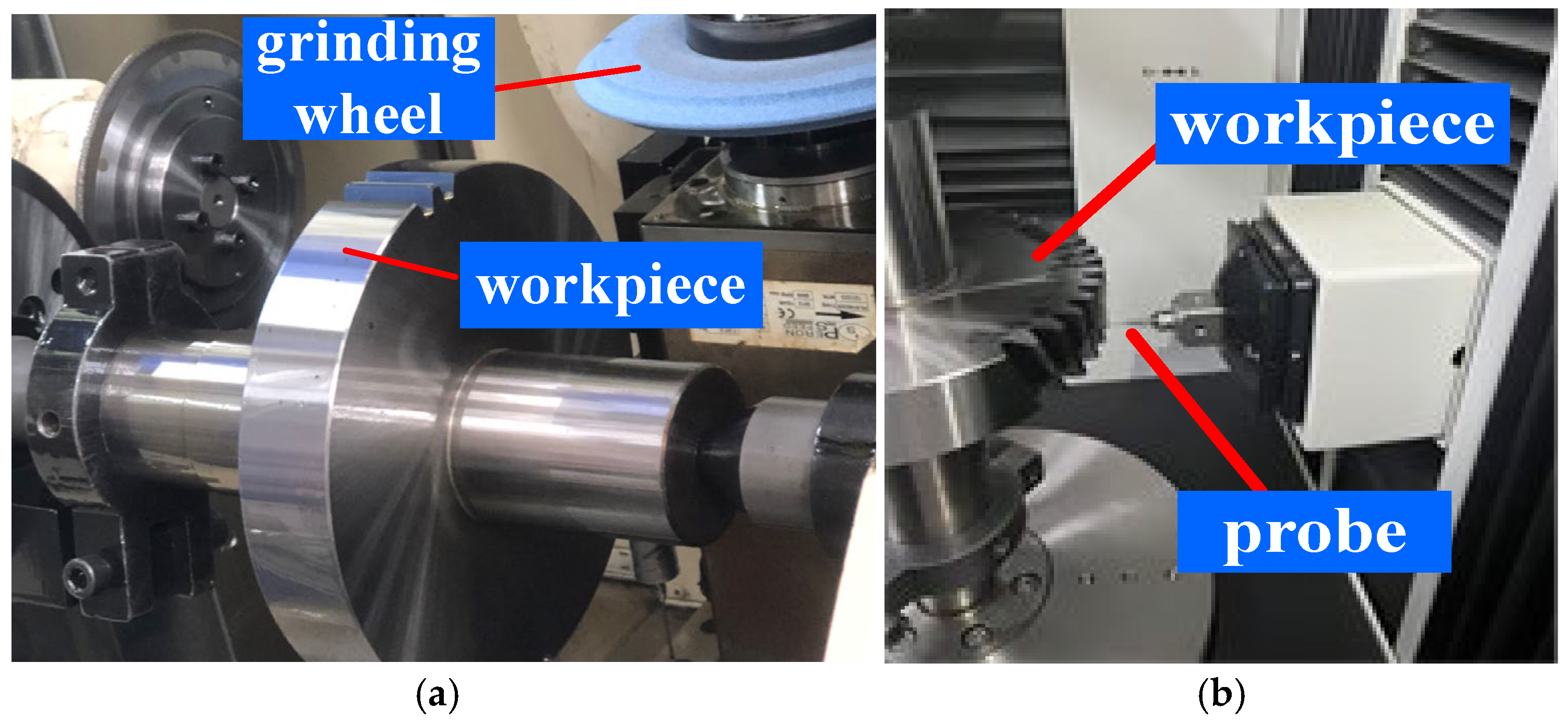
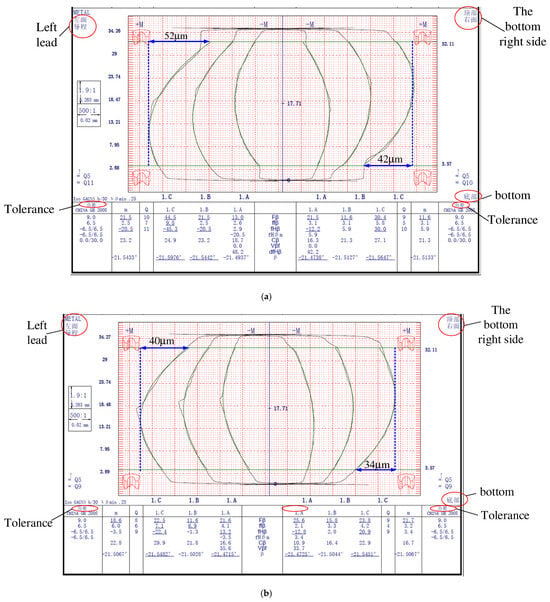
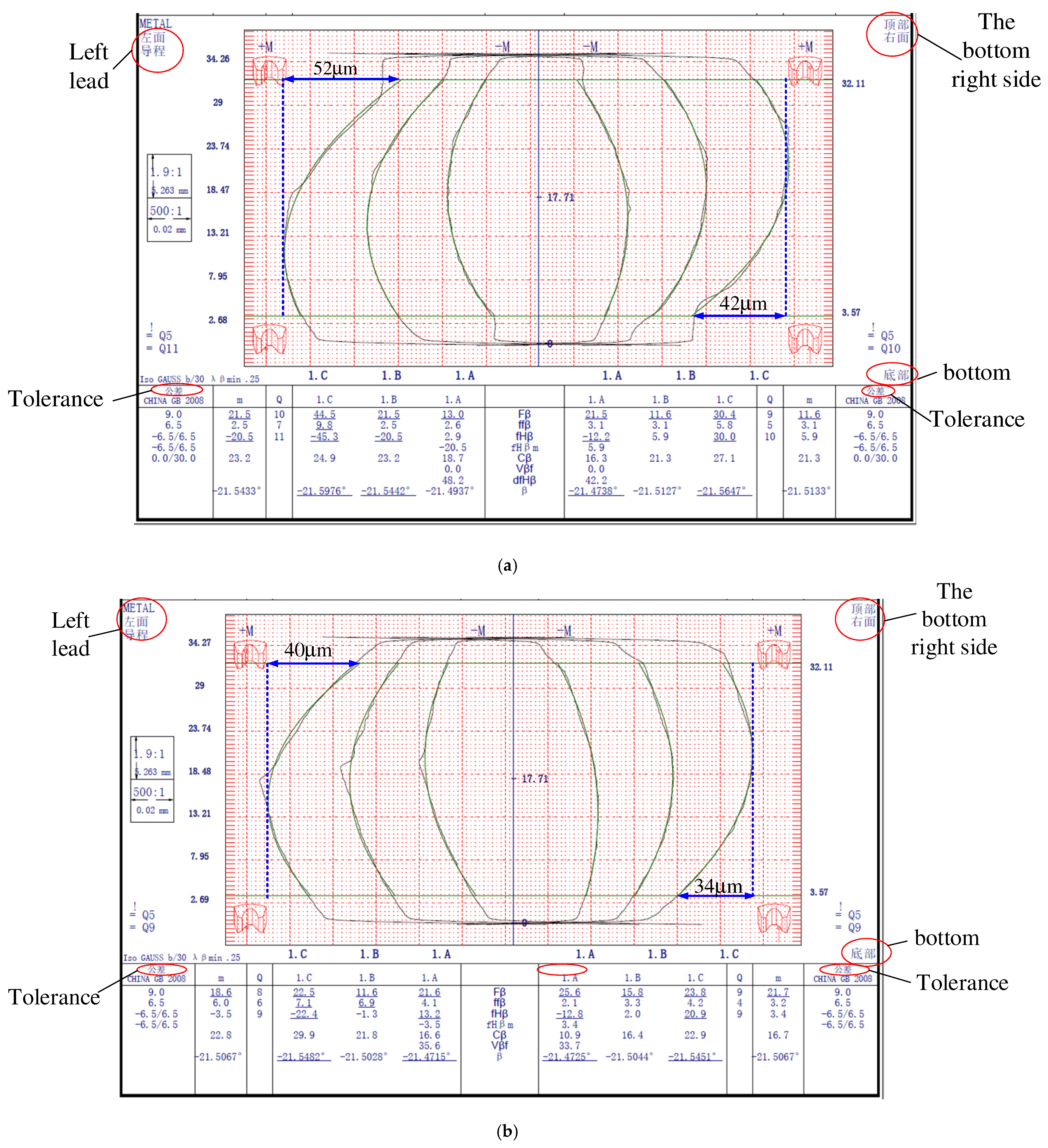
To substantiate the accuracy of the simulated axial modification grinding process, an experimental study is conducted using the L300G gear grinding machine. The grinding setup is illustrated in Figure 16a. The procedure begins with the tool moving −218.9269 mm. Subsequently, the B-axis rotates while the tool advances 30 mm in the positive X-direction, which marks the start of axial modification. A continuous X-axis movement of 6.524 mm is then executed. Theoretically, the contact line intersects with the reference circle on the tooth end face. Center distance modification is initiated based on the variation values provided in Table 2. Twenty grinding passes are performed along the tooth width to complete the axial modification process. The tooth flank is measured using the Gleason measuring equipment shown in Figure 16b, with results displayed in Figure 17a.

Figure 16. Helical gear forming grinding processing: (a) L300G grinding processing; (b) Gleason axial modification tooth flank measurement.

Figure 17. Optimize the measurement results of the tooth flank before and after axial modification. (a) Optimization of the modification for the front tooth flank measurement results. (b) Measurement results of the modified tooth flank in the optimized tooth direction.

The optimal grinding wheel installation angle, identified via the artificial bee colony algorithm, is 68.2509°. The corresponding variation in the center distance is calculated using Equation (14). The axial modification grinding is then carried out with a wheel feed rate of 1.75 mm per pass, distributed over 20 feeds across the tooth width. Flank measurements obtained using the Gleason instrument are presented in Figure 17b.

The involute helical gear after longitudinal crowning modification deviates from the geometric characteristics of standard gears. Therefore, this paper conducts a tooth surface quality evaluation based on the crowning modification amount. As shown in Figure 17, three typical sections along the tooth height direction are selected for measurement and analysis. The results indicate that the tooth surface twist error reaches its maximum in the tooth tip region. Before optimization, the measured machining twist errors on the left and right tooth surfaces are 28 μm and 18 μm, respectively. After optimization, these errors are reduced to 16 μm and 10 μm, representing reductions of 42.8% and 44.4%. Furthermore, the relative deviation between the experimentally obtained twist error after optimization and the simulation prediction results is controlled within approximately 10%, validating the effectiveness of the modification strategy and the accuracy of the modeling.

8. Conclusions

This paper takes the involute helical gear as the research object. Based on the principle of form-grinding, the mathematical models of the CL and the cross-section of the grinding wheel are established. The axial modification curve is designed, and the calculation method of the tooth direction drum shape at any cross-section along the tooth height direction is derived. The optimal GWIA and CL are solved by using the multi-objective optimization algorithm of artificial bee colony. The traditional axial modification curve is optimized in the form of a combination of three sections of a conic section. The conclusions are as follows:

(1)

Based on the principles of FG, this study establishes a mathematical model describing both the CL and the grinding wheel profile. Utilizing this model, an improved contact line and corresponding wheel cross-section are derived, furnishing a theoretical groundwork for the axial modification process in form grinding.

(2)

Due to the oblique projection of the CL onto the tooth flank, the modification depth near the tooth root is greater on the left end than on the right, while the modification at the tooth tip is more pronounced on the right end. Consequently, tooth flank distortion resulting from axial modification exhibits a diagonal pattern, with the distortion characteristics of the right flank mirroring those of the left in an opposing manner.

(3)

Taking the GWIA as the optimization variable, a multi-objective ABC algorithm is employed to determine the optimal installation angle and spatial contact line configuration. The conventional MC is enhanced using a composite profile consisting of three conic segments. Experimental trials conducted on an L300G gear grinding machine demonstrated a 48.5% reduction in distortion error on the left flank and a 29.4% reduction on the right flank after optimization. The discrepancy between simulated and experimental results is approximately 10%, indicating that the integrated optimization approach proposed in this study offers valuable insights for improving the accuracy of axial modification processes. After the teeth of the gears undergo profile modification, the tooth surfaces are no longer standard involute surfaces. In this paper, the criterion is based on the axial modification value, while in reference [28], the evaluation is made based on the torsion of the cross-section (Sα) and the torsion of the side profile (Sβ).

Although this study has effectively reduced the fundamental error of tooth flank distortion in helical gear axial modification, the axial modification curves on the left and right tooth flanks are not entirely symmetrical along the tooth width direction. Therefore, future research will focus on further investigating tooth flank distortion reduction techniques to minimize distortion errors and enhance the transmission performance of gears.

References

- He, K.; Li, G.L.; Du, Y.B.; Shang, N. A method for reducing tooth flank distortion in form grinding based on multi-axis additional motion optimization. Comput. Integr. Manuf. Syst. 2019, 25, 1946–1955. [Google Scholar] [CrossRef]
- Jiang, J.K.; Fang, Z.D.; Bian, X. Optimal design of longitudinal correction of double helical gear. J. Harbin Inst. Technol. 2013, 45, 86–92. [Google Scholar]
- Zhang, H.; Fang, C.G.; Guo, E.K.; Huang, X.T. Precision tooth direction modification of CNC forming gear grinding based on five-axis motion optimization. Comput. Integr. Manuf. Syst. 2014, 20, 3058–3065. [Google Scholar] [CrossRef]
- He, K.; Du, Y.B.; Li, G.L. Analysis of the principle error of the tooth flank in the form grinding of toothed modified helical gears. Comput. Integr. Manuf. Syst. 2018, 24, 1401–1410. [Google Scholar] [CrossRef]
- Guo, E.K.; Huang, X.T.; Fang, C.G.; Yuan, H. A contact line optimization method for improving the modification accuracy of the tooth direction of formed grinding teeth. Comput. Integr. Manuf. Syst. 2014, 20, 134–141. [Google Scholar] [CrossRef]
- Wang, H.L.; Deng, X.Z.; Yang, J.J.; Kai, X.; Su, J.X.; Chen, Q. Form grinding and testing of segmented topological modified gears. J. Aerosp. Power 2014, 29, 3000–3008. [Google Scholar] [CrossRef]
- Li, G.L.; Li, X.G.; Liu, F.; Sun, M.H. Optimization method of sand contour in topological modified gear with additional radial motion form grinding. J. Mech. Eng. 2011, 47, 155–162. [Google Scholar] [CrossRef] [Scilit]
- Su, Z.J.; Li, X.D.; Yin, X.M.; Jia, H.T.; Guo, F. The design of linear diagonal trimming of herringbone gears and the principle of forming grinding. J. Mech. Eng. 2023, 59, 121–129. [Google Scholar] [CrossRef] [Scilit]
- Li, Y.; Li, G.; Wang, Z.H.; Zhu, W.M. A form-grinding wheel optimization method for helical gears based on a PSO-SVM model. Precis. Eng.-J. Int. Soc. Precis. Eng. Nanotechnol. 2024, 88, 664–673. [Google Scholar] [CrossRef] [Scilit]
- Li, Y.; Wang, Z.; Liu, L.; Diao, X.W.; Zhu, X.Y. Analysis and optimization of the properties of the grinding contact line for form-grinding modified helical gears. Int. J. Adv. Manuf. Tech. 2022, 120, 403–413. [Google Scholar] [CrossRef] [Scilit]
- Wang, C. Multi-objective optimal design of modification for helical gear. Mech. Syst. Signal Process. 2021, 157, 107762. [Google Scholar] [CrossRef] [Scilit]
- Yao, X. Multi-objective optimization model of transmission error of nonlinear dynamic load of double helical gears. Nonlinear Eng. 2023, 12, 20220323. [Google Scholar] [CrossRef] [Scilit]
- Younes, E.B.; Changenet, C.; Bruyère, J.; Rigaud, E.; Perret-Liaudet, J. Multi-objective optimization of gear unit design to improve efficiency and transmission error. Mech. Mach. Theory 2022, 167, 104499. [Google Scholar] [CrossRef] [Scilit]
- He, K.; Wang, A.; Du, Y.B.; Yan, B.; Li, R.H. Optimization design of gear with lead modification considering the effect of twist error. J. Mech. Sci. Technol. 2024, 38, 5649–5659. [Google Scholar] [CrossRef] [Scilit]
- Zhou, S.M.; Zhang, D.H. Research on Multi-Objective Optimization of Helical Gear Shaping Based on an Improved Genetic Algorithm. Machines 2025, 13, 295. [Google Scholar] [CrossRef] [Scilit]
- Han, J.; Jiang, H.; Tian, X.Q.; Li, G.H.; You, T.F.; Xia, L. Topology modification method of generating gear grinding based on multi-axis linkage parameter optimization. Int. J. Adv. Manuf. Technol. 2022, 124, 449–466. [Google Scholar] [CrossRef] [Scilit]
- Shih, Y.P.; Chen, S.D. A flank correction methodology for a five-axis CNC gear profile grinding machine. Mech. Mach. Theory 2012, 47, 31–45. [Google Scholar] [CrossRef] [Scilit]
- Yuan, B.; Liu, G.; Yue, Y.G.; Liu, L.; Shen, Y.B. A novel tooth flank modification methodology for wide-faced double-helical gear pairs. Mech. Mach. Theory 2021, 160, 104299. [Google Scholar] [CrossRef] [Scilit]
- Rogkas, N.; Pelekis, M.; Manios, A.; Anastasiadis, A.; Vasileiou, G.; Tsoukalis, A.; Manopoulos, C.; Spitas, V. Design, Simulation and Multi-Objective Optimization of a Micro-Scale Gearbox for a Novel Rotary Peristaltic Pump. Micromachines 2023, 14, 2099. [Google Scholar] [CrossRef] [Scilit]
- Lin, T.J.; He, Z.Y. Analytical method for coupled transmission error of helical gear system with machining errors, assembly errors and tooth modifications. Mech. Syst. Signal Process. 2017, 91, 167–182. [Google Scholar] [CrossRef] [Scilit]
- Tian, X.Q.; Li, D.; Huang, X.Y.; Liu, H.J.; Han, J.; Xia, L. A topological flank modification method based on contact trace evaluated genetic algorithm in continuous generating grinding. Mech. Mach. Theory 2022, 172, 104820. [Google Scholar] [CrossRef] [Scilit]
- Yan, P.F.; Liu, H.; Gao, P.; Zhang, X.; Zhan, Z.B.; Zhang, C. Optimization of distributed axial dynamic modification based on the dynamic characteristics of a helical gear pair and a test verification. Mech. Mach. Theory 2021, 163, 104371. [Google Scholar] [CrossRef] [Scilit]
- Liu, Y.P.; Chen, Q.; Dong, C.B. Effect of Axial Modification on the Meshing Performance of Involute Beveloid Gear Pair. Appl. Sci. 2025, 15, 1321. [Google Scholar] [CrossRef] [Scilit]
- Gao, P.; Liu, H.; Yan, P.F.; Xie, Y.K.; Xiang, C.L.; Wang, C. Research on application of dynamic optimization modification for an involute spur gear in a fixed-shaft gear transmission system. Mech. Syst. Signal Process. 2022, 181, 109530. [Google Scholar] [CrossRef] [Scilit]
- Li, R.X. Principles and Calculations of Tool Design; Jiangsu Science and Technology Press: Nanjing, China, 1985. [Google Scholar]
- ISO. 1328 Cylindrical Gears—ISO System of Flank Tolerance Classification—Part 1: Definitions and Allowable Values of Deviations Relevant to Flanks of Gear Teeth, 2nd ed.; ISO: Geneva, Switzerland, 2013. [Google Scholar]
- Shen, M.; Hong, R.J.; Sun, X.M.; Xu, J.M. Based on inverse compensation to the modification curve tooth flank distortion. Mod. Mach. Tool Autom. Manuf. Tech. 2025, 5, 10. [Google Scholar] [CrossRef]
- Zhang, B.; Zhang, Y.; Zhang, L.; Li, Q.Y.; Wang, X.Y. Geometric Parameter Optimization for Axial Modification in Helical Gear Form Grinding. Machines 2024, 12, 657. [Google Scholar] [CrossRef] [Scilit]
Disclaimer/Publisher’s Note: The statements, opinions and data contained in all publications are solely those of the individual author(s) and contributor(s) and not of MDPI and/or the editor(s). MDPI and/or the editor(s) disclaim responsibility for any injury to people or property resulting from any ideas, methods, instructions or products referred to in the content. |
© 2026 by the authors. Licensee MDPI, Basel, Switzerland. This article is an open access article distributed under the terms and conditions of the Creative Commons Attribution (CC BY) license.