


Abstract
Motion planning for on-road autonomous driving requires generating locally accurate spatio-temporal trajectories over a finite horizon, while facing increasing uncertainty and interaction variability toward distant regions. However, most existing planners employ uniform planning accuracy along the horizon, which implicitly treats far-field predictions with the same fidelity as near-term execution. This uniform treatment often leads to unnecessary computational effort and reduced planning efficiency without improving near-field feasibility. This paper presents an economical motion planning framework that allocates planning accuracy according to the spatio-temporal distance from the ego vehicle. The framework preserves high-fidelity planning in the near field where execution is imminent, while progressively reducing resolution and solution depth in the far field where uncertainty dominates and replanning is expected. A two-stage architecture is adopted, combining a distance-aware search for coarse path and velocity generation with distance-sensitive numerical refinement that prioritizes near-field feasibility under receding horizon execution. The simulation results demonstrate improved computational efficiency and planning reliability compared with uniform resolution baselines. Real-world experiments validate the stable online replanning performance in dynamic environments.
1. Introduction
The objective of autonomous driving on urban roads is to generate safe, comfortable trajectories that guide vehicles from their current states to desired states within dynamically evolving environments [1]. Compared with low-speed, unstructured scenarios [2], motion planning on urban roads is more challenging [3]. On-road environments involve dynamic interactions with multiple traffic participants whose future behaviors are inherently uncertain and hard to predict [4]. This uncertainty places stringent demands on the trajectory planner: trajectories must be feasible in real time, remain stable under dynamic conditions, and stay near-optimal with respect to comfort and safety [5].
Trajectory planning for autonomous driving casts vehicle motion as a constrained optimization problem [6], in which a maneuver is selected by minimizing a cost function subject to spatio-temporal constraints imposed by road geometry, vehicle kinematics, and obstacle avoidance [7]. In practice, these constraints are tightly coupled and evolve continuously over the planning horizon. Even on straight roads, the presence of moving obstacles requires careful treatment of collision-avoidance constraints in both time and space [8]. As road curvature becomes more pronounced, the planning problem is further complicated by the strong coupling between roadway geometry and vehicle kinematics [9]. Moreover, unlike low-speed scenarios where braking can serve as an effective fallback [10], high-speed driving cannot rely on abrupt deceleration without risking rear-end collisions. As a result, beyond kinematic feasibility and collision safety, timely computation emerges as a critical requirement for on-road motion planning [11].
Most existing motion planners for on-road autonomous driving allocate computational resources uniformly across the spatio-temporal planning horizon. Such designs implicitly assume that motion states and environmental information are equally reliable at all distances and future times. In practice, however, perception accuracy and interaction predictability degrade with both distance from the ego vehicle and prediction horizon. Near-field regions are characterized by dense and reliable information and imminent execution, whereas far-field regions are dominated by increasing uncertainty.
Treating near-field and far-field regions with uniform planning fidelity therefore leads to the inefficient use of computational resources and limits real-time responsiveness [12]. To address this mismatch, this paper proposes an economical motion planning strategy that explicitly allocates spatio-temporal resolution according to distance ahead of the ego vehicle. Higher planning fidelity and computational effort are concentrated in the near field, while planning resolution is progressively reduced farther along the horizon. The proposed strategy is agnostic to the underlying planning algorithm and can be embedded into a broad range of planning frameworks.
The remainder of this paper is organized as follows. Section 2 reviews the related literature. Section 3 states the concerned on-road trajectory planning problem. Section 4 presents our proposed economical motion planning strategy. Section 5 reports simulation results, followed by real-world experimental validations in Section 6. Finally, Section 7 concludes the paper.
2. Related Works
Prevalent on-road motion planning methods can be clustered into four categories. Sampling-and-search planners enumerate discrete motion primitives; numerical optimization approaches formulate the task as mathematical programs and solve them; machine learning studies learn cost or policy models from data samples; simulation-oriented schemes, such as artificial potential field (APF), emulate physical interactions with almost no explicit decision variables. Below, each category is reviewed with emphasis on computational economy and the ability to adjust spatial or temporal resolution as the distance to the ego vehicle grows.
Sampling-and-search planners typically fix lattice granularity a priori for deterministic runtimes. Huang et al. [13] decoupled quintic–quartic polynomials on a uniform Frenet grid and ranked the finite set without tree expansion, but both lateral spacing and horizon length remain static, giving identical resolution in near-field and far-field regions. Huang et al. [14] densified lateral nodes where a cost-field gate matrix revealed narrow safe corridors, while freezing the longitudinal mesh; the scheme is therefore only partially distance-adaptive. Qin et al. [15] produced closed-form quintic trajectories for articulated trucks and filtered them with an adaptive-neuro-fuzzy inference system classifier; analytic sampling is economical, yet uniform temporal and spatial grids still over-resolve remote segments. Li et al. [16] shortened primitive duration via offline-tuned “gravity” factors that reflect road, velocity and lateral risk, achieving coarse-to-fine timing economy, but the spatial node density needs to be manually preset. Zhao et al. [17] augmented an equal-step Frenet lattice with a spiral search that reroutes any colliding waypoint to the nearest safe alternate. However, the added flexibility does not guarantee that saved computation benefits critical regions. Guo et al. [18] injected a learned head-injury cost into the classical lattice, steering selection toward safer deceleration. However, the discretization density itself does not alter as per the considered factors.
Numerical optimization planners explore continuous spaces, so mesh design directly impacts load. Gratzer et al. [19] employed a two-layer model predictive control (MPC): an upper layer activates only violated obstacle faces by solving a mixed-integer quadratic program (MIQP), while a lower quadratic program (QP) refines every step; selective constraints help, but prediction nodes and horizon are uniform. Wang et al. [20] solved a MIQP with bi-state safety corridors followed by a separate QP for speed, yet a fixed longitudinal discretization prevents near-field refinement. Zhang et al. [21] co-optimized rectangular safety corridors and a spline trajectory so that corridor widths shrink in clutter and widen in open space, yielding implicit spatial adaptivity while still solving two coupled QPs each cycle. Wang et al. [22] introduced an hp-refined nonlinear program (NLP): coarse grids warm start denser ones, adding points on demand; however, equal resolution is eventually enforced across the full horizon, and deciding when to add points requires multiple iterations that can erode efficiency. Choi et al. [23] optimized B-spline control points with incremental path flattening; swept-volume disk density grows where curvature or obstacles dictate, but temporal discretization stays uniform, leaving speed planning rigid. Zhao et al. [24] minimized ellipsoidal robust-invariant tubes via pseudospectral collocation whose node clustering follows dynamics curvature; while adaptivity is strong, the resulting large NLP demands heavy solvers and retains dense meshes even after hazards recede. Zhang et al. [25] coupled improved dynamic programming (DP) with an optimal control problem (OCP) that handles multiple reference lines; activation zones shift smoothly, yet spatial and temporal grids are fixed, so distant regions still consume unnecessary effort.
Machine learning contributions inherit their host planner’s static mesh. Guo et al. [18] used a differentiable injury predictor to re-weight lattice costs, achieving safety-oriented trade-offs without altering discretization. Wu et al. [26] trained twin-delayed deep deterministic policy gradient agents guided by APF; gradient magnitudes refine control near threats and remain coarse in open space, but full-network inference is required at every cycle and the implicit mesh lacks worst-case bounds. Qin et al. [15] leveraged neuro-fuzzy filtering as a lightweight obstacle classifier, yet trajectory nodes stay uniform, leaving resolution imbalance unresolved.
Simulation-oriented methods value simplicity over formal optimality. Liao et al. [27] partitioned the task into safety-first and efficiency-first segments evaluated by vertex-based APFs and multi-attribute decision scoring; resolution is concealed inside fixed vertex sampling, so long-range waste persists. Zhang et al. [28] embedded adaptive Gaussian risk fields in a nonlinear MPC (NMPC), stretching covariance with distance so gradients weaken afar. However, each NMPC iteration optimizes over the full horizon, thus expending effort on remote states. Wu et al. [26] scaled APF strength with range, yet potential-field modulation alone does not change discretization density and cannot guarantee reduced solver load.
As a summary of this section, most on-road motion planners retain uniform node spacing or fixed prediction horizons. This practice wastes computational effort on distant regions where tactical detail is minor, yet yields inadequate granularity near the ego vehicle where precision is essential. The situation highlights a need for motion planning approaches that couple computational economy with distance-sensitive resolutions while fitting smoothly into existing algorithmic frameworks.
3. Problem Formulation
This section formulates on-road autonomous driving trajectory planning as a Bolza-type optimal control problem [29]. In this formulation, a vehicle trajectory is obtained by minimizing a predefined cost function subject to multiple types of constraints. These include kinematic constraints that govern the vehicle kinematics, collision-avoidance constraints that ensure safety with respect to static and dynamic obstacles, and boundary constraints that specify initial and terminal conditions. A general and abstract problem description is adopted to ensure the broad applicability of the formulation.
Consider an autonomous vehicle operating over a fixed time horizon . The vehicle’s dynamic behavior at any given time is governed by a general set of kinematic equations:
where denotes the state vector capturing the vehicle’s position, orientation, and other relevant dynamic attributes; represents the control inputs that affect vehicle states, such as steering, acceleration, or braking; and is an abstract nonlinear function encapsulating the vehicle’s kinematic constraints [30].
The objective of the trajectory planning task is to minimize a generic performance criterion J over the planning horizon , defined abstractly as
where is a running cost reflecting criteria such as energy efficiency, ride comfort, or smoothness of the trajectory, and is a terminal cost penalizing deviations from the desired final conditions.
To define a well-posed finite-horizon trajectory planning problem, we impose boundary constraints that anchor the optimization to the current vehicle state and constrain the terminal state to a desired goal region. Specifically, the initial condition is fixed to the measured state obtained from localization,
which ensures that the planned trajectory starts from the vehicle’s current pose and motion state . At the terminal time, instead of enforcing a single target state, we constrain the final state to lie in a feasible goal set,
where specifies a feasible set of desired terminal states, potentially including final position, orientation, and velocity profiles [31].
Additionally, control and state variables must remain within feasible bounds reflecting physical actuator limitations and safety margins:
where and denote the abstract lower and upper bounds for control and state variables, respectively.
The collision-avoidance constraint enforces that the planned trajectory remains within free space throughout the planning horizon. In this formulation, obstacle avoidance is modeled using spatio-temporal safety corridors [32], which define admissible regions of motion over time. The collision-free requirement is then imposed by constraining the vehicle state to remain inside these safe regions at each time instant, thereby ensuring obstacle avoidance without explicitly introducing nonconvex geometric constraints.
where defines the abstract collision-free region at time t, ensuring safe maneuvering in the presence of static and dynamic obstacles.
Combining the above elements, the trajectory planning problem can be summarized by the following abstract OCP formulation:
4. Economical Motion Planning with Distance-Sensitive Spatio-Temporal Resolutions
This section presents an economical motion planning framework for on-road autonomous driving, formulated within a two-stage planning architecture. The first stage generates a coarse trajectory through sampling-based search, where path and velocity planning are decoupled and the coarse path is obtained using DP-based search, followed by velocity generation on a corresponding space–time representation. The second stage refines the coarse trajectory using numerical optimization under vehicle dynamics and collision-avoidance constraints.
This section proceeds by first introducing the overall framework, then detailing the first-stage sampling-based planning, and finally presenting the second-stage optimization procedure.
4.1. Overall Framework
Our proposed trajectory planner follows a two-stage architecture. The first stage involves a sampling-based search to generate a coarse trajectory, which is decomposed into path search and velocity search subtasks. This path–velocity decomposition reduces the complexity of the high-dimensional search space, facilitating a more efficient search. The coarse trajectory obtained through DP search serves as an initial reference, capturing the global structure of the vehicle’s path while accounting for both static and dynamic obstacles. In this stage, velocity planning is also handled through sampling, focusing on time-dependent decisions, such as yielding and adjusting speeds around obstacles, which are then merged into a comprehensive trajectory for further refinement. However, this coarse trajectory lacks local optimality, which is addressed in the second stage by using numerical optimization to refine the path, ensuring that it satisfies kinematic constraints and collision avoidance in a precise manner.
While two-stage on-road trajectory planners have been well-established [6,33], the key innovation in this work lies in the introduction of an economical planning strategy. Specifically, we introduce distance-sensitive spatio-temporal resolution: high resolution and computational effort are allocated to the near field, where immediate decisions and actions are required, while the far field, characterized by higher uncertainty and less immediate relevance, is treated with coarser resolution. This approach balances computation with the reliability of the information, enhancing efficiency without compromising the quality of the solution. By adopting a gradual, indirect modulation of resolution, rather than abrupt changes, we avoid quick shifts in curvature or decision-making that could result in erratic driving behavior.
This method is rooted in classic two-stage planning architectures, but our contribution lies in its application to a real-time context that considers computational economy. The granularity of collision checks, sampling density, and precision is dynamically adjusted based on the spatio-temporal distance from the ego vehicle. While this strategy might miss some far-field obstacles due to the coarser resolution, such compromises are justified by the decreased reliability of far-field predictions. Similar to how human drivers focus more attention on the near field, this approach improves overall efficiency and stability in practical driving situations, where too much focus on distant obstacles is not economically viable.
4.2. Stage 1: Coarse Trajectory Search with Biased Sampling Resolutions
This subsection describes the construction of a distance-aware coarse trajectory through path–velocity decomposition. Section 4.2.1 performs DP-based path search on a non-uniform lattice map with biased sampling resolution. Section 4.2.2 then generates a kinematically feasible speed profile on a corresponding distance-sensitive graph. Finally, Section 4.2.3 integrates the path and speed profiles to form a continuous spatio-temporal trajectory, which serves as the input for optimization-based trajectory refinement in the second stage.
4.2.1. Coarse Path Planning via DP Search
The coarse path planning module constructs a non-uniform Frenet lattice and forms a layered directed graph with dense inter-layer connections. Each edge between two adjacent layers is parameterized by a quintic lateral polynomial [34,35], on which the DP search is conducted [36].
A reference line is imported as an arc length-parameterized curve with continuously differentiable heading . In the Frenet frame, every point is described by its longitudinal station s and lateral offset l. Given road boundaries and , the feasible corridor is defined as :
where Lb denotes the width of the ego vehicle. This design ensures that most of the sampled grids are already collision-free with respect to static road barrier layout. Note that Equation (8) is written under the Frenet sign convention, where the lateral coordinate l(s) is positive to the left of the reference line. and denote the signed lateral positions of the drivable boundaries at station s. The terms shrink the corridor to account for the ego width, so that nodes sampled within reduce unnecessary boundary-related collision checks during the DP search process.
Longitudinal stations form an ordered set with distance-aware spacing. Instead of imposing an analytic spacing growth law for , we adopt a two-phase piecewise-uniform near–far discretization. This choice keeps the graph size fixed and the evaluation cost bounded, while allocating finer resolution to the near field where execution is imminent.
Let denote the look-ahead distance and let be the near-field ratio. We define the near–far cutoff as . We allocate layers to the near field and layers to the far field , with . The spacing is therefore defined by the following rules:
which indicates and , respectively. Through this, the spacing in the near field is smaller than that in the far field, resulting in denser sampling close to the ego vehicle and sparser sampling farther ahead, while maintaining deterministic node counts. This design yields a fixed graph size and bounded per-cycle evaluation cost, which is convenient for real-time deployment under receding-horizon replanning.
Along each longitudinal layer i, the number of lateral samples and their offsets,
adapt implicitly through the two boundaries of the current . For each layer si, lateral candidates are sampled uniformly within the shrunken corridor , so the endpoints adapt automatically to the local road boundaries. By setting as a monotonically decreasing function of the longitudinal layer index i, one achieves a lattice whose sampling density decays in both s and l.
Each parent–child pair is linked by the following parametric quintic polynomial:
whose coefficients are solved from six boundary conditions. Concretely, for all interior segments, the six boundary conditions include
which result in smooth segment profiles suitable for coarse search, rather than enforcing strict C2 continuity in the general sense. The first segment is distinguished only by the initial derivatives and , which are not necessarily zero:
Writing , the coefficient vector satisfies a full-rank linear system
whose analytic inverse is computed once and reused for every pairwise edge. After the polynomial coefficients are determined, the polynomial segment is resampled with a unit step :
where is a user-specified fixed longitudinal checking resolution shared by all edges. Using a uniform step standardizes footprint-based collision checking and sample-accumulated cost evaluation across edges.
DP evaluation proceeds under the assumption of additivity: the quality of a complete lattice path equals the algebraic sum of its segment costs. For the segment connecting , we have
where
are weighting parameters. Particularly, is distance-dependent, which will be formally introduced later. Segment refers to a quintic on , which is resampled with a unit step .
At each resampled station , three types of cost are computed, namely , its Cartesian back-projection , and Cartesian heading angle , which are easily derived by forward differencing. The edge cost is computed by accumulating lightweight penalties over the resampled stations, as detailed below.
For an edge connecting two neighboring lattice nodes , we evaluate its quintic lateral curve defined in Equation (11) over by resampling it at a fixed longitudinal checking resolution . The sampled stations are
At each , we compute the lateral offset and its Cartesian back-projection on the reference line, where denotes the Frenet-to-Cartesian mapping. The local heading is obtained by finite differencing on consecutive Cartesian samples:
with initialized from the segment start pose. The segment cost is then computed by accumulating several lightweight penalties along these samples, and the total DP path cost is obtained by additive summation over the segments.
- (i)
- Obstacle clearance cost
The obstacle term is implemented as a conservative hard collision gate rather than a continuous clearance field. At every sampled pose , we construct an inflated vehicle footprint polygon (a buffered rectangle) and test its overlap against each obstacle polygon (static or dynamic). We define the collision indicator:
If any overlap is detected (i.e., ), the segment is regarded as unsafe and is immediately assigned a large constant penalty so that DP will avoid selecting it; otherwise, we compute the clearance distance and accumulate a proximity cost that exponentially decays with . To reflect distance-sensitive planning, a near/far weight is used and the obstacle cost is unified for both static and dynamic obstacles as follows:
Herein, stands for the minimum Euclidean clearance between the inflated ego footprint and obstacle polygon ( when they overlap), and controls the decay length of the repulsion. For moving obstacles, is queried from its predicted trajectory at time , and is the ego unit tangent direction. The scalar projection measures how fast the obstacle sweeps along the ego’s instantaneous heading. The normalized factor removes the inherent upper bound of , so that and the gain parameter becomes directly interpretable. For static obstacles considered in this subsection, yields , and the formulation degenerates to a static repulsion.
- (ii)
- Lateral variation cost
Even among collision-free segments, different edges can yield very different lateral aggressiveness. To discourage zig-zag behaviors caused by rapidly moving across lateral layers, we penalize how fast the lateral offset varies along the segment. Specifically, for each pair of consecutive samples, we compute the lateral increment and normalize it by the longitudinal spacing, and then accumulate the magnitude over the segment:
where avoids numerical division by zero. This term favors segments whose lateral offset evolves smoothly with distance.
- (iii)
- Reference line deviation cost
To prevent unnecessary drifting in open space, we encourage the coarse path to remain close to the reference line by penalizing the squared lateral offset at sampled points. However, strict centerline attraction can be counterproductive when an obstacle must be bypassed. Therefore, the centerline-guidance penalty is selectively deactivated inside a longitudinal neighborhood around obstacles. Let denote the projected station of obstacle on the reference line; we define a gating function:
Herein, and define the longitudinal deactivation window around obstacles, typically set proportional to obstacle length plus a safety margin. This gating avoids over-attracting the coarse path to the centerline when a detour is required, while preserving a reference-following bias in unobstructed regions.
Under this cost formulation, the DP search is encouraged to remain near the reference line in unobstructed corridors, while retaining sufficient freedom to deviate for detours in obstacle-affected regions.
The segment cost is constructed by combining the above components with fixed tuning weights. Substituting Equation (20b) into (16) yields
With the hard collision gate ensuring feasibility, the proposed distance-decaying repulsion explicitly accounts for clearance and discourages near passes around obstacles. Moreover, the bounded gain further enlarges the penalty for fast passing moving obstacles, which yields safer coarse paths and provides a better warm start for later usage in Stage 2.
Based on the above lattice construction and segment cost definition, the coarse path is obtained via DP search over the layered graph. The search proceeds sequentially along the longitudinal layers, where each node in the current layer evaluates candidate connections from the preceding layer by accumulating the corresponding segment cost [37]. Infeasible connections, such as those resulting in collision or violating the lateral corridor, are discarded through large penalties. The optimal coarse path is then recovered by backtracking from the terminal layer, yielding a globally consistent lateral profile that serves as a geometric skeleton for later usage.
4.2.2. Coarse Velocity Planning via DP Search
Building upon the collision-free coarse path obtained in Section 4.2.1, this stage generates a coarse velocity profile defined strictly along the fixed path. We conduct a DP search in the longitudinal speed space associated with the path, where the geometric profile is held constant and only the speed assignment is optimized.
We resample the aforementioned coarse path by accumulated arc length and obtain a non-uniform set of distance layers , whose spacing is denser in the near field and sparser in the far field. With a minor abuse of notation, the symbol s in this subsection denotes the arc length coordinate measured along the coarse path produced by Section 4.2.1, whereas elsewhere in this paper s refers to the arc length along the reference line. For each layer along the coarse path, the speed axis is discretized with a near-dense/far-sparse policy, yielding a finite candidate set . Candidate speeds are sampled between a minimum admissible speed and an upper bound . To bias the DP search toward a nominal cruising regime, a recommended speed is included at each distance layer and defined as a fixed fraction of the upper speed bound:
The graph is constructed in the longitudinal speed domain rather than the time domain. Once a velocity profile is selected, time stamps can be implicitly recovered along the path, enabling consistent coupling to the fixed planning horizon.
Consider a transition between two adjacent layers and with . Let and denote the entry and exit speeds on this segment. Under the constant-acceleration assumption, the segment travel time and acceleration are computed by
Then, the time stamp at each distance layer is accumulated as
With time stamps accumulated according to (27), any discrete speed sequence corresponds to a well-defined time-parameterized profile , enabling explicit verification against the fixed planning horizon .
The DP search evaluates each transition with an additive cost that consists of a velocity-tracking term and an acceleration term. For segment , a representative speed is defined as
and the transition cost is defined as
In the obstacle term, is the clearance distance between the ego footprint at the representative spatio-temporal point on the DP path and the obstacle polygon predicted at time . The dynamic gain is computed by projecting the obstacle velocity onto the ego unit tangent direction, following Equation (20). This unified formulation also covers static obstacles as the special case , so that the total cost of a profile is
To implement the near-strict/far-soft principle, we introduce a near–far cutoff index and switch the weights as
Meanwhile, acceleration feasibility is enforced differently across distance. In the near field, acceleration violations are hard-rejected by assigning a very large penalty,
In the far field, mild violations are tolerated with a soft hinge penalty to reduce brittleness under prediction uncertainty,
where and . This design concentrates strict feasibility and comfort shaping in the near field, while allowing coarser and more tolerant behavior in the far field.
Based on the above graph construction and cost formulation, the coarse velocity profile is obtained via DP search over the longitudinal speed graph. Similar to the path-level DP as presented in Section 4.2.1, the search proceeds sequentially along the distance layers, where each candidate speed node evaluates transitions from the preceding layer by accumulating the corresponding edge costs. Infeasible transitions, such as those violating kinematic or speed constraints, are excluded through large penalties. The DP search yields a minimum-cost discrete speed sequence defined as a function of the accumulated arc length along the fixed coarse path.
4.2.3. Path–Velocity Coupling Operation
The coarse path obtained from the path DP and the coarse velocity profile produced by the speed DP are coupled to form a single time-indexed coarse trajectory. The path is treated as a fixed arc length-parameterized curve, while the velocity profile specifies the temporal progression along this curve. Their combination associates each time instant with a unique spatial location on the path and a corresponding motion state.
To perform the coupling, the velocity profile is first converted into a time-based progression along the coarse path and aligned with the planning horizon. The resultant trajectory is then resampled on a uniform time grid to obtain a consistent sequence of spatial and motion quantities. This operation integrates geometric and temporal information into a coherent coarse trajectory.
4.3. Stage 2: Trajectory Optimization with Biased Solution Depth
Stage 2 refines the coarse trajectory produced in Stage 1 through numerical optimization. Starting from this feasible/near-feasible initial guess, the optimization adjusts the trajectory to improve dynamic consistency, smoothness, and constraint satisfaction while preserving real-time suitability under receding-horizon execution [38].
4.3.1. Nominal Numerical Optimization-Based Trajectory Planning
This subsection presents a nominal trajectory optimization formulation that serves as a conceptual baseline for Stage 2. Specifically, we describe how the concerned trajectory planning problem would be posed if all kinematic and geometric constraints were enforced strictly over a finite horizon. The purpose of introducing this nominal formulation is not to define the final online solver, but to establish a clear reference problem on which subsequent modifications and relaxations are built.
Under this nominal setting, trajectory planning is formulated as a finite-horizon OCP in Cartesian space. The ego vehicle is modeled using a kinematic bicycle model [39], and the optimization balances reference tracking accuracy and control smoothness subject to kinematic consistency and feasibility constraints. After temporal discretization, this formulation leads to a constrained NLP problem, which is thereafter solved by a gradient-based optimizer.
We discretize the fixed planning horizon into uniform knots , where .
At each knot , the state and control vectors are defined as
where is the vehicle position in the global frame, is the yaw angle, is the longitudinal speed, is the steering angle, is the longitudinal acceleration, and is the steering rate.
The coarse trajectory derived in Stage 1 is resampled onto a set of discretized time instances to form a reference sequence:
In addition to serving as the tracking reference, the coarse trajectory derived in Stage 1 is also used to warm start the optimization process in Stage 2.
Following the standard “tracking + control” structure, the minimization objective in its discretized form is written as
where and . This form mirrors the commonly used tracking/control decomposition in Cartesian OCP planners, but here we further introduce distance sensitivity through .
Concretely, we adopt a near–far cutoff index and define piecewise tracking weights:
This explicitly encodes the biased solution-depth principle: imminent motion (near-field) is optimized with stronger tracking pressure, while far-field tracking is softened to save effort and tolerate prediction uncertainty.
The continuous-time kinematic model is
where denotes the ego vehicle’s wheelbase.
Using Forward Euler on , we impose the discrete dynamics for :
i.e.,
The initial state is fixed to the measured ego state . Standard bound constraints enforce kinematic and actuator limits:
To stabilize the tail behavior, the terminal control is set to zero:
Instead of imposing dense nonconvex footprint obstacle constraints, collision avoidance is enforced by constraining a conservative disk center point to stay within precomputed axis-aligned corridor boxes (constructed in Section 4.3.2). This matches the common corridor-based inequality form used in Cartesian planners.
Let the disk center be a fixed-offset point derived from the optimized pose:
where is a constant offset in the vehicle body frame. For each knot , the corridor slice is represented by an axis-aligned bounding box (AABB) [40]:
The within-corridor constraint is then written as simple box constraints:
Collecting the objective and constraints above yields a finite-dimensional NLP over the discretized state and control variables . Solving this NLP produces a numerically optimal solution to the original finite-horizon OCP under the nominal formulation.
4.3.2. Corridor-Based Collision-Avoidance Constraint Modeling
This subsection specifies how collision-avoidance constraints are explicitly modeled within the Stage 2 trajectory optimization using corridor-based representations [38]. Rather than treating collision checking uniformly over the entire horizon, we construct distance-sensitive corridors that reflect the fact that different portions of the trajectory correspond to different execution times and spatial extents. In particular, trajectory segments closer to the ego vehicle’s current location are associated with finer corridor construction and tighter geometric bounds, while segments farther along the trajectory are modeled with coarser corridor granularity. Although the distinction is implemented along the trajectory index, it captures both temporal and spatial separation: segments that are farther along the trajectory are not only spatially more distant, but also temporally further away under forward execution.
Let denote a disk. At knot , the vehicle footprint (a rectangle attached to the pose) is conservatively covered by same-radius disks:
Each disk center is a rigidly transformed body-fixed offset from the optimized pose. In particular, the mapping in (43) is applied to each disk offset (a constant vector in the vehicle body frame):
which yields the explicit component form and . To construct a conservative disk-based approximation of the vehicle footprint, we place a set of disk centers evenly along the vehicle longitudinal axis. Specifically, all disk offsets are aligned with the body-fixed x-axis (i.e., the lateral offset is zero), and their longitudinal positions are uniformly distributed between the rear and front overhangs, as defined in Equation (48):
Herein, and denote the front and rear hang lengths, respectively. The radius of each disk is defined as
For each knot and each disk , we construct a corridor slice , represented as AABB and parameterized in the same form as Equation (44), but indexed for the disk: . Collision avoidance is then enforced by the within-corridor box constraints:
Equation (50) extends the single-disk formulation in Equation (45) to a multi-disk representation of the vehicle footprint. The resulting collision-avoidance constraints retain the same bound-based structure, with all distance sensitivity encoded through the corridor construction rather than the constraint form itself.
Let denote the union of all obstacles at the time instant corresponding to the kth discretized time along . To ensure that a disk of radius remains collision-free whenever its center lies anywhere inside the corridor slice, we use a conservative inflation rule during corridor construction. For an AABB-shaped corridor slice , let us define its radius-inflated box as
and require during the corridor expansion procedure. This condition is sufficient because for any disk center , the disk’s conservative enclosing box is . Hence, collision-freeness of the inflated corridor implies collision-freeness of every disk when constrained by Equation (50), and therefore provides a strict guarantee of safety for the original vehicle footprint.
Corridor slices are constructed based on the coarse trajectory. We make this construction sensitive to time, thus matching the biased solution-depth principle: near-field motion must be refined and reliable for imminent execution, whereas far-field constraints can be coarser to save collision-checking effort and to tolerate increased prediction uncertainty.
We reuse the same near–far cutoff index as in Equation (37) to partition the horizon. The corridor slice construction uses a piecewise growth increment:
and bounded iteration budgets (for both seed search and expansion) to ensure deterministic runtime.
For each index pair , the corridor slice is generated through the following two steps.
- (i)
- Step 1: Collision-free seed search
Starting from the warm start disk center , we first check whether its enclosing box is collision-free. If it is collision-free, we accept . Otherwise, we perform a bounded local search by shifting the center along the four cardinal directions with gradually increasing offsets:
until a collision-free seed is found or the trial budget is exhausted. If no collision-free seed is found within the bounded trials, corridor construction fails for that node and the optimization of the current cycle is terminated (a conservative fail-fast behavior).
- (ii)
- Step 2: Four-face inflated check
Starting from a degenerate corridor centered at , we expand the four faces (left/right/down/up) outward in increments of . After each tentative expansion, we check the collision of the inflated box in Equation (51). If a collision is detected (or a preset per-face expansion limit is exceeded), the last increment is rolled back and that face is marked blocked. The expansion repeats by alternating faces until all faces are blocked or the global iteration budget is reached. The final corridor slice is then recorded in the form of AABB as in Equation (50).
4.3.3. Time-Sensitive Lightweight Iterative Optimization Method (LIOM)
Directly solving the nominal NLP in Section 4.3.1 may become numerically fragile under real-time receding-horizon execution, because the formulation contains nonlinear equalities (the discretized kinematics in Equations (39) and (40), and the disk pose consistency in Equation (43)) that tightly couple decision variables across knots and across geometric surrogates. Following the LIOM philosophy [41], we instead solve a sequence of intermediate problems that keep collision avoidance as simple box bounds (within-corridor constraints) while softening the nonlinear equalities into quadratic penalties, and then progressively tighten these penalties until the near-field segment becomes sufficiently feasible for imminent execution.
Let denote the stacked decision vector over the horizon, which contains all knot states and controls and the auxiliary disk center variables used by the corridor bounds (the pseudocode in Algorithm 1 denotes the current stacked solution by ). At iteration , we first (Line 4) build a time-sensitive weight set using the cutoff index , and (Line 5) construct a time-sensitive safe corridor around the current solution. We then formulate and solve the following intermediate NLP (Lines 6–7):
Here, is the same tracking + control objective as in Equation (36), with time-sensitive tracking weights as defined in Equation (37). The key difference from the nominal transcription is that the intermediate problem removes the nonlinear equalities from the constraint set and instead measures their violations through a nonnegative infeasibility function , which is then weighted by .
| Algorithm 1. Time-Sensitive LIOM |
| Input: coarse trajectory , environment map ; Output: optimized trajectory ; 1: ← FormInitialGuess (); 2: ← , ← 0, ← ; 3: while ( < ), do 4: ← BuildWeights ; 5: ← BuildCorridorSlices ; 6: ← BuildIntermediateProblem ; 7: ← SolveNLP ; 8: if ( == success), then 9: ← ; 10: end if 11: ← MeasureInfeasibility ; 12: if (== success) && ( < ), then 13: ← GetTrajectory ; 14: return; 15: else 16: ; 17: end if 18: end while 19: ← GetTrajectory ; 20: return; |
We define as the sum of squared residuals of the nonlinear equalities that are hard constraints in the nominal NLP.
Discretized-kinematics residual: The Forward-Euler update in Equations (39) and (40) can be written abstractly as
and we penalize its violation via the residual
Disk pose consistency residual: The disk center geometry is defined by the fixed-offset relation in Equation (43). For each disk center variable constrained by the corridor bounds, we penalize inconsistency between the disk center variable and the pose-induced location using
where and is given in Equation (43). (When multiple disks are used to cover the vehicle body, the above residual is applied to each disk center with its corresponding body frame offset; the constraint/penalty structure is unchanged.)
Combining the residuals yields a quadratic infeasibility measure:
where and are penalty-shaping weights included in . To embed distance sensitivity into the tightening process (Line 4), these penalty weights follow the same near–far partitioning idea as (37), e.g.,
so that kinematic/geometric consistency is enforced more strongly in the near field than in the far field.
After solving the intermediate problem, Algorithm 1 evaluates a near-field infeasibility (Line 11) and stops once it is below a tolerance. In our formulation, this corresponds to measuring only on the prefix before the cutoff:
If the solver succeeds and (Line 12), the algorithm returns the refined trajectory (Lines 13–14). Otherwise, the penalty weight is increased multiplicatively (Lines 15–17), so that subsequent intermediate solves progressively emphasize feasibility restoration (reducing the softened-equality violations) over pure performance minimization in Equation (36).
The adopted LIOM refines the nominal formulation by selectively relaxing a subset of nonlinear equality constraints while keeping collision-avoidance constraints strictly enforced. Rather than solving the fully coupled NLP problem to high accuracy over the entire horizon, this method focuses computational effort on achieving high-fidelity solutions in the near-field portion of the trajectory.
This biased refinement strategy is well aligned with receding-horizon execution, where only a prefix of the optimized trajectory is executed before replanning. Constraints associated with geometric safety are enforced as hard bounds throughout the horizon, whereas kinematic consistency constraints are progressively tightened over iterations. As a result, the optimization converges rapidly to a solution that is locally consistent and dynamically feasible in the near field, while maintaining a computationally efficient representation of the far-field tail.
By decoupling safety-critical constraints from those that primarily affect smoothness and consistency, the proposed approach achieves a favorable balance between solution quality and real-time performance. This design enables stable warm-starting across replanning cycles and provides a practical mechanism for online trajectory optimization under strict timing constraints.
4.3.4. Convergence Analysis of LIOM
This subsection analyzes the convergence behavior and iteration complexity of the proposed LIOM.
The concerned LIOM can be interpreted as a quadratic-penalty continuation method applied to a nominal OCP scheme. Specifically, nonlinear equality constraints (such as the discretized kinematics and the disk pose consistency relations) are removed from the hard constraint set and incorporated into the objective via a nonnegative quadratic infeasibility measure. The remaining constraints, including state/control bounds and within-corridor collision-avoidance bounds, are enforced strictly throughout all iterations.
Let x denote the stacked decision variables over the horizon, and let denote the feasible set defined by the hard bound constraints. For the convergence discussion, we consider the hard constraint set fixed. Under this condition, LIOM reduces to a standard quadratic-penalty continuation method. At a given penalty weight , the intermediate problem solved by LIOM can be written as
where denotes the nominal tracking-and-control objective and is the quadratic infeasibility function collecting residuals of the softened nonlinear equalities.
which implies as . This result follows from standard arguments in quadratic-penalty methods and indicates that, under ideal global minimization, increasing the penalty weight enforces convergence toward the satisfaction of the original nonlinear equalities.
Proposition 1 (Penalty-induced feasibility):
Assume that the nominal equality-constrained problem admits at least one feasible point such that , and that is bounded below on by some constant C. Let be a global minimizer of the penalized problem for penalty weight . Then, the infeasibility satisfies
In Algorithm 1, the outer loop updates the penalty geometrically, , with . Substituting into the bound yields , i.e., a geometric decay with respect to the outer iterations. Therefore, achieving a target infeasibility level is guaranteed (under global optimality of each intermediate solve), once
Since is generally unknown online, we enforce a deterministic outer-iteration cap (Algorithm 1 input), yielding a worst-case penalty level and a corresponding worst-case infeasibility bound . Importantly, LIOM terminates based on the near-field prefix infeasibility in Equation (60); thus, the same penalty argument applies to the safety-critical segment that will be executed before the next replanning cycle, while the far-field tail is progressively corrected as it shifts into the near-field in subsequent receding-horizon cycles. This bounded outer loop makes the real-time economy claim theoretically well-defined: the per-frame LIOM effort is upper-bounded by intermediate solves, and the algorithm remains anytime by returning the best successful iterate when the cap is reached.
4.4. Overall Workflow
This section summarizes the overall planning workflow of the proposed system under rolling-horizon execution.
At each planning cycle, the planner first updates the current context, including the ego state, actuation limits, and obstacle information, and extracts a local reference segment from the global road representation. If no valid previous trajectory is available, a full planning pass is performed from the current state; otherwise, the remaining portion of the previous trajectory is reused as a buffer after basic kinematic consistency checks, and a replanning start state is selected slightly ahead along this buffer to ensure continuity. From this start state, Stage 1 generates a coarse plan by first performing a DP-based path search to obtain a collision-free geometric path, followed by DP-based velocity generation to assign a feasible speed profile, and then coupling them into a time-indexed coarse trajectory. Stage 2 refines this coarse trajectory through time-sensitive LIOM. The optimized tail is appended to the retained prefix, timestamps are reassigned to maintain uniform sampling, and the resulting trajectory is output and stored for the next cycle. If replanning fails, the planner continues executing the existing buffer or issues a short stationary trajectory when necessary.
5. Simulation Results and Discussions
This section presents simulation-based evaluations of the proposed planner under cluttered driving scenarios. The experiments are designed to assess the planner’s feasibility, robustness, and computational efficiency in receding-horizon operation, with particular emphasis on the success rate and runtime behavior. By benchmarking against representative baseline planners across diverse obstacle configurations, the simulations aim to verify that the proposed approach can reliably generate collision-free trajectories while maintaining real-time performance under limited computational budgets. The following subsections first describe the simulation setup and evaluation protocol, and then report the quantitative results and discussions.
5.1. Simulation Setup
All simulation experiments were conducted on a workstation equipped with an Intel Core i9-13900HX CPU and 32 GB of RAM, running Ubuntu 20.04.6 LTS. The proposed planner was implemented in C++ within the ROS1 Noetic framework, following a standard modular planning architecture. CasADi [42] was employed to formulate the underlying NLP problems, which were solved using the IPOPT solver [43] configured with the MA27 sparse linear solver [44]. Replanning was carried out in a receding-horizon fashion at a fixed frequency of 10 Hz, corresponding to a planning cycle of 0.1 s.
The simulation environment adopts the same scaled vehicle parameters as the real robotic platform described in Section 6, ensuring consistency between simulation and real-world evaluation. As a result, the simulation studies are primarily focused on assessing the computational efficiency, planning feasibility, and robustness in cluttered environments, rather than absolute performance at high driving speeds. The key simulation parameters and settings used throughout the experiments are summarized in Table 1.
Table 1.
Parametric settings for simulation experiments.
5.2. Simulation Benchmark Design and Results
This subsection describes the simulation protocol and reports the corresponding results. All experiments follow the setup in Section 5.1 and are executed in a receding-horizon manner, where the planner is triggered periodically and outputs one time-parameterized trajectory per planning frame. Two scenario sets are considered. S1 (fixed track) is a closed-loop road composed of straight and curved segments and is used solely for visualizing the DP-based coarse search process and the resulting trajectories. S2 (cluttered track with obstacles) augments the same track with multiple static rectangular obstacles sampled with varied positions, orientations, and sizes to generate diverse clutter levels, and is used for statistical evaluation by running the planner under rolling-horizon execution and collecting 1000 planning instances.
Figure 1 is used only to illustrate the difference between two DP path discretization strategies. To avoid confounding effects from obstacle interactions, it is plotted on the obstacle-free fixed track S1. The ego initial state is kept identical for the two strategies, and the total sampling budget is fixed, with only the allocation along the planning horizon differing. In S2, each scenario instance contains multiple static rectangular obstacles whose side lengths are uniformly sampled within a predefined range, while obstacle yaw angles are generated by adding a uniform random deviation to the local road-tangent direction. Obstacles are evenly distributed along the longitudinal coordinate of the reference line, with lateral offsets randomly sampled on either side of the lane. The initial ego pose is generated by perturbing a nominal start pose with uniform noise in both the position and heading. Fixed random seeds are used for obstacle generation and initial-pose perturbation to ensure reproducibility and fair comparison across different configurations.
Figure 1.
Comparison of DP path candidate sets under uniform and distance-sensitive discretization in the same cluttered turning scenario. (Top) Uniform DP with near-/far-invariant resolution. (Bottom) Segmented DP with near-dense and far-sparse resolution. Magenta curves denote DP candidate edges (quintic segments), while the selected minimum-cost DP path is highlighted; the ego vehicle pose is shown in green.
Three configurations are evaluated on S2. G0 corresponds to the proposed distance-sensitive pipeline, in which distance-aware sampling is applied in DP path generation, DP-based speed generation adopts distance-dependent preferences, collision-avoidance corridor construction uses distance-dependent checking granularity, and the optimization stage employs a distance-sensitive lightweight iterative scheme that prioritizes near-field feasibility. G1 is a uniform baseline, where DP path and DP speed are generated with uniform sampling and weights along the horizon, corridor expansion uses uniform resolution, and refinement is performed using a conventional LIOM without distance-aware prioritization. G2 is a hard-cut baseline, where DP path and DP speed use an abrupt near-/far-field switching rule and the refinement stage is replaced by a single-shot NLP solve. For fair comparison, all three configurations share the same vehicle model, constraint bounds, planning horizon, and numerical solver settings, with only the above strategy-level differences applied. A planning instance is counted as successful if the pipeline returns an optimized trajectory that satisfies road boundary and collision-avoidance constraints and the numerical solver terminates normally. Runtime is measured as the wall-clock computation time of one planning frame, from coarse generation to the final output trajectory. Runtime statistics are computed over successful instances only, and both the mean runtime and the 99th percentile (P99) of per-frame runtime are reported. Figure 1 visualizes the DP path lattices under uniform sampling and distance-sensitive sampling, with the selected DP solution highlighted, Figure 2 shows representative trajectories generated by the three configurations in cluttered-track scenarios, and Table 2 summarizes the success rate over the 1000-instance benchmark on S2 together with the corresponding per-frame runtime statistics.
Figure 2.
Overlay of final trajectories generated by different configurations in representative cluttered-track instances. The underlying track is a rectangular oval with four spiral-curve corners, and eight static obstacles are generated with a fixed random seed (1021) following the S2 setup described in Section 5.2. Green: Proposed economical planner (G0). Red: Uniform baseline (G1, uniform DP + LIOM). Purple: One-shot optimization baseline (G2, hard-cut DP + direct NLP). Road boundaries, reference path, and obstacles are shown in the background.
Table 2.
Large-scale simulation statistics on S2 (1000 planning instances). Runtime is measured per planning frame and reported over successful instances only.
5.3. Discussions
From the perspective of robustness, both G0 and G1 achieve a success rate of 100.0% on the randomized cluttered benchmark, whereas G2 succeeds in only 65.6% of the cases. This contrast indicates that iterative feasibility recovery plays a critical role in maintaining reliability in cluttered environments. When refinement is performed as a one-shot solve, as in G2, the solution becomes highly sensitive to the initial guess, corridor tightness, and nonlinear constraint interactions, and the solver may fail to return a collision-free and kinematically feasible trajectory. In contrast, the LIOM-based pipelines adopted by G0 and G1 can progressively correct local infeasibilities through iterative updates, substantially increasing the likelihood of producing a usable solution under the same randomized conditions. Although G2 additionally employs an abrupt near–far discretization in Stage 1, the dominant factor reflected by the success rate gap is the absence of iterative feasibility recovery rather than the discretization choice alone.
Under the tested clutter level and time budget, both G0 and G1 reach 100% success once iterative refinement is enabled, suggesting that uniform strategies can also achieve sufficient robustness when feasibility recovery is available. The primary observable difference between G0 and G1 therefore lies in computational economy rather than binary solvability. In terms of efficiency, G0 achieves a mean per-frame runtime of 31.273 ms, improving upon G1 (33.386 ms) by 2.113 ms, corresponding to a 6.3% reduction while maintaining the same success rate. The tail latency exhibits a consistent trend: the P99 runtime of G0 is 47.159 ms, slightly lower than that of G1 (48.373 ms). Both methods remain well below the 100 ms time budget configured for real-time replanning. Although G2 reports a lower mean runtime (28.783 ms) and a comparable P99 runtime (46.587 ms), its substantially lower success rate makes it unreliable under the same randomized clutter conditions. Moreover, the apparent runtime advantage of a one-shot method can be influenced by failure behaviors, such as early termination or selective feasibility, and therefore does not translate into dependable real-time performance when a valid trajectory is required at every planning cycle.
The qualitative visualizations provide further insight into these trends. Figure 1 compares the DP candidate sets generated under uniform and segmented discretization strategies. Uniform DP distributes sampling effort evenly along the horizon, which can waste exploration in distant regions while limiting maneuvering diversity in the near field where collision-avoidance decisions are imminent. In contrast, the segmented DP adopted by G0 concentrates candidate density in the near field and coarsens the far field, preserving the maneuvering flexibility around immediate obstacles while reducing unnecessary evaluations in remote regions. Figure 2 shows that, across representative cluttered scenarios, the proposed pipeline tends to produce smoother and more trackable trajectories. The uniform baseline remains less economical due to near-/far-invariant computational intensity, while the one-shot NLP baseline exhibits higher sensitivity and reduced reliability, consistent with its lower success rate.
To further assess the time-sensitive LIOM under interaction-induced uncertainty, an additional interactive dynamic scenario (S3) is evaluated, in which moving obstacles react to the ego vehicle’s lateral behavior. Three AGVs are simulated as dynamic obstacles, each modeled as a circular footprint with radius of 0.065 m and moving along the track with a base longitudinal speed of 0.07 m/s. Their initial lateral offsets in the Frenet frame are set to [0.0, −0.08, 0.05] m, inducing multi-agent interactions rather than a single overtaking event. As illustrated in Figure 3, obstacle trajectories in S3 depend on the ego motion, forcing the planner to repeatedly correct the near-field plan under receding-horizon execution. Finally, this execution mode further motivates the proposed distance bias: since the far-field segment will become the near-field segment in subsequent planning cycles, gradually refining the remote part across multiple frames naturally yields an anytime behavior with bounded computation per cycle. Strictness and computational effort are concentrated on the safety-critical segment to be executed next, while the far field is progressively improved as it shifts into the near field. As a result, small obstacles that initially appear near the horizon are re-evaluated at higher fidelity before entering the executed prefix, mitigating the potential risks associated with coarser far-field resolution.
Figure 3.
Interactive dynamic simulation scenario (S3) involving reactive moving obstacles.
6. Real-World Experiment Results and Discussions
This section presents real-world experimental results of the proposed planner on a car-like robotic platform. The experiments are designed to evaluate the planner’s feasibility, robustness, and closed-loop execution behavior in dynamic environments with moving obstacles. By examining representative scenarios on a controlled indoor test track, we aim to validate that the proposed planning framework can be reliably deployed on real hardware under practical operating conditions.
6.1. Experimental Setup
Real-world experiments were conducted on the same small-scale autonomous vehicle platform used in the simulation studies, with identical geometric and kinematic parameters, as summarized in Table 1. The experiments were carried out on a closed-loop indoor test track (Figure 4), where the ego vehicle repeatedly traversed a predefined lane. To induce sustained interactions and challenging traffic situations, three additional mobile robots were deployed in the same workspace and operated continuously as moving obstacles, occasionally forming partial or complete blockages along the lane.
Figure 4.
Workspace layout and indoor localization setup used in the real-world experiments.
Vehicle localization and obstacle pose estimation were provided by an infrared motion-capture system (NOKOV®, Beijing, China) consisting of ten cameras. Reflective markers were attached to both the ego vehicle and the obstacle robots, enabling low-latency and high-precision pose measurements at a rate of 60 Hz (Figure 5). Based on this perception input, the proposed planner was implemented in C++ within the ROS1 Noetic framework and executed on a host computer.
Figure 5.
Experimental hardware used for motion capture-based indoor localization in the real-world tests. (Left) The small-scale autonomous vehicle platform equipped with retro-reflective markers. (Right) An infrared motion capture camera used for real-time pose tracking.
During operation, the planner runs in a receding-horizon manner at 10 Hz. At each planning cycle, the latest ego state and obstacle poses are received, and a time-stamped reference trajectory is generated and transmitted to the onboard vehicle controller via ZigBee wireless communication. The tracking controller also operates at 10 Hz, employing a PID scheme for longitudinal control and a pure-pursuit controller for lateral control [45].
In these stress-test scenarios, obstacle motion was not explicitly predicted. Although obstacles moved continuously in the environment, they were modeled as static within each replanning horizon using the most recent pose measurements (zero-order hold) and updated at the next planning cycle. When no collision-free corridor could be constructed under the prescribed safety margins, the planner generated a stationary stopping or holding trajectory, and normal motion was resumed once a feasible corridor reappeared.
6.2. Experimental Results and Discussions
This subsection reports the results of the real-world experiments conducted on the indoor closed-loop test track. A video demonstration of the experiments is available at https://www.bilibili.com/video/BV1HTx6zcEpK/ (accessed on 2 February 2026). In the video, the left panel shows the online replanning process visualized in ROS RViz, while the right panel presents an overhead view of the test track, played at an accelerated speed for concise presentation.
During the experiments, the ego vehicle continuously circulated along the track while three mobile robots moved simultaneously in the same workspace, creating time-varying obstacle configurations. The planner operated online in a rolling-horizon manner and continuously generated time-stamped reference trajectories for the tracking controller, resulting in stable closed-loop execution over extended runs. To intentionally increase task difficulty and highlight reactive behavior, obstacle motion was not predicted; instead, obstacles were modeled as static within each replanning cycle using their most recent measured poses.
Figure 6 illustrates a representative segment of the real-world run captured by an overhead camera. In this scenario, the ego vehicle safely bypasses an obstacle by locally adjusting its motion while remaining within the predefined lane boundaries. The result indicates that the coarse trajectory derived in Stage 1, after refinement by numerical optimization, yields reference motions that remain trackable by the onboard controller in the closed loop.
Figure 6.
Snapshots of a representative obstacle-bypassing episode in the real-world closed-loop experiment on the indoor track. The ego vehicle replans online and safely detours around an obstacle while following the predefined lane. Frames are shown at successive time instants at t = 0 s, 2 s, 4 s, 6 s, 8 s, and 10 s.
The replanning process is further visualized in Figure 7 through a typical planning cycle in ROS RViz. The coarse trajectory obtained from Stage 1 serves as a warm start, which is subsequently refined into the optimized trajectory obtained in Stage 2 under the current obstacle configuration. The resulting trajectory is smooth, dynamically consistent, and suitable for direct execution by the controller.
Figure 7.
ROS RViz visualization of a representative replanning cycle in the real-world experiment. The coarse trajectory generated in Stage 1 is shown in purple, and the optimized trajectory obtained in Stage 2 is shown in green under the current obstacle configuration.
In addition to bypass maneuvers, the experiments also include cases where obstacles temporarily form a complete blockage such that no collision-free corridor slice exists at the current planning step under the prescribed safety margins. In these situations, the planner generates a stationary stopping or holding trajectory. Once a feasible corridor reappears in subsequent cycles, online replanning resumes and the vehicle continues its motion along the track.
7. Conclusions
This paper proposed an economical on-road motion planning framework that exploits distance- and time-dependent resolution differences in a structured and indirect manner. Rather than altering the form of the generated trajectories, the framework reallocates computational effort across the planning horizon by prioritizing the near field in both coarse graph-based search and numerical optimization. This design preserves trajectory quality and safety while significantly improving real-time efficiency under cluttered environments. The proposed approach was validated through extensive simulations and real-world experiments, demonstrating stable receding-horizon execution and reliable collision-free behavior. Owing to its modular structure and resolution-aware philosophy, the framework is not limited to autonomous driving and can be readily extended to other autonomous systems that require online, safety-critical decision-making and planning under tight computational budgets.
Several directions for future work naturally follow from this study. First, the definition of “near” and “far” does not need to rely solely on geometric distance or fixed horizon partitioning. Instead, it can be adapted to the vehicle’s dynamic state and its interaction context, such as speed and relative motion with surrounding agents. At higher speeds or under high relative velocities, risks may materialize earlier, motivating a longer near-field region with denser computation. Similarly, environmental complexity, uncertainty, and dynamic variability should be explicitly characterized and incorporated into the resolution-allocation mechanism, enabling the planner to adjust its computational granularity based on the perceived risk. Second, the proposed framework involves multiple hyperparameters governing resolution thresholds and penalty schedules. These parameters can be learned automatically using reinforcement learning techniques, allowing the system to adapt its computational strategy to different environments and operating conditions, as is also suggested in related recent work [46]. Such integration of learning-based adaptation with optimization-based safety guarantees represents a promising direction for future research.
Author Contributions
Conceptualization, B.L.; methodology, B.L.; software, Y.S.; validation, Y.S.; investigation, B.L.; writing—original draft preparation, B.L. and Y.S.; writing—review and editing, B.L. and Y.S.; visualization, Y.S.; supervision, B.L. All authors have read and agreed to the published version of the manuscript.
Funding
This research received no external funding.
Data Availability Statement
The data presented in this study are openly available in [Source Code Github Repository] at [https://github.com/YueshuoSun/EconomicalPlanner] (accessed on 1 February 2026).
Conflicts of Interest
The authors declare no conflicts of interest.
References
- Guo, X.; Zhang, Y. Maturity in automated driving on public roads: A review of the six-year autonomous vehicle tester program. Transp. Res. Rec. 2022, 2676, 352–362. [Google Scholar] [CrossRef] [Scilit]
- Li, B.; Fan, L.; Ouyang, Y.; Tang, S.; Wang, X.; Cao, D.; Wang, F.-Y. Online competition of trajectory planning for automated parking: Benchmarks, achievements, learned lessons, and future perspectives. IEEE Trans. Intell. Veh. 2023, 8, 16–21. [Google Scholar] [CrossRef] [Scilit]
- Bouzidi, M.K.; Hashemi, E. Interaction-aware motion planning and control based on game theory with human-in-the-loop validation. Robot. Auton. Syst. 2025, 186, 104908. [Google Scholar] [CrossRef] [Scilit]
- Hou, L.; Xin, L.; Li, S.E.; Cheng, B.; Wang, W. Interactive trajectory prediction of surrounding road users for autonomous driving using structural-LSTM network. IEEE Trans. Intell. Transp. Syst. 2019, 21, 4615–4625. [Google Scholar] [CrossRef] [Scilit]
- Zhou, J.; Gao, Y.; Johansson, O.; Olofsson, B.; Frisk, E. Robust predictive motion planning by learning obstacle uncertainty. IEEE Trans. Control Syst. Technol. 2025, 33, 1006–1020. [Google Scholar] [CrossRef] [Scilit]
- Anderson, S.J.; Peters, S.C.; Pilutti, T.E.; Iagnemma, K. An optimal-control-based framework for trajectory planning, threat assessment, and semi-autonomous control of passenger vehicles in hazard avoidance scenarios. Int. J. Veh. Auton. Syst. 2010, 8, 190–216. [Google Scholar] [CrossRef] [Scilit]
- Li, B.; Zhang, Y.; Zhang, T.; Acarman, T.; Ouyang, Y.; Li, L.; Cao, D. Embodied footprints: A safety-guaranteed collision-avoidance model for numerical optimization-based trajectory planning. IEEE Trans. Intell. Transp. Syst. 2023, 25, 2046–2060. [Google Scholar] [CrossRef] [Scilit]
- Skačkauskas, P.; Karpenko, M.; Prentkovskis, O. Design and implementation of a hybrid path planning approach for autonomous lane change manoeuvre. Int. J. Automot. Technol. 2024, 25, 83–95. [Google Scholar] [CrossRef] [Scilit]
- Sun, Y.; Ren, D.; Lian, S.; Fu, S.; Teng, X.; Fan, M. Robust path planner for autonomous vehicles on roads with large curvature. IEEE Robot. Autom. Lett. 2022, 7, 2503–2510. [Google Scholar] [CrossRef] [Scilit]
- Li, B.; Yin, Z.; Ouyang, Y.; Zhang, Y.; Zhong, X.; Tang, S. Online trajectory replanning for sudden environmental changes during automated parking: A parallel stitching method. IEEE Trans. Intell. Veh. 2022, 7, 748–757. [Google Scholar] [CrossRef] [Scilit]
- Bu, F.; Li, B.; Chen, P.; Yu, G.; Wang, Y. Real-time cooperative trajectory planning for multiple CAVs at unstructured intersections: A computational optimal control approach. IEEE Trans. Intell. Transp. Syst. 2025, 26, 18963–18977. [Google Scholar] [CrossRef] [Scilit]
- Li, B.; Ouyang, Y.; Li, X.; Cao, D.; Zhang, T.; Wang, Y. Mixed-integer and conditional trajectory planning for an autonomous mining truck in loading/dumping scenarios: A global optimization approach. IEEE Trans. Intell. Veh. 2023, 8, 1512–1522. [Google Scholar] [CrossRef] [Scilit]
- Huang, J.; He, Z.; Arakawa, Y.; Dawton, B. Trajectory planning in Frenet frame via multi-objective optimization. IEEE Access 2023, 11, 70764–70777. [Google Scholar] [CrossRef] [Scilit]
- Huang, J.; Dawton, B.; Arakawa, Y. An adaptive path planning method for curved roads via three-dimensional space-aware profiling maps. IEEE Access 2023, 12, 1458–1473. [Google Scholar] [CrossRef] [Scilit]
- Qin, Y.; Huang, Y.; Yu, W.; Wang, H. ROITP: Road obstacle-involved trajectory planner for autonomous trucks. Chin. J. Mech. Eng. 2025, 38, 9. [Google Scholar] [CrossRef] [Scilit]
- Li, S.; Wang, W.; Wang, B.; Guan, H.; Liu, H.; Wu, S.; Chen, H. Hierarchical trajectory planning based on adaptive motion primitives and bilevel corridor. IEEE Trans. Veh. Technol. 2024, 73, 16238–16253. [Google Scholar] [CrossRef] [Scilit]
- Zhao, F.; Han, L.; Cui, M.; Huang, H.; Zhong, S.; Su, F.; Wang, L. On-road trajectory planning of connected and automated vehicles in complex traffic settings: A hierarchical framework of trajectory refinement. IEEE Access 2024, 12, 7456–7468. [Google Scholar] [CrossRef] [Scilit]
- Guo, Y.; Liu, Y.; Wang, B.; Huang, P.; Xu, H.; Bai, Z. Trajectory planning framework for autonomous vehicles based on collision injury prediction for vulnerable road users. Accid. Anal. Prev. 2024, 203, 107610. [Google Scholar] [CrossRef] [Scilit]
- Gratzer, A.L.; Broger, M.M.; Schirrer, A.; Jakubek, S. Two-layer MPC architecture for efficient mixed-integer-informed obstacle avoidance in real-time. IEEE Trans. Intell. Transp. Syst. 2024, 25, 13767–13784. [Google Scholar] [CrossRef] [Scilit]
- Wang, Y.; Wei, C.; Li, S.; Sun, J.; Cao, J. A convex trajectory planning method for autonomous vehicles considering kinematic feasibility and bi-state obstacles avoidance effectiveness. IEEE Trans. Veh. Technol. 2024, 73, 9575–9590. [Google Scholar] [CrossRef] [Scilit]
- Zhang, X.; Lu, Y.; Ju, Z.; Song, J.; Zang, Z.; Qi, J.; Gong, J. An integrated framework for motion planning and trajectory optimization of AGVs using spatio-temporal safety corridors. Control Eng. Pract. 2025, 159, 106297. [Google Scholar] [CrossRef] [Scilit]
- Wang, Z.; Zhang, H.; Wang, J.; Chen, W. Optimization-based trajectory planning for tractor-trailer vehicles on curvy roads: A progressively increasing sampling number method. IEEE Trans. Intell. Transp. Syst. 2025, 26, 17194–17202. [Google Scholar] [CrossRef] [Scilit]
- Choi, J.; Chin, H.; Park, H.; Kwon, D.; Baek, D.; Lee, S.-H. Safe and efficient trajectory optimization for autonomous vehicles using B-spline with incremental path flattening. IEEE Trans. Intell. Transp. Syst. 2025, 26, 1797–1811. [Google Scholar] [CrossRef] [Scilit]
- Zhao, M.; Shen, T.; Wang, F.; Yin, G. Fast, safe and robust motion planning for autonomous vehicles based on robust control invariant tubes. Chin. J. Mech. Eng. 2025, 38, 56. [Google Scholar] [CrossRef] [Scilit]
- Zhang, X.; Zang, Z.; Chen, X.; Lu, Y.; Qi, J.; Gong, J. Optimization-based trajectory planning for autonomous vehicles in scenarios with multiple reference lines. Control Eng. Pract. 2025, 163, 106407. [Google Scholar] [CrossRef] [Scilit]
- Wu, S.; Tian, D.; Duan, X.; Zhou, J.; Zhao, D.; Cao, D. Continuous decision-making in lane changing and overtaking maneuvers for unmanned vehicles: A risk-aware reinforcement learning approach with task decomposition. IEEE Trans. Intell. Veh. 2024, 9, 4657–4674. [Google Scholar] [CrossRef] [Scilit]
- Liao, G.; Fu, C.; Yu, Y.; Lai, K.; Xia, B.; Xia, J. Decoupling objectives for segmented path planning: A subtask-oriented trajectory planning approach. IEEE Trans. Intell. Transp. Syst. 2025, 26, 3960–3975. [Google Scholar] [CrossRef] [Scilit]
- Zhang, Z.; Qin, J.; Tan, S.; Luo, H. Lane change trajectory planning based on improved model predictive control with artificial potential field for autonomous vehicles in medium-high speed scenarios. Eng. Appl. Artif. Intell. 2025, 150, 110601. [Google Scholar] [CrossRef] [Scilit]
- Zhu, S.; Aksun-Guvenc, B. Trajectory planning of autonomous vehicles based on parameterized control optimization in dynamic on-road environments. J. Intell. Robot Syst. 2020, 100, 1055–1067. [Google Scholar] [CrossRef] [Scilit]
- Katrakazas, C.; Quddus, M.; Chen, W.H.; Deka, L. Real-time motion planning methods for autonomous on-road driving: State-of-the-art and future research directions. Transp. Res. Part C Emerg. Technol. 2015, 60, 416–442. [Google Scholar] [CrossRef] [Scilit]
- Lim, W.; Lee, S.; Sunwoo, M.; Jo, K. Hybrid trajectory planning for autonomous driving in on-road dynamic scenarios. IEEE Trans. Intell. Transp. Syst. 2019, 22, 341–355. [Google Scholar] [CrossRef] [Scilit]
- Xiong, Y.; Yao, Z. An efficient optimization-based framework for trajectory planning with enhanced hybrid A* and a modified travel corridor generation strategy. Int. J. Automot. Technol. 2025, 26, 1457–1472. [Google Scholar] [CrossRef] [Scilit]
- Ma, L.; Yang, J.; Zhang, M. A two-level path planning method for on-road autonomous driving. In Proceedings of the Second International Conference on Intelligent System Design and Engineering Application (ISDEA 2012), Sanya, China, 8–10 January 2012; pp. 661–664. [Google Scholar]
- Werling, M.; Ziegler, J.; Kammel, S.; Thrun, S. Optimal trajectory generation for dynamic street scenarios in a Frenet frame. In Proceedings of the 2010 IEEE International Conference on Robotics and Automation (ICRA 2010), Anchorage, AK, USA, 3–7 May 2010; pp. 987–993. [Google Scholar]
- Xing, X.; Zhao, B.; Han, C.; Ren, D.; Xia, H. Vehicle motion planning with joint Cartesian–Frenet MPC. IEEE Robot. Autom. Lett. 2022, 7, 10738–10745. [Google Scholar] [CrossRef] [Scilit]
- Gu, T.; Dolan, J.M. On-road motion planning for autonomous vehicles. In Intelligent Robotics and Applications; Su, C.Y., Rakheja, S., Liu, H., Eds.; Lecture Notes in Computer Science; Springer: Berlin/Heidelberg, Germany, 2012; Volume 7508, pp. 588–597. [Google Scholar]
- Fan, H.; Zhu, F.; Liu, C.; Zhang, L.; Zhuang, L.; Li, D.; Kong, Q. Baidu Apollo EM Motion Planner. arXiv 2018, arXiv:1807.08048. [Google Scholar] [CrossRef] [Scilit]
- Li, B.; Ouyang, Y.; Li, L.; Zhang, Y. Autonomous driving on curvy roads without reliance on Frenet frame: A Cartesian-based trajectory planning method. IEEE Trans. Intell. Transp. Syst. 2022, 23, 15729–15741. [Google Scholar] [CrossRef] [Scilit]
- Polack, P.; Altché, F.; d’Andréa-Novel, B.; de La Fortelle, A. The Kinematic Bicycle Model: A Consistent Model for Planning Feasible Trajectories for Autonomous Vehicles? In Proceedings of the IEEE Intelligent Vehicles Symposium (IV), Los Angeles, CA, USA, 11–14 June 2017; pp. 812–818. [Google Scholar]
- Su, L.; Yue, M.; Sun, X.; Wang, H.; Wu, Y. Asymptotic optimal-based trajectory planning approach for tractor-trailer vehicles via safe travel corridor and risk field constraints. Proc. Inst. Mech. Eng. Part C J. Mech. Eng. Sci. 2025, 240, 880–895. [Google Scholar] [CrossRef] [Scilit]
- Li, B.; Acarman, T.; Zhang, Y.; Ouyang, Y.; Yaman, C.; Kong, Q.; Peng, X. Optimization-based trajectory planning for autonomous parking with irregularly placed obstacles: A lightweight iterative framework. IEEE Trans. Intell. Transp. Syst. 2021, 23, 11970–11981. [Google Scholar] [CrossRef] [Scilit]
- Andersson, J.A.E.; Gillis, J.; Horn, G.; Rawlings, J.B.; Diehl, M. CasADi: A software framework for nonlinear optimization and optimal control. Math. Program. Comput. 2019, 11, 1–36. [Google Scholar] [CrossRef] [Scilit]
- Wächter, A.; Biegler, L.T. On the implementation of an interior-point filter line-search algorithm for large-scale nonlinear programming. Math. Program. 2006, 106, 25–57. [Google Scholar] [CrossRef] [Scilit]
- HSL. A Collection of Fortran Codes for Large Scale Scientific Computation. Available online: https://www.hsl.rl.ac.uk/ (accessed on 9 January 2026).
- Coulter, R.C. Implementation of the Pure Pursuit Tracking Algorithm; Robotics Institute, Carnegie Mellon University: Pittsburgh, PA, USA, 1992. [Google Scholar]
- Hazem, Z.B.; Saidi, F.; Guler, N.; Altaif, A.H. A hybrid reinforcement learning framework combining TD3 and PID control for robust trajectory tracking of a 5-DOF robotic arm. Automation 2025, 6, 56. [Google Scholar] [CrossRef] [Scilit]
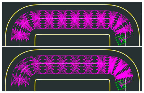
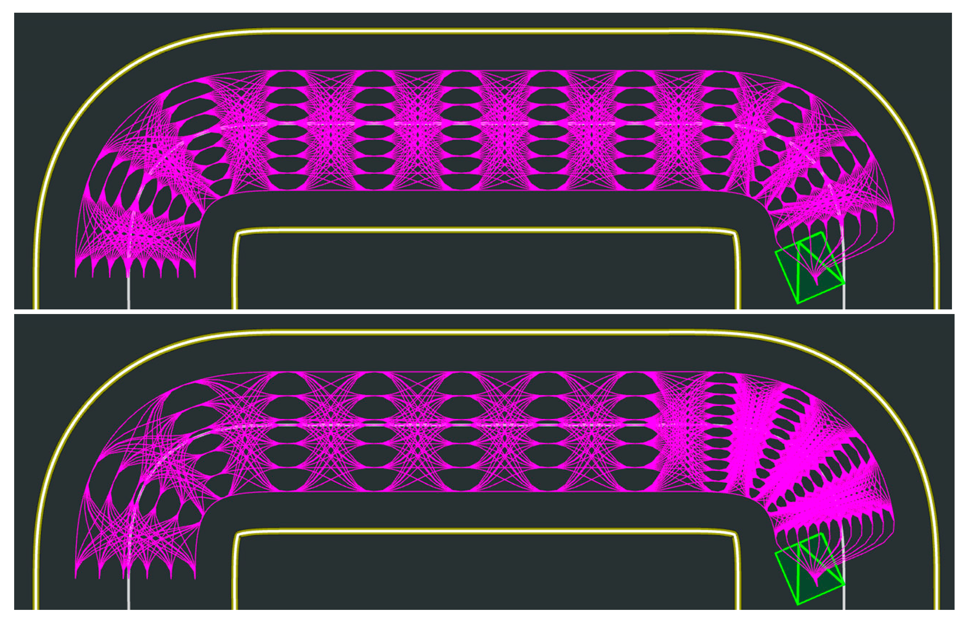
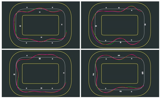
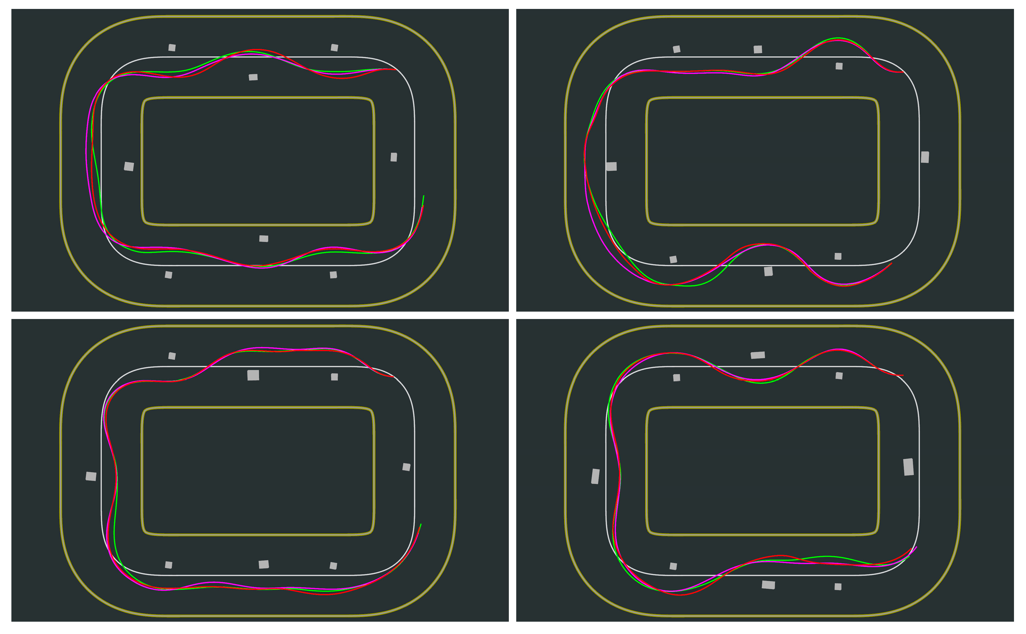
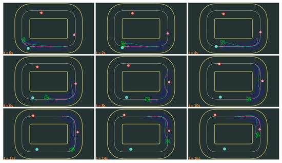
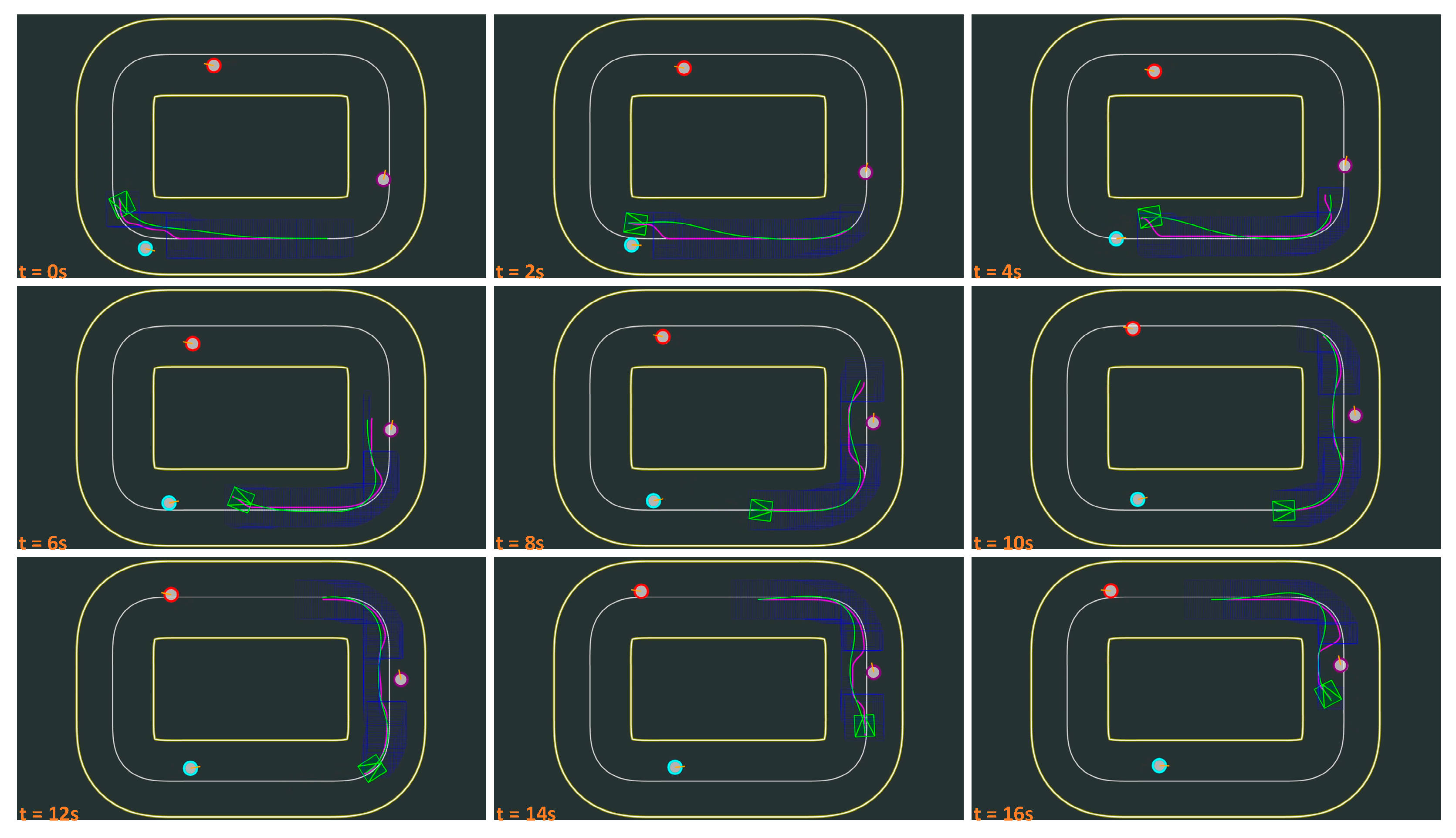
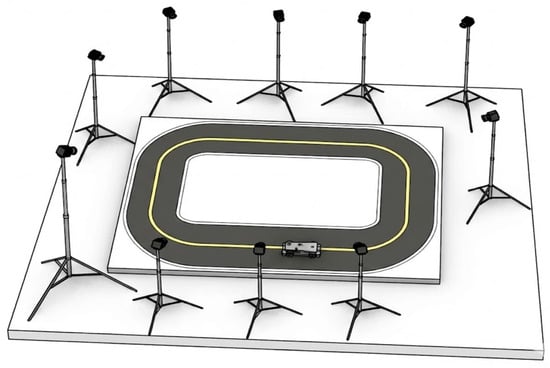
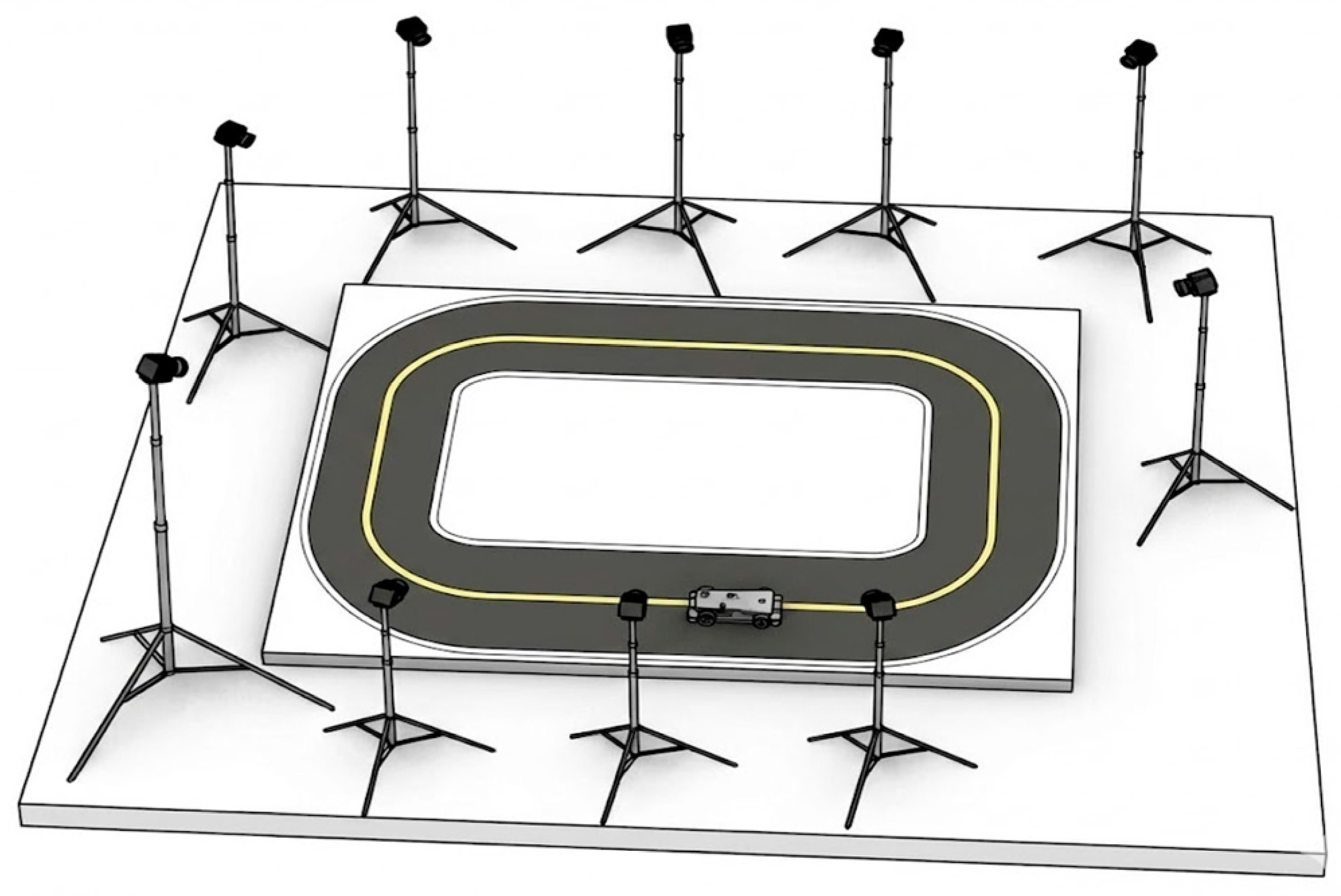
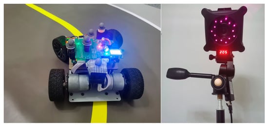
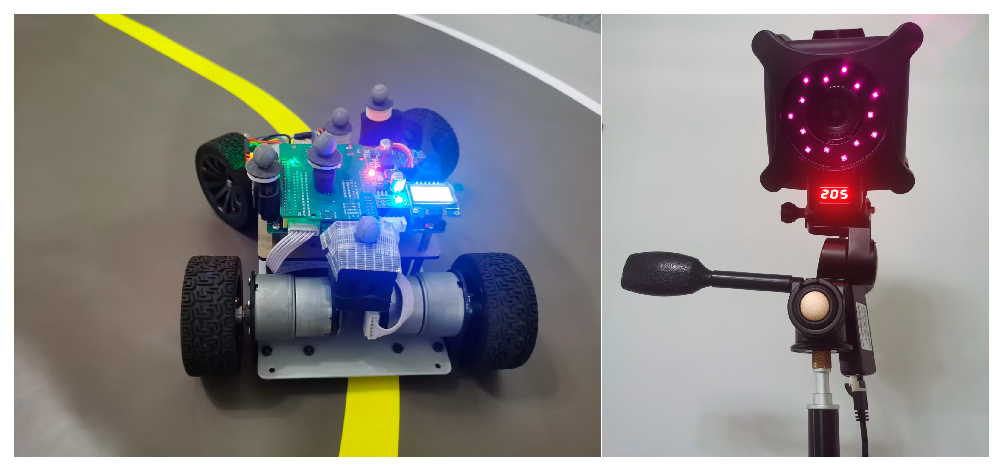
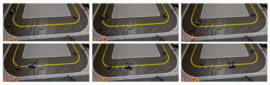
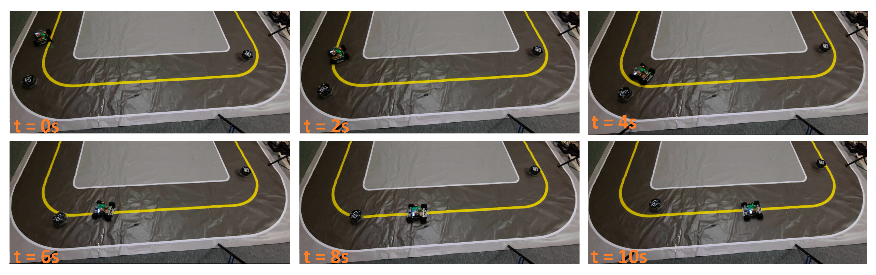
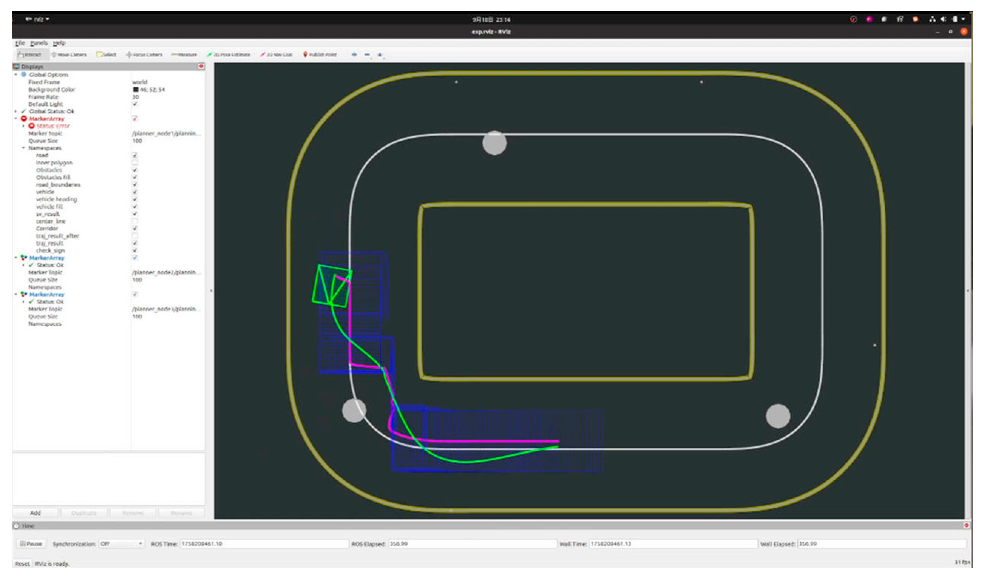

Disclaimer/Publisher’s Note: The statements, opinions and data contained in all publications are solely those of the individual author(s) and contributor(s) and not of MDPI and/or the editor(s). MDPI and/or the editor(s) disclaim responsibility for any injury to people or property resulting from any ideas, methods, instructions or products referred to in the content. |
© 2026 by the authors. Licensee MDPI, Basel, Switzerland. This article is an open access article distributed under the terms and conditions of the Creative Commons Attribution (CC BY) license.