


Abstract
Bridge cranes are essential material-handling equipment, and their main girders must simultaneously satisfy the requirements of lightweight design, stiffness, strength, and fatigue life. Existing optimization studies on crane main girders are mostly based on deterministic methods, whereas the influences of uncertain factors such as plate thickness, material properties, load spectra, and fatigue parameters are rarely quantitatively analyzed. This paper proposes an uncertainty-oriented robust optimization framework for the design of bridge crane main girders. Robustness is rigorously defined as the insensitivity of structural performance to uncertain parameters and is quantified through probabilistic constraints and performance variance indices. A robustness index system comprising static stiffness, dynamic stiffness, static strength, dynamic strength, and fatigue life is established. An improved multi-objective fireworks algorithm (MOIFWA) is adopted, which integrates the explosion search mechanism of the fireworks algorithm with the fast non-dominated sorting and crowding distance strategy of NSGA-II. The cross-sectional dimensions of the main girder are taken as design variables; both mass and deflection are minimized while satisfying constraints on strength, stiffness, stability, and fatigue life. The feasibility of the optimized design is verified through finite element simulations using ANSYS 2022R1, ABAQUS 2025, and FE-Safe 2025. For a 32 t–25.5 m double-girder bridge crane, the optimized main girder achieves a 10.29% reduction in mass and a 5.35% reduction in deflection, with predicted fatigue lives of 34.68 years by the nominal stress/fracture mechanics method and 32.94 years by the ABAQUS/FE-Safe method. This framework provides a practical approach for designing crane girders that are lightweight and possess reliable fatigue performance under uncertainty.
1. Introduction
Bridge cranes are among the most widely used types of lifting equipment in the fields of industrial logistics and mechanical handling. The load-bearing capacity and fatigue resistance of their main girder structures are critical factors determining the operational safety, service reliability, and full life-cycle performance of the entire machine. In current engineering practice, two contradictory tendencies exist in the design of bridge crane main girders, which constrain the optimization of structural performance and the improvement of resource utilization efficiency. On the one hand, to satisfy the lower limits of industry standards, excessive lightweight design is often adopted, while the cumulative fatigue damage caused by load variations and complex service conditions in actual operation is neglected. This practice may readily induce potential safety hazards and shorten the service life of the structure. On the other hand, overly conservative fatigue design based on the upper limits of standards leads to excessive structural redundancy and severe material waste, thereby increasing manufacturing and operating costs and ultimately failing to reconcile structural safety with economic efficiency. Therefore, it is imperative to establish a systematic robustness index system that simultaneously considers static and dynamic stiffness as well as static and dynamic strength, and to conduct optimization research on the influence of uncertain factors such as plate thickness, material properties, load spectra, and fatigue parameters, so as to achieve robust, efficient, and economical optimal design of bridge crane main girder structures.
Methods for structural optimization under uncertainty have advanced from direct worst-case searches to surrogate-assisted and moment-based formulations. Li et al. combined manufacturing tolerances, reliability, and multi-objective evolutionary optimization [1], and Xie et al. used Bayesian estimation to quantify uncertainty in a robust stamping-process design [2]. Rehman and Langelaar reduced the cost of min-max robust optimization through Kriging and adaptive sampling [3]. Dalton et al. considered safety, robustness, and cost in structural design [4], while Cheng et al. developed an interval robust optimization method based on normalized constraint violation and Kriging [5]. Zheng et al. extended robust topology optimization to dynamic structures with hybrid uncertainties [6]. More recent work has approximated stochastic moments non-intrusively [7] or evaluated them analytically by Polynomial Chaos Kriging with active learning [8]. These methods improve uncertainty propagation or reduce model evaluations, but their evidence is drawn mainly from benchmark functions and general structural examples. They do not provide a crane-specific formulation that links cross-sectional variables to spatial deformation, code constraints, random load histories, and fatigue life targets in one optimization model.
Reliability-based design optimization (RBDO) addresses a related limitation of deterministic design by constraining the probability or possibility of failure. Shan and Wang converted the conventional double-loop problem into a reliable-design-space formulation [9], and Strömberg combined second-order reliability analysis with sequential quadratic programming for non-Gaussian variables [10]. Later studies reduced repeated reliability calculations through information reuse in importance sampling [11], adaptive surrogates for interval uncertainty [12], and Kriging-based decoupling [13]. Jerez et al. further considered multiple objectives and stochastic excitation in structural dynamic systems [14]. Although these approaches offer rigorous treatments of uncertainty, they require a credible uncertainty model and repeated limit-state evaluation. In bridge crane design, measured probability distributions are often incomplete, and high-fidelity finite element and fatigue analyses remain expensive. Directly embedding a general RBDO scheme would therefore add computational and data requirements without resolving how crane-specific performance indices should be coordinated.
Existing crane studies provide detailed analyses of individual performance mechanisms. Camber and deformation have been investigated in relation to energy consumption and pre-camber design [15,16]. Digital twin load matching, load spectrum prediction, fracture mechanics, equal-life design, and weld-life extension have improved fatigue assessment [17,18,19,20]. Safety-constrained sizing, response-surface optimization, parametric box girder design, and the joint sizing of ribs and diaphragms have also reduced structural mass or deformation [21,22,23,24]. However, these studies usually optimize nominal dimensions or one class of response. Deformation control is rarely coupled with fatigue damage, and fatigue assessment is commonly performed after a structural scheme has been selected rather than used as an active optimization constraint. As a result, a lighter design can approach an unfavorable fatigue regime, whereas a long-life design can retain unnecessary mass. The literature does not yet explain this tradeoff through a unified set of static, dynamic, stability, and fatigue indices for a bridge crane main girder.
Algorithm selection presents a second unresolved issue. NSGA-II uses fast non-dominated sorting, elitism, and crowding distance to maintain a diverse Pareto set [25]. MOPSO employs an external repository and Pareto-based leaders to guide particle motion [26]. MOEA/D decomposes a multi-objective problem into coordinated scalar subproblems [27], and differential evolution generates trial vectors through scaled population differences [28]. All four methods are established alternatives, but none are uniformly superior across constrained engineering problems: their behavior depends on genetic operators, leader and archive policies, decomposition weights, or mutation and crossover parameters. The present problem has eight continuous sizing variables; competing mass, deflection, and fatigue objectives; and a feasible region restricted by multiple code and service-life constraints. It therefore requires both broad exploration and repeated local refinement near feasible tradeoff solutions.
The multi-objective improved fireworks algorithm (MOIFWA) is selected for this problem because its search mechanisms correspond to those requirements. Fireworks algorithms generate several sparks around each candidate, which supports local sampling of coupled cross-sectional variables [29,30,31]. In MOIFWA, a decreasing explosion radius changes the search from broad exploration to local refinement; Gaussian mutation introduces additional diversity; boundary mapping returns infeasible sparks to the admissible variable range; and NSGA-II non-dominated sorting, crowding distance, and elitist retention control Pareto convergence and spread [25,32,33]. Thus, MOIFWA retains the mature selection mechanism of NSGA-II while replacing conventional crossover and mutation with rank-dependent explosion and mutation searches. The selection is therefore based on the compatibility between the search mechanism and the constrained crane-design problem, rather than being a claim of universal algorithmic superiority.
Accordingly, the research gap is the absence of a bridge crane optimization framework that simultaneously coordinates deformation, static and dynamic stiffness, static and dynamic strength, stability, and fatigue life under practical dimensional constraints, while searching efficiently for multiple engineering tradeoffs. This study addresses that gap in three respects. First, it defines a crane-specific robustness index system that connects spatial deformation and fatigue integrity with the conventional stiffness, strength, and stability checks. Second, it formulates a multi-objective main-girder model in which eight cross-sectional dimensions are optimized to reduce mass and deflection and to bring fatigue life toward the 30-year design target. Third, it develops MOIFWA by combining rank-dependent explosion search and Gaussian mutation with NSGA-II selection, and evaluates the resulting design through ANSYS, ABAQUS, and FE-Safe analyses. The scientific contribution is the coupling of deformation and fatigue within one uncertainty-aware optimization formulation; the practical contribution is a design procedure that can reduce structural redundancy while retaining code compliance and the required service life.
2. Establishment of Robustness Indices for Bridge Cranes
2.1. Composition of Bridge Crane Structure
The bridge crane, commonly referred to as an overhead traveling crane, is a core piece of equipment for three-dimensional heavy-load handling in industrial production. Its stable operation depends on the coordinated functioning of four essential subsystems: the metal structure, the operating mechanisms, the electrical control system, and the safety protection devices. Each subsystem performs distinct functions while providing mutual support to achieve precise load transportation. Specifically, as shown in Figure 1, the hoisting mechanism enables load movement along the vertical axis (Z-axis), the trolley traveling mechanism provides movement along the longitudinal axis (X-axis), and the bridge traveling mechanism realizes movement along the transverse axis (Y-axis) [34].
Figure 1.
Overhead crane.
2.2. Analysis and Construction of Steady-State Indices
2.2.1. Static Stiffness Analysis
1. Vertical Deflection of Main Girder
The vertical deflection of the main girder of a bridge crane is primarily induced by vertical loads, which can be categorized into uniformly distributed loads and concentrated loads. Uniformly distributed loads include the self-weight of the bridge structure, electromechanical equipment, trolley rails, walkways, and railings, all of which are distributed continuously along the main girder. Concentrated loads comprise the lifted load and the self-weight of the hoisting trolley, which are transmitted to the main girder rails through the trolley wheels. As illustrated in Figure 2, the main girder can be idealized as a simply supported beam with one end hinged and the other end on a roller support, subjected to a uniformly distributed load q and concentrated loads P1 and P2 [35,36,37].
Figure 2.
Vertical load of bridge frame structure.
The deflection fCq of the main girder under uniformly distributed load is:
where L—span (mm); x—distance from the trolley to the left end of the span (mm), where x = a1 + c/2; E—elastic modulus of material (N/mm2); and I—section moment of inertia (mm4).
The deflection fCP of the main girder under concentrated load is:
where a—distance from hoisting trolley wheel to the left span end (mm); a1 and a2 correspond to the left and right wheels respectively; b—distance from hoisting trolley wheel to the right span end (mm); b1 and b2 correspond to the left and right wheels respectively; and P1 and P2—wheel loads of hoisting trolley (N).
2. Horizontal Side Sway of Main Girder
Horizontal side sway of the main girder of a bridge crane is primarily induced by horizontal loads, which can be classified into uniformly distributed loads and concentrated loads. During the start-up and braking of the bridge traveling mechanism, the uniformly distributed horizontal load on the main girder arises from the inertial force of the bridge structure itself. The concentrated horizontal load originates from the inertial forces of the hoisting trolley and the lifted load, which are transmitted to the trolley rails through the trolley wheels. As illustrated in Figure 3, the horizontal stiffness of the main girder is evaluated using the frame analysis method, in which the main girder is subjected to a uniformly distributed horizontal load q and concentrated horizontal loads PH1 and PH2 [35,36,37].
Figure 3.
Horizontal load of bridge frame structure.
The horizontal deflection fSq of the main girder under uniformly distributed load is:
where I1—moment of inertia of the main girder section about the vertical y-axis (mm4); I2—moment of inertia of the end carriage section about the vertical y-axis (mm4); ; C—distance from the support on one side of the end carriage to the main girder axis (mm); and B—wheel gauge of the bridge traveling mechanism (mm).
The horizontal deflection fSP of the main girder under concentrated load is:
where PH1 and PH2—horizontal forces of the hoisting trolley wheels (N); φ5—dynamic effect coefficient of the structure under a sudden change in crane traveling driving force; PXC—trolley weight (N); PQ—hoisted load (N); PG—main girder weight (N); a—average traveling acceleration (mm/s2); and g—gravitational acceleration.
2.2.2. Dynamic Stiffness Analysis
1. Vertical Dynamic Stiffness of Main Girder
For bridge-type cranes, when the fully loaded trolley is positioned at the mid-span of the main girder and the load is at its lowest suspended position, the natural frequency in the vertical direction can be determined using an equivalent single-degree-of-freedom vibration system, i.e.,
where me—equivalent mass of the structural vibration system (kg); Ke—equivalent stiffness of the structural vibration system; y0—static displacement of the bridge frame at the load suspension point caused by rated hoisting load (mm); λ0—static displacement (elongation) of the hoisting pulley block under rated hoisting load (mm); β—influence coefficient of structural mass on equivalent mass me; ; m1—converted mass of the structure at the load suspension point (including trolley mass) (kg); and m2—rated hoisting mass (kg).
2. Horizontal Dynamic Stiffness of Main Girder
Horizontal vibration of the bridge crane is primarily induced by the load excitation generated during the start-up and braking operations of the crane traveling mechanisms. The dynamic stiffness in the horizontal direction is
where δe—static displacement of the bridge frame structure under unit horizontal force in the horizontal direction (mm).
2.2.3. Camber Analysis of Main Girder
To reduce the additional energy consumption caused by climbing during trolley travel, camber is preset on the main girder so that the top surface of the main girder remains horizontal at any trolley position, thereby eliminating the climbing resistance of the trolley.
As shown in Figure 4, when the hoisting trolley is located at position x along the main girder, a vertical deflection y is induced in the main girder. To eliminate the gradient resistance caused by this deflection, the actual inclination angle at the corresponding point on the camber curve should be zero, i.e., θ + α = 0, and therefore θ = −α.
Figure 4.
Deflection curve.
The deflection-induced inclination angle of a simply supported beam with a uniform cross-section at position x is given by:
The inclination equation of the deflection curve at any point along the beam is given by:
By integrating the deflection inclination angle equation, the camber curve is obtained as:
When x = 0, the deflection y = 0, in which case C = 0.
Taking the mid-span of the main girder as the coordinate origin and letting x = L/2 − a, the ideal camber curve of the beam under a concentrated load is expressed as:
where fC—maximum deflection of the main girder (mm) and fC = fCq + fCP.
When a = 0, the solution reduces to y1 = fCp/2. It can be observed that the camber at the mid-span of the main girder is equal to half of the deflection induced at the mid-span of the main girder. However, this result accounts only for the deflection caused by concentrated loads, whereas the self-weight of the beam also contributes to the total deflection.
The camber curve of the beam under self-weight load is the negative of the deflection curve induced by the self-weight, expressed as:
The camber curve of the beam under the combined action of concentrated loads and self-weight load is given by:
In addition to the quartic camber curve given in the above equation, commonly used camber curves also include the quadratic parabola, the sine curve, and the three-segment broken line.
Quadratic parabola:
Sine curve:
Three-segment broken line:
where fz—mid-span camber of the main girder (mm), which is generally taken as half of the deflection of the main girder when the fully loaded trolley is located at the mid-span.
Figure 5.
Functional camber curve.
Figure 6.
Three-segment broken-line camber curve.
Figure 5 shows the schematic diagram of the pre-arching in a curve form. M(x, y) represents the various curve forms corresponding to the pre-arching of the main beam.
2.3. Structural Life Analysis and Research
2.3.1. Static Strength
The static strength check of the main girder shall be performed at the critical section under the most unfavorable load combination to determine whether the design service requirements are satisfied. For a main girder with a biased rail configuration, the critical stress points can be classified into four types, as illustrated in Figure 7: (1) the joint between the main web and the upper flange plate; (2) the joint between the secondary web and the bulkhead; (3) the joint between the secondary web and the lower flange plate; and (4) the edge of the lower flange plate [37].
Figure 7.
Critical calculation points of main girder section.
1. Bending Stress
1) Vertical Direction
When the concentrated load from the hoisting trolley wheels is transmitted to the main girder through the wheel pressure, the maximum bending moment is given by:
The maximum shear force in the main girder occurs when the trolley is positioned at the beam end.
2) Horizontal Direction
When the main girder is modeled as a frame in the horizontal plane, the mid-span bending moment induced by concentrated and uniformly distributed loads is given by:
The maximum stress at the corner point of the flange plate at the mid-span section is given by:
where Mx—the sum of bending moments induced by vertical concentrated loads and uniformly distributed loads on the calculated section (N·mm); Wx and Wy—the section flexural moduli of the calculated section in vertical and horizontal directions, respectively (mm3).
The maximum shear stress in the web at the beam-end section is given by:
where Q—the shear force of the calculated section (N); Sx—the maximum static moment of the section at the shear stress location (mm3); and δ is the web thickness (mm).
2. Constrained Bending Stress
where σWP and σWq—the free bending stresses (N) induced by concentrated load and uniformly distributed load; φP and φq—the overstress coefficients of restrained bending at the mid-span section of the beam under concentrated load and uniformly distributed load.
3. Restrained Torsion Stress
Biased rail box girders and slightly biased rail box girders are subjected to torque under the combined action of trolley wheel pressure and horizontal forces, resulting in torsional deformation of the main girder. The total torque Mn is the sum of the vertical torque component MnV and the horizontal torque component MnH, i.e., Mn = MnV + MnH.
The bending moment induced by the vertical load is given by:
where φi and φj—the dynamic load factors, determined according to load combinations; e—the distance from the bending center of the main girder section to the rail centerline (mm).
The bending moment induced by the horizontal load is given by:
where h—the height of the main girder (mm); hg—the height of the trolley rail (mm); and h2—the distance from the trolley center of gravity to the top surface of the trolley rail (mm).
4. Average Bearing Stress on Main Web Induced by Trolley Wheel Pressure
For a biased rail box girder, the trolley rail is positioned above the main web. The average bearing stress in the main web induced by the trolley wheel pressure is given by:
where P—the wheel pressure of a single wheel (N); δ1—the thickness of the main web (mm); and hy—the sum of trolley rail height and upper flange plate thickness (mm).
5. Resultant Stress
The resultant stress, which accounts for both the restrained torsional normal stress and the restrained bending normal stress, is given by:
The resultant shear stress is given by:
At the junction between the upper flange plate and the main web at the mid-span section of the biased rail box girder, compressive stress exists in addition to normal stress, and the composite stress is given by:
Composite Stress at the Junction between the Lower Flange Plate and the Main Web
2.3.2. Dynamic Strength Analysis
The fatigue strength of the main girder depends on the working stress spectrum, the number of stress cycles, the joint type reflecting stress concentration, the stress cycle characteristics, and the maximum stress at the fatigue-critical locations.
Allowable tensile fatigue stress of weld:
2.3.3. Fatigue Strength Life Analysis
In the manufacturing of crane bridge structures, conventional welding processes may fail to meet the service requirements. With the rapid advancement in science and technology, the probability of initial cracks arising during welding has been significantly reduced. Therefore, the nominal stress–fracture mechanics method is adopted for fatigue life analysis.
1. Nominal Stress Method
The nominal stress method is an approach for evaluating crack initiation life based on the S–N curve. It is applicable to components without cracks or defects. The basic fatigue curve is obtained by applying symmetric cyclic stress with a stress ratio of R = −1 to standard specimens.
When expressed in logarithmic coordinates, stress (S) and life (N) exhibit a linear relationship.
where m, C, A and B—material constants. m and C are related to factors such as stress ratio and loading mode, while A = lgC/m and B = −1/m.
When R = −1, the fatigue limit under rotating bending load can be estimated as:
Under rotating bending loads, the fatigue limit Sf of different materials typically ranges from 0.3 to 0.6 times the ultimate tensile strength Su.
When estimating the S-N curve in the absence of experimental data:
For bending, k is taken as 0.5; for compression, k is taken as 0.35; and for torsion, k is taken as 0.29.
In terms of the S-N curve, C = (k Su)m × 103, and the calculation method of parameters C and m that can be deduced from the above curve expression is: m = 3/lg (0.9/k) and C = 0.9 (0.9Su)m × 103.
2. Fracture Mechanics Method
Fracture mechanics primarily investigates the propagation behavior of macroscopic cracks in materials and engineering structures. Its core aspects include the conditions for crack initiation, the crack growth process under external loads, and the critical fracture state. In addition, it encompasses the assessment of failure conditions for cracked structures, the determination of safe crack sizes, and the prediction of residual life [19].
Figure 8.
da/dN-ΔK curve.
The fatigue crack growth rate, da/dN (or da/dt), refers to the rate of change in crack length a with respect to the number of cycles N (or loading time t) under fatigue loading, reflecting the speed of crack propagation. The stress intensity factor range, ΔK, is an important parameter characterizing fatigue crack growth, representing the range of the stress intensity factor that drives crack propagation.
Region I: Low-rate region. In this region, the crack growth rate is relatively low. When the stress intensity factor range is below the threshold value, the crack is considered to be non-propagating.
Region II: Intermediate-rate crack growth region (stable crack growth region). In this region, the curve is approximately linear, and the crack growth rate typically ranges from 10−9 to 10−5 m/cycle. The linear relationship between lg(da/dN) and lg(ΔK) can be expressed as:
Region III: High-rate region. In this region, the crack growth rate increases rapidly, corresponding to the unstable crack propagation zone.
3. Engineering Case of Robustness Analysis
3.1. Design Case Parameters
A 32 t–25.5 m double-girder overhead crane is selected as the research object. The specific parameters are shown in Table 1.
Table 1.
Parameters of 32t−25.5m A6 double-girder overhead crane.
The cross-section of the main girder is shown in Figure 9.
Figure 9.
Main girder section.
The cross-sectional parameters of the main girder are listed in Table 2.
Table 2.
Sectional dimension parameters of main girder.
3.2. Spatial Deformation Analysis
The aforementioned formulas are employed to calculate the theoretical deflections, including vertical deflection and horizontal side bending, of the crane under different loading conditions. The calculation results are presented in Table 3 and Table 4.
Table 3.
Theoretical calculation results of under-camber for overhead crane main girder.
Table 4.
Theoretical calculation results of lateral bending for overhead crane main girder without pre-camber.
As shown in Table 3 and Table 4, the overhead crane exhibits relatively large deformation in the vertical direction and small deformation in the horizontal direction. This can be attributed to the fact that the vertical direction sustains a greater load, including the dead weight of the entire crane and the hoisted load. The hoisted load is large and highly concentrated, resulting in substantial deformation. In contrast, the horizontal load is relatively small and mainly originates from the inertial forces generated during the starting and braking of the crane traveling mechanisms. Compared with the allowable vertical deflection [f] = L/1000 = 25.5 mm and the allowable horizontal deflection [f] = L/2000 = 12.75 mm specified in the standard, both deformations satisfy the stiffness requirements.
3.3. Fatigue Life Analysis
1. Acquisition and Data Processing of Stress Spectrum for Overhead Crane
1) Load Spectrum of Overhead Crane
Based on the actual operating data of the crane measured over a period of one month at the site, the existing load spectrum of the bridge crane was plotted (as shown in Figure 10). Random simulations of the crane’s working cycle were conducted to reproduce its operating conditions in the actual scenario. Subsequently, the finite element model of the cantilever crane was established and analyzed using finite element software. Through numerical calculations, the stress history curves of each critical stress point during the crane’s operation were obtained.
Figure 10.
Load spectrum.
For the existing load spectrum data, parameter fitting is required to convert the discrete data into a mathematical distribution function, thereby facilitating the subsequent fatigue life calculation and cross-section optimization of the main girder of the overhead crane. In this paper, the Weibull–Gamma distribution function, which exhibits favorable approximation performance, is selected for parameter fitting.
Weibull–Gamma mixture model function:
where ω denotes the weight; A is the amplitude factor; k is the shape parameter of the Weibull function; λ is the scale parameter of the Weibull function; α is the shape parameter of the Gamma function; β is the scale parameter of the Gamma function; and Г() is the Gamma function.
The code for the Weibull–Gamma mixture function is implemented in MATLAB R2022b. Multiple iterations are performed by substituting different shape and scale parameters of the Weibull and Gamma distributions to obtain the fitting curve that best matches the load spectrum. Meanwhile, it is observed that the individual fitting errors of the Weibull function and the Gamma function are relatively large. Therefore, the Weibull–Gamma mixture function is adopted. The fitted parameter results are illustrated in Figure 11.
Figure 11.
Comparison of curve fitting performance for the Weibull, Gamma, and Weibull–Gamma mixture models.
As shown in Figure 11, Figure 12 and Figure 13, the residual scatter plots indicate that the single Weibull and Gamma distribution models exhibit significant systematic bias. Among them, the Gamma model has the largest RMSE (0.0032), whereas the Weibull–Gamma mixture model yields an RMSE of only 0.0014, with residuals concentrated around the zero baseline, indicating a marked reduction in systematic error. Comparison of the fitted curves reveals that the single-distribution models deviate noticeably from the measured scatter points in the low-load range, at the peak, and in the load tail, whereas the Weibull–Gamma mixture model closely fits the original data, with an R2 as high as 0.9841, outperforming the Weibull (R2 = 0.9481) and Gamma (R2 = 0.9170) models. Furthermore, the bar chart of multiple evaluation metrics confirms that the Weibull–Gamma mixture model achieves the highest R2 and adjusted R2, the smallest RMSE and MAE, and the lowest AIC and BIC values, demonstrating the best overall performance. In summary, the single Weibull and Gamma distributions are insufficient to accurately describe the hoisting load distribution, whereas the Weibull–Gamma mixture distribution provides a superior fit and can offer reliable support for subsequent load spectrum derivation and structural fatigue life assessment.
Figure 12.
Parameter fitting curve distribution of Weibull–Gamma hybrid model function.
Figure 13.
Comparison of multiple evaluation metrics for the Weibull, Gamma, and Weibull–Gamma mixture models.
2) Acquisition of Stress History Curves
To obtain realistic stress history curves, it is necessary to randomly simulate the travel path of the trolley and acquire the stress–time curve at a specific node of the main girder within a given period. By simulating multiple curves under different paths, the stress history curve corresponding to a particular path can be obtained. This process is defined as one working cycle, and the travel paths adopted in the simulation are shown in Figure 14 and Table 5.
Figure 14.
Trolley position diagram.
Table 5.
Trolley running simulation path.
The transient dynamics module in the finite element software is employed to calculate the stress cycles at critical points on the cross-section of the main girder. The displacement of the trolley is applied using a function-driven method, and the loads are imposed on the upper surface of the trolley frame. The travel trajectory of the trolley is simulated, and the stress variation curve at a specific point of the main girder within one working cycle is extracted, as shown in Figure 15.
Figure 15.
Stress–time diagram.
By simulating the traveling path of the trolley, the stress history curves of four critical stress points on the mid-span cross-section of the main girder are calculated and plotted as shown in Figure 13, which reflect the stress histories of the calculation points during a certain operating period of the crane. Afterwards, repeated working simulations are performed for the trolley moving from one position to another, and the stress history curves of the four critical points on the main girder cross-section are computed and integrated into 60 sets of traveling path curves. The simulation data are processed to obtain the stress history curves of the four calculation points presented in Figure 16.
Figure 16.
Stress history curve.
3) Rainflow Counting Method
The obtained stress history curves at each critical stress calculation point are complex and cannot be directly employed in subsequent calculations. Simplification is therefore required to decompose the complicated stress histories into individual stress cycles. The most widely adopted method for this purpose is the rainflow counting method, as illustrated in Figure 17.
Figure 17.
Rainflow counting method overview diagram.
The partial data processing results are shown by the red line in Figure 18.
Figure 18.
Data processing of the rainflow technology section.
4) Stress Amplitude Correction
In this study, both the nominal stress method and the fracture mechanics method are adopted for fatigue life calculation. The nominal stress method is applied using symmetric cycles with a stress ratio of R = −1, whereas the fracture mechanics method employs the Paris equation with pulsating cycles characterized by a stress ratio of R = 0.
The data processed by the rainflow counting method cannot be directly used for fatigue life evaluation via the nominal stress method or the fracture mechanics method. Therefore, stress amplitude correction is required to convert the rainflow-counted data into symmetric cycles with a stress ratio of R = −1. The specific correction formula is given as follows:
where σa−1—the stress amplitude under R = −1 (MPa); σa—the stress amplitude extracted by the rainflow counting method (MPa); σm—the mean cyclic stress (MPa); and σb—the tensile strength of the material (MPa).
The corrected stress cycles (as shown in Figure 19) are symmetric cycles, which are suitable for the calculation of crack initiation life. Since the Paris equation is adopted for crack propagation life calculation, further correction to pulsating cycles with a stress ratio of R = 0 (as shown in Figure 20) is required, as expressed in Equations (43) and (44):
where σa0 denotes the stress amplitude under R = 0 (MPa).
Figure 19.
Stress amplitude correction for R = −1.
Figure 20.
Stress amplitude correction for R = 0.
5) Determination of Key Parameters for Fatigue Crack Propagation Life Evaluation
(1) Initial Crack Size a0
The initial crack size a0 refers to the initial crack dimension adopted in the calculation of crack propagation life. According to existing inspection data, the initial crack size generally ranges from 0.05 to 0.5 mm [38].
(2) Critical Crack Size ac
The critical crack size ac is the maximum crack size at which brittle fracture will not occur when the material is subjected to external forces or loads. In calculations, it is generally determined by the maximum stress intensity factor for stable crack growth or the minimum stress intensity factor for unstable crack propagation, and its calculation is expressed as follows:
where KIC—the fracture toughness of the material (N/mm3/2); α—the shape factor; and σ—the maximum cyclic stress (MPa).
(3) Shape Correction Factor YS
The shape correction factor is generally a function of the crack size a and the plate width W. For the main girder structure of bridge cranes, YS = 1.12 [39].
(4) Fracture Toughness KC
Fracture toughness is a material property that represents the material’s capacity to resist crack propagation. For Q235 steel used in bridge cranes, the fracture toughness is taken as KC = 191.4 MPa [39].
(5) Fatigue Crack Growth Rate Parameters C and m
The parameters C and m in the Paris equation follow a normal distribution with a mean value of 3 and a standard deviation of 0.03. Based on box girder tests carried out at Taiyuan University of Science and Technology, a set of values was obtained: C = 2.606 × 10⁻¹⁰ and m = 2.965 [39].
2. Crack Initiation Life of Bridge Crane Based on Nominal Stress Method
The nominal stress method is employed to calculate the maximum crack initiation life that can be obtained by this method. It describes the process whereby, under continuous alternating loads and in the absence of initial defects, the material undergoes progressive degradation and cracks eventually emerge after high-cycle stress cycling.
Q235 steel is selected as the crane material in this study. According to the loading characteristics of the crane main girder, a correction factor of k = 0.35 is adopted. The constants C and m in the S–N curve are subsequently determined. Based on the computed stress history curves under symmetric cycles, Equation (46) is applied to calculate the crack initiation life Nm:
3. Crack Propagation Life of Bridge Crane Based on Fracture Mechanics Method
The Paris equation is adopted for the calculation of crack propagation life. By integration, the fatigue crack propagation life NP can be expressed as:
If the shape factor a is independent of crack size a,
- when m ≠ 2
Total Fatigue Life
The nominal stress method is used to calculate the fatigue life from the state of no initial cracks to the generation of initial cracks. The Paris formula, on the other hand, is used to analyze and calculate the crack propagation life under the condition of an initial crack size. In summary, the total fatigue life of the crane main girder structure consists of the crack initiation life and the crack propagation life induced by load actions. The total structural life is calculated by superposing these two components, as expressed below:
where N—the total fatigue life of the structure (year); G—the annual working cycles of the structure (times).
As shown by the fatigue life results for each calculation point in Table 6, the service life of the crane main girder structure during the crack initiation stage is relatively long. The position where fatigue fracture first occurs on the main girder is generally identified as Calculation Point 3 (the connection between the secondary web and the lower flange plate), where the shortest service life is 52 years.
Table 6.
Total fatigue life at each calculation point.
4. Robust Structural Optimization
4.1. Robust Optimization Process
In Section 2, the robustness indicators of the selected bridge crane were analyzed. The results demonstrate that its strength, stiffness, and fatigue life satisfy the design service requirements, while a certain design margin still remains. Specifically, the fatigue life of the main girder structure is 52 years, which considerably exceeds the design service life of 30 years. Therefore, the multi-objective fireworks algorithm is introduced to optimize the crane main girder. The optimization aims to adjust the fatigue life to a reasonable range while satisfying the design service requirements of the main girder. The specific robust optimization process is shown in Figure 21.
Figure 21.
Robust optimization flowchart.
4.2. Multi-Objective Fireworks Algorithm
4.2.1. Overview of the Multi-Objective Fireworks Algorithm
The core idea of the multi-objective improved fireworks algorithm (MOIFWA) is to combine the explosion search mechanism of the fireworks algorithm (FWA) with the fast non-dominated sorting strategy of NSGA-II. Its basic procedure is as follows: in each generation, each “firework” (i.e., a candidate solution) generates a varying number of “sparks” (i.e., new solutions) according to its quality, represented by its non-dominated rank, so as to perform local search. Subsequently, the population composed of fireworks and sparks undergoes fast non-dominated sorting and crowding distance calculation within the NSGA-II framework, thereby selecting the next-generation population and guiding the search toward the Pareto front. In this study, different parameter perturbations, namely the plate thickness dimensions of the main girder, random loads, and fatigue life parameters, are imposed on the algorithm to transform it into a robust multi-objective fireworks algorithm.
4.2.2. Optimization Model
The objective functions are established with the optimization goals of minimizing the main girder weight and minimizing the deflection.
1. Definition of Dominance Relation
1) Definition of Dominance Relation
Feasible solutions dominate infeasible solutions: V(xi) = 0 and V(xj) > 0.
Lower constraint violation dominates higher constraint violation: V(xi) > 0, V(xj) > 0, and V(xi) < V(xj).
Pareto dominance between feasible solutions holds if and only if:
where the constraint violation V(xi) is defined as
In this equation, the first term represents the normalized violation of the deterministic constraints, and the second term is the penalty term for insufficient reliability, where λ is a large penalty coefficient.
The reliability R(xi) is defined as R(xi) = minjRj(xi), where Rj(xi) denotes the sampling-estimated reliability of the -th probabilistic constraint.
2) Non-dominated Sorting Algorithm
The current population is subjected to non-dominated sorting, and individuals are divided into multiple Pareto front ranks (Front1, Front2, …).
2. Crowding Distance Calculation
Within each non-dominated layer, the crowding distance of individuals is calculated to characterize the distribution of solutions in the objective space. Individuals with larger crowding distances are preferentially retained to prevent excessive aggregation of the solution set. The crowding distance D is calculated as follows:
where fmmax and fmmin—the maximum and minimum values of objective m in the current front.
For boundary solutions, Di is set to ∞. Since itself is a robust objective, Di reflects the distribution density in the robust objective space rather than that in the deterministic objective space.
To further enhance robustness, this study introduces a reliability-weighted term into the standard crowding distance:
where η ≥ 0 denotes the reliability weight.
This modification enables solutions with higher reliability to obtain a larger crowding distance under the same distribution density. Near the Pareto front boundary, solutions with insufficient reliability are downweighted even if their objective values are close.
3. Explosion Operation
1) Explosion Radius
The explosion radius in the multi-objective fireworks algorithm differs from that in the traditional single-objective fireworks algorithm. To achieve better iterative performance, a large-scale search is adopted at the initial stage of the algorithm. As the iteration proceeds, the optimal solution needs to be searched within a progressively reduced range. For this purpose, a gradually decreasing sequence is selected to calculate the explosion radius. The calculation formula for the explosion radius Ai is given as follows:
2) Mutation Sparks
New explosion sparks and Gaussian mutation sparks are generated through the explosion operation. For each dimension k, the new spark is expressed as:
To enhance diversity, a portion of the sparks generated by the explosion are selected for Gaussian mutation. The Gaussian mutation spark is expressed as:
where N(0,1) is a random number following the Gaussian distribution, and γ denotes the mutation coefficient with random iterative attenuation.
3) Quantity of Explosion Sparks
where ri—the front rank of the spark; α and β—adjustment parameters.
During the firework explosion operation, the generated sparks may exceed the boundaries of the feasible region. Therefore, sparks outside the feasible region are mapped back into the feasible region using mapping rules, and the number of sparks produced by each firework is restricted.
4. Elitist Preservation Strategy
Similar to the elitist selection strategy of fast non-dominated sorting, the parent population and the offspring population are combined. Subsequently, the merged population is sorted according to indicators such as crowding distance and Pareto rank for individual retention. The crowding distance of individual xi is expressed as:
4.3. Robust Optimization Model
In this study, robustness is defined as the insensitivity of structural performance to the specified uncertainty vector while maintaining the required probability of constraint satisfaction. For objective j, performance stability is quantified by the robust measure Rj(x) = μj(x) + κjσj(x), where μj and σj are the sample mean and standard deviation and κj is the robustness penalty coefficient. Constraint robustness is quantified by the chance constraint P[g(x,ξ) ≤ 0] ≥ 0.90. The uncertainty vector ξ contains dimensional deviations, the random hoisting load, material-property variation, and fatigue parameters. Accordingly, a design is considered robust only when it combines low response dispersion with the prescribed reliability; robustness is not inferred from the nominal optimum alone.
4.3.1. Establishment of Robust Constraint Indices
1. Deterministic Robust Constraint Indices
1) Static Stiffness
2) Dynamic Stiffness
3) Static Strength
4) Dynamic Strength
5) Global Stability
6) Local Stability
2. Uncertain Robust Constraint Indices
In this study, robustness is defined as the ability of a design to maintain acceptable structural performance and to satisfy the prescribed probabilistic constraints under the specified uncertainty vector. In robust optimization, in addition to the hoisting load PQ, the manufacturing tolerances of the main girder plate thicknesses and the randomness of initial weld crack sizes also influence structural stiffness, stress distribution, and fatigue life. These three types of parameters are treated as uncertain parameters and incorporated into the robustness evaluation; together with the hoisting load, they constitute the uncertain parameter vector.
1) Plate Thickness Dimensions
(1) Plate Thickness Variation
During the manufacturing of steel structural components, the actual thickness of each plate is influenced by the rolling process, shearing precision, and welding deformation, and consequently fluctuates around the design nominal value. For steel plates used in cranes, the minimum thickness is 6 mm, and even values are generally adopted. According to GB/T 709, the plate thickness tolerance is generally controlled within ±3% to ±5% of the nominal thickness.
For the i-th plate thickness dimension, the nominal value is xinom, and the actual plate thickness is expressed as:
where εi is the relative deviation, which is assumed to follow a normal distribution:
where COVi2 denotes the coefficient of variation, which is determined according to the manufacturing tolerance.
(2) Sampling Method
For the plate thickness tolerance, stratified inverse transform sampling is adopted. The range [0, 1] of the standard normal cumulative distribution function is equally divided into Ns subintervals. Within each subinterval, a uniform random number uk is generated, and the inverse transformation is then applied to obtain:
Consequently, a sample set of plate thicknesses is obtained. The plate thickness tolerance affects the deflection, stress, and fatigue life by altering the cross-sectional moment of inertia, section modulus, and mass of the main girder.
2) Random Loads
Among the service loads acting on the main girder of a bridge crane, the hoisting load varies with the operating task and exhibits the largest fluctuation, making it the most significant uncertain factor affecting the deflection, stress, and fatigue life of the main girder. In this study, the trolley self-weight, uniformly distributed load, dynamic load factor, and horizontal inertial load are taken as their design nominal values, and only the hoisting load PQ is treated as a random variable. The hoisting load is fitted using aWeibull–Gamma mixture model based on the measured load spectrum. Stratified inverse transform sampling is adopted: the range [0, 1] of the cumulative distribution function is first equally divided into non-overlapping subintervals, and a uniform random number is generated within each subinterval. Subsequently, samples of the hoisting load are obtained by solving FPQ(PQ,k) = uk using a numerical root-finding method. Ns is set to 1000–5000, and the convergence criterion is that the relative deviations of the mean and standard deviation do not exceed 1% and 3%, respectively.
(1) Distribution Model of the Hoisting Load
The hoisting load PQ follows a Weibull–Gamma mixture distribution, and its cumulative distribution function is given by:
The corresponding cumulative distribution function is given by:
(2) Stratified Sampling and Inverse Transformation
The hoisting load is a univariate random load, and the sampling process is divided into two stages: first, stratified uniform random numbers are generated over the range of its cumulative distribution function, then inverse transformation is performed to obtain hoisting load samples that follow the Weibull–Gamma mixture distribution.
First stage: Stratified uniform sampling
The range [0,1] of FPQ is equally divided into Ns non-overlapping subintervals:
Within each subinterval, a uniform random number is independently generated as follows:
where rk denotes the uniform perturbation term within the k-th subinterval, which is used to avoid sample points being fixed at the midpoint of each subinterval. Compared with pure random sampling, stratified sampling ensures that exactly one sample is generated within each subinterval, thereby yielding more stable statistical estimates with a smaller sample size.
Second stage: Inverse transformation mapping
Since FPQ(x) has no explicit analytical inverse function, a numerical root-finding method is adopted to solve:
The bisection method is employed to iteratively solve the equation within the interval [0, PQ,max] with the convergence tolerance set to 10−6, thereby yielding the hoisting load samples:
Consequently, a sample set of hoisting loads is obtained {PQ,1, PQ,2, …, PQ,Ns}.
Its distribution approximates the original Weibull–Gamma mixture distribution and exhibits stratified uniformity in the probability space, thereby avoiding the insufficient sampling in the high-load tail region associated with pure random sampling.
(3) Sampling Size and Convergence
The sample size Ns directly affects the accuracy of the robust objective and reliability estimation. To verify the sampling convergence, the mid-span deflection fC of the main girder is taken as an example, and the variations in its mean and standard deviation with Ns are monitored:
When the sample size is increased from Ns to 2Ns, if the following condition is satisfied:
the sampling is considered to have converged. Otherwise, is further increased until the convergence criterion is met.
3) Initial Crack Size
(1) Initial Crack Size Variation
The initial crack size of welded structures depends on the welding process, material metallurgical quality, non-destructive testing (NDT) capability, and acceptance criteria. According to BS 7910, IIW recommended practices, and existing inspection data, the initial crack size generally ranges from 0.05 to 0.5 mm, and its distribution is markedly right-skewed—most components have small initial defects, while a few components contain relatively large initial cracks. Therefore, is assumed to follow a lognormal distribution:
The probability density function of is given by:
The mean initial crack size is taken as μao = 0.1 mm, and the coefficient of variation is taken as COVa0 = 0.5, yielding σlna = √ln(1 + COV2) ≈ 0.47 and μlna = lnμa0 − 0.5 × σ2lna ≈ −2.41. This lognormal distribution ensures that remains strictly positive, and its upper tail covers the inspection upper limit of 0.5 mm.
(2) Sampling Method
Stratified inverse transform sampling is adopted. The interval [0, 1] is equally divided into Ns subintervals, and a uniform random number uk is generated within each subinterval. Through inverse transformation, the following is obtained:
4) Uncertainty in Combined Parameters
The hoisting load, plate thickness tolerance, and initial crack size are combined into an uncertain parameter vector, expressed as:
Stratified inverse transform sampling is performed separately for each uncertain parameter, yielding sets of samples: {ξ1, ξ2, …, ξNs}. Specifically, the hoisting load is sampled using the numerical root-finding inverse transformation of the Weibull–Gamma mixture distribution; the plate thicknesses and cross-sectional dimensions are sampled using normal inverse transformation; and the initial crack size is sampled using lognormal inverse transformation. To eliminate artificial correlations among variables, the stratified ordering of each variable is randomly permuted, so that the sample matrix is uniformly distributed in the probability space.
For the j-th performance objective , the robust objective is defined as:
where μfj(x) and σfj(x) are the sample mean and standard deviation of fj(x, ξ), respectively, and kj ≥ 0 is the robustness penalty coefficient. A larger kj places greater emphasis on reducing performance dispersion. Thus, the robust objective simultaneously considers nominal performance and insensitivity to uncertainty.
For the k-th constraint gk(x, ξ) ≤ 0, constraint robustness is quantified by the chance constraint
where Rkmin is the minimum acceptable reliability. In this study, Rkmin = 0.90 is adopted as the minimum requirement, and stricter values can be used if required by codes or project specifications.
The sample mean, standard deviation, and reliability are estimated by stratified inverse transform sampling:
where NS is the sample size and I[ ] is the indicator function. The sampling convergence is checked by requiring the relative changes in the mean and standard deviation to be less than 1% and 3%, respectively.
Accordingly, a design is considered robust only when it simultaneously exhibits low response dispersion and satisfies the prescribed reliability. Robustness is therefore not inferred from the nominal optimum alone; it is quantified through the coupling of μfj(x), σfj(x), and P[gk(x,ξ) ≤ 0].
4.3.2. Design Variables
Structural optimization of the main girder is carried out by adjusting the cross-sectional dimensions. Under the premise of satisfying the strength, stiffness, and stability requirements of the bridge structure, the weight of the main girder is reduced as much as possible while optimizing the service life of the bridge crane. Therefore, structural optimization aims to search for a set of optimal cross-sectional dimensions.
where x1, x2, x3, x4, x5, x6, x7, and x8 represent the width of the upper flange plate, thickness of the upper flange plate, width of the lower flange plate, thickness of the lower flange plate, web height, thickness of the main web, thickness of the secondary web, and web spacing (mm), respectively. Considering the feasibility in practical manufacturing, the plate thickness and plate width are generally integers.
4.3.3. Objective Function
With the length and material density of the main girder held constant, the optimization objective is to minimize the volume and weight of the main girder, minimize the deflection, and bring the fatigue life as close as possible to the target service life of 30 years (i.e., minimize the deviation between the calculated fatigue life and the design service life).
The function expressions are as follows:
Weight:
where 1.2 is the coefficient accounting for the weight of the internal diaphragms and other components of the main girder.
Deflection:
The design variables are selected as the plate thickness, length, and width. Considering the deviations arising from the manufacturing process, the actual structural dimensions are expressed as xact = x + Δx. The uncertainty vector ξ includes the plate thickness deviation, the actual hoisting load PQ, and the initial crack size a0, which induce fluctuations in the objective functions. The robustness objective functions are formulated as follows:
The weight robustness objective function is given by:
The vertical deformation robustness objective function is given by:
Robust fatigue life objective:
4.3.4. Constraint Conditions
The optimization constraints for the main girder structure mainly include two categories: dimensional constraints and structural design indices.
Constraint conditions are established for the optimization model, as shown in Table 7.
Table 7.
Types and expressions of constraint conditions.
4.4. Algorithm Comparison
To quantitatively compare the performance of the proposed MOIFWA against NSGA-II, MOPSO, MOEA/D and standard FWA for robust multi-objective optimization of the bridge crane main girder, the 3D Pareto distribution and four standard multi-objective metrics (HV, IGD, spacing and spread) are shown in Figure 22a–e. Figure 22a displays Pareto-optimal solutions in the objective space of mass robustness, deflection robustness and fatigue life robustness. The non-dominated solutions from MOIFWA span a wider Pareto front and reach regions with lower mass and deflection while maintaining good fatigue life, showing stronger exploration capacity than the other four algorithms.
Figure 22.
Performance comparison of the five algorithms: (a) three-dimensional Pareto front comparison; (b) HV convergence curve; (c) IGD convergence curve; (d) spacing convergence curve; (e) spread convergence curve.
Figure 22b gives the HV convergence curves. MOIFWA achieves the fastest HV rise in early generations and keeps the highest HV throughout the optimization, peaking at the 60th generation. A higher HV represents better convergence and front coverage, proving that MOIFWA can rapidly obtain high-quality non-dominated sets. Figure 22c shows IGD convergence trends. MOIFWA’s IGD falls much faster than its rivals and converges to the lowest steady value; a smaller IGD means that solutions lie closer to the true Pareto frontier, confirming its superior convergence accuracy.
Figure 22d plots spacing curves measuring the uniformity of solutions on the Pareto front. While all algorithms experience obvious spacing fluctuations in the first 10 generations, MOIFWA stabilizes at the minimal spacing after around 20 generations, indicating more evenly distributed Pareto points. Figure 22e presents the spread metric that describes the overall range of the solution set. MOIFWA has high spread at the initial search stage, indicating strong global exploration. Its spread gradually decreases and stabilizes at the lowest level in later iterations, showing effective balance between exploration and exploitation to avoid excessive solution dispersion. Overall, the Pareto distribution and four metric comparisons demonstrate that the proposed MOIFWA outperforms NSGA-II, MOPSO, MOEA/D and standard FWA in convergence speed, precision and Pareto diversity for this robust structural optimization problem.
4.5. Cross-Section Optimization Results
Figure 23a depicts the uncertainty-aware Pareto optimal solutions for the robust multi-objective optimization of the bridge crane main girder in the three-dimensional objective space of mean mass, mean deflection and mean fatigue life. The color bar quantifies the probability that fatigue life lies within 30–36 years, and the red star denotes the equal-weight central representative solution selected from the Pareto set, which achieves a balanced compromise among the three robust objectives. Figure 23b presents the normalized hypervolume convergence curve. The hypervolume value increases rapidly after the 10th generation and gradually converges to a stable plateau after 40 generations, confirming the fast convergence and stable searching capability of the optimization algorithm.
Figure 23.
Hypervolume convergence curves of MOIFWA over iterations: (a) uncertainty-aware Pareto solutions; (b) normalized hypervolume convergence curve; (c) Monte Carlo uncertainty sampling responses of the selected design; (d) dimensionless elasticity sensitivity analysis for mass, deflection and fatigue life.
Figure 23c shows the Monte Carlo uncertainty propagation results of the selected representative design. The response curves of mass, deflection and fatigue life over 500 random uncertainty samples fluctuate moderately around their respective mean values with low standard deviations, which demonstrates that this selected design maintains favorable robustness under parameter uncertainties. Figure 23d gives the dimensionless elasticity sensitivity analysis for the three structural responses. Web height H is the dominant parameter affecting mass, deflection and fatigue life; the applied load exerts a strong negative effect on fatigue life, while other geometric parameters induce relatively moderate influences. The sensitivity results identify the critical uncertain parameters governing structural performance and provide reference for design tolerance control. The above results verify that the proposed robust optimization framework can generate well-balanced Pareto solutions with satisfactory structural robustness.
The cross-sectional parameters of the main girder are calculated using the multi-objective improved fireworks algorithm (MOIFWA), as shown in Table 8.
Table 8.
Optimized main girder section parameters.
As shown in Table 8 and Table 9, the web height of the optimized main girder is 1790 mm, while the width is 840 mm. The thickness of both the upper and lower flange plates is reduced to 14 mm and 12 mm, and the thicknesses of the main web plates are 10 mm and 9 mm, respectively. The optimal cross-sectional area of the optimized main girder is 55,610 mm2, and the weight of the optimized main girder is reduced to 12,787 kg, which is 10.29% lower than that before optimization. The deflection decreases by 5.35%, and the fatigue life is controlled within 36 years, thereby satisfying the requirements for robust optimization design of the main girder structure.
Table 9.
Comparison of results before and after optimization.
5. Verification of Rationality for Structural Robust Optimization
5.1. Verification of Structural Robust Performance Based on Ansys
5.1.1. Preprocessing
1. Model Establishment
The optimized main girder model is established using SolidWorks 2020. Secondary features such as chamfers and bolt holes are simplified, and the model is exported as an x_t file for import into ANSYS.
2. Material Definition
The box girder is made of Q235 carbon steel, with the following parameters: density ρ = 7850 kg/m3, Poisson’s ratio of 0.288, and elastic modulus of 206 GPa.
3. Mesh Generation
The imported model is meshed in the Static Structural module of ANSYS Workbench. Solid Shell elements are adopted, which combine the advantages of solid elements and shell elements, thereby reducing the computational cost and improving the simulation accuracy of structural stiffness and strength.
As shown in Figure 24, local mesh refinement is performed in the mid-span region with significant strain variation and at the joints between the support diaphragms and the webs (with a mesh size controlled at 25 mm), while coarser meshes (approximately 50 mm) are adopted in regions with gradual stress distribution.
Figure 24.
Mesh generation.
4. Boundary Conditions
The mechanical analysis of the overhead crane main girder is simplified as a simply supported beam model. The constraint settings conform to practical working conditions: one side of the main girder releases the rotational degree of freedom in the vertical plane, while the other side releases both the rotational degree of freedom in the vertical plane and the axial translational degree of freedom along the main girder. This configuration accurately simulates the actual supporting stress state of the main girder and avoids simulation deviations in fatigue loading analysis.
5. Load Application
According to the actual loading conditions of the main girder in this simulation, as shown in Figure 25, fixed loads and moving loads are applied, which are categorized into uniformly distributed loads and concentrated loads. The uniformly distributed load is applied on the upper surface of the main girder. The concentrated loads are used to simulate the wheel pressures of the hoisting trolley. Considering the trolley wheelbase of 2800 mm in size, the loads are applied on mesh nodes and line segments at corresponding intervals near the mid-span of the main girder to reproduce the stress state under actual working operations.
Figure 25.
Load application.
6. Mesh Independence Verification
To verify mesh convergence, four mesh schemes were designed. The global mesh size decreased from 100 mm to 25 mm, and the local mesh size in the hot-spot region decreased from 50 mm to 12.5 mm. Q235 steel was adopted as the material. The boundary conditions were simply supported, and the loads included the rated hoisting load, the trolley self-weight, and the main girder self-weight. The monitored indicators included the mid-span vertical deflection, maximum equivalent stress, and first-order vertical natural frequency. The convergence criteria were as follows: the deflection variation between adjacent mesh schemes should not exceed 1%, the maximum stress variation should not exceed 2%, and the frequency variation should not exceed 1%. The calculation results are presented in Table 10.
Table 10.
Mesh schemes and corresponding calculation results.
As shown in Table 10, when the mesh was refined from 100/50 to 75/37.5, the maximum stress variation was 2.916%, exceeding the 2% convergence criterion. When refined from 75/37.5 to 50/25, the deflection variation was 1.182% and the maximum stress variation was 2.245%, both exceeding the criteria. By contrast, when refined from 50/25 to 25/12.5, the deflection variation was only 0.352%, the maximum stress variation was 0.944%, and the first-order frequency variation was 0.084%, all satisfying the convergence criteria. Therefore, the mesh scheme with a global size of 50 mm and a local size of 25 mm had converged and could be adopted as the final mesh for subsequent static and modal analyses. When further refined to 25/12.5, the number of elements nearly doubled, whereas the result variations were less than 1%, indicating that the improvement in accuracy was disproportionate to the increase in computational cost. Consequently, the 50/25 mesh scheme was finally adopted. This scheme has 798,284 elements and 1,707,958 nodes, corresponding to a mid-span deflection of 10.783 mm, a maximum equivalent stress of 130.28 MPa, and a first-order vertical natural frequency of 7.159 Hz.
5.1.2. Structural Static Performance Analysis
1. Static Stiffness Analysis
During the actual operation of the overhead crane, the maximum deformation of the main girder generally occurs when the loaded trolley is positioned at the mid-span. This is because, under this working condition, the load acts at the most unfavorable position of the main girder, resulting in the maximum bending deformation of the structure. To verify whether the stiffness performance of the optimized model satisfies the design requirements, a total deformation analysis is carried out for this most unfavorable working condition in this study. The analysis results are shown in Figure 26.
Figure 26.
Static stiffness deformation of main girder with and without pre-camber: (a) without pre-camber; (b) quadratic parabola; (c) triple broken line; (d) sinusoidal curve; (e) quartic curve.
As shown by the data in Table 11, the deflection of the pre-cambered main girder is slightly larger than that of the main girder without pre-camber. This is mainly attributed to the fact that the pre-camber design enlarges the mid-span section of the main girder, and slight calculation deviations are also induced by differences in mesh generation. The mid-span deflection of the optimized main girder without pre-camber is 10.783 mm, and the deformation remains within the allowable range. The deformation of the upper flange of the main girder is small, which effectively compensates for the energy consumption of trolley climbing caused by load-induced deformation, thereby verifying the effectiveness of the pre-camber reverse deformation design.
Table 11.
Simulation results of pre-camber vertical deflection for bridge crane main girder.
2. Static Strength Analysis
Static stress analysis can effectively verify the structural strength performance of the optimized main girder. The simulation results show that the stress in the middle region of the main girder is approximately 80 MPa, and the overall stress is generally below 100 MPa, which satisfies the allowable stress requirement of the material with a sufficient structural strength margin. As shown in Figure 27, the maximum stress of the model is 130.28 MPa, which is attributed to local stress concentration induced by simplifications in the modeling process, i.e., the absence of chamfering at the end beam and the resulting geometric discontinuity, rather than an inherent strength deficiency of the main girder structure.
Figure 27.
Main girder stress diagram.
5.1.3. Structural Dynamic Performance Analysis
Modal analysis can be used to obtain vibration characteristics such as the natural frequencies and mode shapes of the structure. It enables the evaluation of the dynamic response and dynamic stiffness of the crane bridge, effectively avoids structural resonance induced by external excitation, and provides theoretical support for structural vibration reduction and noise optimization to improve the operational stability of the equipment. In this study, modal analysis is carried out on the optimized crane bridge model. Since low-order modes dominate the structural vibration characteristics while high-order modes have negligible effects, the first six modes are emphatically analyzed to investigate the low-frequency natural frequencies and mode shape characteristics of the structure. This reveals the low-frequency vibration patterns and stiffness distribution of the crane bridge and provides a basis for structural dynamic performance evaluation and optimal design. The specific analysis results are shown in Figure 28.
Figure 28.
First six modes of the main girder: (a) first-order mode; (b) second-order mode; (c) third-order mode; (d) fourth-order mode; (e) fifth-order mode; (f) sixth-order mode.
As shown in Table 12, the first six natural frequencies of the optimized main girder all exceed the minimum natural frequency of 2 Hz specified in GB/T 3811-2008 for bridge cranes, thereby satisfying the design requirements. The first natural frequency is 7.159 Hz, which is 3.58 times the code limit. Common operational excitations, such as trolley travel and the start–stop operations of the hoisting mechanism, are generally below 5 Hz. The frequency ratio between the first natural frequency and the upper bound of common excitation is 7.159/5 = 1.43, which lies outside the typical resonance region. Therefore, the optimized main girder can effectively avoid resonance during normal operation, improving operational robustness from the perspective of dynamic characteristics and enhancing operator comfort by preventing physical discomfort caused by resonance.
Table 12.
First six modal values.
The high first natural frequency also indicates high vertical dynamic stiffness, which reduces dynamic deformation and dynamic stress amplitude under moving loads. This is beneficial for lowering fatigue damage accumulation and supports the fatigue life prediction in Section 5.2. In engineering operation, sustained excitation near 7.159 Hz should be avoided, and the acceleration/deceleration of the trolley and hoisting mechanisms should be controlled to prevent resonance.
5.2. Structural Fatigue Life Evaluation Analysis
5.2.1. Fatigue Life Evaluation Based on Nominal Stress–Fracture Mechanics Method
In this section, the finite element method is adopted to calculate the stress curves at different critical points of the optimized main girder under the random load spectrum. The rainflow counting method and stress amplitude correction are applied to these curves for fatigue life calculation. The trolley travel path used in the simulation is based on Figure 14 and Table 5, and the stress history curves of the calculation points within a certain number of cycles are obtained.
Among the fatigue life values of the four critical calculation points on the mid-span cross-section of the main girder, Calculation Point 3 exhibits the shortest fatigue life, while the fatigue lives of the other calculation points are relatively long. Therefore, only this calculation point is selected for the fatigue life evaluation of the optimized main girder in this study. Finite element analysis of the model is carried out under random loads to simulate the stress history curve of this point during crane operation, as shown in Figure 29.
Figure 29.
Stress curve at Calculation Point 3.
Stress amplitude correction is required for the crack initiation life calculation at Calculation Point 3, which is converted to a symmetric stress cycle with stress ratio (R = −1), as shown in Figure 30.
Figure 30.
Stress cycle at Calculation Point 3 with R = −1.
The Paris formula is adopted to calculate the crack propagation life, and the stress state needs to be converted to a pulsating stress cycle with stress ratio (R = 0), as shown in Figure 31.
Figure 31.
Stress cycle at Calculation Point 3 with R = 0.
The calculated fatigue life of the optimized main girder is 34.68 years. In contrast, the minimum fatigue life of the original main girder before optimization is 52 years, representing a substantial reduction. The optimized result is relatively close to the design life of 30 years, and the excessive life redundancy is largely eliminated.
5.2.2. Structural Fatigue Life Analysis Based on Abaqus and Fe-Safe
Combined fatigue life analysis of the overhead crane main girder is carried out using Abaqus and Fe-Safe, which can give full play to the functional advantages of the two software packages and realize high-precision and systematic fatigue evaluation.
1. Model Import
The parametric 3D model of the overhead crane main girder established in SolidWorks is imported into the ABAQUS finite element simulation software. Since the end beam is not the core research object for fatigue analysis in this study and has little influence on the fatigue performance of the main girder, the end beam structure is appropriately simplified to streamline the simulation process, improve computational efficiency, and reduce model redundancy. Secondary non-load-bearing structures are removed, and only the main girder is retained for fatigue life analysis.
2. Material Definition
The main girder adopts Q235 carbon structural steel, and the material parameters are consistent with those defined in Ansys.
3. Mesh Generation
Mesh refinement is performed in key regions prone to stress concentration and fatigue crack initiation, including the upper and lower flanges of the main girder, the welded joints between the webs and flanges, and the transition zones of the stiffeners. A regular mesh size is adopted in regions with smooth stress distribution to effectively control the computational cost while ensuring calculation accuracy.
(1) Boundary Condition Application
The constraint scheme is consistent with the previous Ansys finite element analysis to accurately reproduce the actual supporting boundary conditions of the main girder.
(2) Load Application
The self-weight of the main girder is applied as a uniformly distributed load on the upper surface of the main girder. In ABAQUS, the load needs to be converted into pressure (N/mm2) for application. To simplify load application under random stress histories, the concentrated load on the upper flange of the main girder is applied in a static manner in this section, i.e., considering the most unfavorable operating condition. The load setting is based on the random operation history in Table 5, and the wheel pressures of the trolley under different lifting loads are calculated accordingly. One cycle consists of 60 operation histories, and the fatigue life of the main girder structure is calculated in FE-Safe.
5. Finite Element Analysis Results
The result file generated by ABAQUS is imported into FE-Safe. The material of the main girder is defined as described above, and the Goodman algorithm is selected for fatigue life analysis. As shown in Figure 32, structural failure occurs after 11,858 cycles of the main girder. Since each cycle in this section contains 60 random stress histories, the total number of stress cycles is 711,480. Given that the annual working cycles of the crane are 21,600, the total service life of the crane is calculated to be 32.94 years.
Figure 32.
Logarithmic cloud diagram of fatigue life.
In summary, both the static and dynamic mechanical properties of the robustly optimized structure satisfy the design specifications. The structural fatigue life calculated by the nominal stress–fracture mechanics method is 34.68 years, whereas the fatigue life obtained through the co-simulation of ABAQUS and FE-Safe is 32.94 years. The difference in fatigue life between the two methods is small, and both satisfy the uncertainty robustness constraints of the multi-objective robust optimization, thereby verifying the rationality of the structural robust optimization model.
6. Conclusions
Aiming at solving the insufficient structural robustness of overhead cranes, this study establishes a systematic framework that integrates robustness index construction, uncertainty quantification, multi-objective optimization, and finite element verification. The main methodological contribution lies in the dual-dimensional robustness connotation of “stability” (spatial deformation, static and dynamic stiffness, and global/local stability) and “integrity” (static strength and fatigue life), which extends conventional deterministic sizing optimization to an uncertainty-aware design paradigm. Unlike existing crane optimization studies that treat robustness as a qualitative claim, this work provides an explicit mathematical definition of robustness, incorporates probabilistic constraints into the optimization model, and quantifies the influence of random lifting load, plate thickness tolerances, and initial crack size on structural performance. This framework is generic and can be extended to other welded lifting structures.
Methodologically, the proposed MOIFWA integrates the explosion search mechanism of the fireworks algorithm with the fast non-dominated sorting and crowding distance strategy of NSGA-II. Its novelty lies in embedding the robustness model into the four core operators of the algorithm: the dominance relation, crowding distance calculation, explosion operation, and elitist preservation. The dominance relation compares robust objectives of the form μ + βσ; the crowding distance is weighted by reliability; the explosion radius and spark count are adaptively adjusted by non-domination rank, crowding distance, and reliability; and the elitist archive retains only robust feasible solutions. This coupling enables MOIFWA to search for a robust Pareto front rather than a deterministic one, which is a key distinction from conventional multi-objective sizing optimization.
From an application perspective, the 32 t–25.5 m double-girder eccentric-rail overhead crane is taken as the engineering case. The original structure is found to possess significant fatigue life redundancy: the critical point at the junction between the secondary web and the lower flange plate reaches 52 years, far exceeding the 30-year design service life. After robust optimization, the main girder weight is reduced by 10.29% and the deflection is decreased by 5.35%, while the fatigue life at the critical point predicted by the nominal stress–fracture mechanics method is 34.68 years, close to the design service life. The ABAQUS/FE-Safe co-simulation yields 32.94 years, with a small discrepancy between the two methods. These application-specific findings confirm that the proposed framework effectively eliminates excessive fatigue life redundancy while maintaining stiffness and strength requirements.
The broader engineering implication is that the proposed robustness framework and MOIFWA provide a transferable methodology for the lightweight and fatigue-reliable design of crane girders and other welded load-bearing structures under uncertainty. It bridges the long-standing contradiction between lightweight design and fatigue durability by treating fatigue life as a probabilistic constraint rather than a deterministic check, and by optimizing performance means and variances simultaneously. The results demonstrate that uncertainty-aware robust optimization can achieve a better balance among mass, deflection, and fatigue life than deterministic optimization, and that the resulting design is less sensitive to manufacturing tolerances and operational load fluctuations.
7. Discussion
Although the proposed framework has been verified numerically, several limitations should be acknowledged. The robustness model considers only lifting load, plate thickness tolerances, and initial crack size as uncertain parameters, while material spatial variability, welding residual stresses, and geometric imperfections are neglected. The finite element model adopts linear elasticity, small deformation, and idealized simply supported boundaries, neglecting contact nonlinearity, bolt slip, and local plasticity. These simplifications may lead to either conservative or unconservative predictions.
Manufacturing tolerances beyond plate thickness—such as weld distortion, angular misalignment, and fit-up gaps—are not modeled, nor are welding residual stresses. Tensile residual stresses near weld toes can accelerate crack initiation, while compressive stresses may retard it; ignoring them may bias fatigue life prediction. The study also assumes a controlled indoor environment with stable temperature and humidity. In practice, temperature variations, humidity, and corrosion can affect elastic modulus, crack growth rate, and effective cross-section, and corrosion fatigue may shorten service life far more than predicted.
Operational uncertainty is represented only by the random lifting load; other operational factors are not included. Operator behavior such as sudden starts/stops and uneven lifting, start–stop frequency, occasional overloads, eccentric lifting, and transient impacts caused by uneven ground or emergency braking can all introduce additional dynamic amplification and stress cycles that are not captured by the assumed load spectrum. These factors may alter the stress amplitude distribution and fatigue damage accumulation, and thus could affect the predicted fatigue life.
Future work will address these limitations by developing a thermal–mechanical–fatigue coupling model, conducting experimental fatigue tests on welded specimens to calibrate transition crack size, introducing multi-scale probabilistic material models, and integrating operational monitoring into a digital twin framework for real-time robustness updating. These extensions will enhance the practical reliability and general applicability of the proposed framework.
Author Contributions
Conceptualization, Q.W. and X.L.; methodology, Q.W.; software, Q.W.; validation, Q.W. and X.L.; formal analysis, Q.W.; investigation, X.L.; resources, Q.W. and X.L.; data curation, X.L.; writing—original draft preparation, X.L.; writing—review and editing, Y.Y.; visualization, E.Y.; supervision, H.W.; project administration, X.Z.; funding acquisition, Q.W. All authors have read and agreed to the published version of the manuscript.
Funding
This research was funded by the Key R&D Program of Shanxi Province, grant number 202003D111009; Shanxi Provincial Exemplary Teaching Case Repository for Postgraduate Education, grant number 2025AL15; the Science and Technology Project of Guangdong Provincial for Market Regulation, Postgraduate Education Innovation Program of Shanxi Province, grant number 2024SJ323; the Shanxi Center of Technology Innovation for Electrohydraulic Control and Health Management of Heavy Machinery and the Scientific and Technological Innovation Programs of Higher Education Institutions in Shanxi, grant number 2020L0360; and the Shanxi Province Basic Research Program Joint Funding Project, grant number 202503011261004.
Data Availability Statement
The data used in this study can be obtained from the second author at s202312210123@stu.tyust.edu.cn following reasonable request.
Acknowledgments
We thank all the authors for their support. The authors would like to thank all the reviewers who participated in this review.
Conflicts of Interest
The all authors declare that the research was conducted in the absenceof any commercial or financial relationships that could be construed as a potential conflict of interest.
Abbreviations
The following abbreviations are used in this manuscript:
| MOIFWA | Multi-objective fireworks algorithm |
| FWA | Fireworks algorithm |
| NSGA-II | Non-dominated Sorting Genetic Algorithm II |
| MOPSO | Multi-Objective Particle Swarm Optimization |
References
- Li, G.; Liu, Y.; Zhao, G.; Zeng, Y. Reliability-Based Robust Design Optimization in Consideration of Manufacturing Tolerance by Multi-Objective Evolutionary Optimization with Repair Algorithm. Int. J. Comput. Methods 2021, 18, 2150005. [Google Scholar] [CrossRef] [Scilit]
- Xie, Y.; Feng, K.; Du, M.; Wang, Y.; Li, L. Robust Optimization of Stamping Process Based on Bayesian Estimation. J. Manuf. Process. 2023, 101, 245–258. [Google Scholar] [CrossRef] [Scilit]
- Rehman, S.U.; Langelaar, M. Efficient Global Robust Optimization of Unconstrained Problems Affected by Parametric Uncertainties. Struct. Multidiscip. Optim. 2015, 52, 319–336. [Google Scholar] [CrossRef] [Scilit]
- Dalton, S.K.; Atamturktur, S.; Farajpour, I.; Juang, C.H. An Optimization-Based Approach for Structural Design Considering Safety, Robustness, and Cost. Eng. Struct. 2013, 57, 356–363. [Google Scholar] [CrossRef] [Scilit]
- Cheng, J.; Liu, Z.; Tang, M.; Tan, J. Robust Optimization of Uncertain Structures Based on Normalized Violation Degree of Interval Constraint. Comput. Struct. 2017, 182, 41–54. [Google Scholar] [CrossRef] [Scilit]
- Zheng, J.; Luo, Z.; Jiang, C.; Gao, J. Robust Topology Optimization for Concurrent Design of Dynamic Structures under Hybrid Uncertainties. Mech. Syst. Signal Process. 2019, 120, 540–559. [Google Scholar] [CrossRef] [Scilit]
- Krüger, J.C.; Kriegesmann, B. Robust Design Optimization Using a Non-Intrusive Second-Order Approximation of Stochastic Moments. Struct. Multidiscip. Optim. 2024, 67, 124. [Google Scholar] [CrossRef] [Scilit]
- Song, C.; Shafieezadeh, A.; Xiao, R.; Sun, B. Analytical Robust Design Optimization for Hybrid Design Variables: An Active-Learning Methodology Based on Polynomial Chaos Kriging. Reliab. Eng. Syst. Saf. 2024, 250, 110286. [Google Scholar] [CrossRef] [Scilit]
- Shan, S.; Wang, G.G. Reliable Design Space and Complete Single-Loop Reliability-Based Design Optimization. Reliab. Eng. Syst. Saf. 2008, 93, 1218–1230. [Google Scholar] [CrossRef] [Scilit]
- Strömberg, N. Reliability-Based Design Optimization Using SORM and SQP. Struct. Multidiscip. Optim. 2017, 56, 631–645. [Google Scholar] [CrossRef] [Scilit]
- Chaudhuri, A.; Kramer, B.; Willcox, K.E. Information Reuse for Importance Sampling in Reliability-Based Design Optimization. Reliab. Eng. Syst. Saf. 2020, 201, 106853. [Google Scholar] [CrossRef] [Scilit]
- Liu, Y.; Jeong, H.K.; Collette, M. Efficient Optimization of Reliability-Constrained Structural Design Problems Including Interval Uncertainty. Comput. Struct. 2016, 177, 1–11. [Google Scholar] [CrossRef] [Scilit]
- Wang, L.; Zhao, Y.; Liu, J. A Kriging-Based Decoupled Non-Probability Reliability-Based Design Optimization Scheme for Piezoelectric PID Control Systems. Mech. Syst. Signal Process. 2023, 203, 110714. [Google Scholar] [CrossRef] [Scilit]
- Jerez, D.J.; Jensen, H.A.; Chen, J. Multiobjective Reliability-Based Design Optimization of Structural Dynamical Systems under Stochastic Excitation. Mech. Syst. Signal Process. 2024, 219, 111579. [Google Scholar] [CrossRef] [Scilit]
- Yifei, T.; Lijin, L.; Guomin, S.; Dongbo, L.; Xiangdong, L. Camber Deformation Estimation of Bridge Crane and Energy-Consumption Analysis. Proc. Inst. Mech. Eng. Part B J. Eng. Manuf. 2016, 230, 313–318. [Google Scholar] [CrossRef] [Scilit]
- Shen, G.M. Energy-Saving Design of the Camber Curve for Overhead Cranes. Master’s Thesis, Nanjing University of Science and Technology, Nanjing, China, 2012. [Google Scholar]
- Li, J.; Dong, Q.; Xu, G.; Zuo, Y.; Jiang, L. A Development Method for Load Adaptive Matching Digital Twin System of Bridge Cranes. Machines 2025, 13, 745. [Google Scholar] [CrossRef] [Scilit]
- Hu, M.; Chen, H. Fatigue Life Analysis of Cranes Based on Load Spectrum Prediction and Fracture Mechanics. Numer. Meth Eng. 2025, 126, e70129. [Google Scholar] [CrossRef] [Scilit]
- Yu, Y.; Liu, Z.; Lu, Y.; Zhang, P.; Liu, H. Optimal Design of Main Girder Structure of Bridge Crane Based on Equal Life Concept Driven by Data. J. Mech. Sci. Technol. 2023, 37, 4767–4786. [Google Scholar] [CrossRef] [Scilit]
- Guo, Y.; Rao, G.; Dang, Z.; Zhang, R.; Luo, H.; Yuan, R. Fracture Mechanism Analysis and Life-Prolonging Investigation of Butt Weld for Ladle Crane. Eng. Fail. Anal. 2025, 172, 109389. [Google Scholar] [CrossRef] [Scilit]
- He, B.; Zhao, Z.; Qiu, F. Overhead Crane Bridge Structure Design Optimization Based on Safety Assessment. Proc. Inst. Mech. Eng. Part E J. Process Mech. Eng. 2025, 239, 3413–3426. [Google Scholar] [CrossRef] [Scilit]
- Yan, Y.; Su, S.; Qin, Y.; Gu, J.; Yang, K. Multi Method Step-by-Step Optimization of Bias-Rail Box Girder Structure. KSCE J. Civ. Eng. 2025, 29, 100069. [Google Scholar] [CrossRef] [Scilit]
- Kulka, J.; Mantič, M.; Grega, R.; Siman, M.; Kopas, M.; Maláková, S. Optimisation of Box Girder Design of Overhead Cranes. Appl. Sci. 2024, 14, 9926. [Google Scholar] [CrossRef] [Scilit]
- Ren, Y.; Liu, X.; Wang, B. Mass Optimization of Crane Box Girder Considering Both Ribs and Diaphragms Using APDL. Int. J. Steel Struct. 2024, 24, 672–692. [Google Scholar] [CrossRef] [Scilit]
- Deb, K.; Pratap, A.; Agarwal, S.; Meyarivan, T. A Fast and Elitist Multiobjective Genetic Algorithm: NSGA-II. IEEE Trans. Evol. Comput. 2002, 6, 182–197. [Google Scholar] [CrossRef] [Scilit]
- Coello Coello, C.A.; Lechuga, M.S. MOPSO: A Proposal for Multiple Objective Particle Swarm Optimization. In Proceedings of the 2002 Congress on Evolutionary Computation, Honolulu, HI, USA, 12–17 May 2002; Volume 2, pp. 1051–1056. [Google Scholar] [CrossRef] [Scilit]
- Zhang, Q.; Li, H. MOEA/D: A Multiobjective Evolutionary Algorithm Based on Decomposition. IEEE Trans. Evol. Comput. 2007, 11, 712–731. [Google Scholar] [CrossRef] [Scilit]
- Storn, R.; Price, K. Differential Evolution—A Simple and Efficient Heuristic for Global Optimization over Continuous Spaces. J. Glob. Optim. 1997, 11, 341–359. [Google Scholar] [CrossRef] [Scilit]
- Chen, M.; Tan, Y. SF-FWA: A Self-Adaptive Fast Fireworks Algorithm for Effective Large-Scale Optimization. Swarm Evol. Comput. 2023, 80, 101314. [Google Scholar] [CrossRef] [Scilit]
- Wang, A.H. Research on Load Spectrum Acquisition Methods and Fatigue Residual Life Evaluation for Overhead Cranes. Ph.D. Thesis, Lanzhou University of Technology, Lanzhou, China, 2012. [Google Scholar]
- Lei, K.; Wu, Y. Dynamic Multi-Swarm Competitive Fireworks Algorithm for Global Optimization and Engineering Constraint Problems. Int. J. Unc. Fuzz. Knowl. Based Syst. 2023, 31, 619–648. [Google Scholar] [CrossRef] [Scilit]
- Chen, N.; Yang, S.; An, S. A New Hybrid Algorithm Based on PSO and Fireworks Algorithm for Optimal Design of Metasurface Absorber in RF Energy Harvesting. IEEE Trans. Magn. 2025, 61, 7200204. [Google Scholar] [CrossRef] [Scilit]
- Yang, W.; Ye, S.; Yao, Q.S.; Yu, J.; Hu, M. High-Speed Ball Bearing Optimal Design Method Based on Multi-Objective Particle Swarm Optimization and Genetic Algorithm. J. Mech. Electr. Eng. 2025, 42, 807–820. [Google Scholar]
- Wang, Q.; Wang, X.; Ji, Z.; Liu, W.; Fang, Y.; Hou, J.; Liu, X.; Wen, H. Evaluation of Operational Energy Efficiency for Bridge Cranes Based on an Improved Multi-Strategy Fusion RRT Algorithm. Machines 2025, 13, 924. [Google Scholar] [CrossRef] [Scilit]
- GB/T 3811-2008; Design Rules for Cranes. Standards Press of China: Beijing, China, 2008.
- GB/T 41510-2022; Safety Assessment Rules for Lifting Appliances—General Requirements. Standards Press of China: Beijing, China, 2022.
- Xu, G.N. Design of Metal Structures for Mechanical Equipment, 2nd ed.; China Machine Press: Beijing, China, 2009. [Google Scholar]
- Zhao, S.B. Handbook of Anti-Fatigue Design, 2nd ed.; China Machine Press: Beijing, China, 2015. [Google Scholar]
- Wang, A.H.; Zhao, D.Y.; Chen, M.K. Optimization of Prefabricated Component Distribution Based on an Improved Multi-Objective Fireworks Algorithm. Manag. Rev. 2022, 34, 282–290. [Google Scholar]
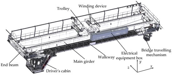
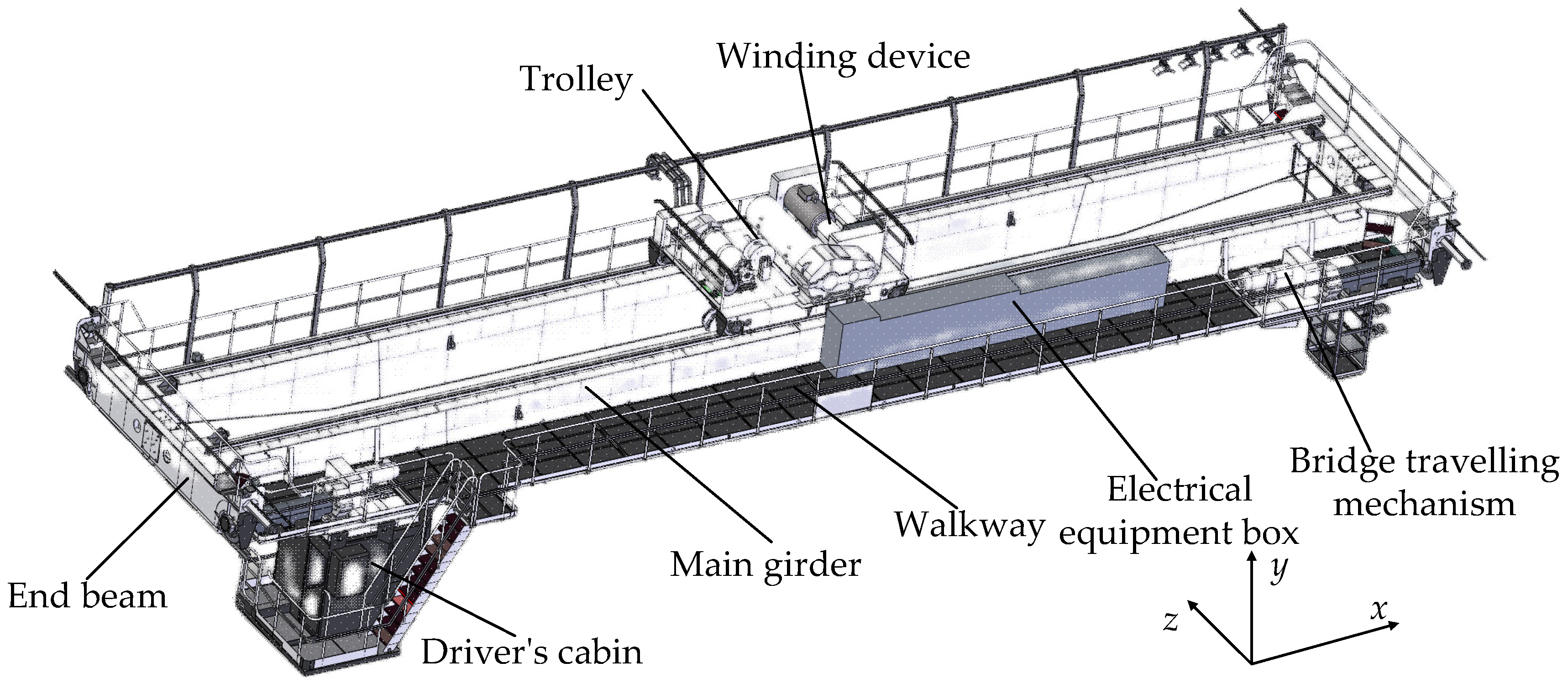
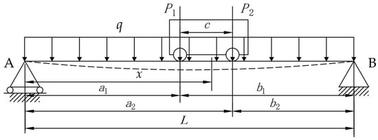
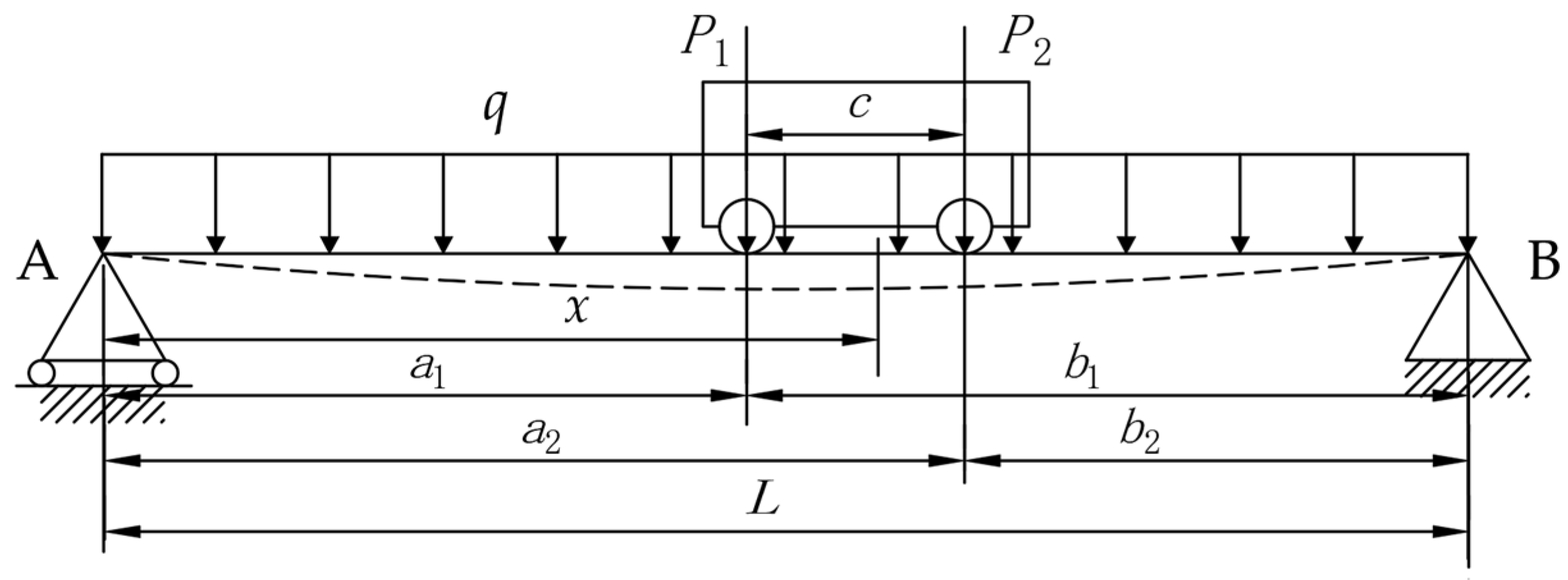
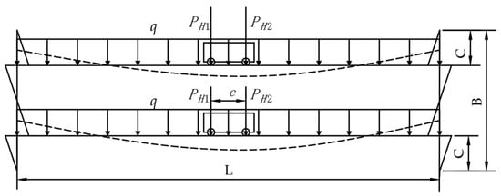
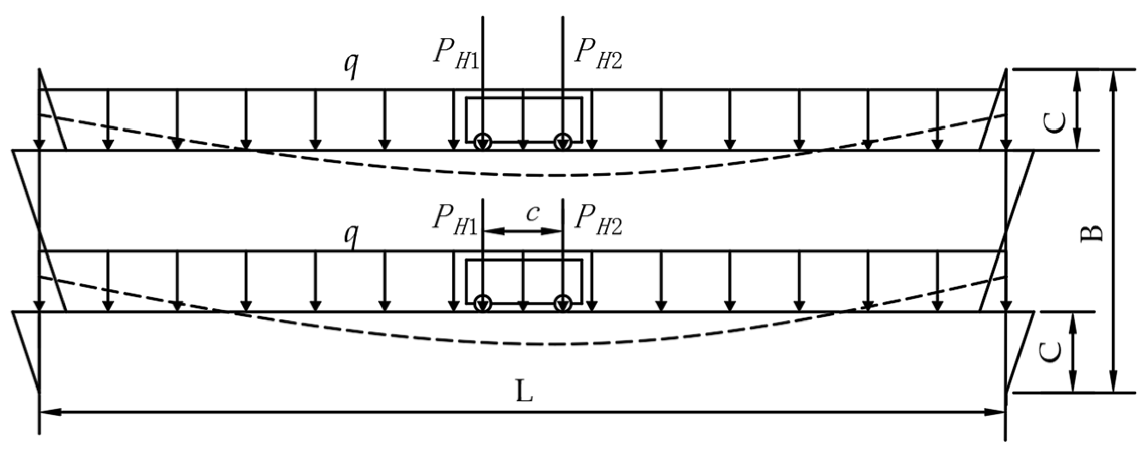
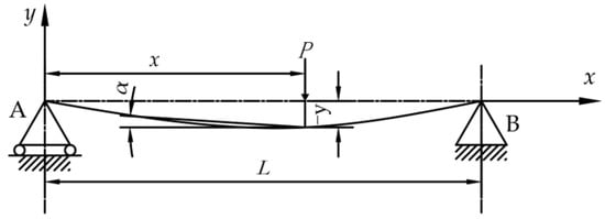
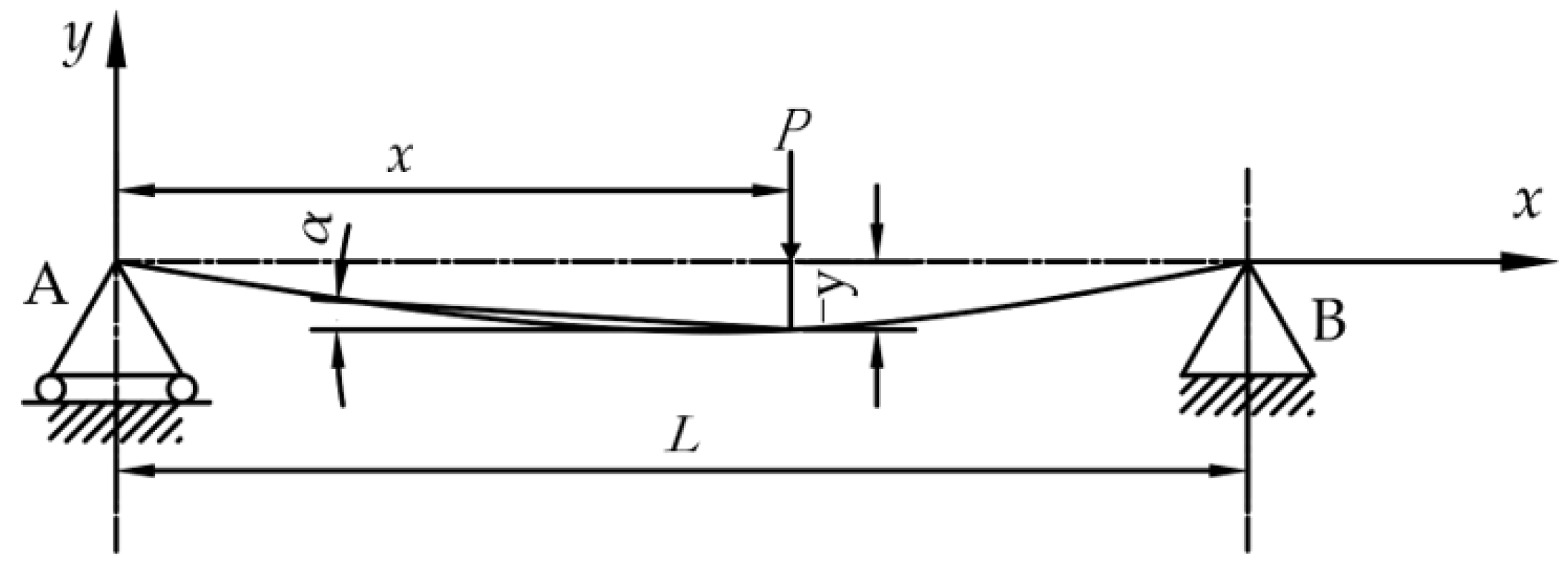
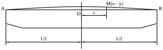
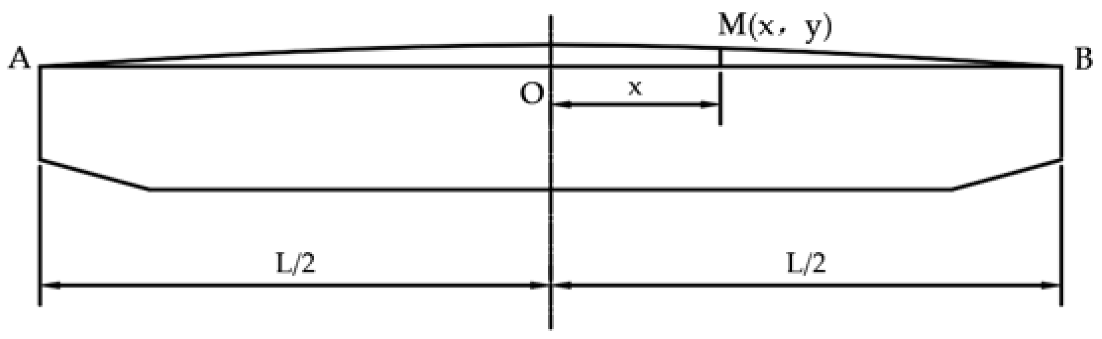
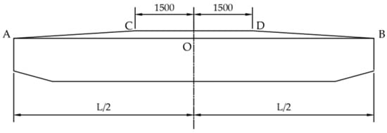
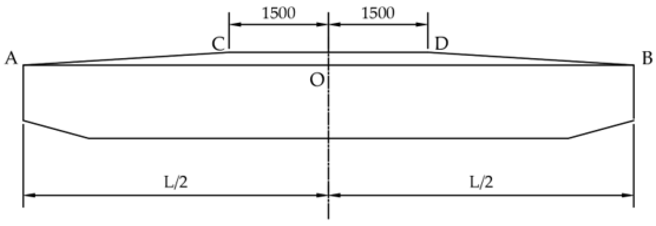
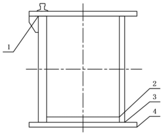
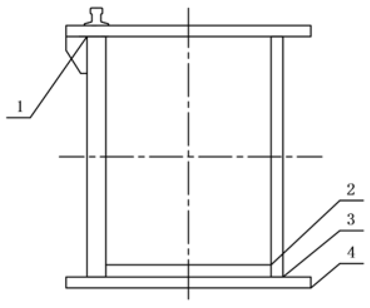
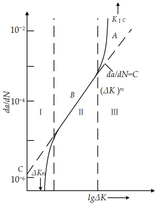
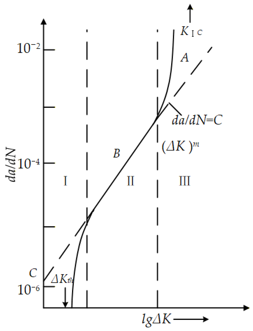
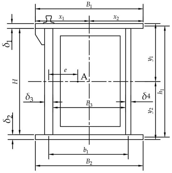
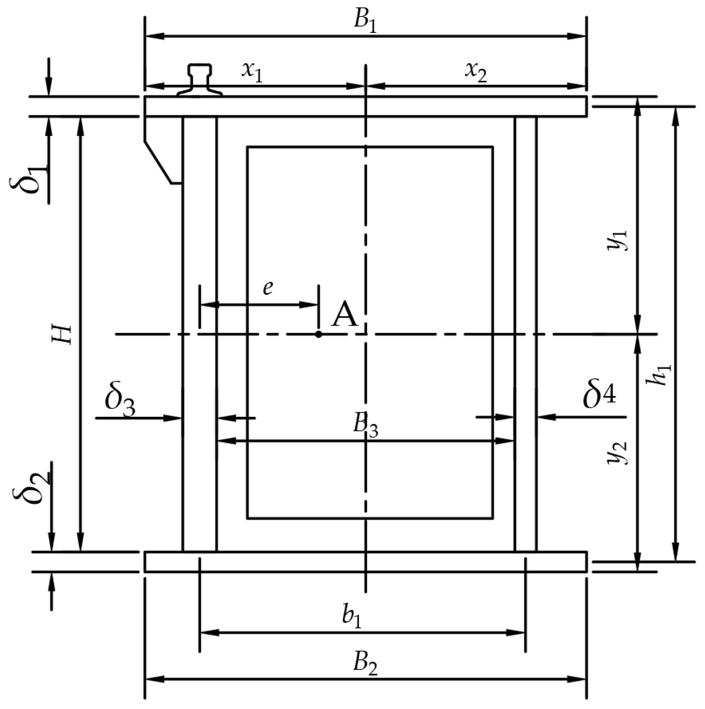
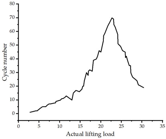
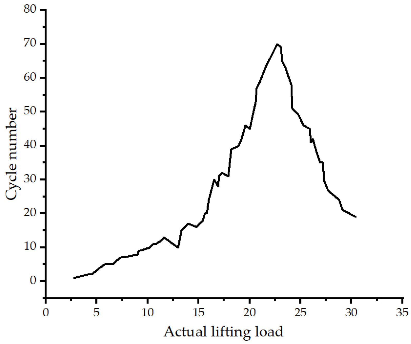
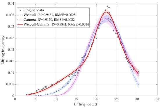
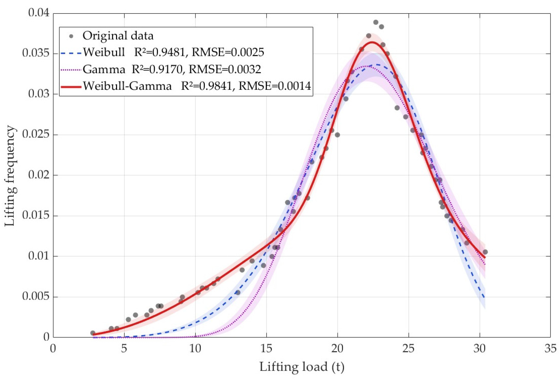
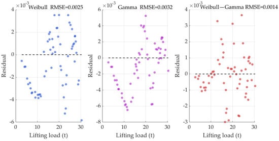
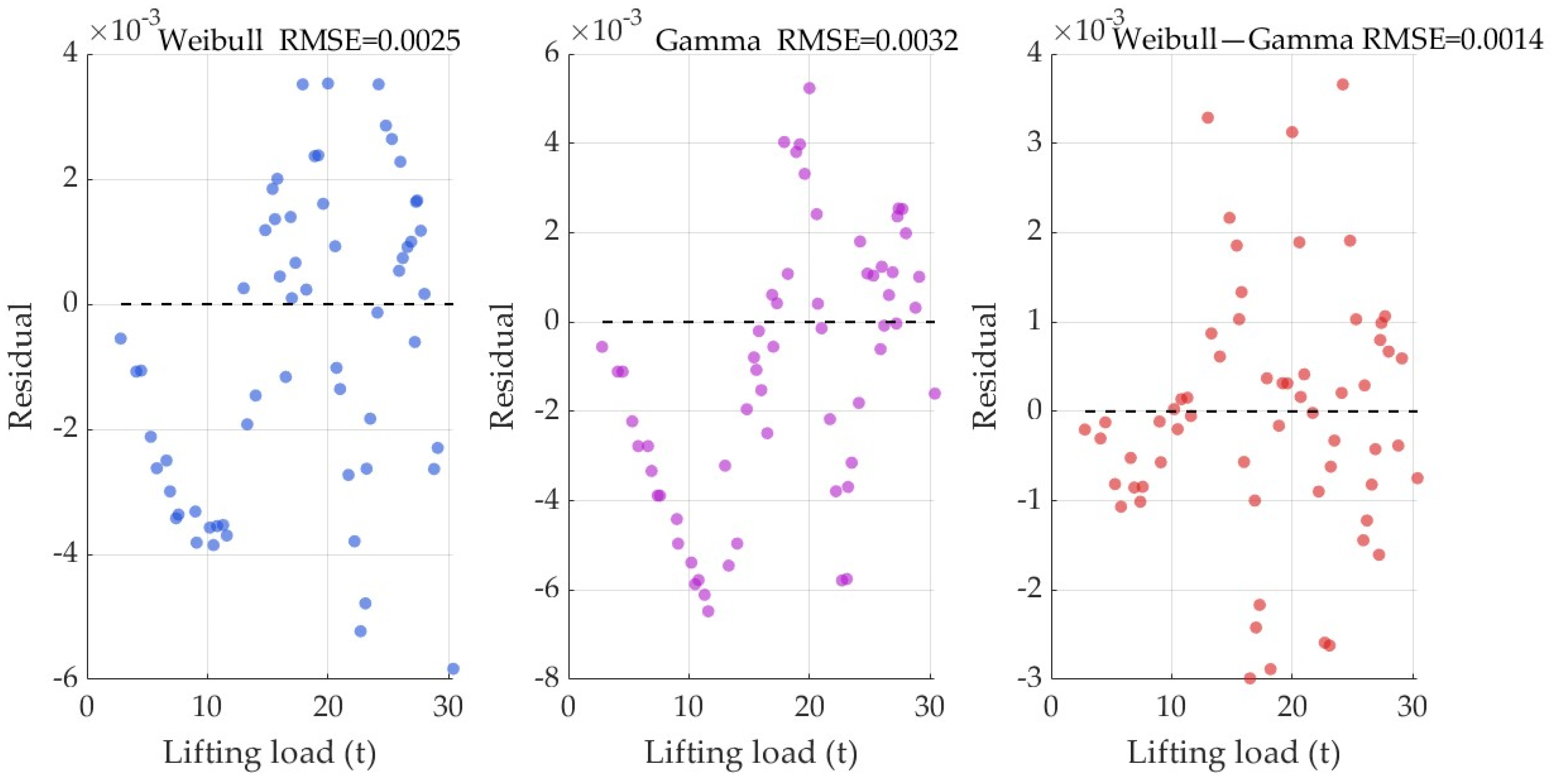
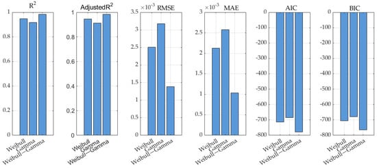
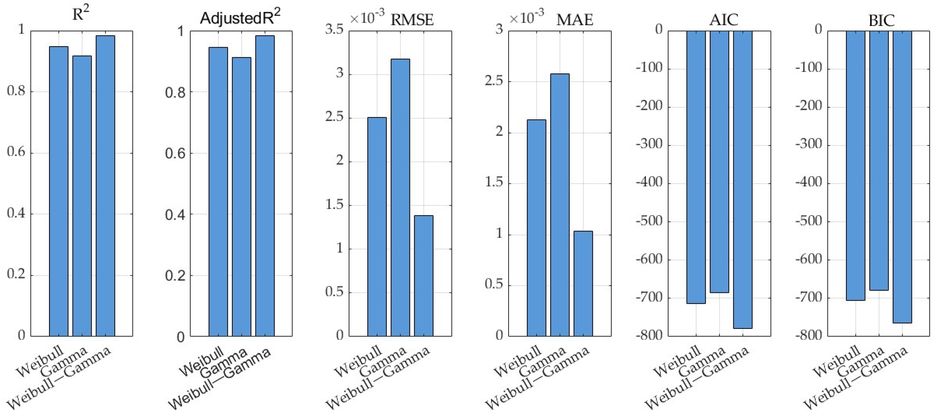
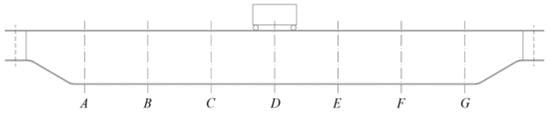
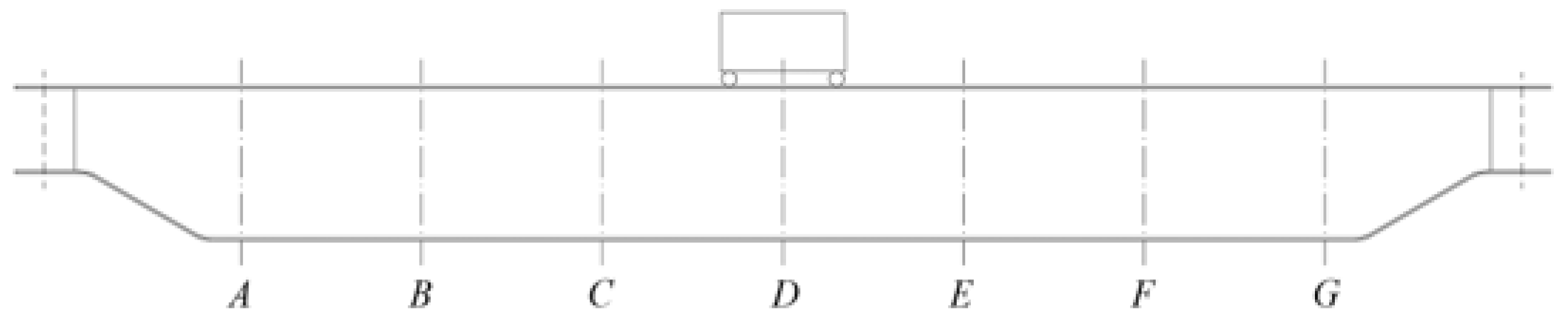
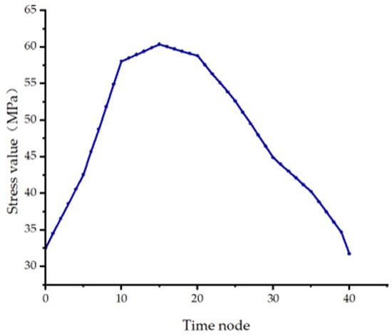
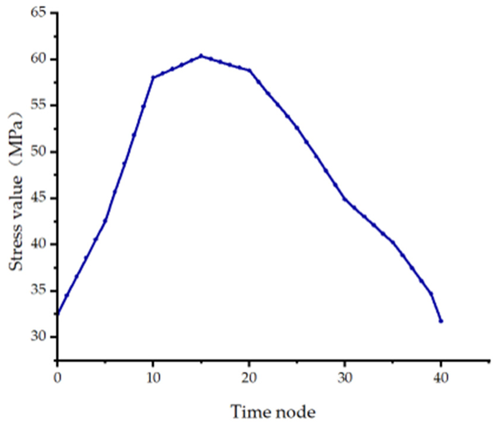
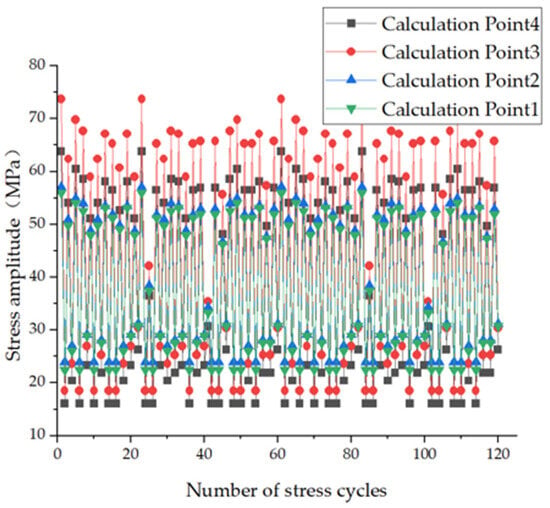
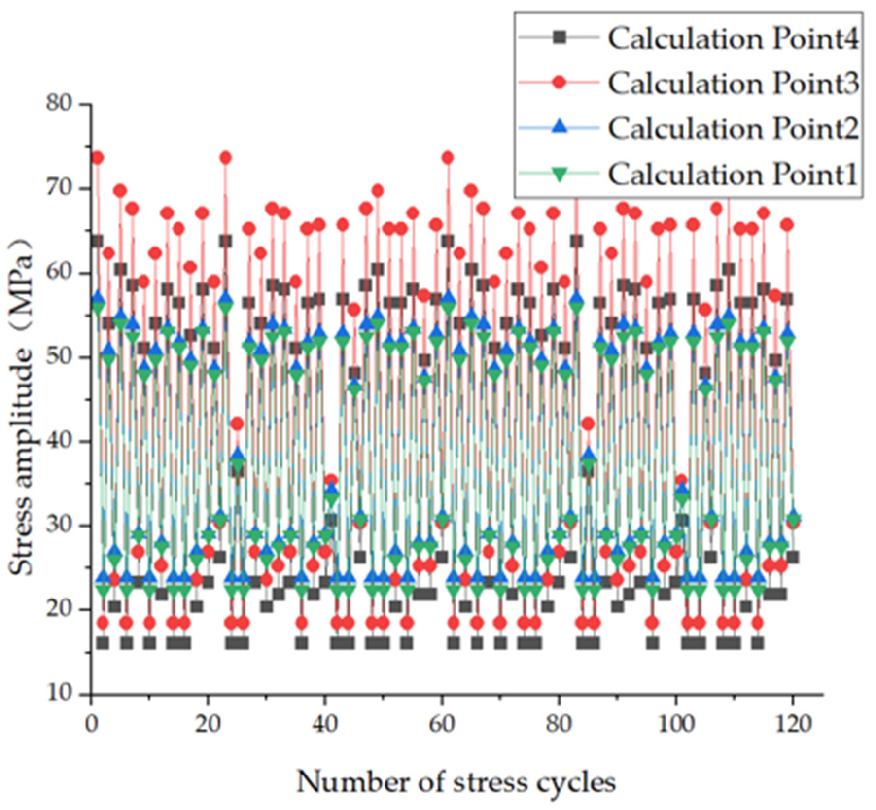
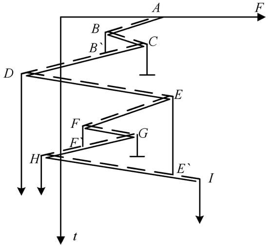
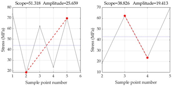
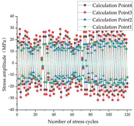
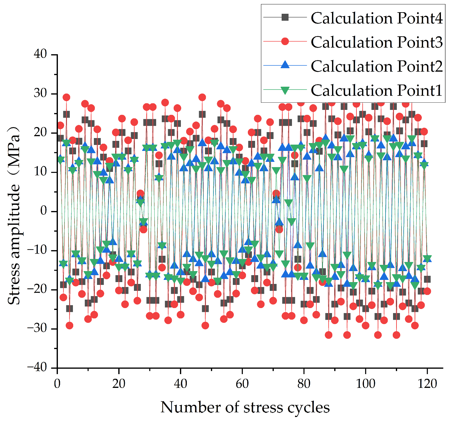
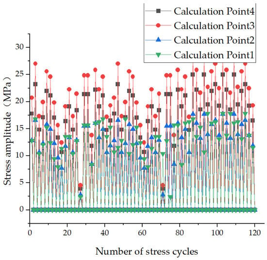
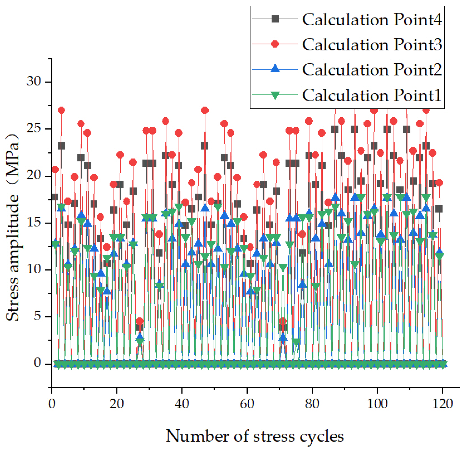
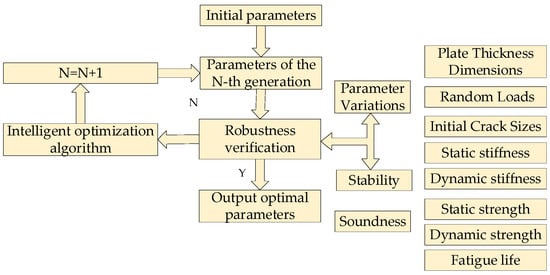
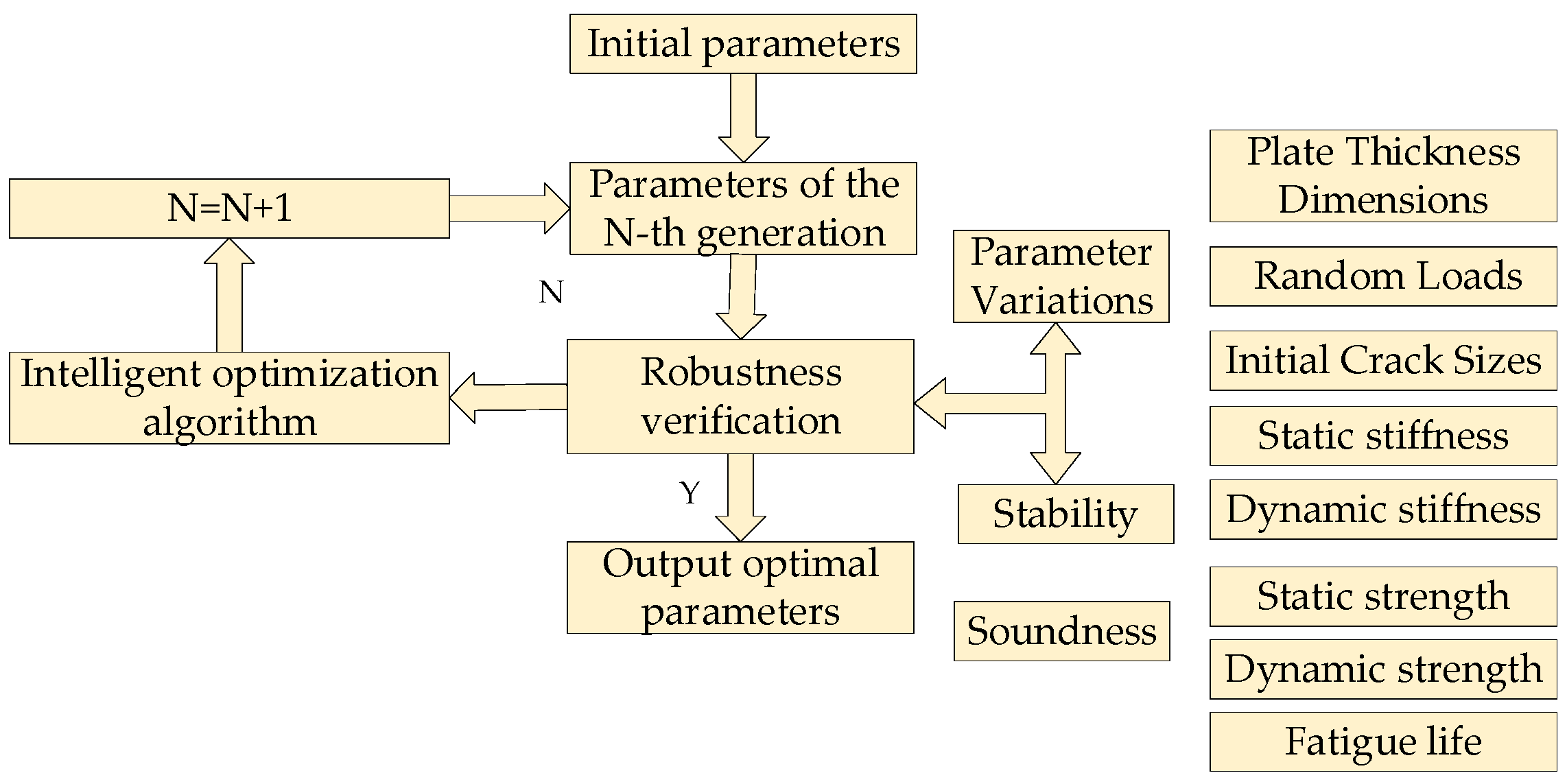
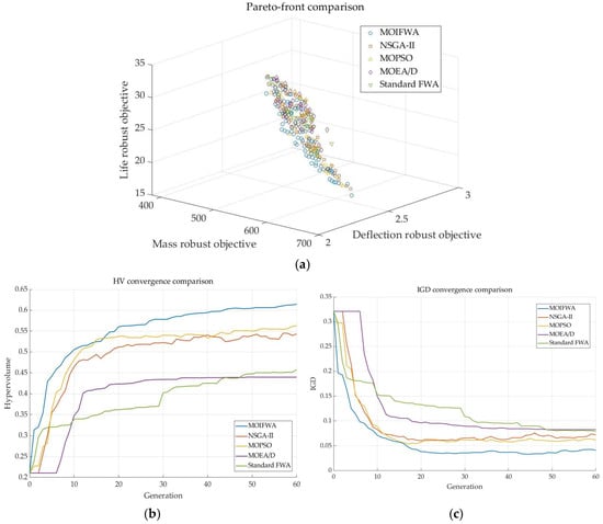
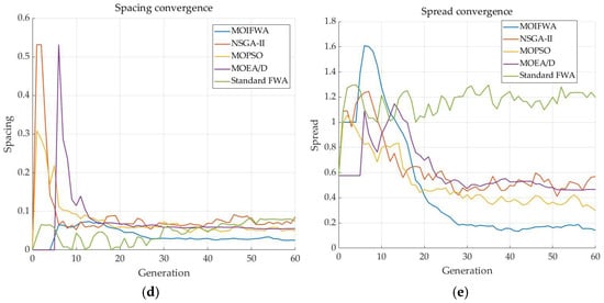
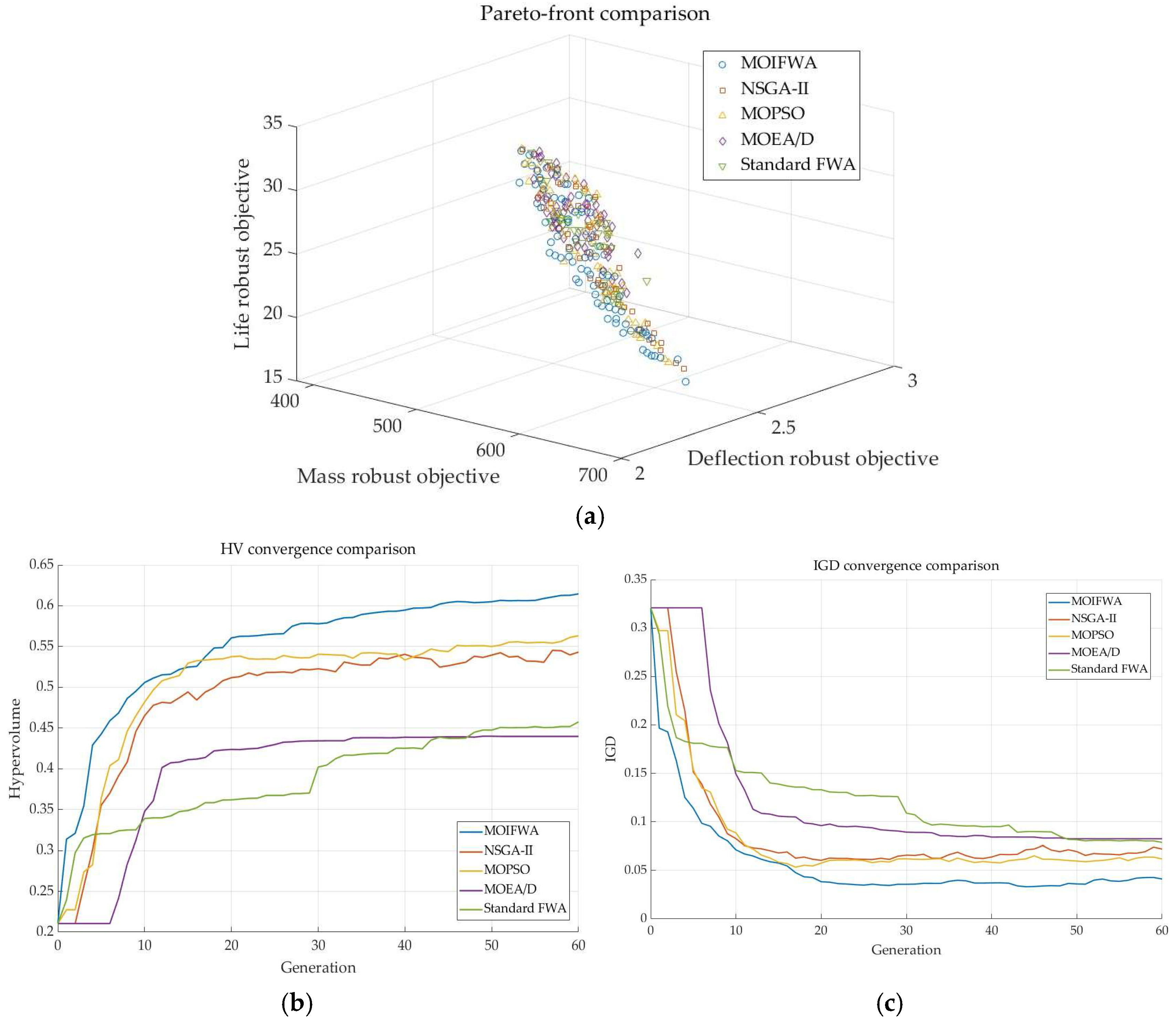
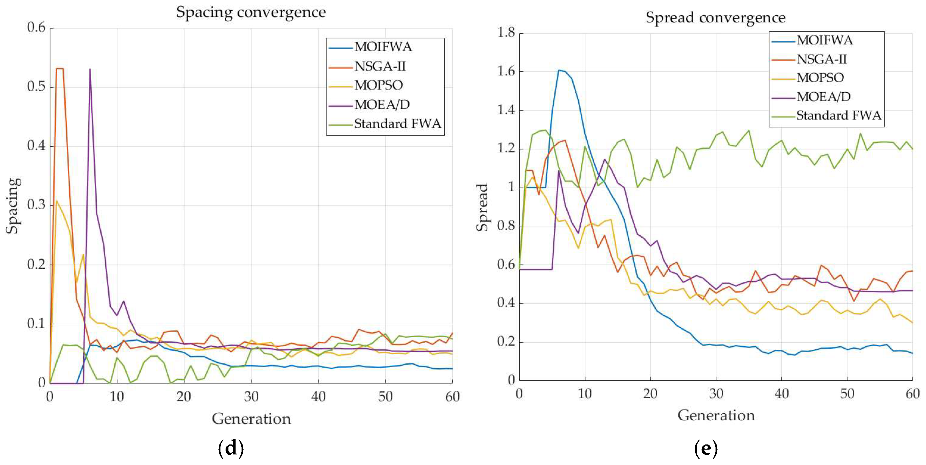
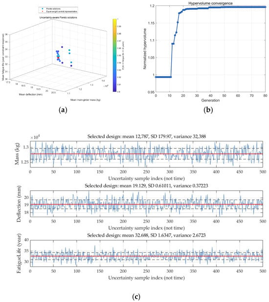
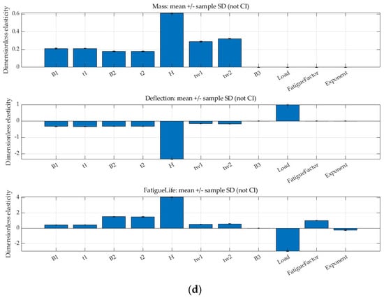
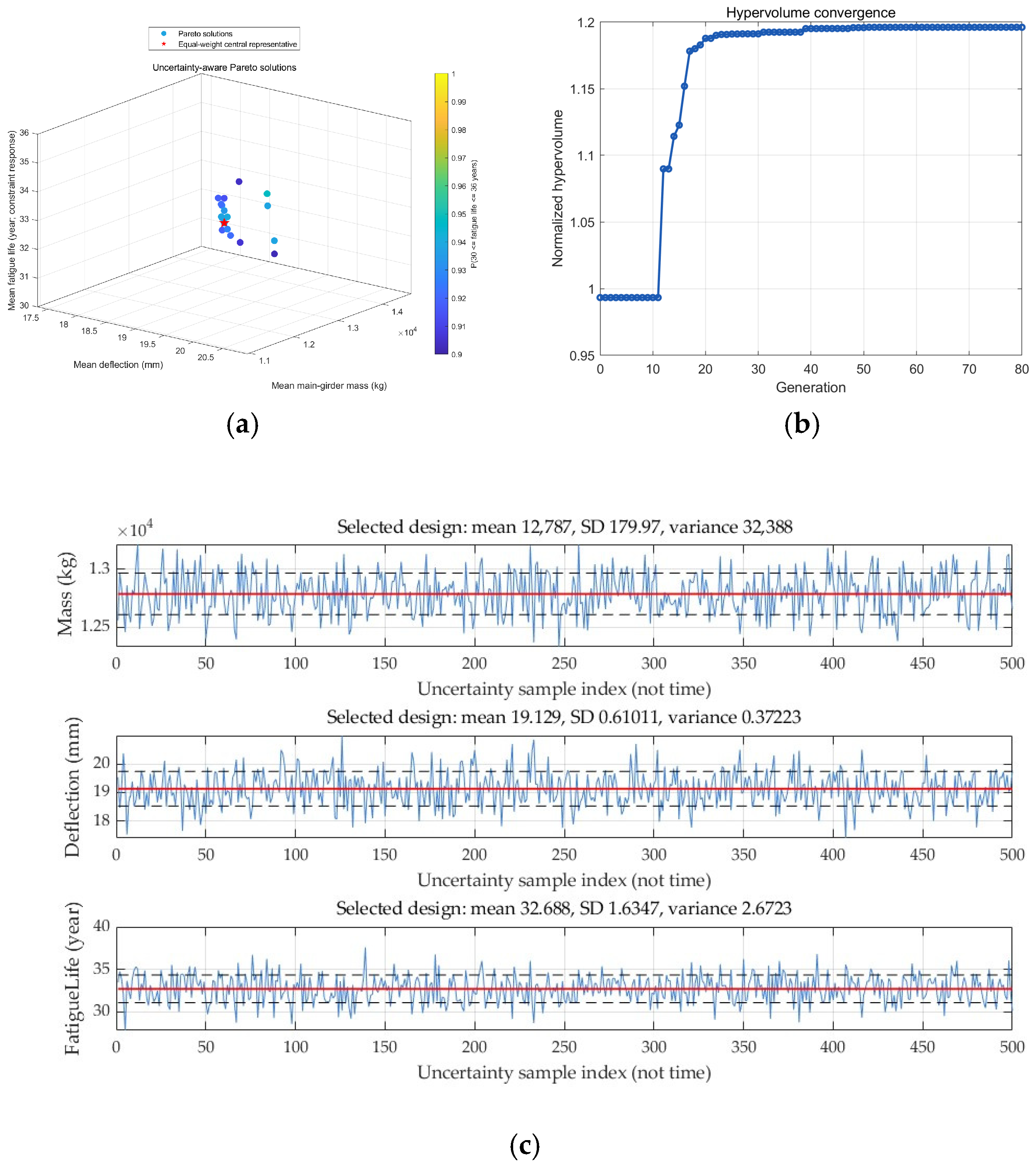
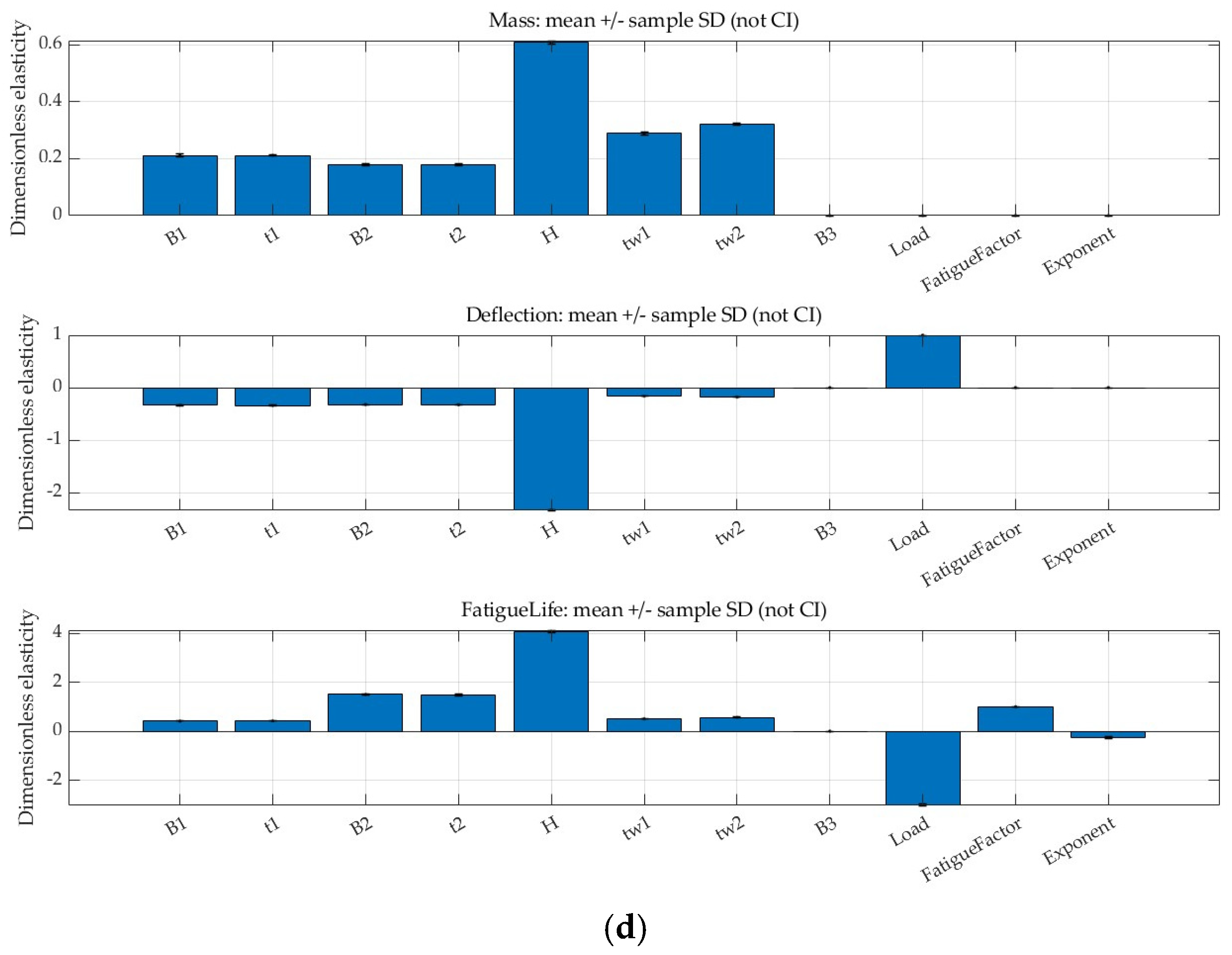
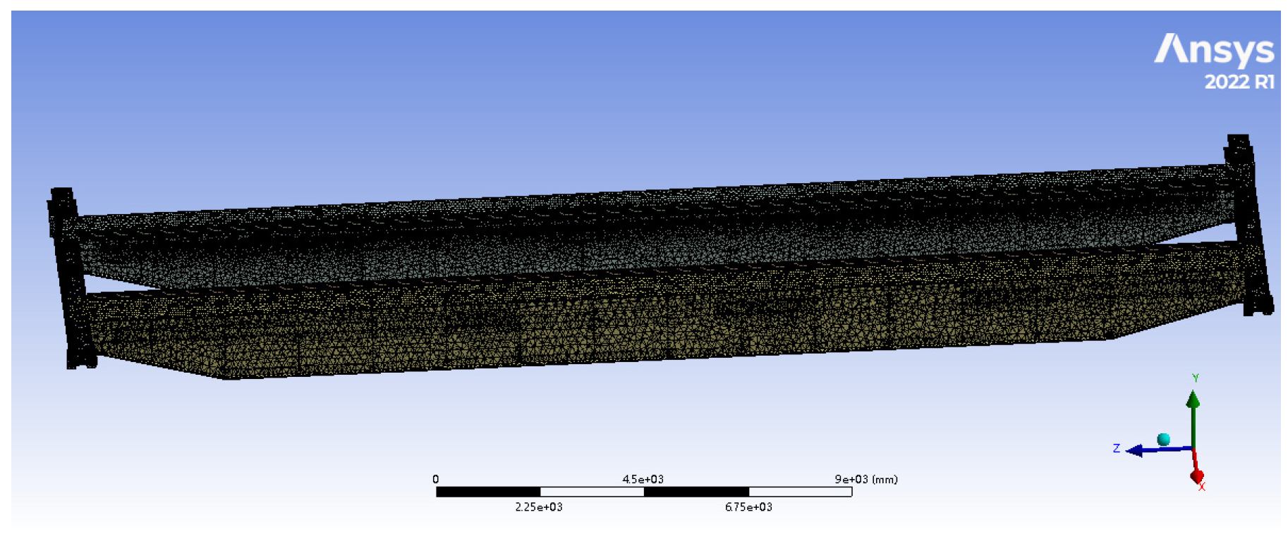
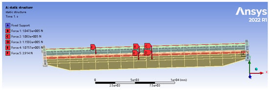
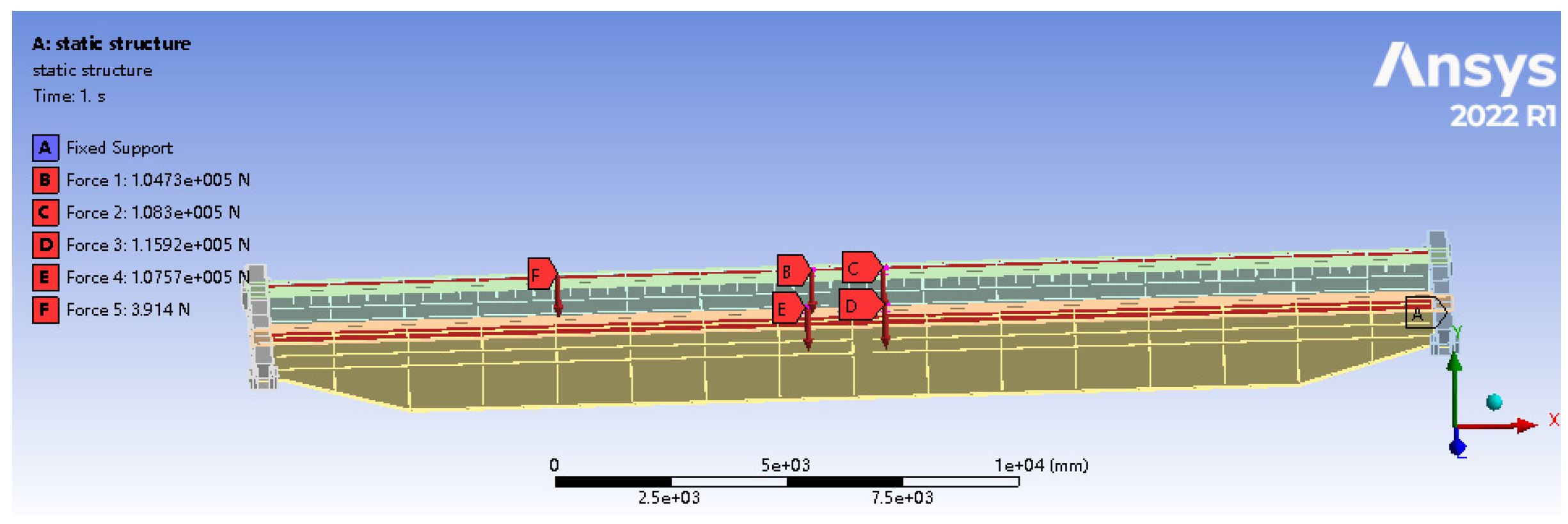
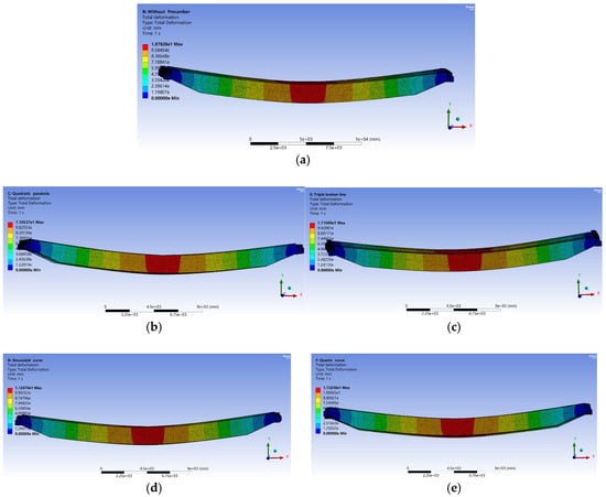
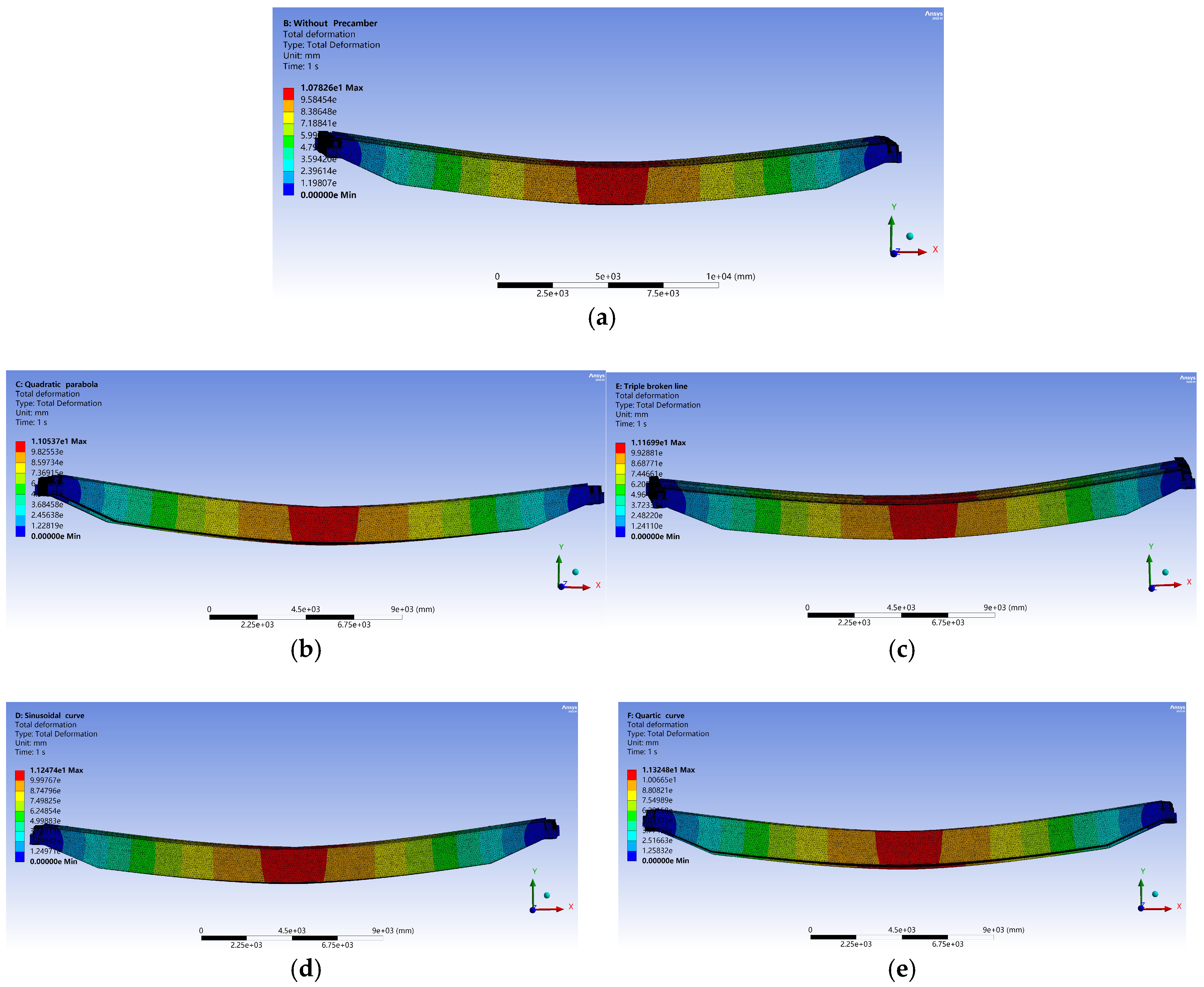
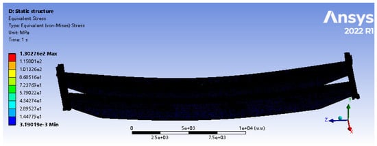
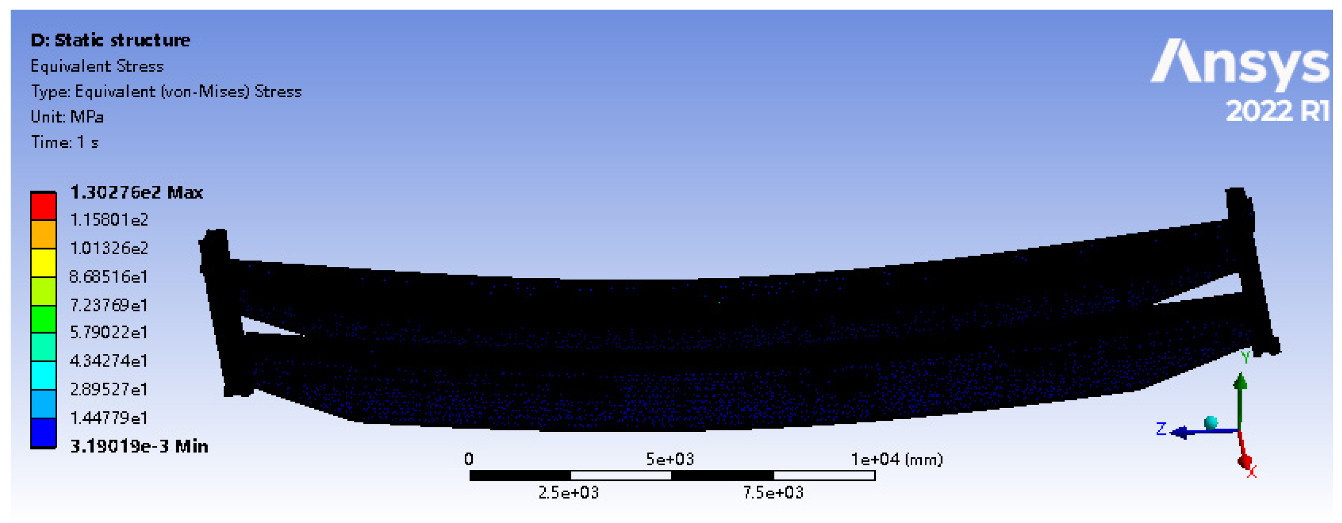
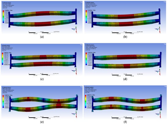
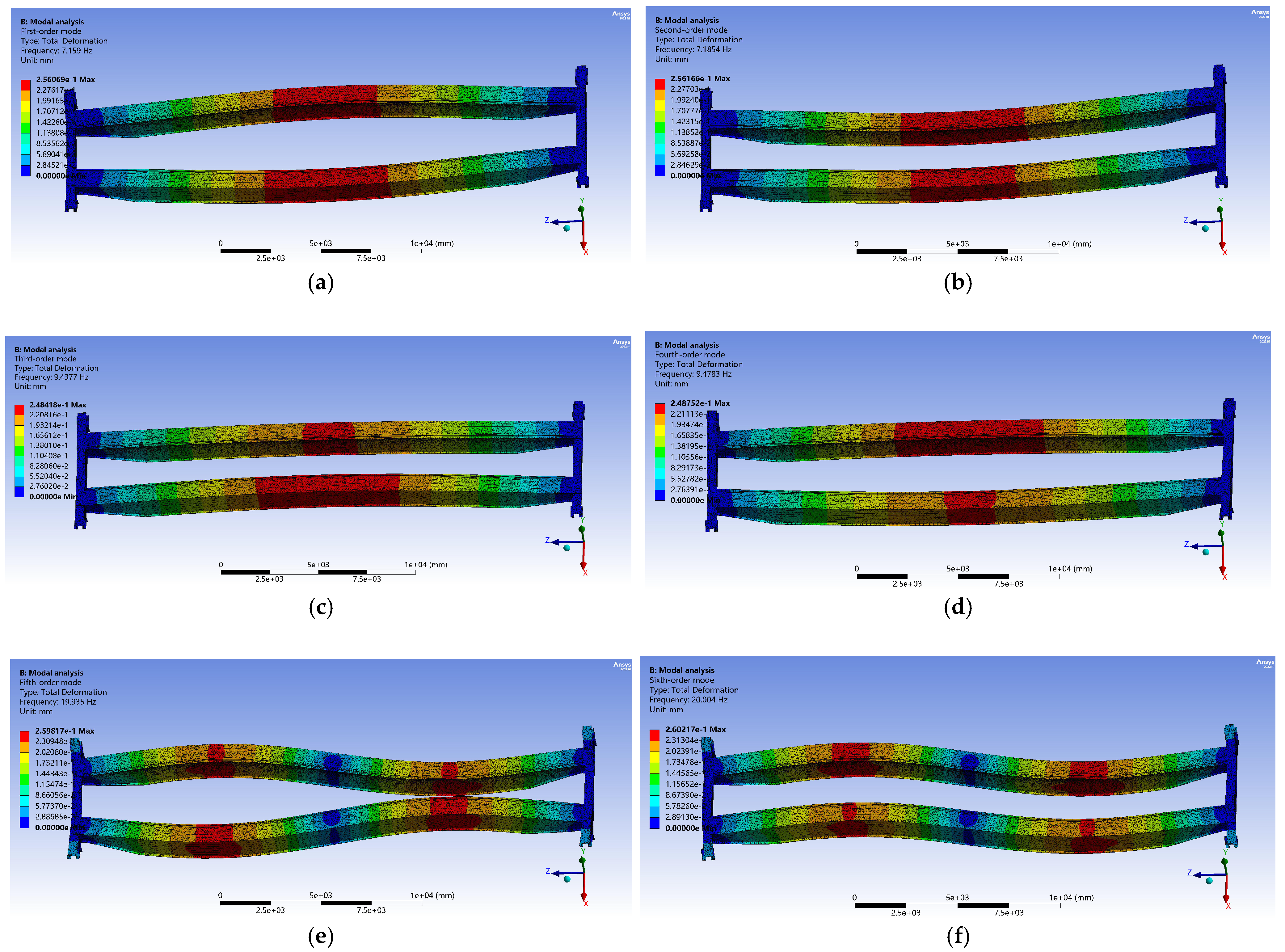
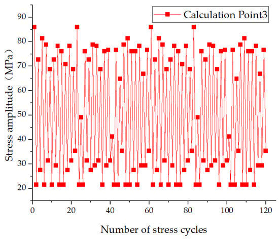
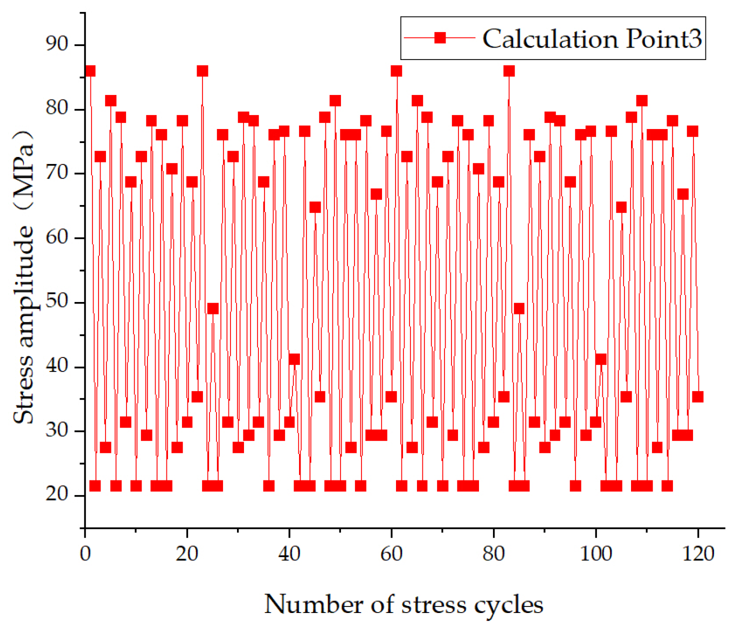
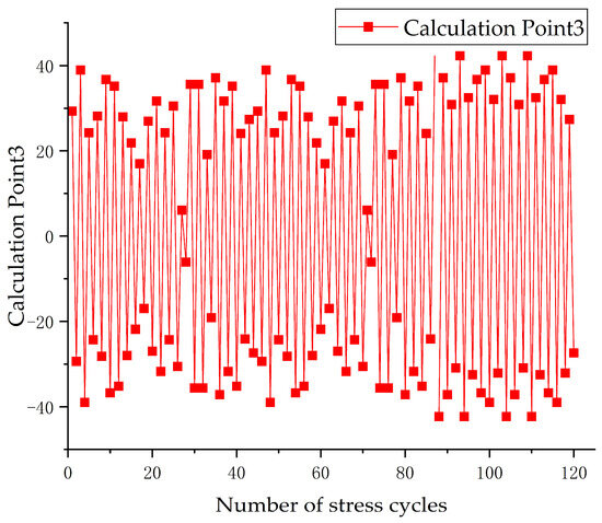
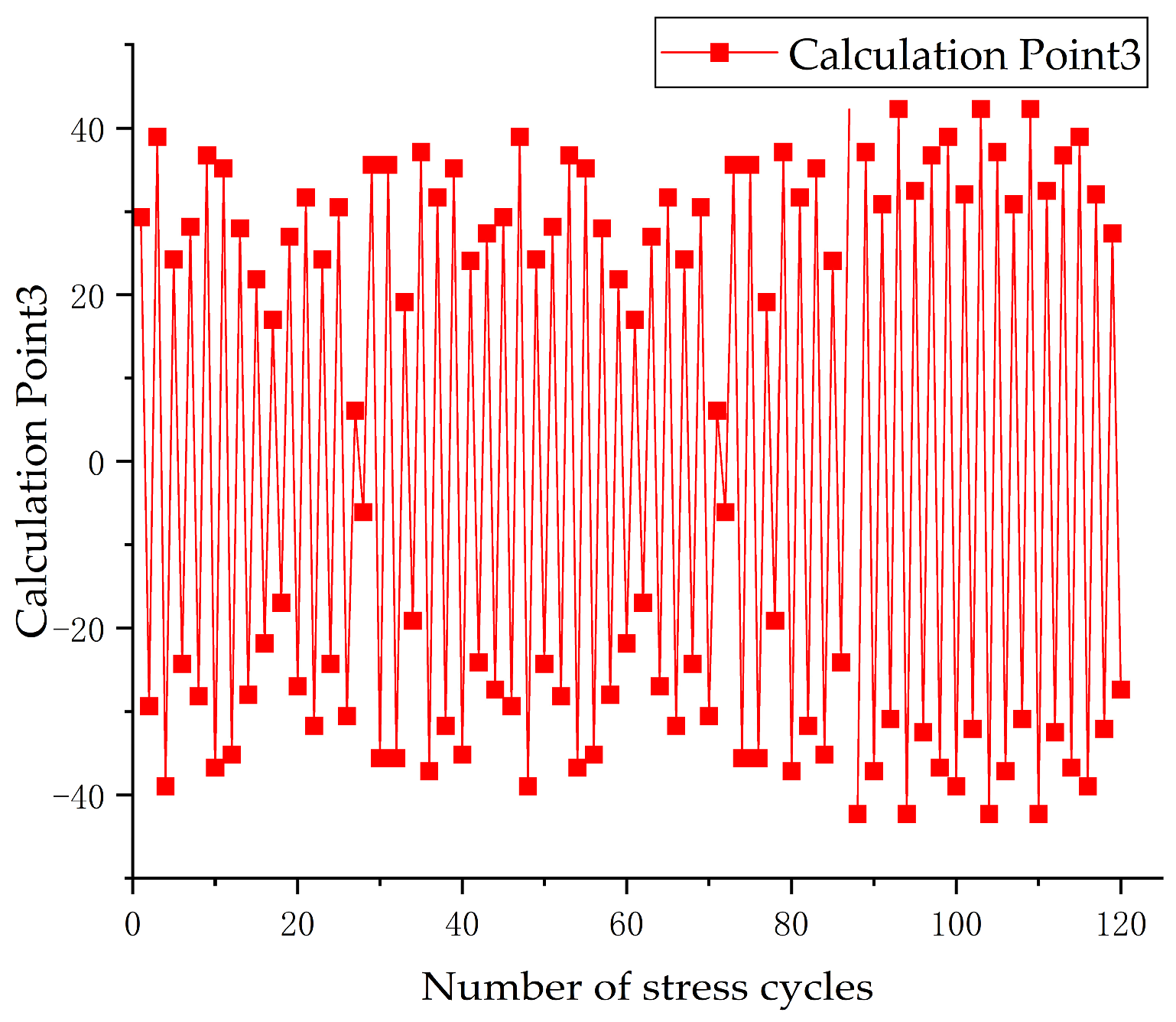
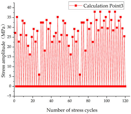
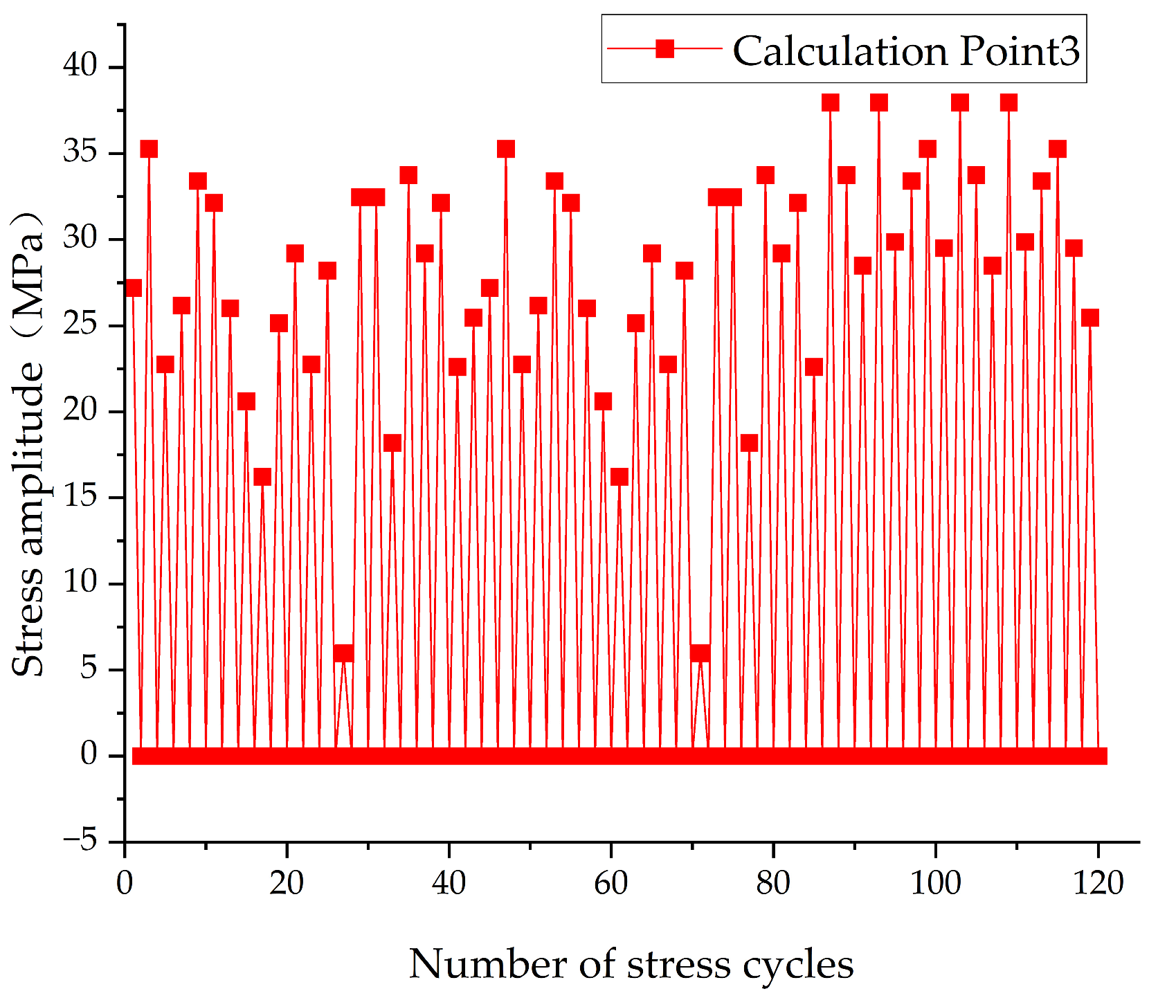
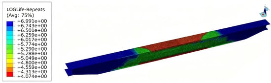
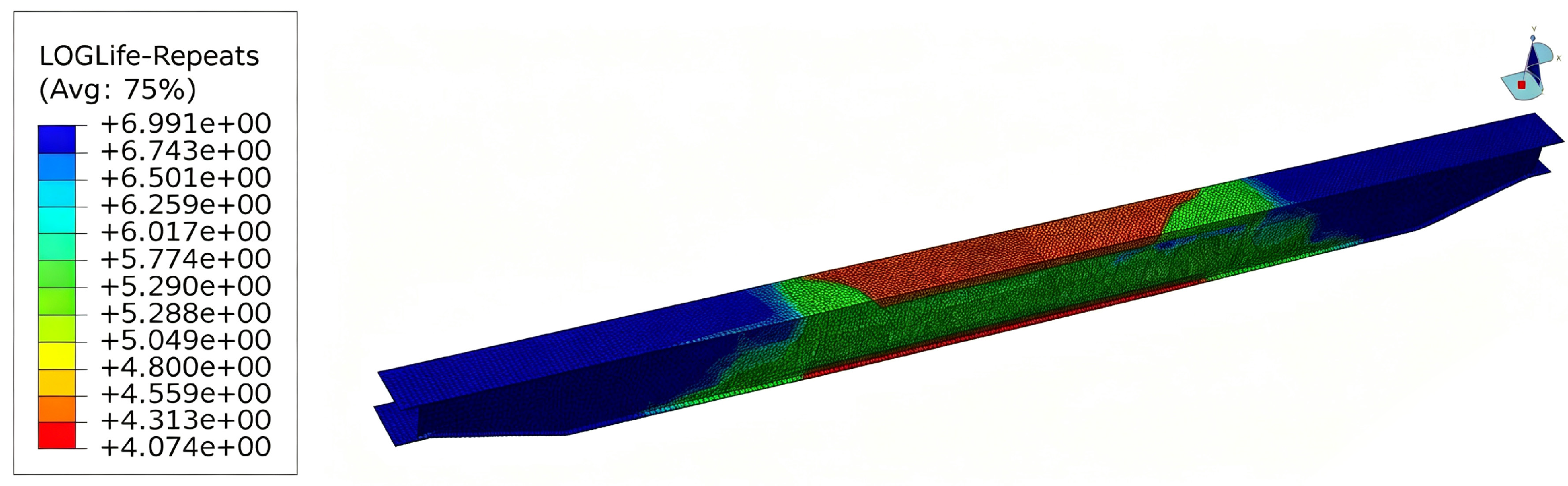

Disclaimer/Publisher’s Note: The statements, opinions and data contained in all publications are solely those of the individual author(s) and contributor(s) and not of MDPI and/or the editor(s). MDPI and/or the editor(s) disclaim responsibility for any injury to people or property resulting from any ideas, methods, instructions or products referred to in the content. |
© 2026 by the authors. Licensee MDPI, Basel, Switzerland. This article is an open access article distributed under the terms and conditions of the Creative Commons Attribution (CC BY) license.