An Anomaly Detection Method for Sliding Bearings Under Electromagnetic Interference Based on an Asymmetric Autoencoder and a Dual-Indicator Diagnostic Plane

Abstract

As core components of marine power systems, sliding bearings directly affect the operational safety of ships. To address the challenges that early weak anomaly features of sliding bearings are easily masked by electromagnetic interference (EMI) and that a single evaluation indicator may respond differently across wear conditions, this paper proposes an asymmetric autoencoder dual-indicator anomaly detection (AADI-AD) method. First, adaptive notch filtering and high-pass filtering are employed to suppress EMI. Then, horizontal and vertical asymmetric convolution kernels are introduced, and an autoencoder is constructed in combination with a dynamic feature allocation mechanism to represent directional time–frequency structures. Finally, a dual-indicator diagnostic plane is established by combining time-domain kurtosis with the mean squared error (MSE) for time–frequency image reconstruction. The experimental results show that the two indicators provide complementary responses across the examined wear conditions and reduce missed detections compared with single-MSE evaluation. These results demonstrate the effectiveness of the proposed method for sliding-bearing anomaly detection under the EMI-contaminated conditions represented by the present experimental platform.

1. Introduction

As key components in marine power systems, sliding bearings directly affect the operational safety of the entire system. Owing to the complex marine environment, bearings are often exposed to severe operating conditions, including impact loads and lubrication fluctuations, which may lead to wear or even failure. Therefore, reliable monitoring of their wear states is necessary to maintain safe ship operation [1,2,3]. When wear occurs in sliding bearings, acoustic emission (AE) technology can be used to collect high-frequency stress wave signals generated by internal friction, and features reflecting bearing anomalies can be extracted from the original AE data for condition monitoring. However, in industrial environments, the high-frequency switching actions of variable-frequency drive motors generate electromagnetic interference (EMI), which can be coupled into AE sensors and mask the anomaly features of bearings, making effective feature extraction difficult [4,5,6]. When training anomaly detection models using extracted features, most existing mainstream methods rely on a single evaluation indicator as the decision criterion, making it difficult to adapt to the feature differences among different wear stages. Therefore, constructing an anomaly detection model with both anti-interference capability and reliable detection performance across different wear stages in EMI environments has gradually become an important research direction in anomaly detection.

To address the difficulty of feature extraction in noisy environments, a range of data-driven approaches has been applied to anomaly detection [7,8,9]. The isolation forest (IF) algorithm proposed by Liu et al. [10] constructs random isolation trees and is widely used to identify anomalies in industrial time-series data. Shin et al. [11] characterized normal equipment behavior by using a one-class support vector machine (One-Class SVM) to establish an operating boundary within a multidimensional feature space. However, most of these methods rely on manually extracted features and lack automatic feature extraction capability. To overcome this limitation, Wen et al. [12] introduced a convolutional neural network (CNN) into this field, enabling end-to-end nonlinear feature learning. Subsequent research has explored several strategies for limiting noise-induced feature distortion and increasing model resilience to interference. Based on a variational denoising autoencoder (VDAE), Yan et al. [13] proposed an optimized stacked variational denoising autoencoder (OSVDAE), which effectively suppresses strong background noise by optimizing the reconstruction probability space. Shi et al. [14] introduced multi-scale large convolution kernels and a gated recurrent unit (GRU) into Deep Convolutional Neural Networks with Wide First-layer Kernels (WDCNN), significantly enhancing the model’s feature extraction and anti-interference capabilities under complex strong-noise conditions. Lu et al. [15] constructed a dual-branch convolutional capsule network, which adaptively extracts fault type and damage scale features, effectively overcoming the degradation of diagnostic accuracy caused by strong background noise masking. In addition, for complex operating conditions and cross-domain diagnosis, Ding et al. [16] applied Transformer architectures to time-frequency representations, whereas Tang et al. [17] used them for visual images. The extracted deep features enabled accurate fault-category identification under variable loads and strong noise interference. Li et al. [18] constructed a domain adversarial graph convolutional network (DAGCN) that integrates graph structure modeling and adversarial learning to mitigate feature distribution discrepancies across variable operating conditions. Ragab et al. [19] developed a conditional contrastive domain generalization (CCDG) method that learns domain-invariant features by maximizing mutual information among same-class samples from different domains. This mechanism improves model generalization and robustness in unknown target domains.

Despite their strong feature-extraction performance, these models generally require substantial labeled anomaly data. Because anomaly samples are limited in many industrial applications, reconstruction-based autoencoder models remain widely used for anomaly detection. However, when mainstream autoencoder architectures are directly applied to wear monitoring of sliding bearings, their reliance on mean squared error (MSE) as a single evaluation indicator can make it difficult to distinguish anomaly features across different wear conditions. Gao et al. [20] pointed out that redundant network capacity can cause overgeneralization when evaluating the anomaly detection performance of autoencoders, allowing models to reconstruct anomaly samples with relatively high accuracy. Huang et al. [21] further demonstrated that conventional autoencoders tend to produce smooth fitting and excessive reconstruction of unknown anomaly features. As a global average error metric, MSE may dilute local weak transient impulses generated by early wear. Studies by Antoni [22] and Randall [23] have shown that kurtosis is sensitive to transient impulses and can complement reconstruction error. As transient impulses become denser, kurtosis may decrease; however, its actual variation depends on the operating conditions and measurement characteristics. MSE and kurtosis can be combined into a single score through linear weighting, but compressing indicators with different responses into one scalar score may reduce the contribution of an indicator at a particular degradation stage. Section 4.4 therefore compares a linear MSE–kurtosis score-fusion baseline with the OR-based joint decision strategy adopted in this study.

Compared with three related categories of methods, the novelty of AADI-AD lies in its integrated processing and decision framework for sliding-bearing monitoring across different wear conditions in the presence of variable-frequency-drive EMI. Denoising autoencoders mainly reduce the influence of noise through reconstruction learning, whereas the proposed method first applies adaptive notch filtering according to the identified EMI fundamental frequency and employs high-pass filtering to suppress low-frequency mechanical and environmental background components. It subsequently uses 1 × 9 and 9 × 1 directional convolutional branches with dynamic weighting to represent horizontally extended structures and vertically localized transient structures. Unlike physics-informed diagnosis methods that introduce governing equations or physical constraints into the training objective [24,25,26], the proposed method uses known EMI frequency information in signal preprocessing and employs time-domain kurtosis as an anomaly indicator parallel to the reconstruction MSE. In contrast to weighted-score multi-indicator strategies that linearly combine multiple indicators into a single score, AADI-AD retains separate thresholds for MSE and kurtosis and combines their decisions using an OR rule, thereby preserving their complementary responses under different wear conditions. The fundamental novelty therefore lies in the coordinated design of directional time–frequency feature representation and MSE–kurtosis joint decision-making for variable-frequency-drive EMI contamination and different wear conditions.

To address the problems that early weak features are easily masked in the presence of EMI and that a single MSE indicator has a missed-detection blind spot in early-stage anomaly detection, this paper proposes an asymmetric autoencoder dual-indicator anomaly detection (AADI-AD) method. The subsequent sections are arranged as follows. Section 2 details the proposed framework, covering the preprocessing strategy, the architecture of the asymmetric-kernel autoencoder, and the construction of the dual-indicator diagnostic plane. Section 3 describes the experimental setup and the procedure used for data acquisition. Section 4 analyzes the results obtained from the sliding-bearing experiments and evaluates the proposed method under the EMI-contaminated conditions represented by the present experimental platform. The principal findings are summarized in Section 5.

2. Asymmetric Autoencoder Dual-Indicator Anomaly Detection Method

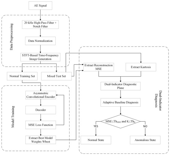
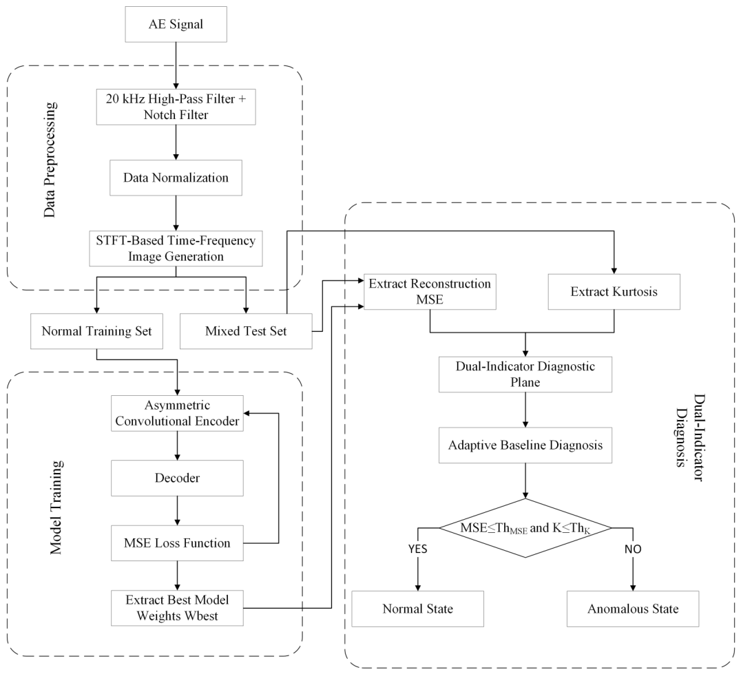
To address the challenges that early weak transient signals of sliding bearings are easily masked and that a single feature is insufficient to characterize different wear conditions, this paper proposes an asymmetric autoencoder dual-indicator anomaly detection method, as shown in Figure 1.

Figure 1. Flowchart of the proposed anomaly detection method.

2.1. Data Preprocessing

Traditional digital signal processing techniques usually attenuate electromagnetic interference (EMI) through band-pass filtering or wavelet threshold denoising. However, inappropriate filtering may distort transient signals [27,28]. This study therefore combines targeted digital filtering with an autoencoder-based anomaly detector.

After amplitude conversion and detrending of the original acoustic emission (AE) signal, Welch power spectral density estimation was first used to identify the actual fundamental frequency of the variable-frequency-drive interference. The search was centered at the nominal frequency of 15 kHz within a range of $\pm 500$ Hz. When the maximum peak power within this interval exceeded five times the median background power, the corresponding peak frequency was selected as the EMI fundamental; otherwise, the nominal value of 15 kHz was retained. A second-order infinite impulse response (IIR) notch filter with a quality factor of $Q=30$ was subsequently applied at the identified fundamental frequency using forward–backward filtering to obtain a zero-phase response.

After suppression of the fundamental component, a fourth-order Butterworth high-pass filter with a cutoff frequency of $f_c=20\mathrm{kHz}$ was applied in second-order-section form using the same forward–backward procedure. Its amplitude-frequency response satisfies

$${\left|H\left(j\omega \right)\right|}^2={\displaystyle \frac{1}{1+{\left(\frac{2\pi f_c}{\omega }\right)}^8}},$$

(1)

where $H\left(j\omega \right)$ denotes the amplitude-frequency response of the filter, $\omega$ denotes the signal angular frequency, and $f_c$ specifies the cutoff frequency. The continuous signal was then divided into non-overlapping 0.5 s windows.

To further suppress periodic EMI harmonics above the high-pass cutoff, frequency-domain magnitude interpolation was performed on each signal window. Before the fast Fourier transform (FFT), a Tukey window with a shape parameter of 0.02 was applied to reduce boundary effects. The harmonic centers were defined as integer multiples of the identified fundamental, with up to eight harmonics considered within the Nyquist frequency. At the sampling frequency of 216 kHz, the processed harmonic centers were approximately 30, 45, 60, 75, 90, and 105 kHz. The half-bandwidth of the k-th harmonic band was defined as

$$B_k=\min \{400[1+1.5(k-1)],3000\}\mathrm{Hz}.$$

(2)

Within each target harmonic band, the spectral magnitudes were linearly interpolated from the median magnitudes of the adjacent reference bands, while the original phase angles were retained. The time-domain signal was then recovered through the inverse FFT.

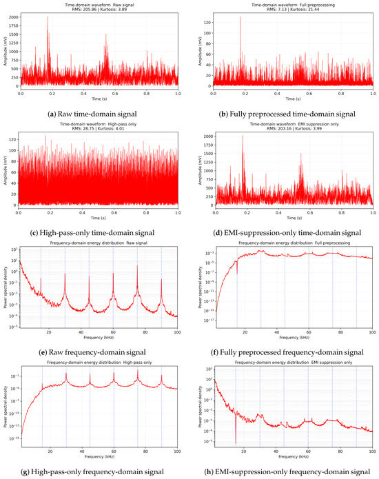
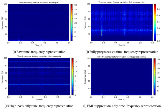
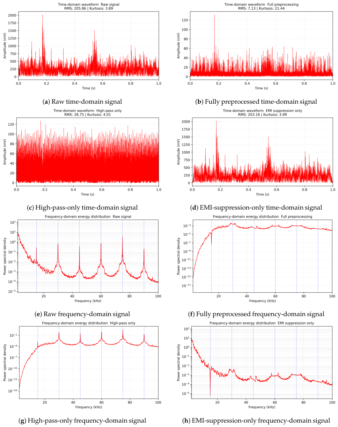
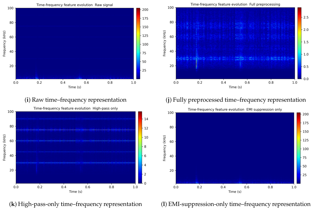
Before converting the signal into time–frequency images as input to the neural network, data normalization is required. Considering that the AE energy of sliding bearings spans several orders of magnitude at different wear stages, conventional slice-level normalization may erase the true energy-gradient differences. Therefore, this paper avoids local compression and adopts a global physical energy scale. Specifically, the 99.9th percentile of the amplitude of the normal data in the training set is extracted as a unified reference, thereby achieving global proportional scaling for all slices. The normalized signal is then transformed into two-dimensional time-frequency images using the short-time Fourier transform (STFT). The data preprocessing results are compared in Figure 2.

Figure 2. Representative AE signal acquired at 60 rpm under four preprocessing configurations.

To distinguish the effects of high-pass filtering and EMI suppression on RMS and kurtosis, an ablation analysis was conducted on the existing representative 60 rpm AE signal using four preprocessing configurations: raw signal, high-pass filtering only, EMI suppression only, and full preprocessing. The RMS and kurtosis of the raw signal were 205.86 and 3.89, respectively. The corresponding values were 28.75 and 4.01 after high-pass filtering only, 203.16 and 3.99 after EMI suppression only, and 7.13 and 21.44 after full preprocessing. High-pass filtering alone primarily reduced the low-frequency and broadband background energy, while the periodic EMI harmonics remained. EMI suppression alone attenuated the component at approximately 15 kHz and its harmonics, while the low-frequency background remained. Full preprocessing reduced both background and periodic interference energy while retaining localized transient components in the time-domain and time–frequency representations.

The kurtosis distributions before and after full preprocessing were summarized over all 3860 existing non-overlapping signal windows using the median and interquartile range (IQR), as reported in Table 1. After full preprocessing, the median kurtosis values for Labels 0, 1, and 2 were 5.68, 14.90, and 15.17, respectively. The abnormal and healthy states therefore retained different kurtosis distributions after the same preprocessing procedure, although preprocessing also changed the numerical kurtosis baseline. Accordingly, kurtosis is treated as a statistical descriptor of signal impulsiveness and is used jointly with reconstruction error for anomaly detection.

Table 1. Window-wise kurtosis distributions before and after full preprocessing.

Wear Condition	Windows	Raw Kurtosis, Median [IQR]	After Full Preprocessing, Median [IQR]
Healthy (Label 0)	2261	2.85 [2.63, 3.01]	5.68 [5.27, 6.47]
Mild wear (Label 1)	802	5.55 [3.47, 11.32]	14.90 [12.93, 30.49]
Severe wear (Label 2)	797	3.68 [3.29, 8.84]	15.17 [12.11, 17.39]

2.2. Asymmetric Convolution Kernel Autoencoder

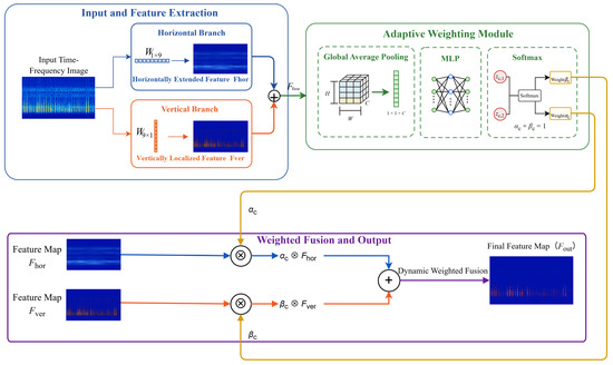
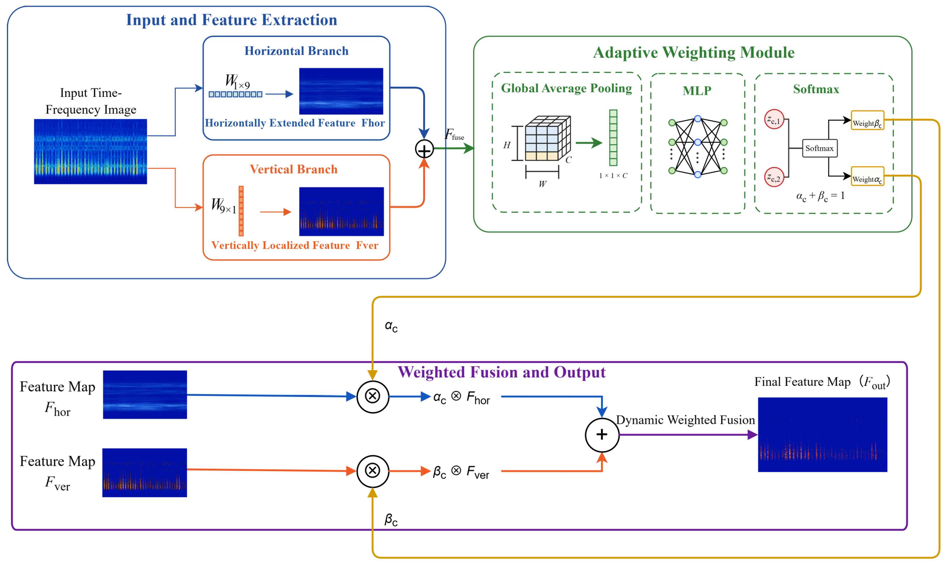
To enhance the representation of time–frequency structures with different orientations, this paper constructs an autoencoder that integrates feature extraction based on asymmetric convolution kernels (ACK) and dynamic weighted fusion. Figure 3 illustrates the complete architecture. The input features are processed by two directional asymmetric convolutional branches. Global average pooling, a multilayer perceptron (MLP), and Softmax are subsequently used to generate branch weights, which dynamically combine the outputs of the two branches.

Figure 3. Structure of the asymmetric convolutional feature-extraction and adaptive weighting module.

2.2.1. Asymmetric Convolution Kernel Feature Extraction

AE time–frequency representations contain horizontally extended structures along the time axis and vertically localized transient structures distributed along the frequency axis. Conventional square kernels use identical receptive fields in both directions, whereas asymmetric kernels can emphasize local structures with different orientations. Therefore, the first branch employs a 1 × 9 convolution kernel to provide a receptive field extending primarily along the time axis for horizontally extended time–frequency patterns, denoted as $F_{\mathrm{hor}}$. The second branch employs a 9 × 1 convolution kernel to provide a receptive field extending primarily along the frequency axis for vertically localized transient patterns, denoted as $F_{\mathrm{ver}}$:

$$F_{\mathrm{hor}}=\sigma \left(W_{1\times 9}\ast {\tilde{X}}_i+b_{\mathrm{hor}}\right),$$

(3)

$$F_{\mathrm{ver}}=\sigma \left(W_{9\times 1}\ast {\tilde{X}}_i+b_{\mathrm{ver}}\right),$$

(4)

where $\sigma$ denotes the rectified linear unit (ReLU) activation function, ${\tilde{X}}_i$ represents the input time–frequency feature map, $W_{1\times 9}$ and $W_{9\times 1}$ represent the convolutional weight parameters in the horizontal and vertical directions, respectively, and $b_{\mathrm{hor}}$ and $b_{\mathrm{ver}}$ denote the corresponding bias terms.

In all three encoder stages, the two directional branches employ kernels with a length of 9. Compared with shorter kernels, a kernel length of 9 covers a broader local neighborhood along the target direction while remaining local relative to the feature-map dimensions at each stage. Accordingly, the 1 × 9 and 9 × 1 kernels establish a distinct 9:1 directional receptive field. Using the same kernel length maintains an equal number of convolutional kernel weights in the two branches. Moreover, the odd kernel length allows symmetric padding of $(0,4)$ and $(4,0)$, respectively, thereby expanding the directional receptive field while preserving the output feature-map dimensions. Based on this architectural rationale, 1 × 9 and 9 × 1 were adopted as the fixed asymmetric-kernel configuration.

2.2.2. Adaptive Feature Weighting

After the two types of features, $F_{\mathrm{hor}}$ and $F_{\mathrm{ver}}$, are extracted by the asymmetric convolution kernels, their weights need to be dynamically adjusted according to different wear states of sliding bearings. Therefore, this paper designs an adaptive weight allocation mechanism.

The features from the two branches are first fused via element-wise addition as $F_{\mathrm{fuse}}=F_{\mathrm{hor}}+F_{\mathrm{ver}}$. Global average pooling then summarizes the spatial information across the C feature channels to produce a global channel descriptor $S\in {\mathbb{R}}^C$. For the c channel, this process is defined as

$$S_c={\displaystyle \frac{1}{H\times W}}{\displaystyle \sum _{i=1}^H}{\displaystyle \sum _{j=1}^W}{F}_{\mathrm{fuse},c}(i,j),$$

(5)

where H and W denote the height and width of the time–frequency image, respectively.

Subsequently, a multilayer perceptron (MLP) is used to calculate the guidance feature $Z=\mathrm{MLP}\left(S\right)$ for each channel. On this basis, the Softmax activation function is introduced to perform weight competition between the horizontal and vertical feature channels, generating the dynamic allocation weights ${\alpha }_c$ and ${\beta }_c$:

$${\alpha }_c={\displaystyle \frac{e^{Z_{c,1}}}{e^{Z_{c,1}}+e^{Z_{c,2}}}},$$

(6)

$${\beta }_c={\displaystyle \frac{e^{Z_{c,2}}}{e^{Z_{c,1}}+e^{Z_{c,2}}}},$$

(7)

where ${\alpha }_c$ and ${\beta }_c$ represent the channel weights of the horizontal and vertical branches, respectively, and satisfy the constraint ${\alpha }_c+{\beta }_c=1$. Under this competition mechanism, the model can adaptively adjust the allocation ratio according to the characteristics of the input time–frequency image. Finally, according to the competitive weights, the original features of the two branches are dynamically weighted and fused to output the final fused feature $F_{\mathrm{out}}$:

$$F_{\mathrm{out}}=\alpha \otimes F_{\mathrm{hor}}+\beta \otimes F_{\mathrm{ver}},$$

(8)

where $F_{\mathrm{out}}$ denotes the final fused feature output by the network, and $\alpha$ and $\beta$ are fusion weight vectors composed of the channel weights ${\alpha }_c$ and ${\beta }_c$, respectively.

2.3. Construction of the Dual-Indicator Diagnostic Plane

Traditional anomaly detection methods usually rely only on the reconstruction error output by the network for one-dimensional decision-making, which may lead to missed detections when weak anomalies occur. During the evolution from a healthy condition to wear, frequency-band energy distributions and transient impulsiveness may exhibit different responses. MSE quantifies the reconstruction discrepancy in two-dimensional time–frequency representations, whereas kurtosis characterizes impulsiveness in one-dimensional time-domain signals. A dual-indicator diagnostic plane is therefore constructed by using MSE as the horizontal axis and kurtosis as the vertical axis. The two indicators retain separate decision thresholds and are combined through an OR rule.

2.3.1. Time–Frequency-Domain Reconstruction Error

Reconstruction error measures the discrepancy between the preprocessed input time–frequency image $\tilde{X}$ and the reconstructed time–frequency image $\widehat{X}$ output by the decoder. For each sample, the mean squared reconstruction error in the time-frequency domain is defined as

$$L_{\mathrm{MSE}}={\displaystyle \frac{1}{HW}}{\displaystyle \sum _{h=1}^H}{\displaystyle \sum _{w=1}^W}{\left({\tilde{X}}_{h,w}-{\widehat{X}}_{h,w}\right)}^2,$$

(9)

where H and W specify the height and width of the time–frequency image. ${\tilde{X}}_{h,w}$ and ${\widehat{X}}_{h,w}$ represent the matrix element amplitudes of the real time–frequency image and the reconstructed time–frequency image at the time–frequency coordinate $(h,w)$, respectively.

2.3.2. Kurtosis

Kurtosis is a parameter used in signal processing to reflect the sharpness of the probability density distribution curve of a signal. It is a fourth-order normalized feature calculated based on the central moment of the signal. Let the preprocessed discrete acoustic emission signal sequence be $x=\{x_1,x_2,\dots ,x_N\}$, where N is the total number of sampling points and $\overline{x}$ is the mean value of the signal segment. The k order central moment ${\mu }_k$ of the signal is defined as

$${\mu }_k={\displaystyle \frac{1}{N}}{\displaystyle \sum _{n=1}^N}{\left(x_n-\overline{x}\right)}^k,$$

(10)

where $k=2$, the second-order central moment of the signal, is obtained, namely the variance ${\sigma }^2$, which reflects the fluctuation and dispersion degree of the overall energy of the acoustic emission signal:

$${\mu }_2={\sigma }^2={\displaystyle \frac{1}{N}}{\displaystyle \sum _{n=1}^N}{\left(x_n-\overline{x}\right)}^2,$$

(11)

where $k=4$, the fourth-order central moment ${\mu }_4$ is obtained. Under the exponential amplification effect of the fourth-power operation, ${\mu }_4$ is highly sensitive to extreme values that deviate from the mean:

$${\mu }_4={\displaystyle \frac{1}{N}}{\displaystyle \sum _{n=1}^N}{\left(x_n-\overline{x}\right)}^4,$$

(12)

However, the fourth-order central moment is affected by the overall amplitude level of the acoustic emission signal, making it difficult to directly compare its values under different operating conditions. Therefore, the square of the variance, ${\mu }_2^2$, is usually used to normalize the fourth-order central moment, thereby eliminating the influence of the absolute signal amplitude and obtaining the dimensionless kurtosis indicator K. Its complete mathematical expression is as follows:

$$K={\displaystyle \frac{{\mu }_4}{{\mu }_2^2}}={\displaystyle \frac{{\mu }_4}{{\sigma }^4}}={\displaystyle \frac{\frac{1}{N}{\sum }_{n=1}^N{\left(x_n-\overline{x}\right)}^4}{{\left(\frac{1}{N}{\sum }_{n=1}^N{\left(x_n-\overline{x}\right)}^2\right)}^2}},$$

(13)

During normal bearing operation, the background acoustic emission signal usually approximately follows a Gaussian distribution, and the kurtosis value is $K\approx 3$. When early weak scratches or local dry friction occur on the bearing surface, the acoustic emission signal exhibits intermittent, high-amplitude transient impulses. The fourth-power operation greatly amplifies these impulse features, causing the kurtosis value to increase rapidly, with $K\gg 3$.

The raw-signal kurtosis distributions were compared across the three wear conditions. The median kurtosis values for Labels 0, 1, and 2 were 2.85, 5.55, and 3.68, respectively. Under the operating conditions examined in this study, kurtosis increased from the healthy condition to the mild-wear condition and subsequently decreased under the severe-wear condition, exhibiting a non-monotonic variation across the wear conditions. As transient impulses become denser, kurtosis may decrease; however, its actual variation depends on the operating conditions and measurement characteristics.

2.3.3. Adaptive Baseline

In real industrial scenarios, to avoid false alarms caused by manually defined fixed empirical thresholds, this paper adopts an adaptive baseline strategy.

Assume that M samples are collected under normal operating conditions, and their feature set is expressed as ${\left\{\left(L_{\mathrm{MSE}}^{\left(m\right)},K^{\left(m\right)}\right)\right\}}_{m=1}^M$. The 99% percentile function $Q_{99\%}$ are extracted as the decision thresholds on the two-dimensional plane:

$$T{h}_{\mathrm{MSE}}=Q_{99\%}\left(\left\{L_{\mathrm{MSE}}^{\left(1\right)},\dots ,L_{\mathrm{MSE}}^{\left(M\right)}\right\}\right),$$

(14)

$$T{h}_K=Q_{99\%}\left(\left\{K^{\left(1\right)},\dots ,K^{\left(M\right)}\right\}\right),$$

(15)

where $Q_{99\%}$ denotes the percentile calculation function. A test sample is classified as anomalous when either its MSE or kurtosis exceeds the corresponding threshold. Because the two marginal thresholds are combined using an OR rule, two marginal 99th-percentile thresholds do not necessarily correspond to an overall false-positive rate of 1%. The actual joint false-positive rate depends on the joint distribution of the two indicators among normal samples. A threshold-calibration and sensitivity analysis is presented in Section 4.2.

3. Experimental Platform and Evaluation Criteria

3.1. Experimental Setup and Data Acquisition

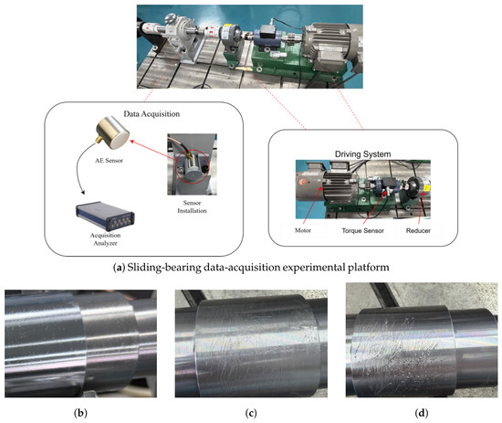
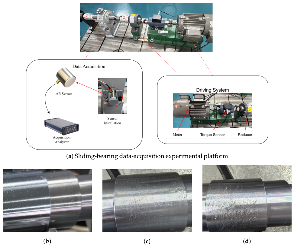
An MAE-150 AE sensor was employed to acquire signals reflecting the operating state of the sliding bearing. The AE signals were sampled at 216 kHz. The experiment was conducted under no-load conditions, and the spindle speeds were set to 60 rpm, 90 rpm, and 115 rpm. The three labels were obtained from wear conditions imposed sequentially on the same shaft. Label 0 denotes the healthy, unworn condition before artificial wear was introduced. Wear was then introduced artificially on the same shaft surface to establish the Label 1 mild-wear condition, and the wear was further aggravated to establish the Label 2 severe-wear condition. Labels 1 and 2 therefore represent sequentially aggravated stages of the same wear process rather than separately imposed lubrication regimes. A sliding-bearing data-acquisition experimental platform was designed and built, as shown in Figure 4.

Figure 4. Experimental platform and qualitative photographs of the sequential artificial-wear preparation: (a) data-acquisition platform; (b–d) shaft-surface photographs shown in chronological order.

Figure 4b–d provides a qualitative photographic record of the progressive surface changes produced during the sequential artificial-wear preparation.

The experimental platform comprises two main subsystems: a driving system and a data-acquisition system. A variable-frequency three-phase asynchronous motor provides power for the shafting system, while a torque sensor and a reducer are used to simulate the bearing operating states under different conditions. The AE sensor is mounted on the sliding-bearing housing to capture AE signals generated during bearing operation. The acquisition analyzer collects and stores the sensor output. The EMI present during data acquisition originated from the variable-frequency drive associated with the drive motor. The same motor-drive system was used for all wear conditions and rotational speeds; consequently, the acquisitions contained EMI from the same source with the same principal frequency characteristics, including a fundamental component at approximately 15 kHz and its harmonics.

The original AE signals were divided into non-overlapping fixed-length windows of 0.5 s, with each window containing 108,000 sampling points. Dataset partitioning was performed at the signal-window level. Using rotational speed as the stratification variable and a random seed of 42, the Label 0 normal windows were randomly divided at a ratio of 80% to 20%. The former 1808 windows constituted the normal training set, while the remaining 453 windows formed a held-out normal pool. This pool was further divided, using the same rotational-speed stratification and random seed, into 317 normal windows for threshold calibration and 136 normal windows for evaluation. The final evaluation set comprised these 136 normal windows together with all 802 Label 1 and 797 Label 2 windows, giving a total of 1735 evaluation windows. Abnormal windows were not used for threshold calibration. Because partitioning was performed at the signal-window level, different Label 0 windows segmented from the same original continuous acquisition record could be assigned to the training, calibration, and evaluation subsets. Run-wise or bearing-wise partitioning was not applied. The reported sample numbers represent segmented signal windows rather than numbers of physical bearing specimens or independent experimental runs.

Each original AE recording corresponds to one .sts file used in the data-processing pipeline. Recording durations were calculated from the actual file lengths at 216 kHz. The dataset composition and partition are summarized in Table 2.

Table 2. Summary of wear conditions, AE records, and dataset partition.

Label	Wear Condition	Specimen Relation	Speed (rpm)	AE Files/Duration (s)	Windows: Train/Calibration/Evaluation (Total)
Label 0	Healthy and unworn	Same shaft	60, 90, 115	9/1133.38	1808/317/136 (2261)
Label 1	Mild wear	Same shaft	60, 90, 115	3/401.45	0/0/802 (802)
Label 2	Severe wear	Same shaft	60, 90, 115	3/399.09	0/0/797 (797)
Total	—	Three sequential conditions	—	15/1933.92	1808/317/1735 (3860)

The hardware configuration used in this experiment is as follows: an Intel Core i7-11800H CPU at 2.30 GHz, 16 GB of memory, an NVIDIA GeForce RTX 3050 Ti Laptop GPU, and the Windows 11 operating system. The models were implemented in Python 3.9 using PyTorch 2.5.1. To evaluate the influence of training randomness, five independent training runs were additionally conducted using random seeds 42, 43, 44, 45, and 46 while keeping the data partition, model architecture, and training parameters unchanged. Each run consisted of 50 epochs and used the same model-selection and evaluation procedure.

The model parameter settings are shown in Table 3.

Table 3. Parameter settings.

Parameter	Value
STFT window size	1024
STFT step size	512
Asymmetric convolution kernel size	1 × 9 and 9 × 1
Number of bottleneck-layer feature channels	12
Dropout rate	0.2
Hidden-layer activation function	ReLU
Loss function	MSE
Optimizer	Adam
Learning rate	0.0001
L2 regularization penalty factor	0.0001
Maximum number of training epochs	50

3.2. Evaluation Metrics

For performance evaluation, anomalous data are treated as the positive class, whereas normal data are treated as the negative class. Table 4 presents the corresponding confusion matrix.

Table 4. Confusion matrix of evaluation metrics.

Actual Class	Predicted as Normal Data	Predicted as Anomalous Data
Actual normal data	TN	FP
Actual anomalous data	FN	TP

Using the basic variables given in Table 4, accuracy (Acc), precision (Pre), recall (Rec), and F1-Score are selected for quantitative performance evaluation [29,30].

Accuracy (Acc) represents the fraction of all samples that are correctly classified by the model and is defined as

$$\mathrm{Acc}={\displaystyle \frac{TP+TN}{TP+TN+FP+FN}},$$

(16)

Precision (Pre) denotes the fraction of samples classified as anomalous that are truly anomalous and is defined as

$$\mathrm{Pre}={\displaystyle \frac{TP}{TP+FP}},$$

(17)

Recall (Rec) represents the fraction of actual anomalous samples correctly identified by the model and is defined as

$$\mathrm{Rec}={\displaystyle \frac{TP}{TP+FN}},$$

(18)

F1-Score, defined as the harmonic mean of precision and recall, provides an overall assessment of model robustness under severe imbalance between positive and negative samples:

$$F1-\mathrm{Score}={\displaystyle \frac{2\times \mathrm{Pre}\times \mathrm{Rec}}{\mathrm{Pre}+\mathrm{Rec}}},$$

(19)

4. Results Analysis

4.1. Limitations of Single-MSE Evaluation

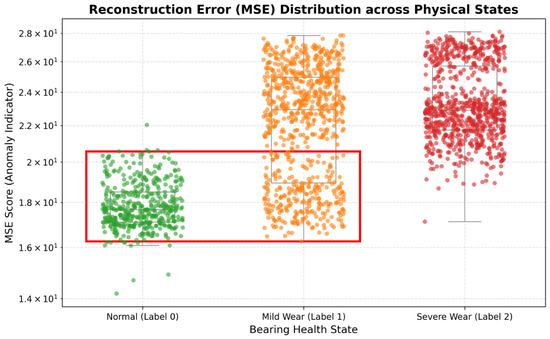
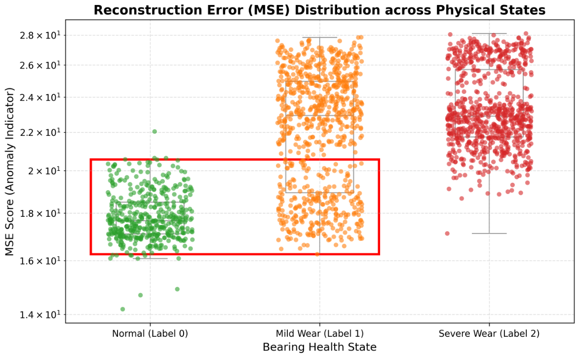
At present, most anomaly detection methods still use the reconstruction mean squared error as the main criterion for anomaly discrimination. This single indicator often has a high risk of missed detections when facing early weak anomalies. To verify the limitations of this single-evaluation system, the trained model was applied to the held-out samples to obtain one-dimensional MSE features. The data distribution results are shown in Figure 5.

Figure 5. Box-scatter distribution of single-MSE evaluation. The red rectangle indicates the overlapping region between the Label 0 and Label 1 MSE distributions.

As shown in Figure 5, Label 2 deviates from the normal baseline in terms of MSE because large-area friction causes a shift in the global energy distribution. In contrast, Label 1 is characterized by sparse and short-duration periodic transient impulses. For most of the time, its operating state is almost consistent with the normal condition of Label 0. Therefore, when calculating the global MSE, the reconstruction error caused by short-duration impulses is diluted by the dominant normal-condition components. This phenomenon, in which local weak anomalies are masked by the global averaging effect, leads to severe overlap between the MSE distributions of Label 1 and Label 0.

4.2. Analysis of the Dual-Indicator Diagnostic Plane

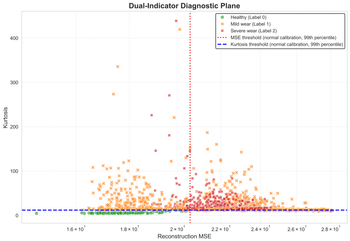
To compensate for the blind spot of the single MSE indicator in early-stage detection, this paper uses reconstruction MSE as the horizontal axis and kurtosis as the vertical axis. The final evaluation-set distribution in the resulting dual-indicator diagnostic plane is shown in Figure 6. The decision thresholds were calculated exclusively from the 317 normal calibration windows.

Figure 6. Scatter plot of the dual-indicator diagnostic plane.

Figure 6 shows that many Label 1 samples remain to the left of the MSE decision threshold because reconstruction error produced by short-duration impulses is diluted by the global averaging inherent in MSE. Their kurtosis values provide additional discrimination. For Label 2, MSE exceeds the normal baseline, while its kurtosis distribution differs from that of Label 1. The complementary responses of the two indicators across the different wear conditions provide discriminative information for anomaly detection.

Under the unified evaluation protocol, the 317 normal calibration windows were used to determine the decision thresholds, while the remaining 136 normal windows and all 1599 Label 1 and Label 2 windows were used exclusively for quantitative evaluation. To investigate sensitivity to the threshold percentile, marginal percentiles of 95%, 97.5%, 99%, and 99.5% were examined, as shown in Table 5.

Table 5. Percentile sensitivity analysis with separate threshold calibration.

q	MSE Th.	Kurtosis Th.	Cal. OR (%)	Eval. OR FPR (%)	Precision (%)	Recall (%)	F1-Score (%)
95.0%	19.9276	11.1375	7.57	7.35	99.38	99.81	99.59
97.5%	20.2906	11.7208	3.79	4.41	99.63	99.69	99.66
99.0%	20.5652	12.1146	1.89	1.47	99.87	99.37	99.62
99.5%	20.6348	12.3136	0.95	1.47	99.87	99.06	99.47

As the marginal percentile increased from 95% to 99.5%, the false-positive rate of the OR-based joint decision decreased from 7.35% to 1.47%, whereas recall decreased from 99.81% to 99.06%. At the prespecified 99th percentile, the marginal false-positive rates of MSE and kurtosis were 0% and 1.47%, respectively, and the joint false-positive rate was 1.47%. Precision, recall, and F1-score were 99.87%, 99.37%, and 99.62%, respectively. Across the investigated range, F1-score remained between 99.47% and 99.66%. Although the 97.5th percentile produced a slightly higher F1-score, the prespecified 99th percentile was retained. The 99.5th percentile, corresponding to a Bonferroni allocation of 0.5% marginal tail probability to each indicator, yielded an empirical OR-based exceedance rate of 0.95% in the calibration subset and 1.47% in the held-out normal evaluation subset.

4.3. Ablation Experiment

A series of ablation experiments were conducted to examine the contribution of each module by measuring how model performance changes after key modules are removed. An identical dataset split and hyperparameter configuration were applied to all models during training and evaluation. The designed variant models are as follows:

(1) w/o ACK: the asymmetric convolution kernel in the network is removed and replaced with a conventional standard symmetric convolution architecture.

(2) w/o Kurtosis: the kurtosis indicator is removed, and only the reconstruction MSE output by the autoencoder is used for anomaly discrimination.

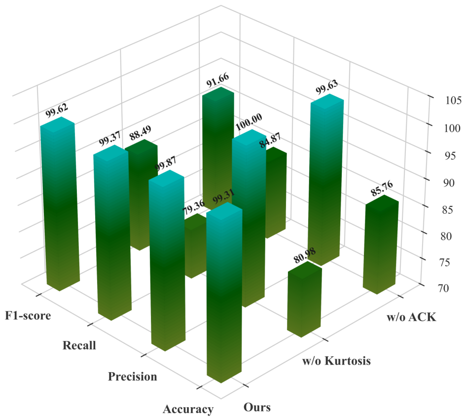
The evaluation metrics of each variant model are shown in Figure 7.

Figure 7. Evaluation results of the module ablation study.

As shown in Figure 7, the complete AADI-AD method achieved an accuracy of 99.31%, a precision of 99.87%, a recall of 99.37%, and an F1-score of 99.62%. Removing kurtosis yielded a precision of 100.00% but reduced recall to 79.36% because the decision then relied only on reconstruction MSE. Replacing the ACK module with conventional symmetric convolutions reduced recall to 84.87% and F1-score to 91.66%. These results support the contributions of the directional asymmetric-convolution module and the dual-indicator decision rule.

The roles of the 1 × 9 and 9 × 1 branches are described according to their directional receptive fields, corresponding to horizontally extended structures and vertically localized transient structures, respectively. Wu et al. [31] applied SHAP for global inspection and Grad-CAM for local temporal inspection in real-time prediction of electrochemical-machining profiles and used a physics-based model to validate unexpected events identified through anomalous model focus. A similar validation route can be applied by examining the feature contributions and attention regions of $F_{\mathrm{hor}}$ and $F_{\mathrm{ver}}$ across different samples and comparing them with the 15 kHz EMI and its harmonics, transient bearing responses, and corresponding physics-based models.

4.4. Comparative Experiment

Table 6 compares three anomaly-decision strategies using the same reconstruction output, calibration subset, evaluation set, and time-domain kurtosis. The first uses reconstruction MSE only. The second applies linear MSE–kurtosis score fusion, $S_{\mathrm{lin}}=e+\alpha \kappa$, where e is reconstruction MSE and $\kappa$ is kurtosis. The scale-balancing coefficient is $\alpha =\mathrm{mean}\left(e_0\right)/[\mathrm{mean}\left({\kappa }_0\right)+{10}^{-8}]$, where $e_0$ and ${\kappa }_0$ denote the MSE and kurtosis of the 317 normal calibration windows. These calibration windows yielded $\alpha =2.72093$, and the 99th-percentile threshold of $S_{\mathrm{lin}}$ was 53.2077. The third strategy retains separate 99th-percentile thresholds for MSE and kurtosis and applies the OR rule; the corresponding thresholds were 20.5652 and 12.1146.

Table 6. Comparison of anomaly-decision strategies using the same reconstruction output.

Decision Strategy	Accuracy (%)	Precision (%)	Recall (%)	F1-Score (%)
MSE-only decision	80.98	100.00	79.36	88.49
Linear MSE–kurtosis score fusion	96.83	99.87	96.69	98.25
MSE–kurtosis OR decision (AADI-AD)	99.31	99.87	99.37	99.62

The linear score-fusion strategy achieved a recall of 96.69% and an F1-score of 98.25%, compared with 79.36% and 88.49% for MSE-only evaluation. The MSE–kurtosis OR decision achieved a recall of 99.37% and an F1-score of 99.62%. Thus, retaining separate thresholds and combining decisions through the OR rule produced higher recall and F1-score than compressing the two indicators into one linear score.

To broaden the comparison, representative one-class machine learning and reconstruction-based methods were evaluated using the same data partition and evaluation procedure. Isolation Forest and One-Class SVM used RMS, peak value, crest factor, kurtosis, and skewness. A symmetric STFT convolutional autoencoder (CAE) used the same STFT input representation and conventional 3 × 3 convolutions, with either MSE-only or MSE–kurtosis OR decisions. A convolutional STFT variational autoencoder (VAE) was also included. The deep baselines were trained for 50 epochs using random seed 42. The results are presented in Table 7.

Table 7. Performance comparison with additional anomaly-detection methods.

Method	Accuracy (%)	Precision (%)	Recall (%)	F1-Score (%)
Isolation Forest	94.52	99.80	94.25	96.94
One-Class SVM	92.16	99.93	91.56	95.56
Symmetric STFT CAE (MSE only)	32.10	99.53	26.45	41.80
Symmetric STFT CAE (MSE + kurtosis OR)	92.28	99.73	91.87	95.64
Convolutional STFT VAE	92.22	99.66	91.87	95.61
AADI-AD	99.31	99.87	99.37	99.62

Isolation Forest, One-Class SVM, and the convolutional STFT VAE achieved F1-scores of 96.94%, 95.56%, and 95.61%, respectively. For the symmetric STFT CAE, incorporating kurtosis through the OR rule increased recall from 26.45% to 91.87% and F1-score from 41.80% to 95.64%. Under the same OR decision rule, AADI-AD achieved a recall of 99.37% and an F1-score of 99.62%, exceeding the symmetric STFT CAE.

The AADI-AD values in Table 6 and Table 7 correspond to the best-performing model retained during model development. The statistical results over five independent training runs under the same calibration and evaluation protocol are shown in Table 8. Accuracy, precision, recall, and F1-score were 99.009% ± 0.075%, 99.811% ± 0.044%, 99.112% ± 0.103%, and 99.460% ± 0.041%, respectively.

Table 8. Performance statistics over five independent training runs.

Method	Accuracy (%)	Precision (%)	Recall (%)	F1-Score (%)
AADI-AD	$99.009\pm 0.075$	$99.811\pm 0.044$	$99.112\pm 0.103$	$99.460\pm 0.041$

5. Conclusions

This paper proposes an anomaly detection model based on asymmetric convolution and a dual-indicator diagnostic plane for sliding-bearing monitoring under the EMI-contaminated conditions represented by the present experimental platform. The proposed method combines directional time–frequency feature representation with joint decision-making based on reconstruction error and kurtosis.

In the experiments, AADI-AD attained a recall of 99.37% and an F1-score of 99.62%, exceeding the corresponding values of the MSE-only decision and linear MSE–kurtosis score-fusion strategies. The ablation study supports the contributions of the asymmetric convolution kernels and the MSE–kurtosis joint decision. The two indicators provide complementary responses across the examined wear conditions and reduce missed detections compared with single-MSE evaluation.

Future research may further explore multi-scale adaptive asymmetric convolutional networks and attempt to introduce statistical methods such as extreme value theory to achieve dynamic optimization of decision boundaries, thereby providing more reliable support for predictive maintenance of rotating machinery under extremely variable operating conditions.

References

- Chang, X.; Liu, J.; Yan, X.; Sun, F.; Zhu, H.; Wang, C. Experimental Study on the Effects of Controllable Parameters on the Healthy Operation of SF-2A Material Water-Lubricated Stern Bearing in Multi-Point Ultra-Long Shaft Systems of Ships. J. Mar. Sci. Eng. 2025, 13, 14. [Google Scholar] [CrossRef] [Scilit]
- Laubichler, C.; Kiesling, C.; Marques da Silva, M.; Wimmer, A.; Hager, G. Data-Driven Sliding Bearing Temperature Model for Condition Monitoring in Internal Combustion Engines. Lubricants 2022, 10, 103. [Google Scholar] [CrossRef] [Scilit]
- Ates, C.; Höfchen, T.; Witt, M.; Koch, R.; Bauer, H.-J. Vibration-Based Wear Condition Estimation of Journal Bearings Using Convolutional Autoencoders. Sensors 2023, 23, 9212. [Google Scholar] [CrossRef] [Scilit] [PubMed]
- Chen, X.; Jiang, Y.; Zhou, B.; Zhan, H.; Li, H.; Lyu, G.; Sun, S. Early Weak Fault Diagnosis of Rolling Bearings Based on Fiber Bragg Grating Sensing Monitoring. Symmetry 2021, 13, 1473. [Google Scholar] [CrossRef] [Scilit]
- Smith, W.A.; Fan, Z.; Peng, Z.; Li, H.; Randall, R.B. Optimised spectral kurtosis for bearing diagnostics under electromagnetic interference. Mech. Syst. Signal Process. 2016, 75, 371–394. [Google Scholar] [CrossRef] [Scilit]
- Mauricio, A.; Qi, J.; Smith, W.A.; Sarazin, M.; Randall, R.B.; Janssens, K.; Gryllias, K. Bearing diagnostics under strong electromagnetic interference based on Integrated Spectral Coherence. Mech. Syst. Signal Process. 2020, 140, 106673. [Google Scholar] [CrossRef] [Scilit]
- Ling, X.; Tong, Z.; Li, O.; Wang, Z.; Xia, P.; Qin, C.; Huang, Y.; Liu, C. A novel hybrid-attention and residual mechanism-based transfer network for diesel engine small-sample misfire fault diagnosis under noise conditions. Meas. Sci. Technol. 2026, 37, 276112. [Google Scholar] [CrossRef] [Scilit]
- Tama, B.A.; Vania, M.; Lee, S.; Lim, S. Recent advances in the application of deep learning for fault diagnosis of rotating machinery using vibration signals. Artif. Intell. Rev. 2023, 56, 4667–4709. [Google Scholar] [CrossRef] [Scilit]
- Zhao, J.; Wang, W.; Huang, J.; Ma, X. A comprehensive review of deep learning-based fault diagnosis approaches for rolling bearings: Advancements and challenges. AIP Adv. 2025, 15, 020702. [Google Scholar] [CrossRef] [Scilit]
- Liu, F.T.; Ting, K.M.; Zhou, Z.-H. Isolation-based anomaly detection. ACM Trans. Knowl. Discov. Data 2012, 6, 1–39. [Google Scholar] [CrossRef] [Scilit]
- Shin, H.J.; Eom, D.H.; Kim, S.S. One-class support vector machines—An application in machine fault detection and classification. Comput. Ind. Eng. 2005, 48, 395–408. [Google Scholar] [CrossRef] [Scilit]
- Wen, L.; Li, X.; Gao, L.; Zhang, Y. A new convolutional neural network based data-driven fault diagnosis method. IEEE Trans. Ind. Electron. 2018, 65, 5990–5998. [Google Scholar] [CrossRef] [Scilit]
- Yan, X.; Xu, Y.; She, D.; Zhang, W. Reliable Fault Diagnosis of Bearings Using an Optimized Stacked Variational Denoising Auto-Encoder. Entropy 2022, 24, 36. [Google Scholar] [CrossRef] [Scilit] [PubMed]
- Shi, L.; Su, S.; Wang, W.; Gao, S.; Chu, C. Bearing Fault Diagnosis Method Based on Deep Learning and Health State Division. Appl. Sci. 2023, 13, 7424. [Google Scholar] [CrossRef] [Scilit]
- Lu, W.; Liu, J.; Lin, F. The Fault Diagnosis of Rolling Bearings Is Conducted by Employing a Dual-Branch Convolutional Capsule Neural Network. Sensors 2024, 24, 3384. [Google Scholar] [CrossRef] [Scilit] [PubMed]
- Ding, Y.; Jia, M.; Miao, Q.; Cao, Y. A novel time-frequency Transformer based on self-attention mechanism and its application in fault diagnosis of rolling bearings. Mech. Syst. Signal Process. 2022, 168, 108616. [Google Scholar] [CrossRef] [Scilit]
- Tang, X.; Xu, Z.; Wang, Z. A Novel Fault Diagnosis Method of Rolling Bearing Based on Integrated Vision Transformer Model. Sensors 2022, 22, 3878. [Google Scholar] [CrossRef] [Scilit] [PubMed]
- Li, T.; Zhao, Z.; Sun, C.; Yan, R.; Chen, X. Domain Adversarial Graph Convolutional Network for Fault Diagnosis Under Variable Working Conditions. IEEE Trans. Instrum. Meas. 2021, 70, 3515010. [Google Scholar] [CrossRef] [Scilit]
- Ragab, M.; Chen, Z.; Zhang, W.; Eldele, E.; Wu, M.; Kwoh, C.-K.; Li, X. Conditional Contrastive Domain Generalization for Fault Diagnosis. IEEE Trans. Instrum. Meas. 2022, 71, 3506912. [Google Scholar] [CrossRef] [Scilit]
- Gao, H.; Qiu, B.; Durán Barroso, R.J.; Hussain, W.; Xu, Y.; Wang, X. TSMAE: A Novel Anomaly Detection Approach for Internet of Things Time Series Data Using Memory-Augmented Autoencoder. IEEE Trans. Netw. Sci. Eng. 2023, 10, 2978–2990. [Google Scholar] [CrossRef] [Scilit]
- Huang, X.; Wen, G.; Dong, S.; Zhou, H.; Lei, Z.; Zhang, Z.; Chen, X. Memory Residual Regression Autoencoder for Bearing Fault Detection. IEEE Trans. Instrum. Meas. 2021, 70, 3515512. [Google Scholar] [CrossRef] [Scilit]
- Antoni, J. The spectral kurtosis: A useful tool for characterising non-stationary signals. Mech. Syst. Signal Process. 2006, 20, 282–307. [Google Scholar] [CrossRef] [Scilit]
- Randall, R.B.; Antoni, J. Rolling element bearing diagnostics—A tutorial. Mech. Syst. Signal Process. 2011, 25, 485–520. [Google Scholar] [CrossRef] [Scilit]
- Ni, Q.; Ji, J.C.; Halkon, B.; Feng, K.; Nandi, A.K. Physics-Informed Residual Network (PIResNet) for rolling element bearing fault diagnostics. Mech. Syst. Signal Process. 2023, 200, 110544. [Google Scholar] [CrossRef] [Scilit]
- Raissi, M.; Perdikaris, P.; Karniadakis, G.E. Physics-informed neural networks: A deep learning framework for solving forward and inverse problems involving nonlinear partial differential equations. J. Comput. Phys. 2019, 378, 686–707. [Google Scholar] [CrossRef] [Scilit]
- Wu, Y.; Sicard, B.; Gadsden, S.A. Physics-informed machine learning: A comprehensive review on applications in anomaly detection and condition monitoring. Expert Syst. Appl. 2024, 255, 124678. [Google Scholar] [CrossRef] [Scilit]
- Nikolaou, N.G.; Antoniadis, I.A. Rolling element bearing fault diagnosis using wavelet packets. NDT E Int. 2002, 35, 197–205. [Google Scholar] [CrossRef] [Scilit]
- Qiu, H.; Lee, J.; Lin, J.; Yu, G. Wavelet filter-based weak signature detection method and its application on rolling element bearing prognostics. J. Sound Vib. 2006, 289, 1066–1090. [Google Scholar] [CrossRef] [Scilit]
- Lever, J.; Krzywinski, M.; Altman, N. Classification evaluation. Nat. Methods 2016, 13, 603–604. [Google Scholar] [CrossRef] [Scilit]
- Sokolova, M.; Lapalme, G. A systematic analysis of performance measures for classification tasks. Inf. Process. Manag. 2009, 45, 427–437. [Google Scholar] [CrossRef] [Scilit]
- Wu, M.; Yao, Z.; Verbeke, M.; Karsmakers, P.; Gorissen, B.; Reynaerts, D. Data-driven models with physical interpretability for real-time cavity profile prediction in electrochemical machining processes. Eng. Appl. Artif. Intell. 2025, 160, 111807. [Google Scholar] [CrossRef] [Scilit]
Disclaimer/Publisher’s Note: The statements, opinions and data contained in all publications are solely those of the individual author(s) and contributor(s) and not of MDPI and/or the editor(s). MDPI and/or the editor(s) disclaim responsibility for any injury to people or property resulting from any ideas, methods, instructions or products referred to in the content. |
© 2026 by the authors. Licensee MDPI, Basel, Switzerland. This article is an open access article distributed under the terms and conditions of the Creative Commons Attribution (CC BY) license.