Remaining Useful Life Prediction of Turbine Engines Using Multimodal Transfer Learning

Abstract

Remaining useful life (RUL) prediction is a core technology in prognostics and health management (PHM), crucial for ensuring the safe and efficient operation of modern industrial systems. Although deep learning methods have shown potential in RUL prediction, they often face two major challenges: an insufficient generalization ability when distribution gaps exist between training data and real-world application scenarios, and the difficulty of comprehensively capturing complex equipment degradation processes with single-modal data. A key challenge in current research is how to effectively fuse multimodal data and leverage transfer learning to address RUL prediction in small-sample and cross-condition scenarios. This paper proposes an innovative deep multimodal fine-tuning regression (DMFR) framework to address these issues. First, the DMFR framework utilizes a Convolutional Neural Network (CNN) and a Transformer Network to extract distinct modal features, thereby achieving a more comprehensive understanding of data degradation patterns. Second, a fusion layer is employed to seamlessly integrate these multimodal features, extracting fused information to identify latent features, which are subsequently utilized in the predictor. Third, a two-stage training algorithm combining supervised pre-training and fine-tuning is proposed to accomplish transfer alignment from the source domain to the target domain. This paper utilized the Commercial Modular Aero-Propulsion System Simulation (C-MAPSS) turbine engine dataset publicly released by NASA to conduct comparative transfer experiments on various RUL prediction methods. The experimental results demonstrate significant performance improvements across all tasks.

1. Introduction

PHM plays a crucial role in modern industrial production, with the core objective of improving operational efficiency and ensuring equipment reliability. PHM encompasses a variety of technologies, including anomaly detection, fault diagnosis, and life prediction, which have been widely applied across multiple fields [1,2]. Among these, RUL prediction is considered an important component. By estimating the remaining service life of equipment or components, it can predict the future health status and trends of equipment, thereby helping to achieve more accurate maintenance decisions and risk management [3,4].

In recent years, machine learning has been used to address RUL prediction problems. Machine learning methods can automatically learn complex patterns and relationships from historical data, thereby significantly improving the accuracy and generalization ability of RUL prediction [5,6,7]. Although machine learning has made some progress in rule prediction, it is highly dependent on feature selection and data quality. As a result, its ability to extract meaningful features from data in real-world applications is limited, leading to less accurate predictions. Deep learning can overcome some of the limitations of machine learning by automatically learning high-level feature representations from raw data, thereby eliminating the reliance on feature engineering in traditional machine learning methods. Additionally, deep learning models can capture complex nonlinear relationships and temporal dependencies in data, thereby improving prediction accuracy and generalization capabilities [8,9,10,11].

However, in practice, due to significant differences in the working environments, operating conditions, and operating modes of different devices, traditional deep learning methods often perform poorly when there is a distribution bias between training data and actual application scenarios, making it difficult to effectively generalize to new devices or operating conditions. To address this issue, transfer learning emerges as an effective knowledge transfer method. It leverages existing knowledge from the source domain to adaptively adjust the target domain, thereby reducing reliance on large amounts of labeled data and enhancing the model’s generalization capabilities. As a result, transfer learning is increasingly being applied in the field of RUL prediction. Fan et al. [12] proposed a transfer learning method based on the consensus self-organizing model (COSMO) to improve the generalization ability of RUL prediction for turbine engines by extracting transferable features. Wang et al. [13] proposed a framework based on meta-transfer learning for the problem of bearing fault diagnosis with few samples, retaining the general features of the source domain and fine-tuning the LSTM layer to adapt to the local degradation characteristics of the target domain. Meanwhile, to overcome the limitations of recurrent neural networks in modeling long-term dependencies and in parallel computation, researchers have also explored other advanced architectures, such as the Temporal Convolutional Network (TCN). Zhang et al. [14], for instance, proposed an attention-based TCN model and successfully applied it to the RUL prediction of aero-engines. Experiments show that this method significantly improves classification accuracy in cross-condition tasks.

The above papers all deal with the same type of data. In order to capture multimodal information, comprehensively characterize device operating conditions, and enhance the expression of degradation patterns [13,14,15,16,17], this paper innovatively proposes a multimodal fine-tuning regression framework for RUL prediction. First, Transformer and CNN networks are constructed to extract features from time-series and image data, respectively, and pre-training is completed. Next, the heterogeneous data target domain is used to retrain the different modal network frameworks. Finally, the extracted multimodal features are aligned and fused to predict RUL.

The main contributions of this paper are:

(1)

An innovative model combining transfer learning and multimodal analysis has been proposed, enabling cross-domain multimodal RUL prediction even with limited data.

(2)

To better capture the degraded features of the source domain in the target domain, this study employs a supervised two-stage feature transfer method. Additionally, by integrating multidimensional and multimodal features, the model provides a more comprehensive assessment of the overall trend.

(3)

Extensive experiments were conducted, and through comparisons between multimodal and transfer learning approaches, the proposed model demonstrated the best performance.

2. Related Work

2.1. Transfer Learning in RUL

Transfer learning is a method that improves learning performance in a target domain by leveraging knowledge from a source domain, particularly when the target domain data are scarce or annotation costs are high. This method transfers model parameters, feature representations, or structural information learned from the source domain to significantly improve the learning efficiency and prediction accuracy of the target task. Depending on the transfer strategy, transfer learning methods can generally be categorized into four types: model-based methods, instance-based methods, feature-based methods, and relationship-based methods. In recent years, transfer learning has garnered significant attention in the field of RUL prediction [18,19,20,21]. Li et al. [22] proposed a segmented RUL prediction method based on multi-feature space cross-adaptive transfer learning, introducing the adaptive gradient iteration partitioning (AGIP) algorithm and the physical degradation rate-informed (PDRI) marking method, which effectively alleviates the problem of data distribution differences. Cao et al. [23] proposed a bearing remaining life prediction method (TBIGRU) based on bidirectional GRU and transfer learning, combining DTW and Wasserstein distance to screen features and designing adaptive condition identification indicators. Experiments showed that the prediction error was significantly reduced and the cross-condition performance was superior to traditional transfer learning methods.

This study focuses on the key challenges of transfer learning in data-driven RUL prediction, namely, how to effectively transfer model parameters learned from related source domains (data-rich) to RUL prediction tasks in target domains (data-scarce). The core feature of parameter transfer schemes is to pre-train models using a large amount of source domain data and then fine-tune them to adapt to a small amount of target domain labeled data. The advantages of this method are: (1) it avoids training models from scratch, significantly saving computational resources; (2) it utilizes the general feature representations of the source domain to alleviate the overfitting problem caused by insufficient target domain data. Although existing research has made some progress in RUL prediction, there are still obvious limitations: existing methods are mostly based on single-modality data (such as vibration signals or temperature data) and fail to fully utilize multimodal data (such as acoustic emission, current signals, and other multi-source information) to comprehensively characterize the equipment degradation process. Multimodal data provide richer information about equipment status, and by fusing features from different modalities, they are expected to further improve the accuracy and robustness of RUL prediction.

2.2. Multimodal Method

Multimodal refers to data from multiple sources that are semantically related and may contain complementary information, such as images, speech, time-domain and frequency-domain signals, and natural language text. Multimodal learning aims to build models capable of processing and integrating different data modalities to obtain more comprehensive information. In the field of PHM, multimodal methods typically refer to the integration of data from multiple sensors, data sources, or different physical measurement methods to improve the accuracy of equipment anomaly detection, fault diagnosis, and RUL prediction. By integrating complementary information from different modalities, models can more accurately understand the operating status and degradation trends of equipment.

Currently, multimodal methods have achieved significant results in multiple fields. For example, Razzaghi et al. [24] proposed a model based on multimodal deep transfer learning, which utilizes multimodal feature encoders and domain adaptation techniques to leverage multimodal medical imaging (MRI) data, significantly improving the performance of brain tumor detection and segmentation tasks. Rahman et al. [25] developed a multimodal adaptation gate (MAG) that enables pre-trained Transformer models (such as BERT and XLNet) to fuse non-linguistic data such as visual and audio data, thereby demonstrating a superior performance in multimodal sentiment analysis tasks. In the field of PHM, Ji et al. [26] proposed a supervised variational autoencoder (SVAE) that achieves efficient anomaly detection and fault diagnosis by integrating high-dimensional LiDAR data and low-dimensional encoder data. SVAE unifies the optimization objectives of generative and discriminative models, simplifies the training process, and demonstrates multimodal classification capabilities superior to baseline methods on a farm robot dataset.

However, existing research in the field of PHM has mainly focused on the fusion of temporal multimodal data, while multimodal methods remain largely unexplored in the field of RUL prediction. Traditional methods typically only utilize temporal data from different dimensions for fusion, resulting in single-feature and incomplete information. To address this issue, this paper proposes a multimodal method that combines image and temporal data to more comprehensively capture the degradation characteristics of equipment, thereby improving the accuracy and robustness of RUL prediction.

3. Method

3.1. Overview

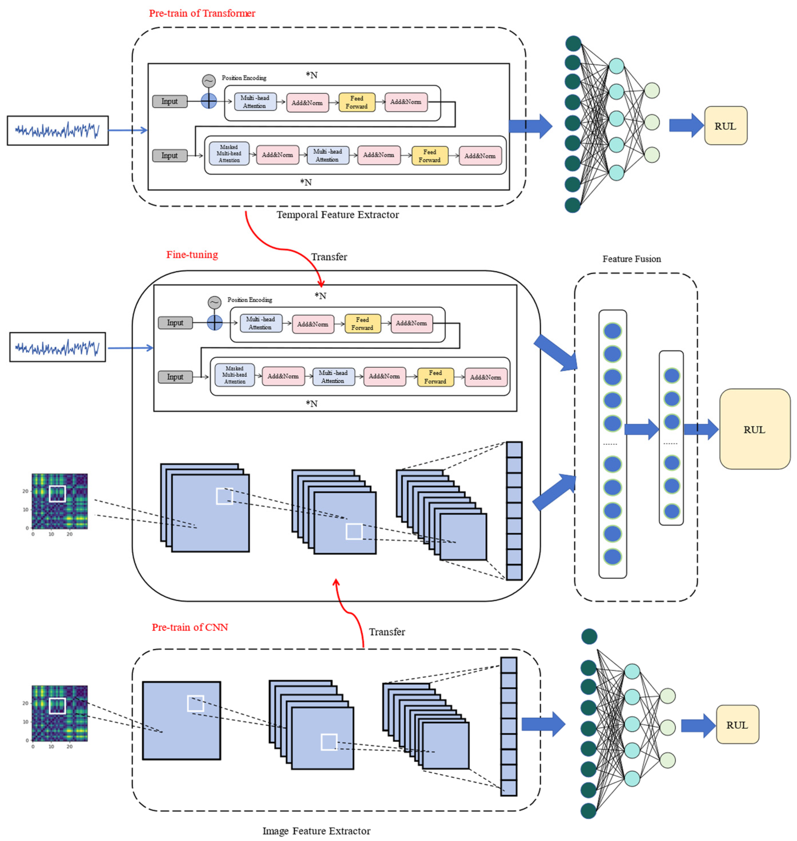
To comprehensively characterize the degradation trend of equipment and accurately predict its RUL, this paper proposes a regression framework based on multimodal fine-tuning transfer learning. This framework integrates time-series signals and image data to construct a cross-modal feature collaboration mechanism, thereby comprehensively capturing the dynamic characteristics of equipment degradation from heterogeneous data.

The model adopts a multimodal pre-training strategy: first, a Transformer network is used to extract deep time–frequency features from time-series data, while a CNN architecture is employed to learn spatial degradation representations from image data, and preliminary RUL prediction modeling is completed in the source domain. Subsequently, a two-stage transfer learning mechanism is employed to enhance the model’s generalization ability: during the fine-tuning phase in the target domain, the heterogeneous features extracted from the time-series and image modalities are adaptively aligned and deeply fused in the shared hidden layers, leveraging cross-modal complementary information to optimize feature representation. This transfer strategy not only addresses the distribution differences between heterogeneous data but also significantly improves the model’s RUL prediction accuracy under unknown operating conditions through domain adaptation learning.

3.2. Multimodal Data Input

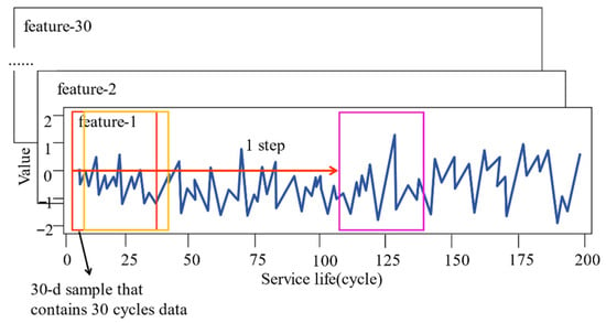
In the C-MAPSS dataset, each single-cycle sample consists of a 30-dimensional feature vector, including 3 operational parameters, 21 sensor measurements, and 6 unique heat encoding features. As shown in Figure 1, we use a sliding window method to sample the multivariate time series. As shown in Figure 2, the window length is set to 30 time steps, a value commonly adopted in the C-MAPSS literature that balances capturing a sufficient degradation pattern with computational efficiency. The sliding step is set to 1, and the model input samples are generated sequentially. The true RUL value corresponding to each sample is determined by the RUL of the last single-cycle sample within its window. In terms of data partitioning, 20% of the trajectories in the training set are randomly selected as the validation set; the test set uses the last sliding window of each trajectory as the input sample.

Figure 1. Regression framework diagram for multimodal fine-tuning transfer learning.

Figure 2. Extracting time-series samples from input.

To fully explore the multimodal characteristics of time-series data, recurrence plots (RPs) are introduced as input representations for image modalities. RP is a visualization tool that can effectively reveal repetitive patterns and dynamic system characteristics in time series. Its core principle is to construct a graphical representation of state repetitions in a two-dimensional plane by calculating the similarity between time-series points [27]. When the distance between the states at two time points is less than a predefined threshold, mark the corresponding points in the RP diagram to ultimately form an image with specific texture features. In this experiment, the 30-dimensional feature vector is converted into a 30 × 30 RP diagram, which serves as the visual modality input for the CNN network.

By combining the original time-series data and RP images as dual-modal input, the DMFR model can analyze temporal features from different perspectives: the Transformer network directly processes the original time-series signals to capture their temporal dynamic characteristics; the CNN network extracts spatial texture features from the RP images to reveal periodic patterns and state transition rules in the sequence. This multimodal fusion strategy significantly enhances the model’s ability to comprehensively characterize device degradation features.

3.3. RUL Prediction Model

3.3.1. Image Feature Extractor

The image feature extractor designed in this paper aims to capture the correlation patterns in time-series data by converting time-series data into RP and extracting their features. The feature extractor adopts a CNN architecture. Specifically, a CNN architecture comprises 4 convolutional layers with filter counts of [16, 32, 64, 128], respectively, designed to extract hierarchical features from the RP images. Each convolutional layer is followed by a ReLU activation and a 2 × 2 max-pooling layer, and the specific processing flow is as follows:

Let the input RP diagram be the feature matrix, where H = W = 30 denotes the dimensions of the RP diagram. First, perform a convolution operation on the RP diagram to extract local features using a sliding convolution kernel. The convolution operation can be expressed as:

$$\begin{array}{c}{\mathrm{X}}_1\left(i,j\right)={\displaystyle \sum _a}{\displaystyle {\sum }_b}\mathrm{Z}\left(i+a,j+b\right)·\omega \left(a,b\right)+c\end{array}$$

(1)

Among them, $\mathsf{\omega }\in {\mathrm{R}}^{\mathrm{k}\times \mathrm{k}}$ is the convolution kernel weight, $\mathrm{c}$ is the bias term, $\mathsf{\sigma }(·)$ represents the activation function, and ${\mathrm{X}}_1$ is the output feature map. Subsequently, maximum pooling is performed on the feature map to reduce the feature dimension and retain significant features:

$${\mathrm{Y}}_1\left(\mathrm{i},\mathrm{j}\right)=\max {{\mathrm{X}}_1}_{\mathrm{pi}}\left(\mathrm{i}+\mathrm{p},\mathrm{j}+\mathrm{q}\right)$$

(2)

Among them, ${{\mathrm{X}}_1}_{\mathrm{pi}}\left(\mathrm{i}+\mathrm{p},\mathrm{j}+\mathrm{q}\right)$ is the pixel value at the position $\left(\mathrm{i}+\mathrm{p},\mathrm{j}+\mathrm{q}\right)$ in the input feature map. $\mathrm{p},\mathrm{q}$ are the relative offsets within the pooling window. ${\mathrm{Y}}_1\left(\mathrm{i},\mathrm{j}\right)$ represents the pixel value in the output feature map after pooling. The extracted feature is ${\mathrm{V}}_1$:

$${\mathrm{V}}_1=\mathrm{CNN}\left(\mathrm{Z}\right)$$

(3)

In the formula, ${\mathrm{V}}_1$ is the deep feature representation extracted by CNN. This feature will be fused with the temporal features to improve the model’s ability to express device degradation features.

3.3.2. Time-Series Feature Extractor

When extracting time-series features, this network is based on the Transformer structure to build a device performance evaluation framework with it as the main network.

The temporal feature extractor constructed in this paper adopts the Transformer framework, which includes N encoders and decoders of the same number. The Transformer consists of 4 encoder layers with 8 attention heads each, a configuration chosen to balance the model’s capacity to capture complex temporal dependencies against the risk of overfitting.

Assuming that the feature matrix of the model input is M, the feature matrix with added position information is first obtained through the position encoding layer:

$${\mathrm{M}}_{\mathrm{Q}}=\mathrm{POS}\left(\mathrm{M}\right)$$

(4)

The encoded ${\mathrm{M}}_{\mathrm{Q}}$ is input into a temporal feature extractor constructed using Transformer, and then processed by an encoder and decoder to extract high-level features, thereby achieving temporal modeling of the input data. The formula is expressed as follows:

$$\begin{array}{c}{\mathrm{M}}_{\mathrm{Er}}={\mathrm{Er}}_{\mathrm{N}}\left({\dots \mathrm{Er}}_2\left({\mathrm{Er}}_1\left({\mathrm{M}}_{\mathrm{Q}}\right)\right)\right)\end{array}$$

(5)

$${\mathrm{M}}_{\mathrm{Dr}}={\mathrm{Dr}}_{\mathrm{nnN}}\left({\dots \mathrm{Dr}}_2\left({\mathrm{Dr}}_1\left({\mathrm{M}}_{\mathrm{Er}},{\mathrm{M}}_{\mathrm{Q}}\right)\right)\right)$$

(6)

In this equation, ${\mathrm{Er}}_{\mathrm{i}}$ denotes the i-th encoder block, ${\mathrm{D}\mathrm{r}}_{\mathrm{i}}$ denotes the i-th decoder block, ${\mathrm{M}}_{\mathrm{Er}}$ denotes the output of the encoder part, and ${\mathrm{M}}_{\mathrm{Dr}}$ denotes the output of the decoder part. The extracted feature is ${\mathrm{V}}_2$:

$${\mathrm{V}}_2=\mathrm{Transformer}\left({\mathrm{M}}_{\mathrm{Q}}\right)$$

(7)

In this equation, ${\mathrm{V}}_2$ represents the feature matrix extracted after processing using Transformer.

3.3.3. Fusion Prediction

When processing the image data, convolutional and pooling operations of image feature extractors are used to obtain image features. Let the output dimension of the CNN fully connected layer be ${\mathrm{N}}_1$, and the extracted image features can be represented as ${\mathrm{V}}_1\in {\mathrm{R}}^{{\mathrm{N}}_1}$.

When processing homogeneous time-series data, a time-series feature extractor is used, and the dimension of the final output layer of the Transformer encoder is set to ${\mathrm{N}}_2$. The extracted time-series features are denoted as ${\mathrm{V}}_2\in {\mathrm{R}}^{{\mathrm{N}}_2}$.

In the feature fusion and regression prediction stage, a fusion layer and a RUL predictor were designed. The fusion layer consists of two fully connected structures, with the first layer and second layer containing ${\mathrm{N}}_{\mathrm{F}1}$ and ${\mathrm{N}}_{\mathrm{F}2}$ neurons, respectively. The output of the CNN fully connected layer is concatenated with the output of the Transformer encoding layer, and the first fully connected operation is used to achieve the preliminary integration of multimodal features. Then, the second nonlinear transformation generates a unified feature vector ${\mathrm{V}}_{\mathrm{in}}$, and the calculation formula is as follows:

$${\mathrm{V}}_{\mathrm{in}}=\mathsf{\sigma }\left({\mathrm{W}}_{\mathrm{F}2}\mathsf{\sigma }\left({\mathrm{W}}_{\mathrm{F}1}\left[{\mathrm{V}}_{\mathrm{C}};{\mathrm{V}}_{\mathrm{T}}\right]+{\mathrm{b}}_{\mathrm{F}1}\right)+{\mathrm{b}}_{\mathrm{F}2}\right)$$

(8)

In this equation, $\left[{\mathrm{V}}_{\mathrm{C}};{\mathrm{V}}_{\mathrm{T}}\right]$ represents the feature concatenation operation, ${\mathrm{W}}_{\mathrm{F}1}$, ${\mathrm{W}}_{\mathrm{F}2}$, ${\mathrm{b}}_{\mathrm{F}1},{\mathrm{b}}_{\mathrm{F}2}$ represent the weights and biases of each layer, respectively, and $\mathsf{\sigma }$ represents the activation function.

Finally, the merged feature vector ${\mathrm{V}}_{\mathrm{in}}$ is input into the regression layer for RUL prediction. The prediction process is as follows:

$$\widehat{\mathrm{y}}={\mathrm{W}}_{\mathrm{reg}}\cdot {\mathrm{V}}_{\mathrm{in}}+{\mathrm{b}}_{\mathrm{reg}}$$

(9)

where $\widehat{\mathrm{y}}$ is the predicted remaining useful life of the equipment, and ${\mathrm{W}}_{\mathrm{reg}}$ and ${\mathrm{b}}_{\mathrm{reg}}$ are the regression layer parameters. The model optimization uses the MSE loss function to improve the prediction accuracy by minimizing the Euclidean distance deviation between the predicted values and the actual values.

3.4. Two-Stage Transfer Strategy

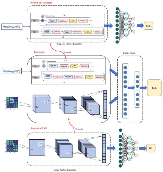
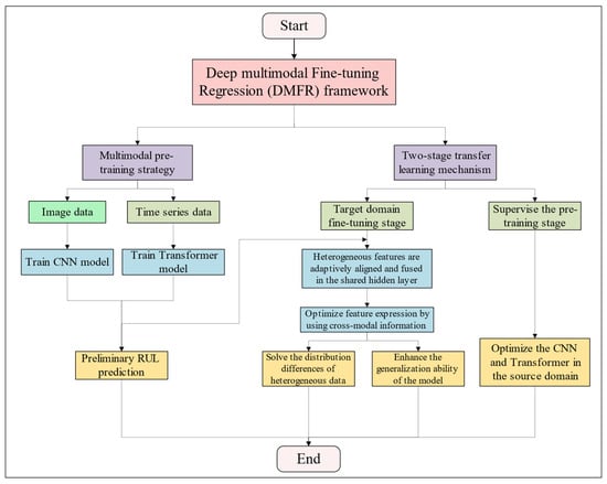
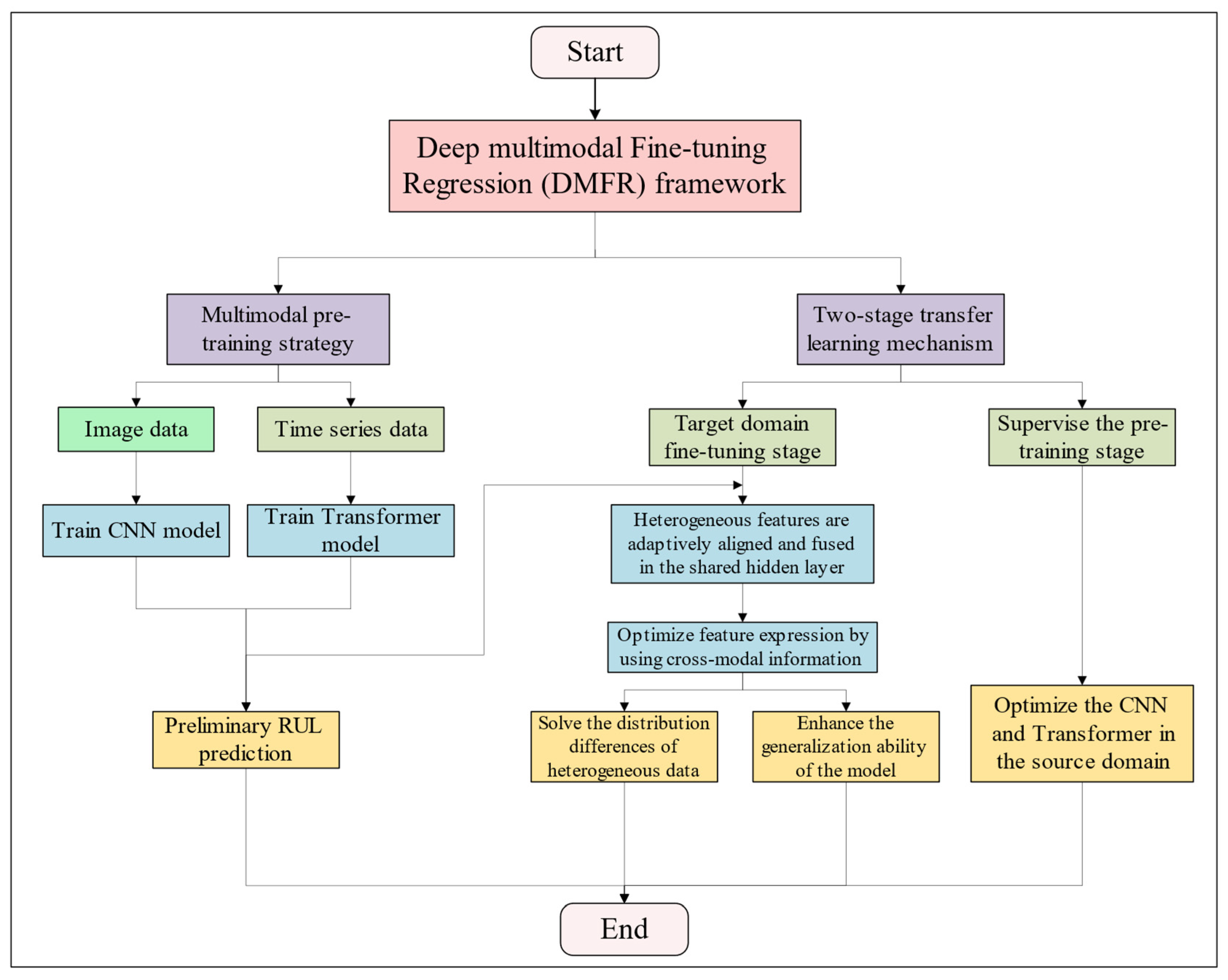
To address the challenge of adapting heterogeneous modal data in cross-domain scenarios, this paper innovatively proposes a multimodal fusion framework based on two-stage transfer learning. By combining supervised pre-training and fine-tuning, the framework comprehensively characterizes the device degradation features. Figure 3 shows the flowchart of the two-stage transfer framework DMFR for heterogeneous modal data.

Figure 3. Two-stage transfer framework DMFR flowchart.

The core of this framework lies in constructing a time-series—image dual-branch feature extraction network, where the Transformer branch focuses on extracting deep temporal–frequency domain features from temporal signals, while the CNN branch effectively captures spatial degradation patterns in RP images. During the supervised pre-training phase, the two branches are trained independently on the source domain data: for the CNN image branch, after initializing the network parameters, forward propagation is performed, and the network parameters are optimized by minimizing the cross-entropy loss function, as shown below:

$$\mathrm{C}=-\sum _{\mathrm{k}}1\left({\mathrm{z}}_{\mathrm{k}}\right)\log \left({\mathrm{a}}_{\mathrm{k}}\right)$$

(10)

In this equation, $1\left({\mathrm{z}}_{\mathrm{k}}\right)$ is an indicator function that is 1 if ${\mathrm{z}}_{\mathrm{k}}$ is true and 0 otherwise. ${\mathrm{a}}_{\mathrm{k}}$ and ${\mathrm{z}}_{\mathrm{k}}$ are the output and label of the k-th neuron in the classification layer, respectively.

For the Transformer temporal branching, training is performed based on the calculation rules in the previous section.

For these two models, the update process for each parameter during BP can be expressed using the chain rule as follows:

$$\mathsf{\delta }={\displaystyle \frac{\partial \mathrm{C}}{\partial \mathrm{b}}}={\displaystyle \frac{\partial \mathrm{C}}{\partial \mathrm{a}}}{\displaystyle \frac{\partial \mathrm{a}}{\partial \mathrm{Z}}}{\displaystyle \frac{\partial \mathrm{Z}}{\partial \mathrm{b}}}$$

(11)

$${\displaystyle \frac{\partial {\mathrm{a}}_{\mathrm{j}}}{\partial {\mathrm{Z}}_{\mathrm{j}}}}=\left\{\begin{array}{llll}{\mathrm{a}}_{\mathrm{j}}\left(1-{\mathrm{a}}_{\mathrm{j}}\right),& & & \mathrm{if}\mathrm{j}=\mathrm{i}\\ -{\mathrm{a}}_{\mathrm{j}}{\mathrm{a}}_{\mathrm{i}},& \hspace{1em}\mathrm{otherwise}& & \end{array}\right.$$

(12)

$$\mathsf{\Delta }{\mathrm{W}}^{\mathrm{l}}=-\mathsf{\eta }{\displaystyle \frac{\partial \mathrm{C}}{\partial {\mathrm{W}}^{\mathrm{l}}}}=-\mathsf{\eta }{\mathrm{a}}^{\mathrm{l}-1}{\left(\left({\mathsf{\delta }}^{\mathrm{l}}\right)\right)}^{\mathrm{T}}{\mathrm{W}}^{\mathrm{l}}={\mathrm{W}}^{\mathrm{l}}+\mathsf{\Delta }{\mathrm{W}}^{\mathrm{l}}$$

(13)

In this equation, ${\mathrm{Z}}_{\mathrm{j}}$ is the input of the j-th neuron, ${\mathrm{a}}_{\mathrm{j}}$ is the output of the j-th neuron, ${\mathsf{\Delta }\mathrm{W}}^{\mathrm{l}}$ is the weight increment of layer $\mathrm{l}$, and $\mathsf{\eta }$ is the learning rate. Repeat the iteration until the accuracy of both models reaches their respective thresholds.

In the model fine-tuning stage, the feature fusion layer and RUL prediction layer are first randomly initialized, and the cross-modal features extracted from pre-training are used as the input for the preliminary training. Subsequently, the pre-trained model is structurally modified: the original output layer of the Transformer branch is removed, and its encoder module is retained as a temporal feature extractor; the CNN branch is processed synchronously, and after removing the classification layer, its convolution module is transferred to the fusion network. The modified dual-branch network and the preliminarily trained feature fusion layer together constitute the complete prediction framework. In the specific implementation process, to ensure the temporal synchrony of multimodal data, uniform timestamp annotations are applied to the original time-series signals and the image data are converted using RP. Finally, an end-to-end supervised learning strategy is adopted to jointly optimize all network parameters, including CNN convolution kernel weights, Transformer encoder parameters, and fusion layer weights, based on the backpropagation algorithm, thereby significantly improving the model’s generalization ability in the target domain. The experimental results demonstrate that this transfer learning framework can effectively overcome the differences in heterogeneous data distributions and achieve accurate characterization of device degradation trajectories through cross-modal feature complementarity mechanisms.

4. Experiment

4.1. Dataset Description

The C-MAPSS is an aviation engine simulation dataset that was released by NASA in 2008, commonly used in the field of remaining life prediction.

Specifically, the C-MAPSS model simulates a high-bypass ratio turbofan engine, which is a realistic representation of a modern commercial aircraft engine. The model includes several key rotating components, such as the fan, low-pressure compressor (LPC), high-pressure compressor (HPC), high-pressure turbine (HPT), and low-pressure turbine (LPT). The different fault modes within the dataset are generated by simulating the performance degradation of one or more of these core components, providing valuable data for studying the evolution of an engine from a healthy state to final failure.

The C-MAPSS dataset consists of four subsets: FD001, FD002, FD003, and FD004, where “FD” is an abbreviation for “Fault Data”. Each subset in the C-MAPSS dataset comprises a training set and a test set, with each record providing detailed information about engine performance and degradation. The primary distinction between these subsets lies in the complexity of their Operating Conditions (OCs) and Fault Modes (FMs), with the specifics summarized in Table 1.

Table 1. Information about the C-MAPSS dataset.

Data	FD001	FD002	FD003	FD004
Train	100	260	100	249
Test	100	259	100	248
OC	1	6	1	6
FM	1	1	2	2

OC defines the number of operational conditions that the engine undergoes. OC = 1 (used in FD001 and FD003) signifies that the engine operates under a single, constant condition. In contrast, OC = 6 (used in FD002 and FD004) indicates that the engine operates under six different and more complex conditions, simulating a more realistic flight profile.

FM defines the types of simulated faults that lead to engine failure. FM = 1 (used in FD001 and FD002) represents a single fault mode, which is the degradation of the HPC. FM = 2 (used in FD003 and FD004) involves two concurrent fault modes: degradation of both the HPC and the fan.

The engines represented in the C-MAPSS dataset exhibit varying degrees of initial wear; however, at the start of each record, they are considered to be in a healthy state. Over time, as the number of operating cycles increases, the engines gradually degrade until they reach a point where they can no longer operate effectively, at which stage they are classified as unhealthy. The training dataset captures the complete lifecycle of each engine, from its initial healthy state to its final failure. In contrast, the test dataset consists of time-series data that end at a specific point prior to system failure. The primary objective associated with this dataset is to predict the RUL of engines in the test set. RUL refers to the time or number of operating cycles that a system, component, or machine is expected to continue operating within acceptable performance limits before failure or maintenance is required.

4.2. Dataset Preprocessing

In the study on remaining useful life prediction based on the C-MAPSS dataset, the original sensor data included monitoring signals from 21 channels. Based on previous experience [28,29,30], this study screened out 14 sensor channels with the highest discriminative ability (sensors 2, 3, 4, 7, 8, 9, 11, 12, 13, 14, 15, 17, 20, and 21) as model inputs by calculating the correlation coefficients between each sensor signal and the equipment degradation state. These selected sensors effectively capture the performance degradation characteristics of the equipment’s critical components, providing high-quality feature representations for subsequent modeling.

To address the issue of dimensional differences among multichannel sensor signals, the study employs a minimum–maximum normalization method for data preprocessing, as shown below.

$${\widehat{\mathrm{x}}}_{\mathrm{t},\mathrm{s}}={\displaystyle \frac{{\mathrm{x}}_{\mathrm{t},\mathrm{s}}-\min \left({\mathrm{x}}_{\mathrm{s}}\right)}{\max \left({\mathrm{x}}_{\mathrm{s}}\right)-\min \left({\mathrm{x}}_{\mathrm{s}}\right)}}$$

(14)

In this equation, $x_{t,s}$ is the raw measurement value of sensor $\mathrm{s}$ at time step $\mathrm{t}$. $\min \left({\mathrm{x}}_{\mathrm{s}}\right)$ is the minimum value of sensor $\mathrm{s}$ at all time steps, and $\max \left({\mathrm{x}}_{\mathrm{s}}\right)$ is the maximum value of sensor $s$ at all time steps.

At the same time, to better utilize the time information of the data, the input data are a continuous sequence of records captured within a time window of size $14\times {\mathrm{T}}_{\mathrm{w}}$. Based on prior knowledge, the turbine engine is in a healthy state during the initial operation phase and begins to deteriorate after a period of time. Therefore, the remaining life is defined as a segmented linear RUL, as shown below:

$$\mathrm{RUL}=\left({\displaystyle \genfrac{}{}{0pt}{}{\mathrm{RUL},\cdots \mathrm{if}\mathrm{RUL}\le {\mathrm{R}}_{\mathrm{early}}}{{\mathrm{R}}_{\mathrm{early}},\cdots \mathrm{if}\mathrm{RUL}>{\mathrm{R}}_{\mathrm{early}}}}\right)$$

(15)

In this equation, ${\mathrm{R}}_{\mathrm{early}}$ is the dividing point between the healthy stage and the degenerative stage. Select ${\mathrm{R}}_{\mathrm{early}}$ as a constant value and set it to 125 cycles, consistent with prior foundational studies on this dataset, as it represents an empirically observed point where significant degradation typically begins.

4.3. Evaluation Criteria

To comprehensively evaluate the performance of the RUL prediction model, this study uses four key indicators for quantitative analysis: root mean square error (RMSE), mean absolute error (MAE), coefficient of determination (R²), and score.

The definitions and calculation formulas for each indicator are as follows:

RMSE measures the magnitude of prediction errors. Its squaring of errors makes it particularly sensitive to large deviations, which is crucial for penalizing high-risk mispredictions in RUL estimation. The formula is:

$$\mathrm{RMSE}=\sqrt{\left(1/\mathrm{n}\right)\sum {\left({\mathrm{y}}_{\mathrm{i}}-{\widehat{\mathrm{y}}}_{\mathrm{i}}\right)}^2}$$

(16)

MAE offers a direct and intuitive measure of the average error size in operating cycles, reflecting the model’s typical prediction accuracy. The formula is:

$$\mathrm{MAE}=\left({\displaystyle \frac{1}{\mathrm{n}}}\right)\sum \left|{\mathrm{y}}_{\mathrm{i}}-{\widehat{\mathrm{y}}}_{\mathrm{i}}\right|$$

(17)

R² assesses the model’s goodness-of-fit by quantifying how well the predictions capture the trend of the actual RUL degradation. An R² value close to 1 indicates a high correlation with the true degradation path. The formula is:

$${\mathrm{R}}^2=1-\left(\sum {\left({\mathrm{y}}_{\mathrm{i}}-{\widehat{\mathrm{y}}}_{\mathrm{i}}\right)}^2\right)/\left(\sum {\left({\mathrm{y}}_{\mathrm{i}}-\overline{\mathrm{y}}\right)}^2\right)$$

(18)

The scoring function is an asymmetric metric specifically designed for the C-MAPSS dataset, which penalizes late predictions more heavily than early ones. The formula is:

$$\mathrm{Score}=\left\{\begin{array}{c}{\displaystyle \sum _{\mathrm{n}=1}^{\mathrm{N}}}\left({\mathrm{e}}^{-\left({\displaystyle \frac{{\mathrm{d}}_{\mathrm{n}}}{13}}\right)}-1\right),{\mathrm{d}}_{\mathrm{n}}<0\\ {\displaystyle \sum _{\mathrm{n}=1}^{\mathrm{N}}}\left({\mathrm{e}}^{\left({\displaystyle \frac{{\mathrm{d}}_{\mathrm{n}}}{10}}\right)}-1\right),{\mathrm{d}}_{\mathrm{n}}\ge 0\end{array}\right.$$

(19)

Among them, ${\mathrm{d}}_{\mathrm{n}}=\widehat{{\mathrm{y}}_{\mathrm{n}}}-{\mathrm{y}}_{\mathrm{n}}$. ${\mathrm{y}}_{\mathrm{n}}$ is the actual value, and $\widehat{{\mathrm{y}}_{\mathrm{n}}}$ is the estimated value.

These four evaluation metrics comprehensively assess the model performance from different dimensions: RMSE focuses on penalizing large errors; MAE provides an intuitive measure of error; and R² reflects the model’s ability to capture data patterns. Score is a common evaluation metric in the RUL prediction field and facilitates comparison with other methods. Through the comprehensive consideration of these three metrics, the accuracy and reliability of RUL prediction models can be evaluated more comprehensively.

4.4. Task Classification

In order to comprehensively analyze the generalization ability of this model, various transfer learning tasks were defined by combining datasets with different operating conditions and fault modes. These tasks include training on one or more datasets and testing on another dataset, as shown in Table 2.

Table 2. Transfer learning task table.

Task	Condition	OC	FM
1	FD001—FD002	1 → 6	1 → 1
2	FD001—FD003	1 → 1	1 → 2
3	FD001—FD004	1 → 6	1 → 2
4	FD002—FD001	6 → 1	1 → 1
5	FD002—FD003	6 → 1	1 → 2
6	FD002—FD004	6 → 6	1 → 2
7	FD003—FD001	1 → 1	2 → 1
8	FD003—FD002	1 → 6	2 → 1
9	FD003—FD004	1 → 6	2 → 2
10	FD004—FD001	6 → 1	2 → 1
11	FD004—FD002	6 → 6	2 → 1
12	FD004—FD003	6 → 1	2 → 2

4.5. Experimental Results and Analysis

4.5.1. RUL Prediction Results

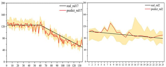
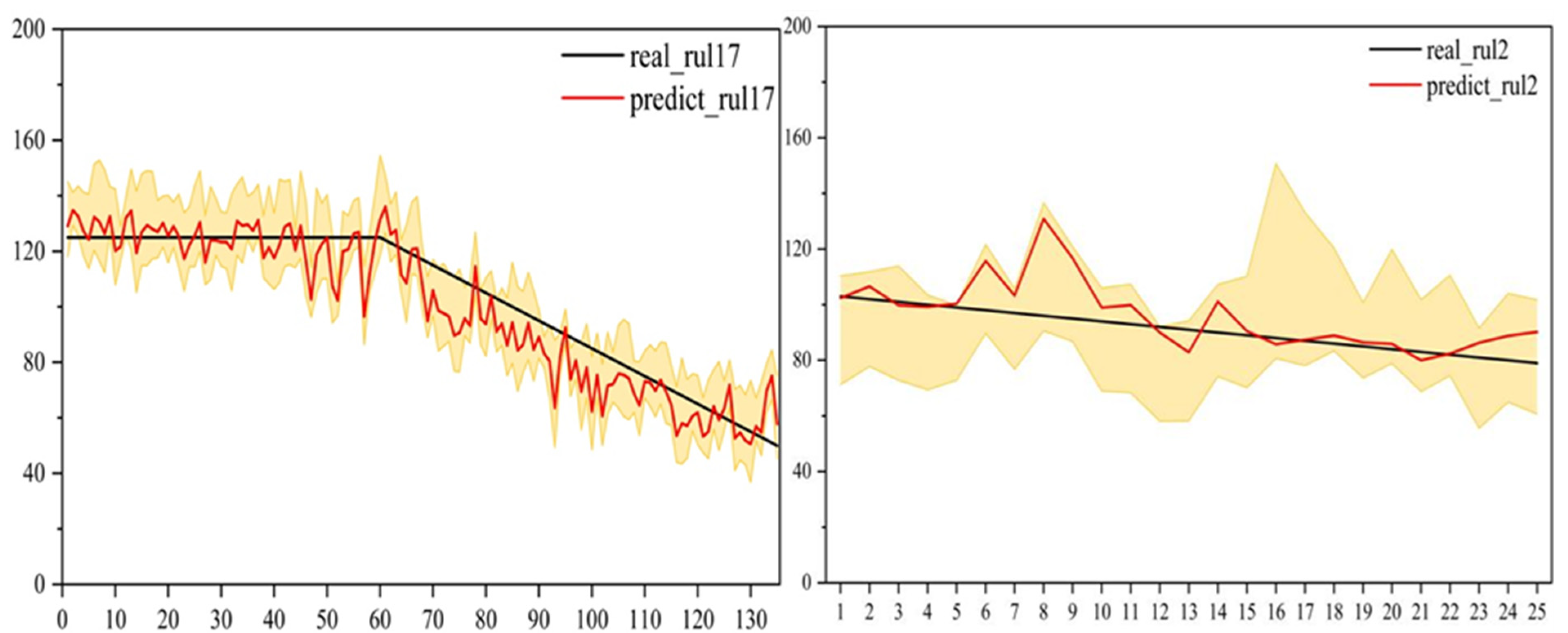
This study validated the model performance through four cross-domain transfer experiments, dividing the target domain test data into validation and test sets at a ratio of 50–50%. The trained deep network model was used to predict the RUL of unknown samples in the target domain test set. The experimental results are presented as follows: Table 3 shows the error distribution between the predicted and actual RUL values in the last time window of the test set, reflecting the model’s prediction accuracy at the end of the device’s lifespan. Figure 4 further shows the comparison between the degradation curves of typical single devices (unit 17 of task A and unit 76 of task C) throughout their entire lifecycle and the prediction results. The black solid line represents the actual RUL values, the red solid line represents the model’s predicted values, and the orange-colored shaded area represents the 95% confidence interval calculated based on multiple prediction results, effectively reflecting the stability of the prediction results.

Table 3. Prediction error for different tasks.

Criteria	RMSE	MAE	R2	Score
Task1	31.4 ± 3.1	28.6 ± 1.8	0.88 ± 0.1	3398 ± 2896
Task2	25.4 ± 42	26.3 ± 3.1	0.79 ± 0.2	3485 ± 2536
Task3	39.3 ± 2.3	29.6 ± 2.1	0.81 ± 0.1	6490 ± 3442
Task4	46.6 ± 6.2	39.5 ± 4.5	0.69 ± 0.3	58,782 ± 50,289
Task5	43.9 ± 1.3	38.7 ± 2.3	0.71 ± 0.1	51,831 ± 48,971
Task6	23.1 ± 3.0	26.9 ± 2.2	0.80 ± 0.1	3025 ± 2054
Task7	36.3 ± 2.5	33.9 ± 1.0	0.76 ± 0.2	10,598 ± 15,321
Task8	39.1 ± 4.1	38.7 ± 1.3	0.78 ± 0.3	9712 ± 5891
Task9	39.0 ± 0.7	36.9 ± 1.4	0.80 ± 0.1	8639 ± 5412
Task10	46.1 ± 2.1	42.3 ± 1.9	0.68 ± 1.0	25,909 ± 12,489
Task11	34.0 ± 2.2	33.7 ± 2.1	0.75 ± 0.3	19,578 ± 13,247
Task12	47.9 ± 1.0	46.3 ± 5.0	0.62 ± 0.2	2851 ± 17,845

Figure 4. Full lifecycle RUL prediction results for multiple engine units under different tasks.

The reported RMSE, MAE, R2, and Score values for each task are calculated based on the final RUL prediction for each engine in the test set, not across the entire degradation trajectory. The unit for these errors is “operating cycles”. The primary purpose of these results is to establish a performance baseline, which demonstrates the relative superiority of our model when compared with other methods in the subsequent sections.

The results in Table 3 indicate that the proposed method can provide predictions close to the actual values for the final recorded cycle of different target task test sets, which is crucial for maintenance guidance when faults are imminent. In addition, the results in Figure 4 show that the DMFR model has good prediction accuracy and stability.

4.5.2. Comparative Analysis with Benchmark Models

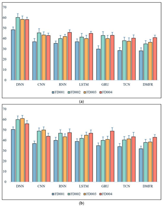
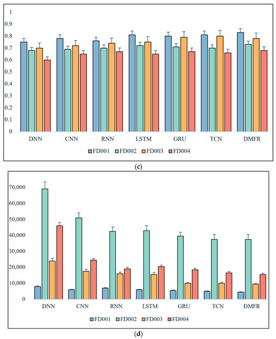
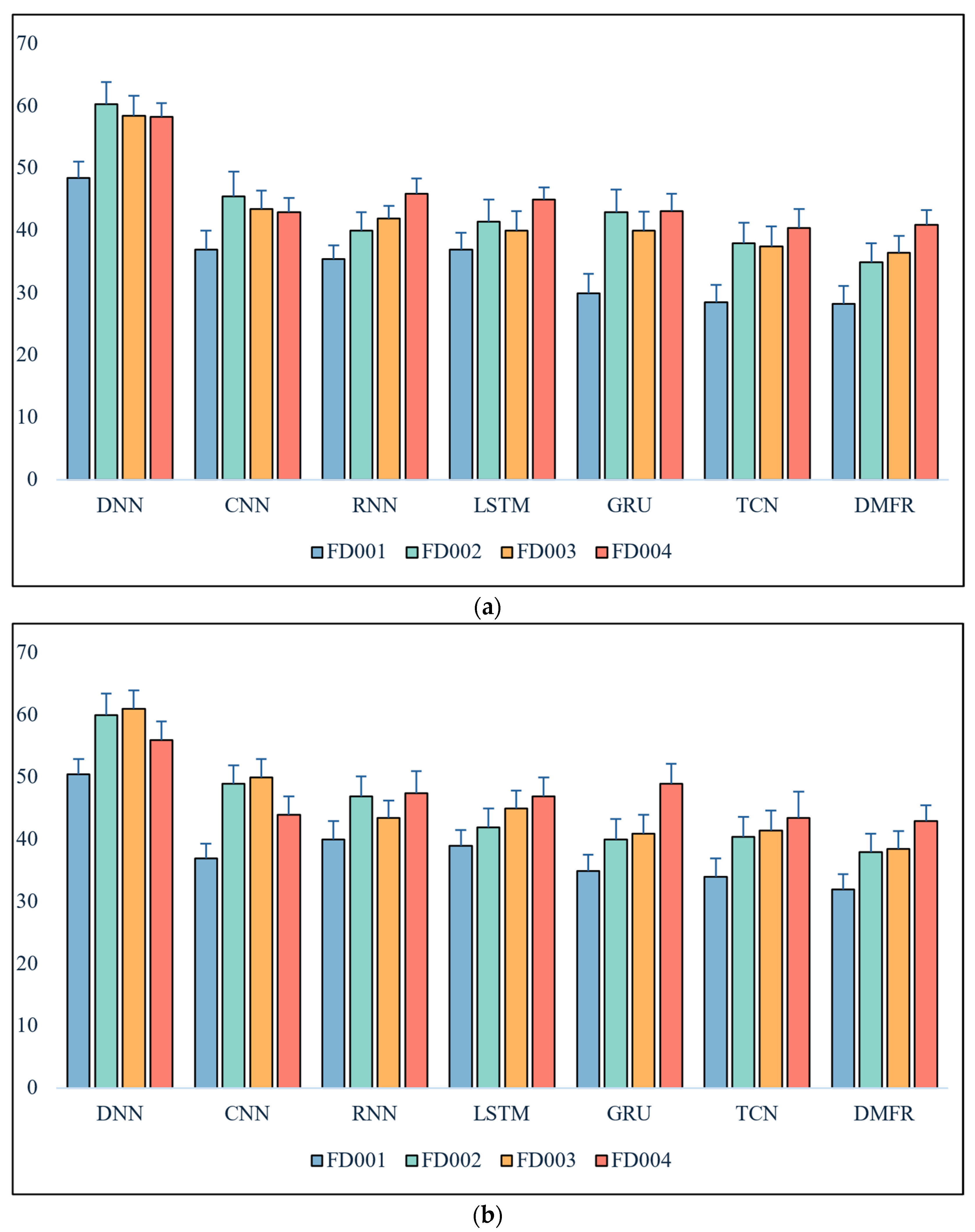
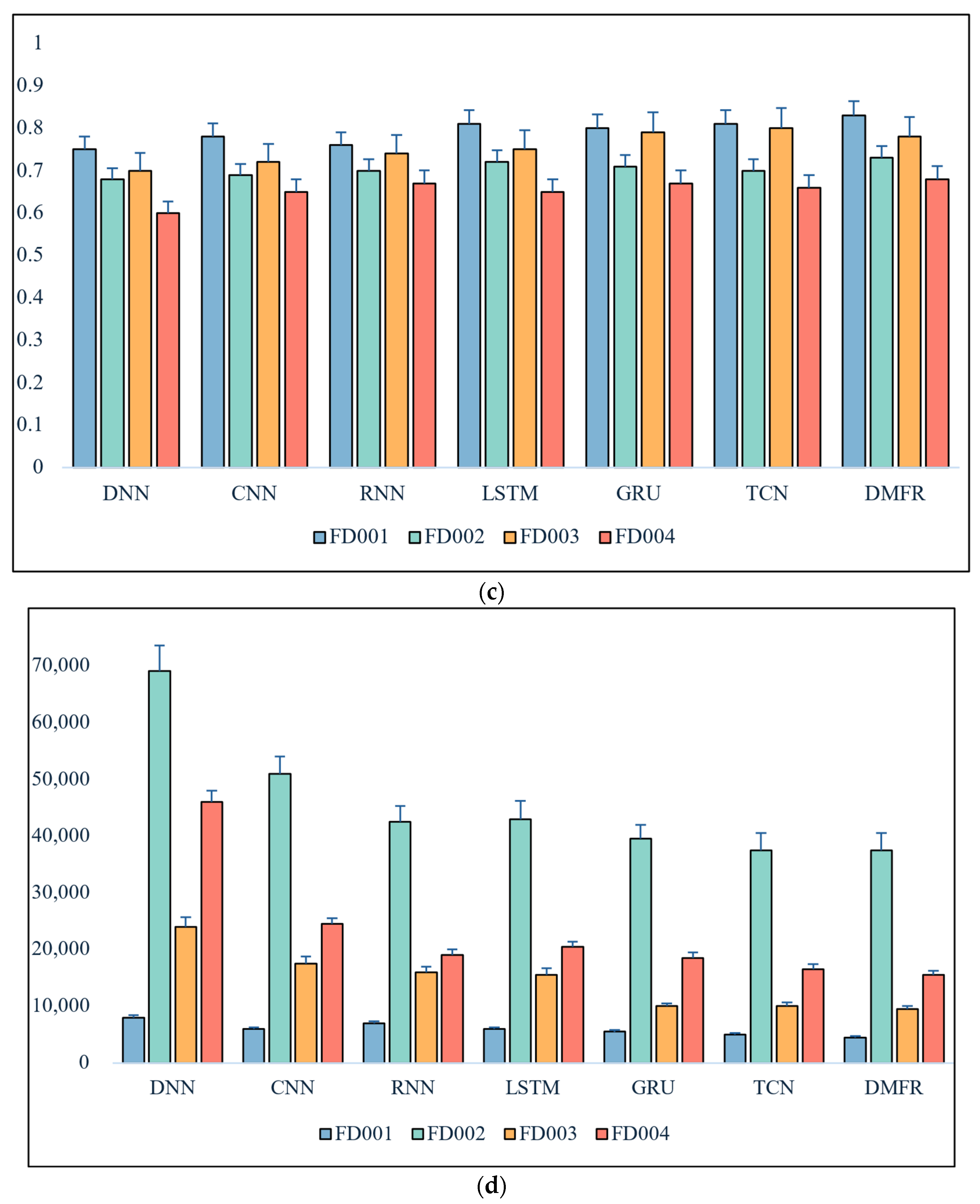
To validate the effectiveness of the transfer learning method in predicting the RUL of aircraft engines using the DMFR model, this study selected four sub-datasets—FD001, FD002, FD003, and FD004—from the C-MAPSS dataset as target domains and conducted comparative experiments with models such as CNN, DNN, GRU, LSTM, RNN, and TCN. In each experiment, 70% of the data were used as the training set, 15% as the validation set, and the remaining 15% as the test set. All models underwent hyperparameter tuning to ensure fairness in comparison. The experimental results are shown in Figure 5a–d. The bar charts report the mean performance across multiple runs, and the added error bars represent the standard deviation, indicating the stability of each model’s predictions.

Figure 5. (a) RMSE performance comparison under different target domains. (b) MAE performance comparison under different target domains. (c) R2 performance comparison under different target domains. (d) Score performance comparison under different target domains.

The experimental results demonstrate that the proposed DMFR model achieves the best prediction performance across all target domain settings. Specifically: (1) On the FD001 dataset, the DMFR model achieves an RMSE of 0.233, representing a 9.8% reduction compared with the second-best TCN model; (2) For the more complex FD003 dataset, the DMFR model maintains a significant advantage, with an average RMSE reduction of 10.5% compared with the baseline model; (3) Notably, as the complexity of the target domain data increases, the performance advantage of DMFR over other models expands, validating its strong cross-domain adaptability. The analysis suggests that DMFR effectively addresses the issue of insufficient feature extraction in complex operating conditions by deeply integrating temporal and spatial features and employing a dynamic weight adjustment mechanism.

4.5.3. Comparison of Different Modal Models

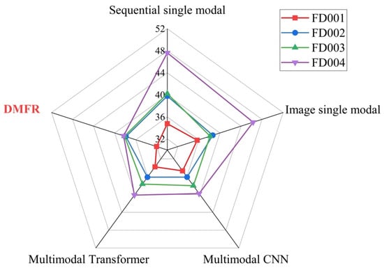
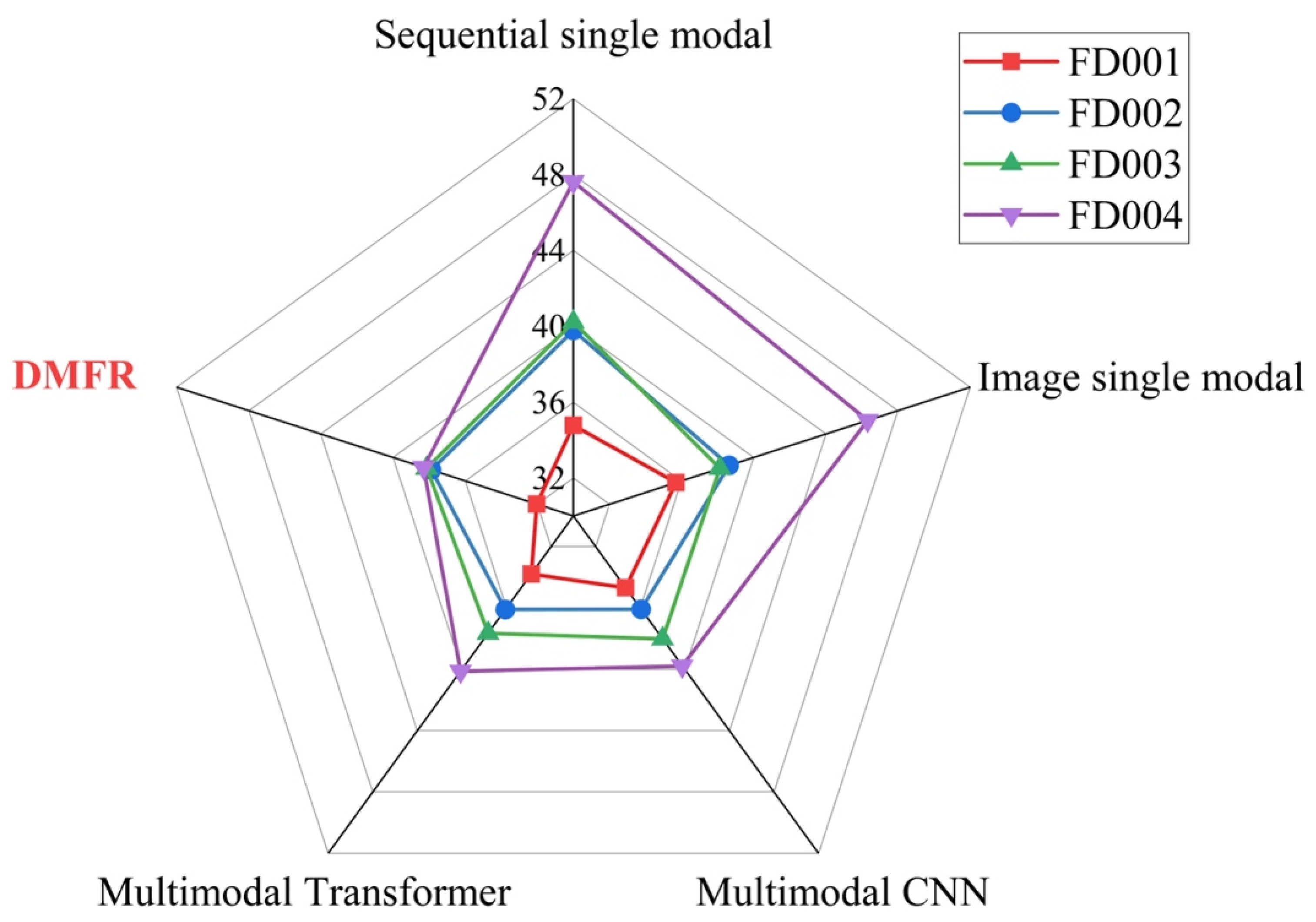
To validate the effectiveness of the multimodal fusion strategy, this study systematically compared the prediction performance of different modal transfer methods on the four sub-datasets (FD001–FD004) of the C-MAPSS dataset. Five comparison methods were set up: (1) Sequential single-modal transfer (using only Transformers to process sensor sequence data); (2) Image single-modal transfer (using only CNNs to process RP image data); (3) Multimodal CNN transfer (a dual-branch CNN architecture to process both modalities); (4) Multimodal Transformer transfer (a dual-branch Transformer architecture); (5) The DMFR method proposed in this study (a CNN–Transformer hybrid architecture). All experiments adopt the same training–validation–test split ratio (70%–15%–15%) and undergo rigorous hyperparameter tuning. As shown in Figure 6, the RMSE performance comparison of different methods across four target domains:

Figure 6. Comparison of RMSE performance of various methods under different target domains (DMFR is highlighted in red for clarity).

The experimental results fully demonstrate the superiority of the DMFR framework: (1) In all target domains, DMFR achieves the lowest RMSE values, with a reduction compared with the second-best method (multimodal Transformer) on FD001; (2) Among single-modal methods, the image modality outperforms the temporal modality overall, validating the effectiveness of RP plots in visualizing degenerate features; (3) Multimodal methods generally outperform single-modal methods, but pure CNN or pure Transformer multimodal architectures failed to fully leverage cross-modal synergy effects; (4) DMFR maintains a low RMSE under the complex conditions of FD003 through its innovative hybrid architecture design, significantly outperforming the RMSE of multimodal CNN. This indicates that the complementary feature extraction mechanisms of the CNN–Transformer can more comprehensively capture equipment degradation features, and its dynamic feature fusion strategy effectively enhances the robustness of cross-domain prediction.

5. Conclusions

The proposed DMFR framework provides an innovative solution for predicting the RUL of devices. By constructing a multimodal feature extraction module that integrates convolutional neural networks and Transformers, DMFR can fully capture the degradation patterns of different modal data and effectively overcome the representation limitations of single-modal data. With the help of a multimodal feature fusion layer and a two-stage transfer learning algorithm, DMFR achieves accurate transfer of source domain knowledge to the target domain, significantly enhancing the model’s generalization ability in small-sample and cross-condition scenarios. Comparative experiments on the NASA turbine engine dataset demonstrate that DMFR achieves significant performance improvements over traditional methods across multiple tasks, validating its effectiveness in achieving high-precision RUL prediction in complex industrial environments.

Looking ahead, we plan to further explore fusion strategies for more complex multimodal data types (such as vibration spectra, acoustic emission signals, and thermal imaging data) and develop more efficient transfer learning algorithms to adapt to the personalized needs of different industrial scenarios.

References

- Tsui, K.L.; Chen, N.; Zhou, Q.; Hai, Y.; Wang, W. Prognostics and health management: A review on data driven approaches. Math. Probl. Eng. 2015, 2015, 793161. [Google Scholar] [CrossRef] [Scilit]
- Hamadache, M.; Jung, J.H.; Park, J.; Youn, B.D. A comprehensive review of artificial intelligence-based approaches for rolling element bearing PHM: Shallow and deep learning. JMST Adv. 2019, 1, 125–151. [Google Scholar] [CrossRef] [Scilit]
- Liao, L.; Köttig, F. Review of hybrid prognostics approaches for remaining useful life prediction of engineered systems, and an application to battery life prediction. IEEE Trans. Reliab. 2014, 63, 191–207. [Google Scholar] [CrossRef] [Scilit]
- Lei, Y.; Li, N.; Guo, L.; Li, N.; Yan, T.; Lin, J. Machinery health prognostics: A systematic review from data acquisition to RUL prediction. Mech. Syst. Signal Process. 2018, 104, 799–834. [Google Scholar] [CrossRef] [Scilit]
- Mathew, V.; Toby, T.; Singh, V.; Rao, B.M.; Kumar, M.G. Prediction of Remaining Useful Lifetime (RUL) of turbofan engine using machine learning. In Proceedings of the 2017 IEEE International Conference on Circuits and Systems (ICCS), Thiruvananthapuram, India, 20–21 December 2017. [Google Scholar]
- Berghout, T.; Benbouzid, M. A systematic guide for predicting remaining useful life with machine learning. Electronics 2022, 11, 1125. [Google Scholar] [CrossRef] [Scilit]
- Esfahani, Z.; Salahshoor, K.; Farsi, B.; Eicker, U. A new hybrid model for RUL prediction through machine learning. J. Fail. Anal. Prev. 2021, 21, 1596–1604. [Google Scholar] [CrossRef] [Scilit]
- Wang, Y.; Zhao, Y.; Addepalli, S. Remaining useful life prediction using deep learning approaches: A review. Procedia Manuf. 2020, 49, 81–88. [Google Scholar] [CrossRef] [Scilit]
- Ma, M.; Mao, Z. Deep-convolution-based LSTM network for remaining useful life prediction. IEEE Trans. Ind. Inform. 2020, 17, 1658–1667. [Google Scholar] [CrossRef] [Scilit]
- Ren, L.; Cui, J.; Sun, Y.; Cheng, X. Multi-bearing remaining useful life collaborative prediction: A deep learning approach. J. Manuf. Syst. 2017, 43, 248–256. [Google Scholar] [CrossRef] [Scilit]
- Zhang, J.; Jiang, Y.; Wu, S.; Li, X.; Luo, H.; Yin, S. Prediction of remaining useful life based on bidirectional gated recurrent unit with temporal self-attention mechanism. Reliab. Eng. Syst. Saf. 2022, 221, 108297. [Google Scholar] [CrossRef] [Scilit]
- Fan, Y.; Nowaczyk, S.; Rögnvaldsson, T. Transfer learning for remaining useful life prediction based on consensus self-organizing models. Reliab. Eng. Syst. Saf. 2020, 203, 107098. [Google Scholar] [CrossRef] [Scilit]
- Wang, P.; Li, J.; Wang, S.; Zhang, F.; Shi, J.; Shen, C. A new meta-transfer learning method with freezing operation for few-shot bearing fault diagnosis. Meas. Sci. Technol. 2023, 34, 074005. [Google Scholar] [CrossRef] [Scilit]
- Zhang, Q.; Liu, Q.; Ye, Q. An attention-based temporal convolutional network method for predicting remaining useful life of aero-engine. Eng. Appl. Artif. Intell. 2024, 127, 107241. [Google Scholar] [CrossRef] [Scilit]
- Wang, Z.; Zhang, Z.; Zhang, H.; Liu, L.; Huang, R.; Cheng, X.; Zhao, H.; Zhao, Z. Omnibind: Large-scale omni multimodal representation via binding spaces. arXiv 2024, arXiv:2407.11895. [Google Scholar]
- Peng, C.; Sheng, Y.; Gui, W.; Tang, Z.; Li, C. A rolling bearing fault diagnosis method based on multimodal knowledge graph. IEEE Trans. Ind. Inform. 2024, 20, 13047–13057. [Google Scholar] [CrossRef] [Scilit]
- Li, H.; Huang, J.; Huang, J.; Chai, S.; Zhao, L.; Xia, Y. Deep multimodal learning and fusion based intelligent fault diagnosis approach. J. Beijing Inst. Technol. 2021, 30, 172–185. [Google Scholar]
- Wang, S.; Wang, B.; Zhang, Z.; Heidari, A.A.; Chen, H. Class-aware sample reweighting optimal transport for multi-source domain adaptation. Neurocomputing 2023, 523, 213–223. [Google Scholar] [CrossRef] [Scilit]
- Zhang, A.; Wang, H.; Li, S.; Cui, Y.; Liu, Z.; Yang, G.; Hu, J. Transfer learning with deep recurrent neural networks for remaining useful life estimation. Appl. Sci. 2018, 8, 2416. [Google Scholar] [CrossRef] [Scilit]
- Ding, Y.; Ding, P.; Zhao, X.; Cao, Y.; Jia, M. Transfer learning for remaining useful life prediction across operating conditions based on multisource domain adaptation. IEEE/ASME Trans. Mechatron. 2022, 27, 4143–4152. [Google Scholar] [CrossRef] [Scilit]
- Sun, C.; Ma, M.; Zhao, Z.; Tian, S.; Yan, R.; Chen, X. Deep transfer learning based on sparse autoencoder for remaining useful life prediction of tool in manufacturing. IEEE Trans. Ind. Inform. 2018, 15, 2416–2425. [Google Scholar] [CrossRef] [Scilit]
- Li, Z.-J.; Cheng, D.-J.; Zhang, H.-B.; Zhou, K.-L.; Wang, Y.-F. Multi-feature spaces cross adaption transfer learning-based bearings piece-wise remaining useful life prediction under unseen degradation data. Adv. Eng. Inform. 2024, 60, 102413. [Google Scholar] [CrossRef] [Scilit]
- Cao, Y.; Jia, M.; Ding, P.; Ding, Y. Transfer learning for remaining useful life prediction of multi-conditions bearings based on bidirectional-GRU network. Measurement 2021, 178, 109287. [Google Scholar] [CrossRef] [Scilit]
- Razzaghi, P.; Abbasi, K.; Shirazi, M.; Rashidi, S. Multimodal brain tumor detection using multimodal deep transfer learning. Appl. Soft Comput. 2022, 129, 109631. [Google Scholar] [CrossRef] [Scilit]
- Rahman, W.; Hasan, M.K.; Lee, S.; Zadeh, A.; Mao, C.; Morency, L.-P.; Hoque, E. Integrating multimodal information in large pretrained transformers. Proc. Conf. Assoc. Comput. Linguist. Meet. 2020, 2020, 2359–2369. [Google Scholar]
- Ji, T.; Vuppala, S.T.; Chowdhary, G.; Driggs-Campbell, K. Multi-modal anomaly detection for unstructured and uncertain environments. arXiv 2020, arXiv:2012.08637. [Google Scholar] [CrossRef] [Scilit]
- Marwan, N.; Romano, M.C.; Thiel, M.; Kurths, J. Recurrence plots for the analysis of complex systems. Phys. Rep. 2007, 438, 237–329. [Google Scholar] [CrossRef] [Scilit]
- da Costa, P.R.D.O.; Akçay, A.; Zhang, Y.; Kaymak, U. Remaining useful lifetime prediction via deep domain adaptation. Reliab. Eng. Syst. Saf. 2020, 195, 106682. [Google Scholar] [CrossRef] [Scilit]
- Ramasso, E.; Saxena, A. Review and analysis of algorithmic approaches developed for prognostics on CMAPSS dataset. In Proceedings of the Annual Conference of the Prognostics and Health Management Society 2014, Cheney, WA, USA, 22–25 June 2014. [Google Scholar]
- Vollert, S.; Theissler, A. Challenges of machine learning-based RUL prognosis: A review on NASA’s C-MAPSS data set. In Proceedings of the 2021 26th IEEE International Conference on Emerging Technologies and Factory Automation (ETFA), Västerås, Sweden, 7–10 September 2021. [Google Scholar]
Disclaimer/Publisher’s Note: The statements, opinions and data contained in all publications are solely those of the individual author(s) and contributor(s) and not of MDPI and/or the editor(s). MDPI and/or the editor(s) disclaim responsibility for any injury to people or property resulting from any ideas, methods, instructions or products referred to in the content. |
© 2025 by the authors. Licensee MDPI, Basel, Switzerland. This article is an open access article distributed under the terms and conditions of the Creative Commons Attribution (CC BY) license (https://creativecommons.org/licenses/by/4.0/).