Characterizing the Signless Laplacian H-Spectral Radius for Uniform Directed Hypergraphs

Abstract

The importance of the signless Laplacian H-spectral radius is highlighted by its known links to connectivity and the maximum cut and independence number. In this paper, we establish signless Laplacian H-spectral radius bounds by simultaneously incorporating both pairwise and higher-order outdegree information. In contrast to the important estimates based solely on the maximum outdegree, our approach yields substantially improved bounds by leveraging richer structural parameters. We further introduce outdegree regularity and semiregularity, under which the tightness of the proposed bounds is fully characterized. Based on similarity transformations, we construct improved bounds using average two-outdegree data. These bounds reveal distinct behaviors between the adjacency and signless Laplacian H-spectral radius of directed hypergraphs. Numerical examples are provided to illustrate the effectiveness of these bounds.

1. Introduction

Let $\mathbb{C}$ and $\mathbb{R}$ denote the sets of complex and real numbers, respectively, and let ${\mathbb{C}}^n$ and ${\mathbb{R}}^n$ denote the corresponding n-dimensional complex and real vector spaces, respectively. We write $\left[n\right]=\{1,2,\dots ,n\}$. An mth-order n-dimensional tensor $\mathcal{A}$ is an array of $n^m$ real entries $a_{i_1{i}_2\cdots i_m}\in \mathbb{R}$, where $i_j\in \left[n\right]$ for $j=1,\dots ,m$. If $a_{i_1\cdots i_m}=a_{i_{p(1)}\cdots i_{p(m)}}$ for every permutation p of $\left[m\right]$, then $\mathcal{A}$ is called a symmetric tensor. If all entries are nonnegative (positive), then $\mathcal{A}$ is called a nonnegative (positive) tensor.

A tensor is a higher-order extension of a matrix, which plays an important role in multilinear PageRank [1], higher-order Markov chains [2] and medical imaging [3,4]. Just as matrices serve as a fundamental tool for unveiling graph properties [5], tensors offer an indispensable framework for exploring the structural characteristics of hypergraphs [6,7]. To capture the properties of different undirected hypergraphs, signless Laplacian tensors and adjacency tensors have been established [6,8,9,10,11,12,13].

Unlike undirected hypergraphs, the edges (called arcs) in directed hypergraphs have directionality, capturing unidirectional relationships among nodes. As a generalization of directed graphs, directed hypergraphs find wide application in image processing [14,15] and social network analysis [16,17,18,19,20]. For example, hypergraph-based representations have been successfully used for feature extraction and segmentation in image processing. Formally, a k-uniform directed hypergraph $\overrightarrow{\mathbb{G}}=(\mathbb{V},\mathbb{E})$ consists of a vertex set $\mathbb{V}=\left[n\right]$ and an arc set $\mathbb{E}=\{e_1,\dots ,e_m\}$. Each arc $e\in \mathbb{E}$ has the form $e=(v_1,v_2,\dots ,v_k)$, where $v_1$ is the tail (out-vertex) and $v_2,\dots ,v_k$ are the heads (in-vertices). Accordingly, the associated adjacency or signless Laplacian tensor is assumed to be symmetric with respect to the last $k-1$ indices (or fully symmetric) to ensure a well-defined tensorial representation. The outdegree and indegree of a vertex i are defined as follows:

$$d_i^{+}=|{\mathbb{E}}_i^{+}|,d_i^{-}={\displaystyle \frac{1}{k-1}}\left|{\mathbb{E}}_i^{-}\right|,$$

where ${\mathbb{E}}_i^{+}=\{e\in \mathbb{E}:i\mathrm{is}\mathrm{the}\mathrm{tail}\mathrm{of}e\}$ and ${\mathbb{E}}_i^{-}=\{e\in \mathbb{E}:i\mathrm{is}\mathrm{one}\mathrm{of}\mathrm{the}\mathrm{heads}\mathrm{of}e\}$.

The pioneering work in [21] showed that k-uniform directed hypergraphs correspond bijectively to their adjacency tensors. Specifically, for a directed hypergraph $\overrightarrow{\mathbb{G}}=(\mathbb{V},\mathbb{E})$, the adjacency tensor $\mathcal{A}(\overrightarrow{\mathbb{G}})$ is a kth-order n-dimensional nonnegative tensor, whose $(i_1,\dots ,i_k)$-entry is defined by

$$\mathcal{A}{(\overrightarrow{\mathbb{G}})}_{i_1\dots i_k}=\left\{\begin{array}{cc}{\displaystyle \frac{1}{(k-1)!}},\hfill & \mathrm{if}(i_1,\dots ,i_k)=e\in \mathbb{E}\mathrm{and}{i}_1\mathrm{is}\mathrm{the}\mathrm{tail}\mathrm{of}e,\hfill \\ 0,\hfill & \mathrm{otherwise}.\hfill \end{array}\right.$$

The tensor is understood to be symmetric with respect to the last $k-1$ indices, and thus the ordering of the heads does not affect the representation.

However, the adjacency tensor reflects only the bare incidence pattern of arcs and ignores the outdegree of each vertex. In many contexts, the outdegree distribution is known to influence invariants such as expansion, the isoperimetric number and connectivity [22]. This shortcoming naturally motivates the introduction of the signless Laplacian tensor:

$$\mathcal{Q}(\overrightarrow{\mathbb{G}})={\mathcal{D}}^{+}+\mathcal{A}(\overrightarrow{\mathbb{G}}),$$

where ${\mathcal{D}}^{+}$ is the diagonal tensor of vertex outdegrees [23].

There is an extensive research on the H-spectral radius analysis of adjacency tensors for hypergraphs [8,9,23,24,25,26]. In contrast to the adjacency tensor, the signless Laplacian H-spectral radius encodes both the underlying connection structure and the weighted contribution of outdegrees [27], thus providing a more informative spectral measure. Its importance is reinforced by well-known relations to several hypergraph properties, including connectivity and the maximum cut and independence number [28,29]. These observations suggest that the signless Laplacian H-spectral radius is not merely of theoretical interest but also serves as an effective tool for investigating network integrity and extremal properties. From a theoretical perspective, the pursuit of tighter bounds is central to the characterization of extremal hypergraphs [20]. From a practical perspective, directed hypergraphs naturally model complex systems such as citation networks, social networks and biological networks, where spectral bounds are instrumental in assessing robustness and understanding propagation dynamics [19].

To rigorously study the H-spectral radius of tensors, we adopt the framework of H-eigenvalues introduced in [7,30]. A real pair $(\lambda ,x)$ is an H-eigenpair of an mth-order n-dimensional tensor $\mathcal{A}$ if

$$\mathcal{A}{x}^{m-1}=\lambda x^{[m-1]},$$

where ${(\mathcal{A}{x}^{m-1})}_i={\displaystyle \sum _{i_2,\dots ,i_m\in \left[n\right]}}{a}_{i{i}_2\dots i_m}{x}_{i_2}\cdots x_{i_m}$ and $x^{[m-1]}={[x_1^{m-1},\dots ,x_n^{m-1}]}^{\top }$.

The nonnegativity of $\mathcal{Q}(\overrightarrow{\mathbb{G}})$ guarantees that its H-spectral radius is the largest H eigenvalue from the Perron–Frobenius theorem [31]. Owing to the inherent asymmetry of the signless Laplacian tensor, standard optimization methods are inapplicable to the direct computation of its H-spectral radius [32]. Compounding this difficulty, determining the H-spectral radius for such structures is known to be NP-hard [7]. These obstacles have prompted a shift in research focus toward deriving upper and lower bounds on the H-spectral radius [21,23,25]. In this vein, Xie et al. [23] proposed an estimate for the signless Laplacian H-spectral radius associated with the directed hypergraph $\overrightarrow{\mathbb{G}}$ as follows:

$${\Delta }^{+}\le \rho (\mathcal{Q}(\overrightarrow{\mathbb{G}}))\le 2{\Delta }^{+},$$

where $\rho (\mathcal{Q}(\overrightarrow{\mathbb{G}}))$ is the signless Laplacian H-spectral radius and ${\Delta }^{+}=\underset{i\in \left[n\right]}{max}{d}_i^{+}$ is the maximum outdegree.

Bounding the signless Laplacian H-spectral radius solely by the maximum outdegree often yields crude estimates. To circumvent this limitation, we present a refined strategy that jointly employs multiple outdegree statistics. This strategy captures local structural correlations beyond the mere global maximum degree, thus leading to sharp bounds on the signless Laplacian H-spectral radius. In directed hypergraphs, multiple arcs with the same tail i may share the same head j, which is a distinctive property absent in ordinary graphs. Accordingly, we define $p_i(j)$ as the number of such arcs and utilize this multiplicity to refine the characterization of the signless Laplacian H-spectral radius, leading to improved bounds. Finally, similarity transformation can preserve tensor eigenvalues and enable a more precise characterization of the eigenvalues [31]. Hence, we employ similarity transformations to introduce the average two-outdegree as an extra structural parameter, which yields sharper bounds. Based on these observations, we establish new bounds of the signless Laplacian H-spectral radius with $O(mk+n)$ complexity and improve the existing results, where $m=\left|\mathbb{E}\right|$. Our main contributions are summarized as follows:

(1) We establish improved bounds for the signless Laplacian H-spectral radius in terms of the outdegree sums of two or more vertices and yield equality conditions that precisely characterize extremal directed hypergraphs.

(2) By exploiting parameters unique to directed hypergraphs, we construct new bounds that outperform the previous ones by capturing higher-order structural correlations beyond conventional degree-based approaches.

(3) By applying similarity transformations, we introduce the average two-outdegree as an additional parameter, leading to bounds of a different functional form.

(4) Numerical examples confirm the effectiveness and applicability of our theoretical results.

This paper proceeds as follows. In Section 2, we recall the notation and necessary preliminaries. We present the signless Laplacian H-spectral radius bounds based on double and multiple outdegrees in Section 3. Section 4 derives the new signless Laplacian H-spectral radius bounds via similarity transformations and average two-outdegree information. Section 5 concludes the paper.

2. Notation and Preliminaries

In this section, we review the fundamental definitions and properties concerning tensor eigenvalues and directed hypergraphs. Following [14,23], we define a directed hypergraph as one in which every arc has a single tail.

Definition 1.

For a k-uniform directed hypergraph $\overrightarrow{\mathbb{G}}=(\mathbb{V},\mathbb{E})$, we define the following concepts:

(1) Each arc has cardinality k.

(2) Two distinct vertices $v_i$ and $v_j$ are weakly connected if there exists a sequence of arcs $(e_1,\dots ,e_m)$ such that $v_i$ belongs to $e_1$, $v_j$ belongs to $e_m$ and $e_r\cap e_{r+1}\ne Ø$ for every $r\in [m-1]$. The directed hypergraph $\overrightarrow{\mathbb{G}}$ is called weakly connected if every pair of distinct vertices in $\mathbb{V}$ is weakly connected.

(3) For two distinct vertices $v_i$ and $v_j$, we write $v_i\to v_j$ if there exists a sequence of arcs $(e_1,\dots ,e_m)$ such that $v_i$ is the tail of $e_1$, $v_j$ is one of the heads of $e_m$ and for each $r\in [m-1]$, some head of $e_r$ is the tail of $e_{r+1}$. The directed hypergraph $\overrightarrow{\mathbb{G}}$ is called strongly connected if for every pair of distinct vertices $v_i,v_j\in \mathbb{V}$, we have both $v_i\to v_j$ and $v_j\to v_i$.

(4) For two distinct vertices $v_i$ and $v_j$, we say $i\sim j$ if there exists an arc with a tail $v_i$ and a head $v_j$. The out-neighborhood of $v_i$ is defined as $N^{+}(v_i)=\{v_j:i\sim j\}$, i.e., the set of all out-neighbors of $v_i$.

(5) For a subset $S\subseteq \mathbb{V}$, the directed subhypergraph of $\overrightarrow{\mathbb{G}}$ induced by S, denoted by ${\overrightarrow{\mathbb{G}}}_S$, is the directed hypergraph with a vertex set S and arc set $\{e\in \mathbb{E}:\mathit{all}\mathit{vertices}\mathit{of}e\mathit{lie}\mathit{in}S\}.$

Note that the outgoing arc set ${\mathbb{E}}_i^{+}$ denotes the set of all arcs with tail a $v_i$ (each of which may contain multiple heads). Hence, ${\mathbb{E}}_i^{+}$ is a collection of arcs, while $N^{+}(v_i)$ is a set of vertices. From the above definitions, it follows that every strongly connected directed hypergraph is also weakly connected. The example below shows that a weakly connected directed hypergraph need not be strongly connected.

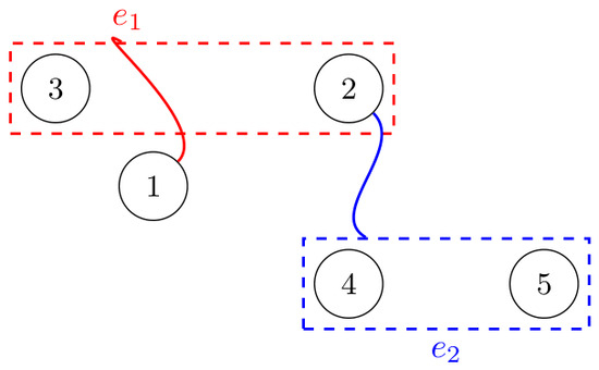
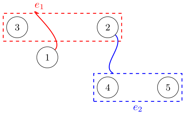
Let $\overrightarrow{\mathbb{G}}$ be a three-uniform directed hypergraph with a vertex set $\mathbb{V}=\{1,2,3,4,5\}$ and an arc set $\mathbb{E}=\{e_1,e_2\}$, where $e_1=(1,2,3),e_2=(2,4,5).$

Then, $\overrightarrow{\mathbb{G}}$ is weakly connected. For any pair of distinct vertices, one can find a sequence of arcs with nonempty intersections between consecutive arcs (e.g., $e_1$ and $e_2$ share vertex 2). However, $\overrightarrow{\mathbb{G}}$ is not strongly connected. To see this, we compute the out-neighborhoods:

$$N^{+}(1)=\{2,3\},N^{+}(2)=\{4,5\},N^{+}(3)=N^{+}(4)=N^{+}(5)=Ø.$$

Indeed, vertex 1 is the tail of $e_1$ only, and thus its out-neighbors are two and three; vertex 2 is the tail of $e_2$ only, so its out-neighbors are four and five; vertices $3,4,5$ are not tails of any arc; hence, their out-neighborhoods are empty. Because vertices $3,4,5$ have no outgoing arcs, they cannot initiate any directed path. In particular, there is no directed path from five (or four or three) to one, and thus the condition $v_i\to v_j$ fails for some ordered pairs. Therefore, $\overrightarrow{\mathbb{G}}$ is not strongly connected. Figure 1 provides a visualization.

Figure 1. Weakly connected 3-uniform directed hypergraph.

The following defines (generalized) regular directed hypergraphs [23,25].

Definition 2.

For a k-uniform directed hypergraph $\overrightarrow{\mathbb{G}}=(\mathbb{V},\mathbb{E})$, we introduce the following terminology:

(1) $\overrightarrow{\mathbb{G}}$ is called outdegree-regular (in-degree regular) if all $d_j^{+}$ ($d_j^{-}$) are equal to a common constant w.

(2) $\overrightarrow{\mathbb{G}}$ is called outdegree-semiregular if $\mathbb{V}=U\cup W$ with $U\cap W=Ø$, the outdegree of every vertex in U is $d_1^{+}$, that of every vertex in W is $d_2^{+}$ and the subhypergraphs induced by U and W are both empty (i.e., contain no arcs).

Outdegree regularity is clearly a special case of outdegree semiregularity. To facilitate the subsequent analysis, we recall that the signless Laplacian tensor $\mathcal{Q}(\overrightarrow{\mathbb{G}})$ is nonnegative and closely related to the hypergraph structure. We therefore summarize below several key properties of nonnegative tensors [10,33] that will be used later. Among these, two facts are particularly relevant. First, $\mathcal{A}(\mathbb{G})$ is weakly irreducible if and only if $\mathbb{G}$ is strongly connected. Second, the weak irreducibility of $\mathcal{A}(\mathbb{G})$ is equivalent to that of $\mathcal{Q}(\mathbb{G})$.

Lemma 1.

Let $\mathcal{A}$ be a nonnegative tensor. Then, $\rho (\mathcal{A})$ is an eigenvalue of $\mathcal{A}$ with a nonnegative eigenvector. Moreover, if $\mathcal{A}$ is weakly irreducible, then it admits a unique positive eigenvector x associated with $\rho (\mathcal{A})$ up to a positive scalar multiple.

In the following, we introduce similarity transformations and some important properties of tensors. Let $\mathcal{A}$ be an mth-order n-dimensional tensor and $D=diag(d_1,\dots ,d_n)$ be a positive diagonal matrix. We define ${\mathcal{A}}_D$ as the tensor obtained from $\mathcal{A}$ by multiplying each entry by $d_{i_1}^{1-m}{d}_{i_2}\cdots d_{i_m}$; that is, we have

$${({\mathcal{A}}_D)}_{i_1\cdots i_m}=a_{i_1\cdots i_m}{d}_{i_1}^{1-m}{d}_{i_2}\cdots d_{i_m}.$$

Lemma 2

(Theorem 2.8 of [31]). For two mth-order n-dimensional tensors $\mathcal{A}$ and $\mathcal{B}$, if there exists a nonsingular diagonal matrix D such that

$$\mathcal{B}=\mathcal{A}·D^{1-m}\underset{m-1}{\underbrace{D\cdots D}},$$

then $\mathcal{A}$ and $\mathcal{B}$ have identical eigenvalues.

3. Bounds for the Signless Laplacian $\mathit{H}$-Spectral Radius via Multiple (Two) Outdegrees

This section is devoted to deriving improved bounds for the signless Laplacian H-spectral radius by leveraging two or multiple outdegrees of a directed hypergraph. The proof framework for the subsequent theorems consists of three main steps: (1) selection of eigenvector components and characterization of their properties; (2) derivation of upper and lower bounds based on the chosen components and outdegree data and (3) investigation of the conditions under which equality is attained.

Theorem 1.

Let $\overrightarrow{\mathbb{G}}$ be a k-uniform directed hypergraph on n vertices. Then, we have the following:

(i) 

$$\begin{array}{c}\rho (\mathcal{Q}(\overrightarrow{\mathbb{G}}))\le \underset{e_i\in \mathbb{E}(\overrightarrow{\mathbb{G}})}{max}\underset{j\in e_i}{max}\{d_i^{+}+d_j^{+}\}.\hfill \end{array}$$

(1)

If $\overrightarrow{\mathbb{G}}$ is strongly connected, then

(ii) 

$$\rho (\mathcal{Q}(\overrightarrow{\mathbb{G}}))\ge \underset{e_i\in \mathbb{E}(\overrightarrow{\mathbb{G}})}{min}\underset{j\in e_i}{min}\{d_i^{+}+d_j^{+}\}.$$

(2)

Moreover, if $\overrightarrow{\mathbb{G}}$ is strongly connected, then equality holds in both Equations (1) and (2) if and only if $\overrightarrow{\mathbb{G}}$ is outdegree-semiregular.

Proof. 

(i) We establish the upper bound. Under Lemma 1, let $x={(x_1,\dots ,x_n)}^{\top }$ be a nonnegative eigenvector of $\mathcal{Q}(\overrightarrow{\mathbb{G}})$ corresponding to $\rho (\mathcal{Q}(\overrightarrow{\mathbb{G}})).$ Choose an index t such that $1=x_t=\underset{i\in \left[n\right]}{max}{x}_i$, and let s be an index satisfying $x_s=max\left\{x_j:j\in N^{+}(t)\right\}.$ From the tth equation of $\mathcal{Q}(\overrightarrow{\mathbb{G}})x^{k-1}=\rho (\mathcal{Q}(\overrightarrow{\mathbb{G}}))x^{[k-1]}$, we obtain

$$\begin{array}{c}\hfill \rho (\mathcal{Q}(\overrightarrow{\mathbb{G}}))x_t^{k-1}=d_t^{+}{x}_t^{k-1}+\sum _{(t,i_2,\dots ,i_k)\in e_t}{x}_{i_2}\dots x_{i_k}.\end{array}$$

(3)

It follows from $x_t=1$ and $x_s=max\left\{x_j:j\in N^{+}(t)\right\}$ that

$$\begin{array}{c}\hfill (\rho (\mathcal{Q}(\overrightarrow{\mathbb{G}}))-d_t^{+})\le d_t^{+}{x}_s^{k-1}.\end{array}$$

(4)

Similarly, from the sth equation, we have

$$\begin{array}{c}\hfill \rho (\mathcal{Q}(\overrightarrow{\mathbb{G}}))x_s^{k-1}=d_s^{+}{x}_s^{k-1}+\sum _{(s,i_2,\dots ,i_k)\in e_s}{x}_{i_2}\dots x_{i_k}\le d_s^{+}{x}_s^{k-1}+d_s^{+},\end{array}$$

which, after division by $x_s^{k-1}>0$ (the case $x_s=0$ is trivial; from the tth equation, we have $\rho (\mathcal{Q}(\overrightarrow{\mathbb{G}}))=d_t^{+}$), yields

$$\begin{array}{c}\hfill (\rho (\mathcal{Q}(\overrightarrow{\mathbb{G}}))-d_s^{+})x_s^{k-1}\le d_s^{+}.\end{array}$$

(5)

In Theorem 5.1 of [23], it was shown that

$${\Delta }^{+}\le \rho (\mathcal{Q}(\overrightarrow{\mathbb{G}}))\le 2{\Delta }^{+},$$

which implies $\rho (\mathcal{Q}(\overrightarrow{\mathbb{G}}))\ge max\{d_t^{+},d_s^{+}\}.$ Taking the product of Equations (4) and (5) yields

$$\begin{array}{c}\hfill (\rho (\mathcal{Q}(\overrightarrow{\mathbb{G}}))-d_t^{+})(\rho (\mathcal{Q}(\overrightarrow{\mathbb{G}}))-d_s^{+})\le d_t^{+}{d}_s^{+}.\end{array}$$

By solving the inequality above, we obtain

$$\begin{array}{c}\hfill \rho (\mathcal{Q}(\overrightarrow{\mathbb{G}}))\le d_t^{+}+d_s^{+},\end{array}$$

which implies

$$\begin{array}{c}\hfill \rho (\mathcal{Q}(\overrightarrow{\mathbb{G}}))\le \underset{e_i\in \mathbb{E}(\overrightarrow{\mathbb{G}})}{max}\underset{j\in e_i}{max}\{d_j^{+}+d_i^{+}\}.\end{array}$$

(ii) We establish the lower bound. According to Lemma 1, strong connectivity of $\overrightarrow{\mathbb{G}}$ implies that $\mathcal{Q}(\overrightarrow{\mathbb{G}})$ is weakly irreducible, which guarantees a positive eigenvector $x={(x_1,\dots ,x_n)}^{\top }$ associated with the signless Laplacian H-spectral radius $\rho (\mathcal{Q}(\overrightarrow{\mathbb{G}}))$. Choose t such that $1=x_t={min}_{i\in \left[n\right]}{x}_i$, and choose $s\in N^{+}(t)$ such that $x_s=min\{x_j:j\in N^{+}(t)\}$. Applying the same arguments as in the proofs of Equations (4) and (5) yields

$$\begin{array}{c}\hfill (\rho (\mathcal{Q}(\overrightarrow{\mathbb{G}}))-d_t^{+})\ge d_t^{+}{x}_s^{k-1},\end{array}$$

(6)

$$\begin{array}{c}\hfill (\rho (\mathcal{Q}(\overrightarrow{\mathbb{G}}))-d_s^{+})x_s^{k-1}\ge d_s^{+}.\end{array}$$

(7)

Taking the product of Equations (6) and (7) gives

$$\begin{array}{c}\hfill (\rho (\mathcal{Q}(\overrightarrow{\mathbb{G}}))-d_t^{+})(\rho (\mathcal{Q}(\overrightarrow{\mathbb{G}}))-d_s^{+})\ge d_t^{+}{d}_s^{+}.\end{array}$$

By solving the inequality above, one has

$$\begin{array}{c}\hfill \rho (\mathcal{Q}(\overrightarrow{\mathbb{G}}))\ge d_t^{+}+d_s^{+}.\end{array}$$

and therefore

$$\begin{array}{c}\hfill \rho (\mathcal{Q}(\overrightarrow{\mathbb{G}}))\ge \underset{e_i\in \mathbb{E}(\overrightarrow{\mathbb{G}})}{min}\underset{j\in e_i}{min}\{d_j^{+}+d_i^{+}\}.\end{array}$$

(iii) It remains to characterize equality. Suppose equality holds in Equation (1). From the derivation of Equation (4), equality forces $x_j=x_s$ for every $j\in N^{+}(t)$; similarly, equality in Equation (5) forces $x_j=x_t=1$ for every $j\in N^{+}(s)$. We distinguish two cases.

Case I: $x_s=1.$ Let $\tilde{V}=\{v_k:x_k=1\}$. If $\tilde{V}\ne \mathbb{V}$, then strong connectivity implies the existence of vertices $r,p\in \tilde{V}$ and $q\notin \tilde{V}$ with $(r\sim p)\in \mathbb{E}$ and $(p\sim q)\in \mathbb{E}$. Therefore, for the tail vertices $r,p\in \tilde{V}$, we obtain

$$(\rho (\mathcal{Q}(\overrightarrow{\mathbb{G}}))-d_r^{+})=\sum _{(r,i_2,\dots ,i_k)\in e_r}{x}_{i_2}\dots x_{i_k}\le d_r^{+},$$

$$(\rho (\mathcal{Q}(\overrightarrow{\mathbb{G}}))-d_p^{+})=\sum _{(p,i_2,\dots ,i_k)\in e_p}{x}_{i_2}\dots x_{i_k}<d_p^{+}.$$

Substituting these relations into the eigenvalue equations gives a strict inequality $\rho (\mathcal{Q}(\overrightarrow{\mathbb{G}}))<d_r^{+}+d_p^{+}$, contradicting the equality in Equation (1). Thus, $\tilde{V}=\mathbb{V}$, and so all outdegrees are equal, and $\overrightarrow{\mathbb{G}}$ is outdegree-semiregular.

Case II: $x_s<1.$ Then, $x_k=1$ for every $v_k\in N^{+}(v_s)$, and $x_j=x_s$ for every $v_j\in N^{+}(v_t)$. Define

$$U=\{v_k:x_k=1\}\mathrm{and}W=\{v_j:x_j=x_s\}.$$

Clearly, $N^{+}(v_s)\subseteq U$ and $N^{+}(v_t)\subseteq W$. For any $v_r\in N^{+}(N^{+}(v_t))$, choose $v_p\in N^{+}(v_t)$ with $(t\sim p),(p\sim r)\in \mathbb{E}(\overrightarrow{\mathbb{G}})$. Then, using $x_p=x_s$ in the H-eigenvalue equations, we obtain

$$(\rho (\mathcal{Q}(\overrightarrow{\mathbb{G}}))-d_p^{+})x_p^{k-1}=\sum _{(p,i_2,\dots ,i_k)\in e_p}{x}_{i_2}\dots x_{i_k}\le d_p^{+}$$

and

$$(\rho (\mathcal{Q}(\overrightarrow{\mathbb{G}}))-d_t^{+})=\sum _{(t,i_2,\dots ,i_k)\in e_t}{x}_{i_2}\dots x_{i_k}\le d_t^{+}{x}_s^{k-1}=d_t^{+}{x}_p^{k-1}.$$

Equivalently, we have

$$(\rho (\mathcal{Q}(\overrightarrow{\mathbb{G}}))-d_p^{+})x_p^{k-1}\le d_p^{+}{x}_t^{k-1} \mathrm{and} (\rho (\mathcal{Q}(\overrightarrow{\mathbb{G}}))-d_t^{+})x_t^{k-1}\le d_t^{+}{x}_p^{k-1},$$

which imply $\rho (\mathcal{Q}(\overrightarrow{\mathbb{G}}))\le d_t^{+}+d_p^{+}$. Suppose that $\rho (\mathcal{Q}(\overrightarrow{\mathbb{G}}))=\underset{e_i\in \mathbb{E}(\overrightarrow{\mathbb{G}})}{max}\underset{j\in e_i}{max}\{d_i^{+}+d_j^{+}\}.$ For any $(t\sim p)$, it holds that

$$\rho (\mathcal{Q}(\overrightarrow{\mathbb{G}}))\ge d_t^{+}+d_p^{+}.$$

Consequently, $\rho (\mathcal{Q}(\overrightarrow{\mathbb{G}}))=d_t^{+}+d_p^{+}.$ Therefore, the following equations hold simultaneously:

$$\begin{array}{c}\hfill (\rho (\mathcal{Q}(\overrightarrow{\mathbb{G}}))-d_p^{+})x_p^{k-1}=\sum _{(p,i_2,\dots ,i_k)\in e_p}{x}_{i_2}\dots x_{i_k}=d_p^{+}\end{array}$$

(∗)

$$\begin{array}{c}\hfill (\rho (\mathcal{Q}(\overrightarrow{\mathbb{G}}))-d_t^{+})=\sum _{(t,i_2,\dots ,i_k)\in e_t}{x}_{i_2}\dots x_{i_k}=d_t^{+}{x}_s^{k-1}=d_t^{+}{x}_p^{k-1}.\end{array}$$

(∗∗)

Since $x_r\in N^{+}(v_p),$ from $(\ast )$, we obtain

$$(\rho (\mathcal{Q}(\overrightarrow{\mathbb{G}}))-d_p^{+})x_p^{k-1}=\sum _{(p,i_2,r\dots ,i_k)\in e_p}{x}_{i_2}{x}_r\dots x_{i_k}=d_p^{+}$$

We employ a proof by contradiction to establish that $x_r=1.$ Otherwise, $x_r<1,$ and one has

$$(\rho (\mathcal{Q}(\overrightarrow{\mathbb{G}}))-d_p^{+})x_p^{k-1}=\sum _{(p,i_2,r\dots ,i_k)\in e_p}{x}_{i_2}{x}_r\dots x_{i_k}<d_p^{+}.$$

This, together with $(\ast \ast )$, yields

$$\rho (\mathcal{Q}(\overrightarrow{\mathbb{G}}))<d_t^{+}+d_p^{+},$$

which contradicts $\rho (\mathcal{Q}(\overrightarrow{\mathbb{G}}))=d_t^{+}+d_p^{+}.$ Thus, $x_r=1$ and $N^{+}(N^{+}(v_t))\subseteq U.$ Arguing analogously for the case $x_r=1$ yields $N^{+}(N^{+}(v_s))\subseteq W$. By iterating this procedure and using the strong connectivity of $\overrightarrow{\mathbb{G}}$, we conclude that $\mathbb{V}=U\cup W$, with the subhypergraphs induced by U and W being arc-free. Moreover, the outdegree is constant on each of the two parts, which implies that $\overrightarrow{\mathbb{G}}$ is outdegree-semiregular.

Conversely, under the assumption of strong connectivity, the two-sided inequality in Equations (1) and (2) is satisfied:

$$\underset{e_i\in \mathbb{E}(\overrightarrow{\mathbb{G}})}{min}\underset{j\in e_i}{min}\{d_i^{+}+d_j^{+}\}\le \rho (\mathcal{Q}(\overrightarrow{\mathbb{G}}))\le \underset{e_i\in \mathbb{E}(\overrightarrow{\mathbb{G}})}{max}\underset{j\in e_i}{max}\{d_i^{+}+d_j^{+}\}.$$

Now, assume further that $\overrightarrow{\mathbb{G}}$ is outdegree-semiregular with bipartition $\mathbb{V}=U\cup W$. In this case, every arc must have its tail in one part and all its heads in the other so that $d_i^{+}+d_j^{+}$ is constant over all admissible pairs $(i,j)$ with $j\in e_i$. Consequently, both bounds coincide with $\rho (\mathcal{Q}(\overrightarrow{\mathbb{G}}))$, and equality holds. □

Remark 1.

For a k-uniform directed hypergraph, with ${\Delta }^{+}=\underset{i\in \left[n\right]}{max}{d}_i^{+}$ denoting the maximum outdegree, it holds that

$$\rho (\mathcal{Q}(\overrightarrow{\mathbb{G}}))\le \underset{e_i\in \mathbb{E}(\overrightarrow{\mathbb{G}})}{max}\underset{j\in e_i}{max}\{d_i^{+}+d_j^{+}\}\le 2{\Delta }^{+}.$$

This directly implies that the bounds in Theorem 1 are sharper than those of Theorem 5.1 in [23].

Example 1.

Let ${\overrightarrow{\mathbb{G}}}_1$ be a three-uniform directed hypergraph on five vertices with the following outgoing arcs:

$$\begin{array}{cccccccc}\mathit{Tail}& 1& 1& 2& 2& 3& 4& 5\\ \mathit{Heads}& \{4,3\}& \{5,4\}& \{3,5\}& \{4,5\}& \{1,2\}& \{1,2\}& \{1,2\}\end{array}$$

We verify that ${\overrightarrow{\mathbb{G}}}_1$ is strongly connected and

$$d_1^{+}=d_2^{+}=2,d_3^{+}=d_4^{+}=d_5^{+}=1,$$

which implies $U=\{1,2\}$, $W=\{3,4,5\}$ and $U\cap W=Ø.$ Furthermore, the subhypergraphs induced by U and W are empty, which shows that ${\overrightarrow{\mathbb{G}}}_1$ is outdegree-semiregular. Since the outdegrees $d_i^{+}$ are not all equal to a common constant, ${\overrightarrow{\mathbb{G}}}_1$ is not outdegree-regular. Using Theorem 1, we obtain

$$\rho (\mathcal{Q}({\overrightarrow{\mathbb{G}}}_1))=3.0000.$$

Compared with the precise bounds of Theorem 1, the estimation for $\rho (\mathcal{Q}({\overrightarrow{\mathbb{G}}}_1))$ provided by Theorem 5.1 of [23] is as follows:

$$2.0000\le \rho (\mathcal{Q}({\overrightarrow{\mathbb{G}}}_1))\le 4.0000.$$

This example illustrates the sharpness of our bounds when the structural assumptions (outdegree semiregularity) are met.

Unlike directed graphs, where each pair $(i,j)$ appears in at most one arc, a directed hypergraph can have multiple arcs with the same tail i containing the same head j. To account for this multiplicity, we define $p_i(j)$ as the number of arcs with a tail i that contain j as a head. Selecting the second largest component of the eigenvector is also time-consuming, and thus we choose an arbitrary component $x_s$ of the eigenvector x to estimate the signless Laplacian H-spectral radius. To state the theorem more clearly, we introduce the following definition.

For every arc $e_i\in E(\overrightarrow{\mathbb{G}})$ and every vertex $j\in e_i$, define

$$M_{ij}=max\{d_j^{+},2d_i^{+}-p_i(j)\}.$$

Let ${\alpha }_{ij}$ be the largest real root in $[M_{ij},\infty )$ of the equation

$$(\lambda -d_j^{+}){\left(\lambda -(2d_i^{+}-p_i(j))\right)}^{k-1}=p_i{(j)}^{k-1}{d}_j^{+}.$$

Equivalently, ${\alpha }_{ij}$ can be written as

$${\alpha }_{ij}=max\left\{\lambda \in \mathbb{R}:(\lambda -d_j^{+}){\left(\lambda -(2d_i^{+}-p_i(j))\right)}^{k-1}\le p_i{(j)}^{k-1}{d}_j^{+}\right\}.$$

Theorem 2.

Let $\overrightarrow{\mathbb{G}}$ be a k-uniform directed hypergraph on n vertices. Then, we have

(i) 

$$\begin{array}{c}\rho (\mathcal{Q}(\overrightarrow{\mathbb{G}}))\le \underset{e_i\in \mathbb{E}(\overrightarrow{\mathbb{G}})}{max}\underset{j\in e_i}{min}{\alpha }_{ij}.\hfill \end{array}$$

(8)

If $\overrightarrow{\mathbb{G}}$ is strongly connected, then

(ii) 

$$\begin{array}{c}\rho (\mathcal{Q}(\overrightarrow{\mathbb{G}}))\ge \underset{e_i\in \mathbb{E}(\overrightarrow{\mathbb{G}})}{min}\underset{j\in e_i}{max}{\alpha }_{ij}.\hfill \end{array}$$

(9)

Moreover, if $\overrightarrow{\mathbb{G}}$ is outdegree-regular with a common outdegree w, then $\rho (\mathcal{Q}(\overrightarrow{\mathbb{G}}))=2w$.

Proof. 

(i) We establish the upper bound. According to Lemma 1, let $x={(x_1,\dots ,x_n)}^{\top }$ be a nonnegative eigenvector of $\mathcal{Q}(\overrightarrow{\mathbb{G}})$ corresponding to $\rho (\mathcal{Q}(\overrightarrow{\mathbb{G}})).$ Define an index t such that $x_t=\underset{i\in \left[n\right]}{max}{x}_i$ and an arbitrary vertex $s\in N^{+}(t)$. From the tth equation of $\mathcal{Q}(\overrightarrow{\mathbb{G}})x^{k-1}=\rho (\mathcal{Q}(\overrightarrow{\mathbb{G}}))x^{[k-1]}$, one has

$$\begin{array}{cc}\hfill \rho (\mathcal{Q}(\overrightarrow{\mathbb{G}}))x_t^{k-1}& =d_t^{+}{x}_t^{k-1}+\sum _{\{t,i_2,\dots ,i_k\}\in e_t}{x}_{i_2}\cdots x_{i_k}\hfill \\ \hfill & =d_t^{+}{x}_t^{k-1}+\sum _{\begin{array}{c}\{t,i_2,\dots ,i_k\}\in e_t\\ s\in \{i_2,\dots ,i_k\}\end{array}}{x}_{i_2}\cdots x_s\cdots x_{i_k}+\sum _{\begin{array}{c}\{t,i_2,\dots ,i_k\}\in e_t\\ s\notin \{i_2,\dots ,i_k\}\end{array}}{x}_{i_2}\cdots x_{i_k}\hfill \\ \hfill & \le d_t^{+}{x}_t^{k-1}+p_t(s)x_s{x}_t^{k-2}+(d_t^{+}-p_t(s))x_t^{k-1},\hfill \end{array}$$

which shows that

$$\begin{array}{c}\hfill (\rho (\mathcal{Q}(\overrightarrow{\mathbb{G}}))-(2d_t^{+}-p_t(s)))x_t\le p_t(s)x_s.\end{array}$$

(10)

We proceed by considering two cases:

Case I: $x_s=0$. Then, Equation (10) reduces to

$$\rho (\mathcal{Q}(\overrightarrow{\mathbb{G}}))\le 2d_t^{+}-p_t(s).$$

By the definition of ${\alpha }_{ts}$, we have ${\alpha }_{ts}\ge M_{ts}\ge 2d_t^{+}-p_t(s)$, and hence

$$\rho (\mathcal{Q}(\overrightarrow{\mathbb{G}}))\le {\alpha }_{ts}.$$

Case II: $x_s>0$. From Equation (10), if $\rho (\mathcal{Q}(\overrightarrow{\mathbb{G}}))-(2d_t^{+}-p_t(s))\le 0$, then

$$\rho (\mathcal{Q}(\overrightarrow{\mathbb{G}}))\le 2d_t^{+}-p_t(s)\le M_{ts}\le {\alpha }_{ts},$$

and the desired inequality for this s follows. Otherwise, the factor is positive, and raising both sides of Equation (10) to the $(k-1)$th power yields

$$\begin{array}{c}\hfill {(\rho (\mathcal{Q}(\overrightarrow{\mathbb{G}}))-(2d_t^{+}-p_t(s)))}^{k-1}{x}_t^{k-1}\le p_t{(s)}^{k-1}{x}_s^{k-1}.\end{array}$$

(11)

Under the sth equation of $\mathcal{Q}(\overrightarrow{\mathbb{G}})x^{[k-1]}=\rho (\mathcal{Q}(\overrightarrow{\mathbb{G}}))x^{[k-1]}$, it holds that

$$\begin{array}{cc}\hfill \rho (\mathcal{Q}(\overrightarrow{\mathbb{G}}))x_s^{k-1}& =d_s^{+}{x}_s^{k-1}+\sum _{\{s,i_2,\dots ,i_k\}\in e_s}{x}_{i_2}\cdots x_{i_k}\le d_s^{+}{x}_t^{k-1},\hfill \end{array}$$

That is, we have

$$\begin{array}{cc}\hfill (\rho (\mathcal{Q}(\overrightarrow{\mathbb{G}}))-d_s^{+})x_s^{k-1}& \le d_s^{+}{x}_t^{k-1}.\hfill \end{array}$$

(12)

Multiplying Equations (11) and (12) gives

$$\begin{array}{c}\hfill (\rho (\mathcal{Q}(\overrightarrow{\mathbb{G}}))-d_s^{+}){\left(\rho (\mathcal{Q}(\overrightarrow{\mathbb{G}}))-(2d_t^{+}-p_t(s))\right)}^{k-1}\le p_t{(s)}^{k-1}{d}_s^{+}.\end{array}$$

(13)

Define

$$f(\lambda )=(\lambda -d_s^{+}){\left(\lambda -(2d_t^{+}-p_t(s))\right)}^{k-1}.$$

Then, f is continuous and strictly increasing on $[M_{ts},\infty )$. If $\rho (\mathcal{Q}(\overrightarrow{\mathbb{G}}))\le M_{ts}$, then again, $\rho (\mathcal{Q}(\overrightarrow{\mathbb{G}}))\le {\alpha }_{ts}$ because ${\alpha }_{ts}\ge M_{ts}$. If $\rho (\mathcal{Q}(\overrightarrow{\mathbb{G}}))>M_{ts}$. Then, from Equation (13), we have

$$f\left(\rho (\mathcal{Q}(\overrightarrow{\mathbb{G}}))\right)\le p_t{(s)}^{k-1}{d}_s^{+}.$$

Since ${\alpha }_{ts}$ is the largest real number satisfying

$$f(\lambda )\le p_t{(s)}^{k-1}{d}_s^{+},$$

and f is increasing on $[M_{ts},\infty )$, it follows that

$$\rho (\mathcal{Q}(\overrightarrow{\mathbb{G}}))\le {\alpha }_{ts}.$$

Thus, in all cases, we obtain $\rho (\mathcal{Q}(\overrightarrow{\mathbb{G}}))\le {\alpha }_{ts}$ for the chosen s. Since s was arbitrary in $N^{+}(t)$, we get

$$\rho (\mathcal{Q}(\overrightarrow{\mathbb{G}}))\le \underset{j\in e_t}{min}{\alpha }_{tj}.$$

Taking the maximum over all arcs $e_i\in \mathbb{E}(\overrightarrow{\mathbb{G}})$ yields

$$\rho (\mathcal{Q}(\overrightarrow{\mathbb{G}}))\le \underset{e_i\in \mathbb{E}(\overrightarrow{\mathbb{G}})}{max}\underset{j\in e_i}{min}{\alpha }_{ij}.$$

(ii) We establish the lower bound. Under Lemma 1, strong connectivity of $\overrightarrow{\mathbb{G}}$ implies that $\mathcal{Q}(\overrightarrow{\mathbb{G}})$ is weakly irreducible, which guarantees a positive eigenvector $x={(x_1,\dots ,x_n)}^{\top }$ associated with the signless Laplacian H-spectral radius $\rho (\mathcal{Q}(\overrightarrow{\mathbb{G}}))$. Define an index t such that $x_t=\underset{i\in \left[n\right]}{min}{x}_i$ and an arbitrary vertex $s\in N^{+}(t)$. From the same reasoning that led to Equations (10) and (12), we obtain

$$\begin{array}{c}\hfill (\rho (\mathcal{Q}(\overrightarrow{\mathbb{G}}))-d_s^{+})x_s^{k-1}\ge d_s^{+}{x}_t^{k-1},\end{array}$$

(14)

and

$$(\rho (\mathcal{Q}(\overrightarrow{\mathbb{G}}))-(2d_t^{+}-p_t(s)))x_t\ge p_t(s)x_s.$$

Since $x_t>0$ and $p_t(s)x_s\ge 0$, the factors $\rho (\mathcal{Q}(\overrightarrow{\mathbb{G}}))-(2d_t^{+}-p_t(s))$ and $\rho (\mathcal{Q}(\overrightarrow{\mathbb{G}}))-d_s^{+}$ are nonnegative. Therefore, $\rho (\mathcal{Q}(\overrightarrow{\mathbb{G}}))\ge M_{ts}.$ Taking the $(k-1)$th power preserves the inequality direction and yields

$$\begin{array}{c}\hfill {(\rho (\mathcal{Q}(\overrightarrow{\mathbb{G}}))-(2d_t^{+}-p_t(s)))}^{k-1}{x}_t^{k-1}\ge p_t{(s)}^{k-1}{x}_s^{k-1}.\end{array}$$

(15)

The positivity of $x_s^{k-1}$ and $x_t^{k-1}$, together with $p_t(s)\ge 0$, allows us to multiply Equations (14) and (15), yielding

$$\begin{array}{c}\hfill (\rho (\mathcal{Q}(\overrightarrow{\mathbb{G}}))-d_s^{+}){\left(\rho (\mathcal{Q}(\overrightarrow{\mathbb{G}}))-(2d_t^{+}-p_t(s))\right)}^{k-1}\ge p_t{(s)}^{k-1}{d}_s^{+}.\end{array}$$

(16)

We verify that f is increasing on the interval $[M_{ts},\infty )$, and Equation (16) is exactly

$$f\left(\rho (\mathcal{Q}(\overrightarrow{\mathbb{G}}))\right)\ge p_t{(s)}^{k-1}{d}_s^{+}.$$

By the definition of ${\alpha }_{ts}$ as the largest real number satisfying

$$f(\lambda )\le p_t{(s)}^{k-1}{d}_s^{+},$$

the monotonicity of f on $[M_{ts},\infty )$ implies

$$\rho (\mathcal{Q}(\overrightarrow{\mathbb{G}}))\ge {\alpha }_{ts}.$$

Since s was chosen arbitrarily from $N^{+}(t)$, the above inequality holds for every $j\in e_t$. Therefore, we have

$$\rho (\mathcal{Q}(\overrightarrow{\mathbb{G}}))\ge \underset{j\in e_t}{max}{\alpha }_{tj}.$$

Taking the minimum over all arcs yields

$$\rho (\mathcal{Q}(\overrightarrow{\mathbb{G}}))\ge \underset{e_i\in \mathbb{E}(\overrightarrow{\mathbb{G}})}{min}\underset{j\in e_i}{max}{\alpha }_{ij}.$$

(iii) It remains to verify that $\rho (\mathcal{Q}(\overrightarrow{\mathbb{G}}))=2w$. If $\overrightarrow{\mathbb{G}}$ is outdegree-regular with $d_i^{+}=w$, then we confirm that the equation

$$f(\lambda )=(\lambda -w){(\lambda -(2w-p_i(j)))}^{k-1}=p_i{(j)}^{k-1}w$$

has a positive real root, namely $\lambda =2w$, for any integer $p_i(j)\in [1,w]$. A direct substitution gives

$$f(2w)=w·p_i{(j)}^{k-1}=p_i{(j)}^{k-1}w,$$

which shows that $\lambda =2w$ is indeed a root of the equation. Thus, $\rho (\mathcal{Q}(\overrightarrow{\mathbb{G}}))\ge 2w.$ Under the assumption that $\overrightarrow{\mathbb{G}}$ is outdegree-regular with a common outdegree w, we have ${\Delta }^{+}=w$, and hence $\rho (\mathcal{Q}(\overrightarrow{\mathbb{G}}))\le 2w$. Thus, the upper bound is exactly $2w$. □

Remark 2.

(i) In contrast to directed graphs, where $p_i(j)\le 1$, a directed hypergraph has $p_i(j)\le d_i^{+}$, which can be advantageous for bounding the spectral radius.

(ii) A distinctive feature of our approach is that the proof of Theorem 2 does not require $x_s$ to be the second largest component of the eigenvector; the inequality holds for any chosen component $s\in N^{+}(t)$. This is achieved by splitting the arcs with tail i into two classes according to whether they contain s or not, which yields the inequality

$$(\rho (\mathcal{Q}(\overrightarrow{\mathbb{G}}))-(2d_i^{+}-p_i(s)))x_i\le p_i(s)x_s,$$

This is valid for an arbitrary choice of s. Consequently, no optimality or ordering condition on $x_s$ is needed. This flexibility is a direct mathematical consequence of the classification argument rather than an additional assumption. In contrast to existing approaches that require identifying the second largest eigencomponent (e.g., the proof of Theorem 5.1 in [23]), our method avoids this step entirely, thereby reducing the computational cost while maintaining the validity of the bounds.

(iii) For a k-uniform directed hypergraph, from Equation (8), there exists $i\in \left[n\right]$ such that

$$(\rho (\mathcal{Q}(\overrightarrow{\mathbb{G}}))-d_j^{+}){(\rho (\mathcal{Q}(\overrightarrow{\mathbb{G}}))-(2d_i^{+}-p_i(j)))}^{k-1}\le p_i{(j)}^{k-1}{d}_j^{+}\mathit{for}\mathit{all}j\in e_i.$$

If $p_i(j)=0$, then the inequality yields either

$$\rho (\mathcal{Q}(\overrightarrow{\mathbb{G}}))=d_j^{+}\le 2{\Delta }^{+}\mathit{or}\rho (\mathcal{Q}(\overrightarrow{\mathbb{G}}))\le 2d_i^{+}\le 2{\Delta }^{+}.$$

If $d_j^{+}=0$, then we obtain

$$\rho (\mathcal{Q}(\overrightarrow{\mathbb{G}}))\le 2d_i^{+}-p_i(j)\le 2{\Delta }^{+}.$$

Otherwise, when $p_i(j)>0$ and $d_j^{+}>0$, the inequality is equivalent to at least one of the following two conditions holding:

$${\displaystyle \frac{\rho (\mathcal{Q}(\overrightarrow{\mathbb{G}}))-d_j^{+}}{d_j^{+}}}\le 1\mathit{or}{\displaystyle \frac{\rho (\mathcal{Q}(\overrightarrow{\mathbb{G}}))-(2d_i^{+}-p_i(j))}{p_i(j)}}\le 1.$$

If the first one holds, then $\rho (\mathcal{Q}(\overrightarrow{\mathbb{G}}))\le 2d_j^{+}\le 2{\Delta }^{+}$. If the second one holds, then $\rho (\mathcal{Q}(\overrightarrow{\mathbb{G}}))\le 2d_i^{+}\le 2{\Delta }^{+}$. Consequently, the proposed upper bound is no worse than the bound given in Theorem 5.1 of [23]. Moreover, as demonstrated in Examples 2 and 5, it can be strictly tighter in a number of cases.

Example 2.

Let ${\overrightarrow{\mathbb{G}}}_2$ be a three-uniform directed hypergraph on six vertices with the following outgoing arcs:

$$\begin{array}{ccccccccc}\mathit{Tail}& 1& 1& 2& 3& 3& 4& 5& 6\\ \mathit{Heads}& \{2,3\}& \{3,4\}& \{3,5\}& \{4,6\}& \{5,6\}& \{5,6\}& \{6,1\}& \{1,2\}\end{array}$$

It is easy to see that

$$d_1^{+}=d_3^{+}=2,d_2^{+}=d_4^{+}=d_5^{+}=d_6^{+}=1.$$

Among the directed arcs with a tail at vertex 1, there is one arc with vertex 2 as a head, two arcs with vertex 3 as a head, and one arc with vertex 4 as a head; all other counts are zero. These values form the first row of the vector $p_1=(0,1,2,1,0,0)$. Similarly, we obtain $p_2,\dots ,p_6$. Furthermore, the $p_i(j)$ matrix is given as follows:

$$p_i(j)=\left[\begin{array}{cccccc}0& 1& 2& 1& 0& 0\\ 0& 0& 1& 0& 1& 0\\ 0& 0& 0& 1& 1& 2\\ 0& 0& 0& 0& 1& 1\\ 1& 0& 0& 0& 0& 1\\ 1& 1& 0& 0& 0& 0\end{array}\right].$$

Using Theorem 1, we obtain

$$2.0000\le \rho (\mathcal{Q}({\overrightarrow{\mathbb{G}}}_2))\le 4.0000.$$

From Theorem 2, we compute

$$2.0000\le \rho (\mathcal{Q}({\overrightarrow{\mathbb{G}}}_2))\le {\displaystyle \frac{5+\sqrt{5}}{2}}\approx 3.6180.$$

The improvement in the upper bound from $4.0000$ to $3.6180$ demonstrates the advantage of incorporating the multiplicity parameter $p_i(j)$. This is particularly significant in applications where a tighter upper bound is required for spectral analysis.

While the previous theorem relies on the outdegree data of two vertices to bound the spectral radius, the following theorem makes use of the outdegree information of multiple vertices on the same edge, thereby achieving significantly better performance.

For each arc $e=\{j_1,\dots ,j_k\}\in \mathbb{E}(\overrightarrow{\mathbb{G}})$, define

$$P_{j_1\dots j_k}=\underset{t\in \left[k\right]}{max}{d}_{j_t}^{+},$$

and let ${\beta }_{j_1\dots j_k}$ be the largest real root in $[P_{j_1\dots j_k},\infty )$ of the equation

$${\displaystyle \prod _{t=1}^k}(\lambda -d_{j_t}^{+})={\displaystyle \prod _{t=1}^k}{d}_{j_t}^{+}.$$

Theorem 3.

Let $\overrightarrow{\mathbb{G}}$ be a k-uniform directed hypergraph on n vertices. For each arc $e=\{j_1,\dots ,j_k\}\in \mathbb{E}(\overrightarrow{\mathbb{G}}),$ the following apply:

(i) 

$$\begin{array}{c}\rho (\mathcal{Q}(\overrightarrow{\mathbb{G}}))\le \underset{e\in \mathbb{E}(\overrightarrow{\mathbb{G}})}{max}{\beta }_{j_1\dots j_k},\hfill \end{array}$$

(17)

and if $\overrightarrow{\mathbb{G}}$ is strongly connected, then

(ii) 

$$\begin{array}{c}\rho (\mathcal{Q}(\overrightarrow{\mathbb{G}}))\ge \underset{e\in \mathbb{E}(\overrightarrow{\mathbb{G}})}{min}{\beta }_{j_1\dots j_k}.\hfill \end{array}$$

(18)

Moreover, if $\overrightarrow{\mathbb{G}}$ is strongly connected and outdegree-regular, then equality holds in both Equations (17) and (18).

Proof. 

(i) We establish the upper bound. Under Lemma 1, let $x={(x_1,\dots ,x_n)}^{\top }$ be a nonnegative eigenvector of $\mathcal{Q}(\overrightarrow{\mathbb{G}})$ corresponding to $\rho (\mathcal{Q}(\overrightarrow{\mathbb{G}})).$ From the $i_1$th equation of $\mathcal{Q}(\overrightarrow{\mathbb{G}})x^{k-1}=\rho (\mathcal{Q}(\overrightarrow{\mathbb{G}}))x^{[k-1]}$, we obtain

$$\begin{array}{cc}\hfill \rho (\mathcal{Q}(\overrightarrow{\mathbb{G}}))x_{i_1}^{k-1}& =d_{i_1}^{+}{x}_{i_1}^{k-1}+\sum _{\{i_1,i_2,\dots ,i_k\}\in e_{i_1}}{x}_{i_2}\cdots x_{i_k}\hfill \end{array}$$

(19)

and

$$\begin{array}{cc}\hfill \rho (\mathcal{Q}(\overrightarrow{\mathbb{G}}))x_{i_1}^k& =d_{i_1}^{+}{x}_{i_1}^k+\sum _{\{i_1,i_2,\dots ,i_k\}\in e_{i_1}}{x}_{i_1}{x}_{i_2}\cdots x_{i_k}.\hfill \end{array}$$

Define $x_{\beta }$ as the maximum of the products $x_{i_1}{x}_{i_2}\cdots x_{i_k}$ over all arcs. Then, for every $i_1\in \left[n\right]$, the following inequality holds:

$$\begin{array}{c}\hfill (\rho (\mathcal{Q}(\overrightarrow{\mathbb{G}}))-d_{i_1}^{+})x_{i_1}^k=\sum _{\{i_1,i_2,\dots ,i_k\}\in e_{i_1}}{x}_{i_1}{x}_{i_2}\cdots x_{i_k}\le \sum _{\{i_1,i_2,\dots ,i_k\}\in e_{i_1}}{x}_{\beta }=d_{i_1}^{+}{x}_{\beta }.\end{array}$$

(20)

We now distinguish two cases.

Case I: $x_{\beta }=0.$ Since x is nonzero, there exists $p\in \left[n\right]$ such that $x_p>0$. Applying Equation (20) gives

$$(\rho (\mathcal{Q}(\overrightarrow{\mathbb{G}}))-d_p^{+})x_p^k\le \sum _{\{p,i_2,\dots ,i_k\}\in e_p}{x}_{\beta }=0,$$

which shows that $\rho (\mathcal{Q}(\overrightarrow{\mathbb{G}}))=d_p^{+}.$ Hence, the desired bound holds trivially.

Case II: $x_{\beta }>0.$ Suppose that $x_{\beta }=x_{j_1}{x}_{j_2}\cdots x_{j_k}$ for some edge $\{j_1,\dots ,j_k\}\in \mathbb{E}(\overrightarrow{\mathbb{G}})$.

If $d_t^{+}=0$ for some $t\in \{j_1,\dots ,j_k\}$, then Equation (20) yields

$$(\rho (\mathcal{Q}(\overrightarrow{\mathbb{G}}))-d_t^{+})x_t^k=0.$$

Since $x_{\beta }>0$, we have $x_t>0$, and consequently $\rho (\mathcal{Q}(\overrightarrow{\mathbb{G}}))=d_t^{+}=0$, confirming the validity of the result.

Now, assume that $d_t^{+}>0$ for all vertices in the chosen edge. By definition, there exists an edge $e=\{j_1,\dots ,j_k\}$ such that $x_{j_1}\cdots x_{j_k}=x_{\beta }.$ For each vertex $j_t$ in this edge, we obtain

$$\begin{array}{c}\hfill (\rho (\mathcal{Q}(\overrightarrow{\mathbb{G}}))-d_{j_t}^{+})x_{j_t}^k\le d_{j_t}^{+}{x}_{\beta },t=1,\dots ,k.\end{array}$$

(21)

Multiplying the k inequalities (Equation (21)) together yields

$${\displaystyle \prod _{t=1}^k}(\rho (\mathcal{Q}(\overrightarrow{\mathbb{G}}))-d_{j_t}^{+})·{\displaystyle \prod _{t=1}^k}{x}_{j_t}^k\le {\displaystyle \prod _{t=1}^k}{d}_{j_t}^{+}·x_{\beta }^k.$$

Since ${\prod }_{t=1}^k{x}_{j_t}^k=x_{\beta }^k,$ we obtain

$${\displaystyle \prod _{t=1}^k}(\rho (\mathcal{Q}(\overrightarrow{\mathbb{G}}))-d_{j_t}^{+})\le {\displaystyle \prod _{t=1}^k}{d}_{j_t}^{+}.$$

Define

$$g(\lambda )={\displaystyle \prod _{t=1}^k}(\lambda -d_{j_t}^{+}).$$

Then, g is continuous and strictly increasing on $[P_{j_1\dots j_k},\infty )$. Since ${\beta }_{j_1\dots j_k}$ is the largest real number satisfying

$$g(\lambda )={\displaystyle \prod _{t=1}^k}{d}_{j_t}^{+},$$

and g is increasing on $[P_{j_1\dots j_k},\infty )$, it follows that

$$g(\rho (\mathcal{Q}(\overrightarrow{\mathbb{G}})))\le {\displaystyle \prod _{t=1}^k}{d}_{j_t}^{+}.$$

This implies that $\rho (\mathcal{Q}(\overrightarrow{\mathbb{G}}))\le {\beta }_{j_1\dots j_k}$. Taking the maximum over all arcs $e\in \mathbb{E}(\overrightarrow{\mathbb{G}})$ yields

$$\rho (\mathcal{Q}(\overrightarrow{\mathbb{G}}))\le \underset{e\in \mathbb{E}(\overrightarrow{\mathbb{G}})}{max}{\beta }_{j_1\dots j_k}.$$

(ii) We establish the lower bound. From Lemma 1, strong connectivity of $\overrightarrow{\mathbb{G}}$ implies that $\mathcal{Q}(\overrightarrow{\mathbb{G}})$ is weakly irreducible, which guarantees a positive eigenvector $x={(x_1,\dots ,x_n)}^{\top }$ associated with the signless Laplacian H-spectral radius $\rho (\mathcal{Q}(\overrightarrow{\mathbb{G}}))$. Define $x_{\gamma }$ as the minimum of the products $x_{i_1}{x}_{i_2}\cdots x_{i_k}$ over all arcs $\{i_1,i_2,\dots ,i_k\}\in \mathbb{E}(\overrightarrow{\mathbb{G}})$. Then, for every $i_1\in \left[n\right]$, the following inequality holds:

$$\begin{array}{c}\hfill (\rho (\mathcal{Q}(\overrightarrow{\mathbb{G}}))-d_{i_1}^{+})x_{i_1}^k=\sum _{\{i_1,i_2,\dots ,i_k\}\in e_{i_1}}{x}_{i_1}{x}_{i_2}\cdots x_{i_k}\ge \sum _{\{i_1,i_2,\dots ,i_k\}\in e_{i_1}}{x}_{\gamma }=d_{i_1}^{+}{x}_{\gamma }.\end{array}$$

(22)

Set $x_{\gamma }=x_{q_1}{x}_{q_2}\dots x_{q_k}=min\{x_{i_1}{x}_{i_2}\cdots x_{i_k}:\{i_1,i_2,\dots ,i_k\}\in \mathbb{E}(\overrightarrow{\mathbb{G}})\}.$ Then, we have

$$\begin{array}{cc}\hfill (\rho (\mathcal{Q}(\overrightarrow{\mathbb{G}}))-d_{q_1}^{+})x_{q_1}^k& \ge d_{q_1}^{+}{x}_{\gamma },\hfill \\ \hfill & ⋮\hfill \\ \hfill (\rho (\mathcal{Q}(\overrightarrow{\mathbb{G}}))-d_{q_k}^{+})x_{q_k}^k& \ge d_{q_k}^{+}{x}_{\gamma }.\hfill \end{array}$$

When multiplying the multiple inequalities above, we have

$$\begin{array}{c}\hfill {\displaystyle \prod _{l=1}^k}{x}_{q_l}^k·{\displaystyle \prod _{l=1}^k}(\rho (\mathcal{Q}(\overrightarrow{\mathbb{G}}))-d_{q_l}^{+})=x_{\gamma }^k{\displaystyle \prod _{l=1}^k}(\rho (\mathcal{Q}(\overrightarrow{\mathbb{G}}))-d_{q_l}^{+})\ge x_{\gamma }^k{\displaystyle \prod _{l=1}^k}{d}_{q_l}^{+}.\end{array}$$

Therefore, we have

$${\displaystyle \prod _{l=1}^k}(\rho (\mathcal{Q}(\overrightarrow{\mathbb{G}}))-d_{q_l}^{+})\ge {\displaystyle \prod _{l=1}^k}{d}_{q_l}^{+}.$$

Define

$$g(\lambda )={\displaystyle \prod _{l=1}^k}(\lambda -d_{q_l}^{+}).$$

Then, g is continuous and strictly increasing on $[P_{q_1\dots q_l},\infty )$. Since ${\beta }_{q_1\dots q_l}$ is the largest real number satisfying

$$g(\lambda )={\displaystyle \prod _{l=1}^k}{d}_{q_l}^{+},$$

and g is increasing on $[P_{q_1\dots q_l},\infty )$, it follows that

$$g(\rho (\mathcal{Q}(\overrightarrow{\mathbb{G}})))\ge {\displaystyle \prod _{l=1}^k}{d}_{q_l}^{+}.$$

This implies that $\rho (\mathcal{Q}(\overrightarrow{\mathbb{G}}))\ge {\beta }_{q_1\dots q_l}$. Taking the minimum over all arcs $e\in \mathbb{E}(\overrightarrow{\mathbb{G}})$ yields

$$\rho (\mathcal{Q}(\overrightarrow{\mathbb{G}}))\ge \underset{e\in \mathbb{E}(\overrightarrow{\mathbb{G}})}{min}{\beta }_{j_1\dots j_k}.$$

(iii) If $\overrightarrow{\mathbb{G}}$ is outdegree-regular with a common outdegree w, then for every arc $e=\{j_1,\dots ,j_k\}$, we have $d_{j_t}^{+}=w$ for all t. Thus, ${\beta }_{j_1\dots j_k}$ is the largest root of ${(\lambda -w)}^k=w^k$, i.e., ${\beta }_{j_1\dots j_k}=2w$. Hence, both ${max}_e{\beta }_{j_1\dots j_k}$ and ${min}_e{\beta }_{j_1\dots j_k}$ equal $2w$. Since the all-ones vector gives $\rho (\mathcal{Q}(\overrightarrow{\mathbb{G}}))=2w$, equality holds in both bounds. □

Example 3.

Let ${\overrightarrow{\mathbb{G}}}_3$ be a four-uniform strongly connected directed hypergraph on six vertices with the following outgoing arcs:

$$\begin{array}{ccccccccc}\mathit{Tail}& 1& 1& 2& 2& 3& 4& 5& 6\\ \mathit{Heads}& \{3,4,5\}& \{3,4,6\}& \{3,5,6\}& \{4,5,6\}& \{1,5,6\}& \{2,3,5\}& \{1,4,6\}& \{2,3,4\}\end{array}$$

We compute

$$d_1^{+}=d_2^{+}=2,d_3^{+}=d_4^{+}=d_5^{+}=d_6^{+}=1.$$

We can verify that ${\overrightarrow{\mathbb{G}}}_3$ is neither outdegree-semiregular nor outdegree-regular. The estimation for $\rho (\mathcal{Q}({\overrightarrow{\mathbb{G}}}_3))$ provided by Theorem 5.1 of [23] is as follows:

$$2.0000\le \rho (\mathcal{Q}({\overrightarrow{\mathbb{G}}}_3))\le 4.0000.$$

For every arc $e_i$ ($i=1,\dots ,8$), Theorem 3 gives the same inequality:

$$2.0000\le (\rho (\mathcal{Q}({\overrightarrow{\mathbb{G}}}_3))-2){(\rho (\mathcal{Q}({\overrightarrow{\mathbb{G}}}_3))-1)}^3\le 2.0000.$$

Solving equality for $(\rho (\mathcal{Q}({\overrightarrow{\mathbb{G}}}_3))-2){(\rho (\mathcal{Q}({\overrightarrow{\mathbb{G}}}_3))-1)}^3=2$ numerically (using Newton’s method) yields the unique root

$$\rho (\mathcal{Q}({\overrightarrow{\mathbb{G}}}_3))\approx 2.5437.$$

As stated above, Theorem 3 provides a sufficient condition for equality to hold in both bounds.

4. Bounds for the Signless Laplacian $\mathit{H}$-Spectral Radius via Similarity Transformation

We establish bounds for $\rho (\mathcal{Q}(\overrightarrow{\mathbb{G}}))$ by means of similarity transformations. By averaging the outdegree information of adjacent vertices, the similarity transformation allows us to derive more refined bounds without losing spectral information. This method may provide tighter results than the degree-based approach.

Let $\overrightarrow{\mathbb{G}}$ be a k-uniform directed hypergraph, and let $d_i^{+}\ge 1$ for $i\in \left[n\right].$ Moreover, for each vertex i, define

$$m_i^{+}=\sum _{\{i,i_2,\dots ,i_k\}\in e_i}{\displaystyle \frac{d_{i_2}^{+}\cdots d_{i_k}^{+}}{d_i^{+(k-1)}}},$$

which we refer to as the average two-outdegree of i.

Definition 3.

Let $\overrightarrow{\mathbb{G}}=(\mathbb{V},\mathbb{E})$ be a k-uniform directed hypergraph, and let $m_j^{+}$ and $m_j^{-}$ denote the average two-outdegree and average two-in-degree of vertex $j\in \left[n\right]$, respectively.

(i) For some constant w, $\overrightarrow{\mathbb{G}}$ is said to be average two-outdegree-regular if $m_j^{+}=w$ for all $j\in \left[n\right]$. Analogously, it is average two-in-degree-regular if $m_j^{-}=w$.

(ii) $\overrightarrow{\mathbb{G}}$ is called average two-outdegree-semiregular if $\mathbb{V}=U\cup W$ with $U\cap W=Ø$, the average two-outdegree of every vertex in U is $m_1^{+}$, the average two-outdegree of every vertex in W is $m_2^{+}$, and the subhypergraphs induced by U and W are both empty (i.e., contain no arcs).

Note that the strong connectivity of the directed hypergraph is preserved under the similarity transformation. Through the similarity transformation, we obtain the average two-outdegree information. The subsequent theorems utilize both outdegree and average two-outdegree data to characterize the signless Laplacian H-spectral radius.

Theorem 4.

Let $\overrightarrow{\mathbb{G}}$ be a k-uniform directed hypergraph on n vertices with outdegrees $d_i^{+}\ge 1$ for $i\in \left[n\right]$. Then, we have

(i) 

$$\begin{array}{c}\rho (\mathcal{Q}(\overrightarrow{\mathbb{G}}))\le \underset{i\in \left[n\right]}{max}\{m_i^{+}+d_i^{+}\}.\hfill \end{array}$$

(23)

If $\overrightarrow{\mathbb{G}}$ is strongly connected, then

(ii) 

$$\begin{array}{c}\rho (\mathcal{Q}(\overrightarrow{\mathbb{G}}))\ge \underset{i\in \left[n\right]}{min}\{m_i^{+}+d_i^{+}\}.\hfill \end{array}$$

(24)

In the strongly connected and average two-outdegree-regular case, equality in Equations (23) and (24) is attained if and only if $\overrightarrow{\mathbb{G}}$ is outdegree-regular.

Proof. 

(i) We establish the upper bound. Let $D=diag(d_1^{+},\dots ,d_n^{+})$, and define $\mathcal{P}(\overrightarrow{\mathbb{G}})$ by

$$\mathcal{P}(\overrightarrow{\mathbb{G}})=\mathcal{Q}(\overrightarrow{\mathbb{G}})·D^{1-k}\underset{k-1}{\underbrace{D\cdots D}}={\mathcal{D}}^{+}+\mathcal{A}(\overrightarrow{\mathbb{G}})D^{1-k}\underset{k-1}{\underbrace{D\cdots D}}.$$

Lemma 2 yields $\rho (\mathcal{Q}(\overrightarrow{\mathbb{G}}))=\rho (\mathcal{P}(\overrightarrow{\mathbb{G}}))$, while Lemma 1 guarantees a nonnegative eigenvector $x={(x_1,\dots ,x_n)}^{\top }$ associated with the signless Laplacian H-spectral radius $\rho (\mathcal{P}(\overrightarrow{\mathbb{G}}))$. Define $1=x_t=\underset{i\in \left[n\right]}{max}{x}_i$ such that $0\le x_i\le 1$ for $i\ne t$. From the tth equation of $\mathcal{P}(\overrightarrow{\mathbb{G}})x^{k-1}=\rho (\mathcal{P}(\overrightarrow{\mathbb{G}}))x^{[k-1]}$ and $\rho (\mathcal{Q}(\overrightarrow{\mathbb{G}}))=\rho (\mathcal{P}(\overrightarrow{\mathbb{G}}))$, we obtain

$$\begin{array}{c}\hfill \rho (\mathcal{Q}(\overrightarrow{\mathbb{G}}))x_t^{k-1}=\rho (\mathcal{P}(\overrightarrow{\mathbb{G}}))x_t^{k-1}=d_t^{+}{x}_t^{k-1}+\sum _{\{t,i_2,\dots ,i_k\}\in e_t}{\displaystyle \frac{d_{i_2}^{+}\cdots d_{i_k}^{+}}{d_t^{+(k-1)}}}{x}_{i_2}\cdots x_{i_k}.\end{array}$$

Using $x_t=1$ and $x_i\le 1$, we obtain

$$\begin{array}{c}\hfill \rho (\mathcal{Q}(\overrightarrow{\mathbb{G}}))\le \sum _{\{t,i_2,\dots ,i_k\}\in e_t}{\displaystyle \frac{d_{i_2}^{+}\cdots d_{i_k}^{+}}{d_t^{+(k-1)}}}{x}_t^{k-1}+d_t^{+}=m_t^{+}+d_t^{+},\end{array}$$

(25)

which implies

$$\begin{array}{c}\hfill \rho (\mathcal{Q}(\overrightarrow{\mathbb{G}}))\le \underset{i\in \left[n\right]}{max}\{m_i^{+}+d_i^{+}\}.\end{array}$$

(ii) We establish the lower bound. Let $D=diag(d_1^{+},\dots ,d_n^{+})$, and define $\mathcal{P}(\overrightarrow{\mathbb{G}})$ by

$$\mathcal{P}(\overrightarrow{\mathbb{G}})=\mathcal{Q}(\overrightarrow{\mathbb{G}})·D^{1-k}\underset{k-1}{\underbrace{D\cdots D}}={\mathcal{D}}^{+}+\mathcal{A}(\overrightarrow{\mathbb{G}})D^{1-k}\underset{k-1}{\underbrace{D\cdots D}}.$$

Lemma 2 yields $\rho (\mathcal{Q}(\overrightarrow{\mathbb{G}}))=\rho (\mathcal{P}(\overrightarrow{\mathbb{G}}))$. Strong connectivity of $\overrightarrow{\mathbb{G}}$ implies that $\mathcal{Q}(\overrightarrow{\mathbb{G}})$ is weakly irreducible, which guarantees a positive eigenvector $x={(x_1,\dots ,x_n)}^{\top }$ associated with the signless Laplacian H-spectral radius $\rho (\mathcal{P}(\overrightarrow{\mathbb{G}}))$ from Lemma 1. Define $1=x_t=\underset{i\in \left[n\right]}{min}{x}_i$ and $x_i\ge 1$ for $i\ne t$. An argument parallel to that for Equation (25) gives

$$\begin{array}{c}\hfill \rho (\mathcal{Q}(\overrightarrow{\mathbb{G}}))\ge m_t^{+}+d_t^{+}.\end{array}$$

Consequently, we have

$$\begin{array}{c}\hfill \rho (\mathcal{Q}(\overrightarrow{\mathbb{G}}))\ge \underset{i\in \left[n\right]}{min}\{m_i^{+}+d_i^{+}\}.\end{array}$$

(iii) It remains to characterize equality. Assume equality holds in Equation (23). Then, Equation (25) implies $x_k=x_t$ for every $k\in N^{+}(t)$. Define $\tilde{V}=\{v_k:x_k=x_t\}$. If $\tilde{V}\ne \mathbb{V}$, since $\overrightarrow{\mathbb{G}}$ is strongly connected, then there exists an arc from $\tilde{V}$ to $\mathbb{V}\setminus \tilde{V}$. Choose $v_l\in \tilde{V}$ and $v_q\notin \tilde{V}$ with $(l\sim q)\in \mathbb{E}$, and choose $v_r\in \tilde{V}$ with $(r\sim l)\in \mathbb{E}$. The H-eigenvalue equations together with Lemma 2 yield

$$\rho (\mathcal{Q}(\overrightarrow{\mathbb{G}}))x_r^{k-1}=d_r^{+}{x}_r^{k-1}+\sum _{\{r,i_2,\dots ,i_k\}\in e_r}{\displaystyle \frac{d_{i_2}^{+}\cdots d_{i_k}^{+}}{d_r^{+(k-1)}}}{x}_{i_2}\cdots x_{i_k}<d_r^{+}{x}_r^{k-1}+m_r^{+}{x}_r^{k-1},$$

and thus $\rho (\mathcal{Q}(\overrightarrow{\mathbb{G}}))<d_r^{+}+m_r^{+}$, which contradicts the equality condition in Equation (23). Hence, $\tilde{V}=\mathbb{V}$, and

$$\rho (\mathcal{Q}(\overrightarrow{\mathbb{G}}))=m_i^{+}+d_i^{+},\forall i\in \left[n\right].$$

Since $\overrightarrow{\mathbb{G}}$ is average two-outdegree-regular, there exists a constant c such that $m_i^{+}=c$ for all $i\in \left[n\right]$. It follows that $d_i^{+}=\rho (\mathcal{Q}(\overrightarrow{\mathbb{G}}))-c$ is independent of i. Thus, $\overrightarrow{\mathbb{G}}$ is outdegree-regular.

Conversely, if $\overrightarrow{\mathbb{G}}$ is strongly connected and outdegree-regular, then equality in Equations (23) and (24) is attained. □

Remark 3.

(i) Outdegree regularity implies average two-outdegree regularity but not conversely (see Example 4).

(ii) For a directed hypergraph, average two-outdegree regularity suffices to precisely determine its H-spectral radius [25], whereas an exact characterization of the signless Laplacian H-spectral radius requires outdegree regularity.

Example 4.

Let ${\overrightarrow{\mathbb{G}}}_4$ be a three-uniform directed hypergraph on 12 vertices with the following outgoing arcs:

$$\begin{array}{ccccccccc}\mathit{Tail}& 1& 2& 3& 4& 5& 5& 6& 6\\ \mathit{Heads}& \{2,6\}& \{3,5\}& \{1,6\}& \{1,7\}& \{6,8\}& \{7,8\}& \{5,7\}& \{7,8\}\end{array}$$

$$\begin{array}{ccccccccc}\mathit{Tail}& 7& 7& 8& 8& 9& 9& 9& 10\\ \mathit{Heads}& \{6,8\}& \{6,5\}& \{7,6\}& \{5,7\}& \{10,5\}& \{12,6\}& \{11,7\}& \{11,5\}\end{array}$$

$$\begin{array}{ccccccccc}\mathit{Tail}& 10& 10& 11& 11& 11& 12& 12& 12\\ \mathit{Heads}& \{12,6\}& \{9,8\}& \{5,12\}& \{6,10\}& \{7,9\}& \{5,9\}& \{6,11\}& \{7,10\}\end{array}$$

It is easy to see that

$$d_1^{+}=\cdots =d_4^{+}=1,d_5^{+}=\cdots =d_8^{+}=2,d_9^{+}=\cdots =d_{12}^{+}=3.$$

Furthermore, we compute

$$m_1^{+}=\cdots =m_{12}^{+}=2,$$

which implies that ${\overrightarrow{\mathbb{G}}}_4$ is average two-outdegree-regular. From Theorem 4, we obtain

$$3.0000\le \rho (\mathcal{Q}({\overrightarrow{\mathbb{G}}}_4))\le 5.0000.$$

Compared with the bounds of Theorem 1, the estimation for $\rho (\mathcal{Q}({\overrightarrow{\mathbb{G}}}_4))$ provided by Theorem 5.1 of [23] is as follows:

$$3.0000\le \rho (\mathcal{Q}({\overrightarrow{\mathbb{G}}}_4))\le 6.0000.$$

As stated above, similarity transformations can sometimes balance the discrepancies among outdegrees, thereby yielding better estimates for the signless Laplacian H-spectral radius.

Theorem 4 demonstrates that bounds based on a single outdegree and a single average two-outdegree are already effective in certain settings. A natural extension is to consider two outdegrees and two average two-outdegrees, with the expectation of obtaining tighter bounds for the signless Laplacian spectral radius.

Theorem 5.

Let $\overrightarrow{\mathbb{G}}$ be a k-uniform directed hypergraph on n vertices with outdegrees $d_i^{+}\ge 1$ for $i\in \left[n\right]$. Then, we have

(i) 

$$\begin{array}{c}\rho (\mathcal{Q}(\overrightarrow{\mathbb{G}}))\le \underset{e_i\in \mathbb{E}(\overrightarrow{\mathbb{G}})}{max}\underset{j\in e_i}{max}\left\{{\displaystyle \frac{d_i^{+}+d_j^{+}+\sqrt{{(d_i^{+}-d_j^{+})}^2+4m_i^{+}{m}_j^{+}}}{2}}\right\}.\hfill \end{array}$$

(26)

If $\overrightarrow{\mathbb{G}}$ is strongly connected, then

(ii) 

$$\begin{array}{c}\rho (\mathcal{Q}(\overrightarrow{\mathbb{G}}))\ge \underset{e_i\in \mathbb{E}(\overrightarrow{\mathbb{G}})}{min}\underset{j\in e_i}{min}\left\{{\displaystyle \frac{d_i^{+}+d_j^{+}+\sqrt{{(d_i^{+}-d_j^{+})}^2+4m_i^{+}{m}_j^{+}}}{2}}\right\}.\hfill \end{array}$$

(27)

Moreover, if $\overrightarrow{\mathbb{G}}$ is strongly connected and outdegree-semiregular, then equality holds in both Equations (26) and (27).

Proof. 

(i) We establish the upper bound. Let $D=diag(d_1^{+},\dots ,d_n^{+})$, and define $\mathcal{P}(\overrightarrow{\mathbb{G}})$ by

$$\mathcal{P}(\overrightarrow{\mathbb{G}})=\mathcal{Q}(\overrightarrow{\mathbb{G}})·D^{1-k}\underset{k-1}{\underbrace{D\cdots D}}={\mathcal{D}}^{+}+\mathcal{A}(\overrightarrow{\mathbb{G}})D^{1-k}\underset{k-1}{\underbrace{D\cdots D}}.$$

Lemma 2 yields $\rho (\mathcal{Q}(\overrightarrow{\mathbb{G}}))=\rho (\mathcal{P}(\overrightarrow{\mathbb{G}}))$, while Lemma 1 guarantees a nonnegative eigenvector $x={(x_1,\dots ,x_n)}^{\top }$ associated with the signless Laplacian H-spectral radius $\rho (\mathcal{P}(\overrightarrow{\mathbb{G}}))$. Choose an index t such that $1=x_t=\underset{i\in \left[n\right]}{max}{x}_i$, and let s be an index satisfying $x_s=max\left\{x_j:j\in N^{+}(t)\right\}.$ From the tth equation of $\mathcal{P}(\overrightarrow{\mathbb{G}})x^{k-1}=\rho (\mathcal{P}(\overrightarrow{\mathbb{G}}))x^{[k-1]}$ and $\rho (\mathcal{Q}(\overrightarrow{\mathbb{G}}))=\rho (\mathcal{P}(\overrightarrow{\mathbb{G}}))$, we obtain

$$\begin{array}{c}\hfill \rho (\mathcal{Q}(\overrightarrow{\mathbb{G}}))x_t^{k-1}=\rho (\mathcal{P}(\overrightarrow{\mathbb{G}}))x_t^{k-1}=d_t^{+}{x}_t^{k-1}+\sum _{\{t,i_2,\dots ,i_k\}\in e_t}{\displaystyle \frac{d_{i_2}^{+}\cdots d_{i_k}^{+}}{{d_t^{+}}^{(k-1)}}}{x}_{i_2}\cdots x_{i_k}\end{array}$$

(28)

It follows from $x_t=1$ and $x_s=max\left\{x_j:j\in N^{+}(t)\right\}$ that

$$\begin{array}{c}\hfill (\rho (\mathcal{Q}(\overrightarrow{\mathbb{G}}))-d_t^{+})\le m_t^{+}{x}_s^{k-1}.\end{array}$$

(29)

Similarly, from the sth equation, we find that

$$\begin{array}{c}\hfill \rho (\mathcal{Q}(\overrightarrow{\mathbb{G}}))x_s^{k-1}=\rho (\mathcal{P}(\overrightarrow{\mathbb{G}}))x_s^{k-1}=d_s^{+}{x}_s^{k-1}+\sum _{\{s,i_2,\dots ,i_k\}\in e_s}{\displaystyle \frac{d_{i_2}^{+}\cdots d_{i_k}^{+}}{{d_s^{+}}^{(k-1)}}}{x}_{i_2}\cdots x_{i_k},\end{array}$$

(30)

which, after division by $x_s^{k-1}>0$ (the case $x_s=0$ is trivial; from the tth equation, we have $\rho (\mathcal{Q}(\overrightarrow{\mathbb{G}}))=d_t^{+}$), yields

$$\begin{array}{c}\hfill (\rho (\mathcal{Q}(\overrightarrow{\mathbb{G}}))-d_s^{+})x_s^{k-1}\le m_s^{+}{x}_t^{k-1}=m_s^{+}.\end{array}$$

(31)

Taking the product of Equations (29) and (31) yields

$$\begin{array}{c}\hfill (\rho (\mathcal{Q}(\overrightarrow{\mathbb{G}}))-d_t^{+})(\rho (\mathcal{Q}(\overrightarrow{\mathbb{G}}))-d_s^{+})\le m_t^{+}{m}_s^{+}.\end{array}$$

By solving the inequality above, one has

$$\begin{array}{c}\hfill \rho (\mathcal{Q}(\overrightarrow{\mathbb{G}}))\le {\displaystyle \frac{d_t^{+}+d_s^{+}+\sqrt{{(d_t^{+}-d_s^{+})}^2+4m_t^{+}{m}_s^{+}}}{2}},\end{array}$$

(32)

which shows that

$$\begin{array}{c}\hfill \rho (\mathcal{Q}(\overrightarrow{\mathbb{G}}))\le \underset{e_i\in \mathbb{E}(\overrightarrow{\mathbb{G}})}{max}\underset{j\in e_i}{max}\left\{{\displaystyle \frac{d_i^{+}+d_j^{+}+\sqrt{{(d_i^{+}-d_j^{+})}^2+4m_i^{+}{m}_j^{+}}}{2}}\right\}.\end{array}$$

(ii) We establish the lower bound. Let $D=diag(d_1^{+},\dots ,d_n^{+})$, and define $\mathcal{P}(\overrightarrow{\mathbb{G}})$ by

$$\mathcal{P}(\overrightarrow{\mathbb{G}})=\mathcal{Q}(\overrightarrow{\mathbb{G}})·D^{1-k}\underset{k-1}{\underbrace{D\cdots D}}={\mathcal{D}}^{+}+\mathcal{A}(\overrightarrow{\mathbb{G}})D^{1-k}\underset{k-1}{\underbrace{D\cdots D}}.$$

Lemma 2 yields $\rho (\mathcal{Q}(\overrightarrow{\mathbb{G}}))=\rho (\mathcal{P}(\overrightarrow{\mathbb{G}}))$. Strong connectivity of $\overrightarrow{\mathbb{G}}$ implies that $\mathcal{Q}(\overrightarrow{\mathbb{G}})$ is weakly irreducible, which guarantees a positive eigenvector $x={(x_1,\dots ,x_n)}^{\top }$ associated with the signless Laplacian H-spectral radius $\rho (\mathcal{P}(\overrightarrow{\mathbb{G}}))$ from Lemma 1. Choose t such that $1=x_t={min}_{i\in \left[n\right]}{x}_i$, and choose $s\in N^{+}(t)$ such that $x_s=min\{x_j:j\in N^{+}(t)\}$. Arguing analogously to Equations (29) and (31), we have

$$\begin{array}{c}\hfill (\rho (\mathcal{Q}(\overrightarrow{\mathbb{G}}))-d_t^{+})\ge m_t^{+}{x}_s^{k-1},\end{array}$$

(33)

$$\begin{array}{c}\hfill (\rho (\mathcal{Q}(\overrightarrow{\mathbb{G}}))-d_s^{+})x_s^{k-1}\ge m_s^{+}.\end{array}$$

(34)

Multiplying Equations (33) and (34) yields

$$\begin{array}{c}\hfill \rho (\mathcal{Q}(\overrightarrow{\mathbb{G}}))\ge {\displaystyle \frac{d_t^{+}+d_s^{+}+\sqrt{{(d_t^{+}-d_s^{+})}^2+4m_t^{+}{m}_s^{+}}}{2}}\end{array}$$

and

$$\begin{array}{c}\hfill \rho (\mathcal{Q}(\overrightarrow{\mathbb{G}}))\ge \underset{e_i\in \mathbb{E}(\overrightarrow{\mathbb{G}})}{min}\underset{j\in e_i}{min}\left\{{\displaystyle \frac{d_i^{+}+d_j^{+}+\sqrt{{(d_i^{+}-d_j^{+})}^2+4m_i^{+}{m}_j^{+}}}{2}}\right\}.\end{array}$$

(iii) It remains to characterize equality. Under the assumption of strong connectivity, the two-sided inequality in Equations (26) and (27) is satisfied:

$$\begin{array}{cc}\hfill & \underset{e_i\in \mathbb{E}(\overrightarrow{\mathbb{G}})}{min}\underset{j\in e_i}{min}{\displaystyle \frac{d_i^{+}+d_j^{+}+\sqrt{{(d_i^{+}-d_j^{+})}^2+4m_i^{+}{m}_j^{+}}}{2}}\le \hfill \\ \hfill & \rho (\mathcal{Q}(\overrightarrow{\mathbb{G}}))\le \underset{e_i\in \mathbb{E}(\overrightarrow{\mathbb{G}})}{max}\underset{j\in e_i}{max}{\displaystyle \frac{d_i^{+}+d_j^{+}+\sqrt{{(d_i^{+}-d_j^{+})}^2+4m_i^{+}{m}_j^{+}}}{2}}.\hfill \end{array}$$

(35)

Now, assume further that $\overrightarrow{\mathbb{G}}$ is outdegree-semiregular with bipartition $\mathbb{V}=U\cup W$. In this case, every arc must have its tail in one part and all its heads in the other, which implies that $(d_i^{+}+d_j^{+}),(d_i^{+}-d_j^{+})$ and $m_i^{+}{m}_j^{+}$ are constant over all admissible pairs $(i,j)$ with $j\in e_i$. Consequently, both bounds coincide with $\rho (\mathcal{Q}(\overrightarrow{\mathbb{G}}))$, and equality holds. □

Remark 4.

(i) Outdegree semiregularity implies average two-outdegree semiregularity, but the converse need not hold. Example 4 serves as a counterexample to the reverse implication.

(ii) For an adjacency hypergraph, average two-outdegree semiregularity suffices to precisely determine its H-spectral radius [25], whereas an exact characterization of the signless Laplacian H-spectral radius requires outdegree semiregularity.

Example 5.

Let ${\overrightarrow{\mathbb{G}}}_5$ be a three-uniform directed hypergraph with vertex set $\mathbb{V}=U\cup W$, where $U=\{1,2\}$ and $W=\{3,4,5\}$, with the arc set

$$\begin{array}{cccccc}\mathit{Tail}& 1& 2& 3& 4& 5\\ \mathit{Heads}& \{3,4\},\{3,5\}& \{4,5\},\{3,5\}& \{1,2\}& \{1,2\}& \{1,2\}\end{array}$$

We verify that

$$d_1^{+}=2,d_2^{+}=2,d_3^{+}=d_4^{+}=d_5^{+}=1.$$

Furthermore, $d_U^{+}=2$ and $d_W^{+}=1,$ and the induced subhypergraphs on U and W are empty. Thus, ${\overrightarrow{\mathbb{G}}}_5$ is outdegree-semiregular but not outdegree-regular. Moreover, we have

$$m_1^{+}=m_2^{+}={\displaystyle \frac{1}{2}},m_3^{+}=m_4^{+}=m_5^{+}=4.$$

Therefore, $m_U^{+}={\displaystyle \frac{1}{2}}$ and $m_W^{+}=4,$ and the induced subhypergraphs on U and W are empty. Hence, ${\overrightarrow{\mathbb{G}}}_5$ is average two-outdegree-semiregular but not average two-outdegree-regular.

According to Table 1, Theorems 1 and 5 give the exact spectral radius $\rho (\mathcal{Q}({\overrightarrow{\mathbb{G}}}_5))$. This is because ${\overrightarrow{\mathbb{G}}}_5$ is strongly connected and outdegree-semiregular, which are precisely the equality conditions stated in these theorems. Theorem 2 provides the tighter estimate, with a width of $0.6191$, while Theorem 5.1 of [23] and Theorem 4 give the wider intervals. This demonstrates that the multiplicity parameter $p_i(j)$ can significantly improve the crude bounds.

Table 1. Comparison of signless Laplacian H-spectral radius bounds for ${\overrightarrow{\mathbb{G}}}_5$.

Theorem	Lower Bound	Upper Bound	Interval Width
Theorem 5.1 of [23]	$2.0000$	$4.0000$	$2.0000$
Theorem 1	$3.0000$	$3.0000$	$0.0000$
Theorem 2	$2.6951$	$3.3142$	$0.6191$
Theorem 3	$2.3724$	$4.0000$	$1.6276$
Theorem 4	$2.5000$	$5.0000$	$2.5000$
Theorem 5	$3.0000$	$3.0000$	$0.0000$

True value: $\rho (\mathcal{Q}({\overrightarrow{\mathbb{G}}}_5))=3$.

We now proceed to establish refined estimates for the signless Laplacian H-spectral radius by incorporating the average two-outdegree information associated with each arc.

For each arc $e=\{j_1,\dots ,j_k\}\in \mathbb{E}(\overrightarrow{\mathbb{G}})$, define

$$U_{j_1\dots j_k}=\underset{t\in \left[k\right]}{max}{m}_{j_t}^{+},$$

and let ${\tau }_{j_1\dots j_k}$ be the largest real root in $[U_{j_1\dots j_k},\infty )$ of the equation

$${\displaystyle \prod _{t=1}^k}(\lambda -d_{j_t}^{+})={\displaystyle \prod _{t=1}^k}{m}_{j_t}^{+}.$$

Theorem 6.

Let $\overrightarrow{\mathbb{G}}$ be a k-uniform directed hypergraph on n vertices. For each arc $e=\{j_1,\dots ,j_k\}\in E(\overrightarrow{\mathbb{G}}),$ we have

(i) 

$$\begin{array}{c}\rho (\mathcal{Q}(\overrightarrow{\mathbb{G}}))\le \underset{e\in \mathbb{E}(\overrightarrow{\mathbb{G}})}{max}{\tau }_{j_1\dots j_k},\hfill \end{array}$$

(36)

and if $\overrightarrow{\mathbb{G}}$ is strongly connected, then

(ii) 

$$\begin{array}{c}\rho (\mathcal{Q}(\overrightarrow{\mathbb{G}}))\ge \underset{e\in \mathbb{E}(\overrightarrow{\mathbb{G}})}{min}{\tau }_{j_1\dots j_k}.\hfill \end{array}$$

(37)

Moreover, if $\overrightarrow{\mathbb{G}}$ is strongly connected and outdegree-regular, then equality holds in both Equations (36) and (37).

Proof. 

(i) We establish the upper bound. Let $D=diag(d_1^{+},\dots ,d_n^{+})$, and define $\mathcal{P}(\overrightarrow{\mathbb{G}})$ by

$$\mathcal{P}(\overrightarrow{\mathbb{G}})=\mathcal{Q}(\overrightarrow{\mathbb{G}})·D^{1-k}\underset{k-1}{\underbrace{D\cdots D}}={\mathcal{D}}^{+}+\mathcal{A}(\overrightarrow{\mathbb{G}})D^{1-k}\underset{k-1}{\underbrace{D\cdots D}}.$$

Lemma 2 yields $\rho (\mathcal{Q}(\overrightarrow{\mathbb{G}}))=\rho (\mathcal{P}(\overrightarrow{\mathbb{G}}))$, while Lemma 1 guarantees a nonnegative eigenvector $x={(x_1,\dots ,x_n)}^{\top }$ associated with the signless Laplacian H-spectral radius $\rho (\mathcal{P}(\overrightarrow{\mathbb{G}}))$. Define $x_{\beta }$ as the maximum of the products $x_{i_1}{x}_{i_2}\cdots x_{i_k}$ over all arcs $\{i_1,i_2,\dots ,i_k\}\in \mathbb{E}(\overrightarrow{\mathbb{G}})$. For every $i_1\in \left[n\right]$, using the $i_1$th equation of $\mathcal{P}(\overrightarrow{\mathbb{G}})x^{k-1}=\rho (\mathcal{P}(\overrightarrow{\mathbb{G}}))x^{[k-1]}$ and $\rho (\mathcal{Q}(\overrightarrow{\mathbb{G}}))=\rho (\mathcal{P}(\overrightarrow{\mathbb{G}}))$, one has

$$\begin{array}{cc}\hfill (\rho (\mathcal{Q}(\overrightarrow{\mathbb{G}}))-d_{i_1}^{+})x_{i_1}^k=& (\rho (\mathcal{P}(\overrightarrow{\mathbb{G}}))-d_{i_1}^{+})x_{i_1}^k=\sum _{\{i_1,i_2,\dots ,i_k\}\in e_{i_1}}{\displaystyle \frac{d_{i_2}^{+}\cdots d_{i_k}^{+}}{{d_{i_1}^{+}}^{(k-1)}}}{x}_{i_1}{x}_{i_2}\cdots x_{i_k}\hfill \\ \hfill \le & \sum _{\{i_1,i_2,\dots ,i_k\}\in e_{i_1}}{\displaystyle \frac{d_{i_2}^{+}\cdots d_{i_k}^{+}}{{d_{i_1}^{+}}^{(k-1)}}}{x}_{\beta }=m_{i_1}^{+}{x}_{\beta }.\hfill \end{array}$$

(38)

We now distinguish two cases.

Case I: $x_{\beta }=0.$ Since x is nonzero, there exists $p\in \left[n\right]$ such that $x_p>0$. Applying Equation (38) gives

$$(\rho (\mathcal{Q}(\overrightarrow{\mathbb{G}}))-d_p^{+})x_p^k\le \sum _{\{p,i_2,\dots ,i_k\}\in e_p}{\displaystyle \frac{d_{i_2}^{+}\cdots d_{i_k}^{+}}{{d_p^{+}}^{(k-1)}}}{x}_{\beta }=0,$$

which shows that $\rho (\mathcal{Q}(\overrightarrow{\mathbb{G}}))=d_p^{+}.$ Hence, the desired bound holds trivially.

Case II: $x_{\beta }>0.$ Suppose that $x_{\beta }=x_{j_1}{x}_{j_2}\cdots x_{j_k}$ for some edge $\{j_1,\dots ,j_k\}\in \mathbb{E}(\overrightarrow{\mathbb{G}})$.

If $m_t^{+}=0$ for some $t\in \{j_1,\dots ,j_k\}$, then Equation (38) yields

$$(\rho (\mathcal{Q}(\overrightarrow{\mathbb{G}}))-d_t^{+})x_t^k=0.$$

Since $x_{\beta }>0$, we have $x_t>0$, and consequently $\rho (\mathcal{Q}(\overrightarrow{\mathbb{G}}))=d_t^{+}$, confirming the validity of the result.

Now, assume that $m_t^{+}>0$ for all vertices in the chosen edge. By definition, there exists an edge $e=\{j_1,\dots ,j_k\}$ such that $x_{j_1}\cdots x_{j_k}=x_{\beta }.$ For each vertex $j_t$ in this edge, we obtain

$$\begin{array}{c}\hfill (\rho (\mathcal{Q}(\overrightarrow{\mathbb{G}}))-d_{j_t}^{+})x_{j_t}^k\le m_{j_t}^{+}{x}_{\beta },t=1,\dots ,k.\end{array}$$

(39)

Multiplying the k inequalities (Equation (39)) together yields

$${\displaystyle \prod _{t=1}^k}(\rho (\mathcal{Q}(\overrightarrow{\mathbb{G}}))-d_{j_t}^{+})·{\displaystyle \prod _{t=1}^k}{x}_{j_t}^k\le {\displaystyle \prod _{t=1}^k}{m}_{j_t}^{+}·x_{\beta }^k.$$

Since ${\prod }_{t=1}^k{x}_{j_t}^k=x_{\beta }^k,$ we obtain

$${\displaystyle \prod _{t=1}^k}(\rho (\mathcal{Q}(\overrightarrow{\mathbb{G}}))-d_{j_t}^{+})\le {\displaystyle \prod _{t=1}^k}{m}_{j_t}^{+}.$$

Define

$$g(\lambda )={\displaystyle \prod _{t=1}^k}(\lambda -d_{j_t}^{+}).$$

Then, g is continuous and strictly increasing on $[U_{j_1\dots j_k},\infty )$. Since ${\tau }_{j_1\dots j_k}$ is the largest real number satisfying

$$g(\lambda )={\displaystyle \prod _{t=1}^k}{m}_{j_t}^{+},$$

and g is increasing on $[U_{j_1\dots j_t},\infty )$, it follows that

$$g(\rho (\mathcal{Q}(\overrightarrow{\mathbb{G}})))\le {\displaystyle \prod _{t=1}^k}{m}_{j_t}^{+}.$$

This implies that $\rho (\mathcal{Q}(\overrightarrow{\mathbb{G}}))\le {\tau }_{j_1\dots j_t}$. Taking the maximum over all arcs $e\in \mathbb{E}(\overrightarrow{\mathbb{G}})$ yields

$$\rho (\mathcal{Q}(\overrightarrow{\mathbb{G}}))\le \underset{e\in \mathbb{E}(\overrightarrow{\mathbb{G}})}{max}{\tau }_{j_1\dots j_k}.$$

(ii) We establish the lower bound. Let $D=diag(d_1^{+},\dots ,d_n^{+})$, and define $\mathcal{P}(\overrightarrow{\mathbb{G}})$ by

$$\mathcal{P}(\overrightarrow{\mathbb{G}})=\mathcal{Q}(\overrightarrow{\mathbb{G}})·D^{1-k}\underset{k-1}{\underbrace{D\cdots D}}={\mathcal{D}}^{+}+\mathcal{A}(\overrightarrow{\mathbb{G}})D^{1-k}\underset{k-1}{\underbrace{D\cdots D}}.$$

Lemma 2 yields $\rho (\mathcal{Q}(\overrightarrow{\mathbb{G}}))=\rho (\mathcal{P}(\overrightarrow{\mathbb{G}}))$. Strong connectivity of $\overrightarrow{\mathbb{G}}$ implies that $\mathcal{Q}(\overrightarrow{\mathbb{G}})$ is weakly irreducible, which guarantees a positive eigenvector $x={(x_1,\dots ,x_n)}^{\top }$ associated with the signless Laplacian H-spectral radius $\rho (\mathcal{P}(\overrightarrow{\mathbb{G}}))$ from Lemma 1. Define $x_{\gamma }$ as the minimum of the products $x_{i_1}{x}_{i_2}\cdots x_{i_k}$ over all arcs $\{i_1,i_2,\dots ,i_k\}\in \mathbb{E}(\overrightarrow{\mathbb{G}})$. Then, for every $i_1\in \left[n\right]$, the following inequality holds:

$$\begin{array}{cc}\hfill (\rho (\mathcal{Q}(\overrightarrow{\mathbb{G}}))-d_{i_1}^{+})x_{i_1}^k& =\sum _{\{i_1,i_2,\dots ,i_k\}\in e_{i_1}}{\displaystyle \frac{d_{i_2}^{+}\cdots d_{i_k}^{+}}{{(d_{i_1}^{+})}^{k-1}}}{x}_{i_1}{x}_{i_2}\cdots x_{i_k}\hfill \\ \hfill & \ge \sum _{\{i_1,i_2,\dots ,i_k\}\in e_{i_1}}{\displaystyle \frac{d_{i_2}^{+}\cdots d_{i_k}^{+}}{{(d_{i_1}^{+})}^{k-1}}}{x}_{\gamma }=m_{i_1}^{+}{x}_{\gamma }.\hfill \end{array}$$

(40)

Let $\{q_1,\dots ,q_k\}$ be an arc such that $x_{q_1}\cdots x_{q_k}=x_{\gamma }$. Then, from applying Equation (40) to each $q_t$, we have

$$(\rho (\mathcal{Q}(\overrightarrow{\mathbb{G}}))-d_{q_t}^{+})x_{q_t}^k\ge m_{q_t}^{+}{x}_{\gamma },t=1,\dots ,k.$$

By multiplying the multiple inequalities above, we have

$$\begin{array}{c}\hfill {\displaystyle \prod _{l=1}^k}{x}_{q_l}^k·{\displaystyle \prod _{l=1}^k}(\rho (\mathcal{Q}(\overrightarrow{\mathbb{G}}))-d_{q_l}^{+})=x_{\gamma }^k{\displaystyle \prod _{l=1}^k}(\rho (\mathcal{Q}(\overrightarrow{\mathbb{G}}))-d_{q_l}^{+})\ge x_{\gamma }^k{\displaystyle \prod _{l=1}^k}{m}_{q_l}^{+}.\end{array}$$

Therefore, we have

$${\displaystyle \prod _{l=1}^k}(\rho (\mathcal{Q}(\overrightarrow{\mathbb{G}}))-d_{q_l}^{+})\ge {\displaystyle \prod _{l=1}^k}{m}_{q_l}^{+}.$$

Define

$$g(\lambda )={\displaystyle \prod _{t=1}^k}(\lambda -d_{q_t}^{+}).$$

Let $U_{q_1\dots q_k}=max\{d_{q_l}^{+}:l=1,\dots ,k\}$. On the interval $[U_{q_1\dots q_k},\infty )$, each factor $\lambda -d_{q_l}^{+}$ is nonnegative and strictly increasing, and thus g is continuous and strictly increasing. Let ${\tau }_{q_1\dots q_k}$ be the unique real number in $[U_{q_1\dots q_k},\infty )$ satisfying

$$g({\tau }_{q_1\dots q_k})={\displaystyle \prod _{l=1}^k}{m}_{q_l}^{+}.$$

Under the monotonicity of g, we have

$$\rho (\mathcal{Q}(\overrightarrow{\mathbb{G}}))\ge {\tau }_{q_1\dots q_k}.$$

Taking the minimum over all arcs $e\in \mathbb{E}(\overrightarrow{\mathbb{G}})$ yields

$$\rho (\mathcal{Q}(\overrightarrow{\mathbb{G}}))\ge \underset{e\in \mathbb{E}(\overrightarrow{\mathbb{G}})}{min}{\tau }_{j_1\dots j_k}.$$

(iii) It remains to characterize equality. Under the assumptions of strong connectivity and outdegree regularity, it follows that $d_i^{+}=\mu$ and $m_i^{+}=\nu$ for every $i\in \left[n\right]$. Hence, ${\tau }_{j_1\dots j_k}$ is constant, which immediately yields the equalities. □

Example 6.

Let ${\overrightarrow{\mathbb{G}}}_6$ be a four-uniform directed hypergraph with a vertex set $\mathbb{V}=U\cup W$, where $U=\{1,2\}$ and $W=\{3,4,5,6\}$, with the arc set

$$\begin{array}{ccccccccc}\mathit{Tail}& 1& 1& 2& 2& 3& 4& 5& 6\\ \mathit{Heads}& \{2,3,4\}& \{2,5,6\}& \{1,3,5\}& \{1,4,6\}& \{1,2,4\}& \{1,2,5\}& \{1,2,6\}& \{1,2,3\}\end{array}$$

We verify that

$$d_1^{+}=d_2^{+}=2,d_3^{+}=d_4^{+}=d_5^{+}=d_6^{+}=1.$$

Thus, $d_U^{+}=2$ and $d_W^{+}=1$. Although the vertex set admits a partition $\mathbb{V}=U\cup W$ such that the outdegrees are constant on each part, the induced subhypergraphs on U and W are not empty. Therefore, ${\overrightarrow{\mathbb{G}}}_6$ is not outdegree-semiregular. Moreover, we have

$$m_1^{+}=m_2^{+}={\displaystyle \frac{1}{2}},m_3^{+}=m_4^{+}=m_5^{+}=m_6^{+}=4.$$

Thus, $d_U^{+}=2$ and $d_W^{+}=1.$ Since the induced subhypergraphs on U and W are not empty, ${\overrightarrow{\mathbb{G}}}_6$ is not average two-outdegree-semiregular.

As illustrated by this example, the failure of outdegree semiregularity prevents Theorems 1 and 5 from attaining the exact spectral radius. However, Table 2 reveals that even in the absence of regularity or even semiregularity, the product-type bounds established in Theorems 3 and 6 may still capture the precise value of the spectral radius. This underscores the complementary nature and versatility of the proposed approaches.

Table 2. Comparison of signless Laplacian H-spectral radius bounds for ${\overrightarrow{\mathbb{G}}}_6$.

Theorem	Lower Bound	Upper Bound	Interval Width
Theorem 5.1 of [23]	$2.0000$	$4.0000$	$2.0000$
Theorem 1	$2.0000$	$4.0000$	$2.0000$
Theorem 2	$2.3276$	$4.0000$	$1.6724$
Theorem 3	$3.0000$	$3.0000$	$0.0000$
Theorem 4	$2.5000$	$5.0000$	$2.5000$
Theorem 5	$2.5000$	$4.5000$	$2.0000$
Theorem 6	$3.0000$	$3.0000$	$0.0000$

True value: $\rho (\mathcal{Q}({\overrightarrow{\mathbb{G}}}_6))=3$.

As illustrated by this example, the failure of outdegree semiregularity prevents Theorems 1 and 5 from attaining the exact spectral radius. However, the same example reveals that even in the absence of regularity or even semiregularity, the product-type bounds established in Theorems 3 and 6 may still capture the precise value of the spectral radius. This underscores the complementary nature and versatility of the proposed approaches.

5. Conclusions

We derived sharp bounds for the signless Laplacian H-spectral radius of a directed hypergraph using both pairwise and higher-order outdegree parameters, including the average two-outdegree. Necessary and sufficient conditions for equality were also characterized. In contrast to adjacency hypergraphs, where average two-outdegree regularity (or semiregularity) completely determines the H-spectral radius [25], the analogous situation for signless Laplacian hypergraphs fails, highlighting the additional complexity of their spectral behavior. In light of the unique nonnegative structure of the signless Laplacian tensor, future research should take full advantage of this structure to devise efficient algorithms, such as projection algorithms [34] and conjugate gradient methods [35], for computing the signless Laplacian H-spectral radius. Meanwhile, by leveraging techniques such as arc rewiring or the identification of critical arcs, we intend to achieve targeted control over network robustness or spreading behavior, while preserving the essential structural properties of the underlying network.

References

- Li, X.; Ng, M. Solving sparse nonnegative tensor equations: Algorithms and applications. Front. Math. China 2015, 10, 649–680. [Google Scholar] [CrossRef] [Scilit]
- Ng, M.; Qi, L.; Zhou, G. Finding the largest eigenvalue of a nonnegative tensor. SIAM J. Matrix Anal. Appl. 2009, 31, 1090–1099. [Google Scholar] [CrossRef] [Scilit]
- Bloy, L.; Verma, R. On computing the underlying fiber directions from the diffusion orientation distribution function. In Medical Image Computing and Computer-Assisted Intervention; Springer: Berlin/Heidelberg, Germany, 2008. [Google Scholar]
- Qi, L.; Yu, G.; Wu, E. Higher order positive semi-definite diffusion tensor imaging. SIAM J. Imaging Sci. 2010, 3, 416–433. [Google Scholar] [CrossRef] [Scilit]
- Horn, R.; Johnson, C. Topics in Matrix Analysis; Cambridge University Press: Cambridge, UK, 1994. [Google Scholar]
- Cooper, J.; Dutle, A. Spectra of uniform hypergraphs. Linear Algebra Appl. 2012, 436, 3268–3292. [Google Scholar] [CrossRef] [Scilit]
- Qi, L.; Luo, Z. Tensor Analysis: Spectral Theory and Special Tensors; SIAM: Philadelphia, PA, USA, 2017. [Google Scholar]
- He, J.; Liu, Y.; Tian, J.; Liu, X. Sharp bounds for the signless Laplacian spectral radius of uniform hypergraphs. Bull. Iran. Math. Soc. 2019, 45, 583–591. [Google Scholar] [CrossRef] [Scilit]
- Lin, H.; Mo, B.; Zhou, B. Upper bounds for H- and Z-spectral radii of uniform hypergraphs. Linear Algebra Appl. 2016, 510, 205–221. [Google Scholar] [CrossRef] [Scilit]
- Pearson, K.; Zhang, T. On spectral hypergraph theory of the adjacency tensor. Graphs Comb. 2014, 30, 1233–1248. [Google Scholar] [CrossRef] [Scilit]
- Diao, K.; Lu, F.; Vitaly, V.; Zhao, P. The smallest uniform color-bounded hypergraphs which are one-realizations of a given set. Graphs Comb. 2017, 33, 869–883. [Google Scholar] [CrossRef] [Scilit]
- Liu, L.; Kang, L.; Bai, S. Bounds on the spectral radius of uniform hypergraphs. Discret. Appl. Math. 2019, 259, 160–169. [Google Scholar] [CrossRef] [Scilit]
- Qi, L. H+-eigenvalues of Laplacian and signless Laplacian tensors. Commun. Math. Sci. 2014, 12, 1045–1064. [Google Scholar] [CrossRef] [Scilit]
- Ducournau, A.; Bretto, A. Random walks in directed hypergraphs and application to semi-supervised image segmentation. Comput. Vis. Image Underst. 2014, 120, 91–102. [Google Scholar] [CrossRef] [Scilit]
- Ramaswamy, M.; Sarkar, S.; Chen, Y. Using directed hypergraphs to verify rule-based expert systems. IEEE Trans. Knowl. Data Eng. 1997, 9, 221–237. [Google Scholar] [CrossRef]
- Battiston, F.; Petri, G. Higher-Order Systems; Springer: Cham, Switzerland, 2022. [Google Scholar]
- Benson, A.; Gleich, D.; Leskovec, J. Higher-order organization of complex networks. Science 2016, 353, 163–166. [Google Scholar] [CrossRef] [Scilit] [PubMed]
- Shirdel, G.; Mortezaee, A.; Golpar-Raboky, E. On spectral theory of a k-uniform directed hypergraph. Appl. Anal. Discret. Math. 2023, 17, 296–320. [Google Scholar] [CrossRef] [Scilit]
- Volpentesta, A. Hypernetworks in a directed hypergraph. Eur. J. Oper. Res. 2008, 188, 390–405. [Google Scholar] [CrossRef] [Scilit]
- Ausiello, G.; Laura, L. Directed hypergraphs: Introduction and fundamental algorithms—A survey. Theor. Comput. Sci. 2017, 658, 293–305. [Google Scholar] [CrossRef] [Scilit]
- Chen, Z.; Qi, L. Circulant tensors with applications to spectral hypergraph theory and stochastic process. J. Ind. Manag. Optim. 2014, 12, 1227–1247. [Google Scholar]
- Chang, J.; Chen, Y.; Qi, L.; Yan, H. Hypergraph clustering using a new Laplacian tensor with applications in image processing. SIAM J. Imaging Sci. 2020, 13, 1157–1178. [Google Scholar] [CrossRef] [Scilit]
- Xie, J.; Qi, L. Spectral directed hypergraph theory via tensors. Linear Multilinear Algebra 2016, 64, 780–794. [Google Scholar] [CrossRef] [Scilit]
- Xin, Q.; Wang, G. Characterizing upper bounds of Z-spectral radius of uniform hypergraphs. Discret. Appl. Math. 2025, 365, 100–108. [Google Scholar] [CrossRef] [Scilit]
- Wang, G.; Qin, Q.; Sun, H. Sharp bounds and structural insights: Spectral radius for directed hypergraphs. Bull. Malays. Math. Sci. Soc. 2026, 49, 125. [Google Scholar] [CrossRef] [Scilit]
- Bu, C.; Jin, X.; Li, H.; Deng, C. Brauer-type eigenvalue inclusion sets and the spectral radius of tensors. Linear Algebra Appl. 2017, 512, 234–248. [Google Scholar] [CrossRef] [Scilit]
- Lin, H.; Mo, B.; Zhou, B.; Weng, W. Sharp bounds for ordinary and signless Laplacian spectral radii of uniform hypergraphs. Appl. Math. Comput. 2016, 285, 217–227. [Google Scholar] [CrossRef] [Scilit][Green Version]
- Mohar, B. The Laplacian spectrum of graphs. In Graph Theory, Combinatorics, and Applications; Wiley: New York, NY, USA, 1991; pp. 871–898. [Google Scholar]
- Hu, S.; Qi, L.; Xie, J. The largest Laplacian and signless Laplacian H-eigenvalues of a uniform hypergraph. Linear Algebra Appl. 2015, 469, 1–27. [Google Scholar] [CrossRef] [Scilit]
- Lim, H. Singular values and eigenvalues of tensors: A variational approach. In Proceedings of the IEEE International Workshop on Computational Advances in Multi-Sensor Adaptive Processing, Puerto Vallarta, Mexico, 3–15 December 2005; CAMSAP’05. pp. 129–132. [Google Scholar]
- Yang, Q.; Yang, Y. Further results for Perron-Frobenius theorem for nonnegative tensors II. SIAM J. Matrix Anal. Appl. 2011, 32, 1236–1250. [Google Scholar] [CrossRef] [Scilit]
- Chang, J.; Chen, Y.; Qi, L. Computing eigenvalues of large scale sparse tensors arising from a hypergraph. SIAM J. Sci. Comput. 2016, 38, 3618–3643. [Google Scholar] [CrossRef] [Scilit]
- Friedland, S.; Gaubert, S.; Han, L. Perron-Frobenius theorem for nonnegative multilinear forms and extensions. Linear Algebra Appl. 2013, 438, 738–749. [Google Scholar] [CrossRef] [Scilit]
- Ibrahim, A.; Kumam, P.; Sun, M.; Chaipunya, P.; Abubakar, A. Projection method with inertial step for nonlinear equations: Application to signal recovery. J. Ind. Manag. Optim. 2022, 19, 30–55. [Google Scholar] [CrossRef] [Scilit]
- Sun, M.; Liu, J.; Wang, Y. Two improved conjugate gradient methods with application in compressive sensing and motion control. Math. Probl. Eng. 2020, 2020, 9175496. [Google Scholar] [CrossRef] [Scilit]
Disclaimer/Publisher’s Note: The statements, opinions and data contained in all publications are solely those of the individual author(s) and contributor(s) and not of MDPI and/or the editor(s). MDPI and/or the editor(s) disclaim responsibility for any injury to people or property resulting from any ideas, methods, instructions or products referred to in the content. |
© 2026 by the authors. Licensee MDPI, Basel, Switzerland. This article is an open access article distributed under the terms and conditions of the Creative Commons Attribution (CC BY) license.