Isosceles-Orthogonal Takahashi–von Neumann–Jordan-Type Constants in Banach Spaces

Abstract

We introduce an isosceles-orthogonal Takahashi–von Neumann–Jordan-type constant for real Banach spaces, defined through power means of chord lengths generated by isosceles-orthogonal unit vectors. We establish sharp estimates linking the associated profile and the new constant to the James constant, thereby clarifying their geometric relationship. In finite-dimensional spaces, we characterize the extremal case and prove a rigidity property that yields an exact criterion for failure of uniform non-squareness. We further derive an isosceles representation of Takahashi’s unrestricted profile and obtain exact values for classical ${\mathsf{\ell }}_p$ and $L_p[0,1]$ spaces for $-\infty \le t\le 2$. As an application to two-dimensional geometry, we prove a sharp universal estimate for Radon planes and characterize the equality case by affine regular hexagonal unit spheres. These results provide a unified framework connecting isosceles orthogonality, James-type geometry, and Takahashi-type constants.

1. Introduction

Quantitative geometric constants provide a useful way to measure how far the norm of a Banach space departs from inner-product geometry. Classic examples include the James constant, the von Neumann–Jordan constant, the modulus of convexity, and the modulus of smoothness. In addition to describing the geometry of the unit ball, such quantities are closely connected with uniform non-squareness, reflexivity, normal structure, and fixed-point properties; see, for example [1,2,3,4,5,6].

A unified viewpoint for several of these constants was introduced by Takahashi. Let $M_t$ denote the usual two-variable power mean of order t. For $\tau \ge 0$ and $-\infty \le t<\infty$, Takahashi considered the James-type profile

$$J_{X,t}\left(\tau \right)=\sup \left\{M_t\left(\parallel x+\tau y\parallel ,\parallel x-\tau y\parallel \right):x,y\in S_X\right\},$$

and the associated von Neumann–Jordan-type constant

$$C_t\left(X\right)=\underset{0\le \tau \le 1}{\sup }{\displaystyle \frac{J_{X,t}{\left(\tau \right)}^2}{1+{\tau }^2}}.$$

This construction places several familiar geometric expressions on a common power-mean scale. In particular, the choices of t corresponding to the minimum, geometric, arithmetic, and quadratic means recover James-type, Zbăganu-type, and von Neumann–Jordan-type regimes; for $t=2$, one has $C_2\left(X\right)=C_{\mathrm{NJ}}\left(X\right)$ (see [6,7,8]). More recently, Rao et al. [9] introduced a skew James-type constant motivated by Takahashi’s profile and studied its equivalent representations, basic properties, and relations with the modulus of convexity. These developments show that the Takahashi framework is sufficiently flexible to accommodate meaningful modifications of the underlying two-chord geometry.

A different source of geometric structure comes from orthogonality. Outside Hilbert spaces there is no unique norm-defined analogue of perpendicularity. Two of the most prominent notions are Birkhoff–James orthogonality and isosceles orthogonality. The former is variational,

$$x{\perp }_{B}y⟺\parallel x+\lambda y\parallel \ge \parallel x\parallel \mathrm{for}\mathrm{every}\lambda \in \mathbb{R},$$

whereas the latter, introduced by James, is metric and symmetric,

$$x{\perp }_{I}y⟺\parallel x+y\parallel =\parallel x-y\parallel .$$

Both coincide with the usual orthogonality in an inner-product space, but they behave quite differently in general normed spaces (see [10,11]). In particular, isosceles orthogonality is generally non-homogeneous, and this feature has been studied from several perspectives. Its homogeneity is closely tied to inner-product geometry [12]; stability questions for isosceles-orthogonality preserving mappings are related to similarities and isometries [13]; quantitative comparisons with Birkhoff and other orthogonality relations lead to discrepancy constants and related norm inequalities [14,15,16,17]. Isosceles-orthogonal configurations also occur naturally in the study of the James constant and related geometric invariants [18,19]. More recently, Liu and collaborators developed a sequence of isosceles-orthogonality-based geometric constants, including symmetric and generalized rectangular constructions and quantitative comparison constants for different orthogonality relations. These results connect such constants with Hilbert-space characterizations, uniform non-squareness, Radon-plane geometry, normal structure, and fixed-point phenomena [20,21,22,23]. This line of work provides part of the motivation for the direct Takahashi restriction considered here.

These two lines of development suggest a natural question: what happens to Takahashi’s power-mean scale when the admissible unit pairs are required to be isosceles orthogonal? To address this question, we introduce the direct isosceles restriction,

$$J_{X,t}^I\left(\tau \right)=\sup \left\{M_t\left(\parallel x+\tau y\parallel ,\parallel x-\tau y\parallel \right):x,y\in S_X,x{\perp }_{I}y\right\},$$

and define

$$C_t^I\left(X\right)=\underset{0\le \tau \le 1}{\sup }{\displaystyle \frac{J_{X,t}^I{\left(\tau \right)}^2}{1+{\tau }^2}}.$$

The word direct is important: the orthogonality constraint is imposed on the original unit vectors before the deformed chord lengths are evaluated. Since isosceles orthogonality is not homogeneous in general, this restriction is not merely a change in variables in Takahashi’s unrestricted profile. In fact, the affine regular hexagonal example developed later in the paper shows explicitly that $C_2^I\left(X\right)$ and $C_2\left(X\right)$ can be different.

The closest constructions differ in their admissible sets and normalizations. The symmetric quadratic quotients of Ni et al. [22] allow generally non-unit isosceles pairs and normalize by the common endpoint length; their identities recover classical unrestricted quantities. Rao et al. [9] vary the weights in an unrestricted Takahashi-type profile, while the constants of Bi et al. [20] and He et al. [21] compare orthogonality relations through different norm expressions. Here, both original vectors must be unit and isosceles orthogonal, and the order t varies independently of the deformation $\tau$. The contribution is the resulting common-endpoint mechanism, the full-order James bounds and their stability and equality theory, and the explicit separation from the unrestricted constant. Neither isosceles orthogonality itself nor the classical formulas for $J\left(X\right)$ and $C_{\mathrm{NJ}}\left(X\right)$ are new ingredients. The diagonal representation below serves to distinguish the two constructions, rather than to claim novelty for the underlying linear change of variables.

The key structural feature of the direct restriction appears at the endpoint $\tau =1$. If $x,y\in S_X$ and $x{\perp }_{I}y$, then the two endpoint chord lengths coincide. The Gao–Lau representation of the James constant identifies the supremum of this common length with $J\left(X\right)$. Consequently,

$$J_{X,t}^I\left(1\right)=J\left(X\right)$$

for every $-\infty \le t<\infty$. Thus, all power-mean profiles share the same endpoint, independently of the order t. This endpoint collapse allows the whole restricted scale to be controlled by the single classical invariant $J\left(X\right)$.

Our main results can be summarized succinctly as follows. The endpoint identity yields the two-sided estimate,

$${\displaystyle \frac{J{\left(X\right)}^2}{2}}\le C_t^I\left(X\right)\le 1+{\left(J\left(X\right)-1\right)}^2,$$

(1)

whose gap is ${(2-J\left(X\right))}^2/2$; in particular, $C_t^I\left(X\right)=2$ if and only if X is not uniformly non-square. We also obtain quantitative stability and maximizing-sequence rigidity for the upper James envelope, an order-stability estimate for the power-mean parameter, and an exact diagonal isosceles representation of Takahashi’s unrestricted profile. The applications use established geometric formulas as inputs to this mechanism. For $-\infty \le t\le 2$, the exactness principle in Theorem 10, combined with the known values of $J\left(X\right)$ and $C_{\mathrm{NJ}}\left(X\right)$, yields $C_t^I\left({\mathsf{\ell }}_p\right)=C_t^I\left(L_p[0,1]\right)=\max \{2^{2/p-1},2^{1-2/p}\}$ for $1\le p\le \infty$. These evaluations are consequences of the principle, not new computations of the classical constants. For $1<p<\infty$, $p\ne 2$, the exact values when $t>2$ are not determined here; the planar exploration in Remark 8 provides only limited evidence concerning the maximizing deformation. The cases $p=1,2,\infty$ are settled for every t. For Radon planes, the known estimate $J\left(X\right)\le 3/2$ and its equality characterization due to Mizuguchi [24] supply the geometric input. Our James envelope then provides $C_t^I\left(X\right)\le 5/4$ on the full power-mean scale, and the explicit isosceles pair proves sharpness and the corresponding equality characterization for the new constant. The explicit hexagonal computation also shows that the direct restriction can change the numerical value of the Takahashi constant, so $C_2^I\left(X\right)$ and $C_2\left(X\right)$ need not coincide.

The paper is organized as follows. Section 2 develops the required preliminaries, introduces the direct isosceles Takahashi profile and its associated constant, and records their basic properties. Section 3 contains the main structural theory: endpoint collapse, James control, quantitative stability, uniform non-squareness, and the diagonal isosceles representation of the unrestricted scale. Section 4 presents exact values in classical ${\mathsf{\ell }}_p$ and $L_p$ spaces and concludes with the sharp Radon-plane theory and explicit model geometries.

2. Preliminaries and Basic Properties

Throughout the paper, X denotes a real Banach space with $\dim X\ge 2$, unit ball $B_X$, and unit sphere $S_X$. We write $J\left(X\right)$ for the James constant and $C_{\mathrm{NJ}}\left(X\right)$ for the von Neumann–Jordan constant.

We first recall the power means and the geometric notions needed throughout the paper.

For $a,b>0$ and $-\infty \le t<\infty$, define

$$M_t(a,b)=\left\{\begin{array}{cc}{\left({\displaystyle \frac{a^t+b^t}{2}}\right)}^{1/t},\hfill & t\in \mathbb{R}\setminus \left\{0\right\},\hfill \\ \sqrt{ab},\hfill & t=0,\hfill \\ \min \{a,b\},\hfill & t=-\infty .\hfill \end{array}\right.$$

When an argument is zero, we use the continuous extension to ${[0,\infty )}^2$: $M_t(a,0)=M_t(0,a)=2^{-1/t}a$ for $t>0$, and $M_t(a,0)=M_t(0,a)=0$ for $t\le 0$, including $t=-\infty$. This convention makes the unrestricted profiles well defined even for coincident unit vectors.

We shall repeatedly use the standard facts,

$$s\le t⟹M_s(a,b)\le M_t(a,b),$$

(2)

and monotonicity of $M_t$ in each variable. Moreover, $M_t(ca,cb)=c{M}_t(a,b)$ for $c>0$.

We next recall isosceles orthogonality and its relation to the James constant. Following James [10], vectors $x,y\in X$ are said to be isosceles-orthogonal, written $x{\perp }_{I}y$, if

$$\parallel x+y\parallel =\parallel x-y\parallel .$$

(3)

The relation is symmetric and invariant under changing the sign of either vector. In general, it is not homogeneous: from $x{\perp }_{I}y$, one cannot infer $\alpha x{\perp }_I\beta y$ for arbitrary positive $\alpha ,\beta$. A Hilbert space is distinguished by the fact that (3) is equivalent to $\langle x,y\rangle =0$.

The James constant, introduced by Gao and Lau [3], is

$$J\left(X\right)=\sup \left\{\min \{\parallel x+y\parallel ,\parallel x-y\parallel \}:x,y\in S_X\right\}.$$

(4)

It satisfies $\sqrt{2}\le J\left(X\right)\le 2$. The relation with isosceles orthogonality that will drive the present paper is the following representation (see [3,19]).

Lemma 1.

For every real Banach space X with $\dim X\ge 2$,

$$J\left(X\right)=\sup \left\{\parallel x+y\parallel :x,y\in S_X,x{\perp }_{I}y\right\}.$$

(5)

Equivalently, on the admissible set in (5), one may replace $\parallel x+y\parallel$ with $\parallel x-y\parallel$.

The James constant detects uniform non-squareness. Recall that X is uniformly non-square if there exists $\delta >0$, such that for all $x,y\in S_X$,

$$\min \{\parallel x+y\parallel ,\parallel x-y\parallel \}\le 2(1-\delta ).$$

The classical equivalence is

$$J\left(X\right)<2⟺X\mathrm{is}\mathrm{uniformly}\mathrm{non}\text{-}\mathrm{square}.$$

(6)

See [3,5,6].

For comparison with the classical unrestricted scale, the von Neumann–Jordan constant is

$$C_{\mathrm{NJ}}\left(X\right)=\underset{(u,v)\ne (0,0)}{\sup }{\displaystyle \frac{{\parallel u+v\parallel }^2+{\parallel u-v\parallel }^2}{2(\parallel u{\parallel }^2+\parallel v{\parallel }^2)}}.$$

(7)

One has $1\le C_{\mathrm{NJ}}\left(X\right)\le 2$, and $C_{\mathrm{NJ}}\left(X\right)=1$ exactly in inner-product spaces (see [2,7,25]).

For comparison with our restricted profile, write Takahashi’s unrestricted power-mean profile in the form

$$J_{X,t}\left(\tau \right)=\underset{u,v\in S_X}{\sup }{M}_t\left(\parallel u+\tau v\parallel ,\parallel u-\tau v\parallel \right),\tau \ge 0,$$

(8)

and the corresponding normalized constant as

$$C_t\left(X\right)=\underset{0\le \tau \le 1}{\sup }{\displaystyle \frac{J_{X,t}{\left(\tau \right)}^2}{1+{\tau }^2}}.$$

(9)

For $t=2$, $C_2\left(X\right)=C_{\mathrm{NJ}}\left(X\right)$. Indeed, after possibly interchanging two nonzero vectors in (7), one may normalize the larger norm to one and write the smaller norm as $\tau \in [0,1]$.

We also recall the classical existence property of isosceles orthogonality: every real normed space of dimension at least two has an isosceles-orthogonal unit pair (see James [10] and the survey [11]). For completeness, fix a two-dimensional subspace E and linearly independent $e,z\in S_E$. The path,

$$\gamma \left(\theta \right)={\displaystyle \frac{\left(\cos \theta \right)e+\left(\sin \theta \right)z}{\parallel \left(\cos \theta \right)e+\left(\sin \theta \right)z\parallel }},0\le \theta \le \pi ,$$

is continuous in $S_E$, with endpoints e and $-e$. The continuous function $\theta \mapsto \parallel e+\gamma \left(\theta \right)\parallel -\parallel e-\gamma \left(\theta \right)\parallel$ has values 2 and $-2$ at these endpoints. The intermediate value theorem therefore provides $e{\perp }_I\gamma \left({\theta }_0\right)$ for some ${\theta }_0\in (0,\pi )$. In particular, the admissible set,

$${\mathcal{I}}_X=\{(x,y)\in S_X\times S_X:\parallel x+y\parallel =\parallel x-y\parallel \},$$

is nonempty, as is ${\mathcal{I}}_Y$ for every subspace Y with $\dim Y\ge 2$.

We now introduce the direct isosceles Takahashi profile and its associated constant.

Definition 1.

Let X be a real Banach space, $-\infty \le t<\infty$, and $\tau \ge 0$. Define the isosceles-orthogonal Takahashi–James profile by

$$J_{X,t}^I\left(\tau \right)=\sup \left\{M_t\left(\parallel x+\tau y\parallel ,\parallel x-\tau y\parallel \right):x,y\in S_X,x{\perp }_{I}y\right\}.$$

(10)

The associated isosceles-orthogonal Takahashi–von Neumann–Jordan-type constant is

$$C_t^I\left(X\right)=\underset{0\le \tau \le 1}{\sup }{\displaystyle \frac{J_{X,t}^I{\left(\tau \right)}^2}{1+{\tau }^2}}.$$

(11)

The adjective “direct” is important. We first require $x,y\in S_X$, then impose $x{\perp }_{I}y$, and only afterwards evaluate the two deformed chord lengths. Because isosceles orthogonality is not homogeneous, this differs from homogeneous isosceles representations of unrestricted constants (see the diagonal representation later in Section 3).

Proposition 1.

For every real Banach space X and every $-\infty \le t<\infty$,

(i)

$J_{X,t}^I\left(0\right)=1$ and

$$J_{X,t}^I\left(\tau \right)\le 1+\tau (0\le \tau \le 1);$$

(ii)

$1\le C_t^I\left(X\right)\le 2$;

(iii)

if $-\infty \le s\le t<\infty$, then

$$J_{X,s}^I\left(\tau \right)\le J_{X,t}^I\left(\tau \right),C_s^I\left(X\right)\le C_t^I\left(X\right);$$

(iv)

if Y is a closed subspace of X with $\dim Y\ge 2$, then

$$C_t^I\left(Y\right)\le C_t^I\left(X\right);$$

(v)

$C_t^I\left(X\right)\le C_t\left(X\right)$.

Proof. 

For $x,y\in S_X$, the triangle inequality provides $\parallel x\pm \tau y\parallel \le 1+\tau$. Since every power mean is increasing in each coordinate,

$$M_t\left(\parallel x+\tau y\parallel ,\parallel x-\tau y\parallel \right)\le 1+\tau .$$

At $\tau =0$, both arguments equal one, so $J_{X,t}^I\left(0\right)=1$. Consequently, $C_t^I\left(X\right)\ge 1$, while

$${\displaystyle \frac{J_{X,t}^I{\left(\tau \right)}^2}{1+{\tau }^2}}\le {\displaystyle \frac{{(1+\tau )}^2}{1+{\tau }^2}}\le 2,$$

which proves (i)–(ii). Part (iii) follows from (2). For (iv), the preceding existence argument provides ${\mathcal{I}}_Y\ne ⌀$. Since the norm of Y is inherited from X, one has ${\mathcal{I}}_Y\subseteq {\mathcal{I}}_X$, and taking suprema shows $C_t^I\left(Y\right)\le C_t^I\left(X\right)$. Finally, (v) follows because the admissible pairs in (10) form a subset of all pairs in $S_X\times S_X$ used in (8). □

Proposition 2.

If H is a real Hilbert space, then for every $\tau \ge 0$ and every $-\infty \le t<\infty$,

$$J_{H,t}^I\left(\tau \right)=\sqrt{1+{\tau }^2},C_t^I\left(H\right)=1.$$

Proof. 

For unit vectors in a Hilbert space, $x{\perp }_{I}y$ is equivalent to $\langle x,y\rangle =0$. Hence,

$${\parallel x+\tau y\parallel }^2={\parallel x-\tau y\parallel }^2=1+{\tau }^2.$$

All power means of two equal numbers coincide with that number, and the normalized quotient in (11) is identically one. □

Example 1.

In ${\mathsf{\ell }}_{\infty }^2$, take $x=(1,1)$ and $y=(1,-1)$. Then, $x,y\in S_{{\mathsf{\ell }}_{\infty }^2}$, $x{\perp }_{I}y$, and for $0\le \tau \le 1$,

$${\parallel x+\tau y\parallel }_{\infty }={\parallel x-\tau y\parallel }_{\infty }=1+\tau .$$

Therefore, $C_t^I\left({\mathsf{\ell }}_{\infty }^2\right)=2$ for every t. Likewise, in ${\mathsf{\ell }}_1^2$, the choice $x=e_1$, $y=e_2$ provides

$${\parallel x\pm \tau y\parallel }_1=1+\tau ,$$

and, hence, $C_t^I\left({\mathsf{\ell }}_1^2\right)=2$ for every t.

The preceding examples already show that the upper bound two is sharp. Later in Section 3, we shall see that it is attained exactly at the failure of uniform non-squareness.

Proposition 3.

Let X be finite-dimensional and $-\infty \le t<\infty$ be fixed. Then, there exist $x_0,y_0\in S_X$ with $x_0{\perp }_I{y}_0$ and ${\tau }_0\in [0,1]$, such that

$$C_t^I\left(X\right)={\displaystyle \frac{M_t{\left(\parallel x_0+{\tau }_0{y}_0\parallel ,\parallel x_0-{\tau }_0{y}_0\parallel \right)}^2}{1+{\tau }_0^2}}.$$

In particular, each fixed-τ supremum in (10) is attained.

Proof. 

The set ${\mathcal{I}}_X$ defined above is closed in the compact set $S_X\times S_X$, hence compact, and its nonemptiness follows from the preceding intermediate value argument. For $(x,y)\in {\mathcal{I}}_X$ and $0\le \tau \le 1$, neither $x+\tau y$ nor $x-\tau y$ can vanish. Indeed, a vanishing vector would force $\tau =1$ and $x=\mp y$, contradicting (3). Thus, the displayed power-mean expression is continuous on the compact set ${\mathcal{I}}_X\times [0,1]$, including the cases $t=0$ and $t=-\infty$. The extreme value theorem provides the assertion. □

3. Geometric Properties of the Isosceles-Orthogonal Constant

We begin with the endpoint, where the isosceles condition becomes decisive.

Theorem 1.

For every real Banach space X with $\dim X\ge 2$ and every $-\infty \le t<\infty$,

$$J_{X,t}^I\left(1\right)=J\left(X\right).$$

(12)

Consequently,

$$C_t^I\left(X\right)\ge {\displaystyle \frac{J{\left(X\right)}^2}{2}}.$$

(13)

Proof. 

If $x,y\in S_X$ and $x{\perp }_{I}y$, then

$$\parallel x+y\parallel =\parallel x-y\parallel =:L.$$

Hence, $M_t(L,L)=L$ for every power-mean parameter t. Taking the supremum over unit isosceles pairs and applying Lemma 1 yields (12). Evaluating (11) at $\tau =1$ then provides (13). □

Thus, all parameter profiles meet at the same endpoint. This is the main structural difference from a general orthogonality restriction.

Theorem 2.

For every $-\infty \le t<\infty$ and $0\le \tau \le 1$,

$$J\left(X\right)+\tau -1\le J_{X,t}^I\left(\tau \right)\le 1+\tau \left(J\left(X\right)-1\right).$$

(14)

Equivalently,

$$J\left(X\right)-(1-\tau )\le J_{X,t}^I\left(\tau \right)\le J\left(X\right)-(J\left(X\right)-1)(1-\tau ).$$

(15)

In particular,

$$J_{X,t}^I\left(\tau \right)\le J\left(X\right)(0\le \tau \le 1),$$

and the width of the wedge in (14) is

$$(2-J(X\left)\right)(1-\tau ).$$

(16)

Proof. 

The upper estimate is the convexity argument that will also be used below: for an isosceles unit pair, put $L=\parallel x+y\parallel =\parallel x-y\parallel \le J\left(X\right)$. Then,

$$\parallel x\pm \tau y\parallel \le (1-\tau )\parallel x\parallel +\tau \parallel x\pm y\parallel =1-\tau +\tau L\le 1+\tau \left(J\right(X)-1).$$

Taking the power mean and then the supremum yields the upper bound.

For the lower estimate, fix $0<\epsilon <J\left(X\right)-1$ and choose, using Lemma 1, an isosceles unit pair with common endpoint length $L>J\left(X\right)-\epsilon$. By the reverse triangle inequality,

$$\begin{array}{ccc}\parallel x+\tau y\parallel \hfill & =\hfill & \parallel (x+y)-(1-\tau )y\parallel \ge L-(1-\tau ),\hfill \\ \parallel x-\tau y\parallel \hfill & =\hfill & \parallel (x-y)+(1-\tau )y\parallel \ge L-(1-\tau ).\hfill \end{array}$$

The common lower bound is strictly positive because $L>J\left(X\right)-\epsilon >1$. We also record that $L\ge 1$ for every unit isosceles pair, since $2=\parallel 2x\parallel \le \parallel x+y\parallel +\parallel x-y\parallel =2L$. Hence, monotonicity of $M_t$ yields

$$J_{X,t}^I\left(\tau \right)\ge L+\tau -1>J\left(X\right)+\tau -1-\epsilon .$$

Letting $\epsilon \downarrow 0$ proves the lower estimate. Formula (15) is a rearrangement, and subtracting the lower boundary from the upper one provides (16). □

Remark 1.

Theorem 2 is stronger than the endpoint identity alone. It shows that, independently of t, every direct isosceles profile enters a linearly narrowing wedge and reaches its global maximal possible height $J\left(X\right)$ at $\tau =1$. The wedge collapses identically when $J\left(X\right)=2$, which already hints at the uniform non-squareness characterization later in Section 3.

Theorem 3.

Let $d\left(X\right)=2-J\left(X\right)$. For every $-\infty \le t<\infty$ and $0\le \tau \le 1$,

$$\tau d\left(X\right)\le (1+\tau )-J_{X,t}^I\left(\tau \right)\le d\left(X\right).$$

(17)

Consequently, the following assertions are equivalent:

(i)

$J\left(X\right)=2$;

(ii)

for some $-\infty \le t<\infty$ and some ${\tau }_0\in (0,1]$,

$$J_{X,t}^I\left({\tau }_0\right)=1+{\tau }_0;$$

(iii)

for every $-\infty \le t<\infty$ and every $\tau \in [0,1]$,

$$J_{X,t}^I\left(\tau \right)=1+\tau .$$

Proof. 

The lower boundary in (14) can be written as $1+\tau -d\left(X\right)$, while the upper boundary is $1+\tau -\tau d\left(X\right)$. Subtracting the profile from $1+\tau$ yields (17). If (ii) holds with ${\tau }_0>0$, then the left inequality in (17) forces $d\left(X\right)=0$, so (i) follows. Conversely, if $d\left(X\right)=0$, the two boundaries in (14) both reduce to $1+\tau$, which yields (iii). The implication (iii)⇒(ii) is immediate. □

Theorem 4.

Let $-\infty \le s\le t<\infty$, and put $d\left(X\right)=2-J\left(X\right)$. Then, for every $0\le \tau \le 1$,

$$0\le J_{X,t}^I\left(\tau \right)-J_{X,s}^I\left(\tau \right)\le \min \{2\tau ,d\left(X\right)(1-\tau )\}.$$

(18)

Consequently,

$$0\le C_t^I\left(X\right)-C_s^I\left(X\right)\le {\displaystyle \frac{2J\left(X\right)d\left(X\right)\left(d\right(X)+2)}{d{\left(X\right)}^2+2d\left(X\right)+2}}.$$

(19)

Proof. 

The lower bound follows from monotonicity of power means. Both profiles lie in the common wedge (14); hence, their difference is at most the wedge width $d\left(X\right)(1-\tau )$.

For the second pointwise bound, fix an admissible pair and set

$$r_{+}=\parallel x+\tau y\parallel ,r_{-}=\parallel x-\tau y\parallel .$$

Every power mean lies between $\min \{r_{+},r_{-}\}$ and $\max \{r_{+},r_{-}\}$. Hence,

$$0\le M_t(r_{+},r_{-})-M_s(r_{+},r_{-})\le |r_{+}-r_{-}|.$$

By the reverse triangle inequality,

$$|r_{+}-r_{-}|\le \parallel (x+\tau y)-(x-\tau y)\parallel =2\tau .$$

Taking suprema over the common admissible set provides the $2\tau$ bound and proves (18).

Set $\Delta \left(\tau \right)=\min \{2\tau ,d(X\left)\right(1-\tau \left)\right\}$. Since Theorem 2 yields $J_{X,s}^I\left(\tau \right),J_{X,t}^I\left(\tau \right)\le J\left(X\right)$,

$${\displaystyle \frac{J_{X,t}^I{\left(\tau \right)}^2-J_{X,s}^I{\left(\tau \right)}^2}{1+{\tau }^2}}\le {\displaystyle \frac{2J\left(X\right)\Delta \left(\tau \right)}{1+{\tau }^2}}.$$

Using $\sup f-\sup g\le \sup (f-g)$ yields

$$C_t^I\left(X\right)-C_s^I\left(X\right)\le 2J\left(X\right)\underset{0\le \tau \le 1}{\max }{\displaystyle \frac{\min \{2\tau ,d(X\left)\right(1-\tau \left)\right\}}{1+{\tau }^2}}.$$

The two numerator branches meet at ${\tau }_{*}=d\left(X\right)/(d\left(X\right)+2)$. The first quotient is increasing on $[0,{\tau }_{*}]$ and the second is decreasing on $[{\tau }_{*},1]$, so the maximum is attained at ${\tau }_{*}$. A direct computation provides

$$\underset{0\le \tau \le 1}{\max }{\displaystyle \frac{\min \{2\tau ,d(1-\tau \left)\right\}}{1+{\tau }^2}}={\displaystyle \frac{d(d+2)}{d^2+2d+2}},$$

which proves (19). □

The following elementary scalar maximization is used immediately in the James-control estimate.

Lemma 2.

Let $0\le a\le 1$. Then,

$$\underset{0\le \tau \le 1}{\max }{\displaystyle \frac{{(1+a\tau )}^2}{1+{\tau }^2}}=1+a^2,$$

and the maximum is attained at $\tau =a$.

Proof. 

Set $f_a\left(\tau \right)={(1+a\tau )}^2/(1+{\tau }^2)$. Since $1+a\tau >0$ on $[0,1]$,

$$f_a^{\prime }\left(\tau \right)={\displaystyle \frac{2(1+a\tau )(a-\tau )}{{(1+{\tau }^2)}^2}}.$$

Hence, $f_a$ is increasing on $[0,a]$ and decreasing on $[a,1]$. Substitution of $\tau =a$ yields $f_a\left(a\right)=1+a^2$. □

Theorem 5.

For every $-\infty \le t<\infty$ and every $0\le \tau \le 1$,

$$J_{X,t}^I\left(\tau \right)\le 1+\tau \left(J\left(X\right)-1\right).$$

(20)

Consequently,

$${\displaystyle \frac{J{\left(X\right)}^2}{2}}\le C_t^I\left(X\right)\le 1+{\left(J\left(X\right)-1\right)}^2.$$

(21)

Both estimates are independent of t.

Proof. 

The profile estimate (20) is the upper half of Theorem 2. Set $a=J\left(X\right)-1$. Since $\sqrt{2}\le J\left(X\right)\le 2$, we have $0\le a\le 1$. Lemma 2 provides

$$C_t^I\left(X\right)\le \underset{0\le \tau \le 1}{\max }{\displaystyle \frac{{(1+a\tau )}^2}{1+{\tau }^2}}=1+a^2.$$

The lower estimate is Theorem 1. □

The two sides in (21) become extremely close near the endpoint $J\left(X\right)=2$.

Corollary 1.

Let $d\left(X\right)=2-J\left(X\right)\in [0,2-\sqrt{2}]$. Then, for every $-\infty \le t<\infty$,

$$2-2d\left(X\right)+{\displaystyle \frac{d{\left(X\right)}^2}{2}}\le C_t^I\left(X\right)\le 2-2d\left(X\right)+d{\left(X\right)}^2.$$

(22)

In particular, the width of the interval in (22) is exactly $d{\left(X\right)}^2/2$.

Proof. 

Substitute $J\left(X\right)=2-d\left(X\right)$ into (21). Equivalently,

$$\left[1+{(J-1)}^2\right]-{\displaystyle \frac{J^2}{2}}={\displaystyle \frac{{(2-J)}^2}{2}}.$$

□

Remark 2.

The estimate is first-order exact as $J\left(X\right)\uparrow 2$: both bounds have the same linear term $2-2d\left(X\right)$. The ambiguity begins only at second order. Thus, the family $C_t^I\left(X\right)$ cannot drift independently of the James constant near the failure of uniform non-squareness.

The comparison may also be inverted.

Corollary 2.

For every $-\infty \le t<\infty$,

$$1+\sqrt{C_t^I\left(X\right)-1}\le J\left(X\right)\le \sqrt{2C_t^I\left(X\right)}.$$

(23)

At the endpoint $C_t^I\left(X\right)=2$, both bounds yield $J\left(X\right)=2$.

Proof. 

The right inequality follows from $J{\left(X\right)}^2/2\le C_t^I\left(X\right)$. The left one follows from $C_t^I\left(X\right)\le 1+{(J\left(X\right)-1)}^2$ and the fact that $J\left(X\right)\ge 1$. □

Theorem 6.

Assume that X is finite-dimensional and put $a=J\left(X\right)-1\in (0,1]$. The following assertions are equivalent:

(i)

$C_{t_0}^I\left(X\right)=1+a^2$ for some $t_0\in [-\infty ,\infty )$;

(ii)

there exist $x,y\in S_X$ with $x{\perp }_{I}y$ such that

$$\parallel x+y\parallel =\parallel x-y\parallel =J\left(X\right)$$

(24)

and

$$\parallel x+ay\parallel =\parallel x-ay\parallel =1+a^2;$$

(25)

(iii)

$C_t^I\left(X\right)=1+a^2$ for every $t\in [-\infty ,\infty )$.

Proof. 

The implication (iii)⇒(i) is immediate. Assume (i). By Proposition 3, choose a maximizing triple $(x,y,\tau )$ with $x,y\in S_X$ and $x{\perp }_{I}y$. The proof of Theorem 5 provides the chain

$${\displaystyle \frac{M_{t_0}(\parallel x+\tau y\parallel ,\parallel x-{\tau y\parallel )}^2}{1+{\tau }^2}}\le {\displaystyle \frac{{(1+a\tau )}^2}{1+{\tau }^2}}\le 1+a^2.$$

Equality at the two ends forces equality throughout. By Lemma 2, the second equality forces $\tau =a$ (for $a=1$ this is the endpoint $\tau =1$). Since each of the two chord lengths is at most $1+a\tau =1+a^2$, equality of their power mean with this common upper bound forces

$$\parallel x+ay\parallel =\parallel x-ay\parallel =1+a^2.$$

Returning to the convexity estimate

$$\parallel x\pm ay\parallel \le 1-a+a\parallel x\pm y\parallel \le 1-a+aJ\left(X\right)=1+a^2,$$

we see that equality implies $\parallel x+y\parallel =\parallel x-y\parallel =J\left(X\right)$. Thus, (ii) holds.

Conversely, assume (ii). At $\tau =a$, the two arguments of every power mean are equal to $1+a^2$, so

$$C_t^I\left(X\right)\ge {\displaystyle \frac{{(1+a^2)}^2}{1+a^2}}=1+a^2$$

for every t. Theorem 5 provides the reverse inequality. Hence, (iii) follows. □

Remark 3.

Theorem 6 is a genuinely isosceles phenomenon. Once the upper James envelope is attained, the extremal pair must make the two deformed chord lengths equal at the unique scalar maximizing point $\tau =J\left(X\right)-1$. Therefore, the value of the power-mean order becomes irrelevant: equality for one t automatically propagates to all t.

We next turn to stability of the James envelope. For an admissible triple $(x,y,\tau )$, meaning $x,y\in S_X$, $x{\perp }_{I}y$, and $0\le \tau \le 1$, write

$${\mathcal{Q}}_t(x,y,\tau )={\displaystyle \frac{M_t(\parallel x+\tau y\parallel ,\parallel x-{\tau y\parallel )}^2}{1+{\tau }^2}},$$

and

$$L(x,y)=\parallel x+y\parallel =\parallel x-y\parallel .$$

Lemma 3.

Let $0\le a\le 1$. For every $0\le \tau \le 1$,

$$1+a^2-{\displaystyle \frac{{(1+a\tau )}^2}{1+{\tau }^2}}={\displaystyle \frac{{(\tau -a)}^2}{1+{\tau }^2}}.$$

(26)

In particular, the scalar envelope has the unique maximizer $\tau =a$.

Proof. 

Putting the two terms on the left-hand side of (26) over the common denominator $1+{\tau }^2$ and expanding the numerator yields exactly ${(\tau -a)}^2$. The right-hand side is non-negative and vanishes if and only if $\tau =a$. □

Theorem 7.

Put $a=J\left(X\right)-1\in (0,1]$, let $-\infty \le t<\infty$, and let $\epsilon \ge 0$. Suppose an admissible triple $(x,y,\tau )$ satisfies

$${\mathcal{Q}}_t(x,y,\tau )\ge 1+a^2-\epsilon .$$

(27)

Then,

$$|\tau -a|\le \sqrt{2\epsilon }.$$

(28)

Moreover, if $\tau >0$, then

$$0\le J\left(X\right)-L(x,y)\le {\displaystyle \frac{\epsilon (1+{\tau }^2)}{\tau [2+\tau (a+L(x,y)-1\left)\right]}}\le {\displaystyle \frac{\epsilon }{\tau }}.$$

(29)

In particular, if $0<\epsilon \le a^2/8$, then

$$0\le J\left(X\right)-L(x,y)\le {\displaystyle \frac{2\epsilon }{a}}.$$

(30)

Proof. 

Set $b=L(x,y)-1$. As observed in the proof of Theorem 2, every unit isosceles pair satisfies $L(x,y)\ge 1$; hence, $0\le b\le a$. The convexity estimate used in Theorem 2 yields

$$\parallel x\pm \tau y\parallel \le 1+b\tau .$$

Hence,

$${\mathcal{Q}}_t(x,y,\tau )\le F_b\left(\tau \right):={\displaystyle \frac{{(1+b\tau )}^2}{1+{\tau }^2}}\le F_a\left(\tau \right).$$

(31)

By (27) and (26),

$${\displaystyle \frac{{(\tau -a)}^2}{1+{\tau }^2}}=1+a^2-F_a\left(\tau \right)\le 1+a^2-{\mathcal{Q}}_t(x,y,\tau )\le \epsilon .$$

Since $1+{\tau }^2\le 2$, this proves (28).

Next, (31) provides $F_a\left(\tau \right)-F_b\left(\tau \right)\le \epsilon$. Direct factorization yields

$$F_a\left(\tau \right)-F_b\left(\tau \right)={\displaystyle \frac{\tau (a-b)[2+\tau (a+b\left)\right]}{1+{\tau }^2}}.$$

Because $a-b=J\left(X\right)-L(x,y)$, the first inequality in (29) follows. The second follows from $1+{\tau }^2\le 2\le 2+\tau (a+b)$. Finally, if $\epsilon \le a^2/8$, then (28) yields $\tau \ge a/2$, and (30) follows. □

The following elementary separation estimate supplies the compactness needed in the maximizing-sequence argument.

Lemma 4.

Let $x,y\in S_X$ with $x{\perp }_{I}y$, and put

$$L=\parallel x+y\parallel =\parallel x-y\parallel .$$

Then, $L\ge 1$ and, for every $0\le \tau \le 1$,

$$\max \{\tau ,1-\tau \}\le \parallel x\pm \tau y\parallel \le 1+\tau .$$

(32)

In particular,

$${\displaystyle \frac{1}{2}}\le \parallel x\pm \tau y\parallel \le 2(0\le \tau \le 1).$$

(33)

Proof. 

Since

$$2=\parallel 2x\parallel \le \parallel x+y\parallel +\parallel x-y\parallel =2L,$$

we have $L\ge 1$. The reverse triangle inequality provides

$$\parallel x\pm \tau y\parallel \ge 1-\tau .$$

On the other hand,

$$x+\tau y=(x+y)-(1-\tau )y,x-\tau y=(x-y)+(1-\tau )y,$$

so

$$\parallel x\pm \tau y\parallel \ge L-(1-\tau )\ge \tau .$$

The upper bound follows from the triangle inequality. Taking the larger of the two lower bounds yields (32); its minimum over $[0,1]$ is $1/2$. □

Corollary 3.

Let $-\infty \le t<\infty$ and suppose

$$C_t^I\left(X\right)=1+{\left(J\left(X\right)-1\right)}^2.$$

(34)

Set $a=J\left(X\right)-1$. If $(x_n,y_n,{\tau }_n)$ is any admissible maximizing sequence for $C_t^I\left(X\right)$, then

$${\tau }_n⟶a,\parallel x_n+y_n\parallel =\parallel x_n-y_n\parallel ⟶J\left(X\right),$$

(35)

and

$$\parallel x_n+{\tau }_n{y}_n\parallel ⟶1+a^2,\parallel x_n-{\tau }_n{y}_n\parallel ⟶1+a^2.$$

(36)

Proof. 

Choose ${\epsilon }_n\downarrow 0$ such that

$${\mathcal{Q}}_t(x_n,y_n,{\tau }_n)\ge 1+a^2-{\epsilon }_n.$$

Theorem 7 provides (35).

Put $r_n^{\pm }=\parallel x_n\pm {\tau }_n{y}_n\parallel$. The convexity estimate yields

$$r_n^{\pm }\le 1+{\tau }_n(\parallel x_n+y_n\parallel -1)⟶1+a^2=:B.$$

On the other hand, the maximizing property implies $M_t(r_n^{+},r_n^{-})\to B$. By Lemma 4, the sequence $(r_n^{+},r_n^{-})$ lies in the compact square ${[1/2,2]}^2$. If one coordinate failed to converge to B, a convergent subsequence would have a limit $(r^{+},r^{-})$ with $r^{\pm }\le B$, at least one strict inequality, and $M_t(r^{+},r^{-})=B$. For every fixed $-\infty \le t<\infty$, a power mean of two numbers bounded above by B equals B only when both numbers equal B. This contradiction proves (36). □

The endpoint theorem and James control also provide a clean geometric characterization of uniform non-squareness.

Theorem 8.

Let X be a real Banach space and $-\infty \le t<\infty$. Then,

$$C_t^I\left(X\right)=2⟺J\left(X\right)=2⟺X\mathit{is}\mathit{not}\mathit{uniformly}\mathit{non}\text{-}\mathit{square}.$$

(37)

Equivalently,

$$C_t^I\left(X\right)<2⟺X\mathit{is}\mathit{uniformly}\mathit{non}\text{-}\mathit{square}.$$

Hence, the condition $C_t^I\left(X\right)<2$ for one value of t is equivalent to the same condition for every t.

Proof. 

If $J\left(X\right)=2$, Theorem 1 yields

$$C_t^I\left(X\right)\ge {\displaystyle \frac{J{\left(X\right)}^2}{2}}=2.$$

Proposition 1 presents the reverse inequality; hence, $C_t^I\left(X\right)=2$.

Conversely, if $C_t^I\left(X\right)=2$, Theorem 5 yields

$$2\le 1+{(J\left(X\right)-1)}^2.$$

Since $J\left(X\right)\le 2$, this forces $J\left(X\right)=2$. The equivalence with failure of uniform non-squareness is (6). □

Corollary 4.

If $C_t^I\left(X\right)<2$ for some $-\infty \le t<\infty$, then X is uniformly non-square. In particular, X is reflexive and has the fixed-point property for nonexpansive self-mappings on nonempty closed bounded convex subsets.

Proof. 

The first assertion is Theorem 8. Reflexivity of uniformly non-square spaces goes back to James [5]. The fixed-point property for uniformly non-square Banach spaces follows from [26]. □

Remark 4.

The proof of Theorem 8 is shorter than a generic saturation argument for power means. The reason is specific to isosceles orthogonality: the endpoint value is already the James constant, independent of t. Thus, no separate argument is needed to force both chord lengths toward two.

Finally, we compare the direct restriction with a homogeneous isosceles reparametrization of the unrestricted scale. Recent isosceles-orthogonality constants often arise by rewriting a classical unrestricted expression in terms of an isosceles pair. The following theorem shows that Takahashi’s entire power-mean profile admits such a representation. This also makes it precise as to why the direct restriction in Definition 1 is a different object.

Theorem 9.

Let $-\infty \le t<\infty$ and $\tau \ge 0$. Then, the unrestricted profile (8) satisfies

$$\begin{array}{cc}\hfill J_{X,t}\left(\tau \right)=\sup \{& {\displaystyle \frac{1}{r}}{M}_t(\parallel (1+\tau )x+(1-\tau )y\parallel ,\hfill \\ \hfill & \parallel (1-\tau )x+(1+\tau )y\parallel ):\hfill \\ \hfill & x,y\in X,(x,y)\ne (0,0),x{\perp }_{I}y,r=\parallel x+y\parallel =\parallel x-y\parallel \}.\hfill \end{array}$$

(38)

Proof. 

Start with arbitrary $u,v\in S_X$ and set

$$x={\displaystyle \frac{u+v}{2}},y={\displaystyle \frac{u-v}{2}}.$$

Then,

$$x+y=u,x-y=v,$$

so $x{\perp }_{I}y$ and $r=\parallel x+y\parallel =\parallel x-y\parallel =1$. Moreover,

$$\begin{array}{cc}\hfill u+\tau v& =(1+\tau )x+(1-\tau )y,\hfill \\ \hfill u-\tau v& =(1-\tau )x+(1+\tau )y.\hfill \end{array}$$

Thus, every admissible pair in (8) produces one term on the right-hand side of (38).

Conversely, let $x{\perp }_{I}y$ be nontrivial and let $r=\parallel x+y\parallel =\parallel x-y\parallel >0$. Define

$$u={\displaystyle \frac{x+y}{r}},v={\displaystyle \frac{x-y}{r}}.$$

Then, $u,v\in S_X$ and

$$\begin{array}{ccc}u+\tau v\hfill & =\hfill & {\displaystyle \frac{(1+\tau )x+(1-\tau )y}{r}},\hfill \\ u-\tau v\hfill & =\hfill & {\displaystyle \frac{(1-\tau )x+(1+\tau )y}{r}}.\hfill \end{array}$$

The homogeneity of $M_t$ provides exactly the expression in (38). Taking suprema in both directions proves equality. □

Corollary 5.

For $t=2$, Theorem 9 yields an isosceles-orthogonal representation of the von Neumann–Jordan scale. In particular, the isosceles change in variables is an exact reparametrization of the unrestricted constant, whereas $C_2^I\left(X\right)$ is obtained by imposing the additional conditions $x,y\in S_X$ before the deformation.

Remark 5.

Theorem 9 separates two constructions that should not be conflated:

(a)

In an equivalent representation, one starts from arbitrary unit $u,v$ and passes to the generally non-unit isosceles pair $(u+v)/2,(u-v)/2$. No extremal configurations are lost.

(b)

In the direct restriction of Definition 1, the isosceles pair itself is required to lie in $S_X\times S_X$. Because isosceles orthogonality is non-homogeneous, this is a genuine geometric constraint.

This distinction is consistent with the recent appearance of isosceles constants related to classical von Neumann–Jordan-type quantities [22].

4. Exact Values and Examples

We first consider classical ${\mathsf{\ell }}_p$ and $L_p$ spaces. The endpoint collapse becomes especially effective in spaces for which the James and von Neumann–Jordan constants satisfy an exact algebraic relation. The principle below concerns the new restricted constants. The subsequent evaluations use known formulas for the classical constants, which are cited explicitly in the proof of Theorem 11.

Theorem 10.

Suppose that a real Banach space X satisfies

$$C_{\mathrm{NJ}}\left(X\right)={\displaystyle \frac{J{\left(X\right)}^2}{2}}.$$

(39)

Then, for every $-\infty \le t\le 2$,

$$C_t^I\left(X\right)=C_{\mathrm{NJ}}\left(X\right)={\displaystyle \frac{J{\left(X\right)}^2}{2}}.$$

(40)

Proof. 

By monotonicity of power means and Proposition 1,

$$C_t^I\left(X\right)\le C_2^I\left(X\right)\le C_2\left(X\right)=C_{\mathrm{NJ}}\left(X\right),t\le 2.$$

On the other hand, Theorem 1 yields

$$C_t^I\left(X\right)\ge {\displaystyle \frac{J{\left(X\right)}^2}{2}}.$$

Under (39), the lower and upper bounds coincide. □

As a consequence of this principle and the classical formulas, we obtain the following exact values for $-\infty \le t\le 2$.

Theorem 11.

Let $1\le p\le \infty$, let $p^{\prime }$ be the conjugate exponent, and let X be either ${\mathsf{\ell }}_p$ with dimension at least two or $L_p[0,1]$. Then, for every $-\infty \le t\le 2$,

$$C_t^I\left(X\right)=\max \left\{2^{2/p-1},2^{1-2/p}\right\}.$$

(41)

With the usual interpretation at $p=1$ and $p=\infty$, the right-hand side equals 2 at both endpoints and equals 1 at $p=2$.

Proof. 

The classical formulas are

$$J\left(X\right)=\max \{2^{1/p},2^{1/p^{\prime }}\}$$

(42)

and

$$C_{\mathrm{NJ}}\left(X\right)=\max \{2^{2/p-1},2^{1-2/p}\};$$

(43)

see [2,3,7]. Since $1/p^{\prime }=1-1/p$,

$${\displaystyle \frac{J{\left(X\right)}^2}{2}}=\max \{2^{2/p-1},2^{2/p^{\prime }-1}\}=\max \{2^{2/p-1},2^{1-2/p}\}=C_{\mathrm{NJ}}\left(X\right).$$

Theorem 10 yields (41). □

Remark 6.

The endpoint mechanism can be seen explicitly. If $1\le p\le 2$, the disjoint pair $x=e_1$, $y=e_2$ in ${\mathsf{\ell }}_p^2$ is isosceles and

$${\parallel x\pm y\parallel }_p=2^{1/p}=J\left({\mathsf{\ell }}_p\right).$$

If $2\le p<\infty$, set

$$x=2^{-1/p}(1,1),y=2^{-1/p}(1,-1).$$

Then, $x,y\in S_{{\mathsf{\ell }}_p^2}$, $x{\perp }_{I}y$, and

$${\parallel x\pm y\parallel }_p=2^{1-1/p}=J\left({\mathsf{\ell }}_p\right).$$

These two canonical geometries exchange roles at $p=2$.

Corollary 6.

For $X={\mathsf{\ell }}_1,{\mathsf{\ell }}_{\infty },L_1[0,1]$, or $L_{\infty }[0,1]$,

$$C_t^I\left(X\right)=2(-\infty \le t<\infty ).$$

For a Hilbert space, $C_t^I\left(X\right)=1$ for every t.

Proof. 

At $p=1$ or $p=\infty$, $J\left(X\right)=2$, so Theorem 8 provides $C_t^I\left(X\right)=2$ for all t, not only $t\le 2$. The Hilbert assertion is Proposition 2. □

Remark 7.

For $1<p<\infty$, $p\ne 2$, Theorem 11 leaves the range $t>2$ open. Monotonicity provides

$$C_{\mathrm{NJ}}\left(X\right)=C_2^I\left(X\right)\le C_t^I\left(X\right)\le 1+{(J\left(X\right)-1)}^2,t>2,$$

but the two endpoints generally do not coincide. Determining whether a genuine t-dependence appears in classical $L_p$ spaces is therefore a concrete problem rather than a formal extension.

Remark 8.

Consider the following explicit family in ${\mathsf{\ell }}_4^2$:

$$x_s={\displaystyle \frac{(1,s)}{{(1+s^4)}^{1/4}}},y_s={\displaystyle \frac{(-s,1)}{{(1+s^4)}^{1/4}}},0\le s\le 1.$$

Both vectors are unit and

$$\parallel x_s+y_s{\parallel }_4^4={\parallel x_s-y_s\parallel }_4^4={\displaystyle \frac{{(1+s)}^4+{(1-s)}^4}{1+s^4}},$$

so every sampled pair is exactly isosceles orthogonal. Put

$$R_t(s,\tau )={\displaystyle \frac{M_t(\parallel x_s+\tau y_s{\parallel }_4,\parallel x_s-\tau y_s{{\parallel }_4)}^2}{1+{\tau }^2}}.$$

Evaluating $R_t$ in double precision on the grid $s=k/1000$, $\tau =j/1000$ ($0\le k,j\le 1000$) for $t=3,4,8,16$ yields the same sampled maximum, $1.4142135624$, at $(s,\tau )=(1,1)$ in each case. Its endpoint value is exactly $\sqrt{2}$. Thus, this exploration favors the boundary $\tau =1$ within the sampled family and orders. It neither certifies a supremum over the continuous admissible set nor settles the problem in ${\mathsf{\ell }}_p$ or $L_p[0,1]$. The contrast with ${\mathsf{\ell }}_{\infty }^2$ is useful: there, $C_t^I=2$ is already proved for every t, and $\tau <1$ cannot maximize since ${(1+\tau )}^2/(1+{\tau }^2)<2$. In a general norm, an interior maximizer is possible: the hexagonal example below has its maximum at $\tau =1/2$. The location of the maximizer therefore requires information beyond the endpoint identity alone.

We next turn to the planar application. A two-dimensional normed space is called a Radon plane if Birkhoff–James orthogonality is symmetric. Radon planes are the natural non-Euclidean normed planes in which the directional symmetry of Birkhoff orthogonality survives (see [11,27]). The following sharp James-constant theorem is due to Mizuguchi [24]; we recall it as an external input to the restricted-constant estimate.

Proposition 4.

If X is a Radon plane, then

$$J\left(X\right)\le {\displaystyle \frac{3}{2}}.$$

(44)

Moreover,

$$J\left(X\right)={\displaystyle \frac{3}{2}}⟺S_X\mathit{is}\mathit{an}\mathit{affine}\mathit{regular}\mathit{hexagon}.$$

Theorem 12.

Let X be a Radon plane. Then, for every $-\infty \le t<\infty$,

$$C_t^I\left(X\right)\le {\displaystyle \frac{5}{4}}.$$

(45)

Moreover,

$$C_t^I\left(X\right)={\displaystyle \frac{5}{4}}⟺S_X\mathit{is}\mathit{an}\mathit{affine}\mathit{regular}\mathit{hexagon}.$$

(46)

Thus, both the bound and the equality characterization are independent of t.

Proof. 

By Proposition 4 and Theorem 5,

$$C_t^I\left(X\right)\le 1+{\left(J\left(X\right)-1\right)}^2\le 1+{\left({\displaystyle \frac{3}{2}}-1\right)}^2={\displaystyle \frac{5}{4}}.$$

Suppose $C_t^I\left(X\right)=5/4$. Since the scalar function $1+{(s-1)}^2$ is strictly increasing on $[1,2]$, the preceding chain forces $J\left(X\right)=3/2$. Proposition 4 then implies that $S_X$ is an affine regular hexagon.

Conversely, suppose $S_X$ is an affine regular hexagon. After an invertible linear change in coordinates, we may choose unit vectors $u,v$ such that

$$S_X=\partial \mathrm{conv}\{\pm u,\pm v,\pm (u+v)\},$$

and, in coordinates $\alpha u+\beta v$,

$$\parallel \alpha u+\beta v\parallel =\max \left\{\right|\alpha |,|\beta |,|\alpha -\beta \left|\right\}.$$

(47)

Set

$$x=v,y=u+{\displaystyle \frac{1}{2}}v.$$

By (47), $\parallel x\parallel =\parallel y\parallel =1$. Moreover,

$$\parallel x+y\parallel =∥u+{\displaystyle \frac{3}{2}}v∥={\displaystyle \frac{3}{2}},\parallel x-y\parallel =∥-u+{\displaystyle \frac{1}{2}}v∥={\displaystyle \frac{3}{2}},$$

so $x{\perp }_{I}y$. For $0\le \tau \le 1$,

$$\begin{array}{cc}\hfill \parallel x+\tau y\parallel & =∥\tau u+\left(1+{\displaystyle \frac{\tau }{2}}\right)v∥=1+{\displaystyle \frac{\tau }{2}},\hfill \\ \hfill \parallel x-\tau y\parallel & =∥-\tau u+\left(1-{\displaystyle \frac{\tau }{2}}\right)v∥=1+{\displaystyle \frac{\tau }{2}}.\hfill \end{array}$$

Thus, for every t,

$$J_{X,t}^I\left(\tau \right)\ge 1+{\displaystyle \frac{\tau }{2}}.$$

At $\tau =1/2$, we obtain

$$C_t^I\left(X\right)\ge {\displaystyle \frac{{(1+1/4)}^2}{1+1/4}}={\displaystyle \frac{5}{4}}.$$

Together with (45), this proves equality. □

Remark 9.

A common method for orthogonal power-mean constants is to use $M_t(a,b)\le (a+b)/2$, which restricts the argument to $t\le 1$. The proof above never compares $M_t$ with the arithmetic mean. Instead, isosceles orthogonality first reduces the Radon-plane chord estimate to the parameter-free inequality $J\left(X\right)\le 3/2$, and Theorem 5 then applies to every $t<\infty$. This is why (45) holds on the full power-mean scale.

Corollary 7.

If X is a Radon plane whose unit sphere is an affine regular hexagon, then for every $-\infty \le t<\infty$ and every $0\le \tau \le 1$,

$$J_{X,t}^I\left(\tau \right)=1+{\displaystyle \frac{\tau }{2}}.$$

(48)

Consequently, $C_t^I\left(X\right)=5/4$ for every t.

Proof. 

The explicit pair in the proof of Theorem 12 provides the lower bound $J_{X,t}^I\left(\tau \right)\ge 1+\tau /2$. On the other hand, $J\left(X\right)=3/2$ by Proposition 4, and Theorem 2 yields

$$J_{X,t}^I\left(\tau \right)\le 1+\tau (J\left(X\right)-1)=1+{\displaystyle \frac{\tau }{2}}.$$

Thus, equality holds pointwise for the entire profile. □

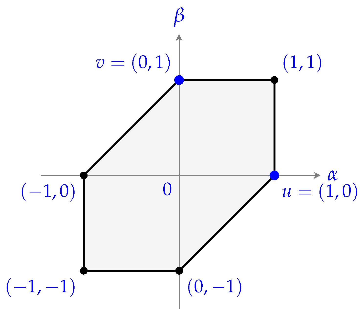
Example 2.

Let $X=({\mathbb{R}}^2,\parallel ·{\parallel }_H)$, where

$${\parallel (\alpha ,\beta )\parallel }_H=\max \left\{\right|\alpha |,|\beta |,|\alpha -\beta \left|\right\}.$$

The corresponding unit sphere is shown in Figure 1.

Then, $S_X$ is an affine regular hexagon. Corollary 7 yields

$$C_2^I\left(X\right)={\displaystyle \frac{5}{4}}.$$

By contrast, the unrestricted constant is strictly larger. Indeed, by (9), $C_2\left(X\right)=C_{\mathrm{NJ}}\left(X\right)$. Take

$$u=(1,0),v=(0,1).$$

Both vectors belong to $S_X$, but they are not isosceles orthogonal, since

$${\parallel u+v\parallel }_H=1,{\parallel u-v\parallel }_H=2.$$

For $0\le \tau \le 1$, we have

$${\parallel u+\tau v\parallel }_H=1,{\parallel u-\tau v\parallel }_H=1+\tau .$$

Hence,

$$C_2\left(X\right)\ge {\displaystyle \frac{M_2{(1,1+\tau )}^2}{1+{\tau }^2}}={\displaystyle \frac{1+{(1+\tau )}^2}{2(1+{\tau }^2)}}=:F\left(\tau \right).$$

A direct differentiation provides

$$F^{\prime }\left(\tau \right)={\displaystyle \frac{1-\tau -{\tau }^2}{{(1+{\tau }^2)}^2}},$$

so F attains its maximum on $[0,1]$ at

$${\tau }_0={\displaystyle \frac{\sqrt{5}-1}{2}}.$$

Substitution yields

$$C_2\left(X\right)\ge F\left({\tau }_0\right)={\displaystyle \frac{3+\sqrt{5}}{4}}>{\displaystyle \frac{5}{4}}=C_2^I\left(X\right).$$

This comparison makes the role of the isosceles restriction explicit. On the same affine regular hexagonal space, the direct constant is $C_2^I\left(X\right)=5/4$, whereas the unrestricted constant admits non-isosceles pairs for which the normalized value is at least $(3+\sqrt{5})/4>5/4$. Thus, the condition $x{\perp }_{I}y$ removes genuinely extremal directions from the unrestricted problem, and the resulting constant records geometric information that is lost when no orthogonality constraint is imposed.

Corollary 8.

Let X be a Radon plane. If $C_{t_0}^I\left(X\right)=5/4$ for one $t_0\in [-\infty ,\infty )$, then

$$C_t^I\left(X\right)={\displaystyle \frac{5}{4}}\mathit{for}\mathit{every}-\infty \le t<\infty .$$

Proof. 

The hypothesis implies, by Theorem 12, that $S_X$ is an affine regular hexagon. The converse part of the same theorem then provides the displayed identity for every t. □

Remark 10.

The sharpness assertions established in the paper have the following scope:

(i)

The universal lower bound $C_t^I\left(X\right)\ge 1$ is attained by Hilbert spaces for every t. The universal upper bound $C_t^I\left(X\right)\le 2$ is attained precisely when $J\left(X\right)=2$, equivalently when X is not uniformly non-square (Theorem 8); ${\mathsf{\ell }}_1^2$ and ${\mathsf{\ell }}_{\infty }^2$ are explicit examples.

(ii)

The lower James bound $C_t^I\left(X\right)\ge J{\left(X\right)}^2/2$ is attained by the classical ${\mathsf{\ell }}_p$ and $L_p[0,1]$ spaces for $t\le 2$ (Theorem 11), and by their cases $p=1,2,\infty$ for all t. The upper James bound is attained by affine regular hexagonal planes for all t, with $J=3/2$ and $C_t^I=5/4$, and by all spaces with $J=2$. These examples establish attainability, not optimality at every prescribed intermediate value of J.

(iii)

In finite dimensions, Theorem 6 provides a necessary and sufficient extremal-pair condition for equality in the upper James bound at $\tau =J\left(X\right)-1$; equality for one order forces equality for all orders. Corollary 3 supplies the corresponding necessary concentration properties of maximizing sequences without a finite-dimensional assumption.

(iv)

Within the class of Radon planes, equality $C_t^I=5/4$ is completely characterized by affine regular hexagonal unit spheres (Theorem 12). No classification of all spaces attaining $C_t^I=1$, or the lower James bound, is asserted here.

To close the section, the preceding calculations produce three simple but useful benchmark profiles, summarized in

Table 1. Benchmark isosceles-orthogonal profiles and constants.

Geometry	${\mathit{J}}_{\mathit{X},\mathit{t}}^{\mathit{I}}\left(\mathit{\tau }\right)$ for $0\le \mathit{\tau }\le 1$	${\mathit{C}}_{\mathit{t}}^{\mathit{I}}\left(\mathit{X}\right)$
Hilbert space	$\sqrt{1+{\tau }^2}$	1
Affine regular hexagonal Radon plane	$1+\tau /2$	$5/4$
${\mathsf{\ell }}_1^2$ or ${\mathsf{\ell }}_{\infty }^2$	$1+\tau$	2

. They describe Euclidean geometry, hexagonal Radon geometry, and the endpoint $J\left(X\right)=2$, respectively.

All three formulas hold for every $-\infty \le t<\infty$. The table also shows that the parameter-independence of an exact profile does not by itself characterize Hilbert space: it may arise because the two deformed chord lengths coincide identically along a suitable extremal isosceles pair.

The exact behavior beyond the quadratic power-mean range remains open for $1<p<\infty$, $p\ne 2$, and leads to the following extremal problem. The numerical exploration in Remark 8 is not a resolution of it.

Problem 1.

Determine the exact values of $C_t^I\left({\mathsf{\ell }}_p\right)$ and $C_t^I\left(L_p[0,1]\right)$ for $t>2$ and $1<p<\infty$, $p\ne 2$. In particular, decide whether

$$C_t^I\left({\mathsf{\ell }}_p\right)=C_t^I\left(L_p[0,1]\right)=\max \{2^{2/p-1},2^{1-2/p}\}$$

continues to hold beyond the range $t\le 2$, or whether a genuine t-dependent transition occurs. For $t>2$, the power mean increasingly favors the larger deformed chord, while the isosceles condition constrains only the undeformed endpoint configuration; thus, a solution appears to require a finer analysis of extremal isosceles pairs under the deformation $x\pm \tau y$.

5. Conclusions

This paper develops a direct isosceles-orthogonal version of the Takahashi–von Neumann–Jordan scale and shows that the orthogonality restriction produces genuinely new geometric information rather than a formal reformulation of the unrestricted theory. The resulting profile and constant are sharply controlled by the James constant, leading to quantitative estimates, stability phenomena, and a characterization of uniform non-squareness. The exactness principle, applied to known classical formulas for $t\le 2$, and the transfer of Mizuguchi’s Radon-plane theorem to the new constants illustrate the sensitivity of the construction to the underlying norm geometry, while the comparison with the unrestricted constant shows that imposing isosceles orthogonality can change the extremal behavior itself. These results provide a systematic connection between isosceles orthogonality, classical geometric constants, and the Takahashi power-mean framework, and indicate that orthogonality-restricted invariants offer a useful perspective on the quantitative geometry of Banach spaces.