Resolution-Adaptive Compact-Support Priors for Bayesian Wavelet Denoising: A Wendland–Semicircle Slab Mixture for Low-SNR Signal Recovery

Abstract

We propose a resolution-adaptive Bayesian wavelet-denoising method for noisy one-dimensional signals. The main contribution is a spike-and-slab prior whose continuous slab is a mixture of a compactly supported Wendland-type polynomial kernel and the semicircle density, with data-adaptive, resolution-specific mixture weights, produced by a low-dimensional empirical-Bayes trend. The Wendland component concentrates mass near zero and vanishes smoothly at the support boundary, whereas the semicircle component is more dispersed. This construction combines explicit sparsity and support control with an interpretable mechanism for adapting the shrinkage shape across resolutions. Under squared-error loss, we derive the posterior-mean estimator; establish key symmetry, boundedness, continuity, and limiting properties; define pointwise fixed-hyperparameter bias, variance, and risk; and develop an empirical-Bayes estimation procedure. The Wendland contribution has finite-sum expressions under a Laplace working likelihood, while the semicircle contribution is evaluated by stable one-dimensional integration. Simulations using the Bumps, Blocks, Doppler, and HeaviSine signals compare the proposed Gaussian- and Laplace-likelihood versions with universal thresholding, false-discovery-rate (FDR) thresholding, cross-validation (CV), Stein’s unbiased risk estimate (SURE), the Bayesian adaptive multiresolution shrinker (BAMS), and a nonlocal-prior (NLP)-based method. In the primary Gaussian-error simulation study, the Gaussian-likelihood version was the strongest non-NLP method in 24 of the 36 design cells, including 11 of the 12 low signal-to-noise ratio (SNR) cells, and had a substantially more favorable computational profile than the Laplace-likelihood version. Analysis of a seismic acceleration trace from the 2008 Chino Hills earthquake illustrates attenuation of rapid fluctuations and preservation of the dominant acceleration event under the chosen diagnostics. Using the processed channel-1 trace as surrogate truth, the corresponding semi-synthetic validation showed that WS–Gaussian improved on the noisy observation at lower and moderate SNRs but not at the highest SNR.

1. Introduction

Wavelet methods provide a localized representation of an unknown function in both the observation and scale domains. This localization is particularly useful for signals containing discontinuities, isolated peaks, sharp transitions, and rapid oscillations. A second important feature is sparsity, which means that, at a given resolution level, most wavelet coefficients are often close to zero, whereas a relatively small number of coefficients describe the principal features of the signal. Wavelet shrinkage exploits this structure by reducing noisy empirical coefficients before reconstructing the signal through the inverse discrete wavelet transform [1,2,3,4]. We propose a Bayesian wavelet-shrinkage model whose continuous slab is a bounded mixture of a compactly supported Wendland-type density and the semicircle density. The model permits the mixture weight and the support scale to vary with resolution, while the extent to which the data identify such variation is assessed empirically.

Classical wavelet estimators include hard and soft thresholding, false-discovery-rate (FDR) thresholding, cross-validation (CV), and Stein’s unbiased risk estimation (SURE) [1,2,5,6]. These procedures are useful and often fast, but their shrinkage behavior is governed by a threshold-selection rule rather than by an explicit prior distribution for the unknown coefficient. Universal hard or soft thresholds can be conservative for moderate signals; hard thresholding also introduces a discontinuous decision at the threshold, whereas soft thresholding imposes a fixed shrinkage bias on retained coefficients. FDR thresholding controls a multiple-testing criterion rather than directly minimizing reconstruction loss, CV can be computationally expensive and sensitive to the validation scheme, and SURE can be variable in low-SNR settings when the estimated risk is noisy. These are not universal failures, but they motivate an explicit prior-based alternative. A Bayesian prior can encode sparsity through a spike at zero, symmetry and bounded support through the slab, and uncertainty about the magnitude of nonzero coefficients through its continuous shape. Early Bayesian wavelet models used mixtures of normal distributions or mixtures involving a point mass at zero and a continuous slab [7,8,9]. Subsequent work considered double-exponential, uniform, double-Weibull, beta, logistic, compact-support, and nonlocal priors [10,11,12,13,14,15,16,17]. Low-signal-to-noise ratio (SNR) settings are particularly challenging because an observed moderate-size coefficient may represent either a genuine local feature or noise. Bayesian shrinkage rules are attractive in this setting because they can incorporate uncertainty about both possibilities [16,18].

Compactly supported slab priors are appealing because their support and shape can control the attenuation of moderate wavelet coefficients and the behavior of the shrinkage rule near the support boundary. The contribution here is the specific Wendland–semicircle bounded mixture slab for Bayesian wavelet coefficient shrinkage, together with a resolution-indexed mixture parameter and a data-adaptive support scale. This is a narrower novelty claim than a claim about Wendland functions, semicircle laws, compact support, or resolution-adaptive sparsity in general. The Wendland component is a normalized compactly supported polynomial density with a high-order zero at the support boundary. Wendland functions were originally introduced as compactly supported positive-definite functions for scattered-data approximation [19,20]. In the present model, this component is concentrated near zero and represents small nonzero coefficients that are difficult to distinguish from noise. The semicircle component is also symmetric and compactly supported, but is more dispersed and places relatively more mass away from zero. The semicircle law is classically associated with the limiting eigenvalue distribution of random matrices [21]; here, it is used as a bounded slab density rather than as a spectral limit. To the best of our knowledge, the particular combination of these two bounded densities as a mixture slab for Bayesian wavelet shrinkage has not previously been studied in this form. Henceforth, we use the abbreviation WS for Wendland–semicircle.

The proposed prior combines the two slab shapes with a point mass at zero. At each resolution level, a mixture weight determines the relative contribution of the Wendland component, while a support-scale parameter determines the common bounded truncation interval for the two slab densities. The weight is parameterized through a low-dimensional empirical-Bayes trend in resolution. Thus, the model permits the relative slab contribution to vary with resolution; whether the data materially identify that variation is examined in the component-and-adaptivity comparison. The prior retains an explicit spike at zero, allows a single specification to express both strong concentration near zero and preservation of moderate coefficients, and maintains an interpretable bounded-support structure. The posterior-mean rule is computationally tractable because the Wendland contribution benefits from its finite polynomial form, whereas the semicircle contribution reduces to a one-dimensional integral. We consider a Gaussian observation model as the primary specification and a Laplace working likelihood as an alternative sensitivity specification.

Our empirical evaluation assesses reconstruction accuracy, normalized error, paired performance, and computational cost. The primary Gaussian-error experiment considers the Bumps, Blocks, Doppler, and HeaviSine test signals at $n=512$, 1024, and 2048, with amplitude SNR values $\rho \in \{0.2,1,3\}$ and 100 replications per design cell. An expanded $n=1024$ experiment additionally uses $\rho \in \{0.5,2,5\}$. WS–Gaussian and WS–Laplace are compared with universal thresholding, FDR thresholding, CV, SURE, the Bayesian adaptive multiresolution shrinker (BAMS), and a nonlocal-prior (NLP)-based method. In the original Gaussian grid, WS–Gaussian is the best non-NLP method in 24 of the 36 cells and in 11 of the 12 low-SNR signal cells. These are cellwise statements rather than claims of universal dominance; pooled and normalized summaries, including the computational cost of the numerical methods, are reported separately.

We also analyze a 77-s, 200 Hz strong-motion accelerogram from the 29 July 2008 Chino Hills earthquake recorded at station 24763. The real-data analysis compares WS fits, the two component-specific endpoint fits, and classical thresholding rules using residual variability, residual roughness, retained squared energy, preservation and timing of the dominant acceleration peak, and waveform plots. Because the observed record has no trusted noise-free reference, these diagnostics describe the amount and character of the modification rather than denoising risk. A separate semi-synthetic validation treats the processed channel-1 trace as a surrogate truth, adds controlled Gaussian noise at prespecified amplitude SNR values, and evaluates recovery against that surrogate. It therefore complements, but does not replace, the real-data illustration.

The remainder of the article is organized as follows. Section 2 introduces the nonparametric regression and wavelet-domain models. Section 3 defines the Wendland and semicircle slab densities and the mixture prior. Section 4 establishes properties of the prior and the resulting shrinkage rule. Section 5 develops posterior inference and the empirical-Bayes fitting procedure. Section 6 presents the simulation design and results, and Section 7 gives the seismic-trace application; the semi-synthetic validation is reported in Supplementary Section S3.2. Section 8 summarizes the findings, limitations, and extensions.

2. Statistical Model and Wavelet Representation

Let $\mathbb{R}$ denote the real line and let $\mathbb{N}=\{1,2,\dots \}$. Let N denote the number of observations in the original record and let $\tilde{N}$ denote the length of the vector supplied to the discrete wavelet transform. In the idealized dyadic setting considered here, $N=\tilde{N}=n=2^J$, where $J\in \mathbb{N}$ is the number of dyadic resolution steps. Suppose that the N observations are collected at equally spaced design points $x_i=(i-1)/(N-1)$, $i=1,\dots ,N$. We observe

$$y_i=f\left(x_i\right)+{ϵ}_i,i=1,\dots ,N,$$

(1)

where $f:[0,1]\to \mathbb{R}$ is an unknown regression function and ${ϵ}_i$ are independent and identically distributed Gaussian errors satisfying

$${ϵ}_i\sim N(0,{\sigma }^2),{\sigma }^2>0,$$

(2)

where ${\sigma }^2$ is the observational noise variance.

Let $\mathbf{x}={(x_1,\dots ,x_N)}^T$, $\mathbf{y}={(y_1,\dots ,y_N)}^T$, $\mathbf{f}={(f\left(x_1\right),\dots ,f\left(x_N\right))}^T$, and $\mathit{ϵ}={({ϵ}_1,\dots ,{ϵ}_N)}^T$. Then, (1) can be written as

$$\mathbf{y}=\mathbf{f}+\mathit{ϵ},\mathit{ϵ}\sim N_N(\mathbf{0},{\sigma }^2{\mathbf{I}}_N),$$

where $N_N$ denotes the N-variate normal distribution and ${\mathbf{I}}_N$ is the $N\times N$ identity matrix.

Let $\varphi$ be a scaling function and let $\psi$ be a mother wavelet generating an orthonormal wavelet basis. For a location index k and resolution level j, define

$${\varphi }_{j,k}\left(x\right)=2^{j/2}\varphi (2^{j}x-k),{\psi }_{j,k}\left(x\right)=2^{j/2}\psi (2^{j}x-k).$$

For a fixed primary resolution level $J_0$, the wavelet expansion of f is written formally as

$$f\left(x\right)=\sum _k{c}_{J_0,k}{\varphi }_{J_0,k}\left(x\right)+{\displaystyle \sum _{j=J_0}^{\infty }}\sum _k{\theta }_{j,k}{\psi }_{j,k}\left(x\right),{\theta }_{j,k}={\int }_0^{1}f\left(x\right){\psi }_{j,k}\left(x\right)dx,$$

where $c_{J_0,k}$ are scaling coefficients and ${\theta }_{j,k}$ are detail wavelet coefficients. In the finite-sample analysis below, only levels $j=J_0,\dots ,J-1$ are represented, and the scaling coefficients are retained without shrinkage.

Let $\mathcal{P}:{\mathbb{R}}^N\to {\mathbb{R}}^{\tilde{N}}$ denote a prescribed deterministic padding or extension operator, where $\tilde{N}=2^J$. Define the vectors supplied to the DWT by

$$\tilde{\mathbf{y}}=\mathcal{P}\left(\mathbf{y}\right),\tilde{\mathbf{f}}=\mathcal{P}\left(\mathbf{f}\right),\widetilde{\mathit{ϵ}}=\mathcal{P}\left(\mathit{ϵ}\right).$$

Thus, $\tilde{\mathbf{y}}=\tilde{\mathbf{f}}+\widetilde{\mathit{ϵ}}$. In the ideal dyadic setting, $\mathcal{P}$ is the identity and $N=\tilde{N}$. For a padded record, $\tilde{\mathbf{y}}$ is the computational DWT input. The padding does not represent additional independent observations. In particular, when $\mathcal{P}$ is not the identity, $\widetilde{\mathit{ϵ}}$ need not have independent coordinates. For a non-dyadic record, the discrete wavelet transform is applied after a documented extension to a dyadic length $\tilde{N}\ge N$, and the reconstructed values are truncated to the original N observations before reporting application-level diagnostics. The specific extension rule used for the seismic record is given in Section 7.

Let $\mathbf{W}$ be an orthogonal $\tilde{N}\times \tilde{N}$ matrix representing a DWT, so that ${\mathbf{W}}^T\mathbf{W}={\mathbf{I}}_{\tilde{N}}$. For each detail level $j=J_0,\dots ,J-1$, define the observed and true detail-coefficient vectors by ${\mathbf{d}}_j={(d_{j,k}:k\in {\mathcal{K}}_j)}^T$ and ${\mathit{\theta }}_j={({\theta }_{j,k}:k\in {\mathcal{K}}_j)}^T$, respectively. Let ${\mathbf{c}}_{J_0}^{\left(y\right)}$ and ${\mathbf{c}}_{J_0}^{\left(f\right)}$ denote the observed and true scaling-coefficient vectors at the primary resolution level. With the DWT coefficients ordered by placing the scaling coefficients first, define

$$\mathbf{d}=\mathbf{W}\tilde{\mathbf{y}}=\left(\begin{array}{c}{\mathbf{c}}_{J_0}^{\left(y\right)}\\ {\mathbf{d}}_{J_0}\\ ⋮\\ {\mathbf{d}}_{J-1}\end{array}\right),\mathit{\theta }=\mathbf{W}\tilde{\mathbf{f}}=\left(\begin{array}{c}{\mathbf{c}}_{J_0}^{\left(f\right)}\\ {\mathit{\theta }}_{J_0}\\ ⋮\\ {\mathit{\theta }}_{J-1}\end{array}\right),{\mathit{ϵ}}^{*}=\mathbf{W}\widetilde{\mathit{ϵ}}.$$

Thus, $\mathbf{d}$, $\mathit{\theta }$, and ${\mathit{ϵ}}^{*}$ are $\tilde{N}$-dimensional vectors. In the ideal dyadic setting,

$${\mathit{ϵ}}^{*}\sim N_{\tilde{N}}(\mathbf{0},{\sigma }^2{\mathbf{I}}_{\tilde{N}}).$$

For a nontrivial padding operator, no independent multivariate-normal assertion is made for ${\mathit{ϵ}}^{*}$. The coefficientwise model below is used as the working likelihood for the padded analysis.

The prior in (10), below, is assigned only to the scalar detail coefficients ${\theta }_{j,k}$; the scaling coefficients ${\mathbf{c}}_{J_0}^{\left(f\right)}$ are retained without shrinkage. In scalar expressions below, $\theta$ denotes a generic value of a detail coefficient, whereas ${\theta }_{j,k}$ denotes the particular detail coefficient at level j and location k. For a detail coefficient at level j and location k, the coefficientwise wavelet-domain model is

$$d_{j,k}={\theta }_{j,k}+{ϵ}_{j,k}^{*},{ϵ}_{j,k}^{*}\sim N(0,{\sigma }^2),$$

(3)

where $j=J_0,\dots ,J-1$ and $k\in {\mathcal{K}}_j=\{0,1,\dots ,2^j-1\}$. Here, $d_{j,k}$ is the observed empirical detail coefficient.

3. Adaptive Wendland–Semicircle Prior

3.1. Two Normalized Slab Densities

For a set $A\subseteq \mathbb{R}$, let $I\left(A\right)$ denote its indicator function. Let u be a dimensionless coefficient and let $\beta >0$ be a scale parameter. We define the Wendland-type kernel

$$K_W\left(u\right)={\displaystyle \frac{3}{2}}{(1-|u\left|\right)}^4(1+4|u\left|\right)I\left(\right|u|<1).$$

(4)

The polynomial in (4) can equivalently be written, for $\left|u\right|<1$, as

$${(1-|u\left|\right)}^4(1+4|u\left|\right)={1-10\left|u\right|}^2+{20\left|u\right|}^3-{15\left|u\right|}^4+4{\left|u\right|}^5.$$

(5)

The normalization follows from

$${\int }_{-1}^1{K}_W\left(u\right)du=3{\int }_0^1{(1-u)}^4(1+4u)du=1.$$

(6)

The second slab is the semicircle kernel

$$K_S\left(u\right)={\displaystyle \frac{2}{\pi }}\sqrt{1-u^2}I\left(\right|u|<1).$$

(7)

Since ${\int }_{-1}^1\sqrt{1-u^2}du=\pi /2$, $K_S$ is also a density. The scale versions of these kernels are

$$\begin{array}{cc}\hfill g_W(\theta ;\beta )& ={\displaystyle \frac{1}{\beta }}{K}_W\left({\displaystyle \frac{\theta }{\beta }}\right)={\displaystyle \frac{3}{2\beta }}{\left(1-{\displaystyle \frac{\left|\theta \right|}{\beta }}\right)}^4\left(1+4{\displaystyle \frac{\left|\theta \right|}{\beta }}\right)I\left(\right|\theta |<\beta ),\hfill \\ \hfill g_S(\theta ;\beta )& ={\displaystyle \frac{1}{\beta }}{K}_S\left({\displaystyle \frac{\theta }{\beta }}\right)={\displaystyle \frac{2}{\pi {\beta }^2}}\sqrt{{\beta }^2-{\theta }^2}I\left(\right|\theta |<\beta ).\hfill \end{array}$$

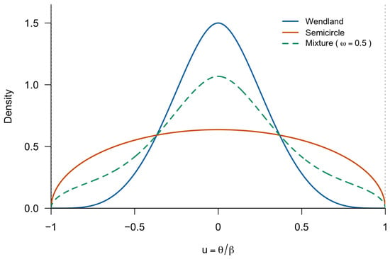
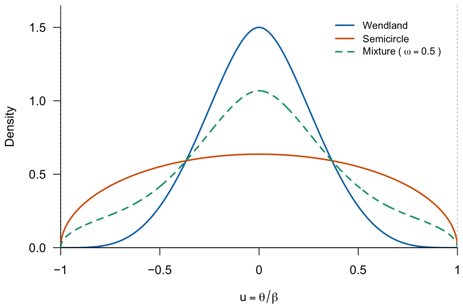
Both densities are symmetric about zero and have support $[-\beta ,\beta ]$. The Wendland density is more concentrated near zero and has a high-order zero at the support boundary. The semicircle density is less concentrated at the center and allocates relatively more prior mass to moderate coefficients. The differing concentration and dispersion of the two slab densities are illustrated in Figure 1, which also displays their equal-weight continuous mixture on the standardized support.

Figure 1. Normalized Wendland-type and semicircle slab densities on the common standardized support $u=\theta /\beta$, together with their continuous equal-weight mixture $0.5K_W\left(u\right)+0.5K_S\left(u\right)$. The mixture curve is shown for illustration only. In the proposed model, the mixture weight ${\omega }_j$ is estimated separately at each resolution level. The point-mass spike at zero is not shown.

Proposition 1 

(Normalization and dispersion). For every $\beta >0$, $g_W(·;\beta )$ and $g_S(·;\beta )$ are probability densities on $\mathbb{R}$, both have mean zero, and

$${Var}_W\left(\theta \right)={\displaystyle \frac{{\beta }^2}{14}},{Var}_S\left(\theta \right)={\displaystyle \frac{{\beta }^2}{4}}.$$

(8)

Proof. 

Normalization and symmetry follow from (6) and the semicircle-area formula. For the Wendland density, using symmetry and (5),

$$\begin{array}{c}{E}_W\left({\theta }^2\right)=3{\beta }^2{\int }_0^1{u}^2{(1-u)}^4(1+4u)du={\displaystyle \frac{{\beta }^2}{14}}.\end{array}$$

For the semicircle density,

$$\begin{array}{c}{E}_S\left({\theta }^2\right)={\displaystyle \frac{2{\beta }^2}{\pi }}{\int }_{-1}^1{u}^2\sqrt{1-u^2}du={\displaystyle \frac{{\beta }^2}{4}}.\end{array}$$

The means are zero by symmetry, so the second moments equal the variances.    □

3.2. Spike-and-Mixture Slab Prior

Let ${\delta }_0$ denote the Dirac probability measure concentrated at zero. For each resolution level j, let ${\pi }_j\in (0,1)$ be the prior probability that a coefficient is exactly zero, let ${\omega }_j\in [0,1]$ be the conditional probability of the Wendland component given that the coefficient is nonzero, and let ${\beta }_j>0$ be the level-specific support scale. Define the continuous mixture slab

$$g_j(\theta ;{\omega }_j,{\beta }_j)={\omega }_j{g}_W(\theta ;{\beta }_j)+(1-{\omega }_j)g_S(\theta ;{\beta }_j).$$

(9)

The proposed prior for a detail coefficient is

$${\theta }_{j,k}\mid {\pi }_j,{\omega }_j,{\beta }_j\sim {\pi }_j{\delta }_0+(1-{\pi }_j)g_j(\theta ;{\omega }_j,{\beta }_j).$$

(10)

The main theoretical development considers the interior mixture case $0<{\omega }_j<1$, in which both slab components receive positive prior weight. The endpoint values define reduced one-component models:

$$g_j(\theta ;1,{\beta }_j)=g_W(\theta ;{\beta }_j),g_j(\theta ;0,{\beta }_j)=g_S(\theta ;{\beta }_j).$$

Thus, ${\omega }_j=1$ is the Wendland-only specification and ${\omega }_j=0$ is the Semicircle-only specification. These endpoint specifications are fitted separately in the component-and-adaptivity comparison. They are also used in the numerical endpoint checks, where the absent component is omitted rather than evaluated with a zero numerical weight.

Equivalently, introduce a latent component indicator $Z_{j,k}\in \{0,W,S\}$, where $Z_{j,k}=0$ denotes the spike, $Z_{j,k}=W$ denotes the Wendland slab, and $Z_{j,k}=S$ denotes the semicircle slab. Its prior probabilities are

$$Pr(Z_{j,k}=0)={\pi }_j,Pr(Z_{j,k}=W)=(1-{\pi }_j){\omega }_j,Pr(Z_{j,k}=S)=(1-{\pi }_j)(1-{\omega }_j).$$

Conditional on $Z_{j,k}=0$, ${\theta }_{j,k}=0$. Conditional on $Z_{j,k}=W$ or $Z_{j,k}=S$, the coefficient has density $g_W(·;{\beta }_j)$ or $g_S(·;{\beta }_j)$, respectively.

The prior variance of a nonzero coefficient at level j is

$$Var({\theta }_{j,k}\mid Z_{j,k}\ne 0)={\beta }_j^2\left\{{\displaystyle \frac{{\omega }_j}{14}}+{\displaystyle \frac{1-{\omega }_j}{4}}\right\},$$

(11)

which also applies to the two endpoint models. The prior variance of a nonzero coefficient at level j is given by (11), and the unconditional prior variance is $(1-{\pi }_j)$ times that quantity. Thus, ${\pi }_j$ controls sparsity, ${\beta }_j$ controls the coefficient scale, and ${\omega }_j$ controls the shape of the nonzero slab. The endpoint values ${\omega }_j=0$ and ${\omega }_j=1$ are handled by the corresponding one-component posterior formulas.

3.3. Resolution-Dependent Hyperparameters

Following the principle that fine-scale coefficients are more likely to be noise, we use the level-dependent spike probability:

$${\pi }_j=1-{\displaystyle \frac{1}{{(j-J_0+\ell )}^{\gamma }}},j=J_0,\dots ,J-1,$$

(12)

where $\ell >1$ is the spike-offset parameter and $\gamma >0$ is the resolution sparsity exponent. Larger values of $\gamma$ make the spike probability increase more rapidly with resolution level, whereas ℓ controls its starting value. These quantities are fixed in the primary analysis and are varied one at a time in the supplementary sensitivity study.

To adapt the slab shape across resolution levels, define

$$t_j={\displaystyle \frac{j-J_0}{J-1-J_0}},\mathit{\eta }={({\eta }_0,{\eta }_1)}^T\in {\mathbb{R}}^2,$$

for $J>J_0+1$, and set

$${\omega }_j\left(\mathit{\eta }\right)={logit}^{-1}({\eta }_0+{\eta }_1{t}_j)={\displaystyle \frac{exp({\eta }_0+{\eta }_1{t}_j)}{1+exp({\eta }_0+{\eta }_1{t}_j)}}.$$

(13)

Here, ${\eta }_0$ controls the Wendland weight at the coarsest detail level and ${\eta }_1$ controls its change across resolution levels. A positive ${\eta }_1$ describes an increasing fitted Wendland weight under this parameterization; it does not imply that such an increase is present in every dataset. If no trend is desired, setting ${\eta }_1=0$ yields a common slab mixture weight across levels. The fitted weights and their empirical identification are assessed in the component-and-adaptivity analysis.

The scale ${\beta }_j$ defines the common prior truncation interval, but its fitted value is treated as a data-adaptive truncation-scale choice rather than as a formal estimator of an unknown true support. It may be specified from prior knowledge or selected from the empirical coefficients. We recommend the robust upper-quantile rule

$${\widehat{\beta }}_j^{\left(0\right)}=max\left\{\widehat{\sigma },Q_{\varkappa }\left(\left\{\right|d_{j,k}|:k\in {\mathcal{K}}_j\}\right)\right\},\varkappa \in (0,1),$$

(14)

where $Q_{\varkappa }$ denotes the empirical $\varkappa$-quantile and $\widehat{\sigma }$ is the robust noise-scale estimate defined in Section 5. To ensure compatibility with the assumption ${\beta }_j>0$, define

$$s_{\beta }=max\left\{1,\widehat{\sigma },\underset{\ell ,k}{max}\left|d_{\ell ,k}\right|\right\},{\beta }_{min}={\epsilon }_{\beta }{s}_{\beta },$$

where the maximum is taken over all detail levels and locations, and ${\epsilon }_{\beta }>0$ is a small numerical constant. We use ${\epsilon }_{\beta }={10}^{-8}$. The fitted support scale is therefore

$${\widehat{\beta }}_j=max\left\{{\widehat{\beta }}_j^{\left(0\right)},{\beta }_{min}\right\}.$$

(15)

In the implementation, $Q_{\varkappa }$ is the empirical quantile calculated by the exact quantile convention used in the R analysis (the default stats::quantile type 7 if unchanged). The value $\varkappa =0.99$ is therefore a data-adaptive truncation rule, not a formal estimator or guarantee of the true support. At coarse resolutions, relatively few coefficients determine this quantile, and a future coefficient may exceed the fitted interval. This floor preserves ${\widehat{\beta }}_j\ge \widehat{\sigma }$ while preventing a degenerate zero support when $\widehat{\sigma }=0$ and all relevant coefficients vanish. The alternative ${\widehat{\beta }}_j={max}_{k\in {\mathcal{K}}_j}\left|d_{j,k}\right|$ can be used when a conservative truncation scale is preferred, but it is more sensitive to isolated noise outliers and must likewise be subject to the positive floor in (15). The default hyperparameter choices and their interpretations are summarized in Table 1. These settings are used throughout the primary simulation and real-data analyses unless a sensitivity analysis is explicitly identified.

Table 1. Default prior hyperparameters and likelihood-specific tuning quantities.

Quantity	Default	Interpretation
$J_0$	0	Primary detail resolution level
ℓ	2	Spike-offset parameter controlling the initial spike probability
$\gamma$	$2.4$	Controls the increase of sparsity with resolution
$\varkappa$	$0.99$	Quantile used for ${\widehat{\beta }}_j$
$\widehat{\sigma }$	Equation (36)	Robust noise-scale estimate used in both likelihood versions
$\lambda$	$1/\left(2{\widehat{\sigma }}^2\right)$	Rate for the Laplace working likelihood

4. Bayesian Shrinkage Rule and Its Properties

Unless stated otherwise, all theoretical results in this section condition on fixed values of the prior and likelihood hyperparameters. Thus, the propositions describe the fixed-hyperparameter, or oracle, rule ${\delta }_j(d;{\pi }_j,{\omega }_j,{\beta }_j,\lambda )$. The effect of estimating these quantities from the observed wavelet coefficients is treated separately in Section 5.

4.1. Gaussian Likelihood Formulation

Under (3), the coefficientwise likelihood is

$$L_N(d\mid \theta ,{\sigma }^2)={\displaystyle \frac{1}{\sqrt{2\pi {\sigma }^2}}}exp\left\{-{\displaystyle \frac{{(d-\theta )}^2}{2{\sigma }^2}}\right\}.$$

(16)

For any nonnegative likelihood $L(d\mid \theta )$, define the mixture-slab moments

$$M_{r,j}\left(d\right)={\int }_{-{\beta }_j}^{{\beta }_j}{\theta }^r{g}_j(\theta ;{\omega }_j,{\beta }_j)L(d\mid \theta )d\theta ,r\in \{0,1\}.$$

The corresponding component moments are

$$\begin{array}{c}{M}_{r,W,j}\left(d\right)={\int }_{-{\beta }_j}^{{\beta }_j}{\theta }^r{g}_W(\theta ;{\beta }_j)L(d\mid \theta )d\theta ,\\ M_{r,S,j}\left(d\right)={\int }_{-{\beta }_j}^{{\beta }_j}{\theta }^r{g}_S(\theta ;{\beta }_j)L(d\mid \theta )d\theta .\end{array}$$

By (9),

$$M_{r,j}\left(d\right)={\omega }_j{M}_{r,W,j}\left(d\right)+(1-{\omega }_j)M_{r,S,j}\left(d\right).$$

Proposition 2 

(Posterior-mean shrinkage rule). Under squared-error loss $L_2(a,\theta )={(a-\theta )}^2$, the Bayes estimator of ${\theta }_{j,k}$ based on $d_{j,k}=d$ is

$${\delta }_j\left(d\right)={\displaystyle \frac{(1-{\pi }_j)M_{1,j}\left(d\right)}{{\pi }_{j}L(d\mid 0)+(1-{\pi }_j)M_{0,j}\left(d\right)}}.$$

(17)

The posterior probabilities of the three latent components are

$$\begin{array}{cc}\hfill p_{0,j}\left(d\right)& ={\displaystyle \frac{{\pi }_{j}L(d\mid 0)}{D_j\left(d\right)}},\hfill \end{array}$$

(18)

$$\begin{array}{cc}\hfill p_{W,j}\left(d\right)& ={\displaystyle \frac{(1-{\pi }_j){\omega }_j{M}_{0,W,j}\left(d\right)}{D_j\left(d\right)}},\hfill \end{array}$$

(19)

$$\begin{array}{cc}\hfill p_{S,j}\left(d\right)& ={\displaystyle \frac{(1-{\pi }_j)(1-{\omega }_j)M_{0,S,j}\left(d\right)}{D_j\left(d\right)}},\hfill \end{array}$$

(20)

where

$$D_j\left(d\right)={\pi }_{j}L(d\mid 0)+(1-{\pi }_j)M_{0,j}\left(d\right).$$

(21)

Consequently,

$${\delta }_j\left(d\right)=p_{W,j}\left(d\right){\mu }_{W,j}\left(d\right)+p_{S,j}\left(d\right){\mu }_{S,j}\left(d\right),$$

(22)

where ${\mu }_{W,j}\left(d\right)=M_{1,W,j}\left(d\right)/M_{0,W,j}\left(d\right)$ and ${\mu }_{S,j}\left(d\right)=M_{1,S,j}\left(d\right)/M_{0,S,j}\left(d\right)$ are the posterior means conditional on the corresponding continuous component.

Proof. 

The marginal likelihood of d is $D_j\left(d\right)$. The spike contributes zero to the posterior first moment, while the continuous mixture contributes $(1-{\pi }_j)M_{1,j}\left(d\right)$. Dividing the posterior first moment by the marginal likelihood gives (17). The component probabilities follow by Bayes’ theorem, and (22) follows by separating the two continuous components.    □

Remark 1. 

Under squared-error loss, the proposed estimator is generally a continuous shrinkage rule rather than an exact hard threshold, so, except at $d=0$, the posterior mean is usually nonzero even though the posterior assigns positive probability to the exact spike. The quantity $p_{0,j}\left(d\right)$ is the appropriate posterior measure of evidence for an exactly zero coefficient.

Proposition 3 

(Continuity of moments and shrinkage rule). Assume that $0<{\pi }_j<1$, ${\beta }_j>0$, and that the prior slab is supported on $[-{\beta }_j,{\beta }_j]$. For either the Gaussian likelihood in (16) with fixed ${\sigma }^2>0$, or the fixed-rate Laplace likelihood in (24) with fixed $\lambda >0$, the functions $M_{r,j}\left(d\right)$, $M_{r,W,j}\left(d\right)$, and $M_{r,S,j}\left(d\right)$ are continuous in d for $r\in \{0,1\}$. Moreover, $D_j\left(d\right)$ is continuous and strictly positive for every $d\in \mathbb{R}$, and the posterior-mean rule ${\delta }_j\left(d\right)$ in (17) is continuous on $\mathbb{R}$.

Proof. 

Fix $d_0\in \mathbb{R}$ and let $d\to d_0$. For either likelihood, the function $L(d\mid \theta )$ is continuous in d for every $\theta$, and it is bounded uniformly over d and $\theta$ by a finite constant that depends only on the fixed likelihood parameter. Since $\left|\theta \right|\le {\beta }_j$ on the slab support, for $r\in \{0,1\}$ the integrands defining the moments are dominated by an integrable function proportional to ${\beta }_j^r{g}_j(\theta ;{\omega }_j,{\beta }_j)$. Dominated convergence therefore gives continuity of $M_{r,j}\left(d\right)$. The same argument applies separately to the Wendland and semicircle moments.

The likelihood is strictly positive at $\theta =0$, and ${\pi }_j>0$, so $D_j\left(d\right)\ge {\pi }_{j}L(d\mid 0)>0$ for every finite d. Hence, the numerator and denominator in (17) are continuous and the denominator never vanishes. Their quotient, ${\delta }_j\left(d\right)$, is consequently continuous on $\mathbb{R}$.    □

Proposition 4 

(Monotonicity of the fixed Gaussian shrinkage rule). Assume the Gaussian likelihood in (16) with fixed ${\sigma }^2>0$, and hold ${\pi }_j$, ${\omega }_j$, and ${\beta }_j$ fixed. Let

$$m_j\left(d\right)={\pi }_j{L}_N(d\mid 0,{\sigma }^2)+(1-{\pi }_j)M_{0,j}^{\left(N\right)}\left(d\right)$$

denote the marginal density of d. Then,

$${\delta }_j\left(d\right)=d+{\sigma }^2{\displaystyle \frac{d}{dd}}log{m}_j\left(d\right),{\delta }_j^{\prime }\left(d\right)={\displaystyle \frac{Var({\theta }_{j,k}\mid d)}{{\sigma }^2}}\ge 0.$$

Consequently, the posterior-mean map is nondecreasing in d for fixed hyperparameters. This conclusion concerns the fixed-hyperparameter rule; it does not by itself establish monotonicity of an empirical-Bayes map whose fitted hyperparameters change with the complete coefficient vector.

Proof. 

For the Gaussian likelihood,

$${\displaystyle \frac{d}{dd}}log{m}_j\left(d\right)={\displaystyle \frac{\mathbb{E}({\theta }_{j,k}\mid d)-d}{{\sigma }^2}}.$$

Consequently, ${\delta }_j\left(d\right)=d+{\sigma }^2{(log{m}_j)}^{\prime }\left(d\right)$. Differentiating the posterior mean under the integral sign gives

$${\delta }_j^{\prime }\left(d\right)=Cov\left({\theta }_{j,k},{\displaystyle \frac{{\theta }_{j,k}-d}{{\sigma }^2}}|d\right)={\displaystyle \frac{Var({\theta }_{j,k}\mid d)}{{\sigma }^2}}\ge 0.$$

The calculation holds for fixed hyperparameters. It does not apply directly to an empirical-Bayes map after $\widehat{\mathit{\eta }}$, ${\widehat{\beta }}_j$, or $\widehat{\sigma }$ has been refitted as a function of the complete observed coefficient vector.    □

Remark 2 

(Endpoint cases). If ${\pi }_j=1$, the prior is degenerate at zero and ${\delta }_j\left(d\right)=0$ for every d; ${\omega }_j$ and ${\beta }_j$ are irrelevant. If ${\pi }_j=0$, the spike is absent and

$${\delta }_j\left(d\right)={\displaystyle \frac{M_{1,j}\left(d\right)}{M_{0,j}\left(d\right)}}.$$

If ${\omega }_j=1$ or ${\omega }_j=0$, the absent semicircle or Wendland component is omitted, respectively. These endpoint formulas are used in the component-specific fits and in the numerical checks.

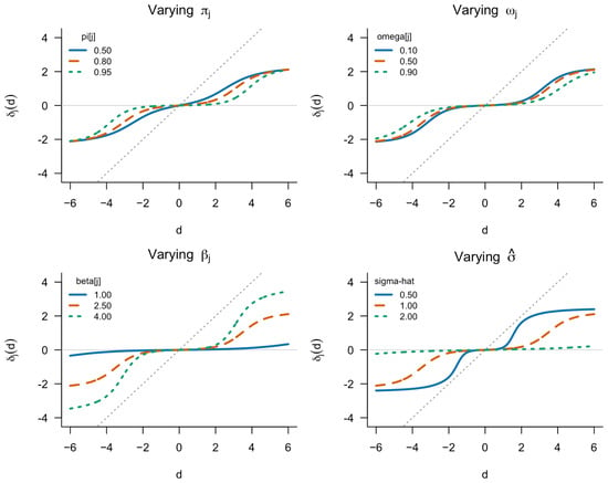
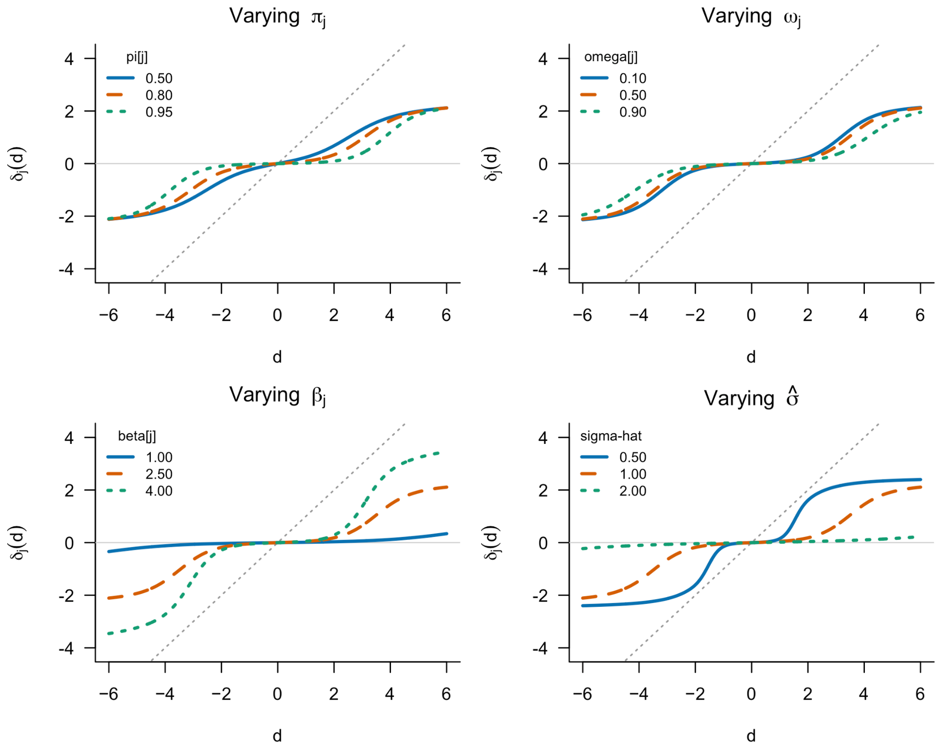
Proposition 3 establishes continuity of the component moments, the posterior denominator, and the resulting shrinkage rule for both likelihood specifications. Figure 2 illustrates how the posterior-mean shrinkage rule changes with the prior spike probability, the Wendland mixture weight, the support scale, and the estimated noise level under the Gaussian likelihood. The plots also show the resulting attenuation relative to the unshrunk rule.

Figure 2. Posterior-mean shrinkage curves ${\delta }_j\left(d\right)$ for the proposed Wendland–semicircle prior under a Gaussian likelihood. Each panel varies one parameter while holding the others fixed: the prior spike probability ${\pi }_j$, the Wendland mixture weight ${\omega }_j$, the slab support scale ${\beta }_j$, and the noise-scale estimate $\widehat{\sigma }$. The gray diagonal line represents the unshrunk rule ${\delta }_j\left(d\right)=d$.

The differences among the panels have distinct interpretations. Increasing ${\pi }_j$ increases the prior probability of the spike at zero and therefore strengthens shrinkage toward zero. Increasing ${\omega }_j$ gives more weight to the Wendland slab, which is more concentrated near zero and vanishes at the support boundary. Relative to the more dispersed semicircle slab, this generally produces greater attenuation of moderate coefficients. Increasing ${\beta }_j$ widens the admissible slab support and delays boundary saturation, allowing larger posterior means when the data support them. Increasing $\widehat{\sigma }$ makes a fixed observed coefficient less informative relative to the noise and therefore increases shrinkage. For small $\left|d\right|$, all curves remain close to zero because the spike is plausible; as $\left|d\right|$ increases, the posterior probability of the slab increases and the curves move toward the diagonal. The curves are odd because the slab and likelihood are symmetric, and the bounded slab prevents the posterior mean from exceeding the fitted support in magnitude.

4.2. Laplace Working Likelihood and Analytic Wendland Contribution

The normal likelihood in (16) is the primary observation model. For a closed-form coefficientwise rule, we also consider the variance-mixture working likelihood used in related Bayesian wavelet-shrinkage constructions. Specifically, let $v>0$ denote a coefficientwise latent variance and suppose

$$d\mid \theta ,v\sim N(\theta ,v),v\sim Exp\left(\lambda \right),\lambda >0,$$

(23)

where $Exp\left(\lambda \right)$ denotes the exponential distribution with density

$$p(v\mid \lambda )=\lambda exp(-\lambda v)I(v>0),\lambda >0.$$

Thus, $\lambda$ is the rate of the exponential distribution assigned to the latent variance v; it is not the Gaussian noise variance ${\sigma }^2$. Integrating out v gives

$$L_L(d\mid \theta ,\lambda )={\displaystyle \frac{a}{2}}exp\{-a|d-\theta \left|\right\},a=\sqrt{2\lambda },$$

(24)

which is the density of a Laplace distribution centered at $\theta$ with scale $1/a$. The parameter $\lambda$ is relevant only to the Laplace working likelihood. In the empirical-Bayes implementation, $\lambda$ is fixed at the value in (37) and is not re-estimated. The numerical safeguard for a zero median absolute deviation (MAD) is described in the noise-scale subsection. The Laplace construction is therefore used as a coefficientwise working likelihood when the data are generated under the Gaussian model (2). The use of (23) should be interpreted as a coefficientwise working likelihood when the original data are generated under the common-variance Gaussian model (2).

For the Laplace likelihood, define the elementary exponential moment:

$${\mathcal{I}}_m(b;u,v)={\int }_u^v{t}^m{e}^{bt}dt,m\in \{0,1,2,\dots \},b\ne 0,u<v.$$

It has the finite-sum representation

$${\mathcal{I}}_m(b;u,v)={\left[e^{bt}{\displaystyle \sum _{r=0}^m}{\displaystyle \frac{{(-1)}^{r}m!}{(m-r)!}}{\displaystyle \frac{t^{m-r}}{b^{r+1}}}\right]}_{t=u}^{t=v}.$$

(25)

For a fixed d, let $\mathcal{P}(d,\beta )$ be the partition of $[-\beta ,\beta ]$ obtained by inserting the points 0 and d whenever they lie strictly inside the interval. On every interval $I=[u_I,v_I]\in \mathcal{P}(d,\beta )$, define $s_{\theta ,I}\in \{-1,1\}$ as the constant sign of $\theta$ on the interior of I, and define $s_{d,I}\in \{-1,1\}$ as the constant sign of $d-\theta$ on the interior of I. Values at partition points are irrelevant because they have Lebesgue measure zero. Let

$$(c_0,c_1,c_2,c_3,c_4,c_5)=(1,0,-10,20,-15,4).$$

Proposition 5 

(Finite-sum Wendland moments). Under the Laplace likelihood (24), for $r\in \{0,1\}$,

$$\begin{array}{cc}\hfill M_{r,W}(d;\beta ,\lambda )=& {\displaystyle \frac{3a}{4\beta }}\sum _{I=[u_I,v_I]\in \mathcal{P}(d,\beta )}{e}^{-a{s}_{d,I}d}{\displaystyle \sum _{m=0}^5}{c}_m{\beta }^{-m}{s}_{\theta ,I}^m{\mathcal{I}}_{r+m}(a{s}_{d,I};u_I,v_I),\hfill \end{array}$$

(26)

where $a=\sqrt{2\lambda }$ and ${\mathcal{I}}_m$ is given by (25). Thus, both the zero-order marginal contribution and the first-order posterior numerator for the Wendland component are available without numerical integration.

Proof. 

By (5), the Wendland density on each interval of the partition is

$$g_W(\theta ;\beta )={\displaystyle \frac{3}{2\beta }}{\displaystyle \sum _{m=0}^5}{c}_m{\beta }^{-m}{s}_{\theta ,I}^m{\theta }^m.$$

On the same interval, $|d-\theta |=s_{d,I}(d-\theta )$, and hence

$$exp\{-a|d-\theta \left|\right\}=e^{-a{s}_{d,I}d}{e}^{a{s}_{d,I}\theta }.$$

Multiplication by ${\theta }^r(a/2)$ and integration over each interval gives (26).    □

For the semicircle component, the substitution $\theta =\beta cost$, $0\le t\le \pi$, yields the stable one-dimensional representation

$$M_{r,S}(d;\beta ,\lambda )={\displaystyle \frac{a}{\pi }}{\int }_0^{\pi }{(\beta cost)}^{r}exp\{-a|d-\beta cost\left|\right\}{sin}^2\left(t\right)dt,r\in \{0,1\}.$$

(27)

For $\left|d\right|\ge \beta$, the integrand has no interior kink. The treatment of the $\left|d\right|<\beta$ case is specified in the numerical implementation paragraph below. Standard adaptive Gauss–Legendre quadrature provides a deterministic and accurate evaluation.

In our implementation, we use several numerical safeguards. In the finite-sum Wendland calculation, the case $\left|b\right|<{10}^{-10}$ is evaluated by the limiting polynomial integral ${\mathcal{I}}_m(0;u,v)=(v^{m+1}-u^{m+1})/(m+1)$, avoiding the powers of $b^{-1}$. Otherwise, the finite-sum expression in (25) is used. If it is non-finite, the code falls back to adaptive integration with relative tolerance ${10}^{-10}$ and absolute tolerance ${10}^{-12}$. Quadrature-based component moments are evaluated on the log scale using row-wise log-sum-exp calculations. The semicircle integral is split at $t_d=arccos(d/\beta )$ when the absolute-value kink is inside the integration interval. The independent quadrature study selected $q=128$ for the remaining simulation-suite analyses. The real-data and semi-synthetic seismic analyses used $q=48$, as specified in Section 7; these orders were fixed before evaluating the corresponding outcomes. The selected orders were not chosen by inspecting the corresponding reconstruction results.

4.3. Structural Properties of the Shrinkage Rule

Proposition 6 

(Symmetry, boundedness, and tail behavior). Consider the prior in (10), where $0<{\pi }_j<1$, ${\beta }_j>0$, and $g_j(·;{\omega }_j,{\beta }_j)$ is a symmetric probability density supported on $[-{\beta }_j,{\beta }_j]$. Assume that the likelihood is finite and strictly positive for finite d and θ, and satisfies $L(-d\mid -\theta )=L(d\mid \theta )$. Then:

(i) 

${\delta }_j(-d)=-{\delta }_j\left(d\right)$ for every $d\in \mathbb{R}$, and ${\delta }_j\left(0\right)=0$;

(ii) 

$|{\delta }_j\left(d\right)|<{\beta }_j$ for every finite d, and $|{\delta }_j\left(d\right)|\le {\beta }_j$ for all d;

(iii) 

If $L=L_N$ is the Gaussian likelihood in (16) with fixed ${\sigma }^2>0$, and $g_j(\theta ;{\omega }_j,{\beta }_j)>0$ for every $\theta \in (-{\beta }_j,{\beta }_j)$, then

$$\underset{d\to \infty }{lim}{\delta }_j\left(d\right)={\beta }_j,\underset{d\to -\infty }{lim}{\delta }_j\left(d\right)=-{\beta }_j;$$

These endpoint values are limits of the posterior mean and are not attained at finite d;

(iv) 

If $L=L_L$ is the fixed-rate Laplace likelihood in (24), with $a>0$, then the tail limits are

$$\underset{d\to \infty }{lim}{\delta }_j\left(d\right)={\displaystyle \frac{(1-{\pi }_j)A_{1,j}^{+}}{{\pi }_j+(1-{\pi }_j)A_{0,j}^{+}}},\underset{d\to -\infty }{lim}{\delta }_j\left(d\right)={\displaystyle \frac{(1-{\pi }_j)A_{1,j}^{-}}{{\pi }_j+(1-{\pi }_j)A_{0,j}^{-}}},$$

where

$$A_{r,j}^{+}={\int }_{-{\beta }_j}^{{\beta }_j}{\theta }^r{g}_j(\theta ;{\omega }_j,{\beta }_j)e^{a\theta }d\theta ,A_{r,j}^{-}={\int }_{-{\beta }_j}^{{\beta }_j}{\theta }^r{g}_j(\theta ;{\omega }_j,{\beta }_j)e^{-a\theta }d\theta ,r\in \{0,1\};$$

(v) 

$p_{0,j}\left(d\right)$, $p_{W,j}\left(d\right)$, and $p_{S,j}\left(d\right)$ are even functions of d, whereas ${\mu }_{W,j}\left(d\right)$ and ${\mu }_{S,j}\left(d\right)$ are odd functions of d.

The proof is given in Appendix A.

Remark 3. 

The bounded-support property is a modeling choice, not a universal truth. It can reduce the influence of extreme noisy coefficients in low-SNR problems, but it also implies saturation, i.e., a genuinely large coefficient is eventually estimated near $\pm {\beta }_j$. For signals with unusually large dynamic range, the value of ${\beta }_j$ should therefore be examined carefully, and an unbounded slab should be considered as a sensitivity analysis.

4.4. Fixed-Hyperparameter Bias, Variance, and Risk

For the two likelihood specifications, define the likelihood-specific moments as

$$\begin{array}{c}{M}_{r,j}^{\left(N\right)}(d;{\omega }_j,{\beta }_j,{\sigma }^2)={\int }_{-{\beta }_j}^{{\beta }_j}{\theta }^r{g}_j(\theta ;{\omega }_j,{\beta }_j)L_N(d\mid \theta ,{\sigma }^2)d\theta ,\\ M_{r,j}^{\left(L\right)}(d;{\omega }_j,{\beta }_j,\lambda )={\int }_{-{\beta }_j}^{{\beta }_j}{\theta }^r{g}_j(\theta ;{\omega }_j,{\beta }_j)L_L(d\mid \theta ,\lambda )d\theta ,\end{array}$$

for $r\in \{0,1\}$. The fixed-hyperparameter shrinkage maps under the Gaussian and Laplace likelihoods are, respectively,

$$\begin{array}{c}{\delta }_{j,N}(d;{\pi }_j,{\omega }_j,{\beta }_j,{\sigma }^2)={\displaystyle \frac{(1-{\pi }_j)M_{1,j}^{\left(N\right)}(d;{\omega }_j,{\beta }_j,{\sigma }^2)}{{\pi }_j{L}_N(d\mid 0,{\sigma }^2)+(1-{\pi }_j)M_{0,j}^{\left(N\right)}(d;{\omega }_j,{\beta }_j,{\sigma }^2)}},\end{array}$$

(28)

$$\begin{array}{c}{\delta }_{j,L}(d;{\pi }_j,{\omega }_j,{\beta }_j,\lambda )={\displaystyle \frac{(1-{\pi }_j)M_{1,j}^{\left(L\right)}(d;{\omega }_j,{\beta }_j,\lambda )}{{\pi }_j{L}_L(d\mid 0,\lambda )+(1-{\pi }_j)M_{0,j}^{\left(L\right)}(d;{\omega }_j,{\beta }_j,\lambda )}}.\end{array}$$

(29)

Let

$${\mathbf{\zeta }}_{j,N}=({\pi }_j,{\omega }_j,{\beta }_j,{\sigma }^2),{\mathbf{\zeta }}_{j,L}=({\pi }_j,{\omega }_j,{\beta }_j,\lambda )$$

denote the fixed hyperparameter vectors for the Gaussian and Laplace likelihoods, respectively. For $q\in \{N,L\}$, let ${\delta }_{j,q}(d;{\mathbf{\zeta }}_{j,q})$ denote the corresponding map in (28) or (29).

Let $D_{j,k}$ denote a random empirical coefficient generated under a fixed true coefficient value $\theta$. Because the simulations use the Gaussian data-generating model, define $E_{\theta }^G$ and ${Var}_{\theta }^G$ with respect to $D_{j,k}\sim N(\theta ,{\sigma }^2)$, including when the Laplace working likelihood is used. For $q\in \{N,L\}$, the pointwise fixed-hyperparameter bias, variance, and frequentist risk are

$$B_{j,q}^G(\theta ;{\mathbf{\zeta }}_{j,q})=E_{\theta }^G\left\{{\delta }_{j,q}(D_{j,k};{\mathbf{\zeta }}_{j,q})\right\}-\theta ,$$

(30)

$$V_{j,q}^G(\theta ;{\mathbf{\zeta }}_{j,q})={Var}_{\theta }^G\left\{{\delta }_{j,q}(D_{j,k};{\mathbf{\zeta }}_{j,q})\right\},$$

(31)

$$\begin{array}{cc}\hfill R_{j,q}^G(\theta ;{\mathbf{\zeta }}_{j,q})& =E_{\theta }^G\left[{\left\{{\delta }_{j,q}(D_{j,k};{\mathbf{\zeta }}_{j,q})-\theta \right\}}^2\right]\hfill \\ \hfill & ={\left\{B_{j,q}^G(\theta ;{\mathbf{\zeta }}_{j,q})\right\}}^2+V_{j,q}^G(\theta ;{\mathbf{\zeta }}_{j,q}),\hfill \end{array}$$

(32)

where the superscript G denotes the data-generating law $D_{j,k}\sim \mathcal{N}(\theta ,{\sigma }^2)$, not necessarily the likelihood used by the fitted shrinkage rule. Thus, $B_{j,N}^G$, $V_{j,N}^G$, and $R_{j,N}^G$ describe the Gaussian likelihood under Gaussian data, whereas $B_{j,L}^G$, $V_{j,L}^G$, and $R_{j,L}^G$ describe the Laplace working likelihood when the data are still generated under Gaussian errors. When the data-generating law is Laplace, expectations and variances must instead be taken under the variance-matched Laplace distribution; the Gaussian variance identity and the Gaussian monotonicity result are not used for those rows.

For completeness, let

$$\mathcal{D}=\{d_{j,k}:j=J_0,\dots ,J-1,k\in {\mathcal{K}}_j\}$$

denote the complete collection of observed detail coefficients. The two empirical-Bayes plug-in rules are

$${\widehat{\delta }}_{j,k,N}^{\mathrm{EB}}\left(\mathcal{D}\right)={\delta }_{j,N}\left(d_{j,k};{\pi }_j,{\widehat{\omega }}_{j,N},{\widehat{\beta }}_j,{\widehat{\sigma }}^2\right),$$

(33)

$${\widehat{\delta }}_{j,k,L}^{\mathrm{EB}}\left(\mathcal{D}\right)={\delta }_{j,L}\left(d_{j,k};{\pi }_j,{\widehat{\omega }}_{j,L},{\widehat{\beta }}_j,\widehat{\lambda }\right).$$

(34)

Here, ${\widehat{\omega }}_{j,N}$ and ${\widehat{\omega }}_{j,L}$ are defined in (42), and $\widehat{\lambda }$ is the fixed rate in (37). For $q\in \{N,L\}$, the end-to-end empirical-Bayes risk is

$$R_{j,k,q}^{\mathrm{EB},G}\left(\mathit{\theta }\right)=E_{\mathit{\theta }}^G\left[{\left\{{\widehat{\delta }}_{j,k,q}^{\mathrm{EB}}\left(\mathcal{D}\right)-{\theta }_{j,k}\right\}}^2\right],$$

(35)

where the expectation is over the joint distribution of all empirical coefficients used to construct $\mathcal{D}$. The primary Gaussian-error simulation study estimates $R_{j,k,q}^{\mathrm{EB},G}$ through repeated data generation and refitting. The supplementary Laplace-error sensitivity analysis uses a different data-generating law and is reported separately; it should not be interpreted as an estimate of $R_{j,k,q}^{\mathrm{EB},G}$. The supplementary risk tables therefore identify the data-generating law and the working likelihood separately for every row.

5. Inference and Implementation

5.1. Noise-Scale Estimation

The noise standard deviation is estimated from the finest-resolution detail coefficients. Let $med(·)$ denote the sample median. Define

$$\widehat{\sigma }={\displaystyle \frac{med\left\{|d_{J-1,k}-med\left(d_{J-1,k}\right)|:k\in {\mathcal{K}}_{J-1}\right\}}{0.6745}}.$$

(36)

If the raw MAD estimate is zero, replace $\widehat{\sigma }$ by $max\{\widehat{\sigma },\sqrt{{ϵ}_{\mathrm{mach}}}\}$ before calculating any likelihood-specific quantity. The resulting positive value is used below. The constant $0.6745$ is the approximate median of $\left|Z\right|$ for $Z\sim \mathcal{N}(0,1)$. A pooled MAD over the two or three finest levels is a prespecified alternative when the finest level may contain substantial signal; it is reported only for analyses in which that alternative is actually fitted.

For the Gaussian likelihood, ${\widehat{\sigma }}^2$ is inserted into (16). For the Laplace working likelihood, the default rate is

$$\widehat{\lambda }={\displaystyle \frac{1}{2{\widehat{\sigma }}^2}},\widehat{a}=\sqrt{2\widehat{\lambda }}={\displaystyle \frac{1}{\widehat{\sigma }}},$$

(37)

so that the working Laplace scale is $\widehat{\sigma }$. For the processed seismic trace, $\widehat{\sigma }$ is a wavelet-domain scale estimate conditional on the supplied preprocessing; it is not interpreted as a direct estimate of physical measurement uncertainty.

5.2. Empirical-Bayes Estimation of the Slab-Shape Parameters

For fixed ${\pi }_j$, ${\beta }_j$, and likelihood-specific parameters, define the Gaussian and Laplace marginal densities by

$$m_{j,N}(d;\mathit{\eta })={\pi }_j{L}_N(d\mid 0,{\sigma }^2)+(1-{\pi }_j)M_{0,j}^{\left(N\right)}\left(d;{\omega }_j\left(\mathit{\eta }\right),{\beta }_j,{\sigma }^2\right),$$

(38)

$$m_{j,L}(d;\mathit{\eta })={\pi }_j{L}_L(d\mid 0,\lambda )+(1-{\pi }_j)M_{0,j}^{\left(L\right)}\left(d;{\omega }_j\left(\mathit{\eta }\right),{\beta }_j,\lambda \right),$$

(39)

where $M_{0,j}^{\left(N\right)}$ and $M_{0,j}^{\left(L\right)}$ are the mixture-slab moments defined in Section 4. The empirical-Bayes estimate of $\mathit{\eta }$ is obtained separately for the two likelihood specifications by maximizing

$$\begin{array}{ccc}{\widehat{\mathit{\eta }}}_N=arg\underset{\mathit{\eta }\in {[-12,12]}^2}{max}{\ell }_N\left(\mathit{\eta }\right),& \hfill {\ell }_N\left(\mathit{\eta }\right)& ={\displaystyle \sum _{j=J_0}^{J-1}}\sum _{k\in {\mathcal{K}}_j}log{m}_{j,N}(d_{j,k};\mathit{\eta }),\hfill \end{array}$$

(40)

$$\begin{array}{ccc}{\widehat{\mathit{\eta }}}_L=arg\underset{\mathit{\eta }\in {[-12,12]}^2}{max}{\ell }_L\left(\mathit{\eta }\right),& \hfill {\ell }_L\left(\mathit{\eta }\right)& ={\displaystyle \sum _{j=J_0}^{J-1}}\sum _{k\in {\mathcal{K}}_j}log{m}_{j,L}(d_{j,k};\mathit{\eta }).\hfill \end{array}$$

(41)

For numerical stability, each marginal density is evaluated on the log scale using a log-sum-exp operation. In all reported analyses, the optimization is performed with a bounded quasi-Newton method over ${[-12,12]}^2$. This restriction prevents numerical probabilities indistinguishable from zero or one while having negligible practical effect on the fitted mixture weights. For every fitted replicate, the implementation records the optimizer convergence status, whether either optimization coordinate reaches its bound, whether the objective or any component moment is non-finite, whether a numerical fallback is used, the endpoint branch if applicable, and the fitted values of $\widehat{\mathit{\eta }}$, ${\widehat{\omega }}_j$, ${\widehat{\beta }}_j$, and the likelihood-specific noise-scale quantity. These fit-level diagnostics are summarized in the Supplementary Materials together with the warning messages and the number of finite performance measures.

The fitted estimators are obtained by an empirical-Bayes plug-in operation. The Gaussian and Laplace mixture weights are

$${\widehat{\omega }}_{j,N}={\omega }_j\left({\widehat{\mathit{\eta }}}_N\right),{\widehat{\omega }}_{j,L}={\omega }_j\left({\widehat{\mathit{\eta }}}_L\right).$$

(42)

The values of ${\pi }_j$, determined by the fixed hyperparameters ℓ and $\gamma$, are not estimated from the data. The denoised signal is reconstructed by applying the inverse DWT to the retained scaling coefficients and the appropriate estimator in (33) or (34).

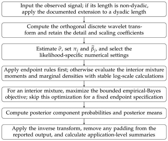
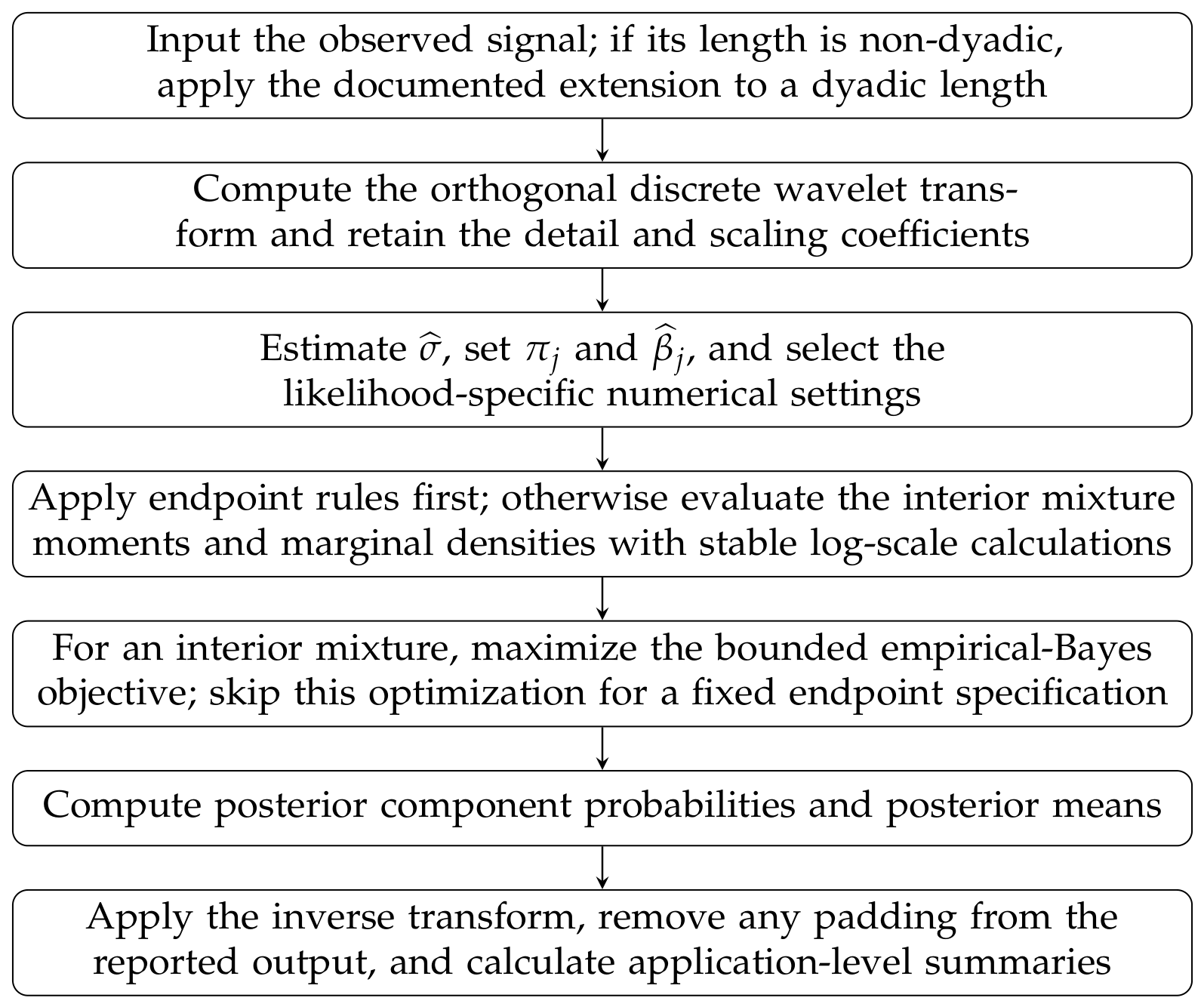
5.3. Fitting Algorithm

The complete fitting procedure is as follows.

Step 1:

Apply an orthogonal DWT to $\mathbf{y}$, obtaining empirical detail coefficients $d_{j,k}$ and scaling coefficients.

Step 2:

Estimate $\widehat{\sigma }$ using (36) and select the Gaussian likelihood $(q=N)$ or the Laplace working likelihood $(q=L)$, with the corresponding quantities defined above.

Step 3:

Set ${\pi }_j$, ${\widehat{\beta }}_j^{\left(0\right)}$, and ${\widehat{\beta }}_j$ using (12), (14), and (15); retain $\varkappa$, ${\epsilon }_{\beta }$, and the selected quadrature order as part of the fitting specification.

Step 4:

Apply the endpoint branches before evaluating unnecessary component expressions. If ${\pi }_j=1$, set the posterior mean and continuous-component probabilities to zero for that level. If ${\pi }_j=0$, omit the spike term. If ${\omega }_j=1$ or ${\omega }_j=0$, evaluate only the Wendland or semicircle component, respectively.

Step 5:

For an interior mixture, evaluate the mixture moments and marginal densities for a candidate $\mathit{\eta }$ as defined in (38) and (39). Use log-sum-exp calculations and the stated numerical safeguards.

Step 6:

If the Gaussian likelihood is selected, maximize (40) to obtain ${\widehat{\mathit{\eta }}}_N$; if the Laplace working likelihood is selected, maximize (41) to obtain ${\widehat{\mathit{\eta }}}_L$. Skip this optimization for a fixed endpoint specification.

Step 7:

Compute the posterior component probabilities and posterior mean for every detail coefficient using the appropriate interior or endpoint map, and save the branch, convergence status, boundary-hit status, warnings, and support diagnostics.

Step 8:

Apply the inverse DWT, retaining the empirical scaling coefficients, to obtain the denoised estimate $\widehat{f}$. For a padded input, retain only the original observations before calculating reported application-level summaries.

The overall fitting workflow is summarized in Figure 3.

Figure 3. Flowchart for the empirical-Bayes wavelet-fitting procedure. Endpoint branches are evaluated before unnecessary component calculations; for a padded record, truncation to the original observations occurs before application-level diagnostics are reported.

6. Simulation Study

The simulation study had two purposes. The primary experiment compared reconstruction accuracy and computational cost over standard test signals, sample sizes, and signal-to-noise ratios. The supplementary experiments then examined the contribution of the two slab components, the resolution-adaptive mixture weight, numerical quadrature, fixed hyperparameters, support saturation, the wavelet basis and coarsest shrunk resolution, non-Gaussian errors, and semi-synthetic seismic recovery (Supplementary Section S3.2). All methods were evaluated on the same simulated realization within each scenario, so that paired comparisons could be formed directly.

6.1. Test Functions and Data Generation

Let f be one of the four standard test functions of Donoho and Johnstone [1]—Bumps, Blocks, Doppler, and HeaviSine. On $[0,1]$, the functions used in the simulations were as follows. Let $sgn\left(u\right)$ denote the sign function. The Blocks function was

$$f_{\mathrm{Blocks}}\left(x\right)={\displaystyle \sum _{r=1}^{11}}{h}_r{\displaystyle \frac{1+sgn(x-t_r)}{2}},$$

where

$$\begin{array}{cc}\hfill (t_1,\dots ,t_{11})=& (0.10,0.13,0.15,0.23,0.25,0.40,0.44,0.65,0.76,0.78,0.81),\hfill \\ \hfill (h_1,\dots ,h_{11})=& (4,-5,3,-4,5,-4.2,2.1,4.3,-3.1,2.1,-4.2).\hfill \end{array}$$

The Bumps function was

$$f_{\mathrm{Bumps}}\left(x\right)={\displaystyle \sum _{r=1}^{11}}{h}_r{\left\{1+\left|{\displaystyle \frac{x-t_r}{w_r}}\right|\right\}}^{-4},$$

where

$$\begin{array}{cc}\hfill (t_1,\dots ,t_{11})=& (0.10,0.13,0.15,0.23,0.25,0.40,0.44,0.65,0.76,0.78,0.81),\hfill \\ \hfill (h_1,\dots ,h_{11})=& (4,5,3,4,5,4.2,2.1,4.3,3.1,5.1,4.2),\hfill \\ \hfill (w_1,\dots ,w_{11})=& (0.005,0.005,0.006,0.010,0.010,0.030,0.010,0.010,0.005,0.008,0.005).\hfill \end{array}$$

The Doppler and HeaviSine functions were

$$\begin{array}{c}{f}_{\mathrm{Doppler}}\left(x\right)=\sqrt{x(1-x)}sin\left\{{\displaystyle \frac{2\pi (1+0.05)}{x+0.05}}\right\},\\ f_{\mathrm{HeaviSine}}\left(x\right)=4sin\left(4\pi x\right)-sgn(x-0.3)-sgn(0.72-x).\end{array}$$

For each function, the observations were generated at $x_i=(i-1)/(n-1)$, with $n\in \{512,1024,2048\}$, according to

$$y_i^{\left(r\right)}=f\left(x_i\right)+{\epsilon }_i^{\left(r\right)},{\epsilon }_i^{\left(r\right)}\stackrel{\mathrm{iid}}{\sim }\mathcal{N}(0,{\sigma }^2),i=1,\dots ,n,$$

where $r=1,\dots ,R$ indexes the $R=100$ independent replications. The primary grid used $\rho \in \{0.2,1,3\}$ for all three sample sizes. To address the sensitivity of conclusions to the very low-SNR setting, the expanded primary grid additionally used $\rho \in \{0.5,2,5\}$ at $n=1024$. For every signal and sample size, the noise scale was set to

$$\sigma ={\displaystyle \frac{SD\{f\left(x_i\right):i=1,\dots ,n\}}{\rho }}.$$

Thus, $\rho$ is an amplitude or standard-deviation SNR, not a power ratio. The corresponding power SNR is ${\rho }^2$, and the decibel representation is $20{log}_{10}\left(\rho \right)$. For example, $\rho =0.2$ corresponds to a power SNR of $0.04$ and $-13.98$ dB, whereas $\rho =5$ corresponds to a power SNR of 25 and $13.98$ dB. The value $0.2$ was retained as a deliberately difficult stress test, while the additional values $0.5$, 2, and 5 provide a wider range of more moderate and favorable conditions. A common random-number construction was used within every scenario: one noise vector was generated for the scenario and passed to all fitted methods.

6.2. Methods and Implementation

The primary method was the adaptive Wendland–semicircle mixture with a Gaussian coefficientwise likelihood, denoted WS–Gaussian or WS–G. The same prior fitted with a Laplace working likelihood, denoted WS–Laplace or WS–L, was included as a robustness and likelihood-sensitivity comparison. The benchmark methods were universal soft thresholding (Univ) [1], false-discovery-rate thresholding (FDR) [5], cross-validation thresholding (CV) [6], Stein’s unbiased risk estimate thresholding (SURE) [2], the Bayesian adaptive multiresolution shrinker (BAMS) [8], and the nonlocal-prior method (NLP) [15]. The comparison was restricted to methods with working software implementations in the analysis environment.

All methods used a Daubechies extremal-phase wavelet with filter number 10, periodic boundary handling, and $J_0=0$, with the alternative basis and $J_0$ checks reported in Supplementary Section S2.6. The proposed fits used $\ell =2$, $\gamma =2.4$, $\varkappa =0.99$, and the quadrature order selected by the independent quadrature study, $q=128$. The BAMS calculation used 32 quadrature points. The finite-sum Wendland calculation was used where available under the Laplace working likelihood, and the specified quadrature order was used for the remaining component calculations. The four classical procedures used soft thresholding. NLP was fitted with the NLPwavelet implementation using its nonlocal-prior mixture, generalized-logit mixture probabilities, double-exponential scale specification, and default values for other settings. The fixed hyperparameters and their perturbations are examined in Supplementary Section S2.5.

6.3. Performance Measures

Let ${\widehat{f}}_i^{\left(r\right)}$ denote the reconstruction in replication r. We recorded the replication-specific mean squared error (MSE), mean absolute error (MAE), maximum absolute error, truth-based output SNR, and elapsed fitting time. In addition to the raw MSE, we used the normalized MSE,

$${NMSE}^{\left(r\right)}={\displaystyle \frac{{MSE}^{\left(r\right)}}{Var\{f\left(x_i\right):i=1,\dots ,n\}}},$$

which permits a more interpretable descriptive comparison across test functions with different scales. The truth-based output SNR was

$${SNR}_{\mathrm{out}}^{\left(r\right)}={\displaystyle \frac{SD\{f\left(x_i\right):i=1,\dots ,n\}}{SD\{{\widehat{f}}_i^{\left(r\right)}-f\left(x_i\right):i=1,\dots ,n\}}}.$$

For a competitor m, the paired MSE and NMSE differences were defined as

$${\Delta }_m^{\mathrm{MSE},\left(r\right)}={MSE}_{\mathrm{WS}-\mathrm{G}}^{\left(r\right)}-{MSE}_m^{\left(r\right)},{\Delta }_m^{\mathrm{NMSE},\left(r\right)}={NMSE}_{\mathrm{WS}-\mathrm{G}}^{\left(r\right)}-{NMSE}_m^{\left(r\right)}.$$

The reporting script summarizes each mean with its Monte Carlo standard error and a replicate-level 95% t-interval. Negative paired differences favor WS–G, whereas a paired win rate is the proportion of common replications for which WS–G has the smaller error. Study-level fit counts and numerical warnings are reported in Supplementary Table S3.

6.4. Primary Gaussian-Error Results

The original 36-cell Gaussian-error grid contains four signals, three sample sizes, and three SNR values. Table 2 reports the complete cellwise MSE comparison; entries in parentheses are Monte Carlo standard errors. The WS–G fit was the best non-NLP method in 24 of the 36 original cells and in 11 of the 12 low-SNR cells (the four signals at each of the three sample sizes). The cellwise results also make explicit how the relative standing of the proposed fits and the benchmark methods changes with signal structure, sample size, and noise level.

Table 2. Mean MSE across 100 independent replications for the original Gaussian-error grid. Each entry is the mean MSE with its Monte Carlo standard error in parentheses; the smallest MSE in each cell is shown in bold.

Signal	SNR	WS–G	WS–L	Univ	FDR	CV	SURE	BAMS	NLP
$n=512$
Bumps	0.2	0.446 (0.005)	0.444 (0.003)	0.450 (0.003)	0.451 (0.003)	0.456 (0.004)	0.554 (0.026)	0.441 (0.003)	0.627 (0.023)
Bumps	1.0	0.227 (0.003)	0.357 (0.002)	0.370 (0.002)	0.319 (0.003)	0.180 (0.002)	0.187 (0.003)	0.382 (0.002)	0.133 (0.001)
Bumps	3.0	0.049 (0.001)	0.148 (0.002)	0.179 (0.001)	0.091 (0.001)	0.051 (0.000)	0.038 (0.001)	0.234 (0.002)	0.026 (0.000)
Blocks	0.2	3.305 (0.053)	3.610 (0.030)	3.770 (0.027)	3.822 (0.024)	3.716 (0.042)	4.445 (0.146)	3.558 (0.028)	3.946 (0.213)
Blocks	1.0	0.898 (0.012)	1.439 (0.010)	1.667 (0.014)	1.554 (0.018)	0.871 (0.009)	0.933 (0.013)	1.514 (0.010)	0.582 (0.007)
Blocks	3.0	0.307 (0.003)	0.524 (0.005)	0.715 (0.005)	0.481 (0.006)	0.217 (0.002)	0.241 (0.004)	0.706 (0.008)	0.172 (0.002)
Doppler	0.2	0.077 (0.001)	0.081 (0.001)	0.087 (0.001)	0.087 (0.001)	0.087 (0.001)	0.108 (0.004)	0.081 (0.001)	0.088 (0.004)
Doppler	1.0	0.015 (0.000)	0.031 (0.001)	0.038 (0.000)	0.033 (0.001)	0.017 (0.000)	0.018 (0.000)	0.050 (0.001)	0.011 (0.000)
Doppler	3.0	0.003 (0.000)	0.008 (0.000)	0.011 (0.000)	0.007 (0.000)	0.003 (0.000)	0.003 (0.000)	0.017 (0.000)	0.002 (0.000)
HeaviSine	0.2	4.798 (0.256)	7.060 (0.161)	8.072 (0.162)	9.080 (0.093)	7.095 (0.231)	10.096 (0.829)	7.784 (0.116)	5.310 (0.314)
HeaviSine	1.0	0.475 (0.017)	0.904 (0.013)	1.403 (0.023)	1.746 (0.074)	0.791 (0.018)	0.851 (0.022)	0.927 (0.018)	0.323 (0.017)
HeaviSine	3.0	0.111 (0.002)	0.158 (0.002)	0.319 (0.004)	0.362 (0.015)	0.153 (0.002)	0.163 (0.003)	0.312 (0.005)	0.075 (0.002)
$n=1024$
Bumps	0.2	0.431 (0.003)	0.447 (0.001)	0.456 (0.001)	0.456 (0.001)	0.453 (0.002)	0.485 (0.007)	0.444 (0.001)	0.460 (0.010)
Bumps	1.0	0.151 (0.001)	0.301 (0.002)	0.313 (0.002)	0.248 (0.002)	0.130 (0.001)	0.140 (0.001)	0.350 (0.001)	0.092 (0.001)
Bumps	3.0	0.029 (0.000)	0.083 (0.001)	0.108 (0.001)	0.058 (0.001)	0.025 (0.000)	0.025 (0.000)	0.172 (0.002)	0.017 (0.000)
Blocks	0.2	2.604 (0.053)	3.334 (0.028)	3.574 (0.027)	3.707 (0.018)	3.311 (0.048)	3.769 (0.116)	3.354 (0.024)	2.497 (0.111)
Blocks	1.0	0.619 (0.006)	1.147 (0.010)	1.253 (0.010)	1.147 (0.014)	0.673 (0.005)	0.701 (0.006)	1.331 (0.007)	0.420 (0.004)
Blocks	3.0	0.209 (0.002)	0.409 (0.002)	0.516 (0.003)	0.351 (0.003)	0.159 (0.001)	0.172 (0.002)	0.520 (0.003)	0.122 (0.001)
Doppler	0.2	0.068 (0.001)	0.078 (0.000)	0.084 (0.000)	0.085 (0.000)	0.081 (0.001)	0.089 (0.002)	0.079 (0.000)	0.054 (0.002)
Doppler	1.0	0.010 (0.000)	0.020 (0.000)	0.027 (0.000)	0.024 (0.000)	0.012 (0.000)	0.013 (0.000)	0.032 (0.000)	0.007 (0.000)
Doppler	3.0	0.002 (0.000)	0.004 (0.000)	0.006 (0.000)	0.005 (0.000)	0.002 (0.000)	0.002 (0.000)	0.013 (0.000)	0.001 (0.000)
HeaviSine	0.2	2.619 (0.090)	4.915 (0.141)	6.072 (0.142)	8.447 (0.122)	4.840 (0.141)	5.788 (0.246)	6.422 (0.151)	2.993 (0.233)
HeaviSine	1.0	0.253 (0.007)	0.603 (0.015)	0.961 (0.016)	1.120 (0.028)	0.519 (0.010)	0.553 (0.012)	0.707 (0.015)	0.204 (0.008)
HeaviSine	3.0	0.080 (0.001)	0.118 (0.001)	0.211 (0.003)	0.230 (0.016)	0.109 (0.001)	0.114 (0.002)	0.281 (0.004)	0.052 (0.001)
$n=2048$
Bumps	0.2	0.406 (0.002)	0.434 (0.001)	0.446 (0.001)	0.448 (0.001)	0.441 (0.002)	0.466 (0.006)	0.434 (0.001)	0.346 (0.007)
Bumps	1.0	0.092 (0.001)	0.207 (0.002)	0.225 (0.001)	0.174 (0.001)	0.092 (0.001)	0.096 (0.001)	0.288 (0.001)	0.058 (0.001)
Bumps	3.0	0.017 (0.000)	0.050 (0.000)	0.065 (0.000)	0.037 (0.000)	0.016 (0.000)	0.017 (0.000)	0.107 (0.000)	0.010 (0.000)
Blocks	0.2	1.904 (0.034)	2.967 (0.030)	3.246 (0.032)	3.487 (0.027)	2.720 (0.045)	2.898 (0.057)	3.090 (0.027)	1.739 (0.050)
Blocks	1.0	0.472 (0.003)	0.789 (0.007)	0.960 (0.006)	0.850 (0.007)	0.520 (0.004)	0.535 (0.004)	1.020 (0.009)	0.298 (0.003)
Blocks	3.0	0.129 (0.001)	0.305 (0.001)	0.364 (0.002)	0.246 (0.002)	0.114 (0.001)	0.120 (0.001)	0.413 (0.002)	0.077 (0.001)
Doppler	0.2	0.052 (0.001)	0.072 (0.000)	0.081 (0.000)	0.083 (0.000)	0.071 (0.001)	0.074 (0.001)	0.077 (0.000)	0.033 (0.001)
Doppler	1.0	0.006 (0.000)	0.013 (0.000)	0.018 (0.000)	0.016 (0.000)	0.008 (0.000)	0.008 (0.000)	0.023 (0.000)	0.004 (0.000)
Doppler	3.0	0.001 (0.000)	0.003 (0.000)	0.004 (0.000)	0.003 (0.000)	0.001 (0.000)	0.001 (0.000)	0.011 (0.000)	0.001 (0.000)
HeaviSine	0.2	1.654 (0.053)	2.891 (0.092)	4.499 (0.093)	6.986 (0.188)	3.313 (0.085)	3.780 (0.111)	4.812 (0.177)	1.516 (0.104)
HeaviSine	1.0	0.158 (0.003)	0.273 (0.005)	0.609 (0.008)	0.717 (0.019)	0.342 (0.005)	0.366 (0.007)	0.469 (0.009)	0.138 (0.005)
HeaviSine	3.0	0.051 (0.001)	0.094 (0.001)	0.145 (0.001)	0.136 (0.002)	0.075 (0.001)	0.078 (0.001)	0.287 (0.003)	0.034 (0.000)

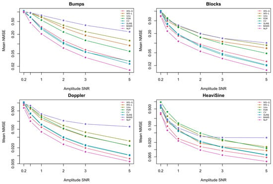
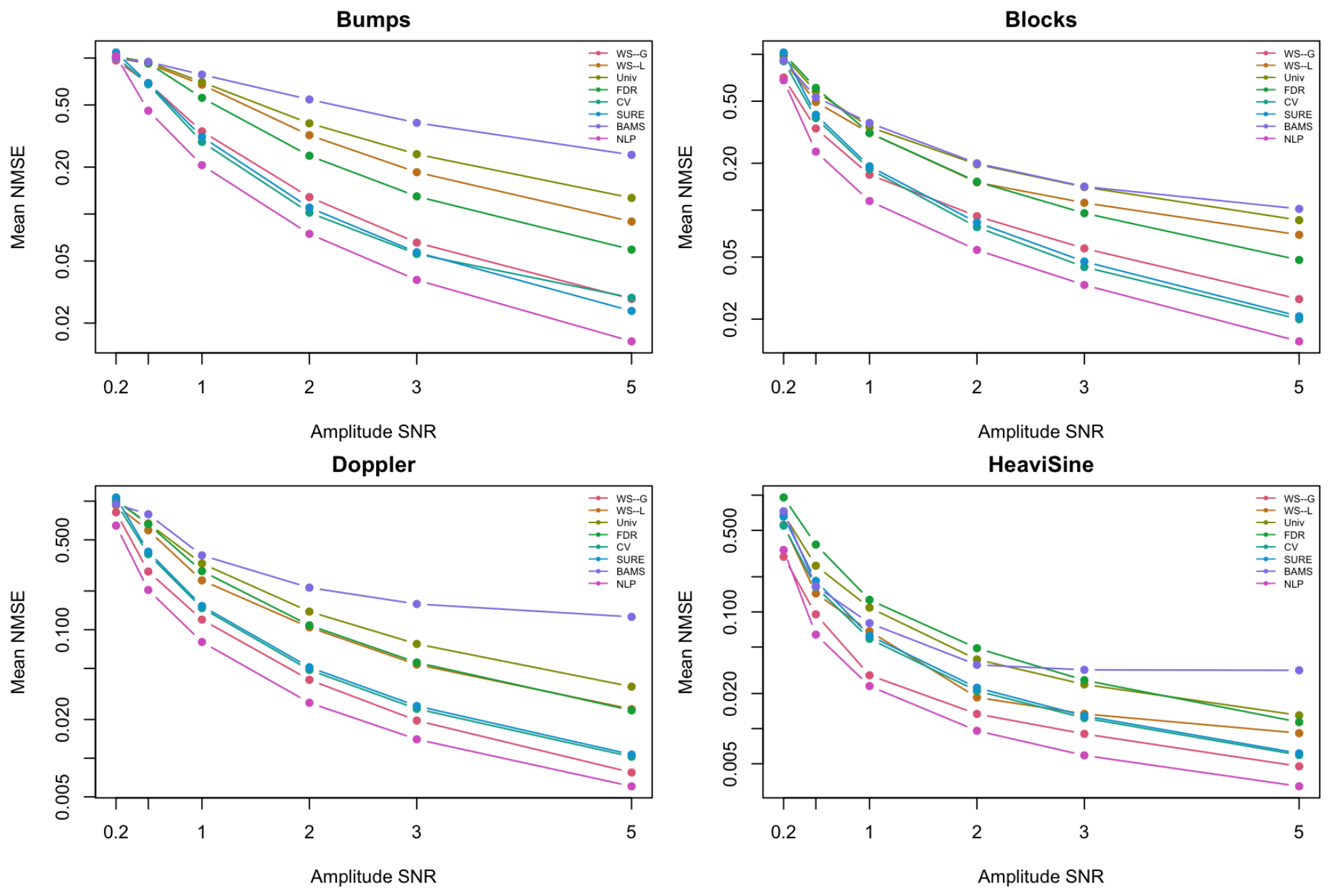
Figure 4 displays normalized-error profiles over the expanded SNR range at $n=1024$. The additional SNR values test whether the low-SNR ranking persists away from $\rho =0.2$, while the normalization prevents the large-scale Blocks and HeaviSine signals from dominating the visual comparison. The figure is descriptive; the detailed cellwise MSE values remain the primary accuracy comparison.

Figure 4. Mean NMSE as a function of amplitude SNR at $n=1024$ over the expanded primary Gaussian-error grid. Panels correspond to Bumps, Blocks, Doppler, and HeaviSine; each point averages 100 common-random-number replications, and lower values indicate better reconstruction accuracy.

Table 3 summarizes the primary Gaussian-error simulations based on the four deterministic Donoho–Johnstone test functions, averaged over the 36 signal–sample-size–SNR cells with 100 common-random-number replications per cell; MSE and NMSE are computed against the known generating functions. Because the test functions have different scales, these pooled averages should not be interpreted as a universal method ranking; normalized and cellwise summaries are more informative. NLP attains the smallest pooled mean MSE and NMSE, whereas WS–G is the best non-NLP method in 24 of the 36 cells. WS–G has mean MSE 0.631 and mean NMSE 0.306, compared with mean MSE 0.624 and mean NMSE 0.287 for NLP. This accuracy advantage for NLP comes at a substantial computational cost: its mean fitting time is $116.442\mathrm{s}$ per replicate, compared with $0.281\mathrm{s}$ for WS–G. Thus, the table indicates an accuracy–computational-cost trade-off rather than a universal pooled-MSE ordering.

Table 3. Descriptive averages over the original 36 Gaussian-error design cells. NMSE is normalized by the variance of the corresponding true signal; runtime is the mean elapsed time in seconds per fitted replicate; best values for each numerical measure are shown in bold.

Method	Mean MSE	Mean NMSE	Mean MAE	Mean Output SNR	Runtime (s)	Best Non-NLP Cells
WS–G	0.631	0.306	0.435	3.807	0.281	24
WS–L	0.953	0.423	0.557	2.714	1.816	0
Univ	1.148	0.476	0.631	2.268	0.003	0
FDR	1.308	0.468	0.649	2.433	0.003	0
CV	0.879	0.358	0.511	3.381	0.011	10
SURE	1.054	0.406	0.529	3.302	0.003	1
BAMS	1.132	0.495	0.626	2.077	0.012	1
NLP	0.624	0.287	0.408	4.593	116.442	–

6.4.1. What Is Gained by the Adaptive Mixture?

The central ablation compares four Gaussian WS specifications: Wendland-only (${\omega }_j=1$), Semicircle-only (${\omega }_j=0$), a constant mixture with only the intercept estimated, and the proposed adaptive mixture with both the intercept and resolution trend estimated. The comparison uses the component/adaptivity study over all three sample sizes, all three original SNR values, and all four signals. Table 4 reports normalized and raw error summaries together with cellwise wins and paired differences. The adaptive fit was the lowest-NMSE specification in 8 of the 36 ablation cells, whereas the Semicircle-only endpoint was lowest in 26 cells. Its paired win rate against the constant mixture was 72.6%. Thus, the ablation does not indicate a uniform accuracy gain from resolution-dependent mixing; rather, it shows that the adaptive mixture is a flexible specification whose benefit depends on the signal and noise level.

Table 4. Gaussian WS component and adaptivity ablation over the 36 original signal–sample-size–SNR cells. Best MSE/NMSE values are bolded. The paired difference is adaptive WS–G minus the indicated specification; negative values favor the adaptive mixture.

Specification	Mean NMSE	Mean MSE	Lowest-NMSE Cells	Paired NMSE Difference [95% CI]	Adaptive Win Rate (%)
WS–G	0.306	0.631	8	–	–
WS–G constant	0.306	0.632	1	−0.000224 [−0.000344, −0.000104]	72.6
Wendland-only	0.349	0.766	1	−0.042523 [−0.044524, −0.040521]	97.1
Semicircle-only	0.306	0.631	26	0.000284 [0.000205, 0.000363]	25.7

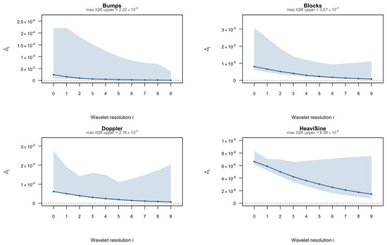
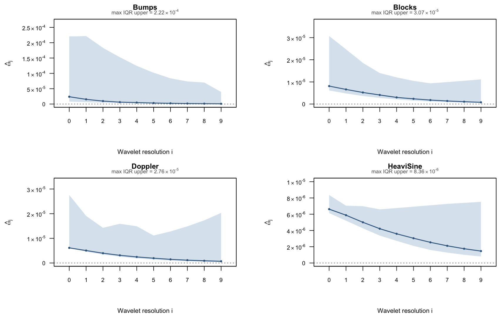
Figure 5 shows the fitted adaptive Wendland weight profiles at $n=1024$ and $\rho =0.2$. The solid curve is the replicate median and the shaded region is the interquartile range. Although the weights are positive, they are extremely close to zero in this slice: all median weights are below $2.4\times {10}^{-5}$, and all upper-quartile values are below $2.3\times {10}^{-4}$. Thus, the adaptive fit is close to the Semicircle-only endpoint ${\omega }_j=0$; the figure should be interpreted as showing weak data-driven variation around that endpoint, not substantial resolution-varying use of both components.

Figure 5. Fitted Wendland mixture-weight profiles ${\widehat{\omega }}_j$ for the adaptive WS–Gaussian fit at $n=1024$ and amplitude SNR $\rho =0.2$. Panels correspond to the four test signals. Curves show replicate medians and ribbons show interquartile ranges. Signal-specific zoomed vertical axes display the small positive weights; the dotted horizontal line marks the Semicircle-only endpoint ${\omega }_j=0$, while the Wendland-only endpoint ${\omega }_j=1$ lies outside the plotted ranges.

6.4.2. Paired and Normalized Comparisons

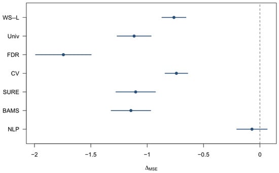
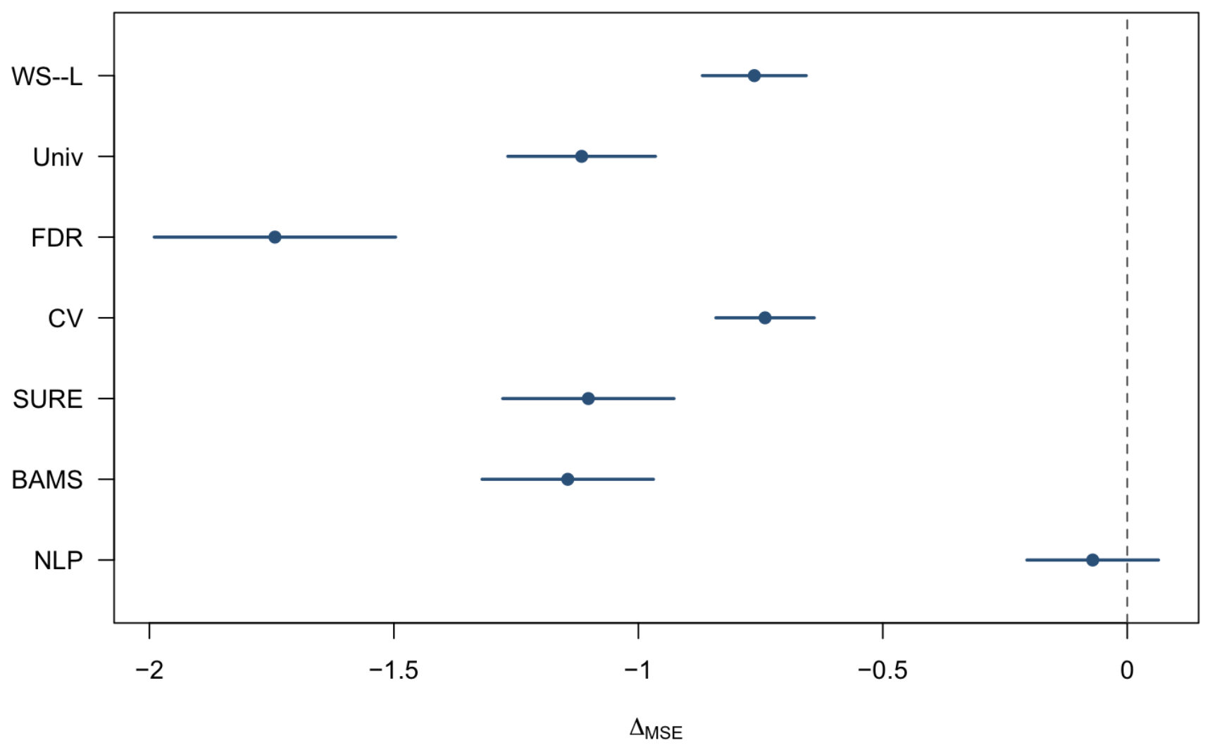
At $n=1024$ and $\rho =0.2$, Table 5 reports paired MSE and NMSE differences pooled over the four signals and 100 common replications per signal. The interval for each difference uses the empirical standard deviation of the paired replicate differences, rather than separate intervals for the two method means. The 95% intervals for the WS–G versus NLP comparison include zero for both MSE and NMSE, and the WS–G win rate is 38.5%; therefore, this low-SNR slice does not establish an advantage for WS–G over NLP. The negative differences and win rates for the other comparisons indicate where WS–G has a reproducible low-SNR advantage and where competing methods remain competitive. Figure 6 gives the corresponding MSE-difference intervals on a common scale.

Table 5. Paired comparison with WS–Gaussian at (n = 1024) and amplitude SNR (0.2), pooled over the four signals and 100 common-random-number replications per signal. Negative differences favor WS–Gaussian.

Competitor	MSE Difference [95% CI]	NMSE Difference [95% CI]	WS–G Win Rate (%)
WS–L	−0.763 [−0.869, −0.657]	−0.151 [−0.163, −0.139]	94.2
Univ	−1.116 [−1.267, −0.965]	−0.225 [−0.241, −0.209]	98.0
FDR	−1.743 [−1.990, −1.496]	−0.305 [−0.329, −0.280]	98.8
CV	−0.741 [−0.841, −0.640]	−0.162 [−0.172, −0.151]	97.5
SURE	−1.102 [−1.277, −0.927]	−0.262 [−0.287, −0.237]	98.2
BAMS	−1.144 [−1.320, −0.969]	−0.198 [−0.217, −0.180]	93.2
NLP	−0.071 [−0.205, 0.064]	0.024 [−0.006, 0.053]	38.5

Figure 6. Paired mean MSE differences at $n=1024$ and amplitude SNR $\rho =0.2$, pooled over the four test signals. Points are mean differences ${MSE}_{\mathrm{WS}-\mathrm{G}}-{MSE}_m$, and horizontal intervals are replicate-level 95% t-intervals. Negative values favor WS–Gaussian.

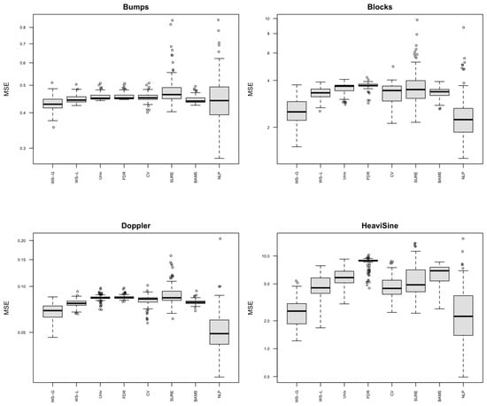
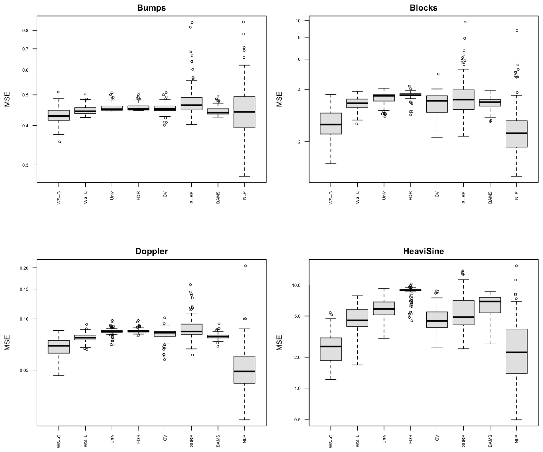
Figure 7 shows the replicate-level MSE distributions and the spread and outliers underlying the paired summaries in Table 5.

Figure 7. Replicate-specific Box plots, showing MSE distributions at $n=1024$ and amplitude SNR $\rho =0.2$, shown separately for the four test signals. Each box summarizes the 100 common-random-number replications for each method.

6.5. Interpretation

The primary simulation supports a qualified conclusion. At the representative low-SNR slice, the pooled MSE leader is WS–G, while the full cellwise table shows which signals and resolutions drive that summary. WS–G is the best non-NLP method in 24 of the original cells, and its performance should therefore be interpreted as a cellwise advantage in the difficult settings where it occurs rather than as uniform dominance. The ablation and fitted-weight results show that the model provides two alternative compact-support slab shapes and permits resolution-dependent weighting, but the fitted weights in the examined low-SNR slice were close to the Semicircle-only endpoint; thus, the present results do not demonstrate a substantial accuracy gain from resolution-dependent mixing.

The supplementary analyses quantify how sensitive this interpretation is to numerical and tuning choices. The quadrature study selects the smallest order whose reconstruction, component-moment, and MSE changes remain below prespecified tolerances. The hyperparameter and support analyses assess the fixed sparsity schedule, empirical support quantile, and possible saturation of large coefficients. The Laplace-error experiment evaluates a different data-generating mechanism and therefore is a sensitivity analysis rather than an estimate of the Gaussian-error risk. Finally, the semi-synthetic seismic experiment uses a processed trace as a known surrogate truth after adding controlled noise; it complements, but does not replace, the real-data illustration for which no noise-free reference waveform is available.

7. Seismic-Trace Data Application

The simulation study evaluates denoising accuracy against a known signal. For a measured seismic record, however, a noise-free reference acceleration is not available. We therefore use the real-data analysis as an illustration of the reconstructed waveform and compare the methods using signal-level diagnostics—residual variability, sample-to-sample residual roughness, retained squared-energy, preservation and timing of the largest absolute acceleration, and visual agreement with the observed trace. These quantities describe how aggressively each method modifies the record. They should not be interpreted as out-of-sample accuracy measures in the absence of a trusted reference signal.

7.1. Record and Data Extraction

The record was obtained through the United States Geological Survey (USGS) Earthquake Data portal https://www.usgs.gov/programs/earthquake-hazards/science/earthquake-data, which directs processed strong-motion waveform downloads to the Center for Engineering Strong Motion Data (CESMD) https://www.strongmotioncenter.org/ (both data links accessed on 10 August 2026). USGS Specifically, we downloaded the 29 July 2008 Chino Hills earthquake record from station 24763, which corresponds to Sylmar–Olive View Hospital Grounds. The station coordinates are $34.{327}^{\circ }\mathrm{N}$ and $118.{444}^{\circ }\mathrm{W}$, and the record identifier is 24763-K0186-08211.01.

The time-domain data were extracted from CE24763.V2, which contains the corrected accelerogram blocks. The companion file CE24763.V3 contains the response and Fourier-amplitude spectra and was not used as the time-domain input. In the main text, we analyze channel 1, the horizontal component labeled ${360}^{\circ }$. The results for channels 2 and 3, labeled Up and ${90}^{\circ }$, respectively, are provided in the Supplementary Materials.

The source file reports instrument- and baseline-corrected acceleration and a bandpass with 3 dB points at $0.30$ and $40.00$ Hz. We used the acceleration block supplied in that file without applying an additional filter, detrending operation, or unit conversion. We used a fixed-width parser that read eight values per line using 10-character fields and retained the first $N=\mathrm{15,400}$ acceleration values. Let $a_i$ denote the ith observed acceleration, measured in $\mathrm{cm}{\mathrm{s}}^{-2}$, and let $\Delta t=0.005$ s denote the sampling interval. The corresponding sampling frequency is $f_s=1/\Delta t=200$ Hz, and the observation times are $t_i=(i-1)\Delta t$, $i=1,\dots ,N$. Thus, the record spans 0 to $76.995$ s, with a nominal duration of $77.000$ s. The observed acceleration ranges from $-44.27435$ to $36.89636$$\mathrm{cm}{\mathrm{s}}^{-2}$; the largest observed absolute acceleration is $44.27435\mathrm{cm}{\mathrm{s}}^{-2}$ at approximately $36.05$ s. The data and common analysis settings are summarized in Table 6.

Table 6. Data and common analysis settings for the seismic application.

Quantity	Specification
Earthquake and date	Chino Hills earthquake, 29 July 2008
Station and record	Station 24763; record 24763-K0186-08211.01
Input file and component	CE24763.V2, channel 1, ${360}^{\circ }$ horizontal component
Original observations	$N=\mathrm{15,400}$ acceleration values
Sampling interval and frequency	$\Delta t=0.005$ s and $f_s=200$ Hz
Units and duration	$\mathrm{cm}{\mathrm{s}}^{-2}$; 77.000 s nominal duration
Source processing	Instrument- and baseline-corrected; 0.30–40.00 Hz bandpass reported by CESMD
Wavelet input length	$2^{14}=\mathrm{16,384}$, obtained by appending 984 reverse-padded values
Wavelet basis	Daubechies extremal-phase family, DaubExPhase, filter number 10
Boundary rule and coarsest level	Periodic boundary rule; $J_0=0$
WS tuning settings	$\beta$-quantile $=0.99$, spike offset $=2$, spike exponent $\gamma =2.4$, quadrature order $=48$
Fitted methods	WS–Gaussian, WS–Laplace, Wendland-only, Semicircle-only, Univ, FDR, CV, and SURE

7.2. Padding and Wavelet Analysis

Because the original record has length $N=\mathrm{15,400}$, which is not a power of two, the wavelet input was extended to $\tilde{N}=\mathrm{16,384}=2^{14}$ observations. Thus, $J={log}_2\left(\tilde{N}\right)=14$, and the detail levels in the padded analysis are $j=J_0,\dots ,13$. Specifically, 984 values were appended in reverse order from the end of the observed record. This reverse-padding rule avoids discarding observations and reduces the artificial endpoint jump that would result from simply appending zeros. The periodic boundary rule was then applied to the padded signal. After reconstruction, only the first N fitted values were retained, so all reported diagnostics refer to the original 77-s record.

All methods used the Daubechies extremal phase wavelet family with filter number 10, periodic boundary handling, and $J_0=0$. The proposed Wendland–semicircle model was fitted with a Gaussian likelihood (WS–Gaussian) and a Laplace likelihood (WS–Laplace). For the two component-specific fits, Wendland-only fixes the resolution-specific Wendland mixture weight at ${\omega }_j=1$, whereas Semicircle-only fixes it at ${\omega }_j=0$, where ${\omega }_j$ denotes the mixture weight assigned to the Wendland component at wavelet resolution j. The support-scale quantile, spike prior offset, spike exponent, and quadrature settings were $0.99$, 2, $2.4$, and 48, respectively, as summarized in Table 6. For comparison, Univ, FDR, CV, and SURE were used. These four classical rules used the same wavelet basis and boundary rule as the proposed method.

7.3. Real-Data Diagnostics

Let ${\widehat{a}}_{m,i}$ denote the reconstructed acceleration at time $t_i$ under method m, and define the residual $e_{m,i}=a_i-{\widehat{a}}_{m,i}$. The residual standard deviation is $SD\left(e_m\right)$, and the sample-to-sample residual roughness is $SD(\Delta e_m)$, where $\Delta e_{m,i}=e_{m,i+1}-e_{m,i}$ for $i=1,\dots ,N-1$. The retained squared-energy ratio is

$$R_m={\displaystyle \frac{{\sum }_{i=1}^N{\widehat{a}}_{m,i}^2}{{\sum }_{i=1}^N{a}_i^2}}.$$

Finally, let $A_m={max}_i\left|{\widehat{a}}_{m,i}\right|$ denote the reconstructed peak absolute acceleration and let $T_m=t_{{\widehat{i}}_m}$, where ${\widehat{i}}_m=arg{max}_i\left|{\widehat{a}}_{m,i}\right|$, denote its time.

Table 7 reports the resulting diagnostics. The WS–Gaussian reconstruction has residual standard deviation $1.2357$ in the input units. Its retained squared-energy ratio is $0.7496$, and its reconstructed peak is $37.4867\mathrm{cm}{\mathrm{s}}^{-2}$ at $36.04$ s. WS–Laplace is nearly identical, while the Wendland-only fit has slightly larger residual variability and residual roughness. The Semicircle-only reconstruction is numerically almost indistinguishable from WS–Gaussian for this record.

Table 7. Signal-level diagnostics for the Chino Hills channel-1 accelerogram. Residual SD and residual roughness are in $\mathrm{cm}{\mathrm{s}}^{-2}$; retained energy is dimensionless; peak acceleration is in $\mathrm{cm}{\mathrm{s}}^{-2}$; and peak time is in seconds. The estimated noise scale is repeated because it was common to all fitted methods.

Method	$\widehat{\mathit{\sigma }}$	Residual SD	Residual Roughness	Retained Energy	Peak $\left|\mathit{a}\right|$	Peak Time
WS–Gaussian	0.001038	1.235737	0.126581	0.749592	37.486663	36.040
WS–Laplace	0.001038	1.235750	0.126616	0.749502	37.489605	36.040
Wendland-only	0.001038	1.259843	0.129444	0.750354	37.419648	36.040
Semicircle-only	0.001038	1.235738	0.126580	0.749643	37.486663	36.040
Univ	0.001038	0.011819	0.008193	0.998916	44.250075	36.050
FDR	0.001038	0.001816	0.001837	0.999871	44.269623	36.050
CV	0.001038	0.012125	0.008371	0.998883	44.249556	36.050
SURE	0.001038	0.001704	0.001747	0.999880	44.269943	36.050

The thresholding reconstructions have residual standard deviations ranging from $0.0017$ to $0.0121$ in the input units. Their sample-to-sample roughness ranges from $0.0017$ to $0.0084$, and their retained-energy ratios exceed $0.9988$. Thus, they remain extremely close to the observed record under these diagnostics and preserve the observed peak of approximately $44.27\mathrm{cm}{\mathrm{s}}^{-2}$ at $36.05$ s. In contrast, the WS fits remove more high-frequency variation and attenuate the absolute peak to approximately $37.42$–$37.49$$\mathrm{cm}{\mathrm{s}}^{-2}$, while preserving its timing to within 0.01 s. Since no clean signal is available, the larger residual and lower retained energy for WS should be interpreted as stronger shrinkage, not automatically as either improvement or deterioration. Supplementary Tables S13 and S14 include similar results for channels 2 and 3, respectively.

7.4. Waveform Comparison

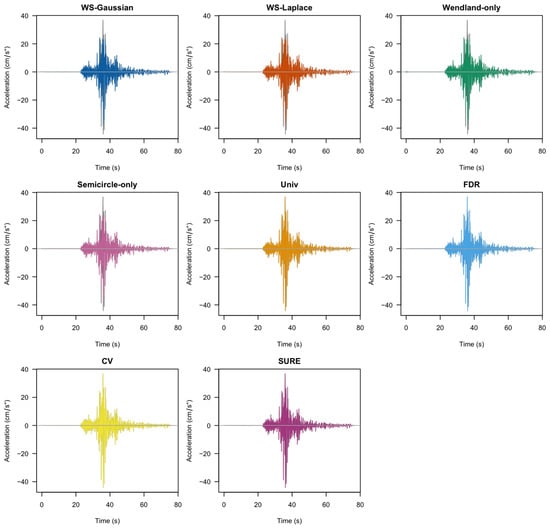
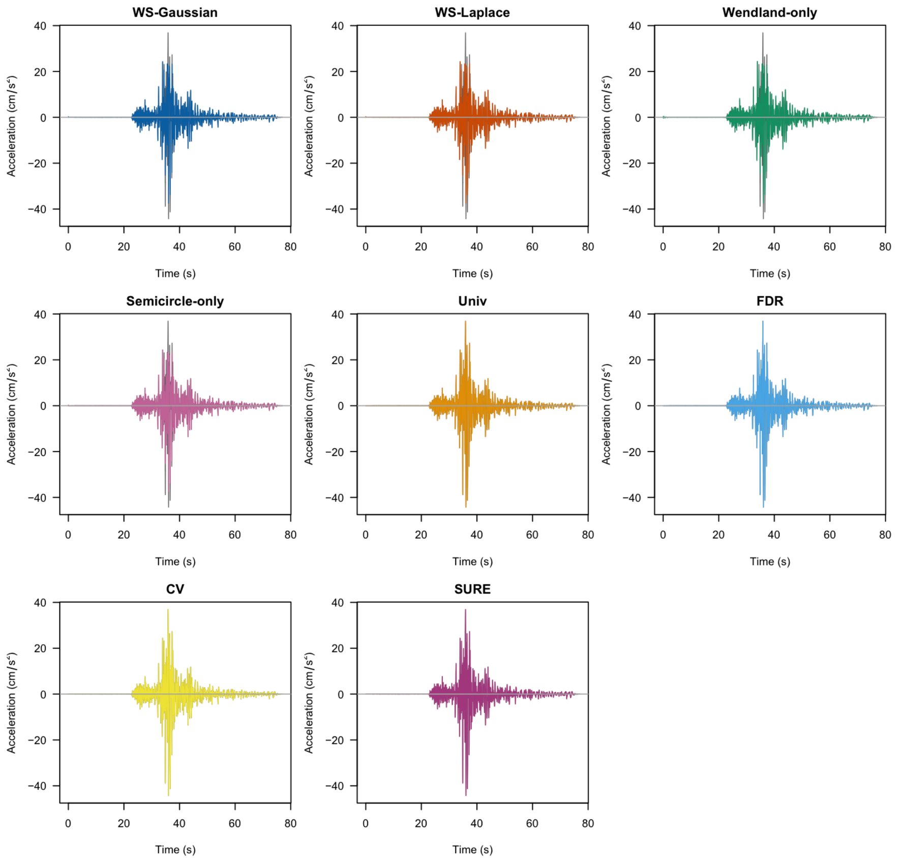
The full-record comparison is shown in Figure 8. The observed acceleration is drawn in gray in every panel, while the colored curve is the reconstruction from the method named in that panel. All methods retain the principal wave packet, its approximate arrival time, and the subsequent decaying oscillations. The WS reconstructions visibly suppress some of the rapid oscillations and reduce the height of the largest extrema, whereas Univ, FDR, CV, and SURE remain nearly superimposed on the observed trace over most of the record. Supplementary Figures S9 and S10 present similar plots for channels 2 and 3, respectively.

Figure 8. Full-record comparison for the 77-s Chino Hills channel-1 accelerogram. In each panel, the gray curve is the observed acceleration and the colored curve is the reconstruction from the indicated method.

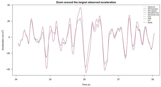
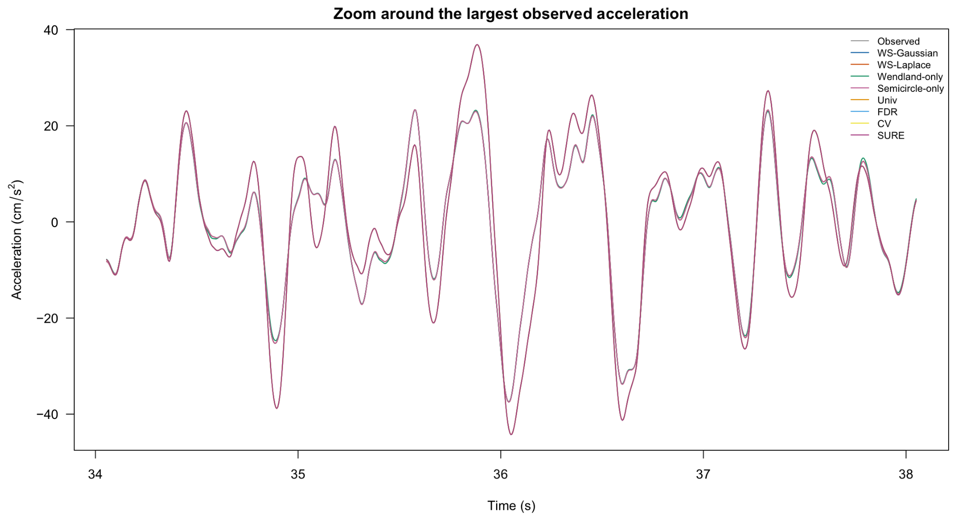
Figure 9 provides a closer view of the interval 34–38 s containing the largest observed absolute acceleration. The WS–Gaussian, WS–Laplace, Wendland-only, and Semicircle-only curves preserve the broad waveform while reducing the most extreme excursions. The thresholding curves preserve the peak more nearly exactly, consistent with the retained-energy and peak diagnostics in Table 7. The near overlap of WS–Gaussian and Semicircle-only in this window is also consistent with their nearly identical signal-level diagnostics.

Figure 9. Zoomed comparison over 34–38 s around the largest observed absolute acceleration. The observed trace and eight reconstructions are shown in $\mathrm{cm}{\mathrm{s}}^{-2}$.

7.5. Interpretation and Limitations

This application demonstrates the operational behavior of the proposed shrinkage model on a processed strong-motion record. WS–Gaussian and WS–Laplace produce almost identical reconstructions for this example, and their output is much closer to the Semicircle-only fit than to the Wendland-only fit. The proposed fits also provide visibly stronger attenuation of rapid fluctuations than the four classical thresholding rules, while preserving the timing of the dominant acceleration pulse. These observations are useful for illustrating the model, but they do not establish that one method has lower denoising risk for real seismic data.

Several limitations should be made explicit. First, the record is a single horizontal component from one earthquake and one station; the results cannot be generalized to other magnitudes, distances, site conditions, components, or recording instruments. Second, the CESMD waveform has already undergone instrument and baseline correction and source-reported bandpass filtering, so the analysis assesses shrinkage conditional on that preprocessing. Third, the periodic boundary rule and reverse-padding construction can affect the two endpoints, although the dominant acceleration pulse is well inside the record. Fourth, the absence of a clean reference prevents direct calculation of MSE, MAE, or true signal-to-noise improvement.

8. Conclusions

We proposed a Bayesian wavelet-shrinkage rule based on a spike at zero and an adaptive mixture of a compactly supported Wendland density and the semicircle density. The Wendland component concentrates more strongly near zero and vanishes smoothly at the support boundary, whereas the semicircle component is more dispersed and can preserve moderate wavelet coefficients. The resulting posterior-mean estimator is computable through two component-specific integrals, with explicit support control through ${\beta }_j$ and adaptive shape selection through the resolution-specific mixture weight ${\omega }_j$.

The simulation results indicate that the proposed WS–Gaussian method is competitive in low-SNR settings. Its pooled mean MSE was $0.631$, compared with $0.624$ for NLP and $0.879$ for CV, and it was the best-performing non-NLP method in 24 of the 36 design cells, including 11 of the 12 low-SNR cells. At $n=1024$ and $\rho =0.2$, WS–Gaussian had lower MSE than each non-NLP competitor in at least $93.2\%$ of paired replications. NLP achieved the best overall reconstruction accuracy, particularly for Doppler and at moderate or favorable SNR, but WS–Gaussian provided a more favorable accuracy–runtime balance than both NLP and the Laplace-working-likelihood version. Thus, the results do not support universal dominance of a single kernel. Instead, they suggest that the usefulness of the Wendland–semicircle construction depends on SNR, signal structure, and computational constraints.

The seismic application provides a complementary illustration without a noise-free reference. WS–Gaussian and WS–Laplace produced nearly identical reconstructions, and the WS–Gaussian output was numerically close to the Semicircle-only reconstruction. Relative to the observed peak acceleration of approximately $44.27\mathrm{cm}{\mathrm{s}}^{-2}$, the proposed fits reduced the peak to approximately $37.49\mathrm{cm}{\mathrm{s}}^{-2}$ while preserving its timing to within $0.01$ s. The classical thresholding methods retained more than $99.8\%$ of the observed squared energy and preserved the observed peak almost exactly. These results illustrate the different shrinkage strengths of the methods, but, because the seismic record does not provide a trusted clean signal, they cannot establish which reconstruction has lower real-data risk.

The semi-synthetic seismic validation complements this real-data illustration by treating the processed channel-1 trace as a surrogate truth and adding independent Gaussian noise at amplitude SNRs $0.5$, 1, 2, and 5. The noisy-observation baseline had mean NMSEs of approximately $3.995$, $0.999$, $0.249$, and $0.040$, respectively, closely matching the expected $1/{\mathrm{SNR}}^2$ pattern. WS–Gaussian improved on this baseline at SNRs $0.5$, 1, and 2, but not at SNR 5, where weak noise made denoising less beneficial. The adaptive WS–Gaussian fit was nearly identical to the Semicircle-only fit, while WS–Laplace exhibited a substantial peak-timing error at SNR 2 (mean $0.412$ s; 72% of replicates exceeded $0.1$ s). These results support the operational use of the method under controlled surrogate-truth conditions, but they do not establish uniform superiority or real-data denoising risk.

The method is formulated for a one-dimensional signal observed on an equally spaced grid and analyzed with an orthogonal discrete wavelet transform. The primary formulation assumes independent errors with a common variance, whereas the Laplace version is a coefficient-wise working likelihood used for sensitivity analysis; it does not assert that a time-domain Laplace error remains exactly Laplace and independent after the discrete wavelet transform. For a non-dyadic record, a deterministic extension to a dyadic length is used, and the reconstructed values are truncated to the original observations before application-level diagnostics are calculated. Conditional on the empirical-Bayes hyperparameters, detail coefficients are modeled independently with symmetric spike-and-slab priors at each resolution, while scaling coefficients are retained rather than shrunk. Consequently, the coefficient-wise construction does not model dependence among neighboring or parent–child coefficients or across resolutions.

The level-specific support interval $[-{\beta }_j,{\beta }_j]$ is an explicit modeling and truncation choice. When ${\beta }_j$ is obtained from an empirical quantile, it is not a formal estimator or guarantee of the true support; coefficients outside the interval are necessarily subject to boundary saturation. The method may therefore be less suitable when errors are strongly correlated or heteroscedastic, when the signal contains frequent large coefficients outside the fitted support, or when the selected wavelet basis and boundary rule inadequately represent the signal. The results are consequently basis-, boundary-, hyperparameter-, and support-rule-dependent, and the present formulation does not directly cover two-dimensional images.

The present method estimates the shape trend through a low-dimensional empirical-Bayes parameterization. A fully Bayesian extension could place a prior on $\mathit{\eta }$, propagate its uncertainty into the posterior mean, and provide posterior uncertainty intervals for ${\omega }_j$ across resolutions. The resolution trend permits, but does not guarantee, meaningful variation in ${\omega }_j$, and numerical integration and bounded optimization introduce additional computational considerations. Future work should investigate correlated observation errors, blockwise shrinkage, two-dimensional image wavelets, and applications to multiple seismic components and independent earthquake records. Such studies should combine reconstruction measures with uncertainty quantification, fitted mixture weights, support-scale behavior, realistic noise models, and diagnostics based on known physical features of the observed signal.

References

- Donoho, D.L.; Johnstone, I.M. Ideal spatial adaptation by wavelet shrinkage. Biometrika 1994, 81, 425–455. [Google Scholar] [CrossRef]
- Donoho, D.L.; Johnstone, I.M. Adapting to unknown smoothness via wavelet shrinkage. J. Am. Stat. Assoc. 1995, 90, 1200–1224. [Google Scholar] [CrossRef]
- Daubechies, I. Ten Lectures on Wavelets; Number 61 in CBMS-NSF Regional Conference Series in Applied Mathematics; SIAM: Philadelphia, PA, USA, 1992. [Google Scholar] [CrossRef] [Scilit]
- Mallat, S. A Wavelet Tour of Signal Processing, 2nd ed.; Academic Press: Cambridge, MA, USA, 1999. [Google Scholar]
- Abramovich, F.; Benjamini, Y. Adaptive thresholding of wavelet coefficients. Comput. Stat. Data Anal. 1996, 22, 351–361. [Google Scholar] [CrossRef] [Scilit]
- Nason, G.P. Wavelet shrinkage using cross-validation. J. R. Stat. Soc. Ser. (Methodol.) 1996, 58, 463–479. [Google Scholar] [CrossRef] [Scilit]
- Chipman, H.A.; Kolaczyk, E.D.; McCulloch, R.E. Adaptive Bayesian wavelet shrinkage. J. Am. Stat. Assoc. 1997, 92, 1413–1421. [Google Scholar] [CrossRef]
- Vidakovic, B.; Ruggeri, F. BAMS method: Theory and simulations. Sankhyā Indian J. Stat. Ser. 2001, 63, 234–249. [Google Scholar]
- Johnstone, I.M.; Silverman, B.W. Empirical Bayes selection of wavelet thresholds. Ann. Stat. 2005, 33, 1700–1752. [Google Scholar] [CrossRef] [Scilit]
- Angelini, C.; Vidakovic, B. Γ-minimax wavelet shrinkage: A robust incorporation of information about energy of a signal in denoising applications. Stat. Sin. 2004, 14, 103–125. [Google Scholar]
- Reményi, N.; Vidakovic, B. Wavelet shrinkage with double Weibull prior. Commun. Stat.-Simul. Comput. 2015, 44, 88–104. [Google Scholar] [CrossRef] [Scilit]
- dos S. Sousa, A.R.; Garcia, N.L.; Vidakovic, B. Bayesian wavelet shrinkage with beta priors. Comput. Stat. 2021, 36, 1341–1363. [Google Scholar] [CrossRef] [Scilit]
- dos Santos Sousa, A.R. Bayesian wavelet shrinkage with logistic prior. Commun. Stat.-Simul. Comput. 2022, 51, 4700–4714. [Google Scholar] [CrossRef] [Scilit]
- Sanyal, N.; Ferreira, M.A.R. Bayesian wavelet analysis using nonlocal priors with an application to fMRI analysis. Sankhyā Indian J. Stat. Ser. 2017, 79, 361–388. [Google Scholar] [CrossRef] [Scilit]
- Sanyal, N. Nonlocal prior mixture-based Bayesian wavelet regression with application to noisy imaging and audio data. Mathematics 2025, 13, 2642. [Google Scholar] [CrossRef] [Scilit]
- Barrios, F.A.C.; dos Santos Sousa, A.R. Bayesian wavelet shrinkage for low SNR data based on the Epanechnikov kernel. arXiv 2025, arXiv:2507.11718. [Google Scholar]
- Marchesi Reina, J.; dos S. Sousa, A.R. Wavelet shrinkage based on the raised cosine prior. J. Stat. Comput. Simul. 2026, 96, 2683–2704. [Google Scholar] [CrossRef] [Scilit]
- Vimalajeewa, D.; DasGupta, A.; Ruggeri, F.; Vidakovic, B. Gamma-minimax wavelet shrinkage for signals with low SNR. N. Engl. J. Stat. Data Sci. 2023, 1, 159–171. [Google Scholar] [CrossRef] [Scilit]
- Wendland, H. Piecewise polynomial, positive definite and compactly supported radial functions of minimal degree. Adv. Comput. Math. 1995, 4, 389–396. [Google Scholar] [CrossRef] [Scilit]
- Wendland, H. Scattered Data Approximation; Number 17 in Cambridge Monographs on Applied and Computational Mathematics; Cambridge University Press: Cambridge, UK, 2005. [Google Scholar] [CrossRef] [Scilit]
- Wigner, E.P. Characteristic vectors of bordered matrices with infinite dimensions I. In The Collected Works of Eugene Paul Wigner: Part A: The Scientific Papers; Wightman, A.S., Ed.; The Collected Works of Eugene Paul Wigner; Springer: Berlin/Heidelberg, Germany, 1993; Volume A/1, pp. 524–540. [Google Scholar] [CrossRef] [Scilit]
Disclaimer/Publisher’s Note: The statements, opinions and data contained in all publications are solely those of the individual author(s) and contributor(s) and not of MDPI and/or the editor(s). MDPI and/or the editor(s) disclaim responsibility for any injury to people or property resulting from any ideas, methods, instructions or products referred to in the content. |
© 2026 by the author. Licensee MDPI, Basel, Switzerland. This article is an open access article distributed under the terms and conditions of the Creative Commons Attribution (CC BY) license.