Numerical Interpretation and Graphical Visualization of Generalized Fuzzy Fractional Inequalities Through Different Convexities

Abstract

The generalization of convexities and fractional operators is a significant approach that not only refines the fractional inequalities but has also resolved many problems that are facing the non-integer family of calculus. In this paper, we introduce the class of modified exponential–trigonometric functions, (p,s)-convex functions, and (s)-convex functions, and include them in a single framework of modified exponential trigonometric $(p,s)$-convex (MET-$(p,s)$-convex) functions. The present concept is generalized to the fuzzy-interval-valued case by means of Prabhakar fuzzy fractional integral operators. We obtain new Hermite–Hadamard- and trapezoid-type inequalities and their Hölder and power mean refinements. Lower and upper endpoint functions are utilized to prove the obtained results, and the results are also unified by fuzzy-order relation. The proposed class is a strict generalization of several convexity classes and fits some non-convex mappings not covered by the classical Hermite–Hadamard inequality. Moreover, the obtained inequalities offer computable upper and lower bounds to the uncertainty of Prabhakar fractional means. Theoretical results are illustrated by numerical examples and graphical illustrations, which show that the main advantage of the proposed framework is a wider class of admissible mappings rather than sharper numerical bounds. The classical Hermite–Hadamard inequality and several existing convexity-based inequalities are recovered as special cases of the results obtained here.

1. Introduction

Convexity is a central concept in pure and applied analysis, and it is the basis of the following classical inequalities (and their applications in optimization and approximation theory) [1,2]. Fractional integral operators, in turn, offer a natural extension of such inequalities. They are not restricted to the local setting, and have been widely applied in physics, engineering, control theory and differential equations [3,4].

The Hermite–Hadamard inequality is one of the most fundamental of the classical results of convex analysis. For a convex function $g:I\subseteq \mathbb{R}\to \mathbb{R}$, defined on an interval, as follows: $[k_1,k_2]$

$$g\left({\displaystyle \frac{k_1+k_2}{2}}\right)\le {\displaystyle \frac{1}{k_2-k_1}}{\int }_{k_1}^{k_2}g\left(x\right)dx\le {\displaystyle \frac{g\left(k_1\right)+g\left(k_2\right)}{2}},$$

(1)

This provides two-sided bounds for the mean value of g. Due to its significance, many authors have derived improvements and generalizations of the Hermite–Hadamard type for various convex classes and fractional integral operators [5,6,7], with a notable example being a full account of generalized preinvex functions [8].

Since then, a number of generalizations of convexity have been introduced and studied, such as s-convex functions [9] and harmonically exponential-type convex functions [10] and preinvex functions [11]. For these classes, new upper and lower bounds of Hermite–Hadamard, Fejér, Simpson and Bullen types continue to be calculated [12,13,14], along with the refinements that use s-type and strongly convex mappings [15,16,17].

Preinvexity generalizes convexity via the concept of an invex set and has been explored by a number of authors [18,19,20], who have also made connections with the variational-like inequalities field [21,22]. In a parallel direction, Kadakal [23] introduced trigonometrically convex functions, upon which the Exponential Trigonometric Convex Functions (ETCF) are based. Fractional integral inequalities of Hermite–Hadamard type have also been introduced into the fuzzy-interval setting, using fuzzy-interval Godunova–Levin- and fuzzy-interval Prabhakar-type operators to extend the inequality to h-convex and Godunova–Levin fuzzy-interval-valued functions [24].

More recently, the fuzzy-interval-valued direction of this theory has continued to develop. Nayab et al. [25] built Prabhakar fuzzy fractional operators and used them to derive Hermite–Hadamard and trapezoid-type inequalities for h-Godunova–Levin convex and h-Godunova preinvex fuzzy interval-valued functions. Fuzzy Hermite–Hadamard inequalities have also been obtained very recently for h-Godunova–Levin convex functions through Riemann–Liouville fractional q-integrals [26], and for general Hadamard-type fuzzy-number-valued operators in one and two variables [27]. On the convexity side, Demir Budak and Gürbüz [28] introduced a modified exponential trigonometric convex function using the same weight structure adopted in Definition 9. None of these recent studies, however, combine a modified exponential trigonometric weight with a $(p,s)$-type domain and range structure together with the Prabhakar fuzzy fractional setting. But the modified exponential trigonometric convexity has not yet been conjugated with p-convexity and s-convexity nor investigated using Prabhakar fuzzy fractional operators. To address this gap, we define the class of MET-$(p,s)$-convex functions and, using the Prabhakar fuzzy fractional integral operators, obtain some new results for this class. The advantage of this framework is generality rather than sharper numerical bounds: the class admits mappings, such as $f\left(x\right)=\sqrt{x}$, that are outside the reach of the classical Hermite–Hadamard inequality (see Section 5.7), and this broader applicability, not tighter constants, is the main contribution of the present work. Hermite–Hadamard and trapezoid-type inequalities of fuzzy-interval-valued functions and refinements of these inequalities by the Hölder and power-mean types. The general results recover several known inequalities as special cases and are complemented by numerical examples and drawings to verify the limits. This way, the application of Hermite–Hadamard type inequalities for fractional integral operators is extended to the framework of MET-$(p,s)$-convexity.

2. Fundamental Concepts

This section presents the basic definitions on which this paper is based.

Definition 1

([2]). A function $f:I\subseteq \mathbb{R}\to \mathbb{R}$ is said to be convex if

$$f\left(t{a}_1+(1-t)b_1\right)\le tf\left(a_1\right)+(1-t)f\left(b_1\right)$$

(2)

for all $a_1,b_1\in I$ and $t\in [0,1]$.

Definition 2

([9]). For a fixed $s\in (0,1]$, a function $f:[0,\infty )\to \mathbb{R}$ is said to be s-convex in the second sense if

$$f\left(t{a}_1+(1-t)b_1\right)\le t^{s}f\left(a_1\right)+{(1-t)}^{s}f\left(b_1\right)$$

(3)

for all $a_1,b_1\in [0,\infty )$ and $t\in [0,1]$.

Definition 3

([29]). Let $J\subset (0,\infty )$ be a real interval and $p\in \mathbb{R}\setminus \left\{0\right\}$. Then, J is a p-convex set if

$${\left[t{a}_1^p+(1-t)b_1^p\right]}^{1/p}\in J$$

(4)

for all $a_1,b_1\in J$ and $t\in [0,1]$.

Definition 4

([29]). Let $J\subset (0,\infty )$ be a real interval and $p\in \mathbb{R}\setminus \left\{0\right\}$. A function $f:J\to \mathbb{R}$ is p-convex if

$$f\left({\left[t{a}_1^p+(1-t)b_1^p\right]}^{1/p}\right)\le tf\left(a_1\right)+(1-t)f\left(b_1\right)$$

(5)

for all $a_1,b_1\in J$ and $t\in [0,1]$; if the inequality is reversed, f is p-concave. Related generalizations of p-convexity and their inequalities may be found in [30,31,32].

Definition 5

([11,18]). A set $L\subseteq \mathbb{R}$ is an invex set with respect to the bifunction $\zeta :L\times L\to \mathbb{R}$ if

$$a_1+t\zeta (b_1,a_1)\in L$$

(6)

for all $a_1,b_1\in K$ and $t\in [0,1]$. Every convex set is invex with respect to $\zeta (b_1,a_1)=b_1-a_1$, but the converse does not hold.

Definition 6

([11,18]). Let $L\subseteq \mathbb{R}$ be an invex set with respect to ζ. A function $f:K\to \mathbb{R}$ is preinvex with respect to ζ if

$$f\left(a_1+t\zeta (b_1,a_1)\right)\le (1-t)f\left(a_1\right)+tf\left(b_1\right)$$

(7)

for all $a_1,b_1\in K$ and $t\in [0,1]$. Such classes have been widely studied, including $(\alpha ,m)$- and $(s,m)$-preinvex extensions [33,34,35].

Definition 7

([23]). A nonnegative function $f:I\subseteq \mathbb{R}\to \mathbb{R}$ is trigonometrically convex on I if, for all $a_1,b_1\in I$ and $t\in [0,1]$,

$$f\left(t{a}_1+(1-t)b_1\right)\le sin\left(2\pi t\right)f\left(a_1\right)+cos\left(2\pi t\right)f\left(b_1\right).$$

(8)

Definition 8

([36]). A function $f:I\subseteq \mathbb{R}\to \mathbb{R}$ is an exponential trigonometric convex function if

$$f\left(t{a}_1+(1-t)b_1\right)\le {\displaystyle \frac{sin\frac{\pi t}{2}}{e^{1-t}}}f\left(a_1\right)+{\displaystyle \frac{cos\frac{\pi t}{2}}{e^t}}f\left(b_1\right)$$

(9)

for all $a_1,b_1\in I$ and $t\in [0,1]$.

Definition 9.

Let $f:I\subseteq \mathbb{R}\to {\mathbb{R}}_0^{+}$ be a function. Motivated by the exponential trigonometric convex functions of [36], we say that f is a modified exponential trigonometric convex function, a class already introduced by Demir Budak and Gürbüz [28], if, for all $a_1,b_1\in I$ and $t\in [0,1]$,

$$f\left(t{a}_1+(1-t)b_1\right)\le sin\left({\displaystyle \frac{\pi t}{2}}\right)e^{1-t}f\left(a_1\right)+cos\left({\displaystyle \frac{\pi t}{2}}\right)e^{t}f\left(b_1\right).$$

(10)

Remark 1.

Definitions 8 and 9 are genuinely different classes, not the same inequality restated: in Definition 8, the exponential factors $e^{1-t}$, $e^t$ are in the denominator (weights) $sin{\displaystyle \frac{\pi t}{2}}{e}^{t-1}$, $cos{\displaystyle \frac{\pi t}{2}}{e}^{-t}$), whereas in Definition 9 they are present in the numerator (weights). $sin{\displaystyle \frac{\pi t}{2}}{e}^{1-t}$, $cos{\displaystyle \frac{\pi t}{2}}{e}^t$). These two weight functions of t are identical only at the endpoints $t\in \{0,1\}$; for instance, at $t=\frac{1}{2}$ the sine-weight is (under Definition 8) $sin{\displaystyle \frac{\pi }{4}}{e}^{-1/2}\approx 0.429$ while the sine-weight under Definition 9 is $sin{\displaystyle \frac{\pi }{4}}{e}^{1/2}\approx 1.166$. Definition 8 records Kadakal’s original class for context and is not used elsewhere in the paper; the weights actually used in Definitions 10 and 12 and in Theorems 1–4 are those of Definition 9, restricted to ${\mathbb{R}}_0^{+}$-valued functions as required for the fuzzy and Prabhakar constructions below.

Definition 10.

Let $J\subset (0,\infty )$ be a p-convex set, $p\in \mathbb{R}\setminus \left\{0\right\}$ and $s\in (0,1]$. A function $f:J\to {\mathbb{R}}_0^{+}$ is a modified exponential trigonometric $(p,s)$-convex function, briefly a MET-$(p,s)$-convex function if

$$f\left({\left(t{a}_1^p+(1-t)b_1^p\right)}^{1/p}\right)\le {\left[sin\frac{\pi t}{2}{e}^{1-t}\right]}^{s}f\left(a_1\right)+{\left[cos\frac{\pi t}{2}{e}^t\right]}^{s}f\left(b_1\right)$$

(11)

for all $a_1,b_1\in J$ and $t\in [0,1]$; if the inequality is reversed, f is MET-$(p,s)$-concave. Although $p\in \mathbb{R}\setminus \left\{0\right\}$ is allowed in this definition, every theorem of the paper (Theorems 1–4) is stated only for $p>0$; the case $p<0$ is not used and is left open for future work.

Remark 2.

Definition 10 unifies several known classes: (i) for $p=1,s=1$ it reduces to the modified exponential trigonometric convex function of Definition [9]; (ii) for $s=1$ it gives the modified exponential trigonometric p-convex function; (iii) for $p=1$ it gives the modified exponential trigonometric s-convex function. Moreover, since $x\mapsto x^s$ is concave on $(0,1]$ and $sin{\displaystyle \frac{\pi t}{2}}{e}^{1-t}+cos{\displaystyle \frac{\pi t}{2}}{e}^t\le \sqrt{2}{e}^{1/2}$ on $[0,1]$,

$${\left[sin\frac{\pi t}{2}{e}^{1-t}\right]}^s+{\left[cos\frac{\pi t}{2}{e}^t\right]}^s\le 2^{1-{\displaystyle \frac{s}{2}}}{e}^{{\displaystyle \frac{s}{2}}}=2{\left(\frac{e}{2}\right)}^{s/2},$$

(12)

which is the estimate used in Section 3.

Remark 3.

The weights ${\omega }_1\left(t\right)={[sin{\displaystyle \frac{\pi t}{2}}{e}^{1-t}]}^s$ and ${\omega }_2\left(t\right)={[cos{\displaystyle \frac{\pi t}{2}}{e}^t]}^s$ are chosen because they satisfy: (i) endpoint consistency with classical convexity, ${\omega }_1\left(0\right)={\omega }_2\left(1\right)=0$, ${\omega }_1\left(1\right)={\omega }_2\left(0\right)=1$; (ii) reflection symmetry $t\mapsto 1-t$, needed to combine the two applications in the proof of Theorem 1; (iii) interior surplus ${\omega }_1\left(t\right)+{\omega }_2\left(t\right)\le 2^{1-s/2}{e}^{s/2}$ (equality at $t={\displaystyle \frac{1}{2}},s=1$, where the value is $\sqrt{2}{e}^{1/2}$), which is strictly greater than 1 on $(0,1)$. This excess is what admits non-convex mappings; the parameter s controls its size and p controls the geometry of the domain.

Definition 11.

Let $L\subseteq \mathbb{R}$ be an invex set with respect to $\zeta :K\times K\to \mathbb{R}$. A function $f:K\to {\mathbb{R}}_0^{+}$ is a modified exponential trigonometric preconvex function with respect to ζ if, for all $a_1,b_1\in K$ and $t\in [0,1]$,

$$f\left(a_1+t\zeta (b_1,a_1)\right)\le sin\frac{\pi t}{2}{e}^{1-t}f\left(a_1\right)+cos\frac{\pi t}{2}{e}^{t}f\left(b_1\right).$$

(13)

Definition 12.

Let $p\in \mathbb{R}\setminus \left\{0\right\}$ (as in Definition 10), let $\zeta :K\times K\to \mathbb{R}$ be such that $\zeta (\nu ,\mu )={\nu }^p-{\mu }^p>0$ for $\mu ,\nu \in K$ with $\mu <\nu$, so that $L=\left[{\mu }^p,{\mu }^p+\zeta (\nu ,\mu )\right]$ is an invex set in the p-power domain, and let $s\in (0,1]$. A function $f:K\to {\mathbb{R}}_0^{+}$ is a MET-$(p,s)$-preinvex function with respect to ζ if

$$f\left({\left({\mu }^p+t\zeta (\nu ,\mu )\right)}^{1/p}\right)\le {\left[cos\frac{\pi t}{2}{e}^t\right]}^{s}f\left(\mu \right)+{\left[sin\frac{\pi t}{2}{e}^{1-t}\right]}^{s}f\left(\nu \right)$$

(14)

for all $\mu ,\nu \in K$ and $t\in [0,1]$. At $t=0$ we have an equality: the argument is equal to μ and the right-hand side reduces to $f\left(\mu \right)$ (weight 1 at $t=0$ on $f\left(\mu \right)$), and at $t=1$ we have an equality as well: the argument is equal to ν (since ${\mu }^p+\zeta (\nu ,\mu )={\nu }^p)$, and the right-hand side reduces to $f\left(\nu \right)$ (weight 1 at $t=1$ on $f\left(\nu \right)$). definition (which tied the two weights as the opposite way round, and caused the inequalities $f\left(a_1\right)\le f\left(b_1\right)$ and $f\left(b_1\right)\le f\left(a_1\right)$ to hold up for all admissible pairs). With $a_1=\nu$, $b_1=\mu$, the argument ${((1-t){\mu }^p+t{\nu }^p)}^{1/p}$ and the weight assignment (cosine-term on $f\left(\mu \right)$, sine-term on $f\left(\nu \right)$) match Definition 10 term for term under $a_1\leftrightarrow \nu$,$b_1\leftrightarrow \mu$: Definition 12 is an exact preinvex restatement of With the same weights and the same p and this is the definition in the following Theorems 2–4 below.

Although the preceding classes are real-valued, many applications of Prabhakar operators involve imprecise data (e.g., fitted parameters in the Havriliak–Negami model [37]). To incorporate this uncertainty we work with fuzzy numbers, represented as nested families of intervals indexed by the confidence level $\ell \in (0,1]$. Since all concepts are introduced level-wise, every fuzzy statement corresponds to a pair of real statements on the endpoint functions $f_{\ast }(·,\ell )$ and $f^{\ast }(·,\ell )$.

Definition 13

([38,39]). A mapping $\mathrm{\Lambda }:\mathbb{R}\to [0,1]$ is called a fuzzy number, written $\mathrm{\Lambda }\in {\mathbb{F}}_0$, if it is normal, upper semicontinuous, fuzzy convex (i.e., $\mathrm{\Lambda }(tx+(1-t\left)y\right)\ge min\left\{\mathrm{\Lambda }\right(x),\mathrm{\Lambda }(y\left)\right\}$), and the closure of $\{x:\mathrm{\Lambda }(x)>0\}$ is compact.

Definition 14

([38,39]). Let $\mathrm{\Lambda }\in {\mathbb{F}}_0$. For $\ell \in (0,1]$ the ℓ-level set (or ℓ-cut) of Λ is

$${\mathrm{\Lambda }}_{\ell }=\{x\in \mathbb{R}:\mathrm{\Lambda }\left(x\right)\ge \ell \}=[{\mathrm{\Lambda }}_{\ast }(\ell ),{\mathrm{\Lambda }}^{\ast }(\ell )],$$

(15)

a closed bounded interval; ${\mathrm{\Lambda }}_{\ast }(\ell )$ and ${\mathrm{\Lambda }}^{\ast }(\ell )$ are the left and right end-point functions.

Definition 15

([39,40]). Let $\mathrm{\Lambda },\mathrm{{\rm Y}}\in {\mathbb{F}}_0$ with ℓ-cuts ${\mathrm{\Lambda }}_{\ell }=[{\mathrm{\Lambda }}_{\ast },{\mathrm{\Lambda }}^{\ast }]$, ${\mathrm{{\rm Y}}}_{\ell }=[{\mathrm{{\rm Y}}}_{\ast },{\mathrm{{\rm Y}}}^{\ast }]$ and $\kappa \in \mathbb{R}$. The fuzzy sum $\widetilde{+}$ and scalar multiplication are defined level-wise by

$${\left(\mathrm{\Lambda }\widetilde{+}\mathrm{{\rm Y}}\right)}_{\ell }=\left[{\mathrm{\Lambda }}_{\ast }+{\mathrm{{\rm Y}}}_{\ast },{\mathrm{\Lambda }}^{\ast }+{\mathrm{{\rm Y}}}^{\ast }\right],{\left(\kappa \mathrm{\Lambda }\right)}_{\ell }=\left\{\begin{array}{cc}[\kappa {\mathrm{\Lambda }}_{\ast },\kappa {\mathrm{\Lambda }}^{\ast }],\hfill & \kappa \ge 0,\hfill \\ [\kappa {\mathrm{\Lambda }}^{\ast },\kappa {\mathrm{\Lambda }}_{\ast }],\hfill & \kappa <0,\hfill \end{array}\right.$$

(16)

so that the endpoints are reordered, and not simply rescaled, when $\kappa <0$; this matches the usual level-wise definition of scalar multiplication for interval-valued and fuzzy numbers [39,40]. The fuzzy order relation ⪯ is defined by $\mathrm{\Lambda }⪯\mathrm{{\rm Y}}$ iff ${\mathrm{\Lambda }}_{\ast }(\ell )\le {\mathrm{{\rm Y}}}_{\ast }(\ell )$ and ${\mathrm{\Lambda }}^{\ast }(\ell )\le {\mathrm{{\rm Y}}}^{\ast }(\ell )$ for all $\ell \in (0,1]$; it is a partial order on ${\mathbb{F}}_0$.

Definition 16

([24,40]). A mapping $f:[\mu ,\nu ]\to {\mathbb{F}}_0$ is a fuzzy-interval-valued function (F-I-V-F). For each $\ell \in (0,1]$ its ℓ-cut is $f_{\ell }\left(x\right)=[f_{\ast }(x,\ell ),f^{\ast }(x,\ell )]$. The F-I-V-F f is fuzzy Riemann integrable on $[\mu ,\nu ]$ if $f_{\ast }(·,\ell )$ and $f^{\ast }(·,\ell )$ are Riemann integrable for every ℓ, and then

$${\left({\int }_{\mu }^{\nu }f\left(x\right)dx\right)}_{\ell }=\left[{\int }_{\mu }^{\nu }{f}_{\ast }(x,\ell )dx,{\int }_{\mu }^{\nu }{f}^{\ast }(x,\ell )dx\right].$$

(17)

Definition 17.

Let $J\subset (0,\infty )$ be a p-convex set and $s\in (0,1]$. A F-I-V-F $f:J\to {\mathbb{F}}_0$ is a MET-$(p,s)$-convex F-I-V-F if

$$f\left({\left(t{a}_1^p+(1-t)b_1^p\right)}^{1/p}\right)⪯{\left[sin\frac{\pi t}{2}{e}^{1-t}\right]}^{s}f\left(a_1\right)\widetilde{+}{\left[cos\frac{\pi t}{2}{e}^t\right]}^{s}f\left(b_1\right)$$

(18)

for all $a_1,b_1\in J$ and $t\in [0,1]$. Equivalently, by Definition 15, f is a MET-$(p,s)$-convex F-I-V-F if and only if, for every $\ell \in (0,1]$, both end-point functions $f_{\ast }(·,\ell )$ and $f^{\ast }(·,\ell )$ are MET-$(p,s)$-convex in the sense of Definition 10.

Definition 18

([3,24,41]). Let $\alpha >0$, $\beta >0$, [$\rho >0$, $\lambda \ge 0$] and let $f:[a,b]\to {\mathbb{F}}_0$ be a F-I-V-F whose end-point functions are Lebesgue integrable for every $\ell \in (0,1]$. The left- and right-sided Prabhakar fuzzy fractional integral operators are defined level-wise by

$${\left[{\mathfrak{M}}_{\rho ,\lambda ,a^{+}}^{\alpha ,\beta }f\left(x\right)\right]}^{\ell }=\left[{\mathfrak{M}}_{\rho ,\lambda ,a^{+}}^{\alpha ,\beta }{f}_{\ast }(x,\ell ),{\mathfrak{M}}_{\rho ,\lambda ,a^{+}}^{\alpha ,\beta }{f}^{\ast }(x,\ell )\right],x\in (a,b],$$

(19)

where

$${\mathfrak{M}}_{\rho ,\lambda ,a^{+}}^{\alpha ,\beta }{f}_{\ast }(x,\ell )={\int }_a^x{(x-t)}^{\beta -1}{E}_{\alpha ,\beta }^{\rho }\left(\lambda {(x-t)}^{\alpha }\right)f_{\ast }(t,\ell )dt,$$

(20)

and analogously for the right-sided operator on $[a,b)$ and for $f^{\ast }(·,\ell )$. [Throughout the paper we restrict to $\rho >0$ and $\lambda \ge 0$ (together with the standing assumptions $\alpha >0$, $\beta >0$). Under this restriction every term of the series $E_{\alpha ,\beta }^{\rho }\left(\lambda w^{\alpha }\right)={\sum }_{n=0}^{\infty }{\displaystyle \frac{{\left(\rho \right)}_n{\lambda }^n}{\mathrm{\Gamma }(\alpha n+\beta )n!}}{w}^{\alpha n}$ is nonnegative for $w\ge 0$, since ${\left(\rho \right)}_n>0$ for $\rho >0$; this elementary termwise argument is a special case of the wider complete-monotonicity theory for the Prabhakar function, see e.g., [42]. Under this restriction, ] Since ${(x-t)}^{\beta -1}{E}_{\alpha ,\beta }^{\rho }\left(\lambda {(x-t)}^{\alpha }\right)\ge 0$ and $f_{\ast }\le f^{\ast }$, both operators map F-I-V-Fs to F-I-V-Fs.

Remark 4.

Throughout Section 3 and Section 4 the primed parameter ${\lambda }^{\prime }$ in the Prabhakar fuzzy fractional integral operators is the value after rescaling

$${\lambda }^{\prime }={\displaystyle \frac{\lambda }{h^{\alpha }}},$$

This is because it is an interval of length $h>0$ that changes as the variable is applied on the following line: $h={\nu }^p-{\mu }^p$, in Theorem 1, $h=\zeta (\nu ,\mu )$ in Lemma 1, and in Theorems 2–4. The term “rescaling” has been introduced because the proofs use the substitution $w=(x-t)/h$ that transforms the kernel $w^{\beta -1}{E}_{\alpha ,\beta }^{\rho }\left(\lambda w^{\alpha }\right)$ into $h^{-(\beta -1)}{(x-t)}^{\beta -1}{E}_{\alpha ,\beta }^{\rho }\left(\lambda {(x-t)}^{\alpha }/h^{\alpha }\right)$, which coincides with Definition 18 exactly when λ is replaced by $\lambda /h^{\alpha }$.

3. On the (H-H)-Type Inequalities Using the Prabhakar FIV-Functions Presented with MET-$(\mathbf{p},\mathbf{s})$-Convexity

A new class of Prabhakar FIV-functions with the convexity property consistent with the MET-$(p,s)$-convexity is defined in this section. We derive (H-H)-type inequalities and discuss their applications using these specific Prabkakar FIV-functions.

Theorem 1.

Let $p>0$, $s\in (0,1]$, $\alpha >0$, $\beta >0$ and $\rho >0$, $\lambda \ge 0$. Let $J\subset (0,\infty )$ be a p-convex set and let $\mu ,\nu \in J$ with $0<\mu <\nu$. Suppose that $f:J\to {\mathbb{F}}_0$ is a MET-$(p,s)$-convex F-I-V-F in the sense of Definition 17, and that

$$f_p:[{\mu }^p,{\nu }^p]\to {\mathbb{F}}_0,f_p\left(u\right):=f\left(u^{1/p}\right),$$

(21)

is fuzzy integrable on $[{\mu }^p,{\nu }^p]$. Then, for every $\ell \in (0,1]$,

$$\begin{array}{cc}\hfill \frac{1}{2}f\left({\left(\frac{{\mu }^p+{\nu }^p}{2}\right)}^{1/p}\right)E_{\alpha ,\beta +1}^{\rho }\left(\lambda \right)& ⪯{\displaystyle \frac{{\left(\frac{e}{2}\right)}^{s/2}}{2{({\nu }^p-{\mu }^p)}^{\beta }}}\left[{\mathfrak{M}}_{\rho ,{\lambda }^{\prime },{\left({\mu }^p\right)}^{+}}^{\alpha ,\beta }{f}_p({\nu }^p,\ell )\widetilde{+}{\mathfrak{M}}_{\rho ,{\lambda }^{\prime },{\left({\nu }^p\right)}^{-}}^{\alpha ,\beta }{f}_p({\mu }^p,\ell )\right]\hfill \\ \hfill & ⪯{\left(\frac{e}{2}\right)}^s\left(f\left(\mu \right)\widetilde{+}f\left(\nu \right)\right)E_{\alpha ,\beta +1}^{\rho }\left(\lambda \right).\hfill \end{array}$$

(22)

Proof. 

Throughout, $\zeta :={\nu }^p-{\mu }^p>0$.Fix $\ell \in (0,1]$ and prove (22) for the lower end-point function $f_{\ast }:=f_{\ast }(·,\ell )$; the computed value for $f^{\ast }(·,\ell )$ is word for word the same, and by Definition 17 both end-point functions are MET-$(p,s)$-convex in the sense of Definition 10. The fuzzy statement (22) then follows from Definition 15, since the order relation ⪯ is defined level-wise. We write $f_{p,\ast }\left(u\right)=f_{\ast }\left(u^{1/p}\right)$.

(a) Integrating the defining series termwise (it converges uniformly on $[0,1]$) and using $\mathrm{\Gamma }(\alpha n+\beta +1)=(\alpha n+\beta )\mathrm{\Gamma }(\alpha n+\beta )$,

$${\int }_0^1{w}^{\beta -1}{E}_{\alpha ,\beta }^{\rho }\left(\lambda w^{\alpha }\right)dw={\displaystyle \sum _{n=0}^{\infty }}{\displaystyle \frac{{\left(\rho \right)}_n{\lambda }^n}{\mathrm{\Gamma }(\alpha n+\beta )n!}}·{\displaystyle \frac{1}{\alpha n+\beta }}={\displaystyle \sum _{n=0}^{\infty }}{\displaystyle \frac{{\left(\rho \right)}_n{\lambda }^n}{\mathrm{\Gamma }(\alpha n+\beta +1)n!}}=E_{\alpha ,\beta +1}^{\rho }\left(\lambda \right).$$

(23)

(b) Since $x\mapsto x^s$ is concave on $(0,1]$, for every $A,B\ge 0$ one has $A^s+B^s\le 2^{1-s}{(A+B)}^s$. Applying this with $A=sin\frac{\pi w}{2}{e}^{1-w}$, $B=cos\frac{\pi w}{2}{e}^w$ and using $A+B\le \sqrt{2}{e}^{1/2}$ on $[0,1]$ gives, for every $w\in [0,1]$ and $s\in (0,1]$,

$${\left[sin\frac{\pi w}{2}{e}^{1-w}\right]}^s+{\left[cos\frac{\pi w}{2}{e}^w\right]}^s\le 2^{1-{\displaystyle \frac{s}{2}}}{e}^{{\displaystyle \frac{s}{2}}}=2{\left(\frac{e}{2}\right)}^{s/2},$$

(24)

with equality at $s=1,w=\frac{1}{2}$ (where the value is $\sqrt{2}{e}^{1/2}$).

Fix $w\in [0,1]$ and set

$$a_1={\left(w{\mu }^p+(1-w){\nu }^p\right)}^{1/p},b_1={\left((1-w){\mu }^p+w{\nu }^p\right)}^{1/p},$$

which belong to J because J is a p-convex set. Since $\frac{1}{2}{a}_1^p+\frac{1}{2}{b}_1^p=\frac{1}{2}({\mu }^p+{\nu }^p)$, Definition 10 applied with $t=\frac{1}{2}$ gives (recall $sin\frac{\pi }{4}=cos\frac{\pi }{4}=2^{-1/2}$)

$$f_{\ast }\left({\left(\frac{{\mu }^p+{\nu }^p}{2}\right)}^{1/p}\right)\le {\left(2^{-1/2}{e}^{1/2}\right)}^s\left(f_{\ast }\left(a_1\right)+f_{\ast }\left(b_1\right)\right)={\left(\frac{e}{2}\right)}^{s/2}\left(f_{\ast }\left(a_1\right)+f_{\ast }\left(b_1\right)\right),$$

(25)

that is,

$$f_{\ast }\left({\left(\frac{{\mu }^p+{\nu }^p}{2}\right)}^{1/p}\right)\le {\left(\frac{e}{2}\right)}^{s/2}\left[f_{p,\ast }\left(w{\mu }^p+(1-w){\nu }^p\right)+f_{p,\ast }\left((1-w){\mu }^p+w{\nu }^p\right)\right].$$

(26)

Multiplying (26) by $w^{\beta -1}{E}_{\alpha ,\beta }^{\rho }\left(\lambda w^{\alpha }\right)\ge 0$ and integrating over $w\in [0,1]$, the left-hand side becomes $f_{\ast }{((\frac{{\mu }^p+{\nu }^p}{2})}^{1/p})E_{\alpha ,\beta +1}^{\rho }\left(\lambda \right)$ by (23). For the right-hand side, the substitution $u=w{\mu }^p+(1-w){\nu }^p$, i.e., $w=({\nu }^p-u)/\zeta$, $dw=-du/\zeta$, gives

$${\int }_0^1{w}^{\beta -1}{E}_{\alpha ,\beta }^{\rho }\left(\lambda w^{\alpha }\right)f_{p,\ast }\left(w{\mu }^p+(1-w){\nu }^p\right)dw={\displaystyle \frac{1}{{\zeta }^{\beta }}}{\mathfrak{M}}_{\rho ,{\lambda }^{\prime },{\left({\mu }^p\right)}^{+}}^{\alpha ,\beta }{f}_{p,\ast }({\nu }^p,\ell ),$$

(27)

while the substitution $u=(1-w){\mu }^p+w{\nu }^p$, i.e., $w=(u-{\mu }^p)/\zeta$, $dw=du/\zeta$, gives

$${\int }_0^1{w}^{\beta -1}{E}_{\alpha ,\beta }^{\rho }\left(\lambda w^{\alpha }\right)f_{p,\ast }\left((1-w){\mu }^p+w{\nu }^p\right)dw={\displaystyle \frac{1}{{\zeta }^{\beta }}}{\mathfrak{M}}_{\rho ,{\lambda }^{\prime },{\left({\nu }^p\right)}^{-}}^{\alpha ,\beta }{f}_{p,\ast }({\mu }^p,\ell ),$$

(28)

both by Definition 18 and the Remark following it. Therefore

$$f_{\ast }\left({\left(\frac{{\mu }^p+{\nu }^p}{2}\right)}^{1/p}\right)E_{\alpha ,\beta +1}^{\rho }\left(\lambda \right)\le {\displaystyle \frac{{(e/2)}^{s/2}}{{\zeta }^{\beta }}}\left[{\mathfrak{M}}_{\rho ,{\lambda }^{\prime },{\left({\mu }^p\right)}^{+}}^{\alpha ,\beta }{f}_{p,\ast }({\nu }^p,\ell )+{\mathfrak{M}}_{\rho ,{\lambda }^{\prime },{\left({\nu }^p\right)}^{-}}^{\alpha ,\beta }{f}_{p,\ast }({\mu }^p,\ell )\right],$$

(29)

and dividing by 2 yields the first inequality of (22) for $f_{\ast }$.

(c) Applying Definition 10 with $a_1=\mu$, $b_1=\nu$ and $t=w$,

$$f_{p,\ast }\left(w{\mu }^p+(1-w){\nu }^p\right)\le {\left[sin\frac{\pi w}{2}{e}^{1-w}\right]}^s{f}_{\ast }\left(\mu \right)+{\left[cos\frac{\pi w}{2}{e}^w\right]}^s{f}_{\ast }\left(\nu \right),$$

(30)

and with $a_1=\nu$, $b_1=\mu$ and $t=w$,

$$f_{p,\ast }\left((1-w){\mu }^p+w{\nu }^p\right)\le {\left[sin\frac{\pi w}{2}{e}^{1-w}\right]}^s{f}_{\ast }\left(\nu \right)+{\left[cos\frac{\pi w}{2}{e}^w\right]}^s{f}_{\ast }\left(\mu \right).$$

(31)

Adding (30) and (31) and using (24),

$$f_{p,\ast }\left(w{\mu }^p+(1-w){\nu }^p\right)+f_{p,\ast }\left((1-w){\mu }^p+w{\nu }^p\right)\le 2{\left(\frac{e}{2}\right)}^{s/2}\left(f_{\ast }\left(\mu \right)+f_{\ast }\left(\nu \right)\right).$$

(32)

Multiplying (32) by $w^{\beta -1}{E}_{\alpha ,\beta }^{\rho }\left(\lambda w^{\alpha }\right)$, integrating over $w\in [0,1]$ and using (23), (27) and (28),

$${\displaystyle \frac{1}{{\zeta }^{\beta }}}\left[{\mathfrak{M}}_{\rho ,{\lambda }^{\prime },{\left({\mu }^p\right)}^{+}}^{\alpha ,\beta }{f}_{p,\ast }({\nu }^p,\ell )+{\mathfrak{M}}_{\rho ,{\lambda }^{\prime },{\left({\nu }^p\right)}^{-}}^{\alpha ,\beta }{f}_{p,\ast }({\mu }^p,\ell )\right]\le 2{\left(\frac{e}{2}\right)}^{s/2}\left(f_{\ast }\left(\mu \right)+f_{\ast }\left(\nu \right)\right)E_{\alpha ,\beta +1}^{\rho }\left(\lambda \right).$$

(33)

Multiplying both sides of (33) by the middle-term coefficient $\frac{1}{2}{(e/2)}^{s/2}>0$ and using $\frac{1}{2}{(e/2)}^{s/2}·2{(e/2)}^{s/2}={(e/2)}^s$,

$${\displaystyle \frac{{(e/2)}^{s/2}}{2{\zeta }^{\beta }}}\left[{\mathfrak{M}}_{\rho ,{\lambda }^{\prime },{\left({\mu }^p\right)}^{+}}^{\alpha ,\beta }{f}_{p,\ast }({\nu }^p,\ell )+{\mathfrak{M}}_{\rho ,{\lambda }^{\prime },{\left({\nu }^p\right)}^{-}}^{\alpha ,\beta }{f}_{p,\ast }({\mu }^p,\ell )\right]\le {\left(\frac{e}{2}\right)}^s\left(f_{\ast }\left(\mu \right)+f_{\ast }\left(\nu \right)\right)E_{\alpha ,\beta +1}^{\rho }\left(\lambda \right),$$

(34)

which is the second inequality of (22) for $f_{\ast }$. Repeating steps (b) and (c) for $f^{\ast }(·,\ell )$ and combining the two end-points by means of Definition 15 gives (22). □

Remark 5.

The pointwise estimate (24) is attained at $s=1,w=\frac{1}{2}$; this shows that the constant $2{(e/2)}^{s/2}$ used in step(b)of the proof cannot be lowered for every $s\in (0,1]$, but it does not by itself establish that the resulting integral bound ${(e/2)}^s$ in (22) is globally sharp, since equality would also require $f_{\ast }\left(a_1\right)=f_{\ast }\left(b_1\right)$ at every w. The pointwise weight estimate is therefore sharp at $s=1$, but global sharpness of the integral inequality is not claimed.] For $s\in (0,1)$ the midpoint constant ${(e/2)}^{s/2}$ is used exactly, so both inequalities of (22) are valid for every $s\in (0,1]$.

At $p=1$ and $s=1$, Definition 10 keeps the weights $sin{\displaystyle \frac{\pi t}{2}}{e}^{1-t}$ and $cos{\displaystyle \frac{\pi t}{2}}{e}^t$, which do not reduce to the classical weights t and $1-t$; consequently (22) does not collapse to the unweighted classical Hermite–Hadamard inequality even at $p=s=1$. What is recovered, from (25)–(34) with $p=1$, $s=1$, is the classical two-sided structure in $E_{\alpha ,\beta +1}^{\rho }\left(\lambda \right)$-weighted form,

$$\frac{1}{2}f\left(\frac{\mu +\nu }{2}\right)E_{\alpha ,\beta +1}^{\rho }\left(\lambda \right)⪯{\displaystyle \frac{{(e/2)}^{1/2}}{2{\zeta }^{\beta }}}\left[{\mathfrak{M}}_{\rho ,{\lambda }^{\prime },{\mu }^{+}}^{\alpha ,\beta }f(\nu ,\ell )\widetilde{+}{\mathfrak{M}}_{\rho ,{\lambda }^{\prime },{\nu }^{-}}^{\alpha ,\beta }f(\mu ,\ell )\right]⪯\frac{e}{2}\left(f\left(\mu \right)\widetilde{+}f\left(\nu \right)\right)E_{\alpha ,\beta +1}^{\rho }\left(\lambda \right),$$

in which the exponential-trigonometric constants ${(e/2)}^{1/2}$ and $e/2$ remain, because the weights $sin{\displaystyle \frac{\pi t}{2}}{e}^{1-t}$, $cos{\displaystyle \frac{\pi t}{2}}{e}^t$ never equal the classical weights t, $1-t$ for any $t\in (0,1)$. The exact unweighted classical Hermite–Hadamard inequality (1) is therefore not literally recovered as a special case $p=s=1$ of (22): what is recovered is the weighted structure displayed above, together with the convexity class of Definition 9 at the level of Remark 2(i).

4. On the Trapezoid-Type Inequalities Using Prabhakar FIV-Functions Characterized by the MET-$(\mathbf{p},\mathbf{s})$-Preinvexity Property

Throughout this section $p\in \mathbb{R}\setminus \left\{0\right\}$ is as in Definition 10, $L=[{\mu }^p,{\mu }^p+\zeta (\nu ,\mu )]$ is an invex set with respect to $\zeta :K\times K\to \mathbb{R}$ with $\zeta (\nu ,\mu )={\nu }^p-{\mu }^p>0$, and we abbreviate $\zeta :=\zeta (\nu ,\mu )$, so that ${\mu }^p+\zeta ={\nu }^p$. We also write $g\left(u\right):=f\left(u^{1/p}\right)$ (as in (21)) for the auxiliary function on the p-power domain, and ${\lambda }^{\prime }:=\lambda /{\zeta }^{\alpha }$ as in Remark 4.

Remark 6.

A F-I-V-F $f:K\to {\mathbb{F}}_0$ is called differentiable, with derivative $f^{\prime }$, if for every $\ell \in (0,1]$ the end-point functions $f_{\ast }(·,\ell )$ and $f^{\ast }(·,\ell )$ are differentiable and ${\left[f^{\prime }\left(x\right)\right]}_{\ell }=[f_{\ast }^{\prime }(x,\ell ),f^{\ast \prime }(x,\ell )]$ is the ℓ-cut of a fuzzy number. The absolute value of a fuzzy interval $[a,b]$ is defined, as usual, as the ℓ-cut image $\left|\right[a,b\left]\right|=\left\{\right|x|:x\in [a,b\left]\right\}$, which equals $[a,b]$ when $a\ge 0$, equals $[-b,-a]$ when $b\le 0$, and equals $[0,max(-a,b\left)\right]$ when $a<0<b$. Throughout the paper, it is assumed that the derivative $f^{\prime }$ satisfies $f_{\ast }^{\prime }(x,\ell )\ge 0$ for all $\ell \in (0,1]$ (or equivalently the interval ${\left[f^{\prime }\left(x\right)\right]}_{\ell }$ is non-negative for all $\ell \in (0,1]$), which is a standing hypothesis in Theorems 2–4. Under it, the general definition above reduces to the level-wise formula ${\left[|f^{\prime }\left(x\right)|\right]}_{\ell }=\left[\right|f_{\ast }^{\prime }(x,\ell )|,|f^{\ast \prime }(x,\ell )\left|\right]$ and its q-th power ($q\ge 1$), consistent with Definition 15. For instance, under the general definition, the cut $[-2,-1]$ (all negative) yields the cut $[1,2]$, whereas the cut $[-1,2]$ (crossing zero) yields the cut $[0,2]$; the simple level-wise formula above is used only when the cut is already non-negative. Throughout the paper we distinguish four situations precisely: a result recovers exactly an earlier inequality when the constants and weights coincide after substitution; it contains it as a special case when the earlier inequality is obtained by fixing parameter values, possibly with different but explicitly stated constants; it generalizes the admissible function class when it applies to mappings, such as $f\left(x\right)=\sqrt{x}$ on $[1,2]$, that the earlier theory does not cover; and it provides a different but valid bound when both theories apply to the same mapping, but the constants are not comparable in general. As shown in Remark 5 and Section 5.7, Theorem 1 contains as a special case the Riemann–Liouville and crisp limits summarized in Section 5.7 (see the parameter-reduction table there), generalizes the admissible function class relative to the classical Hermite–Hadamard inequality, and, on mappings where both theories apply, gives a different (weaker) but valid bound; it does not claim to recover exactly or to improve the classical inequality.

Lemma 1.

Let $f:K\to {\mathbb{F}}_0$ be such that $g:=f_p$ is a differentiable F-I-V-F whose derivative $g^{\prime }$ is fuzzy integrable on $[{\mu }^p,{\nu }^p]$. Let $\alpha >0$, $\rho >0$, $\lambda \ge 0$ and $\beta >1$. The identity below is interpreted level-wise: for any $\ell \in (0,1]$, the second identity is a real number identity, the fourth is a real number identity, and the two real number identities are interpreted level-wise as a fuzzy statement in the sense of Definition 17 (no fuzzy subtraction of ${\mathbb{F}}_0$ quantities is used). Then, for every $\ell \in (0,1]$,

$$\begin{array}{cc}\hfill & {\displaystyle \frac{f\left(\mu \right)\widetilde{+}f\left(\nu \right)}{2}}{E}_{\alpha ,\beta }^{\rho }\left(\lambda \right)-{\displaystyle \frac{{\mathfrak{M}}_{\rho ,{\lambda }^{\prime },{\left({\nu }^p\right)}^{-}}^{\alpha ,\beta -1}g({\mu }^p,\ell )\widetilde{+}{\mathfrak{M}}_{\rho ,{\lambda }^{\prime },{\left({\mu }^p\right)}^{+}}^{\alpha ,\beta -1}g({\nu }^p,\ell )}{2{\zeta }^{\beta -1}}}={\displaystyle \frac{\zeta }{2}}\mathcal{I},\hfill \end{array}$$

(35)

where

$$\begin{array}{cc}\hfill & \mathcal{I}={\int }_0^1\left[w^{\beta -1}{E}_{\alpha ,\beta }^{\rho }\left(\lambda w^{\alpha }\right)-{(1-w)}^{\beta -1}{E}_{\alpha ,\beta }^{\rho }\left(\lambda {(1-w)}^{\alpha }\right)\right]g^{\prime }({\mu }^p+w\zeta )dw.\hfill \end{array}$$

(36)

Proof. 

Fix $\ell \in (0,1]$ and prove the identity for $g:=g_{\ast }(·,\ell )$ (the endpoint function of $f_{p,\ast }$); the computation for $g^{\ast }(·,\ell )$ is the same, and (35) then follows by Definition 17, using $g\left({\mu }^p\right)=f\left(\mu \right)$ and $g\left({\nu }^p\right)=f\left(\nu \right)$. Differentiating the defining series termwise and using $\mathrm{\Gamma }(\alpha n+\beta )=(\alpha n+\beta -1)\mathrm{\Gamma }(\alpha n+\beta -1)$ gives the key relation

$$\begin{array}{cc}\hfill & {\displaystyle \frac{d}{dw}}\left[w^{\beta -1}{E}_{\alpha ,\beta }^{\rho }\left(\lambda w^{\alpha }\right)\right]={\displaystyle \sum _{n=0}^{\infty }}{\displaystyle \frac{{\left(\rho \right)}_n{\lambda }^n(\alpha n+\beta -1)}{\mathrm{\Gamma }(\alpha n+\beta )n!}}{w}^{\alpha n+\beta -2}=w^{\beta -2}{E}_{\alpha ,\beta -1}^{\rho }\left(\lambda w^{\alpha }\right),\hfill \end{array}$$

(37)

and, since $\beta >1$,

$$\begin{array}{cc}\hfill & \underset{w\to 0^{+}}{lim}{w}^{\beta -1}{E}_{\alpha ,\beta }^{\rho }\left(\lambda w^{\alpha }\right)=0.\hfill \end{array}$$

(38)

Integrating by parts and using (37), (38) and the substitution $t={\mu }^p+w\zeta$,

$$\begin{array}{cc}\hfill & {\int }_0^1{w}^{\beta -1}{E}_{\alpha ,\beta }^{\rho }\left(\lambda w^{\alpha }\right)g^{\prime }({\mu }^p+w\zeta )dw={\left[{\displaystyle \frac{w^{\beta -1}{E}_{\alpha ,\beta }^{\rho }\left(\lambda w^{\alpha }\right)}{\zeta }}g({\mu }^p+w\zeta )\right]}_0^1-{\displaystyle \frac{1}{\zeta }}{\int }_0^1{w}^{\beta -2}{E}_{\alpha ,\beta -1}^{\rho }\left(\lambda w^{\alpha }\right)g({\mu }^p+w\zeta )dw\hfill \\ \hfill & ={\displaystyle \frac{f\left(\nu \right)}{\zeta }}{E}_{\alpha ,\beta }^{\rho }\left(\lambda \right)-{\zeta }^{-\beta }{\mathfrak{M}}_{\rho ,{\lambda }^{\prime },{\left({\nu }^p\right)}^{-}}^{\alpha ,\beta -1}g({\mu }^p,\ell ).\hfill \end{array}$$

(39)

Replacing w by $1-w$ in (37) and (38) gives, in the same way,

$$\begin{array}{cc}\hfill & {\int }_0^1{(1-w)}^{\beta -1}{E}_{\alpha ,\beta }^{\rho }\left(\lambda {(1-w)}^{\alpha }\right)g^{\prime }({\mu }^p+w\zeta )dw=-{\displaystyle \frac{f\left(\mu \right)}{\zeta }}{E}_{\alpha ,\beta }^{\rho }\left(\lambda \right)+{\zeta }^{-\beta }{\mathfrak{M}}_{\rho ,{\lambda }^{\prime },{\left({\mu }^p\right)}^{+}}^{\alpha ,\beta -1}g({\nu }^p,\ell ).\hfill \end{array}$$

(40)

Subtracting the two identities and multiplying by $\zeta /2$ gives (35). □

Remark 7.

The hypothesis $\beta >1$ is essential: it is exactly the condition (38) under which the boundary terms of the two integrations by parts vanish. For $\beta \le 1$ these terms are unbounded and the identity (35) fails; consequently the estimates of Theorems 2–4 below, which all follow from Lemma 1, hold only for $\beta >1$.

Throughout the rest of the section we abbreviate the kernel difference by

$$\begin{array}{cc}\hfill & \mathcal{K}\left(w\right):=w^{\beta -1}{E}_{\alpha ,\beta }^{\rho }\left(\lambda w^{\alpha }\right)-{(1-w)}^{\beta -1}{E}_{\alpha ,\beta }^{\rho }\left(\lambda {(1-w)}^{\alpha }\right),w\in [0,1],\hfill \end{array}$$

(41)

and we record the elementary estimate on which the three theorems rest.

Lemma 2.

For every $w\in [0,1]$ and every $s\in (0,1]$,

$$\begin{array}{cc}\hfill & max\left\{{\left[sin{\displaystyle \frac{\pi w}{2}}{e}^{(1-w)}\right]}^s,{\left[cos{\displaystyle \frac{\pi w}{2}}{e}^{\left(w\right)}\right]}^s\right\}\le \left(sin{\displaystyle \frac{\pi w}{2}}+cos{\displaystyle \frac{\pi w}{2}}\right)e^w.\hfill \end{array}$$

(42)

Proof. 

Since $0\le cos{\displaystyle \frac{\pi w}{2}}\le sin{\displaystyle \frac{\pi w}{2}}+cos{\displaystyle \frac{\pi w}{2}}$ and $e^w\ge 1$ on $[0,1]$, the quantity $cos{\displaystyle \frac{\pi w}{2}}{e}^w$ is at most $(sin{\displaystyle \frac{\pi w}{2}}+cos{\displaystyle \frac{\pi w}{2}})e^w$, and the same holds for $sin{\displaystyle \frac{\pi w}{2}}{e}^{(1-w)}$ because $sin{\displaystyle \frac{\pi w}{2}}{e}^{1-2w}\le sin{\displaystyle \frac{\pi w}{2}}+cos{\displaystyle \frac{\pi w}{2}}$ on $[0,1]$. Both majorants are $\ge 1$ at $w=0$ and the map $x\mapsto x^s$ is increasing with $x^s\le max\{1,x\}$ for $s\in (0,1]$, which gives (42). □

Remark 8.

Estimate (42) replaces the step “$e^{1-w}\le e^w$”, which is false on $[0,\frac{1}{2})$ (at $w=0$ it reads $e\le 1$). The correct comparison is the one above, which holds on the whole of $[0,1]$ and for every $s\in (0,1]$; it is what produces the factor $(sin{\displaystyle \frac{\pi w}{2}}+cos{\displaystyle \frac{\pi w}{2}})e^w$ in Theorems 2–4.

Theorem 2.

Let $f:K\to {\mathbb{F}}_0$ be such that $g:=f_p$ is a differentiable F-I-V-F and $|g^{\prime }|$ is MET-$\left(s\right)$-preinvex on $[{\mu }^p,{\nu }^p]$ in the sense of Definition 12 with $p=1$ (i.e., $\left|g^{\prime }({\mu }^p+t\zeta )\right|\le {[cos\frac{\pi t}{2}{e}^t]}^s|g^{\prime }\left({\mu }^p\right)|+{[sin\frac{\pi t}{2}{e}^{1-t}]}^s\left|g^{\prime }\left({\nu }^p\right)\right|$ for every $t\in [0,1]$), $f_{\ast }^{\prime }(x,\ell )\ge 0$ for every $\ell \in (0,1]$ (Remark 6), and let $\alpha >0$, $\beta >1$, $s\in (0,1]$. Then

$$\begin{array}{cc}\hfill & \left|{\displaystyle \frac{f\left(\mu \right)\widetilde{+}f\left(\nu \right)}{2}}{E}_{\alpha ,\beta }^{\rho }\left(\lambda \right)-{\displaystyle \frac{{\mathfrak{M}}_{\rho ,{\lambda }^{\prime },{\left({\nu }^p\right)}^{-}}^{\alpha ,\beta -1}g({\mu }^p,\ell )\widetilde{+}{\mathfrak{M}}_{\rho ,{\lambda }^{\prime },{\left({\mu }^p\right)}^{+}}^{\alpha ,\beta -1}g({\nu }^p,\ell )}{2{\zeta }^{\beta -1}}}\right|\hfill \\ \hfill & ⪯{\displaystyle \frac{\zeta }{2}}\left(\frac{1}{p}{\mu }^{1-p}|f^{\prime }\left(\mu \right)|\widetilde{+}\frac{1}{p}{\nu }^{1-p}\left|f^{\prime }\left(\nu \right)\right|\right){\int }_0^1|\mathcal{K}\left(w\right)|\left(sin{\displaystyle \frac{\pi w}{2}}+cos{\displaystyle \frac{\pi w}{2}}\right)e^{w}dw.\hfill \end{array}$$

(43)

Proof. 

Fix $\ell \in (0,1]$ and argue for $g_{\ast }:=g_{\ast }(·,\ell )$, the lower endpoint function of $g=f_p$. By Lemma 1 and the triangle inequality,

$$\begin{array}{cc}\hfill & \left|{\displaystyle \frac{\zeta }{2}}{\int }_0^1\mathcal{K}\left(w\right)g_{\ast }^{\prime }({\mu }^p+w\zeta )dw\right|\le {\displaystyle \frac{\zeta }{2}}{\int }_0^1|\mathcal{K}\left(w\right)||g_{\ast }^{\prime }({\mu }^p+w\zeta )|dw.\hfill \end{array}$$

(44)

The MET-$\left(s\right)$-preinvexity of $|g_{\ast }^{\prime }|$ gives, for every $w\in [0,1]$,

$$\begin{array}{cc}\hfill & |g_{\ast }^{\prime }({\mu }^p+w\zeta )|\le {\left[cos{\displaystyle \frac{\pi w}{2}}{e}^{\left(w\right)}\right]}^s|g_{\ast }^{\prime }\left({\mu }^p\right)|+{\left[sin{\displaystyle \frac{\pi w}{2}}{e}^{(1-w)}\right]}^s|g_{\ast }^{\prime }\left({\nu }^p\right)|,\hfill \end{array}$$

(45)

and by Lemma 2 both coefficients are bounded by $(sin{\displaystyle \frac{\pi w}{2}}+cos{\displaystyle \frac{\pi w}{2}})e^w$, so that

$$\begin{array}{cc}\hfill & |g_{\ast }^{\prime }({\mu }^p+w\zeta )|\le \left(sin{\displaystyle \frac{\pi w}{2}}+cos{\displaystyle \frac{\pi w}{2}}\right)e^w\left(\left|g_{\ast }^{\prime }\left({\mu }^p\right)\right|+\left|g_{\ast }^{\prime }\left({\nu }^p\right)\right|\right).\hfill \end{array}$$

(46)

By the chain rule, $g_{\ast }^{\prime }\left({\mu }^p\right)=\frac{1}{p}{\mu }^{1-p}{f}_{\ast }^{\prime }\left(\mu \right)$ and $g_{\ast }^{\prime }\left({\nu }^p\right)=\frac{1}{p}{\nu }^{1-p}{f}_{\ast }^{\prime }\left(\nu \right)$, so (46) reads $|g_{\ast }^{\prime }({\mu }^p+w\zeta )|\le (sin{\displaystyle \frac{\pi w}{2}}+cos{\displaystyle \frac{\pi w}{2}})e^w\left(\frac{1}{p}{\mu }^{1-p}|f_{\ast }^{\prime }\left(\mu \right)|+\frac{1}{p}{\nu }^{1-p}\left|f_{\ast }^{\prime }(\nu )\right|\right)$. Substituting into (44) gives (43) for $g_{\ast }$ (equivalently $f_{\ast }$, since $g_{\ast }\left({\mu }^p\right)=f_{\ast }\left(\mu \right)$, $g_{\ast }\left({\nu }^p\right)=f_{\ast }\left(\nu \right)$). The same computation for $g^{\ast }(·,\ell )$, combined by Definition 17, completes the proof. □

Theorem 3.

Under the hypotheses of Theorem 2, let $q>1$ and let $r=q/(q-1)$ be its conjugate exponent, so that $\frac{1}{r}+\frac{1}{q}=1$. If $|g^{\prime }{|}^q$ is MET-$\left(s\right)$-preinvex on $[{\mu }^p,{\nu }^p]$ (with $p=1$ as in Theorem 2), then

$$\begin{array}{cc}& \left|{\displaystyle \frac{f\left(\mu \right)\widetilde{+}f\left(\nu \right)}{2}}{E}_{\alpha ,\beta }^{\rho }\left(\lambda \right)-{\displaystyle \frac{{\mathfrak{M}}_{\rho ,{\lambda }^{\prime },{\left({\nu }^p\right)}^{-}}^{\alpha ,\beta -1}g({\mu }^p,\ell )\widetilde{+}{\mathfrak{M}}_{\rho ,{\lambda }^{\prime },{\left({\mu }^p\right)}^{+}}^{\alpha ,\beta -1}g({\nu }^p,\ell )}{2{\zeta }^{\beta -1}}}\right|\hfill \\ & ⪯{\displaystyle \frac{\zeta }{2}}{\left({\left(\frac{1}{p}{\mu }^{1-p}\right)}^q|f^{\prime }{\left(\mu \right)|}^q\widetilde{+}{\left(\frac{1}{p}{\nu }^{1-p}\right)}^q{\left|f^{\prime }\left(\nu \right)\right|}^q\right)}^{{\displaystyle \frac{1}{q}}}\hfill \\ & {\left({\int }_0^1\right|\mathcal{K}\left(w\right){|}^{r}dw)}^{{\displaystyle \frac{1}{r}}}{\left({\int }_0^1\left(sin{\displaystyle \frac{\pi w}{2}}+cos{\displaystyle \frac{\pi w}{2}}\right)e^{w}dw\right)}^{{\displaystyle \frac{1}{q}}}.\hfill \end{array}$$

(47)

Proof. 

Fix $\ell \in (0,1]$ and argue for $g_{\ast }$. Starting from (44) and applying Hölder’s inequality with the pair $(r,q)$,

$$\begin{array}{cc}\hfill & {\displaystyle \frac{\zeta }{2}}{\int }_0^1|\mathcal{K}\left(w\right)||g_{\ast }^{\prime }({\mu }^p+w\zeta )|dw\le {\displaystyle \frac{\zeta }{2}}{\left({\int }_0^1|\mathcal{K}\left(w\right){|}^{r}dw\right)}^{{\displaystyle \frac{1}{r}}}{\left({\int }_0^1|g_{\ast }^{\prime }({\mu }^p+w\zeta ){|}^{q}dw\right)}^{{\displaystyle \frac{1}{q}}}.\hfill \end{array}$$

(48)

The MET-$\left(s\right)$-preinvexity of $|g_{\ast }^{\prime }{|}^q$ together with Lemma 2 gives

$$\begin{array}{cc}\hfill & {\int }_0^1|g_{\ast }^{\prime }({\mu }^p+w\zeta ){|}^{q}dw\le \left(|g_{\ast }^{\prime }\left({\mu }^p\right){|}^q+|g_{\ast }^{\prime }\left({\nu }^p\right){|}^q\right){\int }_0^1\left(sin{\displaystyle \frac{\pi w}{2}}+cos{\displaystyle \frac{\pi w}{2}}\right)e^{w}dw,\hfill \end{array}$$

(49)

and, as in Theorem 2, $|g_{\ast }^{\prime }\left({\mu }^p\right){|}^q={(\frac{1}{p}{\mu }^{1-p})}^q{\left|f_{\ast }^{\prime }\left(\mu \right)\right|}^q$ and $|g_{\ast }^{\prime }\left({\nu }^p\right){|}^q={(\frac{1}{p}{\nu }^{1-p})}^q{\left|f_{\ast }^{\prime }\left(\nu \right)\right|}^q$, and substituting this into the previous display yields (47) for $g_{\ast }$. Combining the two levels as before completes the proof. □

Theorem 4.

Under the hypotheses of Theorem 2, let $q\ge 1$ and suppose that $|g^{\prime }{|}^q$ is MET-$\left(s\right)$-preinvex on $[{\mu }^p,{\nu }^p]$. Then

$$\begin{array}{cc}& \left|{\displaystyle \frac{f\left(\mu \right)\widetilde{+}f\left(\nu \right)}{2}}{E}_{\alpha ,\beta }^{\rho }\left(\lambda \right)-{\displaystyle \frac{{\mathfrak{M}}_{\rho ,{\lambda }^{\prime },{\left({\nu }^p\right)}^{-}}^{\alpha ,\beta -1}g({\mu }^p,\ell )\widetilde{+}{\mathfrak{M}}_{\rho ,{\lambda }^{\prime },{\left({\mu }^p\right)}^{+}}^{\alpha ,\beta -1}g({\nu }^p,\ell )}{2{\zeta }^{\beta -1}}}\right|\hfill \\ & ⪯{\displaystyle \frac{\zeta }{2}}{\left({\left(\frac{1}{p}{\mu }^{1-p}\right)}^q|f^{\prime }{\left(\mu \right)|}^q\widetilde{+}{\left(\frac{1}{p}{\nu }^{1-p}\right)}^q{\left|f^{\prime }\left(\nu \right)\right|}^q\right)}^{{\displaystyle \frac{1}{q}}}{\theta }^{1-{\displaystyle \frac{1}{q}}}\hfill \\ & {\left({\int }_0^1\left|\mathcal{K}\left(w\right)\right|\left(sin{\displaystyle \frac{\pi w}{2}}+cos{\displaystyle \frac{\pi w}{2}}\right)e^{w}dw\right)}^{{\displaystyle \frac{1}{q}}},\hfill \end{array}$$

(50)

where

$$\begin{array}{cc}\hfill & \theta :={\int }_0^1|\mathcal{K}\left(w\right)|dw=2\left[E_{\alpha ,\beta +1}^{\rho }\left(\lambda \right)-{\left({\displaystyle \frac{1}{2}}\right)}^{\beta -1}{E}_{\alpha ,\beta +1}^{\rho }\left(\lambda {\left({\displaystyle \frac{1}{2}}\right)}^{\alpha }\right)\right].\hfill \end{array}$$

(51)

Proof. 

Fix $\ell \in (0,1]$ and argue for $g_{\ast }$. Starting from (44) and applying the power-mean inequality,

$$\begin{array}{cc}\hfill & {\displaystyle \frac{\zeta }{2}}{\int }_0^1|\mathcal{K}\left(w\right)||g_{\ast }^{\prime }({\mu }^p+w\zeta )|dw\le {\displaystyle \frac{\zeta }{2}}{\left({\int }_0^1|\mathcal{K}\left(w\right)|dw\right)}^{1-{\displaystyle \frac{1}{q}}}{\left({\int }_0^1|\mathcal{K}\left(w\right)||g_{\ast }^{\prime }({\mu }^p+w\zeta ){|}^{q}dw\right)}^{{\displaystyle \frac{1}{q}}}.\hfill \end{array}$$

(52)

The MET-$\left(s\right)$-preinvexity of $|g_{\ast }^{\prime }{|}^q$ together with Lemma 2 bounds the second integral by

$$\begin{array}{cc}\hfill & \left(|g_{\ast }^{\prime }\left({\mu }^p\right){|}^q+|g_{\ast }^{\prime }\left({\nu }^p\right){|}^q\right){\int }_0^1|\mathcal{K}\left(w\right)|\left(sin{\displaystyle \frac{\pi w}{2}}+cos{\displaystyle \frac{\pi w}{2}}\right)e^{w}dw,\hfill \end{array}$$

(53)

and, as before, $|g_{\ast }^{\prime }\left({\mu }^p\right){|}^q={\left(\frac{1}{p}{\mu }^{1-p}\right)}^q{\left|f_{\ast }^{\prime }\left(\mu \right)\right|}^q$, $|g_{\ast }^{\prime }\left({\nu }^p\right){|}^q={\left(\frac{1}{p}{\nu }^{1-p}\right)}^q{\left|f_{\ast }^{\prime }\left(\nu \right)\right|}^q$. It remains to evaluate $\theta$. Since $\beta >1$, the map $w\mapsto w^{\beta -1}{E}_{\alpha ,\beta }^{\rho }\left(\lambda w^{\alpha }\right)$ is nondecreasing on $[0,1]$ by (37), so $\mathcal{K}\left(w\right)\le 0$ on $[0,\frac{1}{2}]$ and $\mathcal{K}\left(w\right)\ge 0$ on $[\frac{1}{2},1]$; moreover $\mathcal{K}(1-w)=-\mathcal{K}\left(w\right)$, whence $\theta =2{\int }_{1/2}^1\mathcal{K}\left(w\right)dw$. By (37), $w^{\beta }{E}_{\alpha ,\beta +1}^{\rho }\left(\lambda w^{\alpha }\right)$ is an antiderivative of $w^{\beta -1}{E}_{\alpha ,\beta }^{\rho }\left(\lambda w^{\alpha }\right)$, so

$$\begin{array}{cc}\hfill & {\int }_{1/2}^1{w}^{\beta -1}{E}_{\alpha ,\beta }^{\rho }\left(\lambda w^{\alpha }\right)dw=E_{\alpha ,\beta +1}^{\rho }\left(\lambda \right)-{\left({\displaystyle \frac{1}{2}}\right)}^{\beta }{E}_{\alpha ,\beta +1}^{\rho }\left(\lambda {\left({\displaystyle \frac{1}{2}}\right)}^{\alpha }\right),\hfill \\ \hfill & {\int }_{1/2}^1{(1-w)}^{\beta -1}{E}_{\alpha ,\beta }^{\rho }\left(\lambda {(1-w)}^{\alpha }\right)dw={\int }_0^{1/2}{v}^{\beta -1}{E}_{\alpha ,\beta }^{\rho }\left(\lambda v^{\alpha }\right)dv={\left({\displaystyle \frac{1}{2}}\right)}^{\beta }{E}_{\alpha ,\beta +1}^{\rho }\left(\lambda {\left({\displaystyle \frac{1}{2}}\right)}^{\alpha }\right).\hfill \end{array}$$

(54)

Subtracting and multiplying by 2 gives (51), and the proof is completed as before. □

Remark 9.

For $q=1$ the bound of Theorem 4 coincides with that of Theorem 2, and by the power-mean inequality the estimate (50) is never worse than (43). This is confirmed numerically in Section 5, where $B_{4.3}\le B_{4.2}\le B_{4.1}$ is observed uniformly on the parameter region considered.

5. Numerical Examples and Graphical Illustrations

Here we illustrate Theorems 1–3 using a sequence of numerical experiments. These experiments are illustrations and consistency checks for the specific parameter values reported below; the validity of the theorems rests on the analytic proofs of Section 3 and Section 4. It is logical to consider a F-I-V-F whose ℓ-cuts are non-degenerate, and then examine the impact of the parameters on the representatives in the crisp level sets, because by Definition 17 a F-I-V-F is MET-$(p,s)$-convex when both of its end-point functions are ℓ-cut. The generalized (Prabhakar) Mittag–Leffler kernel

$$E_{\alpha ,\beta }^{\rho }\left(z\right)={\displaystyle \sum _{n=0}^{\infty }}{\displaystyle \frac{{\left(\rho \right)}_n}{\mathrm{\Gamma }(\alpha n+\beta )}}{\displaystyle \frac{z^n}{n!}},{\left(\rho \right)}_n={\displaystyle \frac{\mathrm{\Gamma }(\rho +n)}{\mathrm{\Gamma }\left(\rho \right)}},$$

(55)

is evaluated by direct summation of its defining series, and the Prabhakar fractional integrals appearing in the theorem statements are calculated by adaptive Gauss–Kronrod quadrature. The defining series is truncated once the added term falls below ${10}^{-12}$ in absolute value (never more than 80 terms in any example reported below); the quadrature routine uses a relative tolerance of ${10}^{-10}$ and an absolute tolerance of ${10}^{-12}$. As an independent cross-check, all the values reported in the table of test-mapping chains later in this section were recomputed at 30-digit working precision with series summed to a term-wise precision of ${10}^{-35}$, and integrals computed by adaptive quadrature to the same working precision, and were found to agree to the four significant figures reported with those in that table. Unless stated otherwise, we fix $\rho =1$, $\lambda =0.5$ and $[\mu ,\nu ]=[1,2]$; here $f_p\left(u\right)=f\left(u^{1/p}\right)$ as in (21). We use the family of convex, non-negative test mappings

$$f_1\left(x\right)=x^2,f_2\left(x\right)=x^3,f_3\left(x\right)=e^x,f_4\left(x\right)=x^4,f_5\left(x\right)=coshx.$$

(56)

5.1. A Fuzzy-Interval-Valued Example

Let $f:[1,2]\to {\mathbb{F}}_0$ be the F-I-V-F whose ℓ-cuts are

$$\begin{array}{cc}\hfill & f_{\ell }\left(x\right)=\left[f_{\ast }(x,\ell ),f^{\ast }(x,\ell )\right]=\left[\ell x^2,(2-\ell )x^3\right],\ell \in (0,1].\hfill \end{array}$$

(57)

This is a well-defined F-I-V-F in the sense of Definition 16: for each $x\in [1,2]$ the sets (57) are compact intervals, they are nested, since $\ell \mapsto \ell x^2$ is increasing and $\ell \mapsto (2-\ell )x^3$ is decreasing, and $f_{\ast }(x,1)=x^2\le x^3=f^{\ast }(x,1)$ on $[1,2]$. Furthermore, f is a MET-$(p,s)$-convex F-I-V-F for $p\in (0,5]$ and $s\in (0,1]$ (verified numerically below; the property need not hold for much larger p, see Remark 10): by Definition 17 it suffices that both end-point functions be MET-$(p,s)$-convex, which was checked directly for $x^2$ and $x^3$ on $[1,2]$ over this p-range since $\ell x^2$ and $(2-\ell )x^3$ are positive multiples of $x^2$ and $x^3$.

Remark 10.

Definition 10 is universally quantified over $t\in [0,1]$ and over both orderings of $a_1,b_1$, and this can fail for large p. For instance, with $f\left(x\right)=x^2$, $s=1$, $a_1=2$, $b_1=1$, $t=0.02$, and $p=10$, direct computation gives left-hand side ≈ 1.8464 against right-hand side ≈ 1.3545 in (10), so the inequality fails. All five test mappings $f_1,\dots ,f_5$ above were found to satisfy Definition 10 for all $p\in (0,5]$ and to fail for some $p\in (6,10)$ (the threshold value for each mapping is given nearer to 6 than to 10, e.g., numerically close to $p\approx 6$ for $x^2$ and $p\approx 6.9$ for $x^4$). The numerical examples in this section are based only on $p=1$ or $p=2$ which are well inside the range that is verified, but a general analytic bound on the admissible p-range as a function of f remains for future work.

Implementing Theorem 1 on each level with $p=1$, $\alpha =0.5$, $\beta =0.6$, $s=0.5$, $\rho =1$ and $\lambda =0.5$ gives the ℓ-cuts of the three terms of (22) specified in Table 1. Because the order relation ⪯ of Definition 17 compares the two end-point functions separately, the chain $\mathrm{LHS}⪯\mathrm{MID}⪯\mathrm{RHS}$ holds if and only if it holds for the lower and for the upper end-points; both hold in every row.

Table 1. The ℓ-cuts of the three terms of the Hermite–Hadamard chain (22) for the F-I-V-F on $[\mu ,\nu ]=[1,2]$, with $p=1$, $\alpha =0.5$, $\beta =0.6$, $s=0.5$, $\rho =1$, $\lambda =0.5$.

ℓ	${\left[\mathbf{LHS}\right]}^{\mathit{\ell }}$	${\left[\mathbf{MID}\right]}^{\mathit{\ell }}$	${\left[\mathbf{RHS}\right]}^{\mathit{\ell }}$
0.2	$[0.4166,5.6244]$	$[0.9381,13.7019]$	$[2.1587,34.9708]$
0.4	$[0.8332,4.9994]$	$[1.8762,12.1794]$	$[4.3174,31.0851]$
0.6	$[1.2499,4.3745]$	$[2.8143,10.6570]$	$[6.4761,27.1995]$
0.8	$[1.6665,3.7496]$	$[3.7524,9.1346]$	$[8.6348,23.3138]$
1.0	$[2.0831,3.1247]$	$[4.6905,7.6121]$	$[10.7934,19.4282]$

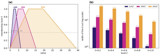
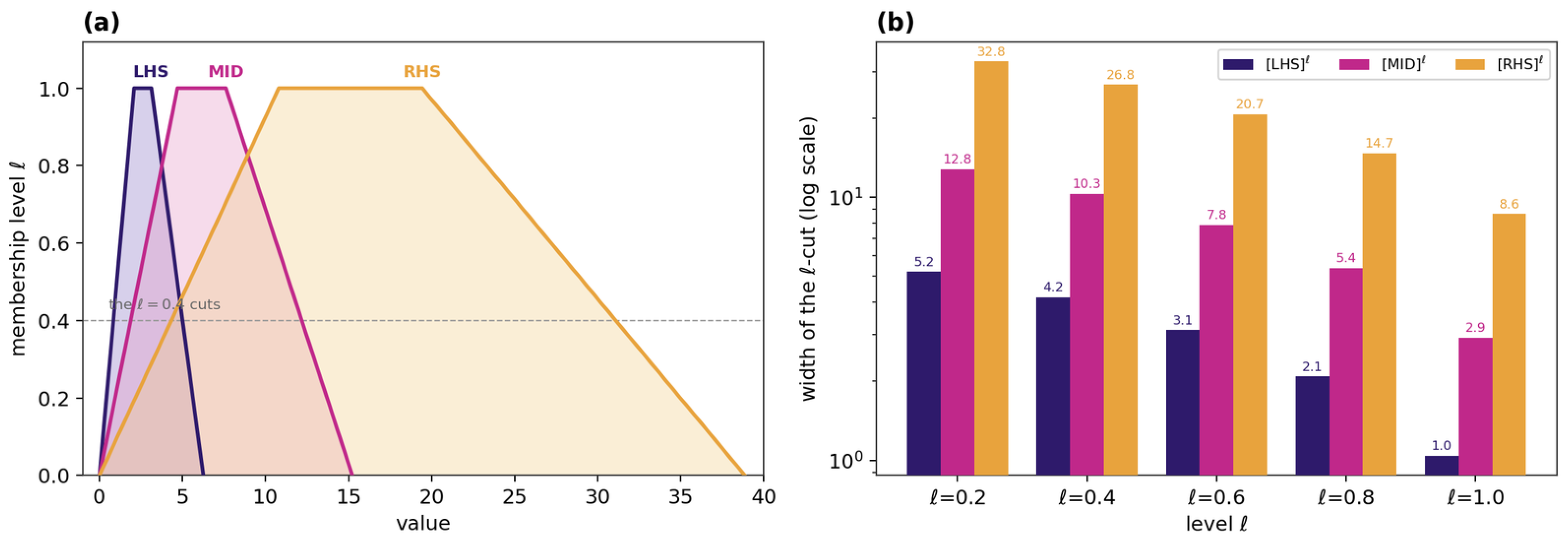
Two features of Table 1 and Figure 1 are worth noting. The cuts are nested, that is, as ℓ is increased from $0.2$ to 1 each, ${\left[\mathrm{MID}\right]}^{\ell }\to$ interval shrinks, e.g., ${\left[\mathrm{MID}\right]}^{\ell }={\left[H\right]}^{\ell }$, where H is a smaller interval. $[0.9381,13.7019]$ to $[4.6905,7.6121]$, in accordance with Definition 14. The width of the three cuts is not proportional, that is, at $\ell =0.2$ the width of ${\left[\mathrm{RHS}\right]}^{\ell }$ is about $32.8$ against about $5.2$ for ${\left[\mathrm{LHS}\right]}^{\ell }$, Thus, the uncertainty at each stage gets compounded along the chain when it is represented by fuzzy data. It can’t be seen on a crisp depiction for which all three are genuinely fuzzy effects; it cannot be seen on a crisp representation since the cuts are points that are isolated.

Figure 1. The ℓ-cuts of the three terms of the Hermite–Hadamard chain. (a) The membership functions of LHS, MID, and RHS as fuzzy numbers, with their supports shaded; the shaded regions overlap where the three fuzzy numbers share values, which is a genuine feature of the data (each curve is distinctly colored and outlined) rather than a rendering artifact, and does not impair legibility. The dashed horizontal line marks the $\ell =0.4$ cut used elsewhere in the discussion. (b) The width of the ℓ-cut of each term at five confidence levels $\ell \in \{0.2,0.4,0.6,0.8,1.0\}$, on a logarithmic vertical scale.

5.2. Numerical Illustration of the Hermite–Hadamard Chain (Theorem 1)

We first check the three-term chain $\mathrm{LHS}⪯\mathrm{MID}⪯\mathrm{RHS}$ of (22), where

$$\begin{array}{cc}\hfill \mathrm{LHS}& =\frac{1}{2}f\left({\left(\frac{{\mu }^p+{\nu }^p}{2}\right)}^{1/p}\right)E_{\alpha ,\beta +1}^{\rho }\left(\lambda \right),\hfill \\ \hfill \mathrm{MID}& ={\displaystyle \frac{{\left(\frac{e}{2}\right)}^{s/2}}{2{({\nu }^p-{\mu }^p)}^{\beta }}}\left[{\mathfrak{M}}_{\rho ,{\lambda }^{\prime },{\left({\mu }^p\right)}^{+}}^{\alpha ,\beta }{f}_p({\nu }^p,\ell )+{\mathfrak{M}}_{\rho ,{\lambda }^{\prime },{\left({\nu }^p\right)}^{-}}^{\alpha ,\beta }{f}_p({\mu }^p,\ell )\right],\hfill \\ \hfill \mathrm{RHS}& ={\left(\frac{e}{2}\right)}^s\left[f\left(\mu \right)+f\left(\nu \right)\right]E_{\alpha ,\beta +1}^{\rho }\left(\lambda \right).\hfill \end{array}$$

We independently recomputed $E_{\alpha ,\beta +1}^{\rho }\left(\lambda \right)$ by direct summation of its defining series at $\alpha =0.5$, $\beta =0.6$, $\rho =1$, $\lambda =0.5$ and confirmed $\mathrm{LHS}=2.0831$ and $\mathrm{RHS}=10.7934$ for $f\left(x\right)=x^2$ on $[\mu ,\nu ]=[1,2]$, in agreement with the first row of Table 2.

Table 2. Hermite–Hadamard chain of Theorem 1 for $f\left(x\right)=x^2$ under a joint variation of $(\alpha ,\beta ,s)$, with $p=1$, $\rho =1$, $\lambda =0.5$ and $[\mu ,\nu ]=[1,2]$.

$\mathit{\alpha }$	$\mathit{\beta }$	s	LHS	MID	RHS	RHS−LHS
0.5	0.6	0.5	2.0831	4.6905	10.7934	8.7103
0.6	0.7	0.6	1.9296	4.4034	10.3098	8.3802
0.8	0.9	0.7	1.6373	3.7846	9.0205	7.3832
1.0	1.0	1.0	1.4596	3.5304	8.8170	7.3574

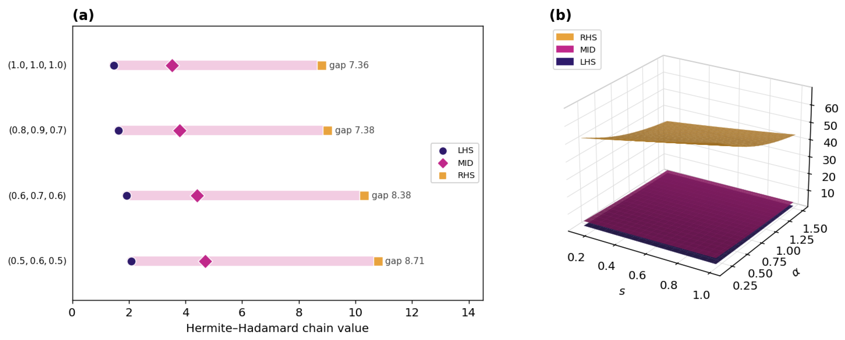
Table 2 reports the chain for $f_1\left(x\right)=x^2$ a joint variation of $(\alpha ,\beta ,s)$. In every row the ordering is preserved, and the gap $\mathrm{RHS}-\mathrm{LHS}$ contracts monotonically as the parameters increase towards unity.

Table 2 only checks four isolated parameter triples. Figure 2 extends the verification to the whole admissible region.

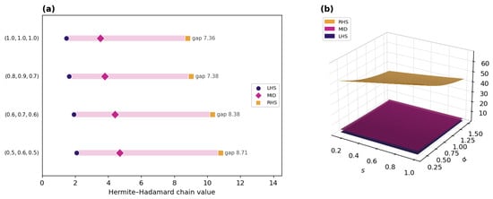
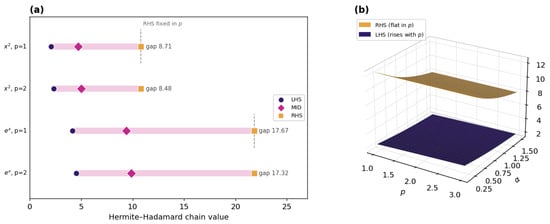
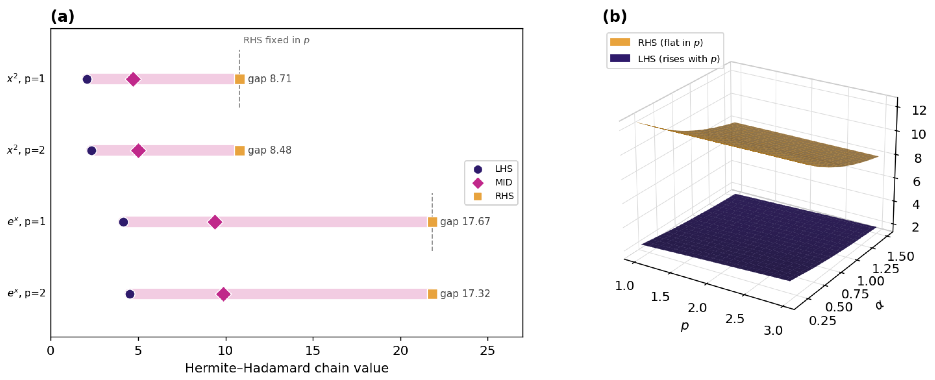
Figure 2. The Hermite–Hadamard chain of Theorem 1 for $f\left(x\right)=x^2$ ($p=1$, $\rho =1$, $\lambda =0.5$, $[\mu ,\nu ]=[1,2]$). (a) A range plot for the four parameter triples $(\alpha ,\beta ,s)$ of Table 2: for each triple, markers show $\mathrm{LHS}$ (∘), $\mathrm{MID}$ (⋄), and $\mathrm{RHS}$ (□), and the light pink bar spans the interval from $\mathrm{LHS}$ to $\mathrm{RHS}$, with its numerical width labeled as the gap. (b) The three quantities as surfaces over the $(\varphi ,s)$-grid (with $\varphi :=\alpha =\beta$); the $\mathrm{LHS}$ and $\mathrm{MID}$ surfaces lie close together near the bottom of the plot and the $\mathrm{RHS}$ surface is clearly separated above, which is a genuine feature of the data rather than a rendering overlap, since the three surfaces remain distinctly colored throughout.

Figure 2a shows the chain at the four parameter triples of Table 2: each range goes from $\mathrm{LHS}$ (∘) to As $\mathrm{MID}$ (⋄) to $\mathrm{RHS}$ (□), the gap narrows. $(\alpha ,\beta ,s)$ approach $(1,1,1)$. The ordering $\mathrm{LHS}\le \mathrm{MID}\le \mathrm{RHS}$ is a global property and not a local property. For isolated parameters, the plot of Figure 2b shows the coincidence at, The same three quantities as surfaces throughout the $(s,\alpha )$ domain ($\beta =0.6$): they never intersect.

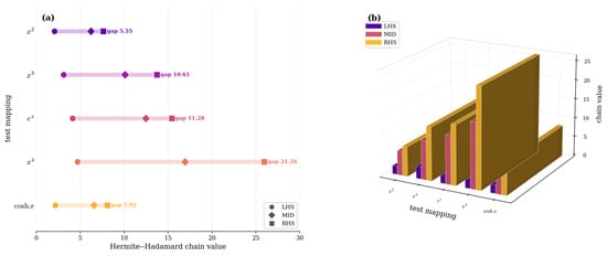
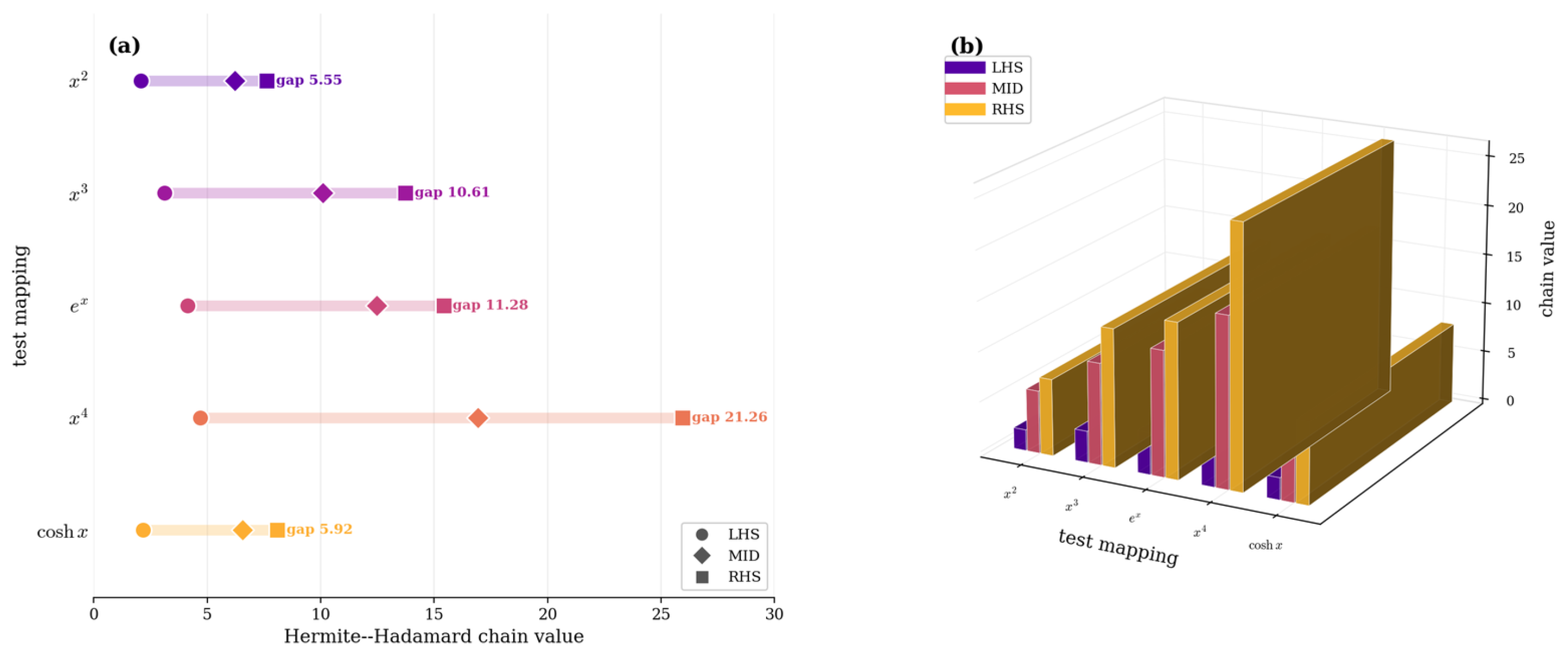
The chain for all five test functions at reference parameters $\alpha =0.5$ and $\beta =0.6$ and $s=0.5$ is given in Table 3 and the same data is plotted in Figure 3 to show that the result is independent of mapping.

Table 3. Hermite–Hadamard chain of Theorem 1 for five convex, non-negative test mappings, with $p=1$, $\alpha =0.5$, $\beta =0.6$, $s=0.5$.

Mapping f	LHS	MID	RHS	Chain
$x^2$	2.0831	4.6905	10.7934	✓
$x^3$	3.1247	7.6121	19.4282	✓
$e^x$	4.1492	9.3966	21.8186	✓
$x^4$	4.6870	12.7466	36.6977	✓
$coshx$	2.1779	4.9322	11.4524	✓

✓ indicates that the chain $\mathrm{LHS}\le \mathrm{MID}\le \mathrm{RHS}$ of (22) holds for that mapping.

Figure 3. The Hermite–Hadamard chain of Theorem 1 for the five test mappings ($p=1$, $\alpha =0.5$, $\beta =0.6$, $s=0.5$). (a) A range plot, one row per mapping, with markers for $\mathrm{LHS}$ (∘), $\mathrm{MID}$ (⋄), and $\mathrm{RHS}$ (□) joined by a bar whose color varies by row for visual distinction only, labeled with the numerical gap $\mathrm{RHS}-\mathrm{LHS}$. (b) The same three quantities as a grouped 3-D bar chart, one group of bars per mapping; the bars are shown in a 3-D perspective view, which is legible throughout since each of $\mathrm{LHS}$, $\mathrm{MID}$, $\mathrm{RHS}$ keeps its own color.

In Figure 3a, for each mapping, the range runs from $\mathrm{LHS}$ (∘) through $\mathrm{MID}$ (⋄) to $\mathrm{RHS}$ (□), the printed value being the gap $\mathrm{RHS}-\mathrm{LHS}$; and Figure 3b shows the same values as grouped columns. The ordering holds for polynomial, exponential, and hyperbolic growth alike.

5.3. Effect of the p-Convexity Parameter

An exceptional aspect of the present framework is the replacement of the classical midpoint by the MET-$(p,s)$ midpoint ${(\frac{{\mu }^p+{\nu }^p}{2})}^{1/p}$ of Definition 10. Table 4 compares $p=1$ with $p=2$ for the mappings $x^2$ and $e^x$.

Table 4. Influence of the p-convexity parameter on the chain of Theorem 1 ($\alpha =0.5$, $\beta =0.6$, $s=0.5$). The right-hand side depends only on the end-point values and is therefore independent of p.

Mapping f	p	LHS	MID	RHS
$x^2$	1	2.0831	4.6905	10.7934
$x^2$	2	2.3146	4.9982	10.7934
$e^x$	1	4.1492	9.3966	21.8186
$e^x$	2	4.4999	9.8682	21.8186

The term on the left-hand side increases, p whereas the right-hand side does not depend on p and hence the gap is decreasing and we get a tighter approximation. This is shown in Figure 4. So the option p provides us with a meaningful extra control over the sharpness of the restriction, as opposed to just recovering the convex case $p=1$.

Figure 4. Effect of the p-convexity parameter on the chain of Theorem 1 for $f\left(x\right)=x^2$ and $f\left(x\right)=e^x$ ($\beta =0.6$, $s=0.5$). (a) A range plot as in Figure 3a, with one row for each mapping at $p=1$ and $p=2$; the dashed vertical line marks the (fixed-in-p) $\mathrm{RHS}$ position for each mapping, so that the leftward shift of $\mathrm{LHS}$ and the narrowing gap as p increases from 1 to 2 can be read off directly. (b) The $\mathrm{LHS}$ and $\mathrm{RHS}$ surfaces over $(p,\varphi )$ (with $\varphi :=\alpha =\beta$), confirming that $\mathrm{RHS}$ is flat in p while $\mathrm{LHS}$ increases with p throughout the domain shown.

In Figure 4a the right-hand side (dashed line) is constant in p at $\alpha =0.5$ and increasing p from 1 to 2 increases the left-hand side (arrow) and decreases the gap. The left- and right-hand surfaces over $(p,\alpha )$ in Figure 4b are such that the right-hand surfaces are flat in p, and the left-hand ones rise with p over the whole domain.

5.4. Numerical Illustration of the Trapezoid-Type Error Bounds (Theorems 2–4)

In the present and the next two subsections we assume that the parameter $\beta$ is bigger than one, as required by the hypothesis of Lemma 1; see Remark 7. We compare the real deviation of

$$D=\left|{\displaystyle \frac{\zeta (\nu ,\mu )}{2}}{\int }_0^1\mathcal{K}\left(w\right)f^{\prime }\left(\mu +w\zeta (\nu ,\mu )\right)dw\right|,$$

obtained from the identity of Lemma 1, with $\mathcal{K}$ the kernel difference (41), against the three upper bounds $B_{4.1}$, $B_{4.2}$ and $B_{4.3}$ furnished by Theorems 2, 3 and 4, respectively. Here we take $p=1$, so that $\zeta (\nu ,\mu )={\nu }^1-{\mu }^1=\nu -\mu$ the general definitions use $\zeta (\nu ,\mu )={\nu }^p-{\mu }^p$, and $f_p=f$ at $p=1$, under which the invex domain $[\mu ,\mu +\zeta (\nu ,\mu \left)\right]$ collapses to $[\mu ,\nu ]=[1,2]$.

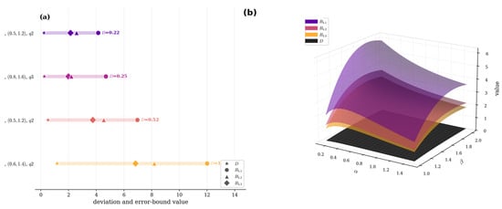
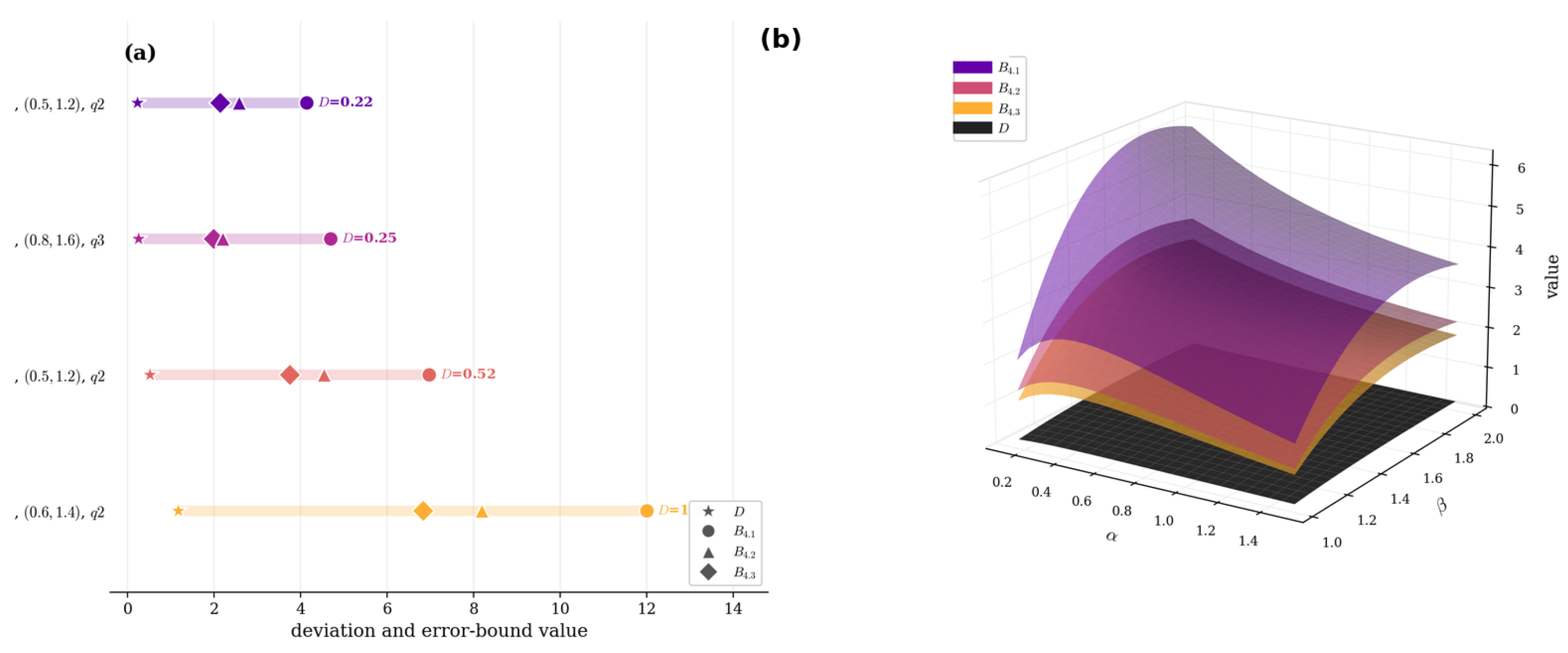
Table 5 gives the actual deviation D against the three trapezoid-type upper bounds $B_{4.1}$ (basic), $B_{4.2}$ (Hölder) and $B_{4.3}$ (power-mean) of Theorems 2–4, with $\mu =1$, $\nu =2$, $\rho =1$, $\lambda =0.5$ and $\zeta (\nu ,\mu )=\nu -\mu$. In accordance with Lemma 1, all configurations satisfy $\beta >1$. Table 5 and Figure 5 show that in every configuration the deviation is comfortably dominated by each of the three bounds, and that the power-mean bound $B_{4.3}$ is the tightest of the three.

Table 5. Actual deviation D against the three trapezoid-type upper bounds.

f	$\mathit{\alpha }$	$\mathit{\beta }$	q	D	${\mathit{B}}_{4.1}$	${\mathit{B}}_{4.2}$	${\mathit{B}}_{4.3}$
$x^2$	0.5	1.2	2.0	0.2246	4.1379	2.5772	2.1318
$x^2$	0.8	1.6	3.0	0.2510	4.6926	2.1957	1.9851
$e^x$	0.5	1.2	2.0	0.5165	6.9705	4.5371	3.7531
$x^3$	0.6	1.4	2.0	1.1629	11.9901	8.1869	6.8297

Figure 5. Actual deviation D against the three trapezoid-type upper bounds of Theorems 2–4. (a) A range plot for four parameter configurations $(\alpha ,\beta ,q)$: D (★) sits far to the left of $B_{4.3}$ (⋄), $B_{4.2}$ (▵), and $B_{4.1}$ (∘) in each row, with the numerical value of D labeled. (b) The same four quantities as surfaces over $\alpha \in (0.15,1.5]$ and $\beta \in (1,2]$ for $f\left(x\right)=x^2$ with $q=2$; the D surface (black, flat near zero) lies below all three bound surfaces throughout.

Figure 5a Table 5 has four configurations: D (★) is located far to the left of $B_{4.1}$ (∘), $B_{4.2}$ (▵), and $B_{4.3}$ (⋄) in each row. Figure 5b The deviation surface sits below all three bound surfaces throughout, and $B_{4.3}\le B_{4.2}\le B_{4.1}$ everywhere. These four quantities are the same as surfaces over $\alpha \in (0.15,1.5]$ and $\beta \in (1,2]$ for $f\left(x\right)=x^2$ with $q=2$.

5.5. Behaviour of the Three Bounds

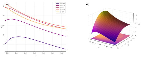
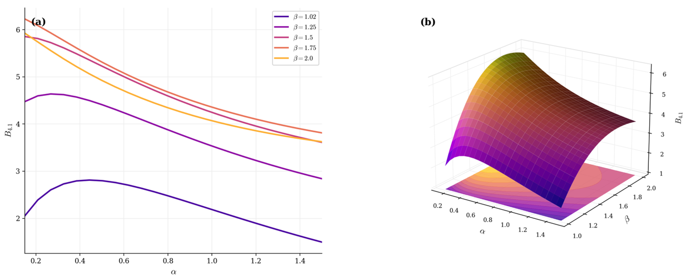
Figure 6 shows the bound $B_{4.1}$ of Theorem 2 for $f\left(x\right)=x^2$ with $\alpha \in (0.15,1.5]$ and $\beta \in (1,2]$. The bound decreases monotonically with increase of fractional order $\alpha$. At $\beta =1.5$ it decreases from about $5.86$ at $\alpha =0.15$ to about $3.61$ at $\alpha =1.5$. Its dependence on $\beta$ is non-monotonic, rising with the deviation of $\beta$ from 1, reaching its greatest values near $\beta \approx 1.75$ (∼6.23 for $\alpha =0.15$) and then falling again as $\beta$ approaches 2. The bound is only of the order of about $1.50$ to $6.23$ in the region.

Figure 6. The trapezoid-type upper bound $B_{4.1}$ of Theorem 2 for $f\left(x\right)=x^2$ with $\alpha \in (0.15,1.5]$ and $\beta \in (1,2]$. (a) $B_{4.1}$ against $\alpha$ for five fixed values of $\beta$. (b) $B_{4.1}$ as a surface over $(\alpha ,\beta )$, colored by its value on the same scale as the surface; the shaded panel beneath is a contour projection of the same surface, shown for orientation.

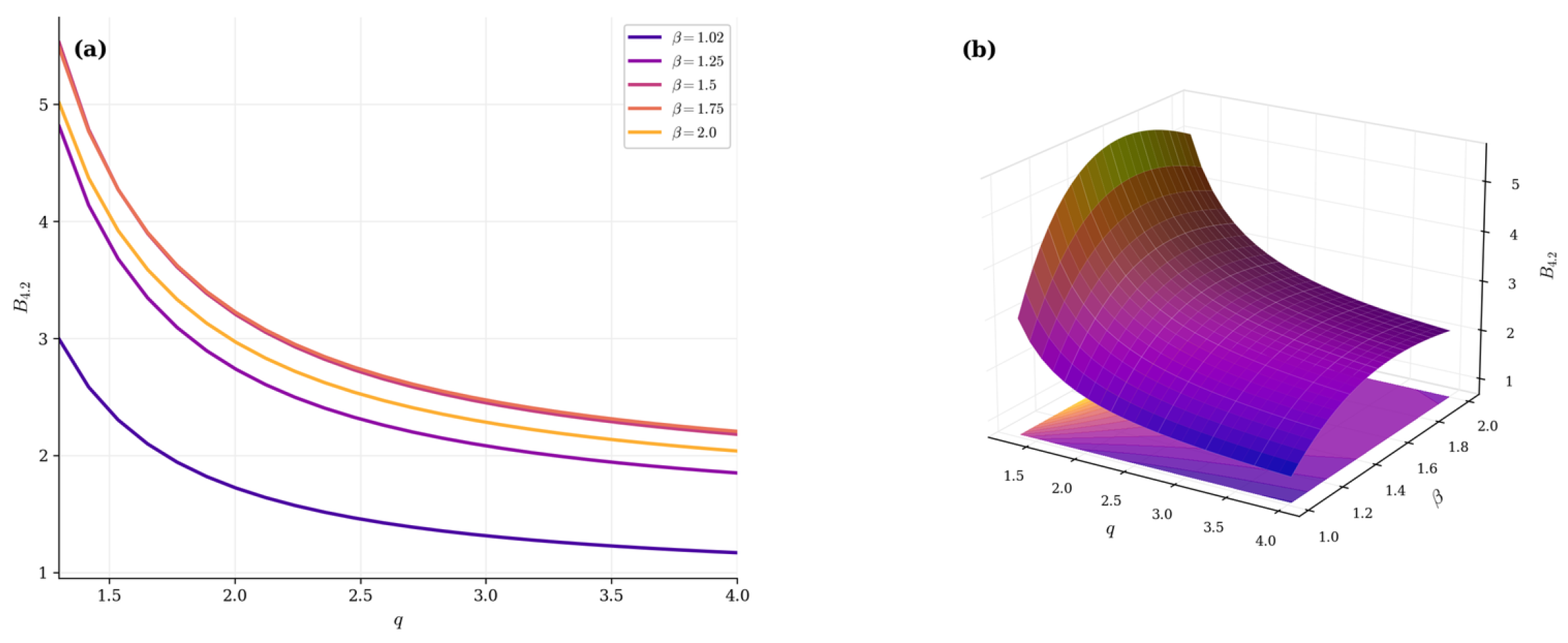
For $f\left(x\right)=x^2$, with $\rho =1$, $\lambda =0.5$ and $[\mu ,\nu ]=[1,2]$. Figure 6a Sections at five values of $\beta$, showing the decay in $\alpha$. and Figure 6b displays the corresponding surface over $\alpha \in (0.15,1.5]$ and $\beta \in (1,2]$,with its floor-projected contour map. The Holder-type bound $B_{4.2}$ in Theorem 3 is shown in Figure 7 as a function of the exponent $q\in (1.3,4]$ and of $\beta \in (1,2]$, for $\alpha =0.5$ fixed. The bound decreases monotonically in q; at $\beta =1.5$, it decreases from around $5.53$ at $q=1.3$ to about $2.18$ at $q=4$. As the kernel difference $\mathcal{K}$ of (41) is bounded on $[0,1]$ for $\beta >1$, in Theorem 3 the quantity ${\left({\int }_0^1{\left|\mathcal{K}\left(w\right)\right|}^{r}dw\right)}^{1/r}$ is finite for high values of the conjugate exponent $r=q/(q-1)$, that is, when q goes to 1. Thus there is no practical need to restrict q, as the Hölder-type estimate is stable across the complete permissible range.

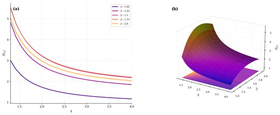
Figure 7. The Hölder-type bound $B_{4.2}$ of Theorem 3. (a) $B_{4.2}$ against q for five fixed values of $\beta$. (b) $B_{4.2}$ as a surface over $(q,\beta )$, colored by its value on the same scale as the surface; the shaded panel beneath is a contour projection of the same surface, shown for orientation.

For $f\left(x\right)=x^2$, with $\alpha =0.5$, $\rho =1$, $\lambda =0.5$ and $[\mu ,\nu ]=[1,2]$, Figure 7a sections are plotted at five values of $\beta$, illustrating the monotone decrease of q. The power-mean bound $B_{4.3}$ of Theorem 4 reduces as both $\alpha$ and q increase: at $\beta =1.5$, it drops from around $4.28$ at $\alpha =0.15$, $q=1.3$ to roughly $1.40$ at $\alpha =1.5$, $q=4$. It is smooth all over. This illustrates the fact that this numerically well-behaved approximation is obtained by the power-mean inequality used in the proof of Theorem 4.

5.6. Comparison of Three Bounds of Trapezoid Type

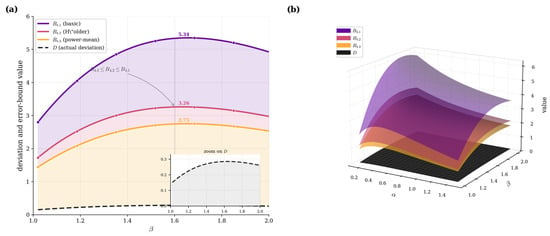
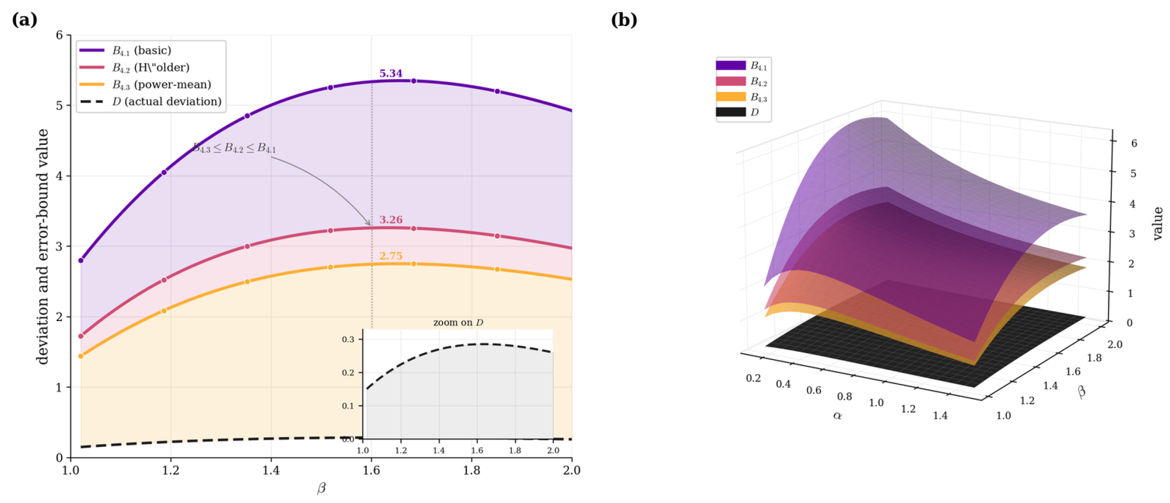
In Figure 8, all three bounds are compared with the actual deviation D at $\alpha =0.5$ and $q=2$. Three observations stand out. First, the deviation D stays well within all three bounds throughout, ranging only between about $0.15$ and $0.29$. Second, the ordering $B_{4.3}\le B_{4.2}\le B_{4.1}$ holds throughout; at $\beta =1.6$, for instance, the three bounds never drop below about $1.44$ and take the values approximately $2.75$, $3.26$, and $5.34$, respectively. Third, the deviation follows the same qualitative pattern in $\beta$ as the three bounds: all four quantities decrease as $\beta$ moves away from 1 toward 2.

Figure 8. Comparison of the three trapezoid-type bounds against the actual deviation D, for $f\left(x\right)=x^2$ with $q=2$, $\rho =1$, $\lambda =0.5$. (a) Against $\beta \in (1,2]$ at $\alpha =0.5$: the deviation (dashed) stays far below all three bounds, and $B_{4.3}$ is uniformly the tightest; the shaded bands between curves and the inset zoom on D are for visual clarity only and do not affect legibility. (b) The same four quantities as surfaces over $(\alpha ,\beta )$ illustrating that the ordering holds over the plotted region; the surfaces are shown with partial transparency so that all four remain visible where they overlap.

5.7. Comparison with Existing Results

We close this section by finding the results of the paper with respect to the available literature, first structurally and then numerically as well.

Special cases. Since ${\left(\rho \right)}_0=1$, the defining series of the generalized Mittag–Leffler kernel gives $E_{\alpha ,\beta }^{\rho }\left(0\right)=1/\mathrm{\Gamma }\left(\beta \right)$, so that for $\lambda =0$ the Prabhakar operators of Definition 18 collapse to the Riemann–Liouville fractional integrals,

$${\mathfrak{M}}_{\rho ,0,a^{+}}^{\alpha ,\beta }f\left(x\right)=\mathrm{\Gamma }\left(\beta \right)J_{a^{+}}^{\beta }f\left(x\right),{\mathfrak{M}}_{\rho ,0,b^{-}}^{\alpha ,\beta }f\left(x\right)=\mathrm{\Gamma }\left(\beta \right)J_{b^{-}}^{\beta }f\left(x\right).$$

Table 6 records the classes and operators recovered from Definition 10 and Theorem 1 for particular values of the parameters. In this Riemann–Liouville limit the chain of Theorem 1 is directly comparable with the fractional Hermite–Hadamard inequalities obtained for generalized preinvex classes [43,44,45].

Table 6. Classes and operators recovered from Definition 10 and Theorem 1 for particular values of the parameters.

Parameters	Recovered Object
$p=1$, $s=1$	modified exponential trigonometric convexity (Definition 9)
$s=1$	modified exponential trigonometric p-convexity
$p=1$	modified exponential trigonometric s-convexity
$\lambda =0$	Riemann–Liouville fractional integrals
$\lambda =0$, $\beta =1$	the ordinary Riemann integral
$f_{\ast }=f^{\ast }=f$	the crisp (real-valued) theory

The advantage of MET-$(p,s)$-convexity is generality rather than sharpness, and this can be illustrated precisely. Consider $f\left(x\right)=\sqrt{x}$ on $[\mu ,\nu ]=[1,2]$: this function is concave, so the classical Hermite–Hadamard inequality does not apply to it, and the three quantities run in the wrong order,

$$f\left({\displaystyle \frac{\mu +\nu }{2}}\right)=1.2247\ge {\displaystyle \frac{1}{\nu -\mu }}{\int }_{\mu }^{\nu }f=1.2190\ge {\displaystyle \frac{f\left(\mu \right)+f\left(\nu \right)}{2}}=1.2071.$$

Nevertheless $\sqrt{x}$ is MET-$(1,1)$-convex on $[1,2]$, so Theorem 1 does apply, and it returns valid bounds: at $\lambda =0$, $\beta =1$, $p=1$, $s=1$ the chain (22) reads $0.6124\le 1.4211\le 3.2813$, and at the reference parameters $\alpha =0.5$, $\beta =0.6$, $s=0.5$, $\lambda =0.5$ it reads $1.1339\le 2.4352\le 5.2115$.

Price of the generality. On a mapping to which both theories apply, the classical inequality is of course the sharper one. For $f\left(x\right)=x^2$ on $[\mu ,\nu ]=[1,2]$, the classical Hermite–Hadamard chain gives $1.1250\le 1.1667\le 1.2500$, whereas Theorem 1 with $\lambda =0$, $\beta =1$, $p=1$, $s=1$ gives $1.1250\le 2.7203\le 6.7957$. The left-hand sides agree (since $E_{\alpha ,2}^{\rho }\left(0\right)=1$), while the middle and right-hand terms of (22) are larger: this is the price paid for generality, since the weights ${[sin{\displaystyle \frac{\pi t}{2}}{e}^{1-t}]}^s$ and ${[cos{\displaystyle \frac{\pi t}{2}}{e}^t]}^s$ of Definition 10 sum to more than one. In short, the class of admissible mappings was enlarged to include non-convex functions such as $\sqrt{x}$ at the cost of looser constants; Theorem 1 should therefore be read as extending the range of applicability of the Hermite–Hadamard-type chain, not as improving the classical bound on the convex mappings for which the classical inequality already applies.

6. Conclusions

In this paper, we refined the Hermite-Hadamard and trapezoid type inequalities with the newly described MET-$(p,s)$-fuzzy convex function and implementation of Prabhakar fuzzy fractional operators. The proposed framework extends and generalizes several existing convexity models, widening the class of admissible mappings beyond ordinary convexity. The inequalities derived here provide computable lower and upper bounds for Prabhakar fractional means in applications involving fractional models with an uncertain modeling domain expressed in fuzzy intervals. They are useful because they only require the model data at the endpoints. Moreover, we presented numerical illustrations of our main results and also checked the behavior for different values of parameters. We conclude that most of these inequalities can be further extended to other fuzzy-interval-valued mappings and fuzzy fractional operators, together with a discussion of their physical interpretations and applications. In future work, the study of Ostrowski, Simpson, Fej’er, and Chebyshev-type inequalities will consider the midpoint parametric values of $s<1$, the extension case for $\beta \le 1$, and also promote the multi-index fractional operators.

The results are established under $\rho >0$, $\lambda \ge 0$, which guarantees a nonnegative Prabhakar kernel but excludes sign-changing kernels; the main chain (22) is a generalization in the sense of admitting a wider class of mappings, not a numerically sharper bound on the classical convex class (Section 5.7); and the trapezoid-type bounds of Theorems 2–4 require $\beta >1$. Extending the theory to $\lambda <0$, to $p<0$, and to $0<\beta \le 1$ is left for future work, together with a systematic theorem-by-theorem numerical comparison against the closest existing exponential-trigonometric, p-convex, and Prabhakar fuzzy fractional inequalities.

References

- Hardy, G.H.; Littlewood, J.E.; Pólya, G. Inequalities; Cambridge University Press: Cambridge, UK, 1952. [Google Scholar]
- Niculescu, C.; Persson, L.E. Convex Functions and Their Applications; Springer: New York, NY, USA, 2006; Volume 23. [Google Scholar]
- Mubeen, S.; Ali, R.S.; Nayab, I.; Rahman, G.; Nisar, K.S.; Baleanu, D. Some generalized fractional integral inequalities with nonsingular function as a kernel. AIMS Math. 2021, 6, 3352–3377. [Google Scholar] [CrossRef] [Scilit]
- Meftah, B.; Boulares, H.; Shafqat, R.; Ben Makhlouf, A.; Benaicha, R. Some new fractional weighted Simpson type inequalities for functions whose first derivatives are convex. Math. Probl. Eng. 2023, 2023, 9945588. [Google Scholar] [CrossRef] [Scilit]
- Butt, S.I.; Bakula, K.; Pečarić, M.; Pečarić, J. Jensen–Grüss inequality and its applications for the Zipf–Mandelbrot law. Math. Methods Appl. Sci. 2021, 44, 1664–1673. [Google Scholar] [CrossRef] [Scilit]
- Butt, S.I.; Nadeem, M.; Qaisar, S.; Akdemir, A.O.; Abdeljawad, T. Hermite–Jensen–Mercer type inequalities for conformable integrals and related results. Adv. Differ. Equ. 2020, 2020, 501. [Google Scholar] [CrossRef] [Scilit]
- Nwaeze, E.R.; Khan, M.A.; Chu, Y.M. Fractional inclusions of the Hermite–Hadamard type for m-polynomial convex interval-valued functions. Adv. Differ. Equ. 2020, 2020, 507. [Google Scholar] [CrossRef] [Scilit]
- Tariq, M.; Ahmad, H.; Budak, H.; Sahoo, S.K.; Sitthiwirattham, T.; Reunsumrit, J. A comprehensive analysis of Hermite–Hadamard type inequalities via generalized preinvex functions. Axioms 2021, 10, 328. [Google Scholar] [CrossRef] [Scilit]
- Hudzik, H.; Maligranda, L. Some remarks on s-convex functions. Aequ. Math. 1994, 48, 100–111. [Google Scholar] [CrossRef] [Scilit]
- Gao, W.; Kashuri, A.; Butt, S.I.; Tariq, M.; Aslam, A.; Nadeem, M. New inequalities via n-polynomial harmonically exponential type convex functions. AIMS Math. 2020, 5, 6856–6873. [Google Scholar] [CrossRef] [Scilit]
- Mohan, S.R.; Neogy, S.K. On invex sets and preinvex functions. J. Math. Anal. Appl. 1995, 189, 901–908. [Google Scholar] [CrossRef] [Scilit]
- Kadakal, M.; İşcan, İ.; Kadakal, H.; Bekar, K. On improvements of some integral inequalities. Honam Math. J. 2021, 43, 441–452. [Google Scholar]
- Moumen, A.; Boulares, H.; Meftah, B.; Shafqat, R.; Alraqad, T.; Ali, E.E.; Khaled, Z. Multiplicatively Simpson type inequalities via fractional integral. Symmetry 2023, 15, 460. [Google Scholar] [CrossRef] [Scilit]
- Boulares, H.; Meftah, B.; Moumen, A.; Shafqat, R.; Saber, H.; Alraqad, T.; Ali, E.E. Fractional multiplicative Bullen-type inequalities for multiplicative differentiable functions. Symmetry 2023, 15, 451. [Google Scholar] [CrossRef] [Scilit]
- Rashid, S.; İşcan, İ.; Baleanu, D.; Chu, Y.M. Generation of new fractional inequalities via n-polynomials s-type convexity with applications. Adv. Differ. Equ. 2020, 2020, 1–20. [Google Scholar] [CrossRef] [Scilit]
- Zahra, M.; Chu, Y.M.; Farid, G. Refinements of some integral inequalities for convex functions. J. Math. 2020, 2020, 8878342. [Google Scholar] [CrossRef] [Scilit]
- Saleem, M.S.; Chu, Y.M.; Jahangir, N.; Akhtar, H.; Jung, C.Y. On generalized strongly convex functions of higher order. J. Math. 2020, 2020, 8381431. [Google Scholar] [CrossRef] [Scilit]
- Hanson, M.A. On sufficiency of the Kuhn–Tucker conditions. J. Math. Anal. Appl. 1981, 80, 545–550. [Google Scholar] [CrossRef] [Scilit]
- Ben-Israel, A.; Mond, B. What is invexity? ANZIAM J. 1986, 28, 1–9. [Google Scholar] [CrossRef] [Scilit]
- Antczak, T. Mean value in invexity analysis. Nonlinear Anal. Theory Methods Appl. 2005, 60, 1473–1484. [Google Scholar] [CrossRef] [Scilit]
- Noor, M.A. Variational-like inequalities. Optimization 1994, 30, 323–330. [Google Scholar] [CrossRef] [Scilit]
- Farajzadeh, A.; Noor, M.A.; Noor, K.I. Vector nonsmooth variational-like inequalities and optimization problems. Nonlinear Anal. Theory Methods Appl. 2009, 71, 3471–3476. [Google Scholar] [CrossRef] [Scilit]
- Kadakal, H. Hermite–Hadamard type inequalities for trigonometrically convex functions. Sci. Stud. Res. Ser. Math. Inform. 2018, 28, 19–28. [Google Scholar]
- Khan, M.B.; Mohammed, P.O.; Noor, M.A.; Hamed, Y.S. New Hermite–Hadamard inequalities in fuzzy-interval fractional calculus and related inequalities. Symmetry 2021, 13, 673. [Google Scholar] [CrossRef] [Scilit]
- Nayab, I.; Mubeen, S.; Ali, R.S.; Zahoor, F.; Awadalla, M.; Elamin, A.E.A.M.A. Novel fractional inequalities measured by Prabhakar fuzzy fractional operators pertaining to fuzzy convexities and preinvexities. AIMS Math. 2024, 9, 17696–17715. [Google Scholar] [CrossRef] [Scilit]
- Hermite–Hadamard-type inequalities for h-Godunova–Levin convex fuzzy interval-valued functions via Riemann–Liouville fractional q-integrals. Fractal Fract. 2025, 9, 578. [CrossRef] [Scilit]
- The Hadamard and generalized fractional integral fuzzy-number-valued operators for mappings of one and two variables, and their related fuzzy number inequalities. Fractal Fract. 2026, 10, 228. [CrossRef] [Scilit]
- Demir Budak, K.; Gürbüz, M. Modified exponential trigonometric convex functions and some integral inequalities. Turk. J. Inequal. 2024, 8, 60–72. [Google Scholar]
- Zhang, K.S.; Wan, J.P. p-convex functions and their properties. Pure Appl. Math. 2007, 23, 130–133. [Google Scholar] [CrossRef] [Scilit]
- Park, C.; Chu, Y.M.; Saleem, M.S.; Jahangir, N.; Rehman, N. On n-polynomial p-convex functions and some related inequalities. Adv. Differ. Equ. 2020, 2020, 666. [Google Scholar] [CrossRef] [Scilit]
- Butt, S.I.; Budak, H.; Tariq, M.; Nadeem, M. Integral inequalities for n-polynomial s-type preinvex functions with applications. Math. Methods Appl. Sci. 2021, 44, 11006–11021. [Google Scholar] [CrossRef] [Scilit]
- Toader, G.H. Some generalizations of the convexity. In Proceedings of the Colloquium on Approximation and Optimization, Cluj-Napoca, Romania, 25–27 October 1984; Volume 329, pp. 1–338. [Google Scholar]
- Latif, M.A.; Shoaib, M. Hermite–Hadamard type integral inequalities for differentiable m-preinvex and (α,m)-preinvex functions. J. Egypt. Math. Soc. 2015, 23, 236–241. [Google Scholar] [CrossRef] [Scilit]
- Deng, Y.; Kalsoom, H.; Wu, S. Some new quantum Hermite–Hadamard-type estimates within a class of generalized (s,m)-preinvex functions. Symmetry 2019, 11, 1283. [Google Scholar] [CrossRef] [Scilit]
- Toplu, T.; Kadakal, M.; İşcan, İ. On n-polynomial convexity and some related inequalities. AIMS Math. 2020, 5, 1304–1318. [Google Scholar] [CrossRef] [Scilit]
- Kadakal, M.; İşcan, İ.; Agarwal, P.; Jleli, M. Exponential trigonometric convex functions and Hermite–Hadamard type inequalities. Math. Slovaca 2021, 71, 43–56. [Google Scholar] [CrossRef] [Scilit]
- Garrappa, R.; Mainardi, F.; Maione, G. Models of dielectric relaxation based on completely monotone functions. Fract. Calc. Appl. Anal. 2016, 19, 1105–1160. [Google Scholar] [CrossRef] [Scilit]
- Zadeh, L.A. Fuzzy sets. Inf. Control 1965, 8, 338–353. [Google Scholar] [CrossRef] [Scilit]
- Goetschel, R.; Voxman, W. Elementary fuzzy calculus. Fuzzy Sets Syst. 1986, 18, 31–43. [Google Scholar] [CrossRef] [Scilit]
- Kaleva, O. Fuzzy differential equations. Fuzzy Sets Syst. 1987, 24, 301–317. [Google Scholar] [CrossRef] [Scilit]
- Giusti, A.; Colombaro, I.; Garra, R.; Garrappa, R.; Polito, F.; Popolizio, M.; Mainardi, F. A practical guide to Prabhakar fractional calculus. Fract. Calc. Appl. Anal. 2020, 23, 9–54. [Google Scholar] [CrossRef] [Scilit]
- Górska, K.; Horzela, A.; Lattanzi, A.; Pogány, T.K. On the complete monotonicity of the three parameter generalized Mittag–Leffler function (−x). arXiv 2018, arXiv:1811.10441. [Google Scholar]
- Barani, A.; Ghazanfari, A.G.; Dragomir, S.S. Hermite–Hadamard inequality for functions whose derivatives absolute values are preinvex. J. Inequal. Appl. 2012, 2012, 247. [Google Scholar] [CrossRef] [Scilit]
- Du, T.S.; Liao, J.G.; Li, Y.J. Properties and integral inequalities of Hadamard–Simpson type for the generalized (s,m)-preinvex functions. J. Nonlinear Sci. Appl. 2016, 9, 3112–3126. [Google Scholar] [CrossRef] [Scilit]
- Du, T.S.; Liao, J.; Chen, L.; Awan, M.U. Properties and Riemann–Liouville fractional Hermite–Hadamard inequalities for the generalized (α,m)-preinvex functions. J. Inequal. Appl. 2016, 2016, 306. [Google Scholar] [CrossRef] [Scilit]
Disclaimer/Publisher’s Note: The statements, opinions and data contained in all publications are solely those of the individual author(s) and contributor(s) and not of MDPI and/or the editor(s). MDPI and/or the editor(s) disclaim responsibility for any injury to people or property resulting from any ideas, methods, instructions or products referred to in the content. |
© 2026 by the authors. Licensee MDPI, Basel, Switzerland. This article is an open access article distributed under the terms and conditions of the Creative Commons Attribution (CC BY) license.