Modeling Saudi Price Index Using a New Bivariate Family of Distributions

Abstract

The price index of daily commodities is an important indicator of inflation in a country. Adequate modeling of the price index is useful for efficient economic decision-making. Since the exact modeling of the price index is impossible, probabilistic modeling is a suitable alternative for this. The change in the price index of various commodities at different time points is usually dependent, and hence joint modeling is a suitable solution. In this paper, a new family of distributions is proposed for joint modeling of the price index of various Saudi commodities at two different time points and is named as Darwish Bivariate Family of Distributions (DBFDs). Some necessary properties of the family are presented, and some dependence measures are also computed. Conditional distributions for the proposed family are investigated alongside the method for random data generation from any member of the proposed family. The parameter estimation for the proposed family is discussed in general. A specific member of the family, namely the Darwish Bivariate Log-logistic (DBLL) distribution, is studied in detail. Some important properties of the DBLL distribution are presented. The DBLL distribution is used to model the price index of various Saudi commodities. It is found that the proposed DBLL distribution provides a better fit to model the price index in comparison with the other models used in the study.

1. Introduction

The economic stability of a country hugely depends upon the inflation rate. A country with a lower inflation rate is supposed to be economically stable. The credibility of the economic status of a country also depends upon the credibility of its banks in settling the import and export credits. The future prediction of the price index (PI) is an important factor in efficient economic planning for banks and for the country. The PI follows a random pattern; hence, some probabilistic methods are required. Probability distributions are being efficiently used to model random phenomena in many areas of life, and economic variables are not an exception. The PI can be effectively modeled by using some suitable probability distributions.

Several situations arise where one is required to jointly model two or more than two random phenomena. In such cases, some bivariate or multivariate distributions are required. Various bivariate distributions are available in the literature, but the everyday complexity arising from the data has limited the use of the available bivariate distributions. Thus, the quest continues to propose new bivariate or multivariate probability distributions. The development of bivariate distributions is not an easy task, and various methods have been proposed by various researchers to obtain a bivariate or multivariate distribution from the given univariate marginals.

A classical method of generating bivariate and multivariate distributions was proposed by [1] and is used to obtain a bivariate logistic distribution [2]. The method of Gumbel has been extended by various researchers to propose new methods of generating bivariate distributions [3,4]. A comprehensive coverage of the extensions of the Gumbel method is also given by some authors [5,6]. The method proposed by Gumbel and its extensions provide the baseline distributions as the marginals and is broadly known as copula, see [6].

In recent years, some other methods have been proposed to generate bivariate distributions from the univariate distributions. These methods do not provide the univariate distributions as marginals but instead provide some univariate family of distributions as the marginals. One such method provides the beta family of distributions as marginals [7], and another provides the transmuted family of distributions as marginals [8]. A general method of obtaining new bivariate families of distributions is available [9], and its simpler version was used to obtain a new family of distributions for joint modeling of various economic and demographic variables by [10]. The family of distributions proposed by [8] has been used by [11] to obtain a new bivariate family of distributions. The marginal distributions in the bivariate family of distributions by [11] turned out to be the exponentiated distributions.

In this paper, a new family of distributions is obtained for joint modeling of two variables. Some important material and methods are discussed in the following.

2. Material and Methods

In recent years, the developments in families of distributions have revolutionized the modeling of complex data. A general method of developing univariate families of distributions is the T-X method [12], which has been used by various authors to propose new families of distributions, see [13]. A bivariate extension of this method has been proposed by [9], which utilizes any bivariate distribution as a generator to propose a new bivariate family of distributions. The joint “cumulative distribution function” (cdf) of this family of distributions is

$$F_{1,2}\left(w,z\right)={\displaystyle {\int }_{c_2}^{{\zeta }_2\left[G_2\left(z\right)\right]}{\displaystyle {\int }_{c_1}^{{\zeta }_1\left[G_1\left(w\right)\right]}r\left(u,v\right)\mathrm{d}u\mathrm{d}v}} ; c_1<u<d_1 ; c_2<v<d_2,$$

(1)

where G₁(w) and G₂(z) are cdfs of the baseline distributions, ζ₁[G₁(w)] and ζ₂[G₂(z)] are any functions of G₁(w) and G₂(z) such that ζ₁(0)→c₁, ζ₁(1)→d₁, ζ₂(0)→c₂ and ζ₂(1)→d₂, and r(u,v) is any bivariate distribution with support on [c₁,d₁] × [c₂,d₂]. A simpler version of (1), for random variables that are closed within [0, 1], is given by [8] as

$$F_{1,2}\left(w,z\right)={\displaystyle {\int }_0^{G_2\left(z\right)}{\displaystyle {\int }_0^{G_1\left(xw\right)}r\left(u,v\right)\mathrm{d}u\mathrm{d}v}}.$$

(2)

The Gumbel bivariate distribution [1] is obtained by using

$$r\left(u,v\right)=1+\alpha \left(1-2u\right)\left(1-2v\right) ; 0\le \left(u,v\right)\le 1$$

in (2). The bivariate beta family of distributions is obtained by [7] by using the bivariate beta distribution of [14] in (2). A bivariate transmuted family of distributions is obtained by [8] by using the following r(u,v) in (2)

$$r\left(u,v\right)=1+{\alpha }_1\left(1-2u\right)+{\alpha }_2\left(1-2v\right)+2{\alpha }_3\left(1-u-v\right) ; 0\le \left(u,v\right)\le 1.$$

The bivariate family of distributions given in (2) is a cornerstone in developing new families of bivariate distributions such that the marginal families are some well-known families of distributions. A new family of distributions is obtained in the following section by using (2).

3. New Family of Distributions

In this section, a new bivariate family of distributions will be obtained that will be capable of modeling more complex data. Some useful properties of the proposed family of distributions will also be presented. The new bivariate family of distributions is obtained in the following.

Several situations arise where the modeling of bivariate data requires some complex distributions. In such situations, we require distributions that contain some higher powers of the cdf. In the following, a new bivariate family of distributions will be obtained that will be capable of modeling some complex data. Various generators r(u,v) can be used in (2) to obtain new families of distributions. In this paper, the following generator

$$r\left(u,v\right)=1-\alpha \left(1-12uv+18u^2{v}^2\right),$$

is used in (2) to obtain a new family of distributions. This generator has an advantage over the existing ones in that it provides the marginal families that are cubic transmuted distributions and are capable of modeling more complex data. Now, using the above r(u,v) in (2), the cdf of the new family of distributions, named the Darwish Bivariate Family of Distributions (DBFDs), is obtained as

$$F_{DBFD}\left(w,z\right)={\displaystyle {\int }_0^{G_Y\left(z\right)}{\displaystyle {\int }_0^{G_X\left(w\right)}\left[1-\alpha \left(1-12uv+18u^2{v}^2\right)\right]\mathrm{d}u\mathrm{d}v,}}$$

or

$$F_{DBFD}\left(w,z\right)=G_W\left(w\right)G_Z\left(z\right)\left[1-\alpha +3\alpha G_W\left(w\right)G_Z\left(z\right)-2\alpha G_W^2\left(w\right)G_Z^2\left(z\right)\right] ; \left(w,z\right)\in {ℝ}^2,$$

(3)

with α ∈ [−1,1/7]. The joint probability density function (pdf) of the DBFDs is

$$f_{DBFD}\left(w,z\right)=g_W\left(w\right)g_Z\left(z\right)\left[1-\alpha +12\alpha G_W\left(w\right)G_Z\left(z\right)-18\alpha G_W^2\left(w\right)G_Z^2\left(z\right)\right] ; \left(w,z\right)\in {ℝ}^2,$$

(4)

or

$$f_{DBFD}\left(w,z\right)=g_W\left(w\right)g_Z\left(z\right){\Delta }_1\left(w,z\right) ; \left(w,z\right)\in {ℝ}^2,$$

(5)

where ${\Delta }_1\left(w,z\right)=1-\alpha +12\alpha G_W\left(w\right)G_Z\left(z\right)-18\alpha G_W^2\left(w\right)G_Z^2\left(z\right)$.

The density in (4) is a proper density, and the total area under the density is 1 (See Appendix B for a proof). The marginal distribution functions of W and Z for the DBFDs are

$$F_W\left(w\right)=G_W\left(w\right)\left[1-\alpha +3\alpha G_W\left(w\right)-2\alpha G_W^2\left(w\right)\right] ; w\in ℝ,$$

(6)

and

$$F_Z\left(z\right)=G_Z\left(z\right)\left[1-\alpha +3\alpha G_Z\left(z\right)-2\alpha G_Z^2\left(z\right)\right] ; z\in ℝ.$$

(7)

The marginal density functions of W and Z are

$$f_W\left(w\right)=g_W\left(w\right)\left[1-\alpha +6\alpha G_W\left(w\right)-6\alpha G_W^2\left(w\right)\right]=g_W\left(w\right){\phi }_1\left(w\right) ; w\in ℝ,$$

(8)

and

$$f_Z\left(z\right)=g_Z\left(z\right)\left[1-\alpha +6\alpha G_Z\left(z\right)-6\alpha G_Z^2\left(z\right)\right]=g_Z\left(z\right){\phi }_2\left(z\right) ; z\in ℝ,$$

(9)

where ${\phi }_1\left(w\right)=1-\alpha +6\alpha G_W\left(w\right)-6\alpha G_W^2\left(w\right) \& {\phi }_2\left(y\right)=1-\alpha +6\alpha G_Z\left(z\right)-6\alpha G_Z^2\left(z\right)$.

The marginal distributions in the DBFDs are the cubic transmuted distributions [15]. The conditional pdfs of W given Z and of Z given W for DBFDs are immediately written as $f_{DBD}\left(w|z\right)=g_W\left(w\right){\displaystyle \frac{{\Delta }_1\left(w,z\right)}{{\phi }_2\left(z\right)}}$

$$\mathrm{and} f_{DBD}\left(z|w\right)=g_Z\left(z\right){\displaystyle \frac{{\Delta }_1\left(w,z\right)}{{\phi }_1\left(w\right)}}.$$

(10)

The conditional distributions are useful in generating random data from the DBFDs and its members. We will now give some useful properties of the DBFDs in the following.

4. Properties of the New Family of Distributions

In the following, some important statistical properties of the proposed family of distributions will be derived.

4.1. Joint and Conditional Moments

The moments provide a useful insight into studying properties of any bivariate distribution. In the following, we will obtain the joint and conditional moments for the DBFDs. The (p,q)th order joint moment for any bivariate distribution is obtained as

$${\mu }_{W,Z}^{p,q}=E\left(W^p{Z}^q\right)={\displaystyle {\int }_{-\infty }^{\infty }{\displaystyle {\int }_{-\infty }^{\infty }{w}^p{z}^q{f}_{W,Z}\left(w,z\right)\mathrm{d}w\mathrm{d}z}}.$$

Now, using the joint density function of DBFDs, from (4), we have

$${\mu }_{W,Z}^{p,q}={\displaystyle {\int }_{-\infty }^{\infty }{\displaystyle {\int }_{-\infty }^{\infty }{w}^p{z}^q{g}_W\left(w\right)g_Z\left(z\right)\left[1-\alpha +12\alpha G_W\left(w\right)G_Z\left(z\right)-18\alpha G_W^2\left(w\right)G_Z^2\left(z\right)\right]\mathrm{d}w\mathrm{d}z.}}$$

Simplifying the above integral, the (p,q)th order joint moment for the DBFDs is

$${\mu }_{W,Z}^{p,q}=\left(1-\lambda \right){\mu }_W^p{\mu }_Z^q+3\lambda {\mu }_{W\left(2:2\right)}^p{\mu }_{Z\left(2:2\right)}^q-2\lambda {\mu }_{W\left(3:3\right)}^p{\mu }_{Z\left(3:3\right)}^q,$$

(11)

where ${\mu }_W^p$ and ${\mu }_{W\left(m:m\right)}^p$ are, respectively, the pth moment of W and the pth moment of the maximum in a sample of size m for W, ${\mu }_Z^q$ and ${\mu }_{Z\left(m:m\right)}^q$ are the qth moment of Z and the qth moment of the maximum in a sample of size m for Z [16,17]. The expression of the joint moments in (11) is useful in obtaining the joint moments for any member of the DBFDs.

The pth conditional moment of W given Z = z for any bivariate distribution is defined as

$${\mu }_{W|z}^p=E\left(\left.W^p\right|z\right)={\displaystyle {\int }_{-\infty }^{\infty }{w}^p{f}_{W|z}\left(w|z\right)\mathrm{d}w}.$$

Now, using $f_{W|z}\left(w|z\right)$ from (10), alongside ${\Delta }_1\left(w,z\right)$, in the above expression, we have

$${\mu }_{W|z}^p={\displaystyle \frac{1}{{\phi }_2\left(z\right)}}{\displaystyle {\int }_{-\infty }^{\infty }{w}^p{g}_W\left(w\right)\left[1-\alpha +12\alpha G_W\left(w\right)G_Z\left(z\right)-18\alpha G_W^2\left(w\right)G_Z^2\left(z\right)\right]\mathrm{d}w}.$$

Solving the integral, the pth conditional moment of W given Z = z is

$${\mu }_{W|z}^p={\displaystyle \frac{1}{{\phi }_2\left(z\right)}}\left[\left(1-\alpha \right){\mu }_W^p+6\alpha G_Z\left(z\right){\mu }_{W\left(2:2\right)}^p-6\alpha G_Z^2\left(z\right){\mu }_{W\left(2:2\right)}^p\right],$$

(12)

where ${\phi }_2\left(z\right)$, ${\mu }_W^p$, and ${\mu }_{W\left(m:m\right)}^p$ are defined earlier. Similarly, it is easy to show that the qth conditional moment of Z given W = w is

$${\mu }_{Z|w}^q={\displaystyle \frac{1}{{\phi }_1\left(w\right)}}\left[\left(1-\alpha \right){\mu }_Z^p+6\alpha G_W\left(w\right){\mu }_{Z\left(2:2\right)}^p-6\alpha G_W^2\left(w\right){\mu }_{Z\left(3:3\right)}^p\right],$$

(13)

where ${\phi }_1\left(w\right)$, ${\mu }_Z^q$ and ${\mu }_{Z\left(m:m\right)}^q$ are defined earlier. The conditional moments are useful in obtaining the conditional means and variances for any member of DBFDs.

4.2. Joint Survival and Hazard Rate Functions

The survival and hazard rate functions of a probability distribution are useful in their applications in engineering. The joint survival function for a bivariate distribution is defined as [18]

$$R\left(w,z\right)=1-F_W\left(w\right)-F_Z\left(z\right)+F_{W,Z}\left(w,z\right).$$

Now, using the joint cdf from (3) and marginal cdfs from (6) and (7), we have

$$\begin{array}{r}{R}_{DBFD}\left(w,z\right)=1-\left[G_W\left(w\right)-\alpha G_W\left(w\right)+3\alpha G_W^2\left(w\right)-2\alpha G_W^3\left(w\right)+G_Z\left(z\right)-\alpha G_Z\left(z\right)+3\alpha G_Z^2\left(z\right)\right.\\ \left.-2\alpha G_Z^3\left(z\right)-G_W\left(w\right)G_Z\left(z\right)+\alpha G_W\left(w\right)G_Z\left(z\right)-3\alpha G_W^2\left(w\right)G_Z^2\left(z\right)+2\alpha G_W^3\left(w\right)G_Z^3\left(z\right)\right].\end{array}$$

Simplifying the above expression, the joint reliability function for DBFDs is

$$\begin{array}{c}{R}_{DBFD}\left(w,z\right)=\left[1-G_W\left(w\right)\right]\left[1-G_Z\left(z\right)\right]\left[1+\alpha G_W\left(w\right)\left\{1-2G_W\left(w\right)\right\}+\alpha G_Z\left(z\right)\left\{1-2G_Z\left(z\right)\right\}\right.\\ \left.+\alpha G_W\left(w\right)G_Z\left(z\right)\left\{1-2G_W\left(w\right)-2G_Z\left(z\right)-2G_W\left(w\right)G_Z\left(z\right)\right\}\right],\end{array}$$

or

$$R_{DBFD}\left(w,z\right)=R_W\left(w\right)R_Z\left(z\right){\Delta }_2\left(w,z\right),$$

(14)

where R_W(w) and R_Z(z) are, respectively, the marginal reliability functions of W and Z and

$$\begin{array}{l}{\Delta }_2\left(w,z\right)=\left[1+\alpha G_W\left(w\right)\left\{1-2G_W\left(w\right)\right\}+\alpha G_Z\left(z\right)\left\{1-2G_Z\left(z\right)\right\}\right.\\ \left.+\alpha G_W\left(w\right)G_Z\left(z\right)\left\{1-2G_W\left(w\right)-2G_Z\left(z\right)-2G_W\left(w\right)G_Z\left(z\right)\right\}\right].\end{array}$$

The joint survival function can be obtained for any member of DBFDs from (14).

The joint hazard rate function for a bivariate distribution is defined as [19]

$$\eta \left(w,z\right)={\displaystyle \frac{f_{W,Z}\left(w,z\right)}{R\left(w,z\right)}}.$$

Now, using the joint density and joint survival functions from (5) and (14), the joint hazard rate function for DBFDs is

$${\eta }_{DBFD}\left(w,z\right)={\displaystyle \frac{g_W\left(w\right)g_Z\left(z\right){\Delta }_1\left(w,z\right)}{R_W\left(w\right)R_Z\left(z\right){\Delta }_2\left(w,z\right)}}={\eta }_1\left(w\right){\eta }_2\left(z\right){\displaystyle \frac{{\Delta }_1\left(w,z\right)}{{\Delta }_2\left(w,z\right)}},$$

(15)

where η₁(w) and η₂(z) are, respectively, the marginal hazard rate functions of W and Z.

A vector of hazard rates [20] is defined as

$$\eta \left(w,z\right)={\left[\begin{array}{cc}-{\displaystyle \frac{\partial }{\partial w}}\ln R_{W,Z}\left(w,z\right)& -{\displaystyle \frac{\partial }{\partial z}}\ln R_{W,Z}\left(w,z\right)\end{array}\right]}^{\prime }.$$

Now, for DBFDs we have

$$-{\displaystyle \frac{\partial }{\partial w}}\ln R_{W,Z}\left(w,z\right)={\displaystyle \frac{{\Delta }_3\left(w,z\right)}{{\Delta }_4\left(w,z\right)}} \mathrm{and} -{\displaystyle \frac{\partial }{\partial z}}\ln R_{W,Z}\left(w,z\right)={\displaystyle \frac{{\Delta }_5\left(w,z\right)}{{\Delta }_6\left(w,z\right)}},$$

where

$$\begin{array}{c}{\Delta }_3\left(w,z\right) =1-\alpha \left[1-6G_W\left(w\right)\left\{\left[1-G_W\left(w\right)\right]\left[1+G_Z\left(z\right)\right]-G_W\left(w\right)G_Z^2\left(z\right)\right\}\right],\\ {\Delta }_4\left(w,z\right)=\left[1-G_W\left(w\right)\right]\left[1+\alpha G_W\left(w\right)-2\alpha G_W^2\left(w\right)\left\{1+G_Z\left(z\right)\right\}\right]+\alpha G_Z\left(z\right)\left[1-2G_Z\left(z\right)\right]\\ -\alpha G_W^2\left(w\right)G_Z\left(z\right)\left[1-2G_W\left(w\right)G_Z\left(z\right)\right] \\ {\Delta }_5\left(w,z\right)=1-\alpha \left[1-6G_W\left(w\right)\left\{\left[1+G_W\left(w\right)\right]\left[1-G_Z\left(z\right)\right]-G_W^2\left(w\right)G_Z\left(z\right)\right\}\right],\end{array}$$

and

$$\begin{array}{l}{\Delta }_6\left(w,z\right)=\left[1-G_Z\left(z\right)\right]\left[1+\alpha G_Z\left(z\right)-2\alpha G_Z^2\left(z\right)\left\{1+G_W\left(w\right)\right\}\right]+\alpha G_W\left(w\right)\left[1-2G_W\left(w\right)\right]\\ -\alpha G_W\left(w\right)G_Z^2\left(z\right)\left[1-2G_W\left(w\right)G_Z\left(z\right)\right]. \end{array}$$

The vector of hazard rate functions is useful in studying the effect of individual variables on the joint hazard rate for a distribution.

4.3. Dependence Coefficients

In the following, we will obtain some popular dependence coefficients for DBFDs. These dependence coefficients provide a general insight into the dependence structure for the members of the proposed family of distributions [6].

4.3.1. Kendall’s Coefficient

Kendall’s coefficient is a simple dependence measure, and, for a bivariate distribution, it is defined as

$$\tau =4{\displaystyle {\int }_{-\infty }^{\infty }{\displaystyle {\int }_{-\infty }^{\infty }{F}_{W,Z}\left(w,z\right)f_{W,Z}\left(w,z\right)\mathrm{d}w\mathrm{d}z}}-1.$$

Using the joint pdf and cdf of DBFDs, from (3) and (4), in the above equation, the Kendall’s tau for DBFDs is

$$\begin{array}{cc}\hfill {\tau }_{DBFD}=& 4{\displaystyle {\int }_{-\infty }^{\infty }{\displaystyle {\int }_{-\infty }^{\infty }\left[G_W\left(w\right)G_Z\left(z\right)\left\{1-\alpha +3\alpha G_W\left(w\right)G_Z\left(z\right)-2\alpha G_W^2\left(w\right)G_Z^2\left(z\right)\right\}\right]}}\hfill \\ \hfill & \times \left[g_W\left(w\right)g_Z\left(z\right)\left\{1-\alpha +12\alpha G_W\left(w\right)G_Z\left(z\right)-18\alpha G_W^2\left(w\right)G_Z^2\left(z\right)\right\}\right]\mathrm{d}w\mathrm{d}z-1.\hfill \end{array}$$

Now, using $G_W\left(w\right)=u$ and $G_Z\left(z\right)=v$, we have

$${\tau }_{DBFD}=4{\displaystyle {\int }_0^1{\displaystyle {\int }_0^1\left[uv\left(1-\alpha +3\alpha uv-2\alpha u^2{v}^2\right)\left(1-\alpha +12\alpha uv-18\alpha u^2{v}^2\right)\right]\mathrm{d}u\mathrm{d}v}}-1.$$

Solving the above integral, we have

$${\tau }_{DBFD}=-{\displaystyle \frac{1}{75}}\alpha \left(11\alpha +25\right).$$

Kendall’s tau is free from the baseline distribution.

4.3.2. Spearman’s Coefficient

Spearman’s coefficient for a bivariate distribution is defined as $\rho =12{\displaystyle {\int }_{-\infty }^{\infty }{\displaystyle {\int }_{-\infty }^{\infty }{F}_{W,Z}\left(w,z\right)f_W\left(w\right)f_Z\left(z\right)\mathrm{d}w\mathrm{d}z}}-3$.

Using the joint cdf of DBFDs from (3) and marginal pdfs from (8) and (9), in the above equation, Spearman’s rho for DBFDs is

$$\begin{array}{cc}\hfill {\rho }_{DBFD}=& 12{\displaystyle {\int }_{-\infty }^{\infty }{\displaystyle {\int }_{-\infty }^{\infty }\left[G_W\left(w\right)G_Z\left(z\right)\left\{1-\alpha +3\alpha G_W\left(w\right)G_Z\left(z\right)-2\alpha G_W^2\left(w\right)G_Z^2\left(z\right)\right\}\right]}}\hfill \\ \hfill & \times \left[g_W\left(w\right)\left\{1-\alpha +6\alpha G_W\left(w\right)-6\alpha G_W^2\left(w\right)\right\}\right]\hfill \\ \hfill & \times \left[g_Z\left(z\right)\left\{1-\alpha +6\alpha G_Z\left(z\right)-6\alpha G_Z^2\left(z\right)\right\}\right]\mathrm{d}w\mathrm{d}z-3.\hfill \end{array}$$

Using the transformation $G_W\left(w\right)=u$ and $G_Z\left(z\right)=v$, we have

$$\begin{array}{cc}\hfill {\rho }_{DBFD}=& 12{\displaystyle {\int }_0^1{\displaystyle {\int }_0^{1}uv\left(1-\alpha +3\alpha uv-2\alpha u^2{v}^2\right)\left(1-\alpha +6\alpha u-6\alpha u^2\right)}}\hfill \\ & \times \left(1-\alpha +6\alpha v-6\alpha v^2\right)\mathrm{d}u\mathrm{d}v-3.\hfill \end{array}$$

Solving the integral and simplifying, we have

$${\rho }_{DBFD}=-{\displaystyle \frac{1}{50}}\alpha {\left(\alpha +5\right)}^2.$$

Spearman’s Rho depends only on the parameter α.

4.3.3. Hoeffding’s Phi Squared

Hoeffding’s Φ² for a bivariate distribution is defined as

$${\mathrm{\Phi }}^2=90{\displaystyle {\int }_{-\infty }^{\infty }{\displaystyle {\int }_{-\infty }^{\infty }{\left[F_{W,Z}\left(w,z\right)-F_W\left(w\right)F_Z\left(z\right)\right]}^2{f}_W\left(w\right)f_Z\left(z\right)\mathrm{d}w\mathrm{d}z.}}$$

Using the joint and marginal cdfs from (3), (6), and (7), and the marginal pdfs from (8) and (9), and using the transformation $G_W\left(w\right)=u$ and $G_Z\left(z\right)=v$, we have

$$\begin{array}{cc}\hfill {\mathrm{\Phi }}_{DBFD}^2=& 90{\displaystyle {\int }_{-\infty }^{\infty }{\displaystyle {\int }_{-\infty }^{\infty }\left[uv\left(1-\alpha +3\alpha uv-2\alpha u^2{v}^2\right)-uv\left(1-\alpha +3\alpha u-2\alpha u^2\right)\right.}}\hfill \\ & {\left.\times \left(1-\alpha +3\alpha v-2\alpha v^2\right)\right]}^2\left(1-\alpha +6\alpha u-6\alpha u^2\right)\left(1-\alpha +6\alpha v-6\alpha v^2\right)\mathrm{d}u\mathrm{d}v.\hfill \end{array}$$

Solving the integral and simplifying, we have

$${\mathrm{\Phi }}_{DBFD}^2={\displaystyle \frac{1}{490}}{\alpha }^2\left(10{\alpha }^2+73\alpha +142\right).$$

Hoeffding’s Φ² is free from the baseline distribution.

4.3.4. Gini’s Gamma

Gini’s γ for a bivariate distribution is defined as

$$\gamma =4{\displaystyle {\int }_0^1\left[F\left(u,u\right)+F\left(u,1-u\right)\right]f\left(u\right)\mathrm{d}u}-2,$$

where $F\left(u,v\right)={\left.F_{W,Z}\left(w,z\right)\right|}_{u=G_W\left(w\right),v=G_Z\left(z\right)}$ and $f\left(u\right)={\left.f_W\left(w\right)\right|}_{u=G_W\left(w\right).}$

Now

$$F\left(u,v\right)=uv\left(1-\alpha +3\alpha uv-2\alpha u^2{v}^2\right).$$

So

$$\begin{array}{c}F\left(u,u\right)=u^2\left(1-\alpha +3\alpha u^2-2\alpha u^4\right)\\ F\left(u,1-u\right)=u\left(1-u\right)\left(1-\alpha +3\alpha u-5\alpha u^2+4\alpha u^3-2\alpha u^4\right),\end{array}$$

and

$$f\left(u\right)=\left(1-\alpha +6\alpha u-6\alpha u^2\right).$$

Using the above values, we have

$$\begin{array}{cc}\hfill {\gamma }_{DBFD}=& 4{\displaystyle {\int }_0^1\left[u^2\left(1-\alpha +3\alpha u^2-2\alpha u^4\right)+u\left(1-u\right)\left(1-\alpha +3\alpha u-5\alpha u^2+4\alpha u^3-2\alpha u^4\right)\right]}\hfill \\ & \times \left(1-\alpha +6\alpha u-6\alpha u^2\right)\mathrm{d}u-2.\hfill \end{array}$$

Solving the integral and simplifying, the Gini’s gamma for DBFDs is

$${\gamma }_{DBFD}=-{\displaystyle \frac{2}{35}}\alpha \left(2\alpha +7\right).$$

4.3.5. A Measure of Local Dependence

A measure of local dependence for a bivariate distribution is [21] $\gamma \left(w,z\right)={\displaystyle \frac{{\partial }^2}{\partial w\partial z}}\ln f_{W,Z}\left(w,z\right)$.

Now, from (4), we have

$$\ln f_{W,Z}\left(w,z\right)=\ln g_W\left(w\right)+\ln g_Z\left(z\right)+\ln \left[1-\alpha +12\alpha G_W\left(w\right)G_Z\left(z\right)-18\alpha G_W^2\left(w\right)G_Z^2\left(z\right)\right],$$

and the local dependence measure for DBFDs is

$${\gamma }_{DBFD}\left(w,z\right)={\displaystyle \frac{12\alpha g_W\left(w\right)g_Z\left(z\right)\left[1-\alpha -6G_W\left(w\right)G_Z\left(z\right)\left\{1-\alpha +3G_W\left(w\right)G_Z\left(z\right)\right\}\right]}{{\left[1-\alpha +12\alpha G_W\left(w\right)G_Z\left(z\right)-18\alpha G_W^2\left(w\right)G_Z^2\left(z\right)\right]}^2}}.$$

(16)

The measure can be computed for any member of the family.

4.4. Stress-Strength Reliability

The stress-strength reliability coefficient for positive random variables is defined as $R=P\left(Z<W\right)={\displaystyle {\int }_0^{\infty }{\displaystyle {\int }_0^x{f}_{W,Z}\left(w,z\right)\mathrm{d}z\mathrm{d}w}}$.

Now, using the joint density function for the DBFDs, the stress-strength reliability coefficient is $R_{DBFD}={\displaystyle {\int }_0^{\infty }{\displaystyle {\int }_0^w{g}_W\left(w\right)g_Z\left(z\right)\left[1-\alpha +12\alpha G_W\left(w\right)G_Z\left(z\right)-18\alpha G_W^2\left(w\right)G_Z^2\left(z\right)\right]\mathrm{d}z\mathrm{d}w}}$.

Using $G_Z\left(z\right)=v$ in the above integral and simplifying, we have

$$R_{DBFD}={\displaystyle {\int }_0^{\infty }{g}_W\left(w\right)G_Z\left(w\right)\left[1-\alpha +6\alpha G_W\left(w\right)G_Z\left(w\right)-6\alpha G_W^2\left(w\right)G_Z^2\left(w\right)\right]\mathrm{d}w}.$$

(17)

The coefficient, (17), can be computed for various baseline distributions. If W and Z have the same distributions, that is $G_W\left(w\right)=G_Z\left(z\right)=G\left(w\right)$, then we have $R_{DBFD}={\displaystyle {\int }_0^{\infty }g\left(w\right)G\left(w\right)\left[1-\alpha +6\alpha G^2\left(w\right)-6\alpha G^4\left(w\right)\right]\mathrm{d}w}={\displaystyle \frac{1}{2}}$.

It is interesting to note that the reliability coefficient does not depend upon α when W and Z have identical distributions.

4.5. Random Sampling

Random samples are useful in several inferential procedures. A random sample from DBFDs can be obtained by using the conditional distribution approach. The steps to generate a random observation from any member of DBFDs are given below:

• Obtain a random w observation by solving $F_W\left(w\right)=u_1$ for W, where u₁ is a uniform random number. That is, a random observation from the marginal distribution of W is obtained by solving

  $$G_W\left(w\right)\left[1-\alpha +3\alpha G_W\left(w\right)-2\alpha G_W^2\left(w\right)\right]=u_1.$$

  Using $G_W\left(w\right)=t_1$, the above equation can be written as

  $$\left(1-\alpha \right)t_1+3\alpha t_1^2-2\alpha t_1^3=u_1\Rightarrow 2\alpha t_1^3-3\alpha t_1^2-\left(1-\alpha \right)t_1+u_1=0,$$

  (18)

  and can be solved for t₁. A random w observation is then obtained by using $w=G_W^{-1}\left(t_1\right)$ or by using $w=Q_W\left(t_1\right)$, where $Q_W\left(t_1\right)$ is the quantile function of W evaluated at t₁.
• Using the marginal random x observation, generate a random y observation from the conditional distribution of Z given W = w; that is, obtain a random y observation by solving $F_{Z|w}\left(z|w\right)=u_2$. The conditional distribution function of Z given w = w is obtained as $F_{DBFD}\left(z|w\right)={\displaystyle {\int }_{-\infty }^y\frac{g_z\left(y_2\right)}{{\phi }_1\left(w\right)}\left[1-\alpha +12\alpha G_W\left(w\right)G_Z\left(y_2\right)-18\lambda G_W^2\left(w\right)G_Z^2\left(y_2\right)\right]\mathrm{d}{y}_2}$.
  Using the transformation $G_Z\left(y_2\right)=v$, and solving the integral, the conditional distribution function of Z given W = w is

  $$F_{DBFD}\left(z|w\right)={\displaystyle \frac{1}{{\phi }_1\left(w\right)}}{G}_Z\left(z\right)\left[1-\alpha +6\alpha G_W\left(w\right)G_Z\left(z\right)-6\alpha G_W^2\left(w\right)G_Z^2\left(z\right)\right],$$

  and hence a conditionally random z observation is obtained by solving

  $${\displaystyle \frac{1}{{\phi }_1\left(w\right)}}{G}_Z\left(z\right)\left[1-\alpha +6\alpha G_W\left(w\right)G_Z\left(z\right)-6\alpha G_W^2\left(w\right)G_Z^2\left(z\right)\right]=u_2,$$

  for z, where u₂ is another uniform random observation and $G_W\left(w\right)$ is evaluated at w obtained in Step-1. Making the transformation $G_Z\left(z\right)=t_2$, the above equation can be written as

  $$6\alpha G_W^2\left(w\right)t_2^3-6\alpha G_W\left(w\right)t_2^2-\left(1-\alpha \right)t_2+{\phi }_1\left(w\right)u_2=0,$$

  (19)

  and can be solved for z₂. A random z observation is then obtained by using $y=G_Z^{-1}\left(t_2\right)$ or by using $z=Q_Z\left(t_2\right)$, where $Q_Z\left(t_2\right)$ is the quantile function of Z evaluated at t₂.
• Repeat steps 1 and 2 n times to obtain a sample of size n from any member of DBFDs.

4.6. Estimation of Parameters

In the following, we will present the maximum likelihood estimation for the parameters of any member of DBFDs. For this, first consider the log of the density function of DBFDs as

$$\begin{array}{c}\ln f_{W,Z}\left(w,z;{\theta }_1,{\theta }_2\right)=\ln g_W\left(w;{\theta }_1\right)+\ln g_Z\left(z;{\theta }_2\right)+\ln \left[1-\alpha +12\alpha G_W\left(w;{\theta }_1\right)\right.\\ \times \left.G_Z\left(z;{\theta }_2\right)-18\alpha G_W^2\left(w;{\theta }_1\right)G_Z^2\left(z;{\theta }_2\right)\right]. \end{array}$$

The log-likelihood function is immediately written as

$$\begin{array}{cc}\hfill \mathcal{l}\left(\lambda ,{\theta }_1,{\theta }_2;w,z\right)& ={\displaystyle {\sum }_{i=1}^n\ln g_W\left(w_i;{\theta }_1\right)}+{\displaystyle {\sum }_{i=1}^n\ln g_z\left(z_i;{\theta }_2\right)}\hfill \\ & +{\displaystyle {\sum }_{i=1}^n\ln \left[1-\alpha +12\alpha G_W\left(w_i;{\theta }_1\right)G_Z\left(z_i;{\theta }_2\right)-18\alpha G_W^2\left(w_i;{\theta }_1\right)G_Z^2\left(z_i;{\theta }_2\right)\right]}.\hfill \end{array}$$

(20)

The derivatives of the log-likelihood function, (20), with respect to the unknown parameters are

$$U_{\lambda }={\displaystyle \frac{\partial }{\partial \lambda }}\mathcal{l}\left(\lambda ,{\theta }_1,{\theta }_2;w,z\right)=-{\displaystyle \sum _{i=1}^n\frac{1-12{\phi }_1\left(w_i,z_i\right)+18{\phi }_2\left(w_i,z_i\right)}{1-\alpha +12\alpha {\phi }_1\left(w_i,z_i\right)-18\alpha {\phi }_2\left(w_i,z_i\right)},}$$

(21)

$$U_{{\theta }_{1k}}={\displaystyle \frac{\partial }{\partial {\theta }_{1k}}}\mathcal{l}\left(\lambda ,{\theta }_1,{\theta }_2;w,z\right)={\displaystyle {\displaystyle \sum _{i=1}^n}\frac{{g^{\prime }}_W\left(w_i;{\theta }_1\right)}{g_W\left(w_i;{\theta }_1\right)}}+{\displaystyle {\displaystyle \sum _{i=1}^n}\frac{12\alpha G_z\left(z_i;{\theta }_2\right){G^{\prime }}_W\left(w_i;{\theta }_1\right)\left[1-3{\phi }_1\left(w_i,z_i\right)\right]}{1-\alpha +12\alpha {\phi }_1\left(w_i,z_i\right)-18\alpha {\phi }_2\left(w_i,z_i\right)},}$$

(22)

$$U_{{\theta }_{2k}}={\displaystyle \frac{\partial }{\partial {\theta }_{2k}}}\mathcal{l}\left(\lambda ,{\theta }_1,{\theta }_2;w,z\right)={\displaystyle {\displaystyle \sum _{i=1}^n}\frac{{g^{\prime }}_Z\left(z_i;{\theta }_2\right)}{g_Z\left(z_i;{\theta }_2\right)}}+{\displaystyle {\displaystyle \sum _{i=1}^n}\frac{12\alpha G_W\left(w_i;{\theta }_1\right){G^{\prime }}_Z\left(z_i;{\theta }_2\right)\left[1-3{\phi }_1\left(w_i,z_i\right)\right]}{1-\alpha +12\alpha {\phi }_1\left(w_i,z_i\right)-18\alpha {\phi }_2\left(w_i,z_i\right)},}$$

(23)

where ${\phi }_1\left(w_i,z_i\right)=G_W\left(w_i;{\theta }_1\right)G_Z\left(z_i;{\theta }_2\right)$, ${\phi }_2\left(w_i,z_i\right)=G_W^2\left(w_i;{\theta }_1\right)G_Z^2\left(z_i;{\theta }_2\right)$, ${g^{\prime }}_W\left(w_i;{\theta }_1\right)={\displaystyle \frac{\partial }{\partial {\theta }_{1k}}}{g}_W\left(w_i;{\theta }_1\right)$, ${g^{\prime }}_Z\left(z_i;{\theta }_2\right)={\displaystyle \frac{\partial }{\partial {\theta }_{2k}}}{g}_Z\left(z_i;{\theta }_2\right)$ ${G^{\prime }}_W\left(w_i;{\theta }_1\right)={\displaystyle \frac{\partial }{\partial {\theta }_{1k}}}{G}_W\left(w_i;{\theta }_1\right)$, and ${G^{\prime }}_Z\left(z_i;{\theta }_2\right)={\displaystyle \frac{\partial }{\partial {\theta }_{2k}}}{G}_Z\left(z_i;{\theta }_2\right)$.

The maximum likelihood estimates of the unknown parameters are obtained by setting the score functions (21)–(23) equal to zero and solving the resulting non-linear equations.

We will now give a detailed study of one of the members of DBFDs, namely the Darwish Bivariate Log-logistic (DBLL) distribution. The distribution is discussed in the following.

5. Darwish Bivariate Log-Logistic Distribution

The log-logistic or Fisk distribution, see [22], is a useful distribution defined on the positive real line. The distribution has widespread applications in economics, reliability engineering, and survival analysis [23]. The pdf and cdf of a random variable X having a log-logistic distribution are

$$g_W\left(w\right)={\displaystyle \frac{{\lambda }^{\gamma }\gamma w^{\gamma -1}}{{\left({\lambda }^{\gamma }+w^{\gamma }\right)}^2}} \mathrm{and} G_W\left(w\right)={\displaystyle \frac{w^{\gamma }}{{\lambda }^{\gamma }+w^{\gamma }}} ; \left(w,\lambda ,\gamma \right)>0.$$

A random variable W having a log-logistic distribution is written as LL(λ,γ). The log-logistic distribution is studied by various authors, and its several modifications are proposed, including a transmuted log-logistic distribution [24], a modified log-logistic distribution [25], a three-parameter log-logistic distribution [26], and a cubic transmuted log-logistic distribution [27], among others. A review of the modifications and generalizations of the log-logistic distribution is available [28]. We will now propose a new bivariate log-logistic distribution. Suppose W has LL(λ₁,γ₁) and Z has LL(λ₂,γ₂); then, using their cdfs in (3), the cdf of the Darwish Bivariate Log-logistic (DBLL) distribution is

$$\begin{array}{c}{F}_{DBLL}\left(w,z\right)={\displaystyle \frac{w^{{\gamma }_1}{z}^{{\gamma }_2}}{\left({\lambda }_1^{{\gamma }_1}+w^{{\gamma }_1}\right)\left({\lambda }_2^{{\gamma }_2}+z^{{\gamma }_2}\right)}}\left[1-\alpha +3\alpha w^{{\gamma }_1}{z}^{{\gamma }_2}{\left({\lambda }_1^{{\gamma }_1}+w^{{\gamma }_1}\right)}^{-1}{\left({\lambda }_2^{{\gamma }_2}+z^{{\gamma }_2}\right)}^{-1}\right.\\ \left.-2\alpha w^{2{\gamma }_1}{z}^{2{\gamma }_2}{\left({\lambda }_1^{{\gamma }_1}+w^{{\gamma }_1}\right)}^{-2}{\left({\lambda }_2^{{\gamma }_2}+z^{{\gamma }_2}\right)}^{-2}\right] ; \left(w,z\right)\in {ℝ}_{+}^2.\end{array}$$

(24)

The density function of the DBLL distribution is

$$f_{DBLL}\left(x,y\right)={\displaystyle \frac{{\lambda }_1^{{\gamma }_1}{\lambda }_2^{{\gamma }_2}{\gamma }_1{\gamma }_2{w}^{{\gamma }_1-1}{z}^{{\gamma }_2-1}}{{\left({\lambda }_1^{{\gamma }_1}+w^{{\gamma }_1}\right)}^2{\left({\lambda }_2^{{\gamma }_2}+z^{{\gamma }_2}\right)}^2}}{\Delta }_{1\left(LL\right)}\left(w,z\right) ; \left(w,z\right)\in {ℝ}_{+}^2,$$

(25)

where ${\Delta }_{1\left(LL\right)}\left(x,y\right)=1-\alpha +{\displaystyle \frac{12\alpha w^{{\gamma }_1}{z}^{{\gamma }_2}}{\left({\lambda }_1^{{\gamma }_1}+w^{{\gamma }_1}\right)\left({\lambda }_2^{{\gamma }_2}+z^{{\gamma }_2}\right)}}+{\displaystyle \frac{18\alpha w^{2{\gamma }_1}{z}^{2{\gamma }_2}}{{\left({\lambda }_1^{{\gamma }_1}+w^{{\gamma }_1}\right)}^2{\left({\lambda }_2^{{\gamma }_2}+z^{{\gamma }_2}\right)}^2}}$.

The distribution (25) will be denoted as dbll(α,λ₁,λ₂,γ₁,γ₂). The marginal distributions of W and Z are the cubic transmuted distributions by using a cubic transmuted family [14].

The conditional density function of W given Z = z is

$$f_{DBLL}\left(w|z\right)={\displaystyle \frac{{\lambda }_1^{{\gamma }_1}{\gamma }_1{w}^{{\gamma }_1-1}}{{\left({\lambda }_1^{{\gamma }_1}+w^{{\gamma }_1}\right)}^2}}{\displaystyle \frac{{\Delta }_{1\left(LL\right)}\left(w,z\right)}{{\phi }_{2\left(LL\right)}\left(z\right)}} ; \left(w,z\right)\in {ℝ}_{+}^2,$$

where ${\phi }_{2\left(LL\right)}\left(z\right)=1-\alpha +6\alpha z^{{\gamma }_2}{\left({\lambda }_2^{{\gamma }_2}+z^{{\gamma }_2}\right)}^{-1}-6\alpha z^{2{\gamma }_2}{\left({\lambda }_2^{{\gamma }_2}+z^{{\gamma }_2}\right)}^{-2}$. The conditional density function of Z given W = w is

$$f_{DBLL}\left(z|w\right)={\displaystyle \frac{{\lambda }_2^{{\gamma }_2}{\gamma }_2{z}^{{\gamma }_2-1}}{{\left({\lambda }_2^{{\gamma }_2}+z^{{\gamma }_2}\right)}^2}}{\displaystyle \frac{{\Delta }_{1\left(LL\right)}\left(w,z\right)}{{\phi }_{1\left(LL\right)}\left(w\right)}} ; \left(w,z\right)\in {ℝ}_{+}^2,$$

where ${\phi }_{1\left(LL\right)}\left(w\right)=1-\alpha +6\alpha w^{{\gamma }_1}{\left({\lambda }_1^{{\gamma }_1}+w^{{\gamma }_1}\right)}^{-1}-6\alpha w^{2{\gamma }_1}{\left({\lambda }_1^{{\gamma }_1}+w^{{\gamma }_1}\right)}^{-2}$. Some important properties of the DBLL distribution are given in the following.

5.1. Joint Survival and Hazard Rate Functions

The joint survival function for the DBLL distribution is easily obtained by using the cdfs of W and Z in (14) and is

$$R_{DBLL}\left(w,z\right)=\left({\displaystyle \frac{w^{{\gamma }_1}}{{\lambda }_1^{{\gamma }_1}+w^{{\gamma }_1}}}\right)\left({\displaystyle \frac{z^{{\gamma }_2}}{{\lambda }_2^{{\gamma }_2}+z^{{\gamma }_2}}}\right){\Delta }_{2\left(LL\right)}\left(w,z\right),$$

where

$$\begin{array}{cc}\hfill {\Delta }_{2\left(LL\right)}=& \left[1+{\displaystyle \frac{\lambda w^{{\gamma }_1}\left({\lambda }_1^{{\gamma }_1}-w^{{\gamma }_1}\right)}{\left({\lambda }_1^{{\gamma }_1}+w^{{\gamma }_1}\right)}}+{\displaystyle \frac{\lambda z^{{\gamma }_2}\left({\lambda }_2^{{\gamma }_2}-z^{{\gamma }_2}\right)}{\left({\lambda }_2^{{\gamma }_2}+z^{{\gamma }_2}\right)}}+{\displaystyle \frac{\lambda x^{{\beta }_1}{y}^{{\beta }_2}\left({\lambda }_1^{{\gamma }_1}-w^{{\gamma }_1}\right)\left({\lambda }_2^{{\gamma }_2}-z^{{\gamma }_2}\right)}{{\left({\lambda }_1^{{\gamma }_1}+w^{{\gamma }_1}\right)}^2{\left({\lambda }_2^{{\gamma }_2}+z^{{\gamma }_2}\right)}^2}}\right.\hfill \\ & \left.-{\displaystyle \frac{6\alpha w^{2{\gamma }_1}{z}^{2{\gamma }_2}}{{\left({\lambda }_1^{{\gamma }_1}+w^{{\gamma }_1}\right)}^2{\left({\lambda }_2^{{\gamma }_2}+z^{{\gamma }_2}\right)}^2}}\right].\hfill \end{array}$$

The joint hazard rate function of DBLL distribution is easily written from (15) and is

$${\eta }_{DBLL}\left(w,z\right)={\displaystyle \frac{{\gamma }_1{\gamma }_2{w}^{{\gamma }_1-1}{z}^{{\gamma }_2-1}}{\left({\lambda }_1^{{\gamma }_1}+w^{{\gamma }_1}\right)\left({\lambda }_2^{{\gamma }_2}+z^{{\gamma }_2}\right)}}\times {\displaystyle \frac{{\Delta }_{1\left(LL\right)}\left(w,z\right)}{{\Delta }_{2\left(LL\right)}\left(w,z\right)}}.$$

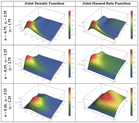
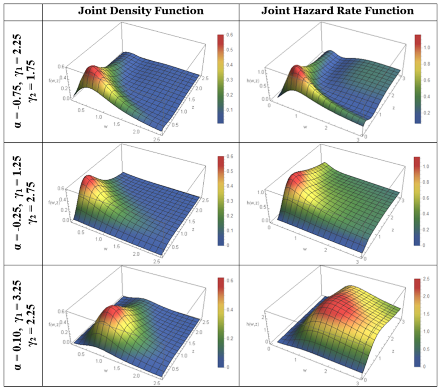
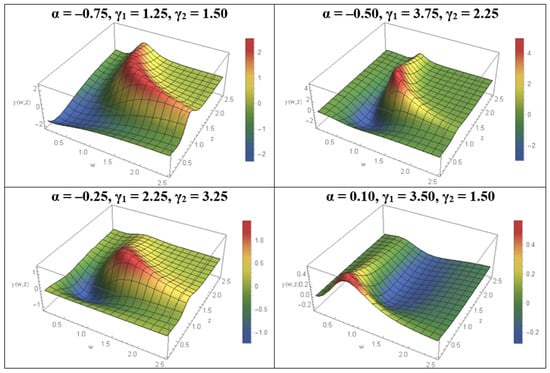
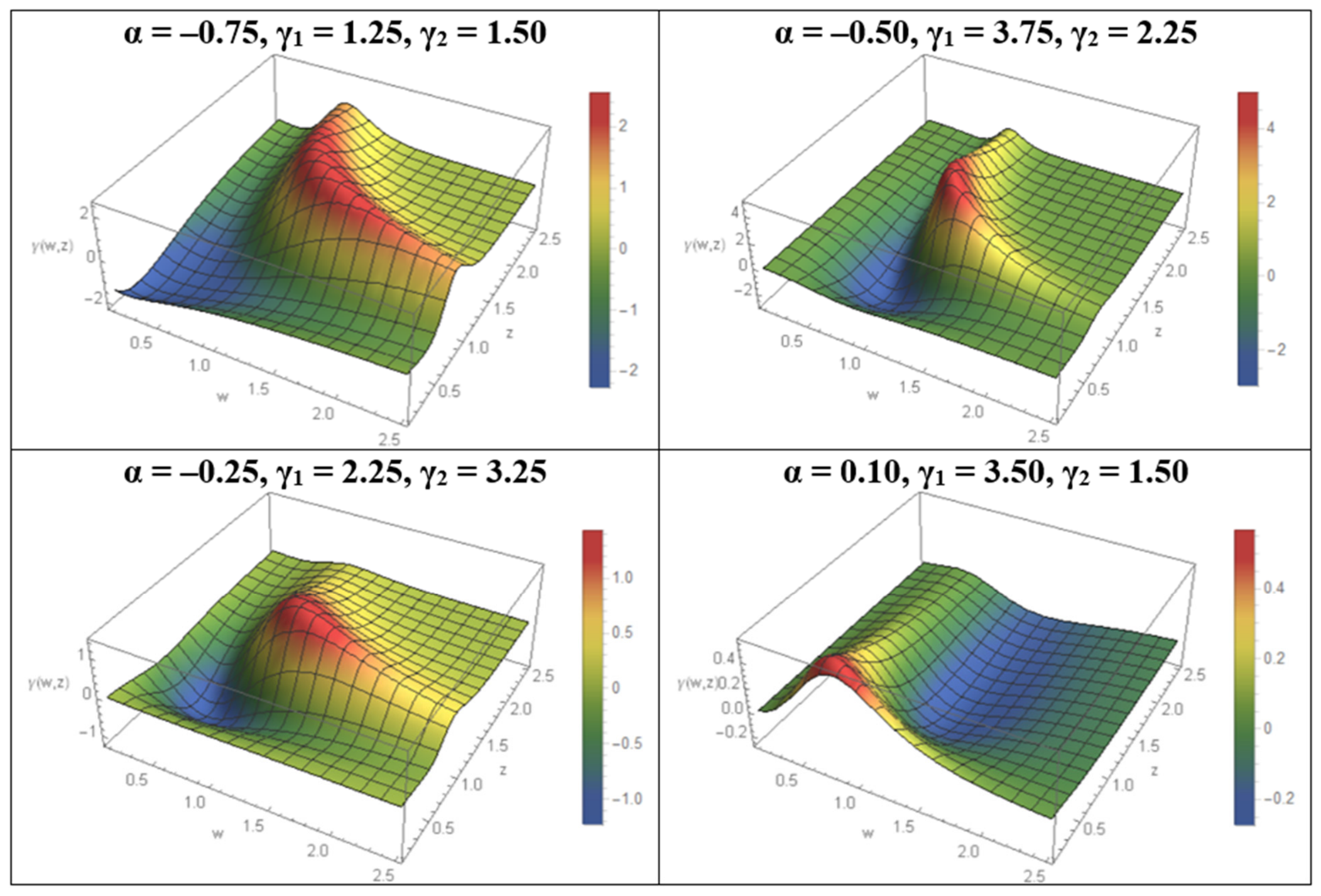
The joint reliability and hazard rate functions can be computed for specific values of the parameters. Some plots of the joint density and joint hazard rate functions are given in Figure 1 below. From the plots, we can see that when α is negative, then the hazard rate first increases and then decreases but never exceeds 1. Also, when α is positive, then the hazard rate function increases with an increase in the values of W and Z.

Figure 1. Joint density and joint hazard rate functions for DBLL distribution.

5.2. Stress-Strength Reliability Coefficient for DBLL Distribution

The stress-strength reliability coefficient for DBLL distribution is useful in its engineering applications. The stress-strength reliability coefficient for DBFDs is given in (16). The stress-strength reliability coefficient for the DBLL distribution is obtained by using the cdf of the log-logistic distribution with suitable parameters in (16) and is

$$\begin{array}{c}{R}_{DBLL}={\displaystyle {\int }_0^{\infty }\frac{{\lambda }_1^{{\gamma }_1}{\gamma }_1{w}^{{\gamma }_1+{\gamma }_2-1}}{{\left({\lambda }_1^{{\gamma }_1}+w^{{\gamma }_1}\right)}^2\left({\lambda }_2^{{\gamma }_2}+w^{{\gamma }_2}\right)}\left[1-\alpha +6\alpha w^{{\gamma }_1+{\gamma }_2}{\left({\lambda }_1^{{\gamma }_1}+w^{{\gamma }_1}\right)}^{-1}{\left({\lambda }_2^{{\gamma }_2}+w^{{\gamma }_2}\right)}^{-1}\right.}\\ \times \left.\left\{1-w^{{\gamma }_1+{\gamma }_2}{\left({\lambda }_1^{{\gamma }_1}+w^{{\gamma }_1}\right)}^{-1}{\left({\lambda }_2^{{\gamma }_2}+w^{{\gamma }_2}\right)}^{-1}\right\}\right]\mathrm{d}w.\end{array}$$

(26)

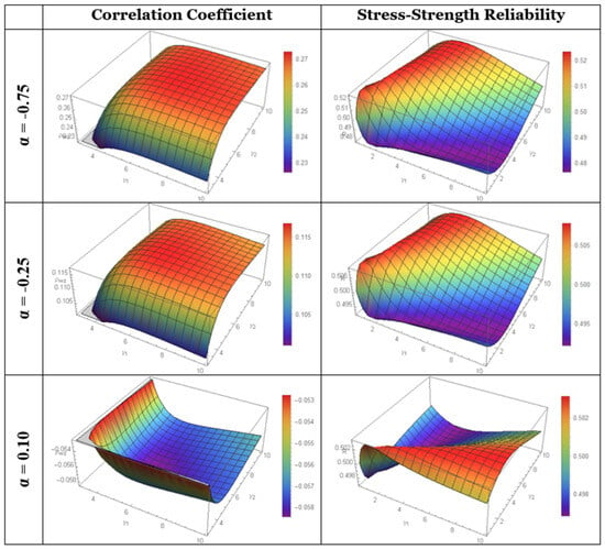
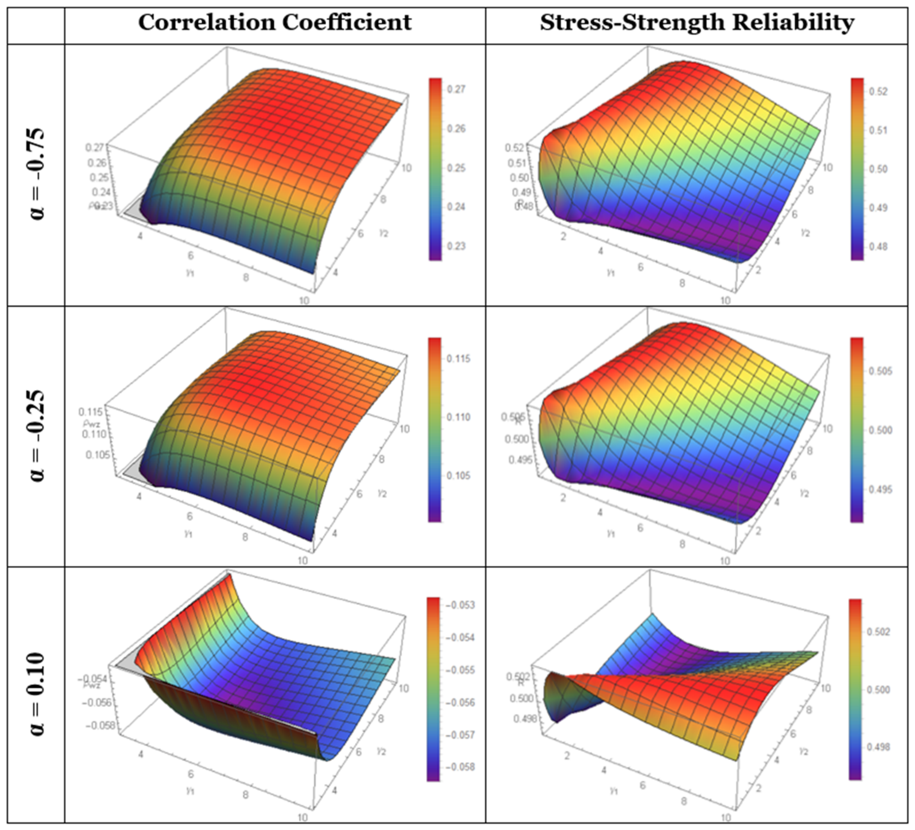
The stress-strength reliability coefficient, (26), can be computed for specific values of the parameters. It is to be noted that for λ₁ = λ₂ and γ₁ = γ₂ the integral in (26) is ½, as it should be. Some plots of the reliability coefficient are given in Figure 2 below. From these plots, we can see that the reliability revolves around 0.5. We can also see that, for α < 0 and for fixed γ₁, the stress-strength reliability coefficient decreases with an increase in γ₂. Also, when α < 0 and for fixed γ₂, the stress-strength reliability coefficient increases with an increase in γ₁.

Figure 2. Correlation and stress-strength reliability coefficients for DBLL distribution.

5.3. Joint and Conditional Moments of DBLL Distribution

The joint moments of the DBLL distribution can be readily obtained by using (11) and the moments of the log-logistic distribution. We know that the kth moment of a random variable Y having a log-logistic distribution and the kth moment of its maximum for samples of sizes 2 and 3 are

$$E\left(Y^p\right)={\displaystyle \frac{p\pi {\lambda }^p}{\gamma \mathrm{Sin}\left(p\pi /\gamma \right)}};E\left(Y_{2:2}^p\right)={\displaystyle \frac{\gamma +p}{{\gamma }^2}}{\displaystyle \frac{p\pi {\lambda }^p}{\mathrm{Sin}\left(p\pi /\gamma \right)}};E\left(Y_{3:3}^p\right)={\displaystyle \frac{\left(\gamma +p\right)\left(2\gamma +p\right)}{2{\gamma }^3}}{\displaystyle \frac{p\pi {\lambda }^p}{\mathrm{Sin}\left(p\pi /\gamma \right)}.}$$

Now, using the above expressions for pth and qth moments of W and Z in (11), the (p,q)th joint moment for the DBLL distribution is

$${\mu }_{W,Z}^{p,q}={\displaystyle \frac{pq{\pi }^2{\lambda }_1^p{\lambda }_2^q}{{\gamma }_1{\gamma }_2\mathrm{Sin}\left(p\pi /{\gamma }_1\right)\mathrm{Sin}\left(q\pi /{\gamma }_2\right)}}\left[\left(1-\alpha \right)+{\displaystyle \frac{\alpha \left({\gamma }_1+p\right)\left({\gamma }_2+q\right)}{{\gamma }_1{\gamma }_2}}\left\{3-{\displaystyle \frac{\left(2{\gamma }_1+p\right)\left(2{\gamma }_2+q\right)}{2{\gamma }_1{\gamma }_2}}\right\}\right].$$

(27)

The marginal moments of W and Z are

$${\mu }_W^p={\displaystyle \frac{p\pi {\lambda }_1^p}{{\gamma }_1\mathrm{Sin}\left(p\pi /{\gamma }_1\right)}}\left[\left(1-\alpha \right)+{\displaystyle \frac{\alpha \left({\gamma }_1+p\right)}{{\gamma }_1}}\left(3-{\displaystyle \frac{2{\gamma }_1+p}{{\gamma }_1}}\right)\right]={\displaystyle \frac{p\pi {\lambda }_1^p\left({\gamma }_1^2-\alpha p^2\right)}{{\gamma }_1^3\mathrm{Sin}\left(p\pi /{\gamma }_1\right)}} ; {\gamma }_1>p,$$

and

$${\mu }_Z^q={\displaystyle \frac{q\pi {\lambda }_2^q}{{\gamma }_2\mathrm{Sin}\left(q\pi /{\gamma }_2\right)}}\left[\left(1-\alpha \right)+{\displaystyle \frac{\alpha \left({\gamma }_2+q\right)}{{\gamma }_2}}\left(3-{\displaystyle \frac{2{\gamma }_2+q}{{\gamma }_2}}\right)\right]={\displaystyle \frac{q\pi {\lambda }_2^q\left({\gamma }_2^2-\alpha q^2\right)}{{\gamma }_2^3\mathrm{Sin}\left(q\pi /{\gamma }_2\right)}} ; {\gamma }_2>q.$$

The joint and marginal moments can be used to obtain the means, variances, and correlation coefficients between W and Z for different values of the parameters. Some plots of the correlation coefficient for λ₁ = λ₂ = 1 and for different values of α, γ₁, and γ₂ are given in Figure 2 below. The plots show that the correlation coefficient increases with an increase in γ₁ and γ₂ when α is negative and decreases with an increase in γ₁ and γ₂ when α is positive.

The pth conditional moment of W given Z = z and the qth conditional moment of Z given W = w for the DBLL distribution can be obtained by using the conditional moments of DBFDs given in (12) and (13) and are

$${\mu }_{W|z}^p={\displaystyle \frac{1}{{\phi }_{2\left(LL\right)}\left(z\right)}}{\displaystyle \frac{p\pi {\lambda }_1^p}{{\gamma }_1\mathrm{Sin}\left(p\pi /{\gamma }_1\right)}}\left[\left(1-\alpha \right)+{\displaystyle \frac{6\alpha \left({\gamma }_1+p\right)z^{{\gamma }_2}}{{\gamma }_1^2\left({\lambda }_2^{{\gamma }_2}+z^{{\gamma }_2}\right)}}\left\{1-{\displaystyle \frac{\left(2{\gamma }_1+p\right)z^{{\gamma }_2}}{2{\gamma }_1\left({\lambda }_2^{{\gamma }_2}+z^{{\gamma }_2}\right)}}\right\}\right],$$

and

$${\mu }_{Z|w}^q={\displaystyle \frac{1}{{\phi }_{1\left(LL\right)}\left(w\right)}}{\displaystyle \frac{q\pi {\lambda }_2^q}{{\gamma }_2\mathrm{Sin}\left(p\pi /{\gamma }_2\right)}}\left[\left(1-\alpha \right)+{\displaystyle \frac{6\alpha \left({\gamma }_2+q\right)w^{{\gamma }_1}}{{\gamma }_2^2\left({\lambda }_1^{{\gamma }_1}+w^{{\gamma }_1}\right)}}\left\{1-{\displaystyle \frac{\left(2{\gamma }_2+q\right)w^{{\gamma }_1}}{2{\gamma }_2\left({\lambda }_1^{{\gamma }_1}+w^{{\gamma }_1}\right)}}\right\}\right].$$

The conditional moments can be used to obtain the conditional means and variances for different values of the parameters.

5.4. A Measure of Local Dependence for DBLL Distribution

A measure of local dependence depends upon the underlying baseline distribution. The expression for this measure for DBFDs is given in (16). Now, using the pdfs and cdfs of the log-logistic distribution, a local dependence measure for the DBLL distribution is

$${\gamma }_{DBLL}\left(w,z\right)=12\alpha {\displaystyle \frac{{\lambda }_1^{{\gamma }_1}{\gamma }_1{w}^{{\gamma }_1-1}}{{\left({\lambda }_1^{{\gamma }_1}+w^{{\gamma }_1}\right)}^2}}{\displaystyle \frac{{\lambda }_2^{{\gamma }_2}{\gamma }_2{z}^{{\gamma }_2-1}}{{\left({\lambda }_2^{{\gamma }_2}+z^{{\gamma }_2}\right)}^2}}{\displaystyle \frac{{\Delta }_{3\left(LL\right)}\left(w,z\right)}{{\Delta }_{1\left(LL\right)}^2\left(w,z\right)}},$$

where

$${\Delta }_{3\left(LL\right)}\left(w,z\right)=\left[1-\alpha -{\displaystyle \frac{6w^{{\gamma }_1}{z}^{{\gamma }_2}}{\left({\lambda }_1^{{\gamma }_1}+w^{{\gamma }_1}\right)\left({\lambda }_2^{{\gamma }_2}+z^{{\gamma }_2}\right)}}\left\{1-\alpha +{\displaystyle \frac{3w^{{\gamma }_1}{z}^{{\gamma }_2}}{\left({\lambda }_1^{{\gamma }_1}+w^{{\gamma }_1}\right)\left({\lambda }_2^{{\gamma }_2}+z^{{\gamma }_2}\right)}}\right\}\right].$$

Some plots of the local dependence measure for the DBLL distribution when λ₁ = λ₂ = 1 are given in Figure 3 below.

Figure 3. Measure of local dependence for DBLL distribution.

The above plots show that, for α < 0, the local dependence measure first decreases, then increases, and then decreases with an increase in W and Z. Also, when α > 0, the local dependence measure shows the opposite behavior. Also, when α ≤ −0.5, the value of the local dependence measure may increase 1.

5.5. Parameter Estimation and Simulation for DBLL Distribution

The application of any probability distribution requires estimates of its unknown parameters. In the following, we have discussed the maximum likelihood estimation of parameters of the DBLL distribution. For this, suppose a sample of n bivariate observations is available from the DBLL distribution; then the log-likelihood function is

$$\begin{array}{cc}\hfill \mathcal{l}\left(\theta ;x,y\right)& =n{\gamma }_1\ln {\lambda }_1+n\ln {\gamma }_1+\left({\gamma }_1-1\right){\displaystyle {\sum }_{i=1}^n\ln w_i}-2{\displaystyle {\sum }_{i=1}^n\ln \left({\lambda }_1^{{\gamma }_1}+w_i^{{\gamma }_1}\right)}+n{\gamma }_2\ln {\lambda }_2+n\ln {\gamma }_2\hfill \\ & +\left({\gamma }_2-1\right){\displaystyle {\sum }_{i=1}^n\ln z_i}-2{\displaystyle {\sum }_{i=1}^n\ln \left({\lambda }_2^{{\gamma }_2}+z_i^{{\gamma }_2}\right)}+{\displaystyle {\sum }_{i=1}^n\ln \left[1-\alpha +12\alpha w_i^{{\gamma }_1}{z}_i^{{\gamma }_2}\right.}\hfill \\ & \left.\times {\left({\lambda }_1^{{\gamma }_1}+w_i^{{\gamma }_1}\right)}^{-1}{\left({\lambda }_2^{{\gamma }_2}+z_i^{{\gamma }_2}\right)}^{-1}-18\alpha w_i^{2{\gamma }_1}{z}_i^{2{\gamma }_2}{\left({\lambda }_1^{{\gamma }_1}+w_i^{{\gamma }_1}\right)}^{-2}{\left({\lambda }_2^{{\gamma }_2}+z_i^{{\gamma }_2}\right)}^{-2}\right],\hfill \end{array}$$

or

$$\begin{array}{cc}\hfill \mathcal{l}\left(\theta ;x,y\right)& =n{\gamma }_1\ln {\lambda }_1+n\ln {\gamma }_1+\left({\gamma }_1-1\right){\displaystyle {\sum }_{i=1}^n\ln w_i}-2{\displaystyle {\sum }_{i=1}^n\ln \left({\lambda }_1^{{\gamma }_1}+w_i^{{\gamma }_1}\right)}+n{\gamma }_2\ln {\lambda }_2+n\ln {\gamma }_2\hfill \\ & +\left({\gamma }_2-1\right){\displaystyle {\sum }_{i=1}^n\ln z_i}-2{\displaystyle {\sum }_{i=1}^n\ln \left({\lambda }_2^{{\gamma }_2}+z_i^{{\gamma }_2}\right)}+{\displaystyle {\sum }_{i=1}^n\ln {\Delta }_{1\left(LL\right)}\left(w_i,z_i;\theta \right)},\hfill \end{array}$$

(28)

where $\theta =\left(\alpha ,{\lambda }_1,{\lambda }_2,{\gamma }_1,{\gamma }_2\right)$, ${\Delta }_{1\left(LL\right)}\left(w_i,z_i;\theta \right)=\left[1-\alpha +12\alpha {\phi }_{1\left(LL\right)}\left(w_i,z_i\right)-18\alpha {\phi }_{2\left(LL\right)}\left(w_i,z_i\right)\right]$, ${\phi }_{1\left(LL\right)}\left(x_i,y_i\right)=w_i^{{\gamma }_1}{z}_i^{{\gamma }_2}{\left({\lambda }_1^{{\gamma }_1}+w_i^{{\gamma }_1}\right)}^{-1}{\left({\lambda }_2^{{\gamma }_2}+z_i^{{\gamma }_2}\right)}^{-1}$ and ${\phi }_{2\left(LL\right)}\left(x_i,y_i\right)=w_i^{2{\gamma }_1}{z}_i^{2{\gamma }_2}{\left({\lambda }_1^{{\gamma }_1}+w_i^{{\gamma }_1}\right)}^{-2}{\left({\lambda }_2^{{\gamma }_2}+z_i^{{\gamma }_2}\right)}^{-2}$.

The derivatives of the log-likelihood function (28) with respect to the unknown parameters are

$$U_{\alpha }={\displaystyle \frac{\partial }{\partial \alpha }}\mathcal{l}\left(\theta ;w,z\right)=-{\displaystyle \sum _{i=1}^n\frac{1-12{\phi }_{1\left(LL\right)}\left(w_i,z_i\right)+18{\phi }_{2\left(LL\right)}\left(w_i,z_i\right)}{{\Delta }_{1\left(LL\right)}\left(w_i,z_i;\theta \right)},}$$

(29)

$$U_{{\lambda }_1}={\displaystyle \frac{\partial }{\partial {\lambda }_1}}\mathcal{l}\left(\theta ;w,z\right)={\displaystyle \frac{{\gamma }_1}{{\lambda }_1}}{\displaystyle {\displaystyle \sum _{i=1}^n}\frac{w_i^{{\gamma }_1}-{\lambda }_1^{{\gamma }_1}}{w_i^{{\gamma }_1}+{\lambda }_1^{{\gamma }_1}}}+{\displaystyle {\displaystyle \sum _{i=1}^n}\frac{{\phi }_{1\left(LL\right)}\left(w_i,z_i\right)\left\{1-3{\phi }_{1\left(LL\right)}\left(w_i,z_i\right)\right\}}{{\Delta }_{1\left(LL\right)}\left(w_i,z_i;\theta \right)}\left(\frac{12\alpha {\gamma }_1{\lambda }_1^{{\gamma }_1-1}}{{\lambda }_1^{{\gamma }_1}+w_i^{{\gamma }_1}}\right),}$$

(30)

$$U_{{\lambda }_2}={\displaystyle \frac{\partial }{\partial {\lambda }_2}}\mathcal{l}\left(\theta ;w,z\right)={\displaystyle \frac{{\gamma }_2}{{\lambda }_2}}{\displaystyle {\displaystyle \sum _{i=1}^n}\frac{z_i^{{\gamma }_2}-{\lambda }_2^{{\gamma }_2}}{z_i^{{\gamma }_2}+{\lambda }_2^{{\gamma }_2}}}+{\displaystyle {\displaystyle \sum _{i=1}^n}\frac{{\phi }_{1\left(LL\right)}\left(w_i,z_i\right)\left\{1-3{\phi }_{1\left(LL\right)}\left(w_i,z_i\right)\right\}}{{\Delta }_{1\left(LL\right)}\left(w_i,z_i;\theta \right)}\left(\frac{12\alpha {\gamma }_2{\lambda }_2^{{\gamma }_2-1}{\beta }_2}{{\lambda }_2^{{\gamma }_2}+z_i^{{\gamma }_2}}\right),}$$

(31)

$$\begin{array}{c}{U}_{{\gamma }_1}={\displaystyle \frac{\partial }{\partial {\gamma }_1}}\mathcal{l}\left(\theta ;w,z\right)={\displaystyle \frac{n}{{\gamma }_1}}-{\displaystyle {\sum }_{i=1}^n\ln \left(w_i/{\lambda }_1\right)}+2{\displaystyle {\displaystyle \sum _{i=1}^n}\frac{{\lambda }_1^{{\gamma }_1}\ln \left(w_i/{\lambda }_1\right)}{{\lambda }_1^{{\gamma }_1}+w_i^{{\gamma }_1}}}\\ +12\alpha {\displaystyle \sum _{i=1}^n\frac{{\phi }_{1\left(LL\right)}\left(w_i,z_i\right)\left\{1-3{\phi }_{1\left(LL\right)}\left(w_i,z_i\right)\right\}}{{\Delta }_{1\left(LL\right)}\left(w_i,z_i;\theta \right)}\left\{\frac{{\lambda }_1^{{\gamma }_1}\ln \left(w_i/{\lambda }_1\right)}{{\lambda }_1^{{\gamma }_1}+w_i^{{\gamma }_1}}\right\},}\end{array}$$

(32)

and

$$\begin{array}{c}{U}_{{\gamma }_2}={\displaystyle \frac{\partial }{\partial {\gamma }_2}}\mathcal{l}\left(\theta ;w,z\right)={\displaystyle \frac{n}{{\gamma }_2}}-{\displaystyle {\sum }_{i=1}^n\ln \left(z_i/{\gamma }_2\right)}+2{\displaystyle {\displaystyle \sum _{i=1}^n}\frac{{\lambda }_2^{{\gamma }_2}\ln \left(z_i/{\gamma }_2\right)}{{\lambda }_2^{{\gamma }_2}+z_i^{{\gamma }_2}}}\\ +12\alpha {\displaystyle \sum _{i=1}^n\frac{{\phi }_{1\left(LL\right)}\left(w_i,z_i\right)\left\{1-3{\phi }_{1\left(LL\right)}\left(w_i,z_i\right)\right\}}{{\Delta }_{1\left(LL\right)}\left(w_i,z_i;\theta \right)}\left\{\frac{{\lambda }_2^{{\gamma }_2}\ln \left(z_i/{\gamma }_2\right)}{{\lambda }_2^{{\gamma }_2}+z_i^{{\gamma }_2}}\right\}.}\end{array}$$

(33)

The maximum likelihood estimators of the parameters can be obtained by equating the score functions, (29)–(33), to zero and solving the resulting non-linear equations. The maximum likelihood estimators are asymptotically normally distributed with mean vector equal to the true parameters and the covariance matrix $I_{DBLL}^{-1}\left(\theta \right)$, where $I_{DBLL}\left(\theta \right)$ is the Fisher information matrix.

We have conducted extensive simulations to see the performance of maximum likelihood estimation. The algorithm for the simulation is given below.

• Generate random samples of sizes 20, 50, 100, 200, and 500 from the DBLL distribution by using some prespecified values of the parameters α, λ₁, λ₂, γ₁, and γ₂ and using the conditional distribution approach as given in (17) and (18).
• Compute the MLEs of the parameters by using the sample obtained in Step-1.
• Repeat Step-1 and Step-2 for 50,000 time.
• Compute the average, standard error, and root mean square error of estimates by using

$${\widehat{\theta }}_k=N^{-1}{\displaystyle {\sum }_{j=1}^N{\widehat{\theta }}_{kj}},SE\left({\widehat{\theta }}_k\right)=\sqrt{N^{-1}{\displaystyle {\sum }_{j=1}^N{\left({\widehat{\theta }}_{kj}-{\widehat{\theta }}_k\right)}^2}},RMSE\left({\widehat{\theta }}_k\right)=\sqrt{N^{-1}{\displaystyle {\sum }_{j=1}^N{\left({\widehat{\theta }}_{kj}-{\theta }_k\right)}^2}},$$

where ${\widehat{\theta }}_{kj}$ is the maximum likelihood estimate of the kth element of $\theta =\left(\alpha ,{\lambda }_1,{\lambda }_2,{\gamma }_1,{\gamma }_2\right)$ obtained from the jth simulation and ${\theta }_k$ is the pre-sepecified value of the parameter.

Also, the pre-specified values of the parameters are used as the starting values for the simulation. The simulation results are given in Table 1 below. The table also contains information about the coverage rate for a 95% interval at each sample size, where the coverage rate is computed as the proportion of time the estimated value of the parameter is within ${\widehat{\theta }}_k\pm 1.96\times SE\left({\widehat{\theta }}_k\right)$.

Table 1. Simulation results for BDLL distribution.

n		α = –0.25	λ1 = 2.25	λ2 = 1.75	γ1 = 3.50	γ2 = 2.75
20	Estimate	−0.25006	2.25042	1.75002	3.50019	2.75001
	SE	0.07205	0.16680	0.16640	0.11864	0.18176
	RMSE	0.07195	0.16690	0.16600	0.11844	0.18126
	Cov. Rate	0.93990	0.92230	0.92136	0.94825	0.96542
50	Estimate	−0.25029	2.24962	1.75041	3.50028	2.75014
	SE	0.07190	0.14584	0.11520	0.16400	0.15376
	RMSE	0.07210	0.14554	0.11550	0.16360	0.15416
	Cov. Rate	0.95059	0.95150	0.92546	0.92556	0.93547
100	Estimate	−0.25049	2.24997	1.74998	3.49991	2.75013
	SE	0.07185	0.12328	0.10312	0.10608	0.14272
	RMSE	0.07215	0.12288	0.10292	0.10638	0.14222
	Cov. Rate	0.92984	0.95847	0.93761	0.92790	0.96794
200	Estimate	−0.24955	2.25007	1.75009	3.50010	2.74998
	SE	0.07300	0.09761	0.10016	0.09682	0.12544
	RMSE	0.07310	0.09711	0.09996	0.09652	0.12534
	Cov. Rate	0.93203	0.94085	0.92626	0.93820	0.93509
500	Estimate	−0.25030	2.25000	1.75003	3.50025	2.75013
	SE	0.07210	0.07864	0.10840	0.08992	0.11772
	RMSE	0.07160	0.07854	0.10870	0.09022	0.11782
	Cov. Rate	0.94836	0.96027	0.94222	0.94998	0.95361
n		α = 0.12	λ1 = 1.75	λ2 = 3.25	γ1 = 2.25	γ2 = 3.75
20	Estimate	0.11997	1.74965	3.24961	2.25028	3.7498
	SE	0.06930	0.22571	0.21207	0.16771	0.28838
	RMSE	0.06890	0.22561	0.21247	0.16761	0.28888
	Cov. Rate	0.94667	0.95846	0.92667	0.93685	0.95305
50	Estimate	0.12007	1.75005	3.24984	2.25041	3.74987
	SE	0.05891	0.26540	0.19191	0.15134	0.19685
	RMSE	0.05871	0.26410	0.19321	0.15034	0.19735
	Cov. Rate	0.93210	0.93927	0.94425	0.93376	0.92063
100	Estimate	0.12011	1.74998	3.25019	2.24995	3.75001
	SE	0.05841	0.22172	0.18708	0.12442	0.17414
	RMSE	0.05831	0.22152	0.18688	0.12402	0.17414
	Cov. Rate	0.95896	0.94161	0.92034	0.92659	0.96694
200	Estimate	0.11993	1.74993	3.2497	2.24982	3.75032
	SE	0.04982	0.18111	0.16542	0.10727	0.13761
	RMSE	0.04992	0.18081	0.16532	0.10687	0.13791
	Cov. Rate	0.94122	0.93619	0.92617	0.94481	0.96047
500	Estimate	0.12011	1.74975	3.25015	2.24974	3.74986
	SE	0.04941	0.15351	0.13452	0.10426	0.11947
	RMSE	0.04891	0.15361	0.13462	0.10406	0.11997
	Cov. Rate	0.93445	0.95066	0.94179	0.96226	0.96196

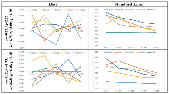
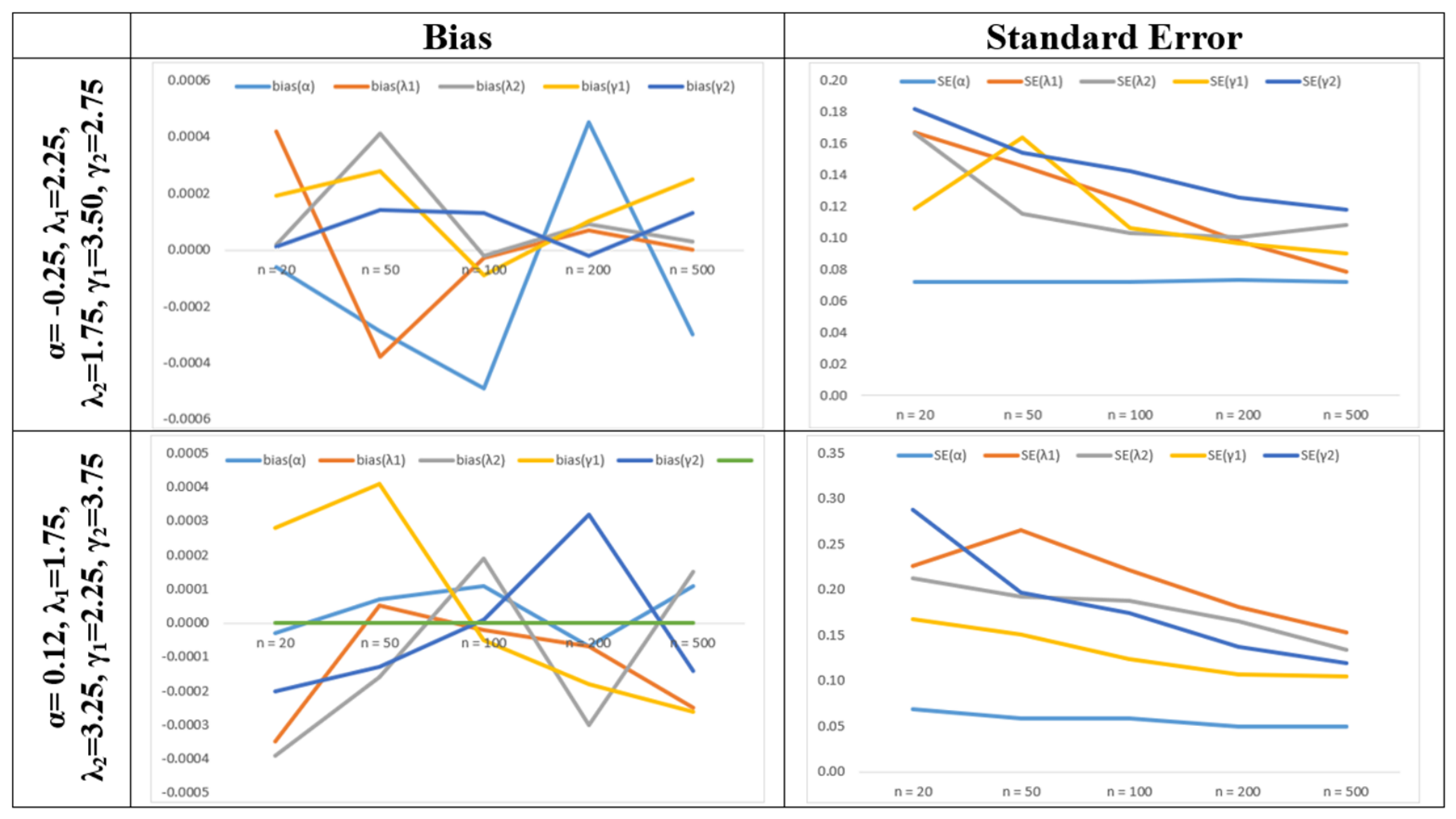
The simulation results show that the estimates are consistent as the standard error of estimates decreases with an increase in the sample size. The plots of bias and standard error of estimates are given in Figure 4 below. The figures also confirm the simulation results.

Figure 4. Bias and standard error of estimates.

We will now apply the DBLL distribution to model the Saudi commercial bank LCs. This application is given below.

6. Modeling Price Index of Saudi Commodities

In the following, we have used the proposed DBLL distribution to model the PI of Saudi commodities. We have used the price index of various Saudi commodities for this purpose. We have used two data sets for this purpose. The data have been obtained from the Saudi Arabian Central Bank’s website (www.sama.gov.sa (accessed on 25 July 2026)). The description of the data is given in Table 2 below.

Table 2. Description of the variables used for the study.

Data 1 n = 136	W	Price Index of Various Commodities for January 2015
	Z	Price Index of Various Commodities for January 2020
Data 2 n = 136	W	Price Index of Various Commodities for July 2015
	Z	Price Index of Various Commodities for July 2020

The data are essentially cross-sectional and the observations are independent.

Some useful summary measures of two data sets are given in Table 3 below.

Table 3. Summary measures for two data sets.

Statistics	Data 1		Data 2
	W	Z	W	Z
Minimum	4.5053	3.9703	4.3399	3.7865
Mean	4.6056	4.6386	4.6071	4.7288
Q1	4.6032	4.5401	4.5951	4.6265
Median	4.6052	4.5981	4.6052	4.7065
Q3	4.6072	4.6950	4.6141	4.8097
Maximum	4.9793	5.8159	4.7596	5.6522
Variance	0.0003	0.0657	0.0019	0.0648
Skewness	−0.9393	2.0544	−1.3378	0.8934
Correlation	0.0479		0.2102

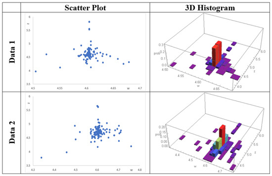
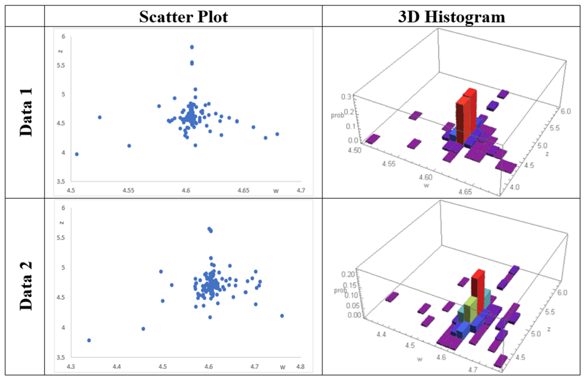
The scatter plots and joint histograms of the two data sets are given in Figure 5 below.

Figure 5. Scatter plots and histograms of two data sets.

The summary measures indicate that there is a low correlation between the variables, which is also visible from the scatter plots. We have fitted the following bivariate distributions, alongside the DBLL distribution, to model the two data sets:

Gumbel Bivariate Log-logistic (GBLL) Distribution (obtained by using the log-logistic distribution as a baseline distribution in the Gumbel [1] bivariate family of distributions)

$$f_{GBLL}\left(w,z\right)={\displaystyle \frac{{\lambda }_1^{{\gamma }_1}{\lambda }_2^{{\gamma }_2}{\gamma }_1{\gamma }_2{w}^{{\gamma }_1-1}{z}^{{\gamma }_2-1}}{{\left({\lambda }_1^{{\gamma }_1}+w^{{\gamma }_1}\right)}^2{\left({\lambda }_2^{{\gamma }_2}+z^{{\gamma }_2}\right)}^2}}\left[1+\alpha \left({\displaystyle \frac{{\lambda }_1^{{\gamma }_1}-w^{{\gamma }_1}}{{\lambda }_1^{{\gamma }_1}+w^{{\gamma }_1}}}\right)\left({\displaystyle \frac{{\lambda }_2^{{\gamma }_2}-z^{{\gamma }_2}}{{\lambda }_2^{{\gamma }_2}+z^{{\gamma }_2}}}\right)\right].$$

Huang and Kotz Bivariate Log-logistic (HKBLL) Distribution (obtained by using the log-logistic distribution as a baseline distribution in the Huang and Kotz [4] bivariate family of distributions)

$$f_{HKBLL}\left(w,z\right)={\displaystyle \frac{{\lambda }_1^{{\gamma }_1}{\lambda }_2^{{\gamma }_2}{\gamma }_1{\gamma }_2{w}^{{\gamma }_1-1}{z}^{{\gamma }_2-1}}{{\left({\lambda }_1^{{\gamma }_1}+w^{{\gamma }_1}\right)}^2{\left({\lambda }_2^{{\gamma }_2}+z^{{\gamma }_2}\right)}^2}}\left[1+\alpha \left\{1-{\displaystyle \frac{\beta w^{\left(\beta -1\right){\gamma }_1}}{{\left({\lambda }_1^{{\gamma }_1}+w^{{\gamma }_1}\right)}^{\beta -1}}}\right\}\left\{1-{\displaystyle \frac{\beta z^{\left(\beta -1\right){\gamma }_2}}{{\left({\lambda }_2^{{\gamma }_2}+z^{{\gamma }_2}\right)}^{\beta -1}}}\right\}\right].$$

Darwish-Shahbaz-Shahbaz Bivariate Log-logistic (DSSBLL) Distribution (obtained by using the log-logistic distribution as a baseline distribution in the Darwish et al. [10] bivariate family of distributions)

$$f_{DSSBLL}\left(w,z\right)={\displaystyle \frac{{\lambda }_1^{{\gamma }_1}{\lambda }_2^{{\gamma }_2}{\gamma }_1{\gamma }_2{w}^{{\gamma }_1-1}{z}^{{\gamma }_2-1}}{{\left({\lambda }_1^{{\gamma }_1}+w^{{\gamma }_1}\right)}^2{\left({\lambda }_2^{{\gamma }_2}+z^{{\gamma }_2}\right)}^2}}\left[1+\alpha -\alpha \beta \delta {\displaystyle \frac{w^{\left(\beta -1\right){\gamma }_1}}{{\left({\lambda }_1^{{\gamma }_1}+w^{{\gamma }_1}\right)}^{\beta -1}}}{\displaystyle \frac{z^{\left(\delta -1\right){\gamma }_2}}{{\left({\lambda }_2^{{\gamma }_2}+z^{{\gamma }_2}\right)}^{\delta -1}}}\right].$$

Kimeldorf and Sampson Bivariate Log-logistic (KSBLL) Distribution (obtained by using the log-logistic distribution as a baseline distribution in the Kimeldorf and Sampson [3] bivariate family of distributions)

$$f_{KSBLL}\left(x,y\right)={\displaystyle \frac{{\lambda }_1^{{\gamma }_1}{\lambda }_2^{{\gamma }_2}{\gamma }_1{\gamma }_2{w}^{{\gamma }_1-1}{z}^{{\gamma }_2-1}}{{\left({\lambda }_1^{{\gamma }_1}+w^{{\gamma }_1}\right)}^2{\left({\lambda }_2^{{\gamma }_2}+z^{{\gamma }_2}\right)}^2}}{\Delta }_{KS\left(LL\right)},$$

where

$${\Delta }_{KS\left(LL\right)}=1+\alpha \left({\displaystyle \frac{{\lambda }_1^{{\gamma }_1}-w^{{\gamma }_1}}{{\lambda }_1^{{\gamma }_1}+w^{{\gamma }_1}}}\right)\left({\displaystyle \frac{{\lambda }_2^{{\gamma }_2}-z^{{\gamma }_2}}{{\lambda }_2^{{\gamma }_2}+z^{{\gamma }_2}}}\right)+\beta \left\{1-3{\left({\displaystyle \frac{w^{{\gamma }_1}}{{\lambda }_1^{{\gamma }_1}+w^{{\gamma }_1}}}\right)}^2\right\}\left\{1-3\left({\displaystyle \frac{z^{{\gamma }_2}}{{\lambda }_2^{{\gamma }_2}+z^{{\gamma }_2}}}\right)\right\}.$$

The maximum likelihood estimates for various distributions are given in Table 4 below.

Table 4. Maximum likelihood estimates of parameters.

Distribution	Parameter	Data 1		Data 2
		Estimate	SE	Estimate	SE
DBLL	α	−0.4012	0.0123	−0.1981	0.0528
	λ1	4.9519	0.0578	4.6092	0.5033
	λ2	4.7197	0.0171	6.1305	1.7978
	γ1	9.3111	0.8842	9.0811	2.0647
	γ2	8.4625	0.7801	0.6624	0.0271
GBLL	α	−0.3406	0.4765	−0.4037	0.1152
	λ1	4.6094	0.0149	4.6101	0.8596
	λ2	4.6051	0.0105	3.8508	0.5914
	γ1	9.1811	1.3614	5.9876	0.7195
	γ2	7.0058	1.5137	0.8501	0.2218
HKBLL	α	0.4997	0.1852	−0.4998	0.0647
	β	3.9808	1.6341	3.4965	0.4157
	λ1	6.4894	1.1542	4.2597	0.0338
	λ2	5.1424	0.1347	5.6574	0.4912
	γ1	2.2038	0.4904	8.7780	0.7864
	γ2	3.8999	0.3329	1.3322	0.1131
DSSBLL	α	−0.4998	0.1182	−0.4787	0.0524
	β	0.9985	0.0829	1.0179	0.0866
	δ	1.1886	0.1195	1.0459	0.1042
	λ1	3.6345	0.2337	3.3621	0.2848
	λ2	3.7665	0.2282	3.7922	0.2239
	γ1	2.3410	0.2448	2.5741	0.3756
	γ2	2.2475	0.2141	2.6356	0.2783
KSBLL	α	−0.4989	0.1767	−0.3687	0.1152
	β	0.4993	0.1532	0.4969	0.1871
	λ1	5.4104	1.8524	4.6737	0.3124
	λ2	4.0441	1.0534	5.2245	0.3719
	γ1	8.2066	1.8712	4.7059	0.3964
	γ2	7.1242	1.7078	4.8554	0.3459

We have computed the Akaike information criteria (AIC), corrected AIC (AICc), and Bayesian information criteria (BIC), and we see the goodness of fit of various models. We have also used the bivariate Kolmogorov–Simirnov goodness of fit test [29] to test the significance of various distributions in fitting the data. The results of these measures are given in Table 5 below.

Table 5. Various measures of goodness of fit.

Data	Measure	Distributions
		DBLL	GBLL	HKBLL	DSBLL	KSBLL
1	Log-Like.	−115.3758	−193.0212	−493.1226	−584.1661	−292.5157
	AIC	240.7516	396.0424	998.2452	1182.3322	597.0314
	AICc	241.2096	396.5004	998.8914	1183.2004	597.6776
	BIC	255.3515	410.6423	1015.7651	1202.7721	614.5513
	KS p-value	0.3584	0.0985	0.0001	0.0001	0.0085
2	Log-Like.	−301.3734	−367.8816	−474.6114	−570.2381	−373.1733
	AIC	612.7468	745.7632	961.2228	1154.4762	758.3466
	AICc	613.2048	746.2212	961.8690	1155.3444	758.9928
	BIC	627.3467	760.3631	978.7427	1174.9161	775.8665
	KS p-value	0.2987	0.0685	<0.0001	<0.0001	0.0006

It is clear from the above table that the proposed DBLL distribution is the best fit for the two data sets as it has the smallest AIC, AICc, and BIC alongside the highest p-value of the Kolmogorov–Smirnov test. We can, therefore, conclude that the proposed DBLL distribution is the best distribution for modeling the settled import LCs of the commercial banks in Saudi Arabia.

7. Conclusions and Further Recommendations

In this paper, a new bivariate family of distributions, the Darwish bivariate family of distributions (DBFDs), is proposed that can efficiently capture the complex behavior of a complex data set. The proposed family of distributions depends upon one dependence parameter λ that has an inverse effect on the dependence measures. Some important properties of the proposed family of distributions are discussed. It is observed that the proposed family of distributions is useful for modeling the bivariate data sets that have smaller measures of interdependence. The proposed family of distributions is used to obtain a new bivariate log-logistic distribution, namely the Darwish bivariate log-logistic (DBLL) distribution. Some important properties of the DBLL distribution are discussed. It is found that the dependence parameter α of DBFDs has a significant effect on the correlation coefficient between the variables of the DBLL distribution. It is found that the correlation coefficient is positive when λ is negative and vice versa. It is also found that the stress-strength reliability coefficient for the DBLL distribution revolves around 0.5. The proposed DBLL distribution, alongside some other competing bivariate log-logistic distributions, is used to model the price index of various Saudi commodities. It is found that the proposed DBLL distribution is the most suitable distribution for modeling the price index of Saudi commodities.

As future research, the DBFDs can be used to obtain some other bivariate distributions by using some other baseline distributions. Two different baseline distributions can also be used in DBFDs to obtain more complex distributions. For example, if the random variable X in DBFDs has a Pareto distribution, and the random variable Y has a Lomax distribution, then we can get the Darwish bivariate Pareto Lomax (DBPL) distribution. Several other distributions can be generated and studied in a similar way. In a nutshell, the proposed DBFDs are a useful addition to the literature of bivariate families of distributions.

References

- Gumbel, E.J. Multivariate distributions with given marginals and analytical examples. Bull. l’Institut Int. Stat. 1960, 37, 363–373. [Google Scholar]
- Gumbel, E.J. Bivariate logistic distributions. J. Am. Stat. Assoc. 1961, 56, 335–349. [Google Scholar] [CrossRef] [Scilit]
- Kimeldorf, G.; Sampson, A. Uniform representations of bivariate distributions. Commun. Stat. 1975, 4, 617–627. [Google Scholar] [CrossRef] [Scilit]
- Huang, J.S.; Kotz, S. Modifications of the Farlie-Gumbel-Morgenstern distributions: A tough hill to climb. Matrika 1999, 49, 307–323. [Google Scholar] [CrossRef] [Scilit]
- Balakrishnan, N.; Lai, C.D. Continuous Bivariate Distributions, 2nd ed.; Springer: New York, NY, USA, 2009. [Google Scholar]
- Nelsen, R.B. An Introduction to Copulas, 2nd ed.; Springer: New York, NY, USA, 2006. [Google Scholar]
- Sarabia, J.M.; Prieto, F.; Jorda, V. Bivariate beta–generated distributions with applications to well-being data. J. Stat. Dist. Appl. 2014, 1, 15. [Google Scholar] [CrossRef] [Scilit]
- Darwish, J.A.; Al turk, L.I.; Shahbaz, M.Q. The bivariate transmuted family of distributions: Theory and applications. Comp. Syst. Sci. Eng. 2021, 36, 131–144. [Google Scholar] [CrossRef] [Scilit]
- Ganji, M.; Bevrani, H.; Golzar, N.H. A new method for generating continuous bivariate distribution families. J. Iran. Stat. Soc. 2018, 17, 109–129. [Google Scholar] [CrossRef] [Scilit]
- Darwish, J.A.; Shahbaz, S.H.; Shahbaz, M.Q. A new class of bivariate distributions: Properties, Estimation and Modeling. Mathematics 2024, 12, 4021. [Google Scholar] [CrossRef] [Scilit]
- Shahbaz, S.H.; Shahbaz, M.Q. A New Bivariate Exponentiated Family of Distributions: Properties and Applications. Pak. J. Stat. Oper. Res. 2025, 21, 137–161. [Google Scholar] [CrossRef] [Scilit]
- Alzaatreh, A.; Lee, C.; Famoye, F. A new method of generating families of continuous distributions. Metron 2013, 71, 63–79. [Google Scholar] [CrossRef] [Scilit]
- Shahbaz, M.Q.; Shahbaz, S.H.; Ahsanullah, M. Univariate Families of Distributions; CRC Press, Taylor & Francis Group: New York, NY, USA, 2026. [Google Scholar]
- Olkin, I.; Liu, R. A bivariate beta distribution. Stat. Probab. Lett. 2003, 62, 407–412. [Google Scholar] [CrossRef] [Scilit]
- Rahman, M.M.; Al–Zahrani, B.; Shahbaz, S.H.; Shahbaz, M.Q. Cubic Transmuted Uniform Distribution: An Alternative to Beta and Kumaraswamy Distribution. Eur. J. Pure Appl. Math. 2019, 12, 1106–1121. [Google Scholar] [CrossRef] [Scilit]
- David, H.A.; Nagaraja, H.N. Order Statistics; John Wiley Inc.: Hoboken, NJ, USA, 2003. [Google Scholar]
- Shahbaz, M.Q.; Ahsanullah, M.; Shahbaz, S.H.; Al-Zahrani, B. Ordered Random Variables: Theory and Applications; Atlantis Press: Dordrecht, The Netherlands; Springer: Berlin/Heidelberg, Germany, 2016. [Google Scholar]
- Moore, D.F. Applied Survival Analysis Using R; Springer: New York, NY, USA, 2016. [Google Scholar]
- Basu, A.P. Bivariate failure rate. J. Am. Stat. Assoc. 1971, 66, 103–104. [Google Scholar] [CrossRef]
- Johnson, N.L.; Kotz, S. A vector multivariate hazard rate. J. Multivar. Anal. 1987, 5, 53–66. [Google Scholar]
- Holland, P.V.; Wang, Y.J. Dependence function for continuous bivariate densities. Commun. Stat. Theory Methods 1987, 16, 863–876. [Google Scholar] [CrossRef] [Scilit]
- Fisk, P.R. The graduation of income distributions. Econometrica 1961, 29, 171–185. [Google Scholar] [CrossRef] [Scilit]
- Gupta, R.C.; Akman, O.; Lvin, S. A study of log-logistic model in survival analysis. Biom. J. 1999, 41, 431–443. [Google Scholar] [CrossRef] [Scilit]
- Aryal, G.R. Transmuted log-logistic distribution. J. Stat. Appl. Probab. 2013, 2, 11–20. [Google Scholar] [CrossRef] [Scilit]
- Ramos, M.W.A. The Zografos-Balakrishnan Log-Logistic Distribution. Properties and Application. J. Stat. Theory Appl. 2013, 12, 244–255. [Google Scholar] [CrossRef] [Scilit]
- Para, B.A.; Jan, T.R.; Subzar, M. A New Three Parameter Log-Logistic Model for Survival Data Analysis. J. Stat. Appl. Probab. 2021, 21, 705–714. [Google Scholar] [CrossRef] [Scilit]
- Rahman, M.M.; Darwish, J.A.; Shahbaz, S.H.; Hamedani, G.G.; Shahbaz, M.Q. A New Cubic Transmuted Log-Logistic Distribution: Properties, Applications and Characterizations. Adv. Appl. Stat. 2024, 91, 335–361. [Google Scholar] [CrossRef] [Scilit]
- Muse, A.H.; Mwalili, S.M.; Ngesa, O. On the log-logistic distribution and its generalizations: A survey. Int. J. Stat. Probab. 2021, 10, 93–125. [Google Scholar] [CrossRef] [Scilit]
- Justel, A.; Peña, D.; Zamar, R. A multivariate Kolmogorov-Smirnov test of goodness of fit. Stat. Probab. Lett. 1997, 35, 251–259. [Google Scholar] [CrossRef] [Scilit]
Disclaimer/Publisher’s Note: The statements, opinions and data contained in all publications are solely those of the individual author(s) and contributor(s) and not of MDPI and/or the editor(s). MDPI and/or the editor(s) disclaim responsibility for any injury to people or property resulting from any ideas, methods, instructions or products referred to in the content. |
© 2026 by the author. Licensee MDPI, Basel, Switzerland. This article is an open access article distributed under the terms and conditions of the Creative Commons Attribution (CC BY) license.