Measuring Urban Economic Performance in G7 Countries Through a Novel Grey-Based Multi-Criteria Framework

Abstract

Cities are the main sites of production, employment, and capital accumulation in advanced economies, which places urban economic performance at the centre of economic policy and urban governance. This work develops an integrated grey-based multi-criteria approach for assessing that performance and applies it to the sixteen G7 cities covered by the Global Power City Index (GPCI). Criterion weights are obtained with Grey RANCOM (G-RANCOM), which converts the ordinal rankings of a five-member expert panel into interval weights, and the cities are ranked with Grey MUNRA (G-MUNRA), which aggregates linear, vector, and non-linear normalization. Each performance entry is an interval bounded by the minimum and the maximum annual score observed in the GPCI Economy function over 2021–2025. Market size, economic vitality, and business environment emerge as the most influential criteria, and New York, London, and Tokyo occupy the highest positions, while Osaka, Milan, and Fukuoka occupy the last three. Robustness is tested via scenario analyses on the model parameters and through a global analysis of 100,000 replications in which all of them vary jointly. New York holds the first position in 74% of the replications and the three lowest positions are unchanged in 87%, whereas cities in adjacent middle positions are not separated reliably. Rankings produced by five established grey approaches, by crisp and fuzzy counterparts, and by the published GPCI Economy rankings agree with the reported ordering, with Spearman correlations between 0.92 and 1.00. The framework offers urban policymakers a transparent benchmarking tool for evidence-based competitiveness strategies.

1. Introduction

Sustainable development has become a central guiding principle for urban policy and planning in the 21st century and is commonly conceptualized around three interdependent pillars: economic, social, and environmental sustainability [1,2]. While these dimensions are mutually reinforcing, economic sustainability occupies a foundational position, as the ability to generate stable output, productive employment, and fiscal resources over time conditions the feasibility of both social welfare provision and environmental protection [3,4,5]. In urban contexts, economic sustainability is not an abstract or autonomous outcome; rather, it is fundamentally shaped by cities’ economic performance, which determines their capacity to sustain growth, absorb economic shocks, and support long-term development trajectories [6,7,8,9].

Accordingly, economic performance constitutes an indispensable prerequisite for urban sustainability [10]. Cities with strong economic performance are better positioned to generate employment, mobilize public revenues, and finance investments in infrastructure, social services, and environmental improvement [11,12,13]. By contrast, persistent weaknesses in urban economic performance constrain fiscal capacity, exacerbate social inequalities, and undermine long-term sustainability objectives. In an increasingly globalized economic environment, the most successful cities are those capable of formulating and implementing development strategies that extend beyond national economic dynamics and position them as competitive actors in international markets [14]. This research therefore focuses on comparative assessment of urban economic performance, rather than sustainability in a broad sense.

Despite the acknowledged importance of benchmarking urban economic performance, systematic evaluation poses substantial analytical challenges because urban economies are inherently multi-dimensional and heterogeneous. In response, multi-criteria decision-making (MCDM) approaches enable the simultaneous consideration of multiple, often conflicting, performance dimensions within a unified structure and make their relative importance explicit through structured weighting and aggregation procedures, thereby facilitating robust and comparable assessments of complex alternatives [15]. Despite the widespread application of MCDM techniques in economic, environmental, and sustainability-related studies, existing applications have predominantly focused on countries or regions [16,17,18,19]. City-level analyses—especially those explicitly centred on economic performance—remain comparatively limited, despite the pivotal role of cities in contemporary economic systems.

Within this context, the Global Power City Index (GPCI) provides an internationally recognized empirical foundation for evaluating cities from a multi-dimensional perspective [20]. Its Economy function comprises 13 indicators organized into six groups: market size, market attractiveness, economic vitality, human capital, business environment, and ease of doing business, which capture the core structural dimensions shaping urban economic performance. The index nevertheless remains descriptive in construction. It aggregates indicator scores without differentiating the relative importance of these six dimensions, so their contribution is fixed by construction rather than derived from a decision-analytic procedure; it also reports a single score per city and year, leaving the imprecision of the underlying measurement unexpressed. Closing both gaps requires an MCDM structure in which criterion importance is derived explicitly and imprecision is carried through the evaluation.

To address these gaps, the current study proposes an integrated grey-based MCDM approach to assess and compare cities’ economic performance. Building on the economic dimension of the GPCI, the proposed approach uses a grey-based RANCOM tool to determine criterion importance and a grey-based MUNRA tool to generate robust city rankings.

The usage of interval grey numbers in this research follows from the kind of information available at each stage of the analysis. A fuzzy model would require a membership function, and such functions are generally specified from expert intuition, which varies across decision makers and weakens methodological consistency [21,22]. A probabilistic model would require treating a city’s five annual observations as draws from a stable distribution, whereas they are successive measurements of a changing quantity. A grey number requires only a lower and an upper bound [23,24], and bounds are exactly what the two inputs of this study supply. The published GPCI scores carry no dispersion estimate, so the range observed over the 2021–2025 period is the only imprecision in the source documents. The experts, in turn, are asked for rank positions rather than degrees of preference (Section 4.2), so each pairwise relation is known only as one of three ordinal states. Such states can be bounded, but they cannot identify a membership function. Grey numbers are therefore adopted because they represent what is known about the data and the judgments without adding what is not. Section 5.5 examines whether this representation also yields better rankings.

Within this interval grey environment, the two methods serve complementary functions at the two stages of the decision process. G-RANCOM requires only a ranking of the criteria, which reduces the cognitive effort demanded of the experts and permits ties between criteria of equal importance. It is executed for each expert individually, so divergence of opinion is preserved in the width of the weight intervals rather than eliminated by a consensus ranking. G-MUNRA evaluates the alternatives under linear, vector, and non-linear normalization simultaneously and aggregates the three outcomes, which limits scale sensitivity and the risk of rank reversal. Grey models operating at both stages already exist (Section 2), but they obtain the weights either from the data alone, without consulting experts, or from experts who must state how much more important one criterion is than another, and they rank the alternatives under a single normalization scheme. RANCOM and MUNRA have not previously been formulated with interval grey numbers, and their combination carries uncertainty from the first expert judgement to the final ranking without asking the experts for more than an order.

To demonstrate the framework’s effectiveness and practical applicability, we conduct a comprehensive case study. The case study compares the economic performance of sixteen cities across G7 economies, representing some of the most influential urban centres in the global economic system.

Accordingly, the study addresses three research questions. RQ1: Which dimensions of the GPCI economic framework carry the greatest importance when criterion weights are elicited from expert rankings under interval uncertainty?

RQ2: How do G7 cities rank when imprecision is propagated through both the weighting and the ranking stage rather than removed at the outset?

RQ3: How robust is the resulting ranking to the elicitation protocol, to the parameters of the grey model, and to the choice of decision-making paradigm?

This paper contributes to the literature regarding urban economics, city benchmarking, and multi-criteria decision-making in several important ways. First, it repositions city-level economic performance as the primary object of evaluation, whereas existing urban MCDM applications typically embed economic indicators within broader composite constructs of smartness, livability, or sustainability. Second, it introduces a hybrid grey-based MCDM methodology that combines RANCOM and MUNRA and, to the authors’ knowledge, provides the first formulation of either technique in an interval grey environment, so uncertainty carries through both the weighting and ranking stages. Third, by grounding the assessment in internationally recognized indicators and by documenting the weight structure, the uncertainty treatment, and the stability of the resulting ranking, it offers a benchmarking tool that policymakers, investors, and other stakeholders can apply to cities in advanced economies.

The remainder of the paper is organized as follows: Section 2 reviews the relevant literature on urban economic performance and MCDM-based evaluation approaches. Section 3 presents the proposed grey-based RANCOM–MUNRA methodology, while Section 4 reports the empirical case study and application results. Section 5 reports the sensitivity and comparative robustness analyses, Section 6 discusses the findings together with the theoretical contributions and policy implications, Section 7 states the limitations and directions for future research, and Section 8 concludes the paper.

2. Literature Review

This section reviews the evolving literature on applying MCDM approaches to assess urban and economic performance. It first synthesizes earlier urban MCDM studies that evaluate cities through multi-dimensional performance frameworks, followed by an examination of MCDM-based economic performance assessments conducted at the national and regional levels. By juxtaposing these two strands of research, this section highlights prevailing methodological tendencies, identifies limitations in how economic performance and uncertainty are treated at the city level, and delineates the research gap that motivates the current manuscript.

2.1. MCDM-Based Assessment of Urban Performance

Recent scholarship increasingly employs multi-criteria decision-making (MCDM) methods to examine urban performance by integrating diverse indicators reflecting dimensions such as smartness, sustainability, livability, and competitiveness. In these analyses, cities are typically framed as decision alternatives and evaluated across systematically defined criteria, often informed by international benchmarking indices or composite indicator systems. For instance, Gelmez and Özceylan [19] ranked 118 cities in the Smart City Index by distinguishing between technological and structural dimensions, using entropy-based weighting and COPRAS and ARAS ranking methods. Similarly, Ye et al. [25] provided a methodologically relevant contribution by developing a hybrid MCDM framework that explicitly incorporated digital-economy-related indicators as a core assessment dimension. Focusing on nine cities in China’s Pearl River Delta region, the study assessed urban performance across digital infrastructure, smart living, and digital economy dimensions using entropy-based weighting in combination with WSM, TOPSIS, and VIKOR. Moreover, Sotirelis et al. [9] assessed the smart performance of global cities using a PROMETHEE II outranking model based on six widely recognized smart city pillars.

Building on this general framework, several studies have concentrated on refining indicator structures and ranking mechanisms. For instance, Yürüyen and Ulutaş [16] assessed 17 European cities employing LOPCOW for weighting and RAWEC for ranking based on GPCI data, while Işık et al. [15] introduced a hybrid LOPCOW–CRITIC–ALWAS framework to assess the competitive performance of 12 European cities. Sustainability-oriented applications have followed similar methodological patterns; Özekenci [26] analyzed 10 European capital cities using MEREC for weighting and compared RAWEC, Extended AROMAN, and MARA ranking results based on the Sustainable Cities Index.

Urban MCDM studies have also expanded to developing-country contexts and environmental dimensions. Taş and Alptekin [17] assessed the smart city performance of 30 Turkish metropolitan municipalities using MEREC and MARCOS, while Komasi et al. [27] evaluated the environmental competitiveness of 14 Iranian cities using ITARA–FUCOM weighting and multiple ranking algorithms (MARCOS, CODAS, EDAS, and TOPSIS) to ensure robustness. In addition, efficiency-based approaches have complemented MCDM rankings; Kutty et al. [28] applied a double-frontier DEA framework to evaluate the long-term sustainability of 35 European smart cities, incorporating undesirable outputs and productivity dynamics.

Few studies have explicitly addressed uncertainty in urban performance evaluation. Aytaç Adali et al. [29] introduced a grey-based MCDM framework to assess the smart performance of 17 European cities by modelling temporal variability and data imprecision through grey numbers, G-LBWA weighting, and G-EDAS ranking. Moreover, Ogrodnik [30] highlighted methodological sensitivity, demonstrating that rankings of Polish cities varied substantially across TOPSIS and PROMETHEE, underscoring the importance of method selection in urban assessment.

2.2. MCDM-Based Assessment of Economic Performance

Parallel to the urban literature, MCDM tools have been extensively employed to assess economic performance at the country and regional levels. This body of work consistently underscores that macroeconomic performance is inherently multi-dimensional and cannot be adequately captured through single-indicator approaches. Ulutaş et al. [31] proposed a grey-based MCDM method to analyze the macroeconomic performance of G7 countries, using LOPCOW-G weighting and RAWEC-G ranking, explicitly addressing uncertainty in macroeconomic data. Similarly, Üre et al. [32] assessed the macroeconomic performance and innovation capacity of the G7 countries and Türkiye employing objective weighting (LODECI–PSI) and a distance-based ranking approach (WEDBA).

Broader comparative studies have examined larger country groups and methodological robustness. Baydaş et al. [33] assessed the economic performance of G20 countries by applying multiple MCDM algorithms and normalization techniques, and validated the rankings against GDP per capita and the Environmental Performance Index. Oussama et al. [34] constructed a TOPSIS-based macroeconomic performance index for 16 MENA countries over a long time horizon, while Komasi et al. [35] analyzed economic development levels in South America using modified ITARA weighting and AROMAN–RAM ranking. At the subnational scale, Tekman and Ordu [36] compared 26 Turkish development regions using SWARA-based weights and the CoCoSo method, and Kuncova and Seknickova [37] introduced a two-stage PROMETHEE II framework to capture temporal importance in regional economic performance.

Table 1. Comparative overview of prior MCDM studies on urban and economic performance assessment.

Study	Analysis Unit	Performance Focus	Weighting Tool	Ranking Tool	Uncertainty Handling	External Validation
Yi et al. (2018) [4]	14 cities, Liaoning (China)	City sustainability	Equal weights	SAW and Monte Carlo simulation	Stochastic simulation method	No
Yi et al. (2019) [6]	17 cities, Shandong (China)	City sustainability	Deviation maximization	Weighted sum model	None	No
Yi et al. (2021) [7]	15 sub-provincial cities (China)	City sustainability	GRA-based weighting, entropy and variation coefficient method	Weighted arithmetic averaging	None	No
Kusakci et al. (2022) [8]	30 metropolitan cities (Türkiye)	Urban sustainability	Interval Type-2 Fuzzy AHP	COPRAS	Interval type-2 fuzzy	No
Sotirelis et al. (2022) [9]	17 cities worldwide	Smart city performance	Equal weights	PROMETHEE II	None	Four smart city frameworks
Ye et al. (2022) [25]	9 cities, Pearl River Delta region (China)	Smart city and digital economy	Entropy	WSM, TOPSIS, and VIKOR	None	No
Kutty et al. (2022) [28]	35 European smart cities	Sustainability (efficiency)	Endogenous (DEA)	Double-Frontier Slack Based Measure DEA and Malmquist	None	No
Aytaç Adali et al. (2022) [29]	17 European cities	Smart city performance	G-LBWA	G-EDAS	Grey (interval)—both stages	No
Taş & Alptekin (2023) [17]	30 metropolitan municipalities (Türkiye)	Smart city performance	MEREC	MARCOS	None	No
Kutty et al. (2023) [18]	35 high-tech European cities	Sustainability, resilience, livability	Spherical Fuzzy AHP	EDAS + fuzzy c-means clustering	Spherical fuzzy	No
Gelmez & Özceylan (2023) [19]	118 cities (Smart City Index 2021)	Smart city performance	Entropy	COPRAS and ARAS	None	No
Komasi et al. (2023) [27]	14 Iranian cities	Environmental competitiveness	ITARA and FUCOM	MARCOS, CODAS, EDAS, and TOPSIS	Grey (interval)—elicitation stage only, then whitened	No
Ogrodnik (2023) [30]	18 voivodeship capitals (Poland)	City rankings (method sensitivity)	Equal weights	PROMETHEE and TOPSIS	None	No
Işık et al. (2024) [15]	12 European cities	Urban competitiveness	LOPCOW and CRITIC	ALWAS	None	No
Yürüyen & Ulutaş (2024) [16]	17 European cities	Urban competitiveness	LOPCOW	RAWEC	None	No
Liu & Wen (2024) [10]	17 cities, Shandong (China)	Urban sustainability	A combination of DEMATEL and ANP	VIKOR	None	No
Özekenci (2025) [26]	10 European capitals	Urban sustainability	MEREC	RAWEC, AROMAN, MARA, and Borda Count	None	No
Kuncova & Seknickova (2022) [37]	14 NUTS-3 regions (Czechia), 2012–2019	Regional economic performance	AHP-style hierarchical and temporal weights	Two-stage weighted PROMETHEE II	None	No
Baydaş et al. (2024) [33]	G20—19 countries, 2011–2020	Economic performance	Shannon Entropy	10 crisp MCDM methods and fuzzy CODAS	Triangular fuzzy	GDP per capita and EPI
Oussama et al. (2024) [34]	16 MENA countries	Macroeconomic performance	Shannon Entropy	TOPSIS	None	No
Komasi et al. (2024) [35]	9 South American countries	Economic development level	Modified ITARA	Modified AROMAN, RAM, and PIV	None	No
Ulutaş et al. (2025) [31]	G7 countries	Macroeconomic performance	LOPCOW-G	RAWEC-G	Grey (interval)—both stages	No
Üre et al. (2025) [32]	G7 and Türkiye	Macroeconomic performance and innovation capacity	LODECI and PSI	WEDBA	None	No
Tekman & Ordu (2025) [36]	26 development regions (Türkiye)	Regional economic performance	SWARA	CoCoSo	None	No
This research	16 G7 cities	Urban economic performance	G-RANCOM	G-MUNRA	Grey (interval)—both stages	GPCI Economy rankings (2021–2025)

summarizes the reviewed urban and economic performance studies by analysis unit, performance focus, weighting and ranking tools, uncertainty handling, and external validation, positioning the present research within this body of literature.

2.3. Research Gap

The existing literature indicates a clear separation between urban MCDM applications and MCDM-based economic performance assessments. Urban studies have predominantly focused on smartness, sustainability, or general competitiveness, with economic indicators typically treated as secondary components rather than as the primary evaluation objective. Conversely, MCDM-based economic performance analyses—particularly those adopting uncertainty-aware or grey-based approaches—have largely concentrated on countries or regions, overlooking the city level as the main locus of economic activity.

This methodological divide has limited existing frameworks’ ability to capture the spatial concentration and heterogeneity of economic performance within advanced economies. In globally comparable contexts such as the G7, economic dynamics are shaped largely by major metropolitan areas rather than by national aggregates. However, current MCDM studies do not sufficiently address this city-level perspective, nor do they explicitly integrate uncertainty into urban economic benchmarking.

Accordingly, a clear research gap remains in developing an advanced MCDM framework that integrates uncertainty and incomplete information, explicitly tailored to assess and rank the economic performance of cities within advanced economies. Bridging this gap necessitates positioning economic performance as the primary assessment objective and adapting grey-based decision-making methodologies from national-level applications to the urban context.

2.4. Methodological Motivation and Contribution

Motivated by this gap, this study proposes a grey-based multi-criteria decision-making framework to comparatively evaluate economic performance in G7 cities. Unlike existing urban MCDM applications that typically embed economic indicators within broader composite constructs, the proposed framework treats city-level economic performance as the primary decision objective. To operationalize this focus, we develop and integrate two novel grey-based methods, G-RANCOM for determining criterion weights and G-MUNRA for ranking alternatives, for the first time within a single analytical framework.

Adopting grey system theory allows the model to explicitly address uncertainty, imprecision, and variability inherent in urban economic data, thereby extending grey-based macroeconomic MCDM approaches to the city scale in a systematic manner. Within this structured decision architecture, economic performance is assessed using six core criteria: Market Size, Market Attractiveness, Economic Vitality, Human Capital, Business Environment, and “Ease of Doing Business” derived from the Global Power City Index (GPCI) framework of the Mori Memorial Foundation. These criteria capture the fundamental dimensions of urban economic competitiveness while ensuring consistency and comparability across G7 cities.

By adopting grey-number-based weighting and ranking mechanisms to accommodate the uncertainty inherent in both data and expert assessments, the recommended decision-making framework enables a systematic derivation of criterion importance and a reliable prioritization of cities as decision alternatives. Within this context, our manuscript offers three main contributions. First, it extends urban MCDM research by explicitly focusing on assessing economic performance at the city level. Second, it contributes to the grey decision-making literature by developing and applying, for the first time, the G-RANCOM weighting approach and the G-MUNRA ranking procedure. Third, it presents a theoretically well-founded, policy-oriented benchmarking framework that facilitates comparative analysis of economic performance across major global cities.

3. Research Methodology

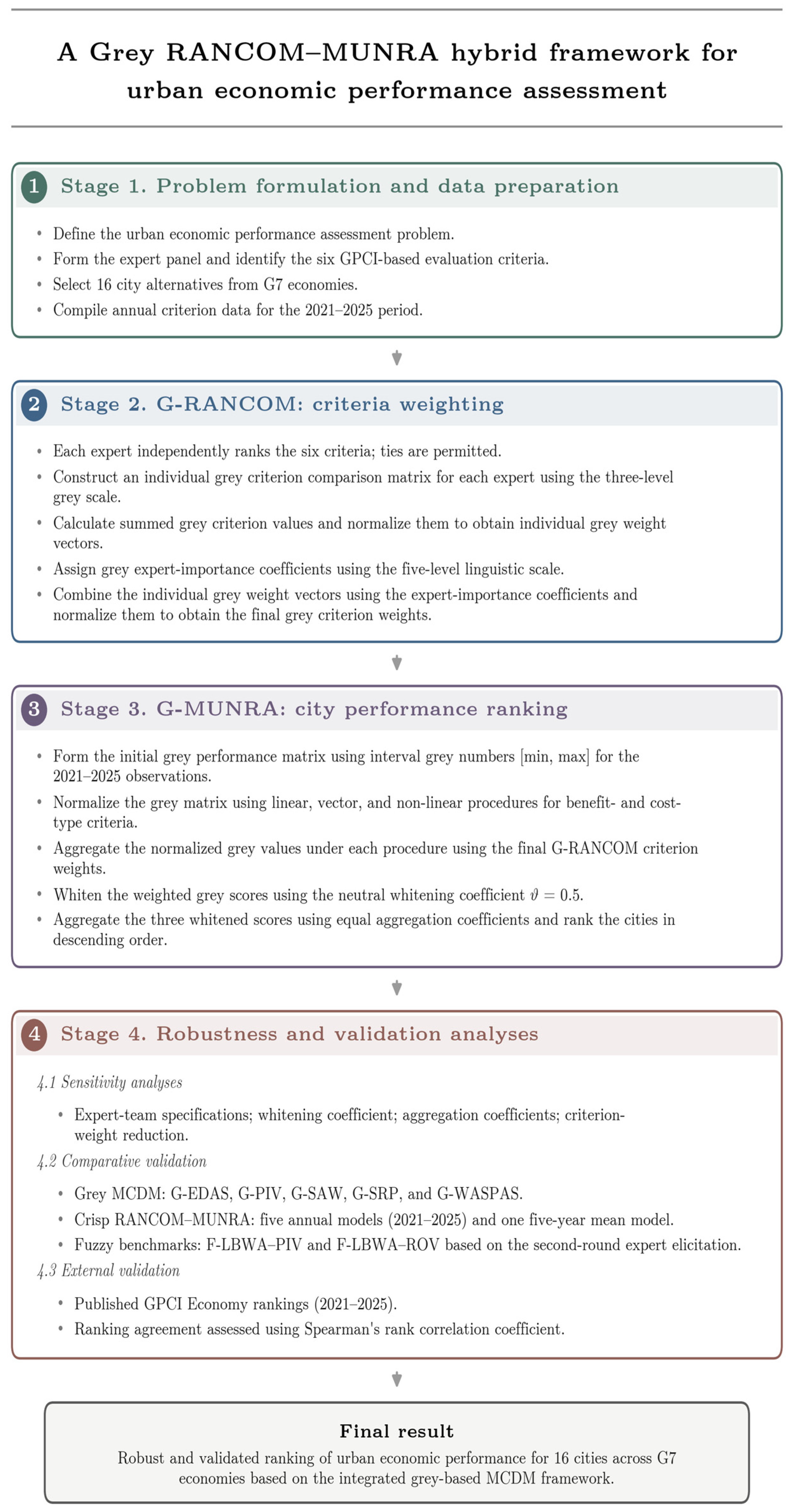
This research employs a hybrid grey group decision-making approach to comparatively assess the economic performance of G7 cities using multi-dimensional urban economic indicators. The methodological framework, illustrated in Figure 1, is designed to handle uncertainty, data heterogeneity, and incomplete information commonly encountered in city-level economic analysis by combining expert judgments with objective secondary data within a grey-system environment. At the outset, the core elements of the decision problem, including the economic performance criteria, city alternatives, and expert committee, are clearly defined. To provide the theoretical basis of the proposed approach, the essential concepts of grey numbers are briefly introduced. The analytical procedure then proceeds in two sequential stages. In the first stage, the G-RANCOM tool identifies the weights of the economic criteria, yielding a set of grey criterion weights that reflect the expert panel’s collective assessments. In the second stage, the G-MUNRA technique derives the final ranking of the G7 cities.

3.1. Grey Numbers

Deng Julong introduced Grey System Theory in the early 1980s to analyze systems characterized by incomplete, limited, or partially observable information. The theory was developed as an alternative to classical deterministic (crisp) and fuzzy-based modelling frameworks, which represent uncertainty either through precise point values or through membership functions. In many decision-making environments, neither exact numerical values nor well-defined membership functions can be reliably specified due to limited data availability or ambiguous expert judgments. Grey system theory addresses this gap by modelling uncertainty through bounded intervals, thereby avoiding the need for probabilistic assumptions or predefined membership structures.

Within this framework, information is classified into three categories by its degree of observability. White information refers to fully known and precisely determined values, whereas black information represents quantities for which no meaningful information is available. Grey information lies between these two extremes and characterizes situations in which exact numerical values are unknown but can be reasonably confined within known lower and upper bounds. Since most decision-making problems involve such partially known information, grey system theory offers a mathematically tractable and conceptually transparent approach to uncertainty modelling. In this context, grey numbers represent uncertainty, preserving interval-based information while avoiding the need for probability density functions or fuzzy membership functions.

3.1.1. Definitions of Grey Numbers [38]

Definition 1.

Grey number

A grey number, denoted by $\otimes v$, is a numerical quantity whose exact value is unknown, while its range of possible values is known.

Definition 2.

Interval grey numbers

A grey number is defined as in Equation (1)

$$\otimes v=\left[v^s,v^b\right], v^s\le v\le v^b$$

(1)

Here, $v^s$ and $v^b$ denote the lower and upper bounds of the grey number, respectively. This interval-based representation explicitly incorporates uncertainty into mathematical modelling while preserving computational simplicity.

3.1.2. Basic Arithmetic Operations of Grey Numbers [23,39]

Let $\otimes v_1=\left[v_1^s,v_1^b\right]$ and $\otimes v_2=\left[v_2^s,v_2^b\right]$ be two interval grey numbers. The fundamental arithmetic operations are defined as follows:

Definition 3.

Addition of grey numbers

The addition of two grey numbers is given by Equation (2)

$$\otimes v_1+\otimes v_2=\left[v_1^s+v_2^s,v_1^b+v_2^b\right]$$

(2)

Definition 4.

Subtraction of grey numbers

The subtraction of two grey numbers is defined in Equation (3).

$$\otimes v_1-\otimes v_2=\left[v_1^s-v_2^b,v_1^b-v_2^s\right]$$

(3)

Definition 5.

Multiplication of grey numbers

The multiplication of two grey numbers is provided in Equation (4)

$$\otimes v_1\times \otimes v_2=\left[\min \left(v_1^s.v_2^s,v_1^s.v_2^b,v_1^b.v_2^s,v_1^b.v_2^b\right),\mathrm{m}\mathrm{a}\mathrm{x}\left(v_1^s.v_2^s,v_1^s.v_2^b,v_1^b.v_2^s,v_1^b.v_2^b\right)\right]$$

(4)

Definition 6.

Division of grey numbers

Provided that $0\notin \otimes v_2$, the division of two grey numbers is formulated in Equation (5).

$$\otimes v_1÷\otimes v_2=\left[min\left({\displaystyle \frac{v_1^s}{v_2^s}},{\displaystyle \frac{v_1^s}{v_2^b}},{\displaystyle \frac{v_1^b}{v_2^s}},{\displaystyle \frac{v_1^b}{v_2^b}}\right),max\left({\displaystyle \frac{v_1^s}{v_2^s}},{\displaystyle \frac{v_1^s}{v_2^b}},{\displaystyle \frac{v_1^b}{v_2^s}},{\displaystyle \frac{v_1^b}{v_2^b}}\right)\right]$$

(5)

3.1.3. Scalar and Functional Operations of Grey Numbers [40]

Beyond basic arithmetic, several scalar and functional operations are defined on grey numbers to support normalization, transformation, and aggregation procedures commonly used in multi-criteria decision-making.

Definition 7.

Scalar multiplication of a grey number

Let $k\in \mathbb{R}$ be a scalar and $\otimes v=\left[v^s,v^b\right]$ be a grey number. Scalar multiplication is expressed in the following equation.

$$k\otimes v=\left\{\begin{array}{c}\left[k{v}^s,k{v}^b\right], k\ge 0\\ \left[k{v}^b,k{v}^s\right], k<0\end{array} \right.$$

(6)

Definition 8.

Power of a grey number

For a non-negative real exponent $E$, the power of a grey number is defined in Equation (7).

$${\left(\otimes v\right)}^p=\left[{\left(v^s\right)}^p,{(v^b)}^p\right], v^s\ge 0$$

(7)

Definition 9.

Inverse of a grey number

If $0\notin \otimes v$, the inverse of a grey number is given by Equation (8).

$${\left(\otimes v\right)}^{-1}=\left[{\displaystyle \frac{1}{v^b}},{\displaystyle \frac{1}{v^s}}\right], v^s\ge 0$$

(8)

3.1.4. Whitenization of Grey Numbers [41]

To enable comparison, aggregation, and ranking, grey numbers are often transformed into crisp values employing a whitenization procedure.

Definition 10.

Whitenization function

For a grey number $\otimes v=\left[v^s,v^b\right]$, the whitened value is defined as:

$$v\left(\vartheta \right)=\left(1-\vartheta \right)v^s+\vartheta v^b, \vartheta \in \left[0,1\right]$$

(9)

The whitenization coefficient $\vartheta$ reflects the decision maker’s attitude toward uncertainty. A neutral assessment is obtained when $\vartheta$= 0.5, which corresponds to the midpoint of the grey interval.

3.2. Grey RANCOM-MUNRA Methodology

3.2.1. Stage 1: Grey Ranking Comparison Method (G-RANCOM) Algorithm for Criterion Weighting

RANCOM is a subjective weighting procedure that identifies the relative importance of criteria solely from ordinal expert judgments [42]. Unlike traditional weighting procedures that rely on extensive pairwise comparisons, the original RANCOM methodology utilizes only ranking information, thereby reducing the cognitive burden on experts and naturally accommodating equal-importance relationships among criteria. In this study, we extend the original RANCOM methodology in two ways. First, we integrate interval grey numbers to explicitly capture the ambiguity and imprecision inherent in expert evaluation. Hence, the importance of a criterion is expressed through lower and upper bounds rather than crisp values. Second, the procedure is implemented individually for each member of the expert panel, and the individual grey weight vectors are combined in the final step using grey expert-importance coefficients. Consequently, the members of the panel do not need to agree on a consensus ranking before the model is run, and the differences in opinion among the experts are not eliminated, but rather preserved as information. A step-by-step explanation of the G-RANCOM technique is provided below. Within the multi-criteria procedure, $C_1,\dots ,C_n$ denote the criteria, whereas $E_1,\dots ,E_T$ indicate the experts participating in the assessment process.

Step 1. Ascertain the ranking order of the criteria.

In this step, the relevant criteria for the decision problem are determined. Each expert $E_t$ then separately ranks the assessment criteria by their relative importance.

Each expert’s judgement is formalized as a ranking function ${\pi }_t$. This ranking function assigns a rank position ${\pi }_t\left(C_i\right)$ to each criterion, where a lower rank reflects higher significance. In situations where criteria are deemed equally important, ties are admissible, indicating that ${\pi }_t\left(C_i\right)={\pi }_t\left(C_j\right)$.

Step 2. Form the grey criterion comparison matrices.

Based on the importance ranking obtained in Step 1, a grey criterion comparison matrix is constructed for every expert $E_t$ as:

$$G_t={\left[\otimes g_{ijt}\right]}_{n\times n},\hspace{0.25em}\hspace{0.25em}\hspace{0.25em}t=1,\dots ,T\hspace{0.25em}$$

(10)

Here, $\otimes g_{ijt}=\left[g_{ijt}^s,g_{ijt}^b\right]$ stands for the grey relative importance of the criterion $C_i$ with respect to $C_j$ as judged by the expert $E_t$ and $g_{ijt}^s$ and $g_{ijt}^b$ denote the lower and upper bounds of the corresponding grey interval, respectively.

The elements of each grey criterion comparison matrix are identified through the use of the grey importance scale detailed in

Table 2. Grey scale utilized in the G-RANCOM comparison matrix.

Relative Importance Relationship	Grey Number
$C_i$ is less important than $C_j.$	[0, $1/3$]
$C_i$ and $C_j$ are equally important.	[1/3, 2/3]
$C_i$ is more important than $C_j.$	[2/3, 1]

. Expert evaluations use a three-level grey linguistic framework based on this scale, which translates ordinal preference information into interval-valued representations. First, the ranking positions ${\pi }_t\left(C_i\right)$ and ${\pi }_t\left(C_j\right)$ are compared to identify the relative significance, which is then assigned to the corresponding grey interval according to the scale in Table 2. In this manner, the comparison matrix systematically encodes whether criterion $C_i$ is assessed as less important than, equally important as, or more important than criterion $C_j$.

Step 3. Calculate the summed grey criteria values.

The elements of each matrix $G_t$ derived in Step 2 are then aggregated in this step to calculate the total values for each criterion. The aggregation is performed independently for each expert employing the matrices associated with them. These values represent intermediate dominance measures derived from the comparison structure and serve as input for the normalization step used to obtain the final grey criterion weights. The summed grey values for each criterion and expert are computed as:

$${\otimes h}_{jt}=\left[h_{jt}^s,h_{jt}^b\right]={\displaystyle \sum _{i=1}^n}\otimes g_{jit}=\left[{\displaystyle \sum _{i=1}^n}{g}_{jit}^s,\hspace{0.25em}{\displaystyle \sum _{i=1}^n}{g}_{jit}^b\right]$$

(11)

In the equation above, elements $\otimes g_{jit}$ constitute the j-th row of $G_t$, where the summation index $i$ extends across the columns.

Step 4. Compute the individual grey weight coefficients.

The grey weight coefficient of criterion $C_j$ under the judgement of expert $E_t$, denoted ${\otimes w}_{jt}$, is computed by normalizing the summed grey criterion value obtained in Step 3 with respect to the total of the summed grey values of that expert.

$${\otimes w}_{jt}=\left[w_{jt}^s,w_{jt}^b\right]=\left[\mathrm{m}\mathrm{i}\mathrm{n}\left({\displaystyle \frac{h_{jt}^s}{{\displaystyle {\sum }_{q=1}^n}{h}_{qt}^s}},{\displaystyle \frac{h_{jt}^b}{{\displaystyle {\sum }_{q=1}^n}{h}_{qt}^b}}\right),\hspace{0.25em}\mathrm{m}\mathrm{a}\mathrm{x}\left({\displaystyle \frac{h_{jt}^s}{{\displaystyle {\sum }_{q=1}^n}{h}_{qt}^s}},{\displaystyle \frac{h_{jt}^b}{{\displaystyle {\sum }_{q=1}^n}{h}_{qt}^b}}\right)\right]$$

(12)

In Equation (12), the summation index $q$ works over the set of criteria, so that the normalization procedure is performed within the opinion of the single expert $E_t$.

Step 5. Assign the grey expert-importance coefficients

Following [43], the importance of expert $E_t$ is expressed as an interval grey number ${\otimes \lambda }_t=\left[{\lambda }_t^s,{\lambda }_t^b\right]$ chosen from the five-level linguistic scale given in

Table 3. Grey scale employed for the expert-importance coefficients.

Linguistic Term	Grey Number
Very unimportant (VUI)	[0.00, 0.20]
Unimportant (UI)	[0.20, 0.40]
Medium important (MI)	[0.40, 0.60]
Important (I)	[0.60, 0.80]
Very important (VI)	[0.80, 1.00]

.

Step 6. Calculate the final grey weight coefficients.

In the last step, each individual weight vector obtained in Step 4 is multiplied by the importance coefficient of the corresponding expert and averaged over the $T$ experts, as formulated in Equation (13). The aggregated values are then normalized via Equation (14) to produce the final grey criterion weights.

$${\otimes z}_j=\left[z_j^s,z_j^b\right]={\displaystyle \frac{1}{T}}{\displaystyle \sum _{t=1}^T}{\otimes \lambda }_t\odot {\otimes w}_{jt}=\left[{\displaystyle \frac{1}{T}}{\displaystyle \sum _{t=1}^T}{\lambda }_t^s{w}_{jt}^s,\hspace{0.25em}{\displaystyle \frac{1}{T}}{\displaystyle \sum _{t=1}^T}{\lambda }_t^b{w}_{jt}^b\right]$$

(13)

$${\otimes w}_j=\left[w_j^s,w_j^b\right]=\left[\mathrm{m}\mathrm{i}\mathrm{n}\left({\displaystyle \frac{z_j^s}{{\displaystyle {\sum }_{q=1}^n}{z}_q^s}},{\displaystyle \frac{z_j^b}{{\displaystyle {\sum }_{q=1}^n}{z}_q^b}}\right),\hspace{0.25em}\mathrm{m}\mathrm{a}\mathrm{x}\left({\displaystyle \frac{z_j^s}{{\displaystyle {\sum }_{q=1}^n}{z}_q^s}},{\displaystyle \frac{z_j^b}{{\displaystyle {\sum }_{q=1}^n}{z}_q^b}}\right)\right]$$

(14)

In Equation (13), $\odot$ stands for the grey multiplication operator. Finally, the grey weight vector calculated based on Equation (14) is used as input in Stage 2.

3.2.2. Stage 2: Grey Multiple Normalization Ranking Analysis (MUNRA) Algorithm for City Ranking

The MUNRA technique is a recent MCDM method introduced by [44] for ranking alternatives by simultaneously using linear, vector, and non-linear normalization procedures. By integrating multiple normalization perspectives within a unified aggregation structure, MUNRA enhances robustness and reduces the sensitivity of ranking results to the choice of a single normalization scheme.

In this research, the classical MUNRA framework is extended into a grey system environment by incorporating interval-valued grey numbers to explicitly model uncertainty and incomplete information inherent in urban economic performance data. The resulting Grey MUNRA (G-MUNRA) tool operates entirely within a grey arithmetic structure, allowing uncertainty to be propagated throughout the normalization, aggregation, and ranking stages. The computational steps of the developed G-MUNRA approach are presented below.

Step 1. Form the initial grey performance matrix $D ={\left[\otimes d_{ij}\right]}_{m\times n}$.

$$D={\left[\begin{array}{ccc}\otimes d_{11}& \otimes d_{12}& \begin{array}{cc}\dots & \otimes d_{1n}\end{array}\\ \otimes d_{21}& \otimes d_{22}& \begin{array}{cc}\dots & \otimes d_{2n}\end{array}\\ \begin{array}{c}⋮\\ \otimes d_{m1}\end{array}& \begin{array}{c}⋮\\ \otimes d_{m2}\end{array}& \begin{array}{c}\begin{array}{cc}\ddots & ⋮\end{array}\\ \begin{array}{cc}\dots & \otimes d_{mn}\end{array}\end{array}\end{array}\right]}_{m\times n}={\left[\begin{array}{ccc}\left[\begin{array}{cc}{d}_{11}^s& d_{11}^b\end{array}\right]& \left[\begin{array}{cc}{d}_{12}^s& d_{12}^b\end{array}\right]& \begin{array}{cc}\dots & \left[\begin{array}{cc}{d}_{1n}^s& d_{1n}^b\end{array}\right]\end{array}\\ \left[\begin{array}{cc}{d}_{21}^s& d_{21}^b\end{array}\right]& \left[\begin{array}{cc}{d}_{22}^s& d_{22}^b\end{array}\right]& \begin{array}{cc}\dots & \left[\begin{array}{cc}{d}_{2n}^s& d_{2n}^b\end{array}\right]\end{array}\\ \begin{array}{c}⋮\\ \left[\begin{array}{cc}{d}_{m1}^s& d_{m1}^b\end{array}\right]\end{array}& \begin{array}{c}⋮\\ \left[\begin{array}{cc}{d}_{m2}^s& d_{m2}^b\end{array}\right]\end{array}& \begin{array}{c}\begin{array}{cc}\ddots & ⋮\end{array}\\ \begin{array}{cc}\dots & \left[\begin{array}{cc}{d}_{mn}^s& d_{mn}^b\end{array}\right]\end{array}\end{array}\end{array}\right]}_{m\times n}$$

(15)

Here, $\otimes d_{ij}= \left[d_{ij}^s,d_{ij}^b\right]$ stands for the grey performance value of the $i^{th}$ city alternative under the $j^{th}$ economic-related criterion. Here, $m$ denotes the number of city alternatives and $n$ the number of criteria.

Step 2: Construct the normalized grey performance matrix $X={\left[{\otimes x}_{ij}\right]}_{m\times n}$.

In this step, the grey performance matrix is normalized using three complementary normalization techniques, namely linear, vector, and non-linear normalization, in order to ensure comparability across criteria with different measurement scales. The normalization procedures are applied separately for benefit-type and cost-type criteria, yielding three normalized grey performance matrices.

In the linear normalization procedure, the normalized grey performance values are computed via Equations (16) and (17). For the vector normalization procedure, Equations (18) and (19) are applied. Finally, non-linear normalization is employed to enhance discrimination among alternatives, with the normalized grey values computed using Equations (20) and (21).

$$\otimes l_{ij}=\left[l_{ij}^s,l_{ij}^b\right]=\left[{\displaystyle \frac{d_{ij}^s}{max\left\{d_{ij}^b|1\le i\le m\right\}}},{\displaystyle \frac{d_{ij}^b}{max\left\{d_{ij}^b|1\le i\le m\right\}}}\right];\forall j\in B$$

(16)

$$\otimes l_{ij}=\left[l_{ij}^s,l_{ij}^b\right]=\left[{\displaystyle \frac{min\left\{d_{ij}^s|1\le i\le m\right\}}{d_{ij}^b}},{\displaystyle \frac{min\left\{d_{ij}^s|1\le i\le m\right\}}{d_{ij}^s}}\right];\forall j\in NB$$

(17)

$$\otimes v_{ij}=\left[v_{ij}^s,v_{ij}^b\right]=\left[{\displaystyle \frac{d_{ij}^s}{\sqrt{{\displaystyle {\sum }_{i=1}^m}{\left(d_{ij}^b\right)}^2}}},{\displaystyle \frac{d_{ij}^b}{\sqrt{{\displaystyle {\sum }_{i=1}^m}{\left(d_{ij}^s\right)}^2}}}\right];\forall j\in B$$

(18)

$$\otimes v_{ij}=\left[v_{ij}^s,v_{ij}^b\right]=\left[1-{\displaystyle \frac{d_{ij}^b}{\sqrt{{\displaystyle {\sum }_{i=1}^m}{\left(d_{ij}^s\right)}^2}}},1-{\displaystyle \frac{d_{ij}^s}{\sqrt{{\displaystyle {\sum }_{i=1}^m}{\left(d_{ij}^b\right)}^2}}}\right];\forall j\in NB$$

(19)

$$\otimes r_{ij}=\left[r_{ij}^s,r_{ij}^b\right]=\left[{\left({\displaystyle \frac{d_{ij}^s}{max\left\{d_{ij}^b|1\le i\le m\right\}}}\right)}^2,{\left({\displaystyle \frac{d_{ij}^b}{max\left\{d_{ij}^b|1\le i\le m\right\}}}\right)}^2\right];\forall j\in B$$

(20)

$$\otimes r_{ij}=\left[r_{ij}^s,r_{ij}^b\right]=\left[{\left({\displaystyle \frac{min\left\{d_{ij}^s|1\le i\le m\right\}}{d_{ij}^b}}\right)}^3,{\left({\displaystyle \frac{min\left\{d_{ij}^s|1\le i\le m\right\}}{d_{ij}^s}}\right)}^3\right];\forall j\in NB$$

(21)

In Equations (16)–(21), $B$ and $NB$ denote the sets of benefit-type and non-benefit-type criteria, respectively.

Step 3. Aggregation of weighted grey scores under each normalization.

After applying the linear, vector, and non-linear normalization procedures, the normalized grey performance values are aggregated using the grey criterion weights computed via Equation (14) of Stage 1. This step performs a weighted aggregation in a grey environment, combining criterion-level contributions to obtain an overall grey performance score for each alternative under each normalization procedure. Thus, the aggregated weighted grey scores for the alternative $A_i$ are computed according to Equations (22)–(24).

$$\otimes L_i^{*}=\left[{\left(l_i^s\right)}^{*},{\left(l_i^b\right)}^{*}\right]=\sum _{j\in B}\otimes l_{ij}\odot {\otimes w}_j+\sum _{j\in NB}\otimes l_{ij}{\odot \otimes w}_j$$

(22)

$$\otimes V_i^{*}=\left[{\left(v_i^s\right)}^{*},{\left(v_i^b\right)}^{*}\right]=\sum _{j\in B}\otimes v_{ij}{\odot \otimes w}_j+\sum _{j\in NB}\otimes v_{ij}{\odot \otimes w}_j$$

(23)

$$\otimes R_i^{*}=\left[{\left(r_i^s\right)}^{*},{\left(r_i^b\right)}^{*}\right]=\sum _{j\in B}\otimes r_{ij}{\odot \otimes w}_j+\sum _{j\in NB}\otimes r_{ij}\odot {\otimes w}_j$$

(24)

Here, the operator $\odot$ denotes grey multiplication, while the summation represents the grey aggregation of criterion-level contributions. The resulting interval-valued scores $\otimes L_i^{*}$, $\otimes V_i^{*}$, and $\otimes R_i^{*}$ preserve uncertainty information and serve as inputs for the subsequent whitenization step.

Step 4. Whitenization of weighted grey scores.

After computing the weighted grey scores from the different normalization schemes, a whitenization step is performed to convert the interval-valued results into crisp scores. To this end, the whitenization operator of Equation (9) is applied at the neutral level $\vartheta$ = 0.5, which reduces it to the midpoint transformation defined in Equations (25)–(27).

$$L_i^{*}={\left(1-\vartheta \right)\left(l_i^s\right)}^{*}+\vartheta {\left(l_i^b\right)}^{*}$$

(25)

$$V_i^{*}={\left(1-\vartheta \right)\left(v_i^s\right)}^{*}+{\vartheta \left(v_i^b\right)}^{*}$$

(26)

$$R_i^{*}=\left(1-\vartheta \right){\left(r_i^s\right)}^{*}+\vartheta {\left(r_i^b\right)}^{*}$$

(27)

Step 5. Final aggregation and ranking.

The final MUNRA score for each city alternative is obtained by aggregating the crisp scores from the three normalization procedures: linear, vector, and non-linear. Accordingly, the overall performance score of the alternative $A_i$ is computed with the aid of Equation (28).

$$S_i={\beta }_1{L}_i^{*}+{\beta }_2{V}_i^{*}+{\beta }_3{R}_i^{*}$$

(28)

In Equation (28), $L_i^{*}$, $V_i^{*}$, and $R_i^{*}$ denote the whitened (crisp) scores obtained from linear, vector, and non-linear normalization procedures, respectively. The aggregation coefficients ${\beta }_1$, ${\beta }_2$, and ${\beta }_3$ satisfy the normalization condition ${\beta }_1+{\beta }_2+{\beta }_3=1$. In the absence of any prior preference regarding the relative contribution of the normalization procedures, equal weights are adopted, such that ${\beta }_1={\beta }_2={\beta }_3=1/3$. Finally, the city alternatives are ranked in descending order of $S_i$, with higher values indicating superior overall economic performance.

4. Case Study: Urban Economic Performance Assessment

A real-world case study is conducted to demonstrate the feasibility and practical relevance of the developed grey group decision-making framework for assessing urban economic performance. The case study focuses on the comparative assessment of selected G7 cities and illustrates how the integrated Grey RANCOM–MUNRA method operates within a complex, data-intensive urban context characterized by uncertainty and heterogeneity.

To implement the case study, a well-defined decision-making problem is formulated. The decision problem is structured around three key components: an expert group, a set of criteria, and a group of city alternatives. The expert team comprises five members who have academic and professional expertise in the fields of economic policy, urban economics, and regional development.

The evaluation criteria comprise six economic performance indicators, all derived from the Global Power City Index (GPCI) framework and representing the core dimensions of urban economic performance. The decision alternatives consist of 16 cities in G7 countries, selected for their global economic significance and the availability of consistent, comparable data across the study period.

This section presents the case study systematically and with methodological consistency. It begins by defining the decision problem the study addresses. It then describes the expert committee involved in the decision-making process. Next, it introduces the economic performance criteria used in the analysis. The next part presents the G7 cities considered as decision alternatives. Finally, the section concludes by implementing the developed grey-based decision support framework.

4.1. Problem Definition

Urban economic performance assessment is an inherently complex MCDM problem because of the multi-dimensional nature of city economies, the heterogeneity of economic indicators, and uncertainty in both data and expert judgments. Cities differ markedly in economic scale, productivity, innovation capacity, labour market dynamics, and global integration, making single-indicator comparisons inadequate and potentially misleading. Consequently, a structured decision-support framework that jointly considers multiple economic dimensions is required to enable transparent and consistent comparative assessment.

In this work, we formulate the decision problem as the comparative assessment and ranking of G7 cities based on their economic performance. The evaluation integrates objective urban economic indicators with expert judgments under uncertainty. Although standardized, internationally comparable data are available, determining the relative importance of economic performance criteria remains nontrivial, particularly when cities exhibit clear trade-offs across economic dimensions.

To overcome these challenges, the problem is embedded in a grey group decision-making environment, where grey interval numbers explicitly represent uncertainty and incomplete information. While the relative importance of economic criteria is determined by considering the independent opinions of each member of the expert committee, city-level performance is evaluated using objective data from GPCI reports for the 2021–2025 period. In this context, this work introduces a hybrid grey RANCOM-MUNRA decision-making methodology that systematically integrates criterion weighting and alternative ranking, enabling the consistent aggregation of expert knowledge and quantitative data while preserving heterogeneity among experts.

4.2. Expert Panel Formation and Elicitation Protocol

The expert committee was formed using purposive sampling after reviewing resumes. Participation required at least 10 years of relevant experience and expertise in fields associated with the assessment problem. We individually invited eight suitable experts via email, summarizing the study’s aim and significance, and five responded by agreeing to participate. Next, we held an individual online meeting with each expert-team member, using standardized information and instructions, to explain the six GPCI-based criteria and the information-gathering procedure. The experts who participated in our research declared no conflict of interest associated with the assessed cities or the organization that provided the data.

Table 4. Profile of the expert panel.

Expert	${\mathit{E}}_1$	${\mathit{E}}_2$	${\mathit{E}}_3$	${\mathit{E}}_4$	${\mathit{E}}_5$
Academic/professional title	Professor	Senior academic researcher	Senior policy expert	Senior researcher	Senior consultant
Area of expertise	Urban and regional economics	Macroeconomic performance analysis	Public policy and urban economic planning	Applied economic analysis and indicators	Strategic urban economics
Degree	PhD	PhD	MSc	PhD	MSc
Experience (Years)	15	14	16	13	18
Institutional background	University	Research institute	Public administration (municipality)	Economic research centre	Consulting/private sector
Linguistic term	Very important (VI)	Medium important (MI)	Important (I)	Medium important (MI)	Important (I)
Grey importance coefficient	[0.80, 1.00]	[0.40, 0.60]	[0.60, 0.80]	[0.40, 0.60]	[0.60, 0.80]

provides detailed information about the expert-team members.

The data collection process consisted of two independent rounds. Round 1 (2–7 August 2026) provided the sequential rankings required for G-RANCOM, while Round 2 (11–14 August 2026) obtained the level-based evaluations needed for the F-LBWA benchmark model. In both rounds, the experts first participated in an individual online meeting, after which the survey was distributed and collected via email. Each expert filled out the forms individually, and the responses were recorded as $E_1-E_5$. Therefore, we recorded differences in opinion as separate information and addressed them through the data collection procedures of the relevant methodologies. Figure A1 summarizes this process, and Appendix B and Appendix G provide the survey content and response instructions.

4.3. Definition of Economic Performance Criteria

In this research, the economic performance of G7 cities is formulated as a multi-criteria decision-making problem comprising six main economic criteria that constitute the evaluation’s analytical structure. These criteria are derived from the GPCI’s economic framework and represent the core aspects through which urban economic performance is defined and assessed [20].

The first criterion, market size $\left({\mathit{C}}_{\mathbf{1}}\right)$, captures the overall scale and productivity of economic activity within a city. It is measured using nominal GDP $\left({\mathit{C}}_{\mathbf{11}}\right)$ and GDP per capita $\left({\mathit{C}}_{\mathbf{12}}\right)$. Nominal GDP reflects the absolute magnitude of economic output and indicates the city’s capacity to sustain large-scale production, consumption, and investment activities. In contrast, GDP per capita captures productivity and income levels, thereby distinguishing cities that are large in scale from those that are economically efficient.

Market attractiveness $\left({\mathit{C}}_{\mathbf{2}}\right)$ reflects the ability of a city to attract investment, firms, and economic activity over time. This criterion is measured via GDP growth rate $\left({\mathit{C}}_{\mathbf{21}}\right)$ and economic freedom $\left({\mathit{C}}_{\mathbf{22}}\right)$. GDP growth rate captures economic dynamism and growth momentum, providing insight into a city’s adaptability and expansion capacity, particularly during periods characterized by economic shocks and subsequent recovery. In addition, economic freedom reflects the institutional and regulatory environment in which economic activities take place, including market openness and regulatory efficiency.

Economic vitality $\left({\mathit{C}}_{\mathbf{3}}\right)$ focuses on the structural depth and global integration of the urban economy. It is captured through stock market capitalization $\left({\mathit{C}}_{\mathbf{31}}\right)$ and the number of the world’s top 500 companies $\left({\mathit{C}}_{\mathbf{32}}\right)$. Stock market capitalization reflects the scale and sophistication of financial markets, indicating the city’s role in capital mobilization and financial intermediation. Furthermore, the presence of the world’s leading firms captures the concentration of corporate headquarters and high-value-added business activities, which are critical for global economic connectivity and strategic decision-making.

Human capital $\left({\mathit{C}}_{\mathbf{4}}\right)$ represents the labour market capacity and skill base of urban economies and is captured through total employment $\left({\mathit{C}}_{\mathbf{41}}\right)$ and employees in business support services $\left({\mathit{C}}_{\mathbf{42}}\right)$. Total employment reflects the city’s ability to generate and sustain jobs, thereby indicating economic scale and labour market inclusiveness. At the same time, employees in business support services capture the concentration of specialized labour supporting advanced economic activities, such as professional, managerial, and corporate services.

Business environment $\left({\mathit{C}}_{\mathbf{5}}\right)$ captures the operational conditions firms face within the city. It is measured using wage levels $\left({\mathit{C}}_{\mathbf{51}}\right)$, the availability of skilled human resources $\left({\mathit{C}}_{\mathbf{52}}\right)$, and the variety of workplace options $\left({\mathit{C}}_{\mathbf{53}}\right)$. Wage level reflects labour cost structures while simultaneously signalling productivity and skill intensity. Moreover, the availability of skilled human resources measures how easily firms can access qualified labour, a key determinant of innovation capacity and business expansion. Finally, the variety of workplace options reflects the diversity and flexibility of working environments, which increasingly influence firm location decisions in knowledge- and service-based urban economies.

The sixth and final criterion, ease of doing business $\left({\mathit{C}}_{\mathbf{6}}\right)$, reflects the regulatory and risk-related conditions affecting economic activity. This criterion is measured by corporate tax rate $\left({\mathit{C}}_{\mathbf{61}}\right)$ and political, economic, and business risk $\left({\mathit{C}}_{\mathbf{62}}\right)$. Corporate tax rate captures the fiscal burden imposed on firms and plays a central role in investment and location decisions. In parallel, political, economic, and business risk reflects the degree of uncertainty faced by economic agents, encompassing macroeconomic stability, institutional reliability, and the overall risk environment.

Of the 13 sub-indicators that make up the six main criteria, 11 are benefit-type indicators in their raw form. The remaining two, the corporate tax rate and the level of political, economic, and business risk, are cost-type indicators by nature. However, the Mori Memorial Foundation applies reverse scoring to these two indicators when computing the published scores. As a result, a lower raw value yields a higher score, and every published sub-indicator and criterion group score is uniformly oriented towards maximization. The sub-indicator scores are then averaged within each criterion group, and the six criterion group scores from the Economy function constitute the criterion values utilized in this research [20].

Table A1. Definition, orientation and transformation of the criteria and sub-indicators.

	Sub-Indicator	Indicator Type	Sign Reversal
Market size ($C_1$)	Nominal GDP ($C_{11}$) Nominal GDP of the city.	Max.	None
	GDP per capita ($C_{12}$) Nominal GDP per capita of the city.	Max.	None
Market attractiveness ($C_2$)	GDP growth rate ($C_{21}$) Five-year compound annual growth rate of the city’s real GDP.	Max.	None
	Level of economic freedom ($C_{22}$) Score of the country in the Heritage Foundation’s Index of Economic Freedom.	Max.	None
Economic vitality ($C_3$)	Stock market capitalization ($C_{31}$) Domestic market capitalization of the stock exchanges located in the city (World Federation of Exchanges).	Max.	None
	Number of the world’s top 500 companies ($C_{32}$) Revenue-weighted score of the Fortune Global 500 firms located within 20 km of the city centre.	Max.	None
Human capital ($C_4$)	Total employment ($C_{41}$) Total employment in the city.	Max.	None
	Employees in business support services ($C_{42}$) Share of employment in finance, insurance, real estate, professional, business and scientific and technical services.	Max.	None
Business environment ($C_5$)	Wage level ($C_{51}$) Average monthly net salary after tax (Numbeo).	Max.	None
	Availability of skilled human resources ($C_{52}$) Composite of the INSEAD Global Talent Competitiveness Index, in its country and city editions, and the EF English Proficiency Index.	Max.	None
	Variety of workplace options ($C_{53}$) Composite of the number of coworking facilities (Coworker.com) and of fixed broadband and mobile connection speeds (Ookla Speedtest).	Max.	None
Ease of doing business ($C_6$)	Corporate tax rate ($C_{61}$) Headline corporate income tax rate applicable to the city (PwC).	Min.	Applied by the GPCI (min→max)
	Level of political, economic and business risk ($C_{62}$) Composite of the World Bank Doing Business indicators, the FM Global Resilience Index and Moody’s long-term country risk ceiling.	Min.	Applied by the GPCI (min→max)

Notes: The text in italics gives the definition of each sub-indicator as published by the data provider.

of Appendix A presents the definition, the type, and the transformation of each sub-indicator.

4.4. Definition of City Alternatives

In this manuscript, we compare urban economic performance across 16 cities in countries commonly referred to as the G7. The G7 economies frame the analysis on three grounds: (i) they account for a large share of global output and host the metropolitan areas in which their financial, corporate, and labour-market functions are concentrated, (ii) they operate under broadly comparable institutional and regulatory conditions, which keeps observed differences attributable to urban economic performance rather than to national development stage, and (iii) the GPCI reports the six Economy function scores for every G7 city it covers in each edition of the 2021–2025 period, so that each grey interval rests on a full five-year series, and all 16 such cities are retained. Detailed information regarding the selected cities is presented in

Table 5. Characteristics of the city alternatives.

Alternative	City	Country	Region
$A_1$	Berlin	Germany	Europe
$A_2$	Boston	USA	North America
$A_3$	Chicago	USA	North America
$A_4$	Frankfurt	Germany	Europe
$A_5$	Fukuoka	Japan	East Asia
$A_6$	London	UK	Europe
$A_7$	Los Angeles	USA	North America
$A_8$	Milan	Italy	Europe
$A_9$	New York	USA	North America
$A_{10}$	Osaka	Japan	East Asia
$A_{11}$	Paris	France	Europe
$A_{12}$	San Francisco	USA	North America
$A_{13}$	Tokyo	Japan	East Asia
$A_{14}$	Toronto	Canada	North America
$A_{15}$	Vancouver	Canada	North America
$A_{16}$	Washington	USA	North America

.

4.5. Implementation of the Developed Approach for Criteria Weight Estimation and City-Level Ranking

4.5.1. Criterion Weighting via the G-RANCOM Method

As shown in Table 4, the expert team combines profiles that differ in seniority and institutional background but share complementary expertise in urban and economic analysis, so the experts receive differentiated grey importance coefficients rather than equal weights. Each member of the expert committee separately ranked the six economic criteria according to the data collection protocol described in Section 4.2. Five separate ranking functions ${\pi }_t$ were retained as separate inputs and reported in

Table 6. Individual criterion rankings of the experts.

	Ordinal preference structure	${\pi }_t\left(C_1\right)$	${\pi }_t\left(C_2\right)$	${\pi }_t\left(C_3\right)$	${\pi }_t\left(C_4\right)$	${\pi }_t\left(C_5\right)$	${\pi }_t\left(C_6\right)$
$E_1$	$C_1\succ C_3=C_5\succ C_4\succ C_2=C_6$	1	4	2	3	2	4
$E_2$	$C_1=C_3\succ C_5\succ C_2=C_4\succ C_6$	1	3	1	3	2	4
$E_3$	$C_3\succ C_1=C_2=C_4=C_5\succ C_6$	2	2	1	2	2	3
$E_4$	$C_1\succ C_2=C_3\succ C_5=C_6\succ C_4$	1	2	2	4	3	3
$E_5$	$C_5\succ C_1=C_2=C_3\succ C_4=C_6$	2	2	2	3	1	3

. Subsequently, the three-level scale in Table 2 was applied to each pair of ranked criteria, and a grey comparison matrix $G_t$ was constructed for each expert utilizing Equation (10). The resulting five matrices are provided in

Table A3. Grey criterion comparison matrix of expert $E_1$.

	${\mathit{C}}_1$		${\mathit{C}}_2$		${\mathit{C}}_3$		${\mathit{C}}_4$		${\mathit{C}}_5$		${\mathit{C}}_6$
$C_1$	0.333	0.667	0.667	1.000	0.667	1.000	0.667	1.000	0.667	1.000	0.667	1.000
$C_2$	0.000	0.333	0.333	0.667	0.000	0.333	0.000	0.333	0.000	0.333	0.333	0.667
$C_3$	0.000	0.333	0.667	1.000	0.333	0.667	0.667	1.000	0.333	0.667	0.667	1.000
$C_4$	0.000	0.333	0.667	1.000	0.000	0.333	0.333	0.667	0.000	0.333	0.667	1.000
$C_5$	0.000	0.333	0.667	1.000	0.333	0.667	0.667	1.000	0.333	0.667	0.667	1.000
$C_6$	0.000	0.333	0.333	0.667	0.000	0.333	0.000	0.333	0.000	0.333	0.333	0.667

,

Table A4. Grey criterion comparison matrix of expert $E_2$.

	${\mathit{C}}_1$		${\mathit{C}}_2$		${\mathit{C}}_3$		${\mathit{C}}_4$		${\mathit{C}}_5$		${\mathit{C}}_6$
$C_1$	0.333	0.667	0.667	1.000	0.333	0.667	0.667	1.000	0.667	1.000	0.667	1.000
$C_2$	0.000	0.333	0.333	0.667	0.000	0.333	0.333	0.667	0.000	0.333	0.667	1.000
$C_3$	0.333	0.667	0.667	1.000	0.333	0.667	0.667	1.000	0.667	1.000	0.667	1.000
$C_4$	0.000	0.333	0.333	0.667	0.000	0.333	0.333	0.667	0.000	0.333	0.667	1.000
$C_5$	0.000	0.333	0.667	1.000	0.000	0.333	0.667	1.000	0.333	0.667	0.667	1.000
$C_6$	0.000	0.333	0.000	0.333	0.000	0.333	0.000	0.333	0.000	0.333	0.333	0.667

,

Table A5. Grey criterion comparison matrix of expert $E_3$.

	${\mathit{C}}_1$		${\mathit{C}}_2$		${\mathit{C}}_3$		${\mathit{C}}_4$		${\mathit{C}}_5$		${\mathit{C}}_6$
$C_1$	0.333	0.667	0.333	0.667	0.000	0.333	0.333	0.667	0.333	0.667	0.667	1.000
$C_2$	0.333	0.667	0.333	0.667	0.000	0.333	0.333	0.667	0.333	0.667	0.667	1.000
$C_3$	0.667	1.000	0.667	1.000	0.333	0.667	0.667	1.000	0.667	1.000	0.667	1.000
$C_4$	0.333	0.667	0.333	0.667	0.000	0.333	0.333	0.667	0.333	0.667	0.667	1.000
$C_5$	0.333	0.667	0.333	0.667	0.000	0.333	0.333	0.667	0.333	0.667	0.667	1.000
$C_6$	0.000	0.333	0.000	0.333	0.000	0.333	0.000	0.333	0.000	0.333	0.333	0.667

,

Table A6. Grey criterion comparison matrix of expert $E_4$.

	${\mathit{C}}_1$		${\mathit{C}}_2$		${\mathit{C}}_3$		${\mathit{C}}_4$		${\mathit{C}}_5$		${\mathit{C}}_6$
$C_1$	0.333	0.667	0.667	1.000	0.667	1.000	0.667	1.000	0.667	1.000	0.667	1.000
$C_2$	0.000	0.333	0.333	0.667	0.333	0.667	0.667	1.000	0.667	1.000	0.667	1.000
$C_3$	0.000	0.333	0.333	0.667	0.333	0.667	0.667	1.000	0.667	1.000	0.667	1.000
$C_4$	0.000	0.333	0.000	0.333	0.000	0.333	0.333	0.667	0.000	0.333	0.000	0.333
$C_5$	0.000	0.333	0.000	0.333	0.000	0.333	0.667	1.000	0.333	0.667	0.333	0.667
$C_6$	0.000	0.333	0.000	0.333	0.000	0.333	0.667	1.000	0.333	0.667	0.333	0.667

and

Table A7. Grey criterion comparison matrix of expert $E_5$.

	${\mathit{C}}_1$		${\mathit{C}}_2$		${\mathit{C}}_3$		${\mathit{C}}_4$		${\mathit{C}}_5$		${\mathit{C}}_6$
$C_1$	0.333	0.667	0.333	0.667	0.333	0.667	0.667	1.000	0.000	0.333	0.667	1.000
$C_2$	0.333	0.667	0.333	0.667	0.333	0.667	0.667	1.000	0.000	0.333	0.667	1.000
$C_3$	0.333	0.667	0.333	0.667	0.333	0.667	0.667	1.000	0.000	0.333	0.667	1.000
$C_4$	0.000	0.333	0.000	0.333	0.000	0.333	0.333	0.667	0.000	0.333	0.333	0.667
$C_5$	0.667	1.000	0.667	1.000	0.667	1.000	0.667	1.000	0.333	0.667	0.667	1.000
$C_6$	0.000	0.333	0.000	0.333	0.000	0.333	0.333	0.667	0.000	0.333	0.333	0.667

of Appendix B.

Table A2. Questionnaire employed in the first elicitation round (G-RANCOM).

	Content
Goal	To obtain the ordinal preference structure of the six criteria.
Material supplied	Definitions of the six GPCI-based criteria and the evaluation problem.
Task	Rank the six criteria based on their importance for assessing the economic performance of a city in a G7 economy. Assign rank 1 to the most important criterion and rank 6 to the least important.
Response format	One integer rank position per criterion, from 1 to 6.
Ties	If you consider two or more criteria equally important, assign them the same rank position.

provides the content and guidelines for the first round of the survey. Summing their rows via Equation (11) produces the summed grey criteria values provided in

Table 7. Summed grey criteria values for each expert.

	$E_1$		$E_2$		$E_3$		$E_4$		$E_5$
	$h_{jt}^s$	$h_{jt}^b$	$h_{jt}^s$	$h_{jt}^b$	$h_{jt}^s$	$h_{jt}^b$	$h_{jt}^s$	$h_{jt}^b$	$h_{jt}^s$	$h_{jt}^b$
$C_1$	3.667	5.667	3.333	5.333	2.000	4.000	3.667	5.667	2.333	4.333
$C_2$	0.667	2.667	1.333	3.333	2.000	4.000	2.667	4.667	2.333	4.333
$C_3$	2.667	4.667	3.333	5.333	3.667	5.667	2.667	4.667	2.333	4.333
$C_4$	1.667	3.667	1.333	3.333	2.000	4.000	0.333	2.333	0.667	2.667
$C_5$	2.667	4.667	2.333	4.333	2.000	4.000	1.333	3.333	3.667	5.667
$C_6$	0.667	2.667	0.333	2.333	0.333	2.333	1.333	3.333	0.667	2.667

. Normalizing these values by Equation (12) yields the individual grey weight vectors given in

Table 8. Individual grey criterion weights.

	$E_1$		$E_2$		$E_3$		$E_4$		$E_5$
	$w_{jt}^s$	$w_{jt}^b$	$w_{jt}^s$	$w_{jt}^b$	$w_{jt}^s$	$w_{jt}^b$	$w_{jt}^s$	$w_{jt}^b$	$w_{jt}^s$	$w_{jt}^b$
$C_1$	0.236	0.306	0.222	0.278	0.167	0.167	0.236	0.306	0.181	0.194
$C_2$	0.056	0.111	0.111	0.139	0.167	0.167	0.194	0.222	0.181	0.194
$C_3$	0.194	0.222	0.222	0.278	0.236	0.306	0.194	0.222	0.181	0.194
$C_4$	0.139	0.153	0.111	0.139	0.167	0.167	0.028	0.097	0.056	0.111
$C_5$	0.194	0.222	0.181	0.194	0.167	0.167	0.111	0.139	0.236	0.306
$C_6$	0.056	0.111	0.028	0.097	0.028	0.097	0.111	0.139	0.056	0.111

. Next, the individual vectors are integrated through Equation (13), employing the grey expert-importance coefficients in the last two rows of Table 4, and the aggregate is normalized with the help of Equation (14). The final grey criterion weight values are given in

Table 9. Final grey weights.

	$z_j^s$	$z_j^b$	$w_j^s$	$w_j^b$	Rank
$C_1$	0.1161	0.1889	0.224	0.233	1
$C_2$	0.0750	0.1233	0.146	0.151	4
$C_3$	0.1144	0.1844	0.219	0.230	2
$C_4$	0.0600	0.1033	0.120	0.122	5
$C_5$	0.1028	0.1600	0.190	0.206	3
$C_6$	0.0300	0.0839	0.060	0.099	6

.

The five ranking functions are not identical, so their agreement is quantified before aggregation. Kendall’s coefficient of concordance, computed on the mid-ranks of Table 6 with the standard correction for ties, equals W = 0.656 (χ²(5) = 16.40, p = 0.006), and the mean pairwise Spearman correlation is 0.568, ranging from 0.348 to 0.909. Agreement on the overall importance structure is therefore substantial and statistically significant, while divergence on individual criteria remains. Since consensus was not imposed (Section 4.2), this divergence is retained as information and carried by the grey intervals of the weight vector, and Section 5.1 indicates that it does not significantly influence the final ranking.

4.5.2. Ranking City Alternatives Employing the Grey MUNRA Method

Table 10. Grey performance matrix for city alternatives.

	$C_1$		$C_2$		$C_3$		$C_4$		$C_5$		$C_6$
$A_1$	16.90	20.80	46.30	68.00	0.60	0.60	38.40	39.60	41.40	49.90	49.50	53.00
$A_2$	26.10	40.30	47.60	56.30	1.60	2.60	18.20	21.00	69.00	84.10	57.80	62.60
$A_3$	25.60	29.70	38.40	45.00	1.70	2.30	30.50	32.80	59.90	71.30	56.10	60.40
$A_4$	24.00	29.60	33.80	45.80	3.20	4.10	47.90	52.00	41.10	46.90	46.90	49.70
$A_5$	8.20	13.00	29.50	45.10	0.00	0.50	28.60	36.30	8.80	34.80	47.20	52.10
$A_6$	45.60	57.50	34.50	58.10	13.40	17.50	66.40	70.50	63.60	80.80	66.70	69.70
$A_7$	30.70	35.20	42.70	53.40	0.70	0.90	28.20	31.10	68.20	79.10	55.10	59.60
$A_8$	15.80	18.90	21.60	35.10	0.00	1.30	34.00	53.20	28.00	34.90	42.20	48.30
$A_9$	71.20	80.70	44.10	53.60	60.20	63.90	42.00	42.90	78.80	92.30	49.00	50.80
$A_{10}$	16.50	24.70	28.10	42.00	2.90	4.00	35.90	43.80	17.90	36.10	47.70	51.00
$A_{11}$	37.20	44.20	22.90	40.70	16.90	21.90	44.90	48.10	49.10	56.50	50.20	60.20
$A_{12}$	35.20	58.90	53.60	75.10	0.80	2.30	25.10	29.00	75.50	83.90	56.80	61.40
$A_{13}$	47.20	63.60	29.60	44.60	24.40	30.50	58.70	68.10	31.50	46.30	46.90	50.30
$A_{14}$	14.80	18.20	42.10	60.70	5.90	8.20	42.40	51.20	62.50	64.80	54.80	60.00
$A_{15}$	10.50	12.10	50.60	71.60	0.00	0.00	37.10	42.70	54.50	63.90	54.10	59.10
$A_{16}$	54.60	57.30	42.60	51.60	4.00	6.60	17.80	19.30	63.20	80.80	57.50	62.30

presents the grey performance matrix $D={\left[\otimes d_{ij}\right]}_{16\times 6}$ formed for the city alternatives. For each city alternative and criterion, the minimum and maximum GPCI scores observed during 2021–2025 are used as the lower and upper limits of the corresponding grey number, respectively. Accordingly, this grey matrix reports each city’s interval-valued performance across the six criteria, capturing temporal variability and cross-city heterogeneity in urban economic indicators derived from the GPCI datasets. Performance values of city alternatives for each criterion during 2021–2025 are presented in

Table A8. Annual criteria scores for city alternatives.

Code	City	Year	${\mathit{C}}_1$	${\mathit{C}}_2$	${\mathit{C}}_3$	${\mathit{C}}_4$	${\mathit{C}}_5$	${\mathit{C}}_6$
$A_1$	Berlin	2021	19.40	50.30	0.60	38.40	49.20	49.70
		2022	18.40	54.40	0.60	38.70	49.90	49.80
		2023	18.40	68.00	0.60	39.60	46.70	49.50
		2024	20.80	56.60	0.60	38.80	41.50	53.00
		2025	16.90	46.30	0.60	38.50	41.40	53.00
$A_2$	Boston	2021	26.70	48.90	2.60	19.70	69.30	57.80
		2022	27.40	53.80	2.20	20.50	69.00	57.90
		2023	26.10	56.30	2.20	21.00	74.80	57.80
		2024	40.30	50.80	1.60	19.50	84.10	62.60
		2025	39.50	47.60	1.70	18.20	69.90	62.60
$A_3$	Chicago	2021	27.40	41.10	2.30	30.50	64.10	56.10
		2022	27.00	45.00	2.20	32.70	65.40	56.20
		2023	25.60	43.90	2.10	32.80	67.90	56.10
		2024	29.70	44.40	1.70	31.90	71.30	60.40
		2025	28.40	38.40	1.90	30.80	59.90	60.40
$A_4$	Frankfurt	2021	28.20	33.80	4.00	52.00	45.90	47.10
		2022	29.60	39.60	4.10	51.40	46.90	47.20
		2023	27.60	45.80	4.00	50.10	46.60	46.90
		2024	28.70	45.40	3.20	48.70	43.20	49.70
		2025	24.00	37.10	3.30	47.90	41.10	49.70
$A_5$	Fukuoka	2021	13.00	36.40	0.50	28.60	28.10	47.50
		2022	12.90	45.10	0.30	28.70	33.40	47.60
		2023	12.40	42.10	0.30	36.30	34.80	47.20
		2024	11.40	29.50	0.00	35.30	15.90	50.60
		2025	8.20	34.50	0.00	35.10	8.80	52.10
$A_6$	London	2021	53.50	53.20	17.50	70.50	63.60	69.60
		2022	49.30	58.10	13.40	69.40	66.80	69.70
		2023	47.10	46.70	14.00	66.40	80.80	69.60
		2024	57.50	49.20	13.70	69.50	79.70	66.70
		2025	45.60	34.50	14.10	68.30	77.10	66.70
$A_7$	Los Angeles	2021	34.30	50.60	0.70	29.70	70.70	55.20
		2022	33.80	53.40	0.70	31.10	68.20	55.30
		2023	30.70	51.90	0.70	31.10	69.90	55.10
		2024	35.20	48.80	0.80	29.10	79.10	59.60
		2025	33.30	42.70	0.90	28.20	72.10	59.60
$A_8$	Milan	2021	17.90	21.60	1.30	34.00	29.80	48.30
		2022	18.90	35.10	1.00	34.20	34.90	42.70
		2023	16.40	31.90	0.90	52.90	32.70	42.20
		2024	18.20	32.10	0.00	53.00	29.30	46.80
		2025	15.80	28.70	1.30	53.20	28.00	46.80
$A_9$	New York	2021	76.80	51.50	60.70	42.90	81.80	49.10
		2022	80.70	51.40	60.20	42.60	81.40	49.10
		2023	78.50	53.60	60.40	42.20	78.80	49.00
		2024	73.00	51.60	61.30	42.20	92.30	50.80
		2025	71.20	44.10	63.90	42.00	81.60	50.80
$A_{10}$	Osaka	2021	24.70	28.10	4.00	35.90	31.10	47.90
		2022	23.10	42.00	3.80	36.00	29.10	48.00
		2023	23.10	40.30	3.40	43.80	36.10	47.70
		2024	23.70	29.80	2.90	42.70	24.20	51.00
		2025	16.50	34.40	2.90	42.00	17.90	51.00
$A_{11}$	Paris	2021	37.40	22.90	21.80	47.50	50.50	50.20
		2022	43.40	37.00	16.90	48.10	56.50	52.50
		2023	40.90	40.70	18.70	46.20	54.50	52.10
		2024	44.20	35.10	19.60	44.90	49.10	60.20
		2025	37.20	29.60	21.90	45.60	49.10	60.20
$A_{12}$	San Francisco	2021	35.20	65.00	1.10	27.60	83.90	56.80
		2022	37.10	66.60	0.80	28.90	82.00	56.90
		2023	35.90	75.10	0.80	29.00	83.70	56.80
		2024	58.90	59.40	1.40	27.80	82.70	61.40
		2025	58.30	53.60	2.30	25.10	75.50	61.40
$A_{13}$	Tokyo	2021	61.90	33.10	30.50	58.70	42.20	47.20
		2022	58.10	42.30	27.80	58.90	46.30	47.30
		2023	61.10	44.60	26.10	68.10	45.20	46.90
		2024	63.60	29.60	24.40	67.00	35.30	50.30
		2025	47.20	29.60	25.00	67.90	31.50	50.30
$A_{14}$	Toronto	2021	17.00	51.80	7.10	47.00	62.50	55.00
		2022	16.30	57.80	6.50	47.20	64.80	55.10
		2023	14.80	60.70	5.90	45.50	64.30	54.80
		2024	18.20	59.60	6.30	42.40	62.60	60.00
		2025	16.30	42.10	8.20	51.20	63.30	60.00
$A_{15}$	Vancouver	2021	11.10	56.30	0.00	42.70	59.90	54.30
		2022	11.00	61.90	0.00	38.40	60.70	54.40
		2023	10.50	71.60	0.00	37.10	63.50	54.10
		2024	12.10	64.80	0.00	39.40	63.90	59.10
		2025	11.40	50.60	0.00	38.80	54.50	59.10
$A_{16}$	Washington, DC	2021	56.80	43.40	4.20	18.60	76.30	57.50
		2022	55.80	48.10	4.00	19.10	74.20	57.60
		2023	56.00	51.60	4.00	19.30	76.10	57.50
		2024	57.30	46.40	5.60	18.90	80.80	62.30
		2025	54.60	42.60	6.60	17.80	63.20	62.30

of Appendix C.

Based on the grey performance matrix given in Table 10, the normalized grey performance matrices are formed in accordance with the normalization procedures defined in Equations (16)–(21). Specifically,

Table 11. Linear normalization.

	$C_1$		$C_2$		$C_3$		$C_4$		$C_5$		$C_6$
$A_1$	0.209	0.258	0.617	0.905	0.009	0.009	0.545	0.562	0.449	0.541	0.710	0.760
$A_2$	0.323	0.499	0.634	0.750	0.025	0.041	0.258	0.298	0.748	0.911	0.829	0.898
$A_3$	0.317	0.368	0.511	0.599	0.027	0.036	0.433	0.465	0.649	0.772	0.805	0.867
$A_4$	0.297	0.367	0.450	0.610	0.050	0.064	0.679	0.738	0.445	0.508	0.673	0.713
$A_5$	0.102	0.161	0.393	0.601	0.000	0.008	0.406	0.515	0.095	0.377	0.677	0.747
$A_6$	0.565	0.713	0.459	0.774	0.210	0.274	0.942	1.000	0.689	0.875	0.957	1.000
$A_7$	0.380	0.436	0.569	0.711	0.011	0.014	0.400	0.441	0.739	0.857	0.791	0.855
$A_8$	0.196	0.234	0.288	0.467	0.000	0.020	0.482	0.755	0.303	0.378	0.605	0.693
$A_9$	0.882	1.000	0.587	0.714	0.942	1.000	0.596	0.609	0.854	1.000	0.703	0.729
$A_{10}$	0.204	0.306	0.374	0.559	0.045	0.063	0.509	0.621	0.194	0.391	0.684	0.732
$A_{11}$	0.461	0.548	0.305	0.542	0.264	0.343	0.637	0.682	0.532	0.612	0.720	0.864
$A_{12}$	0.436	0.730	0.714	1.000	0.013	0.036	0.356	0.411	0.818	0.909	0.815	0.881
$A_{13}$	0.585	0.788	0.394	0.594	0.382	0.477	0.833	0.966	0.341	0.502	0.673	0.722
$A_{14}$	0.183	0.226	0.561	0.808	0.092	0.128	0.601	0.726	0.677	0.702	0.786	0.861
$A_{15}$	0.130	0.150	0.674	0.953	0.000	0.000	0.526	0.606	0.590	0.692	0.776	0.848
$A_{16}$	0.677	0.710	0.567	0.687	0.063	0.103	0.252	0.274	0.685	0.875	0.825	0.894

presents the results of linear normalization obtained using Equation (16),

Table 12. Vector normalization.

	$C_1$		$C_2$		$C_3$		$C_4$		$C_5$		$C_6$
$A_1$	0.099	0.151	0.214	0.434	0.008	0.009	0.214	0.251	0.158	0.228	0.216	0.251
$A_2$	0.153	0.292	0.220	0.359	0.021	0.038	0.101	0.133	0.263	0.385	0.253	0.297
$A_3$	0.150	0.215	0.177	0.287	0.022	0.033	0.170	0.208	0.228	0.326	0.245	0.286
$A_4$	0.140	0.215	0.156	0.292	0.041	0.059	0.267	0.330	0.156	0.214	0.205	0.236
$A_5$	0.048	0.094	0.136	0.288	0.000	0.007	0.159	0.230	0.033	0.159	0.206	0.247
$A_6$	0.267	0.417	0.159	0.371	0.174	0.254	0.370	0.447	0.242	0.370	0.291	0.330
$A_7$	0.180	0.255	0.197	0.341	0.009	0.013	0.157	0.197	0.260	0.362	0.241	0.283
$A_8$	0.092	0.137	0.100	0.224	0.000	0.019	0.189	0.338	0.107	0.160	0.184	0.229
$A_9$	0.416	0.585	0.204	0.342	0.780	0.926	0.234	0.272	0.300	0.422	0.214	0.241
$A_{10}$	0.096	0.179	0.130	0.268	0.038	0.058	0.200	0.278	0.068	0.165	0.208	0.242
$A_{11}$	0.218	0.320	0.106	0.260	0.219	0.317	0.250	0.305	0.187	0.258	0.219	0.285
$A_{12}$	0.206	0.427	0.248	0.479	0.010	0.033	0.140	0.184	0.287	0.384	0.248	0.291
$A_{13}$	0.276	0.461	0.137	0.285	0.316	0.442	0.327	0.432	0.120	0.212	0.205	0.238
$A_{14}$	0.087	0.132	0.195	0.388	0.076	0.119	0.236	0.325	0.238	0.296	0.239	0.284
$A_{15}$	0.061	0.088	0.234	0.457	0.000	0.000	0.207	0.271	0.207	0.292	0.236	0.280
$A_{16}$	0.319	0.415	0.197	0.329	0.052	0.096	0.099	0.122	0.240	0.370	0.251	0.295

reports the vector-normalized grey performance matrix obtained using Equation (18), and

Table 13. Non-linear normalization.

	$C_1$		$C_2$		$C_3$		$C_4$		$C_5$		$C_6$
$A_1$	0.044	0.066	0.380	0.820	0.000	0.000	0.297	0.316	0.201	0.292	0.504	0.578
$A_2$	0.105	0.249	0.402	0.562	0.001	0.002	0.067	0.089	0.559	0.830	0.688	0.807
$A_3$	0.101	0.135	0.261	0.359	0.001	0.001	0.187	0.216	0.421	0.597	0.648	0.751
$A_4$	0.088	0.135	0.203	0.372	0.003	0.004	0.462	0.544	0.198	0.258	0.453	0.508
$A_5$	0.010	0.026	0.154	0.361	0.000	0.000	0.165	0.265	0.009	0.142	0.459	0.559
$A_6$	0.319	0.508	0.211	0.599	0.044	0.075	0.887	1.000	0.475	0.766	0.916	1.000
$A_7$	0.145	0.190	0.323	0.506	0.000	0.000	0.160	0.195	0.546	0.734	0.625	0.731
$A_8$	0.038	0.055	0.083	0.218	0.000	0.000	0.233	0.569	0.092	0.143	0.367	0.480
$A_9$	0.778	1.000	0.345	0.509	0.888	1.000	0.355	0.370	0.729	1.000	0.494	0.531
$A_{10}$	0.042	0.094	0.140	0.313	0.002	0.004	0.259	0.386	0.038	0.153	0.468	0.535
$A_{11}$	0.212	0.300	0.093	0.294	0.070	0.117	0.406	0.465	0.283	0.375	0.519	0.746
$A_{12}$	0.190	0.533	0.509	1.000	0.000	0.001	0.127	0.169	0.669	0.826	0.664	0.776
$A_{13}$	0.342	0.621	0.155	0.353	0.146	0.228	0.693	0.933	0.116	0.252	0.453	0.521
$A_{14}$	0.034	0.051	0.314	0.653	0.009	0.016	0.362	0.527	0.459	0.493	0.618	0.741
$A_{15}$	0.017	0.022	0.454	0.909	0.000	0.000	0.277	0.367	0.349	0.479	0.602	0.719
$A_{16}$	0.458	0.504	0.322	0.472	0.004	0.011	0.064	0.075	0.469	0.766	0.681	0.799

presents the non-linear normalization results obtained using Equation (20).

After normalization, the weighted aggregation of the grey performance values is performed using the G-MUNRA technique defined in Equations (22)–(24). For each normalization structure, criterion-level grey values were multiplied by the corresponding grey weights and subsequently aggregated to obtain alternative-level grey scores. These aggregated grey scores are then transformed into crisp values through the whitenization procedure specified in Equations (25)–(27), yielding representative scores for linear, vector, and non-linear normalization. Finally, we computed the overall performance score for each city alternative by aggregating the whitened scores using Equation (28), with equal aggregation coefficients for the three normalization procedures.

Table 14. Final grey MUNRA outcomes.

	$\otimes L_i^{*}$		$\otimes V_i^{*}$		$\otimes R_i^{*}$		$L_i^{*}$	$V_i^{*}$	$R_i^{*}$	$S_i$	Rank
$A_1$	0.3324	0.4544	0.1237	0.2053	0.1696	0.2953	0.393	0.165	0.232	0.263	13
$A_2$	0.3932	0.5522	0.1480	0.2559	0.2376	0.4053	0.473	0.202	0.321	0.332	7
$A_3$	0.3751	0.4866	0.1427	0.2222	0.2023	0.3101	0.431	0.182	0.256	0.290	10
$A_4$	0.3500	0.4580	0.1374	0.2157	0.1704	0.2587	0.404	0.177	0.215	0.265	12
$A_5$	0.1878	0.3448	0.0686	0.1525	0.0740	0.1777	0.266	0.111	0.126	0.168	16
$A_6$	0.5411	0.7477	0.2289	0.3750	0.3639	0.6055	0.644	0.302	0.485	0.477	2
$A_7$	0.4065	0.5276	0.1536	0.2406	0.2401	0.3685	0.467	0.197	0.304	0.323	8
$A_8$	0.2379	0.3689	0.0894	0.1670	0.0882	0.1927	0.303	0.128	0.140	0.191	15
$A_9$	0.7651	0.9233	0.3913	0.5448	0.6293	0.8437	0.844	0.468	0.737	0.683	1
$A_{10}$	0.2496	0.3993	0.0983	0.1875	0.0968	0.2018	0.324	0.143	0.149	0.206	14
$A_{11}$	0.4264	0.5835	0.1907	0.3057	0.2102	0.3495	0.505	0.248	0.280	0.344	6
$A_{12}$	0.4517	0.6542	0.1708	0.3099	0.2992	0.5432	0.553	0.240	0.421	0.405	4
$A_{13}$	0.4774	0.6761	0.2253	0.3720	0.2640	0.4680	0.577	0.299	0.366	0.414	3
$A_{14}$	0.3913	0.5230	0.1524	0.2455	0.2230	0.3539	0.457	0.199	0.288	0.315	9
$A_{15}$	0.3496	0.4797	0.1264	0.2105	0.2059	0.3573	0.415	0.168	0.282	0.288	11
$A_{16}$	0.4579	0.5955	0.1842	0.2889	0.2879	0.4376	0.527	0.237	0.363	0.375	5

summarizes the resulting G-MUNRA scores and rankings. Based on Table 14, the final ranking of city alternatives is $A_9\succ A_6\succ A_{13}\succ A_{12}\succ A_{16}\succ A_{11}\succ A_2\succ A_7\succ A_{14}\succ A_3\succ A_{15}\succ A_4\succ A_1\succ A_{10}\succ A_8\succ A_5$.

4.6. Redundancy and Collinearity of the Criterion Set

The six criteria are drawn from the GPCI’s economic framework [20] and are conceptually distinct from one another by their very nature. However, because they define different aspects of the same urban economies, a certain statistical relationship between them is expected.

Table 15. Pearson correlation matrix.

	$C_1$	$C_2$	$C_3$	$C_4$	$C_5$	$C_6$
$C_1$	1.000	0.070	0.767	0.136	0.588	0.237
$C_2$		1.000	−0.098	−0.322	0.631	0.491
$C_3$			1.000	0.377	0.310	−0.149
$C_4$				1.000	−0.267	−0.114
$C_5$					1.000	0.696
$C_6$						1.000

displays the Pearson correlation coefficients calculated across 16 city alternatives based on the midpoints of the grey performance intervals in Table 10. As shown in Table 15, the highest correlation coefficients between criterion pairs were calculated as 0.767 ($C_1-C_3$) and 0.696 ($C_5-C_6$). No pair reaches 0.8, which is considered an indicator of redundancy. This result is not affected by the chosen representative value. When the analysis is repeated using lower bounds, upper bounds, and the five-year averages in Appendix C instead of midpoints, the strongest pair remains $C_1$ and $C_3$ in every case, while the corresponding correlations—0.774, 0.748, and 0.773—remain below the 0.8 threshold. Replacing the metric with a rank-based equivalent also does not alter this conclusion, since the maximum absolute Spearman correlation based on midpoints is 0.729.

Bivariate correlation captures only the relationship between two variables. Therefore, a criterion may be close to a linear combination of the others even though none of the individual correlations is high.

Table 16. Auxiliary regression diagnostics.

	${\mathit{R}}^2$	Adjusted ${\mathit{R}}^2$	VIF	Adjusted VIF
$C_1$	0.757	0.636	4.12	2.75
$C_2$	0.545	0.317	2.20	1.46
$C_3$	0.808	0.713	5.22	3.48
$C_4$	0.494	0.242	1.98	1.32
$C_5$	0.862	0.793	7.25	4.83
$C_6$	0.746	0.619	3.93	2.62

addresses this multivariate aspect through auxiliary regressions in which each criterion is regressed on the remaining five criteria. The variance inflation factors (VIF) range from 1.98 for $C_4$ to 7.25 for $C_5$, indicating that none of the criteria approaches the threshold of 10 traditionally used to indicate severe multicollinearity. Since only 16 observations are available for five regressors in each auxiliary regression, $R^2$ is biassed upward, and the reported factors therefore overstate rather than understate collinearity, with the corresponding values obtained from Adj. $R^2$ ranging from 1.32 to 4.83.

When the findings from Table 15 and Table 16 are considered together, it is observed that no single criterion duplicates the information provided by the others, either individually or collectively. However, the diagnostics do describe this specific sample, and the statistical relationship does not imply preferential dependence. The contribution of each criterion to the initial ranking is further tested with the weighting scenarios described in Section 5.2. These results support using the additive aggregation of G-MUNRA in the present application.

5. Sensitivity and Comparative Robustness Analyses

The following section presents the sensitivity analysis of the ranking positions derived through the introduced grey hybrid methodology and validates the initial outcomes. For the sensitivity analyses, we explored the influence of variations in the model’s parameters and weight values on the initial ranking positions, first one parameter at a time and then jointly over the entire admissible parameter space. In addition, the validity of the initial outcomes was tested by comparing rankings from the developed grey decision support tool with those from existing grey-based models, deterministic (crisp) models, fuzzy logic-based models, and the GPCI Economy rankings. In all comparisons, we measured agreement between the two rankings using Spearman’s rank correlation coefficient.

5.1. Sensitivity Analysis—Variation in the Model Parameters ${\otimes \lambda }_t$, $\vartheta$ and $\beta$

The introduced decision support model comprises three parameters: the grey importance coefficients ${\otimes \lambda }_t$ $(t = 1, \dots , 5)$, which aggregate expert opinions within G-RANCOM; the whitenization coefficient $\vartheta$ in the G-MUNRA procedure; and the aggregation coefficients $\beta =({\beta }_1,{\beta }_2,{\beta }_3)$, which govern the contributions of the three normalizations in the G-MUNRA model.

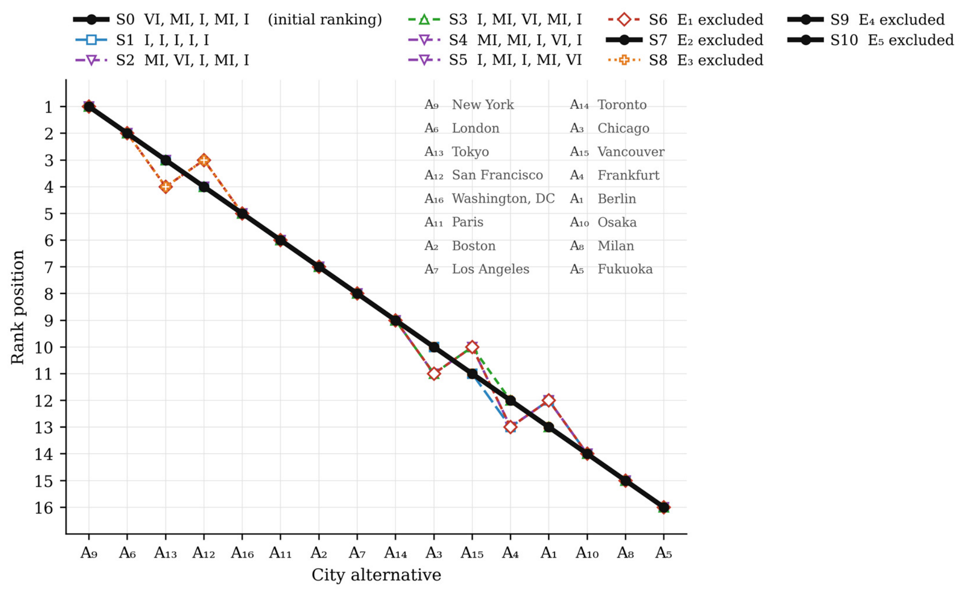
First, we develop 10 scenarios to analyze the effect of the grey importance coefficients, which determine the weights assigned to experts in the initial ranking results. In S1, all experts have the same level of importance, and the value “I” is assigned to all five experts as a linguistic variable. In S2–S5, the most important linguistic term, VI, is assigned to the remaining four experts, respectively, excluding the first expert. In S6–S10, we exclude one expert at a time. Figure 2 shows the ranking results for all scenarios. As shown in Figure 2, the 10 scenarios produce six different rankings. The Spearman correlation coefficients (SCCs) between the scenario rankings and the initial ranking results range from 0.9912 to 1.0000. In all scenarios, the first two and last three ranks remain unchanged, and in any given scenario, no city alternative changes its rank by more than one position.

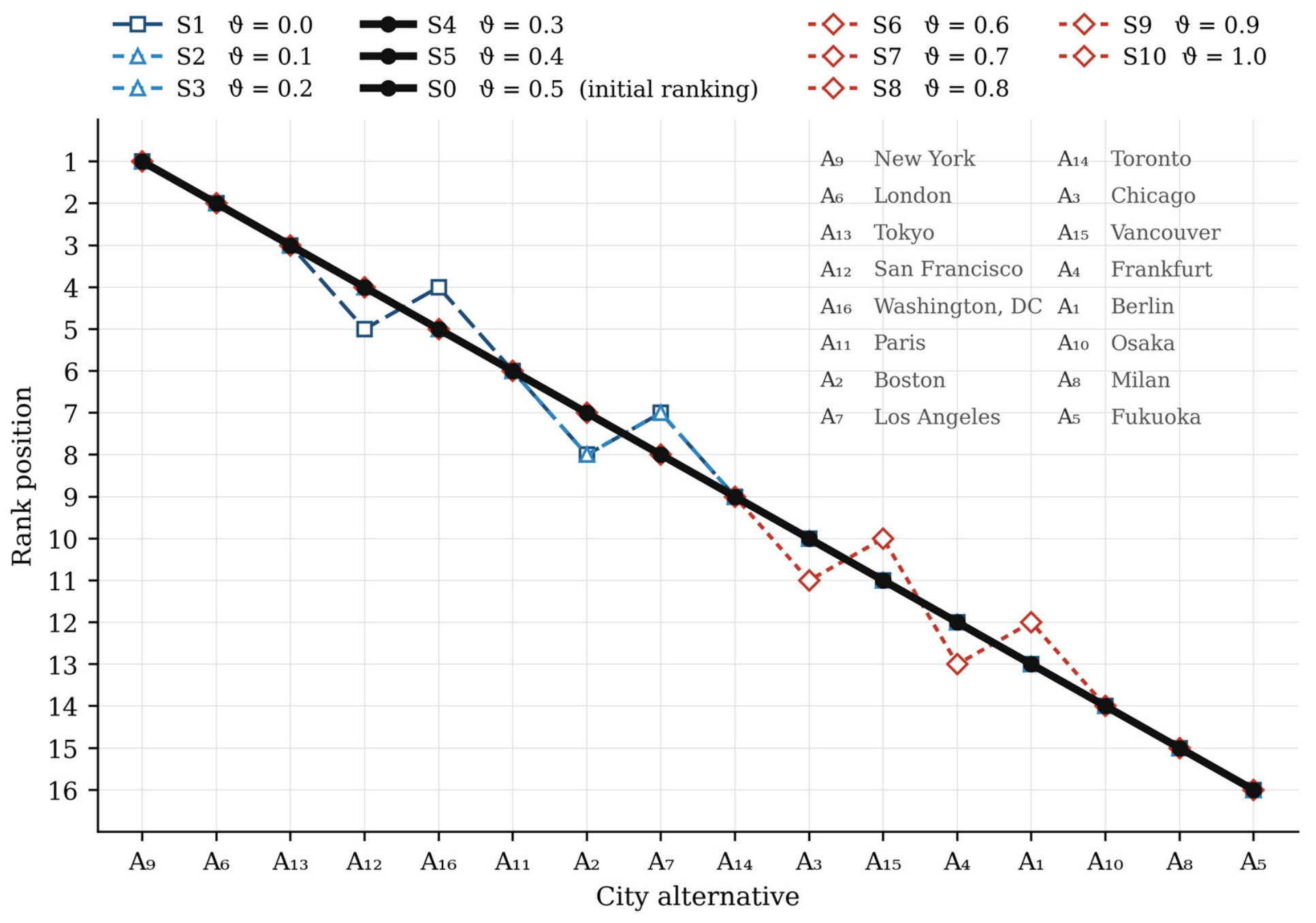
Second, the whitenization coefficient $\vartheta \in [0,1]$ is set to 0.5 to obtain the initial ranking positions. In this part, ten scenarios are designed to evaluate the influence of $\vartheta$ on the initial ranking results of G-MUNRA. In the first scenario, the $\vartheta$ parameter is set to 0, while in the last scenario, it increases in increments of 0.10 until it reaches 1. The results of the scenarios associated with the $\vartheta$ parameter are illustrated in Figure 3. Although the 10 scenarios produce three different rankings, the SCCs between the scenario rankings and the initial ranking range from 0.9941 to 1.0000. In all scenarios, the top three and bottom three positions remain unchanged.

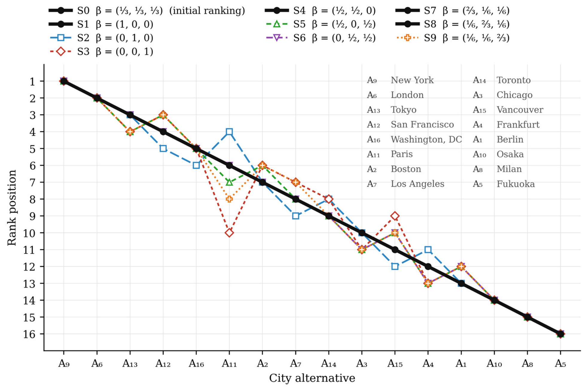
Third, nine scenarios are formulated to explore the impact of variations in the aggregation-coefficient vector $\beta$, which integrates the outcomes of three different normalizations subject to ${\beta }_1 + {\beta }_2 + {\beta }_3 = 1$. The nine scenarios are formed based on an augmented simplex-centroid design over the unit simplex: three pure vertices (S1–S3), three binary mixtures (S4–S6), and three axial points (S7–S9). Figure 4 shows the ranking results from the nine formulated scenarios. As shown in Figure 4, implementing the scenarios yields six separate rankings. The computed correlations between the initial ranking and the scenario rankings range from 0.9588 to 1.0000. $A_9$, $A_6$, $A_5$, $A_8$, and $A_{10}$ are the five alternatives that retain their ranking positions in all nine scenarios. However, the alternative with the greatest variation in ranking position is $A_{11}$. Across all scenarios, this alternative’s ranking position varies between 4 and 10.

5.2. Sensitivity Analysis—Investigating the Effect of Changing Criterion Weights on the Initial Ranking Results

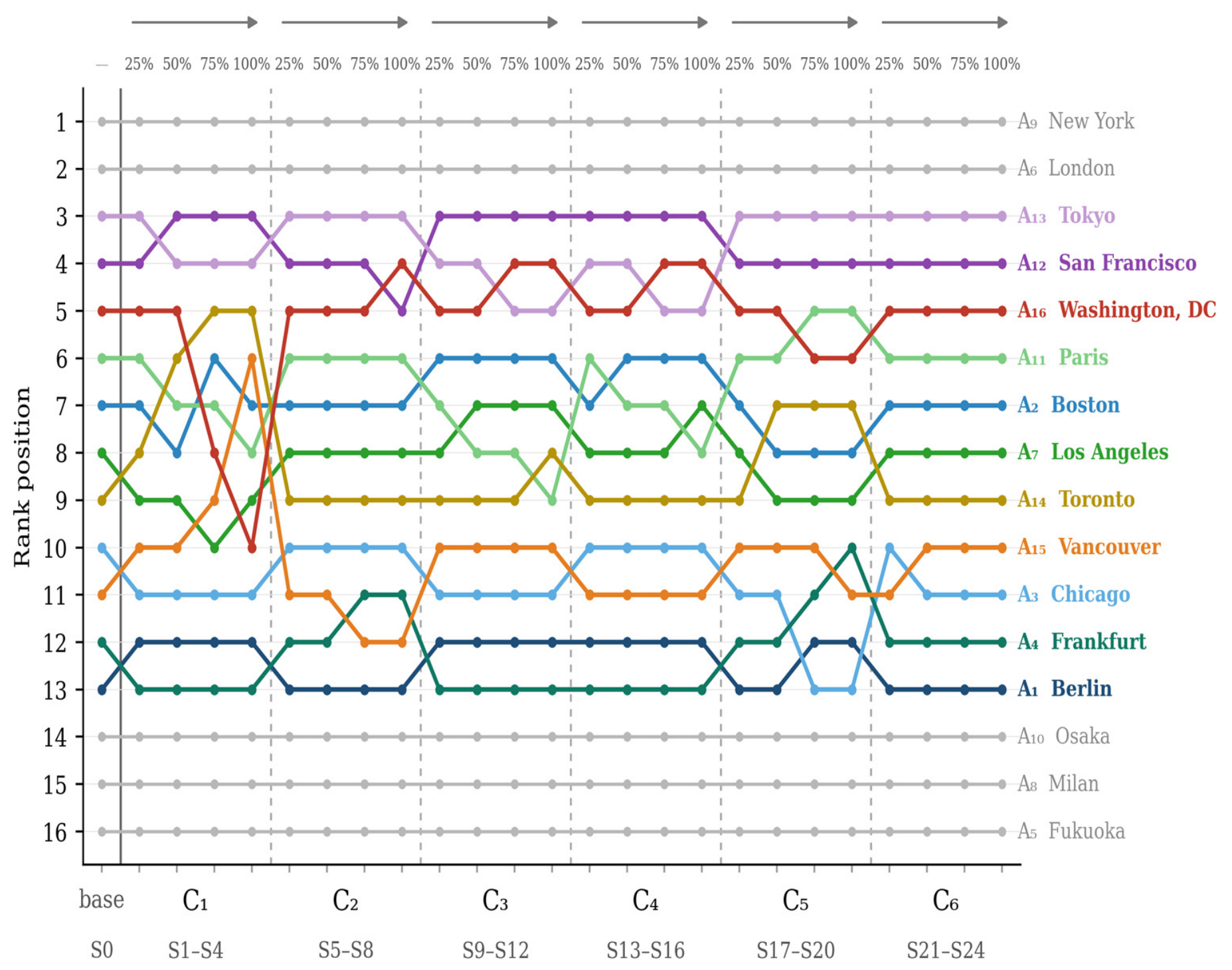
As a second step in the sensitivity analysis, the grey weights of the criteria are modified. In this context, the lower and upper limits of the grey weight for the first criterion ($C_1$) are reduced by the same proportion in four separate scenarios—at 25%, 50%, 75%, and 100%—and the reduced weight is distributed equally among the remaining five criteria in each scenario. The same procedure is repeated sequentially for the remaining five criteria, resulting in 24 scenarios (S1–S24). Because the grey weight of the criterion in question is zero in scenarios S4, S8, S12, S16, S20, and S24, those scenarios exclude this criterion from the assessment. Figure 5 illustrates that the 24 scenarios produce 19 separate ordering patterns. However, the SCCs between the initial ordering and the scenario-derived orderings range from 0.8882 to 1.0000, with an average correlation of 0.9819. The positions of $A_9$ and $A_6$, which have the highest performance, and $A_{10}$, $A_8$, and $A_5$, which have the lowest performance, remain unchanged across all scenarios. In contrast, $A_{16}$ shifts between the fourth and tenth ranks, while $A_{15}$ shifts between the sixth and 12th ranks, indicating that the movements are concentrated in the middle of the ranking.

5.3. Global Sensitivity Analysis

The sensitivity analyses in the previous two subsections vary the model’s parameters one at a time. Hence, these analyses do not account for combinations in which multiple parameters change simultaneously. For this reason, this subsection adds a global analysis. In each of 100,000 replications, the criterion weight vector is drawn from a flat Dirichlet distribution over the entire unit simplex so that every admissible weight vector is equally likely.

The whitenization coefficient in Equations (25)–(27) is drawn uniformly from the unit interval, and the aggregation-coefficient vector in Equation (28) from a flat Dirichlet distribution over its own simplex. The three aggregation coefficients weight the linear, vector, and non-linear normalization scores, respectively, so sampling them also lets the choice of normalization vary. Employing a single procedure corresponds to the vertices (1, 0, 0), (0, 1, 0) and (0, 0, 1); these are tested as separate scenarios in the aggregation-coefficient analysis of Section 5.1. Each replication employs a crisp weight vector rather than a grey one. The performance matrix in Table 10 is held fixed, and the whitenization coefficient carries its imprecision. The grey linguistic scale enters only via the weight bounds of Table 9, which this design discards. We vary it in the second run below. The replications employ a fixed random seed, and the standard error of any frequency presented below does not exceed 0.0016.

Table 17. Rank distributions under joint parameter sampling.

	Initial Rank	Mean Rank	90% Rank Interval	${\mathit{b}}^1$	${\mathit{b}}^{1-3}$
$A_9$ (New York)	1	1.41	1–3	0.738	0.974
$A_6$ (London)	2	2.03	1–3	0.230	0.971
$A_{13}$ (Tokyo)	3	5.20	2–11	0.000	0.480
$A_{12}$ (San Francisco)	4	4.14	2–8	0.032	0.462
$A_{16}$ (Washington)	5	6.54	3–13	0.000	0.064
$A_{11}$ (Paris)	6	7.43	4–12	0.000	0.002
$A_2$ (Boston)	7	7.88	4–14	0.000	0.010
$A_7$ (Los Angeles)	8	8.32	6–11	0.000	0.000
$A_{14}$ (Toronto)	9	7.05	4–10	0.000	0.009
$A_3$ (Chicago)	10	10.49	8–13	0.000	0.000
$A_{15}$ (Vancouver)	11	8.88	4–13	0.000	0.026
$A_4$ (Frankfurt)	12	11.07	6–13	0.000	0.000
$A_1$ (Berlin)	13	11.19	7–13	0.000	0.001
$A_{10}$ (Osaka)	14	13.90	12–15	0.000	0.000
$A_8$ (Milan)	15	14.81	12–16	0.000	0.000
$A_5$ (Fukuoka)	16	15.67	15–16	0.000	0.000

Notes: The mean rank and the 90% rank interval are calculated over the 100,000 replications. The interval runs from the 5th to the 95th percentile of the rank distribution. $b^1$ and $b^{1-3}$ are the rank acceptability indices of the first position and of the first three positions.

provides the resulting rank distributions, and

Table A9. Rank acceptability matrix from the joint parameter sampling (%).

	1	2	3	4	5	6	7	8	9	10	11	12	13	14	15	16
A9	73.8	17.5	6.2	1.0	0.7	0.4	0.2	0.1	0.1	0.1	<0.1	<0.1	–	–	–	–
A6	23.0	55.4	18.6	2.0	0.5	0.2	0.1	<0.1	0.1	<0.1	–	–	–	–	–	–
A13	<0.1	12.2	35.8	10.9	8.9	4.0	4.3	2.8	3.4	5.3	8.3	3.3	0.7	<0.1	–	–
A12	3.2	13.1	30.0	19.4	12.6	11.5	4.3	2.7	1.5	0.5	0.7	0.3	0.2	0.1	–	–
A16	–	1.0	5.4	21.9	22.7	11.4	9.0	7.4	4.9	4.0	2.6	2.9	2.4	2.1	1.6	0.7
A11	–	<0.1	0.2	19.7	10.3	17.5	7.6	8.6	7.0	10.3	9.2	6.5	3.0	<0.1	<0.1	–
A2	–	<0.1	1.0	9.2	14.9	11.9	16.8	14.0	7.8	4.5	4.6	4.8	3.4	2.1	3.9	1.0
A7	–	–	<0.1	0.3	3.0	14.6	15.8	22.1	19.5	13.6	6.8	2.6	1.5	0.2	<0.1	–
A14	–	0.1	0.8	8.9	17.7	13.8	18.2	14.5	11.9	10.2	3.3	0.4	0.1	–	–	–
A3	–	–	–	–	<0.1	0.1	2.8	5.4	18.6	25.2	21.7	14.3	10.5	1.1	0.3	<0.1
A15	–	0.6	2.0	5.8	5.4	7.8	11.3	10.4	10.5	9.6	20.1	9.0	4.3	2.0	1.1	<0.1
A4	–	–	<0.1	0.4	2.1	5.5	4.4	6.2	4.4	5.2	10.1	23.3	38.3	0.1	<0.1	–
A1	–	–	0.1	0.3	1.3	1.3	4.4	4.8	8.4	9.0	10.2	28.8	29.4	1.6	0.4	–
A10	–	–	–	–	–	–	0.1	0.2	0.8	1.2	1.6	2.9	4.2	74.2	14.9	–
A8	–	–	–	<0.1	<0.1	<0.1	0.7	0.8	1.0	1.3	0.8	1.0	1.8	13.6	50.7	28.3
A5	–	–	–	–	–	–	–	–	–	–	<0.1	<0.1	0.2	2.8	27.0	69.9

Notes: Cell $(i, r)$ reports the rank acceptability index $b^r$, that is, the percentage of the 100,000 replications of Section 5.3 in which alternative $i$ attains rank $r$. Rows follow the ranking of the G-MUNRA method. Each row and each column sums to 100. A dash $(-)$ marks a rank never attained, and “$<0.1$” a positive frequency that rounds to zero at one decimal place.

of Appendix D summarizes the complete rank acceptability matrix. The last two columns in Table 17 are rank acceptability indices in the sense of stochastic multi-criteria acceptability analysis (SMAA). Column $b^1$ is the first-rank index [45], whereas column $b^{1-3}$ sums the indices of the first three ranks, in line with SMAA-2 [46]. Since the measures relating to the criteria are not modelled stochastically, the central weight vectors and confidence factors for this framework are not reported. The indices function as a layer of robustness, not as a ranking tool. The Spearman correlation between the ranking of a replication and the ranking of the G-MUNRA method has a mean of 0.860. It is at least 0.90 in 49.3% of the replications and at least 0.594 in 95% of them. The obtained ordering shows a correlation of 0.977 with the average ranks in Table 17, so it is close to the ranking expected over the sampled parameter space. The first position is essentially limited to two cities: $A_9$ and $A_6$ account for 96.8% of all first ranks, with acceptabilities of 0.738 and 0.230. Apart from $A_{12}$ (0.032), no city attains it in more than one replication in a thousand. The three lowest positions are held by the same three cities in 86.9% of the replications. The third and fourth are contested: $A_{13}$ and $A_{12}$ enter the first three ranks in 48.0% and 46.2% of the replications. The middle of the ranking is far less determinate. The 90% intervals of the cities ranked fifth to 13th span six to 11 positions and overlap almost completely. None of them enters the first three ranks in more than 7% of the replications.

Next, we explore the grey linguistic scale in Table 2, first on its own. The three grey numbers are generalized to [0, $a$], [$a$, 1 − $a$] and [1 − $a$, 1], so that $a$ = 1/3 returns Table 2 itself. The scale degenerates as $a$ approaches 0 or 1/2, which bounds the scan range. The G-RANCOM-MUNRA model is repeated for sixty-one values of $a$ between 0.15 and 0.45. The criterion weights vary significantly, and the lower bound of $C_6$’s weight more than doubles over the interval. The ranking does not. Out of 61 calibrations, only two different rankings are obtained. The correlation with the reported ordering never drops below 0.9971, and no city shifts more than one position.

A second run of the same size restricts the weights to the grey bounds of Table 9. The calibration parameter $a$ of the grey linguistic scale is varied over [0.15, 0.45], so the bounds themselves move between replications, while the whitenization and aggregation coefficients continue to vary. Every uncertain element of the model is therefore perturbed simultaneously. The ranking is then almost fully identified. $A_9$ is ranked first and $A_6$ second in every replication, the three lowest positions are fixed, and the modal rank reproduces the reported position for all 16 city alternatives. The rank correlation averages 0.993 and never drops below 0.953.

The analyses above whiten the grey scores before ranking. The interval information can also be utilized directly to establish how firmly it supports each pairwise comparison. The grey aggregate score of a city is formulated before whitenization as the equally weighted sum of the three grey scores given in Equations (22)–(24).

For two grey numbers, the degree of possibility that $\otimes S_i$ is at least as large as $\otimes S_j$ is calculated as follows [39]:

$$P\left(\otimes S_i \ge \otimes S_j\right) = {\displaystyle \frac{max\left\{0, min\left(L_i + L_j, S_i^b - S_j^s\right)\right\}}{\left(L_i + L_j\right)}}$$

(29)

Here $L$ stands for the width of the corresponding interval. A value of 1 means full dominance, while 0.5 indicates indistinguishable intervals. None of the 120 ordered pairs implied by the reported ranking is reversed; the smallest value is 0.507, and 60 pairs are decided with a possibility of at least 0.90. Each of the five highest-ranked cities dominates each of the three lowest-ranked cities with a possibility of 1.000. Adjacent pairs are decided only marginally, with values between 0.51 and 0.76. The single exception is $A_9$ over $A_6$, decided with a possibility of 1.000.

Both analyses agree on where the framework discriminates and where it does not. Wide gaps are reliable. $A_9$ is far ahead of the other cities, and the highest-ranked cities are far ahead of the lowest-ranked cities under every source of uncertainty examined here, including the complete removal of expert weights. Narrow separations are not reliable. Adjacent pairs are distinguished only marginally, and after the weights are released, cities ranked fifth through 13th freely change positions. Consequently, G-MUNRA’s initial ranking supports comparisons among well-separated cities but not among cities in adjacent positions.

5.4. Validation of Results—Comparison with Existing Grey MCDM Approaches

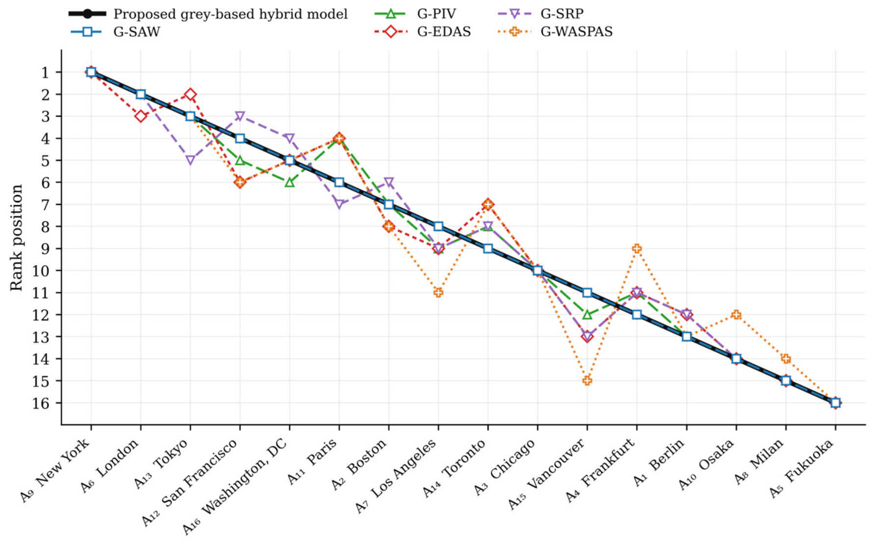
The comparative robustness analysis is conducted to assess the degree of consistency between the propounded grey-based decision-making methodology and several well-established grey MCDM approaches, namely G-EDAS [47], G-PIV [48], G-SAW [49], G-SRP [41], and G-WASPAS [50]. Figure 6 shows that the six ranking techniques produce five diverse rankings (see

Table A10. Scores and rankings of the five grey MCDM tools.

	G-SAW		G-PIV		G-EDAS		G-SRP		G-WASPAS
	Score	Rank	Score	Rank	Score	Rank	Score	Rank	Score	Rank
$A_1$	0.0656	13	0.2390	13	0.2714	12	6.0233	12	0.2604	13
$A_2$	0.0788	7	0.2132	7	0.3527	8	9.0021	6	0.3543	8
$A_3$	0.0718	10	0.2257	10	0.3360	10	7.0621	10	0.3292	10
$A_4$	0.0673	12	0.2299	11	0.3352	11	6.7159	11	0.3353	9
$A_5$	0.0444	16	0.2766	16	0.1349	16	2.0916	16	0.1393	16
$A_6$	0.1074	2	0.1439	2	0.6019	3	11.9760	2	0.6013	2
$A_7$	0.0778	8	0.2159	9	0.3473	9	7.5033	9	0.3195	11
$A_8$	0.0506	15	0.2637	15	0.1865	15	3.0372	15	0.1693	14
$A_9$	0.1407	1	0.0266	1	0.9309	1	12.6292	1	0.8347	1
$A_{10}$	0.0541	14	0.2539	14	0.2475	14	4.7922	14	0.2694	12
$A_{11}$	0.0842	6	0.1803	4	0.5344	4	8.7237	7	0.4893	4
$A_{12}$	0.0922	4	0.1877	5	0.4124	6	9.9429	3	0.3971	6
$A_{13}$	0.0961	3	0.1458	3	0.6037	2	9.2850	5	0.5611	3
$A_{14}$	0.0762	9	0.2146	8	0.3967	7	8.2361	8	0.3861	7
$A_{15}$	0.0691	11	0.2362	12	0.2605	13	5.5010	13	0.1425	15
$A_{16}$	0.0878	5	0.1886	6	0.4444	5	9.4801	4	0.4383	5

). However, in every method, $A_9$ ranks first, $A_3$ ranks tenth, and $A_5$ ranks 16th. The SCC between the introduced grey decision support algorithm and other grey ranking approaches ranges from 0.9235 to 1.0000, with an average of 0.9706. SCC values are 1.0000 for G-SAW, 0.9853 for G-PIV, 0.9765 for G-SRP, 0.9676 for G-EDAS, and 0.9235 for G-WASPAS. The deviations observed in G-PIV, G-SRP, and G-EDAS are limited to one or two positions, whereas the deviations in G-WASPAS range from one to four positions.

5.5. Validation of Results—Comparison with the Crisp and Fuzzy Methods

To further analyze the consistency and external validity of the introduced grey-based model, the initial ranking outputs are benchmarked against three comparison frameworks: a crisp RANCOM-MUNRA hybrid methodology, a fuzzy LBWA–ROV hybrid methodology, and a fuzzy LBWA–PIV hybrid methodology. By offering alternative approaches to decision information processing and uncertainty modelling, these comparison procedures enable testing the robustness of the developed grey approach across different MCDM paradigms.

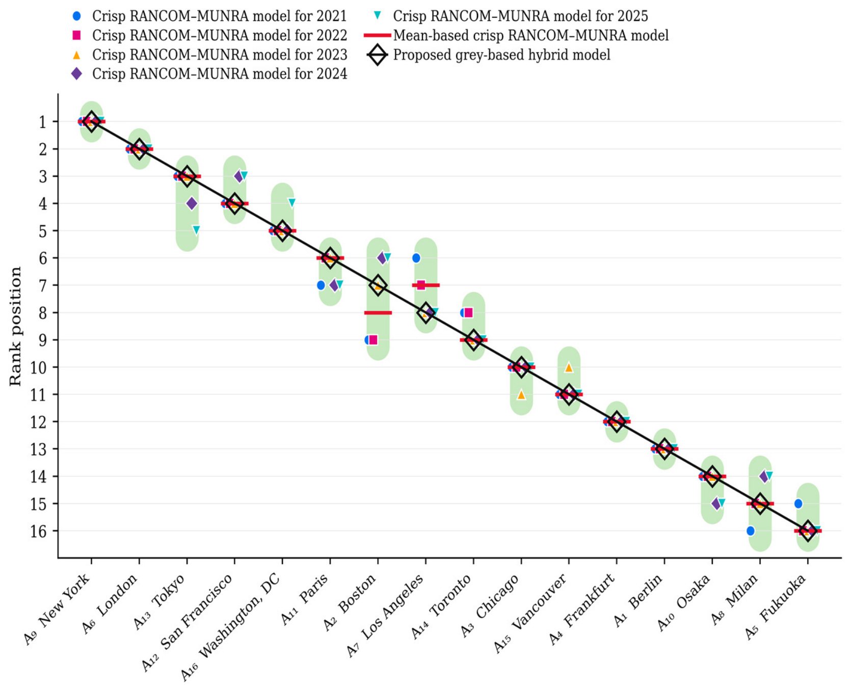
In the context of the application of the original (crisp) RANCOM-MUNRA hybrid methodology, a total of six models are designed based on annual data for the 2021–2025 period and average data for the same period. In the crisp-based models, the methodological steps of the RANCOM–MUNRA hybrid procedure are retained, and only the interval-valued inputs are replaced with point values. The results obtained from these models are illustrated in Figure 7. Figure 7 combines the rankings of the 16 city alternatives in the crisp-based models for each of the five years, the range of rankings for each alternative, and the rankings of the average-based crisp model and the introduced grey-based approach. Analysis of Figure 7 shows that all six crisp-based models closely match the grey-based model. The Spearman correlation coefficients range from 0.9824 to 0.9971 for the mean-based and annual models. In all crisp-based models, the number of positions showing complete overlap is between nine and 14. While the deviations remain within a narrow range, the rankings of the alternatives do not change by more than two positions. Additionally, alternatives $A_9$, $A_6$, $A_4$, and $A_1$ maintain their positions in all six models. However, $A_2$, the most volatile alternative, shifts between the 6th and 9th ranks over the five-year period.

Table A11. Scores and rankings of the crisp models.

	2021		2022		2023		2024		2025		Mean-Based
	Score	Rank	Score	Rank	Score	Rank	Score	Rank	Score	Rank	Score	Rank
$A_1$	0.2591	13	0.2648	13	0.2722	13	0.2588	13	0.2592	13	0.2658	13
$A_2$	0.3083	9	0.3166	9	0.3197	7	0.3715	6	0.3751	6	0.3409	8
$A_3$	0.2912	10	0.3014	10	0.2920	11	0.3123	10	0.3073	10	0.3038	10
$A_4$	0.2657	12	0.2787	12	0.2739	12	0.2742	12	0.2690	12	0.2743	12
$A_5$	0.1656	15	0.1881	16	0.1846	16	0.1400	16	0.1502	16	0.1656	16
$A_6$	0.4983	2	0.4849	2	0.4794	2	0.5175	2	0.4858	2	0.4968	2
$A_7$	0.3381	6	0.3346	7	0.3158	8	0.3470	8	0.3561	8	0.3422	7
$A_8$	0.1629	16	0.1895	15	0.1952	15	0.1984	14	0.2070	14	0.1908	15
$A_9$	0.7416	1	0.7460	1	0.7272	1	0.7486	1	0.7548	1	0.7489	1
$A_{10}$	0.1991	14	0.2133	14	0.2247	14	0.1955	15	0.1957	15	0.2062	14
$A_{11}$	0.3296	7	0.3662	6	0.3578	6	0.3593	7	0.3625	7	0.3570	6
$A_{12}$	0.4080	4	0.4079	4	0.4086	4	0.4536	3	0.4771	3	0.4330	4
$A_{13}$	0.4485	3	0.4460	3	0.4616	3	0.4328	4	0.3960	5	0.4383	3
$A_{14}$	0.3187	8	0.3332	8	0.3152	9	0.3244	9	0.3384	9	0.3299	9
$A_{15}$	0.2861	11	0.2928	11	0.2991	10	0.3056	11	0.2912	11	0.2994	11
$A_{16}$	0.4015	5	0.3960	5	0.3983	5	0.4176	5	0.4056	4	0.4075	5

in Appendix F reports the scores and rankings of the six crisp models.

Regarding the fuzzy-based methodologies, the Fuzzy Level-Based Weight Assessment (F-LBWA) [51], the Fuzzy Proximity Index Value (F-PIV) [52], and the Fuzzy Range of Value (F-ROV) [53] are utilized. In this context, the F-LBWA procedure calculates the criterion importance weights from a second round of expert evaluation, in which each expert assigned each criterion a level of importance and an intra-level importance value using the questionnaire reported in

Table A12. Questionnaire utilized in the second elicitation round (F-LBWA).

	Content
Goal	To obtain the level-based preference structure for the fuzzy benchmark models.
Material supplied	Definitions of the six GPCI-based criteria and the evaluation problem.
Step 1	Identify the criterion you consider the most important. This criterion defines the first significance level.
Step 2	Assign each remaining criterion to an importance level $\mathcal{l}$. Level 1 contains criteria whose importance is comparable to that of the most important criterion, level 2 contains criteria of lower importance, and so on.
Step 3	Within each level, express the relative importance of every criterion by an integer value $F$, where 0 denotes the most important criterion of that level and larger values denote lower importance.
Response format	One level index $\mathcal{l}$ and one importance value $F$ per criterion.

. In accordance with the F-LBWA procedure, the inter-expert values are first transformed into triangular fuzzy numbers. Next, the elasticity coefficient is assigned as $\xi = \mu + 1 = 4$ for each expert. Finally, the individual fuzzy weight vectors are aggregated by means of an unweighted Bonferroni mean operator with $p = q = 1$. For the F-PIV and F-ROV ranking process, the fuzzy decision matrix is built by representing each input as a triangular fuzzy number, with boundaries corresponding to the minimum and maximum annual observations and a peak at the five-year average. Thus, the grey and fuzzy matrices are based on exactly the same observations, and no linguistic scale or predefined membership function is utilized at any stage. The elicitation responses, the resulting fuzzy weights, and the outputs of the F-PIV and F-ROV procedures are reported in

Table A13. Second-round responses: level ℓ, importance value $F$ and the cross-expert fuzzy values.

	${\mathit{E}}_1$		${\mathit{E}}_2$		${\mathit{E}}_3$		${\mathit{E}}_4$		${\mathit{E}}_5$
	$\mathcal{l}$	$\mathit{F}$	$\mathcal{l}$	$\mathit{F}$	$\mathcal{l}$	$\mathit{F}$	$\mathcal{l}$	$\mathit{F}$	$\mathcal{l}$	$\mathit{F}$	(Min, Mean, Max) of $\mathit{F}$
$C_1$	1	0	1	0	1	1	1	0	1	2	(0.000, 0.600, 2.000)
$C_2$	3	1	3	2	1	2	1	1	1	2	(1.000, 1.600, 2.000)
$C_3$	2	1	2	1	1	0	1	2	2	1	(0.000, 1.000, 2.000)
$C_4$	2	3	2	2	2	1	2	2	2	2	(1.000, 2.000, 3.000)
$C_5$	2	3	2	3	2	2	2	1	1	0	(0.000, 1.800, 3.000)
$C_6$	3	2	3	1	2	2	2	2	2	3	(1.000, 2.000, 3.000)

,

Table A14. Individual and aggregated fuzzy criterion weights.

	${\mathit{E}}_1$	${\mathit{E}}_2$	${\mathit{E}}_3$	${\mathit{E}}_4$	${\mathit{E}}_5$	Aggregated ${\tilde{\mathit{w}}}_{\mathit{j}}$
$C_1$	(0.218, 0.322, 0.426)	(0.218, 0.322, 0.426)	(0.159, 0.242, 0.324)	(0.159, 0.242, 0.324)	(0.159, 0.247, 0.330)	(0.1821, 0.2743, 0.3650)
$C_2$	(0.093, 0.109, 0.131)	(0.093, 0.109, 0.131)	(0.159, 0.199, 0.259)	(0.159, 0.199, 0.259)	(0.159, 0.203, 0.264)	(0.1319, 0.1622, 0.2063)
$C_3$	(0.131, 0.164, 0.213)	(0.131, 0.164, 0.213)	(0.159, 0.223, 0.324)	(0.159, 0.223, 0.324)	(0.095, 0.126, 0.165)	(0.1345, 0.1792, 0.2455)
$C_4$	(0.119, 0.148, 0.189)	(0.119, 0.148, 0.189)	(0.087, 0.111, 0.144)	(0.087, 0.111, 0.144)	(0.087, 0.114, 0.147)	(0.0993, 0.1262, 0.1622)
$C_5$	(0.119, 0.151, 0.213)	(0.119, 0.151, 0.213)	(0.087, 0.114, 0.162)	(0.087, 0.114, 0.162)	(0.136, 0.196, 0.330)	(0.1091, 0.1443, 0.2137)
$C_6$	(0.087, 0.106, 0.131)	(0.087, 0.106, 0.131)	(0.087, 0.111, 0.144)	(0.087, 0.111, 0.144)	(0.087, 0.114, 0.147)	(0.0869, 0.1096, 0.1392)

and

Table A15. Fuzzy scores, defuzzified values and rankings obtained by F-PIV and F-ROV.

		F-PIV			F-ROV
		${\tilde{\mathit{S}}}_{\mathit{i}}$	${\mathit{S}}_{\mathit{i}}$	Rank	${\tilde{\mathit{\phi }}}_{\mathit{i}}$	${\mathit{\phi }}_{\mathit{i}}$	Rank
$A_1$	Berlin	(0.2855, 0.4057, 0.5958)	0.4173	13	(0.0942, 0.1462, 0.2358)	0.1588	12
$A_2$	Boston	(0.3251, 0.4698, 0.7151)	0.4866	8	(0.1206, 0.1863, 0.3057)	0.2042	7
$A_3$	Chicago	(0.3125, 0.4420, 0.6280)	0.4514	10	(0.1117, 0.1684, 0.2528)	0.1776	10
$A_4$	Frankfurt	(0.2948, 0.4265, 0.6030)	0.4340	12	(0.0951, 0.1518, 0.2288)	0.1586	13
$A_5$	Fukuoka	(0.1799, 0.2946, 0.4528)	0.3018	16	(0.0278, 0.0756, 0.1452)	0.0829	16
$A_6$	London	(0.4436, 0.6630, 0.9755)	0.6785	2	(0.1973, 0.3105, 0.4710)	0.3263	2
$A_7$	Los Angeles	(0.3348, 0.4782, 0.6832)	0.4885	7	(0.1240, 0.1895, 0.2855)	0.1997	8
$A_8$	Milan	(0.2072, 0.3274, 0.4866)	0.3339	15	(0.0374, 0.0898, 0.1588)	0.0953	15
$A_9$	New York	(0.5783, 0.8234, 1.1717)	0.8406	1	(0.2495, 0.3667, 0.5342)	0.3835	1
$A_{10}$	Osaka	(0.2239, 0.3527, 0.5288)	0.3606	14	(0.0532, 0.1082, 0.1858)	0.1157	14
$A_{11}$	Paris	(0.3436, 0.5158, 0.7577)	0.5274	6	(0.1203, 0.2036, 0.3228)	0.2156	6
$A_{12}$	San Francisco	(0.3707, 0.5641, 0.8653)	0.5821	4	(0.1477, 0.2432, 0.3972)	0.2627	3
$A_{13}$	Tokyo	(0.3883, 0.6044, 0.8918)	0.6163	3	(0.1453, 0.2489, 0.3883)	0.2608	4
$A_{14}$	Toronto	(0.3217, 0.4650, 0.6683)	0.4750	9	(0.1179, 0.1862, 0.2845)	0.1962	9
$A_{15}$	Vancouver	(0.2967, 0.4232, 0.6157)	0.4342	11	(0.1055, 0.1638, 0.2579)	0.1757	11
$A_{16}$	Washington, DC	(0.3779, 0.5475, 0.7823)	0.5583	5	(0.1481, 0.2270, 0.3395)	0.2382	5

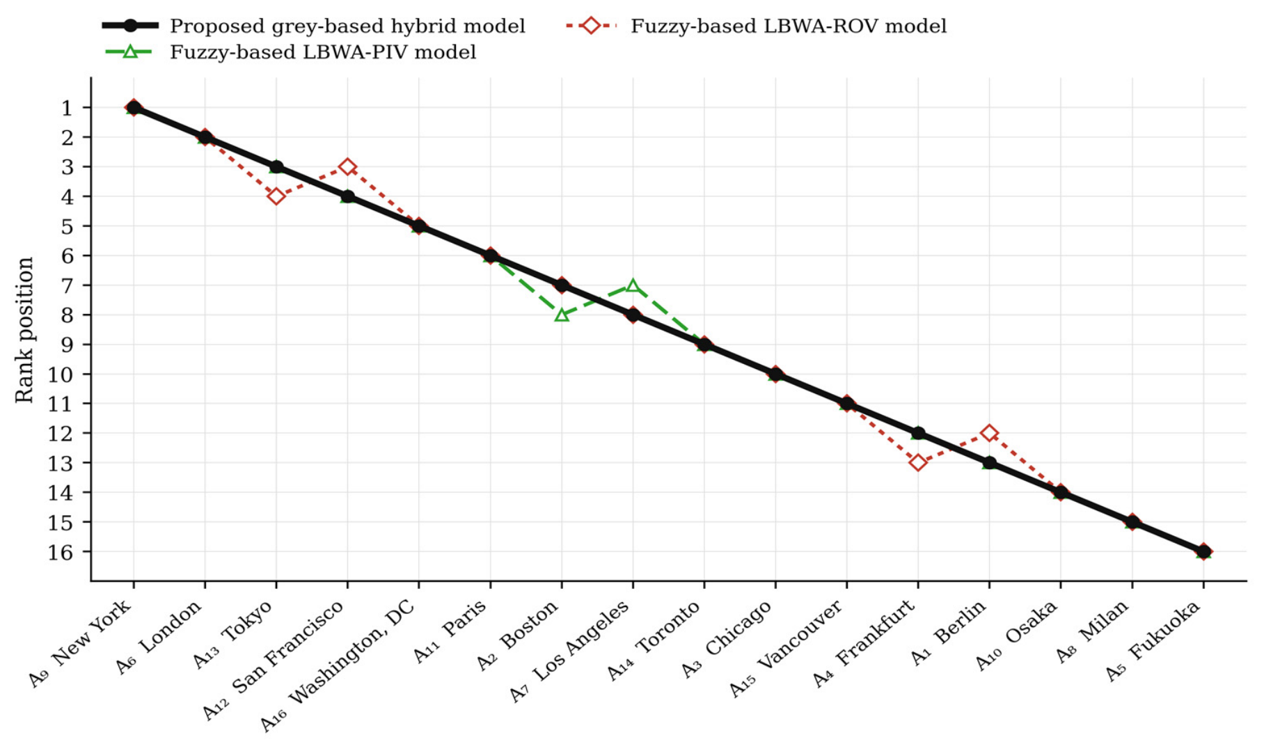
of Appendix G. The ranking results obtained by applying these procedures are displayed in Figure 8. According to Figure 8, when considering the ranking results of the three models, minor changes are observed in the positions of city alternatives such as $A_1$, $A_2$, $A_4$, $A_7$,$A_{12}$, and $A_{13}$. However, the remaining 10 city alternatives show no changes in position.

5.6. Validation of Results—Comparison with the Published GPCI Economy Rankings

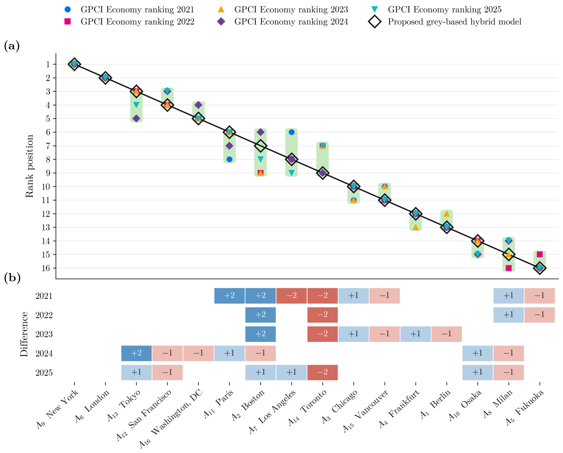
The final validity assessment compares the initial ranking with a benchmark derived independently of the proposed hybrid methodology. Given that the six criteria of this study constitute the indicators of the GPCI’s Economy function, the GPCI’s Economy function rankings for the 2021–2025 period (see

Table A16. Positions within the 16-city sample and comparison with the proposed model.

		2021	2022	2023	2024	2025	GPCI Range	Model Rank	Model Rank in Range
$A_9$	New York	1	1	1	1	1	1–1	1	Yes
$A_6$	London	2	2	2	2	2	2–2	2	Yes
$A_{13}$	Tokyo	3	3	3	5	4	3–5	3	Yes
$A_{12}$	San Francisco	4	4	4	3	3	3–4	4	Yes
$A_{16}$	Washington, DC	5	5	5	4	5	4–5	5	Yes
$A_{11}$	Paris	8	6	6	7	6	6–8	6	Yes
$A_2$	Boston	9	9	9	6	8	6–9	7	Yes
$A_7$	Los Angeles	6	8	8	8	9	6–9	8	Yes
$A_{14}$	Toronto	7	7	7	9	7	7–9	9	Yes
$A_3$	Chicago	11	10	11	10	10	10–11	10	Yes
$A_{15}$	Vancouver	10	11	10	11	11	10–11	11	Yes
$A_4$	Frankfurt	12	12	13	12	12	12–13	12	Yes
$A_1$	Berlin	13	13	12	13	13	12–13	13	Yes
$A_{10}$	Osaka	14	14	14	15	15	14–15	14	Yes
$A_8$	Milan	16	16	15	14	14	14–16	15	Yes
$A_5$	Fukuoka	15	15	16	16	16	15–16	16	Yes

of Appendix H) are compared separately with the hybrid model’s rankings. The results of these comparisons are displayed in Figure 9. Figure 9a indicates each city’s position in the five published rankings, the range that these positions cover, and the ranking assigned by the introduced hybrid model, while Figure 9b illustrates the variations between them. Figure 9a shows that each city’s position in the five published rankings falls within a band of no more than three ranks, and that the proposed hybrid model’s ranking falls within this band for all 16 city alternatives. Additionally, we compute an average correlation of 0.9818 between the rankings, confirming that the developed methodology’s rankings closely align with the published rankings.

6. Discussion, Theoretical Contributions, and Policy Implications

This manuscript proposes and applies a grey-based multi-criteria decision-support tool to compare the economic performance of major cities across G7 economies. Results from the G-RANCOM procedure indicate a differentiated importance structure among the economic criteria used in the assessment. The prominence of market size ($C_1$), economic vitality ($C_3$), and business environment ($C_5$) suggests that city-level economic performance in advanced economies is shaped primarily by structural and capacity-related factors, namely economic scale, financial and corporate depth, and the quality of the business ecosystem, including access to skilled labour. In contrast, market attractiveness ($C_2$) and ease of doing business ($C_6$) play a comparatively more limited role in distinguishing cities that operate within broadly similar institutional and regulatory contexts, such as those of the G7 economies.

This weight structure has two policy implications. The first concerns what does not differentiate cities within this group. Market attractiveness and ease of doing business, which capture growth momentum, economic freedom, corporate taxation, and country risk, rank fourth and sixth among the six criteria, and ease of doing business has the smallest weight in the set. This is not because such conditions are unimportant, but because G7 cities already operate under broadly similar institutional and regulatory regimes, so marginal adjustments in tax rates or regulatory burden have limited power to separate one city from another. The second implication concerns what differentiates them. Market size, economic vitality, and business environment jointly account for roughly two-thirds of the total weight, and all three describe accumulated capacity rather than current policy settings, which indicates that positions in this ranking respond to sustained investment in scale, financial and corporate depth, and labour-market quality rather than to short-term measures. One qualification applies to both implications. The weights express the relative importance that an expert panel attaches to each dimension rather than a causal estimate of its effect, so they indicate what informed observers regard as decisive, not what a city should expect to gain from acting on a given dimension.

The G-MUNRA algorithm places New York, London, and Tokyo in the top three positions. An examination of the criterion-level rankings shows these cities lead across several economic dimensions. New York ranks first in market size ($C_1$), economic vitality ($C_3$), and business environment ($C_5$), reflecting its economic scale, the depth of its financial markets, and its highly developed business ecosystem. London ranks first in human capital ($C_4$) and ease of doing business ($C_6$), which indicates its labour market capacity and the institutional conditions supporting economic activity. Tokyo, third overall, ranks second in economic vitality ($C_3$) and human capital ($C_4$) and third in market size ($C_1$), reflecting balanced performance across the most heavily weighted criteria. These patterns indicate that the leading cities owe their positions not to exceptional performance in a single dimension but to sustained, concurrent strength across several economically relevant criteria.

At the lower end of the ranking, Osaka, Milan, and Fukuoka occupy the last three positions, and the criterion-level pattern behind these positions is the inverse of the pattern observed at the top. Fukuoka is last of the sixteen cities in market size ($C_1$) and business environment ($C_5$), the criteria ranked first and third by weight, and 15th in economic vitality ($C_3$), which carries the second-largest weight. Milan is last in market attractiveness ($C_2$) and ease of doing business ($C_6$) and 14th in business environment ($C_5$), and its only mid-table position, sixth in human capital ($C_4$), belongs to one of the two least influential criteria. Osaka is the 15th in business environment ($C_5$), 14th in market attractiveness ($C_2$), and 13th in ease of doing business ($C_6$), and its comparatively better standing in economic vitality ($C_3$) is not sufficient to compensate for them. Low overall positions in this framework therefore arise from simultaneous weakness in the heavily weighted structural criteria rather than from a single deficient indicator.

The global sensitivity analysis reported in Section 5.3 qualifies these findings. The separation of New York from the remaining alternatives, and that of the highest-ranked from the lowest-ranked cities, remains stable over the entire admissible parameter space, whereas alternatives occupying adjacent positions are separated only marginally. Comparative statements about cities in adjacent positions should therefore be avoided.

The findings of this study offer theoretical implications for both the MCDM literature and the economic assessment of cities. First, the results confirm that urban economic performance is inherently multi-dimensional and cannot be adequately captured through single-indicator or composite-index approaches. The observed rankings indicate that high-performing cities achieve their positions through consistently strong performance across multiple economic criteria rather than dominance in a single dimension, reinforcing a central premise of MCDM theory: overall performance emerges from the joint contribution of interrelated criteria. Second, the study contributes methodologically to decision science by extending RANCOM and MUNRA to the interval grey-number domain. To the best of the authors’ knowledge, these formulations are the first adaptations of RANCOM and MUNRA in which both criterion weighting and alternative ranking use interval-valued information. By embedding grey numbers in both stages of the decision process, the proposed framework extends these methods to environments characterized by data imprecision and variability while preserving their original computational structure. Third, in contrast to the predominantly country-level focus of existing economic performance studies, the study introduces a city-level multi-criteria evaluation framework and provides a systematic MCDM-based comparison of economic performance across major global cities.

The findings also offer insights for urban policymakers and economic strategists in advanced economies. The ranking results indicate that improvements in urban economic performance are unlikely to be achieved through isolated or single-indicator interventions, and that cities benefit from policy approaches addressing several economic dimensions in a coordinated and mutually reinforcing manner. For cities at the lower end of the performance distribution, the results indicate that gradual and balanced progress across several dimensions is more likely to produce durable improvement than an attempt to raise performance rapidly in a single area.

In practical terms, a city administration can apply the framework in four steps. First, the city’s interval scores in Table 10 are compared with those of the reference group to identify the criteria on which even the upper bound falls below the sample median, distinguishing a structural shortfall from a temporary one. Second, each shortfall is weighted by the corresponding criterion weight in Table 9, which orders candidate interventions by the ranking movement that closing them would produce rather than by their political visibility. Third, the implied movement is compared with the rank acceptability indices in Table A9, and where it does not exceed the uncertainty of the current position, the intervention should be justified on grounds other than benchmarking. Fourth, the exercise is repeated as new editions of the index appear, and the width of a city’s intervals is monitored in its own right, since a widening interval signals instability in the underlying position even when the midpoint is unchanged. Applied this way, the framework functions less as a league table than as a diagnostic instrument that shows where a city’s position is weak, how much a given improvement would matter, and whether the resulting movement can be distinguished from measurement uncertainty.

7. Limitations and Future Research

The proposed grey-based framework is based on seven assumptions. Each is stated below together with the risk it carries for the reported ranking, the evidence that bounds its influence, and the extension that would relax it.

The bounds of each grey number are the minimum and the maximum of five annual observations, so interval width is governed by extreme years rather than by measurement error, and the whitened scores of cities with volatile histories are correspondingly less determinate. The rank acceptability indices in Section 5.3 limit this impact to the middle of the ranking, and intervals constructed from longer series or from percentile-trimmed bounds would mitigate it further.

Before ranking the alternatives, each interval is reduced to a single value, which presents cities with overlapping intervals in a definitive order. The degrees of possibility in Section 5.3 indicate that no ordered pair implied by the reported ordering is reversed and that adjacent pairs are decided only marginally, and reporting the results in interval-dominance form throughout would remove the need for whitenization.

The criterion weights come from a five-member panel whose importance coefficients the authors assigned. Thus, a different panel or a different assignment rule could yield a different weight vector. The concordance reported in Section 4.5.1 and the 10 expert-team scenarios in Section 5.1 keep every city within one position of its reported rank, and a larger panel would allow these coefficients to be estimated rather than assigned.

The criterion set is confined to the GPCI Economy function. Therefore, research and development, accessibility, environment, cultural interaction, and livability dimensions are excluded, and the findings describe economic performance rather than overall urban performance. The scope is stated explicitly in Section 1, and the external comparison in Section 5.6 is against the Economy ranking rather than the overall index; extending the indicator system beyond the economic dimension would broaden the conceptual scope.

The study sample consists of the G7 cities covered by the index, a group that is institutionally homogeneous, which limits the transferability of the weight structure to emerging and developing economies. The rule in Section 4.4 makes the sample exhaustive rather than selective within the G7, and applying the model to cities outside this group would directly test transferability.

The aggregation is additive and therefore assumes preferential independence, under which conceptually related criteria may compensate for one another. The diagnostics in Section 4.6 report a maximum absolute correlation of 0.767 and a maximum variance inflation factor of 7.25, both below conventional thresholds, and a Choquet integral or an outranking model would be required in settings where interaction is documented.

All performance data come from a single source and enter the model after the index’s standardization and reverse-scoring procedures. Hence, any bias in those procedures propagates to the ranking. Appendix A presents the orientation and transformation of each sub-indicator, and replicating the analysis with an independent indicator system would allow assessment of source dependence.

8. Conclusions

This study developed an integrated grey-based multi-criteria approach to benchmark urban economic performance under uncertainty and applied it to 16 G7 cities included in the Global Power City Index. Criterion importance was calculated using a grey extension of RANCOM, which converts the ordinal evaluations of a five-member expert committee into interval weights, and cities were ranked using a grey extension of MUNRA, which combines linear, vector, and non-linear normalization.

Two key findings emerge from the analysis. Market size, economic vitality, and the business environment account for approximately two-thirds of the total criterion weight. This suggests that the economic ranking among G7 cities is driven more by accumulated structural capacity than by financial and regulatory conditions, which are already similar across these cities. In the ranking, New York, London, and Tokyo occupy the top three positions, while Osaka, Milan, and Fukuoka occupy the bottom three. This is the result of strengths or weaknesses observed simultaneously across multiple highly weighted criteria, rather than performance in a single dimension in each case.

We analyzed the stability of these positions at three levels. Scenario analyses of the expert-team composition, the whitenization coefficient, the aggregation coefficients, and the criterion weights yield rank correlations between 0.89 and 1.00, and the two highest and three lowest positions remain unchanged under the expert-panel and criterion-weight scenarios. A global analysis of 100,000 replications, in which all model parameters vary jointly over their admissible ranges, assigns New York the first position in 74% of the replications and leaves the three lowest positions unchanged in 87%, whereas cities in adjacent positions are separated only marginally. Comparison with five established grey methods, with crisp and fuzzy counterparts, and with the published GPCI Economy rankings yields Spearman correlations between 0.92 and 1.00. The framework therefore supports comparisons between well-separated cities rather than between cities in neighbouring positions.

This work’s methodological contribution is the formulation of RANCOM and MUNRA in an interval grey environment, allowing criterion weighting and alternative ranking with interval-valued information while preserving the computational structure of the original methods. For urban policymakers, the framework provides a diagnostic tool rather than a league table, since it identifies the criteria on which a city’s position is structurally weak, orders candidate interventions by the ranking movement they would produce, and indicates whether that movement can be distinguished from measurement uncertainty. The assumptions on which these results rest, and the evidence bounding their influence, are set out in Section 7.