Mean-Square Bounded Synchronization for Complex Networks Under Cyber-Attack via Hybrid Self-Triggered Impulsive Control

Abstract

The issue of mean-square bounded synchronization for complex networks subject to random disturbances, time-varying delays, and cyber-attacks is investigated in this paper. We employ static and dynamic self-triggered impulsive control strategies, which can predict the next impulsive instant based on the current state of the system. These strategies not only ensure the convergence of the control error but also reduce the number of triggering instants. Denial-of-service (DoS) and deception attacks are jointly modeled using two independent Bernoulli stochastic processes. Meanwhile, sufficient conditions for the mean-square bounded synchronization are established through the Lyapunov functional method. In addition, it is demonstrated that these control strategies rule out Zeno behavior, ensuring the reliable achievement of mean-square bounded synchronization. Finally, the accuracy of the theoretical analysis is illustrated through numerical examples. Compared to static triggering, the dynamic self-triggered impulsive control mechanism demonstrates superior performance in reducing the number of triggers, as shown by experimental results.

1. Introduction

Networks composed of abundant nodes (or vertices) joined by a highly complex set of interwoven edges are known as complex networks (CNs) [1]. Because of their characteristics, such as structural complexity, dynamic evolution, diverse connectivity patterns, and nonlinear dynamical behaviors, CNs have attracted extensive attention and research efforts from a large number of scholars [2,3]. The application domains of CNs in real life are extensive, including power systems, transportation networks, biological systems, and financial networks [4,5,6,7,8]. However, the existence of time delays in network systems leads to data loss and increased communication congestion, which negatively impact the real-time capability and stability of CNs [9,10,11,12,13,14,15]. Thus, random disturbances are regarded as non-negligible factors in the behavior of CNs, and the investigation of stochastic CNs with time delays is considered to have important practical significance [16,17,18,19].

Synchronization behavior in CNs is categorized under the domain of network dynamical behavior. The classification includes bounded synchronization, exponential synchronization, bipartite synchronization, and asymptotic synchronization, reflecting different convergence behaviors in network dynamics [5,6]. Additionally, bounded synchronization has emerged as a significant area of research [20,21,22]. It ensures that the system states converge within a certain bound while achieving state consistency and system stability [23,24,25]. Compared with exponential synchronization, which emphasizes fast convergence, bounded synchronization focuses more on synchronization performance under constraints, thereby avoiding resource waste and excessive system burdens caused by aggressive control actions. Hence, bounded synchronization carries substantial theoretical and practical meaning in networked systems research [26,27,28,29]. Recently, significant research achievements have been made in the study of bounded synchronization within CNs. In [23], based on a unified strategy, Zhu et al. investigated the bounded synchronization problem of heterogeneous complex dynamical networks by developing a joint-diagonalization-like technique. In [28], Wang et al. investigated the global bounded synchronization of complex dynamical networks based on Lyapunov function methods and graph theory. Zhang et al. [30] designed a dual-channel stochastic deception attack scheme and proposed an adaptive secure impulsive consensus strategy to investigate the mean-square consensus problem for time-varying nonlinear multi-agent systems. Wu et al. [31] investigated the mean-square bounded synchronization of fractional-order chaotic Lur’e systems under deception attack using an impulsive control approach.

In order to achieve bounded synchronization, one may adopt control methods including event-triggered control, impulsive control, self-triggered impulsive control, and adaptive event-triggered impulsive control. There is universal agreement that in event-triggered control, events are generated based on a predefined triggering condition [32,33]. Nevertheless, the requirement of continuous input of the control signal into the system results in resource inefficiency [34,35]. Under impulsive control, dynamic systems experience instantaneous state changes at discrete times, which result in lower control costs [36]. Additionally, self-triggered impulsive control predicts the upcoming impulsive moment according to the current state of the system, avoiding continuous monitoring and thus contributing to energy savings [17,37,38]. Due to the advantages of self-triggered impulsive control, it has attracted increasing research interest from scholars. Wang et al. [39] investigated Lyapunov stability of nonlinear systems using discrete-time self-triggered impulsive control and derived sufficient conditions for Zeno-free behavior and global asymptotic stability. Xie et al. [40] proposed a self-triggered delayed impulsive control scheme to investigate group consensus of multi-agent systems. Importantly, the self-triggered impulsive control strategy ensures that Zeno behavior is effectively excluded. Zeno behavior is an undesirable phenomenon characterized by the emergence of infinitely many events in a finite period. When triggering occurs too frequently, it can cause system instability and significantly increase the consumption of computing and communication resources. Owing to characteristics such as intrinsic time delays, constraints on periodic execution, and deliberate algorithmic design, self-triggered impulsive control inherently rules out the possibility of continuous triggering within a finite time interval [38]. Consequently, the occurrence of Zeno phenomena is effectively ruled out, guaranteeing both system stability and optimal use of resources.

Furthermore, the achievement of bounded synchronization under self-triggered impulsive control is affected by cyber-attacks. Common attack types include DoS attacks, deception attacks, and replay attacks [41,42,43,44,45]. Obviously, DoS attacks and deception attacks are the most prevalent. DoS attacks disrupt normal system operation by interfering with or blocking the system’s communication channels [44]. Deception attacks occur when adversaries inject fabricated or altered data into the system, deceiving the controller into treating malicious inputs as genuine, ultimately resulting in erroneous control decisions [46,47]. The essence of deception attacks, unlike deception attacks, lies in compromising the integrity and genuineness of data, which, in turn, adversely affects the stability of the CN. Recently, researchers have been increasingly investigating the issue of synchronization for CNs under cyber-attack. In [41], Liu et al. investigated the design of pinning observers to realize secure and reliable synchronization in complex dynamical networks under DoS attack. In [46], Liu et al. explored how nonlinear coupling and deception attacks affect the mean-square exponential stability of systems by using a sampled-data control strategy and a generalized Halanay inequality. In [48], Wang et al. used distributed controllers and parameter estimators to study the stability of distributed control systems under replay attack. Since both the timing and the type of attacks are unpredictable, attackers can flexibly choose attack types to enhance their effectiveness. Simultaneously, modeling both attack types in a unified framework in CNs studies is more representative of real-world scenarios. Therefore, how self-triggered impulsive control can achieve bounded synchronization in CNs subject to DoS and deception attacks is a challenging problem.

Prompted by the preceding analysis, we devoted this study to investigating the problem of mean-square bounded synchronization of CNs under cyber-attack by self-triggered impulsive control, and we prove in this paper that the Zeno phenomenon is avoided via this control mechanism. Although self-triggered impulsive control, DoS attacks, and deception attacks have each been investigated separately in the existing literature, their theoretical integration is nontrivial. Existing studies mainly focus on event-triggered control, single attack scenarios, or exponential synchronization. In contrast, the present work establishes a unified analytical framework for mean-square bounded synchronization of stochastic complex networks subject to simultaneous DoS and deception attacks via hybrid self-triggered impulsive control. The coexistence of random cyber-attacks and self-triggered impulsive mechanisms introduces additional stochastic jump terms into the Lyapunov analysis, which cannot be handled directly using existing stability results [13,49,50,51,52]. Therefore, new sufficient synchronization criteria and trigger conditions are developed in this paper. The key contributions are summarized below:

(1)

A unified theoretical framework is established for the mean-square bounded synchronization of stochastic complex networks subject to simultaneous DoS and deception attacks using hybrid self-triggered impulsive control. Compared with existing studies focusing on a single attack or event-triggered strategy, the proposed framework allows the synchronization problem to be analyzed under the condition of multiple random cyber-attacks within one Lyapunov-based analytical framework.

(2)

DoS and deception attacks are jointly modeled using two independent Bernoulli stochastic sequences within a unified framework, making it possible to fully identify potential security risks and improve the overall system resilience.

This paper is structured as follows. Section 2 introduces the model, controller, and assumptions and defines mean-square bounded synchronization. Section 3 designs static and dynamic self-triggered impulsive control schemes. The main theoretical results are presented in Section 4. The simulation outcomes and their implications are exhibited in Section 5. Finally, Section 6 provides a summary of this paper.

2. Preliminaries and Model Description

Notation: To begin, it is essential to introduce some mathematical symbols. ${\mathbb{R}}^n$ represents the n-dimensional Euclidean space. Additionally, ${\mathbb{R}}^{+}$ stands for $[0,+\infty )$. $x^{\mathrm{T}}$ and $\parallel x\parallel$ denote the transpose of x for $x\in {\mathbb{R}}^n$ and the Euclidean norm, respectively. Let $L=\{0,1,\dots ,\}$, $L_1=\{1,2,\dots ,m\}$, $L_2=\{1,2,\dots ,M\}$, $L_3=\{0,1,2,\dots ,M\}$. Furthermore, given a complete probability space $(\Omega ,\mathcal{F},\mathbb{F},\mathbb{P})$ equipped with a filtration ${\left\{{\mathcal{F}}_t\right\}}_{t\ge t_0}$ that satisfies usual conditions, and let $\mathbb{E}(·)$ be the mathematical expectation. Let $\mathcal{P}\mathcal{C}([-\tau ,0];{\mathbb{R}}^n)$ denote the family of continuous functions $g:[-\tau ,0]\to {\mathbb{R}}^n$ with norm $\parallel g\parallel =\sup \left\{\right|g\left(\eta \right)|:-\tau \le \eta \le 0\}$. $L_{{\mathcal{F}}_0}^2([-\tau ,0];{\mathbb{R}}^{n\times n})$ means the family of all ${\mathcal{F}}_0$-measurable $\mathcal{P}\mathcal{C}([-\tau ,0];{\mathbb{R}}^{n\times n})$-valued random variables with ${\mathbb{E}\parallel g\parallel }^2\le \infty$ for all $g=\left\{g\right(\eta ):-\tau \le \eta \le 0\}$. Moreover, consider a strongly connected digraph $\mathcal{D}$ whose edge weights are characterized by the matrix $\mathcal{U}={\left(a_{sv}\right)}_{m\times m}$.

We consider the drive system model as follows:

$$\begin{array}{cc}\hfill \mathrm{d}{d}_s\left(t\right)=& [l_s(d_s\left(t\right),d_s(t-{\tau }_0\left(t\right)),t)\hfill \\ \hfill & +{\displaystyle \sum _{i1=1}^M}{\Psi }_{i1}\left(t\right){\displaystyle \sum _{v=1}^m}{f}_{sv}^{\left(i1\right)}{\Pi }_{sv}^{\left(i1\right)}(d_s(t-{\tau }_{i1}\left(t\right)),d_v(t-{\tau }_{i1}\left(t\right)),t)]\mathrm{d}t\hfill \\ \hfill & +W_s(d_s\left(t\right),d_s(t-{\tau }_0\left(t\right)),t)\mathrm{d}\omega \left(t\right),s\in L_1,\hfill \end{array}$$

(1)

where $d_s\left(t\right)\in {\mathbb{R}}^n$ is the state vector associated with the s-node, while $l_s(·),W_s(·)$: ${\mathbb{R}}^n\times {\mathbb{R}}^n\times {\mathbb{R}}^{+}\to {\mathbb{R}}^n$ are continuous functions. ${\Pi }_{sv}^{\left(i1\right)}(·)$: ${\mathbb{R}}^n\times {\mathbb{R}}^n\times {\mathbb{R}}^{+}\to {\mathbb{R}}^n$ stands for the non-linear coupling function, ${\Psi }_{i1}\left(t\right)$ characterizes the dynamic variation of the coupling strength, and $f_{sv}^{\left(i1\right)}\in \{0,1\}$ determines whether a link exists between any two nodes in the $i1$-th subnetwork. There is no directed edge from node s to node v in the $i1$-th subnetwork if and only if $f_{sv}^{\left(i1\right)}=0$, and the converse is also true. $\omega \left(t\right)$ is a continuous-time stochastic process representing one-dimensional scalar Brownian motion defined on the given complete probability space $(\Omega ,\mathcal{F},\mathbb{F},\mathbb{P})$. Moreover, ${\tau }_0$ represents the internal time delay. ${\tau }_{i1}\left(t\right)$ is the time-varying delay in the coupling between nodes, whose characteristics are determined by the structure of the $i1$-th subnetwork.

Consider the following response system, which corresponds to system (1):

$$\begin{array}{cc}\hfill \mathrm{d}{r}_s\left(t\right)=& [l_s(r_s\left(t\right),r_s(t-{\tau }_0\left(t\right)),t)+u_s\left(t\right)\hfill \\ \hfill & +{\displaystyle \sum _{i1=1}^M}{\Psi }_{i1}\left(t\right){\displaystyle \sum _{v=1}^m}{f}_{sv}^{\left(i1\right)}{\Pi }_{sv}^{\left(i1\right)}(r_s(t-{\tau }_{i1}\left(t\right)),r_v(t-{\tau }_{i1}\left(t\right)),t)]\mathrm{d}t\hfill \\ \hfill & +W_s(r_s\left(t\right),r_s(t-{\tau }_0\left(t\right)),t)\mathrm{d}\omega \left(t\right),s\in L_1,\hfill \end{array}$$

(2)

where $r_s\left(t\right)\in {\mathbb{R}}^n$ is the state vector associated with the s-th node and $u_s\left(t\right)$ is the control input.

We introduce the synchronization error vector as ${\Xi }_s\left(t\right)=r_s\left(t\right)-d_s\left(t\right)$, and the corresponding error system takes the form

$$\begin{array}{cc}\hfill \mathrm{d}{\Xi }_s\left(t\right)=& [{\tilde{l}}_s({\Xi }_s\left(t\right),{\Xi }_s(t-{\tau }_0\left(t\right)),t)+u_s\left(t\right)\hfill \\ \hfill & +{\displaystyle \sum _{i1=1}^M}{\Psi }_{i1}\left(t\right){\displaystyle \sum _{v=1}^m}{f}_{sv}^{\left(i1\right)}{\tilde{\Pi }}_{sv}^{\left(i1\right)}({\Xi }_s(t-{\tau }_{i1}\left(t\right)),{\Xi }_v(t-{\tau }_{i1}\left(t\right)),t)]\mathrm{d}t\hfill \\ \hfill & +{\tilde{W}}_s({\Xi }_s\left(t\right),{\Xi }_s(t-{\tau }_0\left(t\right)),t)\mathrm{d}\omega \left(t\right),s\in L_1,\hfill \end{array}$$

(3)

where

$$\begin{array}{cc}\hfill & {\tilde{l}}_s({\Xi }_s\left(t\right),{\Xi }_s(t-{\tau }_0\left(t\right)),t)=l_s(r_s\left(t\right),r_s(t-{\tau }_0\left(t\right)),t)-l_s(d_s\left(t\right),d_s(t-{\tau }_0\left(t\right)),t),\hfill \\ \hfill & {\tilde{W}}_s({\Xi }_s\left(t\right),{\Xi }_s(t-{\tau }_0\left(t\right)),t)=W_s(r_s\left(t\right),r_s(t-{\tau }_0\left(t\right)),t)-W_s(d_s\left(t\right),d_s(t-{\tau }_0\left(t\right)),t),\hfill \\ \hfill & {\tilde{\Pi }}_{sv}^{\left(i1\right)}({\Xi }_s(t-{\tau }_{i1}\left(t\right)),{\Xi }_v(t-{\tau }_{i1}\left(t\right)),t)={\Pi }_{sv}^{\left(i1\right)}(r_s(t-{\tau }_{i1}\left(t\right)),r_v(t-{\tau }_{i1}\left(t\right)),t)\hfill \\ \hfill & -{\Pi }_{sv}^{\left(i1\right)}(d_s(t-{\tau }_{i1}\left(t\right)),d_v(t-{\tau }_{i1}\left(t\right)),t).\hfill \end{array}$$

To achieve for systems (1) and (2) the mean-square bounded synchronization under cyber-attack via self-triggered impulsive control, the impulsive control is created as

$$\begin{array}{c}\hfill u_s\left(t\right)={\displaystyle \sum _{j=1}^{\infty }}\left\{(1-\varpi \left(t\right))T_{s,j}[{\Xi }_s\left(t\right)+\kappa \left(t\right)B_s\left(t\right)]\right\}\delta (t-{\zeta }_{s,j}),\end{array}$$

(4)

in which $T_{s,j}$ is the impulsive gain; $B_s\left(t\right)$ represents the deception signal; $\delta (·)$ stands for the Dirac function; $\left\{{\zeta }_{s,j}\right\}$ is the self-triggered impulsive sequence of the s-th node, which is defined as $0={\zeta }_{s,0}<{\zeta }_{s,1}<\cdots <{\zeta }_{s,j}<\cdots$; and $\varpi \left(t\right)$ and $\kappa \left(t\right)$ are random variable that obey the Bernoulli distribution and satisfy

$$\begin{array}{cc}\hfill & P\left\{\varpi \right(t)=0\}=\varpi ,P\left\{\varpi \right(t)=1\}=1-\varpi ,\hfill \\ \hfill & P\left\{\kappa \right(t)=0\}=\kappa ,P\left\{\kappa \right(t)=1\}=1-\kappa ,\hfill \end{array}$$

in which $\varpi ,\kappa \in (0,1]$.

For controller (4) subject to random cyber-attacks, we can classify the attacks into three cases:

• Case 1: $\varpi \left(t\right)=1$ indicates that a DoS attack is in effect,

  $$\begin{array}{c}\hfill u_s\left(t\right)=0;\end{array}$$
• Case 2: $\varpi \left(t\right)=0$ and $\kappa \left(t\right)=1$ indicate that a deception attack is occurring,

  $$\begin{array}{c}\hfill u_s\left(t\right)={\displaystyle \sum _{j=1}^{\infty }}{T}_{s,j}[{\Xi }_s\left(t\right)+B_s\left(t\right)]\delta (t-{\zeta }_{s,j});\end{array}$$
• Case 3: $\varpi \left(t\right)=0$ and $\kappa \left(t\right)=0$ represent an attack-free situation,

  $$\begin{array}{c}\hfill u_s\left(t\right)={\displaystyle \sum _{j=1}^{\infty }}{T}_{s,j}{\Xi }_s\left(t\right)\delta (t-{\zeta }_{s,j}).\end{array}$$

According to the foregoing analysis, the error system is expressed as

$$\begin{array}{c}\hfill \left\{\begin{array}{cc}\hfill \mathrm{d}{\Xi }_s\left(t\right)=& [{\tilde{l}}_s({\Xi }_s\left(t\right),{\Xi }_s(t-{\tau }_0\left(t\right)),t)\hfill \\ \hfill & +{\displaystyle \sum _{i1=1}^M}{\Psi }_{i1}\left(t\right){\displaystyle \sum _{v=1}^m}{f}_{sv}^{\left(i1\right)}{\tilde{\Pi }}_{sv}^{\left(i1\right)}({\Xi }_s(t-{\tau }_{i1}\left(t\right)),{\Xi }_v(t-{\tau }_{i1}\left(t\right)),t)]\mathrm{d}t\hfill \\ \hfill & +{\tilde{W}}_s({\Xi }_s\left(t\right),{\Xi }_s(t-{\tau }_0\left(t\right)),t)\mathrm{d}\omega \left(t\right),\hfill \\ \hfill \Delta {\Xi }_s\left({\zeta }_{s,j}\right)=& {\Xi }_s\left({\zeta }_{s,j}\right)-{\Xi }_s\left({\zeta }_{s,j}^{-}\right)=(1-\varpi \left({\zeta }_{s,j}\right))T_{s,j}[{\Xi }_s\left({\zeta }_{s,j}^{-}\right)+\kappa \left({\zeta }_{s,j}\right)B_s\left({\zeta }_{s,j}\right)],\hfill \end{array}\right.\end{array}$$

(5)

where $\Delta {\Xi }_s\left({\zeta }_{s,j}\right)={\Xi }_s\left({\zeta }_{s,j}^{+}\right)-{\Xi }_s\left({\zeta }_{s,j}^{-}\right)$, ${\Xi }_s\left({\zeta }_{s,j}^{+}\right)={\Xi }_s\left({\zeta }_{s,j}\right)$.

Remark 1.

In this paper, DoS attacks and deception attacks are modeled by two independent Bernoulli stochastic processes for analytical convenience and mathematical tractability. Such a probabilistic model has been extensively employed in the literature on networked control systems to describe randomly occurring cyber-attacks when only statistical occurrence information is available. Under this assumption, explicit synchronization conditions can be established via Lyapunov functional analysis. Nevertheless, we acknowledge that real cyber-attacks may present bursty, correlated, or Markovian characteristics, which cannot be fully captured by independent Bernoulli variables. Therefore, the adopted attack model should be regarded as an idealized approximation, while extension to more realistic attack models remains an interesting direction for future research.

Assumption 1.

For all $i1\in L_2$, $0<{\Psi }_{i1}\left(t\right)\le {\Psi }_{i1}$ holds for a positive constant ${\Psi }_{i1}$ and all t.

Assumption 2.

There are positive constants ${\tau }_{i1}$, ${\tau }_0$, τ, such that for any $i1\in L_3$, the time-varying delay parameters ${\tau }_{i1}\left(t\right)$ and ${\tau }_0\left(t\right)$ satisfy

$$\begin{array}{c}\hfill 0\le {\tau }_{i1}\left(t\right)\le {\tau }_{i1}\le \tau ,0\le {\tau }_0\left(t\right)\le {\tau }_0\le \tau .\end{array}$$

Assumption 3.

For each $s\in L_1$, $\exists {\alpha }_s^{\left(1\right)},{\alpha }_s^{\left(2\right)},{\alpha }_s^{\left(3\right)},{\alpha }_s^{\left(4\right)},K_{sv}^{\left(i1\right)}>0$ such that $\forall d_s,{\widehat{d}}_s,r_s,{\widehat{r}}_s\in {\mathbb{R}}^n$, the inequalities below hold:

$$\begin{array}{cc}\hfill & \parallel l_s(r_s,{\widehat{r}}_s,t)-l_s(d_s,{\widehat{d}}_s,t){\parallel }^2\le {\alpha }_s^{\left(1\right)}\parallel r_s-d_s{\parallel }^2+{\alpha }_s^{\left(2\right)}{\parallel {\widehat{r}}_s-{\widehat{d}}_s\parallel }^2,\hfill \\ \hfill & \parallel W_s(r_s,{\widehat{r}}_s,t)-W_s(d_s,{\widehat{d}}_s,t){\parallel }^2\le {\alpha }_s^{\left(3\right)}\parallel r_s-d_s{\parallel }^2+{\alpha }_s^{\left(4\right)}{\parallel {\widehat{r}}_s-{\widehat{d}}_s\parallel }^2,\hfill \\ \hfill & \parallel {\Pi }_{sv}^{\left(i1\right)}(r_s,r_v,t)-{\Pi }_{sv}^{i1}(d_s,d_v,t){\parallel }^2\le K_{sv}^{\left(i1\right)}(\parallel r_s-d_s{\parallel }^2+\parallel r_v-d_v{\parallel }^2).\hfill \end{array}$$

Assumption 4.

If $B_s\left(t\right)$ is the deception signal, then $\exists b>0$ such that $\parallel B_s{\left(t\right)\parallel }^2\le b$ for each $s\in L_1$.

Definition 1.

The drive system (1) and the response system (2) are said to achieve mean-square bounded synchronization if there exists a constant $ϵ>0$ such that

$$\begin{array}{c}\hfill \underset{t\to \infty }{lim}\sup \mathbb{E}{\parallel \Xi \left(t\right)\parallel }^2\le ϵ,\end{array}$$

where $\Xi \left(t\right)={({\Xi }_1^T\left(t\right),{\Xi }_2^T\left(t\right),\cdots ,{\Xi }_m^T\left(t\right))}^T\in {\mathbb{R}}^{mn}$.

3. Design of Static and Dynamic Trigger Mechanisms

A static self-triggered impulsive update mechanism is suggested, in which the impulsive instant for the s-th node is given by

$$\begin{array}{c}\hfill {\zeta }_{s,j+1}=\inf \{t>{\zeta }_{s,j}|Z_s\left(t\right)>0\},\end{array}$$

(6)

where $Z_s\left(t\right)=\parallel {\Delta }_s\left({\zeta }_{s,j}\right){\parallel }^2(e^{{\beta }_1(t-{\zeta }_{s,j})}-1)-\mu {\parallel {\Delta }_s\left({\zeta }_{s,j}\right)\parallel }^2-{\rho }_1{e}^{{\beta }_2(t-t_0)}-{\displaystyle \frac{{\rho }_2}{{(t-t_0)}^2}}$, ${\Delta }_s\left(t\right)=(1-\varpi \left({\zeta }_{s,j}\right))[{\Xi }_s\left({\zeta }_{s,j}^{-}\right)+\kappa \left({\zeta }_{s,j}\right)B_s\left({\zeta }_{s,j}\right)]$, $0<\mu <1$. ${\rho }_1,{\rho }_2,{\beta }_1,{\beta }_2$ are positive constants.

Furthermore, to address the interference of some uncontrollable factors, we also design a dynamic self-triggered impulsive mechanism with a float function $h_s\left(t\right)$ that better meets actual needs:

$$\begin{array}{c}\hfill {\zeta }_{s,j+1}=\inf \{t>{\zeta }_{s,j}|Z_s\left(t\right)-\omega \chi h_s\left(t\right)-\omega \phi \left(j\right)>0\},\end{array}$$

(7)

in which $\omega ,\chi >0$, $h_s\left(t\right)>0$. Furthermore, $h_s\left(t_0\right)$ is the initial value of $h_s\left(t\right)$. Assume that

$$\begin{array}{c}\hfill {\dot{h}}_s\left(t\right)=-\chi h_s\left(t\right)+\phi \left(j\right),\end{array}$$

(8)

in which $\phi \left(j\right)>0$ stands for the floating boundary of $h_s\left(t\right)$ at the j-th impulsive instant. The boundary sequence ${\left\{\phi \left(j\right)\right\}}_j^{+\infty }$ is decreasing.

Remark 2.

The parameters $\omega >0$ and $\chi >0$ are design constants. The parameter ω determines the weight of the dynamic threshold in the triggering condition, whereas χ determines the decay rate of the internal dynamic variable $h_s\left(t\right)$. A larger dynamic-threshold term generally postpones the triggering instant and reduces the triggering frequency, while the prescribed maximum inter-triggering interval $I_2$ should still be satisfied. The sequence $\left\{\phi \right(j\left)\right\}$ is selected as a positive monotonically decreasing sequence. For $t\in [{\zeta }_{s,j},{\zeta }_{s,j+1})$, the solution of (8) is

$$\begin{array}{c}\hfill h_s\left(t\right)=e^{-\chi (t-{\zeta }_{s,j})}{h}_s\left({\zeta }_{s,j}\right)+{\displaystyle \frac{\phi \left(j\right)}{\chi }}(1-e^{-\chi (t-{\zeta }_{s,j})}).\end{array}$$

Therefore, if $h_s\left(t_0\right)>0$, $\chi >0$, and $\phi \left(j\right)>0$, then $h_s\left(t\right)>0$ for all $t\ge t_0$.

Remark 3.

Consecutive DoS attacks may prevent the impulsive input from being successfully implemented and may also cause the triggering set in (6) or (7) to be empty. In this case, the locally implemented backup scheduling rule introduced in Remark 5 is activated to maintain the triggering sequence.

Remark 4.

Self-triggered impulsive control computes the next impulsive instant in advance at the current triggering instant by using the sampled state information and system parameters. This approach not only avoids persistent state observation but also prevents excessive impulse activations, significantly reducing the resource demands imposed on the controller. However, reference [53] uses a dynamic event-triggered control mechanism. The controller update is determined by pre-defined trigger conditions and requires continuous monitoring of the system state, which increases resource consumption. The work in [54] proposes an adaptive event-triggered impulsive control method that relies on continuous observation of the system state to evaluate a predefined event condition. By adjusting the triggering threshold using the adaptive parameter $a_i^{\left(m\right)}$ and the dynamic variable ${\gamma }_i\left(t\right)$, a low triggering frequency can be maintained even under varying system dynamics, resulting in relatively low computational resource consumption—though at the cost of certain monitoring overhead. In contrast to event-triggered and adaptive-triggered approaches, self-triggering mechanisms exhibit broader application potential by avoiding continuous monitoring, enabling prior computation of the next trigger time, and offering simplicity in implementation.

Remark 5.

A successful DoS attack at the impulsive instant ${\zeta }_{s,j}$ may lead to ${\Delta }_s\left({\zeta }_{s,j}\right)=0$, in which case the triggering set in (6) or (7) may be empty. To ensure that the triggering sequence remains well defined, a locally implemented backup interval $I_b>0$ is introduced. If the triggering set in (6) or (7) is empty, the next triggering instant is scheduled as

$$\begin{array}{c}\hfill {\zeta }_{s,j+1}={\zeta }_{s,j}+I_b.\end{array}$$

The backup interval is selected such that $I_1<I_b<I_2$, where $I_1$ and $I_2$ are the lower and upper bounds of the inter-impulse intervals used in Theorems 1 and 2. Since this backup scheduling procedure is implemented locally, it is independent of whether the impulsive control input is successfully transmitted. Therefore, consecutive DoS attacks may prevent the impulsive input from being executed, but they do not interrupt the generation of subsequent triggering instants.

Lemma 1.

The dynamic self-triggering mechanism generates fewer triggering events than the static self-triggering mechanism. Denote the $(j+1)$-th triggering instant as ${\zeta }_{s,j+1}^1$ and ${\zeta }_{s,j+1}^2$ for the static and dynamic cases, respectively. Then, it follows that ${\zeta }_{s,j+1}^1\le {\zeta }_{s,j+1}^2$.

Proof. 

Consider the inter-impulse intervals $[{\zeta }_{s,j}^1,{\zeta }_{s,j+1}^1)$ and $[{\zeta }_{s,j}^2,{\zeta }_{s,j+1}^2)$ for static and dynamic self-triggered impulsive control, respectively. Assume ${\zeta }_{s,j}^1={\zeta }_{s,j}^2$, and suppose, for contradiction, that ${\zeta }_{s,j+1}^1>{\zeta }_{s,j+1}^2$. Then, combining (6) and (7), we deduce that at time ${\zeta }_{s,j+1}^2$, no trigger occurs under the static mechanism, whereas the dynamic mechanism triggers an instant. Hence, we have

$$\begin{array}{c}\hfill \parallel {\Delta }_s\left({\zeta }_{s,j}\right){\parallel }^2(e^{{\beta }_1({\zeta }_{s,j+1}^2-{\zeta }_{s,j})}-1)-\mu {\parallel {\Delta }_s\left({\zeta }_{s,j}\right)\parallel }^2-{\rho }_1{e}^{{\beta }_2({\zeta }_{s,j+1}^2-t_0)}-{\displaystyle \frac{{\rho }_2}{{({\zeta }_{s,j+1}^2-t_0)}^2}}<0,\end{array}$$

but

$$\begin{array}{cc}\hfill & \parallel {\Delta }_s\left({\zeta }_{s,j}\right){\parallel }^2(e^{{\beta }_1({\zeta }_{s,j+1}^2-{\zeta }_{s,j})}-1)-\mu {\parallel {\Delta }_s\left({\zeta }_{s,j}\right)\parallel }^2\hfill \\ \hfill & -{\rho }_1{e}^{{\beta }_2({\zeta }_{s,j+1}^2-t_0)}-{\displaystyle \frac{{\rho }_2}{{({\zeta }_{s,j+1}-t_0)}^2}}>\omega \chi h_s\left({\zeta }_{s,j+1}\right)+\omega \phi \left(j\right)>0,\hfill \end{array}$$

which is a contradiction. If ${\Delta }_s\left({\zeta }_{s,j}\right)=0$, the triggering sets in both (6) and (7) are empty. According to Remark 5, the static and dynamic mechanisms employ the same backup interval $I_b$, and hence

$$\begin{array}{c}\hfill {\zeta }_{s,j+1}^1={\zeta }_{s,j+1}^2={\zeta }_{s,j}+I_b.\end{array}$$

Therefore, ${\zeta }_{s,j+1}^1\le {\zeta }_{s,j+1}^2$ also holds in this special case. □

4. Main Results

In this section, we establish sufficient conditions for the mean-square bounded synchronization of systems (1) and (2) based on a Lyapunov functional construction. Furthermore, Zeno behavior can be excluded under cyber-attack via hybrid self-triggered impulsive control.

Theorem 1.

Suppose that Assumptions 1–4 are valid and that system (5) satisfies the following requirements:

$$\begin{array}{cc}\hfill & {\theta }_{sv}={\max }_{1\le i1\le M}\left\{{\Psi }_{i1}{f}_{sv}^{\left(i1\right)}{K}_{sv}^{\left(i1\right)}\right\},\hfill \\ \hfill & a_1={\max }_{1\le s\le m}\{1+{\alpha }_s^{\left(1\right)}+{\alpha }_s^{\left(3\right)}+{\displaystyle \sum _{i1=1}^M}{\displaystyle \sum _{v=1}^m}{\Psi }_{i1}{f}_{sv}^{\left(i1\right)}\},\hfill \\ \hfill & a_2={\max }_{1\le s\le m}\{{\alpha }_s^{\left(2\right)}+{\alpha }_s^{\left(4\right)}\},\hfill \\ \hfill & a_3={\max }_{1\le s\le m}\left\{{\displaystyle \sum _{i1=1}^M}{\displaystyle \sum _{v=1}^m}({\Psi }_{i1}{f}_{sv}^{\left(i1\right)}{K}_{sv}^{\left(i1\right)}+{\theta }_{sv})\right\},\hfill \\ \hfill & {\sigma }_1={\max }_{1\le s\le m}\{1+\varpi T_{s,j}^2+2\varpi T_{s,j}+\varpi (1-\kappa )T_{s,j}^2+\varpi (1-\kappa )\},\hfill \\ \hfill & {\widehat{\sigma }}_2={\max }_{1\le s\le m}\left\{3\varpi (1-\kappa )T_{s,j}^{2}b\right\},\hfill \\ \hfill & \mathbb{E}\left\{(1-\varpi \left({\zeta }_{s,j}\right))\right\}=\varpi ,\mathbb{E}\left\{{(1-\varpi \left({\zeta }_{s,j}\right))}^2\right\}=\varpi ,\hfill \\ \hfill & \mathbb{E}\left\{(1-\varpi \left({\zeta }_{s,j}\right))\kappa \left({\zeta }_{s,j}\right)\right\}=\varpi (1-\kappa ),\mathbb{E}\left\{{(1-\varpi \left({\zeta }_{s,j}\right))}^2{\kappa }^2\left({\zeta }_{s,j}\right)\right\}=\varpi (1-\kappa ),\hfill \\ \hfill & {\displaystyle \frac{\ln {\sigma }_1}{I_2}}+a<0,0<I_1<{\zeta }_{s,j+1}-{\zeta }_{s,j}<I_2,\varrho =I_2-I_1,0<\mu <1.\hfill \end{array}$$

Under these conditions, system (5) can realize mean-square bounded synchronization and avoid Zeno behavior when subject to cyber-attacks by using static self-triggered impulsive control.

Proof. 

To be clearer and more intuitive, this proof consists of two steps.

• Step 1: Define the Lyapunov functional as

  $$Y(\Xi (t),t)={\displaystyle \sum _{s=1}^m}{\Lambda }_s{Y}_s({\Xi }_s\left(t\right),t),$$

  where $Y_s({\Xi }_s\left(t\right),t)={\parallel {\Xi }_s\left(t\right)\parallel }^2$, ${\Lambda }_s\in {\mathbb{R}}_{+}$ refers to the cofactor of the s-th diagonal element of the Laplacian matrix of the strongly connected digraph $(\mathcal{D},\mathcal{U})$.

When $t\in [{\zeta }_{s,j-1},{\zeta }_{s,j})$, the differential operator for $Y(\Xi (t),t)$ is expressed as

$$\begin{array}{c}\hfill \mathcal{L}Y(\Xi \left(t\right),t)={\displaystyle \sum _{s=1}^m}{\Lambda }_s\mathcal{L}{Y}_s({\Xi }_s\left(t\right),t),\end{array}$$

(9)

in which

$$\begin{array}{cc}\hfill \mathcal{L}{Y}_s({\Xi }_s\left(t\right),t)=& 2{\Xi }_s^{\mathrm{T}}\left(t\right)[{\tilde{l}}_s({\Xi }_s\left(t\right),{\Xi }_s(t-{\tau }_0\left(t\right)),t)\hfill \\ \hfill & +{\displaystyle \sum _{i1=1}^M}{\Psi }_{i1}\left(t\right){\displaystyle \sum _{v=1}^m}{f}_{sv}^{\left(i1\right)}{\tilde{\Pi }}_{sv}^{\left(i1\right)}({\Xi }_s(t-{\tau }_{i1}\left(t\right)),{\Xi }_v(t-{\tau }_{i1}\left(t\right)),t)]\hfill \\ \hfill & +\parallel {\tilde{W}}_s({\Xi }_s\left(t\right),{\Xi }_s(t-{\tau }_0\left(t\right)),t){\parallel }^2,\hfill \end{array}$$

(10)

according to Assumption 3, we can easily obtain

$$\begin{array}{c}\hfill 2{\Xi }_s^{\mathrm{T}}\left(t\right){\tilde{l}}_s({\Xi }_s\left(t\right),{\Xi }_s(t-\tau \left(t_0\right)),t)\le (1+{\alpha }_s^{\left(1\right)})\parallel {\Xi }_s\left(t\right){\parallel }^2+{\alpha }_s^{\left(2\right)}{\parallel {\Xi }_s(t-{\tau }_0\left(t\right))\parallel }^2,\end{array}$$

(11)

$$\begin{array}{c}\hfill \parallel {\tilde{W}}_s({\Xi }_s,{\Xi }_s(t-{\tau }_0\left(t\right)),t){\parallel }^2\le {\alpha }_s^{\left(3\right)}\parallel {\Xi }_s{\left(t\right)\parallel }^2+{\alpha }_s^{\left(4\right)}{\parallel {\Xi }_s(t-{\tau }_0\left(t\right))\parallel }^2,\end{array}$$

(12)

and

$$\begin{array}{cc}\hfill & 2{\Xi }_s^{\mathrm{T}}\left(t\right){\displaystyle \sum _{i1=1}^M}{\Psi }_{i1}\left(t\right){\displaystyle \sum _{v=1}^m}{f}_{sv}^{\left(i1\right)}{\tilde{\Pi }}_{sv}^{\left(i1\right)}({\Xi }_s(t-{\tau }_{i1}\left(t\right)),{\Xi }_v(t-{\tau }_{i1}\left(t\right)),t)\hfill \\ \hfill \le & {\displaystyle \sum _{i1=1}^M}{\displaystyle \sum _{v=1}^m}{\Psi }_{i1}{f}_{sv}^{\left(i1\right)}(\parallel {\Xi }_s{\left(t\right)\parallel }^2+K_{sv}^{\left(i1\right)}(\parallel {\Xi }_s(t-{\tau }_{i1}\left(t\right)){\parallel }^2+\parallel {\Xi }_v(t-{\tau }_{i1}\left(t\right)){\parallel }^2\left)\right)\hfill \\ \hfill \le & {\displaystyle \sum _{i1=1}^M}{\displaystyle \sum _{v=1}^m}[{\Psi }_{i1}{f}_{sv}^{\left(i1\right)}\parallel {\Xi }_s{\left(t\right)\parallel }^2+({\Psi }_{i1}{f}_{sv}^{\left(i1\right)}{K}_{sv}^{\left(i1\right)}+{\theta }_{sv}){\parallel {\Xi }_s(t-{\tau }_{i1}\left(t\right))\parallel }^2\hfill \\ \hfill & +{\theta }_{sv}(\parallel {\Xi }_v(t-{\tau }_{i1}\left(t\right)){\parallel }^2-\parallel {\Xi }_s(t-{\tau }_{i1}\left(t\right)){\parallel }^2\left)\right].\hfill \end{array}$$

(13)

By substituting (11)–(13) into (9), we can obtain the following inequality:

$$\begin{array}{cc}\hfill \mathcal{L}Y(\Xi (t),t)\le & {\displaystyle \sum _{s=1}^m}{\Lambda }_s(1+{\alpha }_s^{\left(1\right)}+{\alpha }_s^{\left(3\right)}+{\displaystyle \sum _{i1=1}^M}{\displaystyle \sum _{v=1}^m}{\Psi }_{i1}{f}_{sv}^{\left(i1\right)}){\parallel {\Xi }_s\left(t\right)\parallel }^2\hfill \\ \hfill & +{\displaystyle \sum _{s=1}^m}{\Lambda }_s({\alpha }_s^{\left(2\right)}+{\alpha }_s^{\left(4\right)}){\parallel {\Xi }_s(t-{\tau }_0\left(t\right))\parallel }^2\hfill \\ \hfill & +{\displaystyle \sum _{s=1}^m}{\Lambda }_s{\displaystyle \sum _{i1=1}^M}{\displaystyle \sum _{v=1}^m}({\Psi }_{i1}{f}_{sv}^{\left(i1\right)}{K}_{sv}^{\left(i1\right)}+{\theta }_{sv}){\parallel {\Xi }_s(t-{\tau }_{i1})\parallel }^2\hfill \\ \hfill & +{\displaystyle \sum _{s=1}^m}{\displaystyle \sum _{i1=1}^M}{\displaystyle \sum _{v=1}^m}{\Lambda }_s{\theta }_{sv}(\parallel {\Xi }_v(t-{\tau }_{i1}\left(t\right)){\parallel }^2-\parallel {\Xi }_s(t-{\tau }_{i1}\left(t\right)){\parallel }^2).\hfill \end{array}$$

(14)

Based on Theorem 2.2 in [55], it holds that

$$\begin{array}{c}\hfill {\displaystyle \sum _{s,v=1}^m}{\Lambda }_s{\theta }_{sv}{F}_{sv}({\Xi }_s,{\Xi }_v)=\sum _{Q\in \mathbb{Q}}\overline{W}\left(Q\right)\sum _{(q,p)\in {\rm Y}\left(C_Q\right)}{F}_{pq}({\Xi }_p,{\Xi }_q),\end{array}$$

where $F_{sv}({\Xi }_s,{\Xi }_v)$ represents arbitrary function, $\mathbb{Q}$ is the set of all spanning unicyclic graphs Q of $(\mathcal{D},\mathcal{U})$, $C_Q$ is the directed cycle of Q and $\overline{W}\left(Q\right)$ stands for the weight of Q.

Then, we have

$$\begin{array}{c}\hfill {\displaystyle \sum _{s=1}^m}{\displaystyle \sum _{v=1}^m}{\Lambda }_s{\theta }_{sv}\left[\parallel {\Xi }_v(t-{\tau }_{i1}\left(t\right)){\parallel }^2-{\parallel {\Xi }_s(t-{\tau }_{i1}\left(t\right))\parallel }^2\right]=0.\end{array}$$

(15)

Substituting (15) into (14), we arrive at the following inequality

$$\begin{array}{cc}\hfill \mathcal{L}Y(\Xi (t),t)\le & {\displaystyle \sum _{s=1}^m}{\Lambda }_s(1+{\alpha }_s^{\left(1\right)}+{\alpha }_s^{\left(3\right)}+{\displaystyle \sum _{i1=1}^M}{\displaystyle \sum _{v=1}^m}{\Psi }_{i1}{f}_{sv}^{\left(i1\right)}){\parallel {\Xi }_s\left(t\right)\parallel }^2\hfill \\ \hfill & +{\displaystyle \sum _{s=1}^m}{\Lambda }_s({\alpha }_s^{\left(2\right)}+{\alpha }_s^{\left(4\right)}){\parallel {\Xi }_s(t-{\tau }_0\left(t\right))\parallel }^2\hfill \\ \hfill & +{\displaystyle \sum _{s=1}^m}{\Lambda }_s{\displaystyle \sum _{i1=1}^M}{\displaystyle \sum _{v=1}^m}({\Psi }_{i1}{f}_{sv}^{\left(i1\right)}{K}_{sv}^{\left(i1\right)}+{\theta }_{sv}){\parallel {\Xi }_s(t-{\tau }_{i1})\parallel }^2.\hfill \end{array}$$

(16)

Furthermore, we can calculate that

$$\begin{array}{cc}\hfill \mathcal{L}Y(\Xi (t),t)\le & a_1{\displaystyle \sum _{s=1}^m}{\Lambda }_s\parallel {\Xi }_s{\left(t\right)\parallel }^2+a_2{\displaystyle \sum _{s=1}^m}{\Lambda }_s{\parallel {\Xi }_s(t-{\tau }_0\left(t\right))\parallel }^2\hfill \\ \hfill & +a_3{\displaystyle \sum _{s=1}^m}{\Lambda }_s{\parallel {\Xi }_s(t-{\tau }_{i1}\left(t\right))\parallel }^2.\hfill \end{array}$$

(17)

We have

$$\begin{array}{c}\hfill \mathcal{L}Y(\Xi \left(t\right),t)\le (a_1+a_2{q}_1+a_3{q}_2)Y(\Xi \left(t\right),t),\end{array}$$

in which $q_1,q_2>1$.

Hence, it gives

$$\begin{array}{c}\hfill \mathcal{L}Y(\Xi (t),t)\le aY(\Xi (t),t),\end{array}$$

(18)

in which $a=a_1+a_2{q}_1+a_3{q}_2$. Subsequently, we have

$$\begin{array}{c}\hfill \mathbb{E}\mathcal{L}Y(\Xi \left(t\right),t)\le a\mathbb{E}Y(\Xi \left(t\right),t),\forall t\in [{\zeta }_{s,j-1},{\zeta }_{s,j}).\end{array}$$

(19)

We can obtain

$$\begin{array}{c}\hfill \mathbb{E}Y(\Xi \left(t\right),t)\le e^{a(t-{\zeta }_{s,j-1})}\mathbb{E}Y(\Xi \left({\zeta }_{s,j-1}\right),{\zeta }_{s,j-1}).\end{array}$$

(20)

When $t={\zeta }_{s,j}$, we can calculate the mean value for the $Y(\Xi (t),t)$ as follows:

$$\begin{array}{c}\hfill \mathbb{E}Y(\Xi \left(t\right),t)={\displaystyle \sum _{s=1}^m}{\Lambda }_s\mathbb{E}{Y}_s({\Xi }_s\left({\zeta }_{s,j}\right),{\zeta }_{s,j}),\end{array}$$

(21)

in which

$$\begin{array}{cc}\hfill & \mathbb{E}{Y}_s({\Xi }_s\left({\zeta }_{s,j}\right),{\zeta }_{s,j})\hfill \\ \hfill =& \mathbb{E}\parallel {\Xi }_s\left({\zeta }_{s,j}\right){\parallel }^2\hfill \\ \hfill =& \mathbb{E}\left\{{[{\Xi }_s\left({\zeta }_{s,j}^{-}\right)+(1-\varpi \left({\zeta }_{s,j}\right))T_{s,j}({\Xi }_s\left({\zeta }_{s,j}^{-}\right)+\kappa \left({\zeta }_{s,j}\right)B_s\left({\zeta }_{s,j}\right))]}^2\right\}\hfill \\ \hfill =& \mathbb{E}\{\parallel {\Xi }_s\left({\zeta }_{s,j}^{-}\right){\parallel }^2+{(1-\varpi \left({\zeta }_{s,j}^{-}\right))}^2{T}_{s,j}^2\parallel {\Xi }_s\left({\zeta }_{s,j}^{-}\right){\parallel }^2\hfill \\ \hfill & +{(1-\varpi \left({\zeta }_{s,j}\right))}^2{\kappa }^2\left({\zeta }_{s,j}\right)T_{s,j}^2{B}_s^2\left({\zeta }_{s,j}\right)\hfill \\ \hfill & +2{(1-\varpi \left({\zeta }_{s,j}\right))}^2\kappa \left({\zeta }_{s,j}\right)T_{s,j}^2{B}_s\left({\zeta }_{s,j}\right){\Xi }_s\left({\zeta }_{s,j}^{-}\right)\hfill \\ \hfill & +2(1-\varpi \left({\zeta }_{s,j}\right))T_{s,j}{\parallel {\Xi }_s\left({\zeta }_{s,j}^{-}\right)\parallel }^2\hfill \\ \hfill & +2(1-\varpi \left({\zeta }_{s,j}\right))\kappa \left({\zeta }_{s,j}\right)T_{s,j}{B}_s\left({\zeta }_{s,j}\right){\Xi }_s\left({\zeta }_{s,j}^{-}\right)\}\hfill \\ \hfill \le & \mathbb{E}\{\parallel {\Xi }_s\left({\zeta }_{s,j}^{-}\right){\parallel }^2+{(1-\varpi \left({\zeta }_{s,j}\right))}^2{T}_{s,j}^2\parallel {\Xi }_s\left({\zeta }_{s,j}^{-}\right){\parallel }^2\hfill \\ \hfill & +2(1-\varpi \left({\zeta }_{s,j}\right))T_{s,j}{\parallel {\Xi }_s\left({\zeta }_{s,j}^{-}\right)\parallel }^2+{(1-\varpi \left({\zeta }_{s,j}\right))}^2{\kappa }^2\left({\zeta }_{s,j}\right)T_{s,j}^2{B}_s^2\left({\zeta }_{s,j}\right)\hfill \\ \hfill & +{(1-\varpi \left({\zeta }_{s,j}\right))}^2\kappa \left({\zeta }_{s,j}\right)T_{s,j}^2[B_s^2\left({\zeta }_{s,j}\right)+\parallel {\Xi }_s\left({\zeta }_{s,j}^{-}\right){\parallel }^2]\hfill \\ \hfill & +(1-\varpi \left({\zeta }_{s,j}\right))\kappa \left({\zeta }_{s,j}\right)[T_{s,j}^2{B}_s^2\left({\zeta }_{s,j}\right)+\parallel {\Xi }_s\left({\zeta }_{s,j}^{-}\right){\parallel }^2\left]\right\}\hfill \\ \hfill =& \mathbb{E}\left\{\right[1+{(1-\varpi \left({\zeta }_{s,j}\right))}^2{T}_{s,j}^2+2(1-\varpi \left({\zeta }_{s,j}\right))T_{s,j}+{(1-\varpi \left({\zeta }_{s,j}\right))}^2\kappa \left({\zeta }_{s,j}\right)T_{s,j}^2\hfill \\ \hfill & +(1-\varpi \left({\zeta }_{s,j}\right))\kappa \left({\zeta }_{s,j}\right)]\parallel {\Xi }_s\left({\zeta }_{s,j}^{-}\right){\parallel }^2+3{(1-\varpi \left({\zeta }_{s,j}\right))}^2{\kappa }^2\left({\zeta }_{s,j}\right)T_{s,j}^2{B}_s^2\left({\zeta }_{s,j}\right)\hfill \\ \hfill \le & \mathbb{E}\{[1+\varpi T_{s,j}^2+2\varpi T_{s,j}+\varpi (1-\kappa )T_{s,j}^2+\varpi (1-\kappa )]\parallel {\Xi }_s\left({\zeta }_{s,j}^{-}\right){\parallel }^2+3\varpi (1-\kappa )T_{s,j}^{2}b\}.\hfill \end{array}$$

(22)

Then, the following can be obtained:

$$\begin{array}{c}\hfill \mathbb{E}{Y}_s({\Xi }_s\left({\zeta }_{s,j}\right),{\zeta }_{s,j})\le \mathbb{E}\{{\sigma }_1\parallel {\Xi }_s\left({\zeta }_{s,j}^{-}\right){\parallel }^2+{\widehat{\sigma }}_2\}.\end{array}$$

According to the Lyapunov functional $Y(\Xi (t),t)={\sum }_{s=1}^m{\Lambda }_s{Y}_s({\Xi }_s\left(t\right),t)$, in which $Y_s({\Xi }_s\left(t\right),t)={\parallel {\Xi }_s\left(t\right)\parallel }^2$, we have

$$\begin{array}{c}\hfill \mathbb{E}Y(\Xi (t),t)\le {\displaystyle \sum _{s=1}^m}{\Lambda }_s\mathbb{E}\{{\sigma }_1\parallel {\Xi }_s\left({\zeta }_{s,j}^{-}\right){\parallel }^2+{\widehat{\sigma }}_2\}.\end{array}$$

By a similar calculation, we have

$$\begin{array}{c}\hfill \mathbb{E}Y(\Xi \left(t\right),t)\le {\sigma }_1\mathbb{E}Y(\Xi \left({\zeta }_{s,j}^{-}\right),{\zeta }_{s,j}^{-})+{\sigma }_2,\end{array}$$

(23)

in which ${\sigma }_2={\sum }_{s=1}^m{\Lambda }_s{\widehat{\sigma }}_2$.

From (20) and (23), we have

$$\begin{array}{c}\hfill \left\{\begin{array}{ccc}\mathbb{E}Y(\Xi (t),t)\hfill & \le e^{a(t-{\zeta }_{s,j-1})}\mathbb{E}Y(\Xi \left({\zeta }_{s,j-1}\right),{\zeta }_{s,j-1}),\hfill & \hfill t\ne {\zeta }_{s,j},\\ \mathbb{E}Y(\Xi (t),t)\hfill & \le {\sigma }_1\mathbb{E}Y(\Xi \left({\zeta }_{s,j}^{-}\right),{\zeta }_{s,j}^{-})+{\sigma }_2,\hfill & \hfill t={\zeta }_{s,j}.\end{array}\right.\end{array}$$

(24)

For $t\in [{\zeta }_{s,0},{\zeta }_{s,1})$, according to (24), we can infer

$$\begin{array}{c}\hfill \mathbb{E}Y(\Xi \left(t\right),t)\le e^{a(t-{\zeta }_{s,0})}\mathbb{E}Y(\Xi \left({\zeta }_{s,0}\right),{\zeta }_{s,0}).\end{array}$$

(25)

For $t\in [{\zeta }_{s,1},{\zeta }_{s,2})$, from (24), we can obtain

$$\begin{array}{cc}\hfill \mathbb{E}Y(\Xi (t),t)\le & [{\sigma }_1{e}^{a({\zeta }_{s,1}-{\zeta }_{s,0})}\mathbb{E}Y(\Xi \left({\zeta }_{s,0}\right),{\zeta }_{s,0})+{\sigma }_2]e^{a(t-{\zeta }_{s,1})}\hfill \\ \hfill \le & {\sigma }_1{e}^{a({\zeta }_{s,1}-{\zeta }_{s,0})}\mathbb{E}Y(\Xi \left({\zeta }_{s,0}\right),{\zeta }_{s,0})+{\sigma }_2{e}^{a(t-{\zeta }_{s,1})}.\hfill \end{array}$$

(26)

For $t\in [{\zeta }_{s,2},{\zeta }_{s,3})$, from (24), it can be deduced that

$$\begin{array}{cc}\hfill \mathbb{E}Y(\Xi (t),t)\le & [{\sigma }_1^2{e}^{a({\zeta }_{s,2}-{\zeta }_{s,0})}\mathbb{E}Y(\Xi \left({\zeta }_{s,0}\right),{\zeta }_{s,0})+{\sigma }_1{\sigma }_2{e}^{a({\zeta }_{s,2}-{\zeta }_{s,1})}+{\sigma }_2]e^{a(t-{\zeta }_{s,2})}\hfill \\ \hfill \le & {\sigma }_1^2{e}^{a(t-{\zeta }_{s,0})}\mathbb{E}Y(\Xi \left({\zeta }_{s,0}\right),{\zeta }_{s,0})+{\sigma }_1{\sigma }_2{e}^{a(t-{\zeta }_{s,1})}+{\sigma }_2{e}^{a(t-{\zeta }_{s,2})}.\hfill \end{array}$$

(27)

Similarly, for $t\in [{\zeta }_{s,j-1},{\zeta }_{s,j}]$, we have

$$\begin{array}{cc}\hfill \mathbb{E}Y(\Xi (t),t)\le & {\sigma }_1^{({\displaystyle \frac{t-{\zeta }_{s,0}}{I_2}}-1)}{e}^{a(t-{\zeta }_{s,0})}\mathbb{E}Y(\Xi \left({\zeta }_{s,0}\right),{\zeta }_{s,0})+{\sigma }_1^{({\displaystyle \frac{t-{\zeta }_{s,0}}{I_2}}-2)}{\sigma }_2{e}^{a(t-{\zeta }_{s,0}-(I_2-\varrho ))}\hfill \\ \hfill & +{\sigma }_1^{({\displaystyle \frac{t-{\zeta }_{s,0}}{I_2}}-3)}{\sigma }_2{e}^{a(t-{\zeta }_{s,0}-2(I_2-\varrho ))}+\cdots +{\sigma }_2{e}^{a(t-{\zeta }_{s,0})}{e}^{-({\displaystyle \frac{t-{\zeta }_{s,0}}{I_2}}-1)(I_2-\varrho )}.\hfill \end{array}$$

(28)

We have

$$\begin{array}{cc}\hfill \mathbb{E}Y(\Xi (t),t)\le & e^{(t-{\zeta }_{s,0})({\displaystyle \frac{\ln {\sigma }_1}{I_2}}+a)-\ln {\sigma }_1}\mathbb{E}Y(\Xi \left({\zeta }_{s,0}\right),{\zeta }_{s,0})\hfill \\ \hfill & +{\displaystyle \frac{{\sigma }_2{e}^{(t-{\zeta }_{s,0})(\frac{\ln {\sigma }_1}{I_2}+a)-2\ln {\sigma }_1-a(I_2-\varrho )}}{1-e^{-\ln {\sigma }_1-a(I_2-\varrho )}}}+{\displaystyle \frac{{\sigma }_2{e}^{-\ln {\sigma }_1}}{e^{-\ln {\sigma }_1-a(I_2-\varrho )}-1}}.\hfill \end{array}$$

(29)

Let us define

$$\begin{array}{c}\hfill \delta =-({\displaystyle \frac{\ln {\sigma }_1}{I_2}}+a)>0.\end{array}$$

(30)

Then, as $t\to \infty$, the following result can be obtained:

$$\begin{array}{c}\hfill \mathbb{E}Y(\Xi \left(t\right),t)\le {\displaystyle \frac{{\sigma }_2{e}^{-\ln {\sigma }_1}}{e^{-\ln {\sigma }_1-a(I_2-\varrho )}-1}}.\end{array}$$

(31)

Finally, we can obtain

$$\begin{array}{c}\hfill \underset{t\to \infty }{lim}\sup \mathbb{E}{\parallel \Xi \left(t\right)\parallel }^2\le {\displaystyle \frac{{\sigma }_2{e}^{-\ln {\sigma }_1}}{{\Lambda }_{\min }(e^{-\ln {\sigma }_1-a(I_2-\varrho )}-1)}}.\end{array}$$

(32)

• Step 2: Exclusion of Zeno behavior. We consider the following two cases.
• Case 1: $\parallel {\Delta }_s\left({\zeta }_{s,j}\right)\parallel >0$.

According to the triggering condition (6), at the next triggering instant ${\zeta }_{s,j+1}$, we have

$$\begin{array}{cc}\hfill & \parallel {\Delta }_s\left({\zeta }_{s,j}\right){\parallel }^2\left[e^{{\beta }_1({\zeta }_{s,j+1}-{\zeta }_{s,j})}-1-\mu \right]\hfill \\ \hfill =& {\rho }_1{e}^{{\beta }_2({\zeta }_{s,j+1}-t_0)}+{\displaystyle \frac{{\rho }_2}{{({\zeta }_{s,j+1}-t_0)}^2}}>0.\hfill \end{array}$$

Since the last two terms are negative, it follows that

$$\begin{array}{c}\hfill \parallel {\Delta }_s\left({\zeta }_{s,j}\right){\parallel }^2\left[e^{{\beta }_1({\zeta }_{s,j+1}-{\zeta }_{s,j})}-1-\mu \right]>0.\end{array}$$

Therefore,

$$\begin{array}{c}\hfill {\zeta }_{s,j+1}-{\zeta }_{s,j}>{\displaystyle \frac{\ln (\mu +1)}{{\beta }_1}}=I_1>0.\end{array}$$

• Case 2: $\parallel {\Delta }_s\left({\zeta }_{s,j}\right)\parallel =0$.

In this case, the triggering set in (6) may be empty because its left-hand side remains negative. According to the backup scheduling rule introduced in Remark 5, the next triggering instant is defined by

$$\begin{array}{c}\hfill {\zeta }_{s,j+1}={\zeta }_{s,j}+I_b,\end{array}$$

where $I_1<I_b<I_2$.

Thus,

$$\begin{array}{c}\hfill {\zeta }_{s,j+1}-{\zeta }_{s,j}=I_b>I_1>0,\end{array}$$

Consequently, the inter-triggering interval has a strictly positive lower bound in both cases. Therefore, infinitely many triggering instants cannot occur within a finite time interval, and Zeno behavior is excluded. □

Remark 6.

In Theorem 1, $I_1$ and $I_2$ denote the lower and upper bounds of the inter-triggering intervals, respectively. Let

$$\begin{array}{c}\hfill {\pi }_{s,j}={\zeta }_{s,j+1}-{\zeta }_{s,j}.\end{array}$$

When $\parallel {\Delta }_s\left({\zeta }_{s,j}\right)\parallel >0$, it follows from the self-triggering condition (6) that

$$\begin{array}{c}\hfill \parallel {\Delta }_s\left({\zeta }_{s,j}\right){\parallel }^2(e^{{\beta }_1{\pi }_{s,j}}-1-\mu )>0.\end{array}$$

Hence,

$$\begin{array}{c}\hfill {\pi }_{s,j}>{\displaystyle \frac{\ln (1+\mu )}{{\beta }_1}},\end{array}$$

and $I_1$ can be selected as

$$\begin{array}{c}\hfill I_1={\displaystyle \frac{\ln (1+\mu )}{{\beta }_1}}.\end{array}$$

In contrast, Equation (6) determines each inter-triggering interval implicitly and does not generally yield a closed-form uniform upper bound. Let

$$\begin{array}{c}\hfill \overline{I}={\sup }_{s\in L_1,j\ge 0}({\zeta }_{s,j+1}-{\zeta }_{s,j}).\end{array}$$

If $\overline{I}<\infty$, $I_2$ is selected to simultaneously satisfy

$$\begin{array}{c}\hfill I_2>\overline{I}\end{array}$$

and

$$\begin{array}{c}\hfill {\displaystyle \frac{\ln {\sigma }_1}{I_2}}+a<0.\end{array}$$

Thus, $I_2$ is a theoretical common upper bound used in the synchronization analysis rather than a fixed triggering period prescribed in (6).

Theorem 2.

If Assumptions 1–4 are valid and network (5) satisfies the following requirements:

$$\begin{array}{cc}\hfill & {\theta }_{sv}={\max }_{1\le i1\le M}\left\{{\Psi }_{i1}{f}_{sv}^{\left(i1\right)}{K}_{sv}^{\left(i1\right)}\right\},\hfill \\ \hfill & a_1={\max }_{1\le s\le m}\{1+{\alpha }_s^{\left(1\right)}+{\alpha }_s^{\left(3\right)}+{\displaystyle \sum _{i1=1}^M}{\displaystyle \sum _{v=1}^m}{\Psi }_{i1}{f}_{sv}^{\left(i1\right)}\},\hfill \\ \hfill & a_2={\max }_{1\le s\le m}\{{\alpha }_s^{\left(2\right)}+{\alpha }_s^{\left(4\right)}\},\hfill \\ \hfill & a_3={\max }_{1\le s\le m}\left\{{\displaystyle \sum _{i1=1}^M}{\displaystyle \sum _{v=1}^m}({\Psi }_{i1}{f}_{sv}^{\left(i1\right)}{K}_{sv}^{\left(i1\right)}+{\theta }_{sv})\right\},\hfill \\ \hfill & {\sigma }_1={\max }_{1\le s\le m}\{1+\varpi T_{s,j}^2+2\varpi T_{s,j}+\varpi (1-\kappa )T_{s,j}^2+\varpi (1-\kappa )\},\hfill \\ \hfill & {\widehat{\sigma }}_2={\max }_{1\le s\le m}\left\{3\varpi (1-\kappa )T_{s,j}^{2}b\right\},\hfill \\ \hfill & \mathbb{E}\left\{(1-\varpi \left({\zeta }_{s,j}\right))\right\}=\varpi ,\mathbb{E}\left\{{(1-\varpi \left({\zeta }_{s,j}\right))}^2\right\}=\varpi ,\hfill \\ \hfill & \mathbb{E}\left\{(1-\varpi \left({\zeta }_{s,j}\right))\kappa \left({\zeta }_{s,j}\right)\right\}=\varpi (1-\kappa ),\mathbb{E}\left\{{(1-\varpi \left({\zeta }_{s,j}\right))}^2{\kappa }^2\left({\zeta }_{s,j}\right)\right\}=\varpi (1-\kappa ),\hfill \\ \hfill & {\displaystyle \frac{\ln {\sigma }_1}{I_2}}+a<0,0<I_1<{\zeta }_{s,j+1}-{\zeta }_{s,j}<I_2,\varrho =I_2-I_1,0<\mu <1,\hfill \end{array}$$

then, when under cyber-attack while employing dynamic self-triggered impulsive control, the system (5) can avoid Zeno behavior and achieve mean-square bounded synchronization.

Proof. 

Step 1: The procedure is analogous to the one used in Theorem 1 to establish the mean-square bounded synchronization.

$$\begin{array}{c}\hfill \underset{t\to \infty }{lim}\sup \mathbb{E}{\parallel \Xi \left(t\right)\parallel }^2\le {\displaystyle \frac{{\sigma }_2{e}^{-\ln {\sigma }_1}}{{\Lambda }_{\min }(e^{-\ln {\sigma }_1-a(I_2-\varrho )}-1)}}.\end{array}$$

Step 2: Avoid Zeno behavior. According to (7), when $t={\zeta }_{s,j+1}$, we have

$$\begin{array}{c}\hfill \parallel {\Delta }_s\left({\zeta }_{s,j}\right){\parallel }^2(e^{{\beta }_1({\zeta }_{s,j+1}-{\zeta }_{s,j})}-1)-\mu {\parallel {\Delta }_s\left({\zeta }_{s,j}\right)\parallel }^2>\omega \chi h_s\left({\zeta }_{s,j+1}\right)+\omega \phi \left(j\right).\end{array}$$

We obtain

$$\begin{array}{c}\hfill e^{{\beta }_1({\zeta }_{s,j+1}-{\zeta }_{s,j})}-1-\mu >{\displaystyle \frac{\omega \chi h_s\left({\zeta }_{s,j+1}\right)+\omega \phi \left(j\right)}{\parallel {\Delta }_s\left({\zeta }_{s,j}\right){\parallel }^2}}.\end{array}$$

Finally, it holds that

$$\begin{array}{c}\hfill {\zeta }_{s,j+1}-{\zeta }_{s,j}>{{\displaystyle \frac{1}{\beta }}}_1\ln (1+\mu +{\displaystyle \frac{\omega \chi h_s\left({\zeta }_{s,j+1}\right)+\omega \phi \left(j\right)}{\parallel {\Delta }_s\left({\zeta }_{s,j}\right){\parallel }^2}}),\end{array}$$

The preceding derivation applies when $\parallel {\Delta }_s\left({\zeta }_{s,j}\right)\parallel >0$. If $\parallel {\Delta }_s\left({\zeta }_{s,j}\right)\parallel =0$, the backup scheduling rule gives ${\zeta }_{s,j+1}-{\zeta }_{s,j}=I_b>0$; therefore, Zeno behavior is also excluded in this case. □

5. Applications and Simulation Results

This section utilizes the theoretical results of a specific case study and presents the corresponding parameter settings used in the simulation.

First, consider the islanded microgrid system

$$\begin{array}{c}\hfill {\Phi }_s{\ddot{{\rm Y}}}_s\left(t\right)+{\nu }_s{\dot{{\rm Y}}}_s={\xi }_s+Q_s({{\rm Y}}_s\left(t\right),{{\rm Y}}_s(t-{\tau }_0\left(t\right)),t),\end{array}$$

(33)

in which ${{\rm Y}}_s\left(t\right),{\dot{{\rm Y}}}_s\left(t\right),{\ddot{{\rm Y}}}_s\left(t\right)\in \mathbb{R}$ are the angle, angular velocity, and angular acceleration, respectively; ${\Phi }_s,{\nu }_s,{\xi }_s$ stand for the inertia coefficient, the damping coefficient and the rated power, respectively; ${\tau }_0\left(t\right)$ is defined as the communication time delay; and $Q_s={\varphi }_{1s}{{\rm Y}}_s(t-{\tau }_0)-{\varphi }_{2s}{{\rm Y}}_s\left(t\right)$ stands for coupling function, in which ${\varphi }_{1s},{\varphi }_{2s}$ are positive constants. In addition, we set ${\widetilde{{\rm Y}}}_s\left(t\right)={\dot{{\rm Y}}}_s\left(t\right)$, and the system (33) is defined as

$$\begin{array}{c}\hfill \left\{\begin{array}{cc}\hfill {\dot{{\rm Y}}}_s\left(t\right)=& {\widetilde{{\rm Y}}}_s\left(t\right),\hfill \\ \hfill {\dot{\widetilde{{\rm Y}}}}_s\left(t\right)=& {\displaystyle \frac{1}{{\Phi }_s}}(-{\nu }_s{\widetilde{{\rm Y}}}_s\left(t\right)+{\xi }_s+{\varphi }_{1s}{{\rm Y}}_s(t-{\tau }_0\left(t\right))-{\varphi }_{2s}{{\rm Y}}_s\left(t\right)).\hfill \end{array}\right.\end{array}$$

(34)

To better simulate practical applications, system (34) is expressed as

$$\begin{array}{c}\hfill \left\{\begin{array}{cc}\hfill {\dot{{\rm Y}}}_s\left(t\right)=& {\widetilde{{\rm Y}}}_s\left(t\right),\hfill \\ \hfill {\dot{\widetilde{{\rm Y}}}}_s\left(t\right)=& {\displaystyle \frac{1}{{\Phi }_s}}(-{\nu }_s{\widetilde{{\rm Y}}}_s\left(t\right)+{\xi }_s-{\displaystyle \sum _{i1=1}^M}{\Psi }_{i1}\left(t\right){\displaystyle \sum _{v=1}^m}{f}_{sv}^{\left(i1\right)}\sin ({{\rm Y}}_v(t-{\tau }_{i1}\left(t\right))\hfill \\ \hfill & -{{\rm Y}}_s(t-{\tau }_{i1}\left(t\right)))+{\varphi }_{1s}{{\rm Y}}_s(t-{\tau }_0\left(t\right))-{\varphi }_{2s}{{\rm Y}}_s\left(t\right))+{\lambda }_s\left({\widetilde{{\rm Y}}}_s(t-{\tau }_0\left(t\right))\right)\dot{\omega }\left(t\right),\hfill \end{array}\right.\end{array}$$

(35)

in which ${\lambda }_s$ stands for stochastic interference intensity.

Then, system (35) is defined as

$$\begin{array}{cc}\hfill \mathrm{d}{d}_s\left(t\right)=& [l_s(d_s\left(t\right),d_s(t-{\tau }_0\left(t\right)),t)\hfill \\ \hfill & +{\displaystyle \sum _{i1=1}^M}{\Psi }_{i1}\left(t\right){\displaystyle \sum _{v=1}^m}{f}_{sv}^{\left(i1\right)}{\Pi }_{sv}^{\left(i1\right)}(d_s(t-{\tau }_{i1}\left(t\right)),d_v(t-{\tau }_{i1}\left(t\right)),t)]\mathrm{d}t\hfill \\ \hfill & +W_s(d_s\left(t\right),d_s(t-{\tau }_0\left(t\right)),t)\mathrm{d}\omega \left(t\right),s\in L_1,\hfill \end{array}$$

(36)

where $d_s\left(t\right)={({{\rm Y}}_s\left(t\right),{\widetilde{{\rm Y}}}_s\left(t\right))}^{\mathrm{T}}$, $l_s(d_s\left(t\right),d_s(t-{\tau }_0\left(t\right)),t)={({\widetilde{{\rm Y}}}_s\left(t\right),{{\displaystyle \frac{1}{\Phi }}}_s(-{\nu }_s{\widetilde{{\rm Y}}}_s\left(t\right)-{\varphi }_{2s}{{\rm Y}}_s\left(t\right)+{\varphi }_{1s}{{\rm Y}}_s(t-{\tau }_0\left(t\right))+{\xi }_s))}^{\mathrm{T}}$, $W_s(d_s\left(t\right),d_s(t-{\tau }_0\left(t\right)),t)={(0,{\displaystyle \frac{1}{{\Phi }_s}}{\lambda }_s\left({\widetilde{{\rm Y}}}_s(t-{\tau }_0\left(t\right))\right))}^{\mathrm{T}}$, and ${\Pi }_{sv}^{\left(i1\right)}(d_s(t-{\tau }_{i1}\left(t\right)),d_v(t-{\tau }_{i1}\left(t\right)),t)={(0,-{\displaystyle \frac{1}{{\Phi }_s}}\sin ({{\rm Y}}_v(t-{\tau }_{i1}\left(t\right))-{{\rm Y}}_s(t-{\tau }_{i1}\left(t\right))))}^{\mathrm{T}}$.

System (36) is taken as the drive system, and the associated response system is then expressed as

$$\begin{array}{cc}\hfill \mathrm{d}{r}_s\left(t\right)=& [l_s(r_s\left(t\right),r_s(t-{\tau }_0\left(t\right)),t)+u_s\left(t\right)\hfill \\ \hfill & +{\displaystyle \sum _{i1=1}^M}{\Psi }_{i1}\left(t\right){\displaystyle \sum _{v=1}^m}{f}_{sv}^{\left(i1\right)}{\Pi }_{sv}^{\left(i1\right)}(r_s(t-{\tau }_{i1}\left(t\right)),r_v(t-{\tau }_{i1}\left(t\right)),t)]\mathrm{d}t\hfill \\ \hfill & +W_s(r_s\left(t\right),r_s(t-{\tau }_0\left(t\right)),t)\mathrm{d}\omega \left(t\right),s\in L_1,\hfill \end{array}$$

(37)

in which $r_s\left(t\right)={({\Gamma }_s\left(t\right),{\tilde{\Gamma }}_s\left(t\right))}^{\mathrm{T}}$. Furthermore, the error system of (36) and (37) is described as

$$\begin{array}{c}\hfill \left\{\begin{array}{cc}\hfill \mathrm{d}{\Xi }_s\left(t\right)=& [{\tilde{l}}_s({\Xi }_s\left(t\right),{\Xi }_s(t-{\tau }_0\left(t\right)),t)\hfill \\ \hfill & +{\displaystyle \sum _{i1=1}^M}{\Psi }_{i1}\left(t\right){\displaystyle \sum _{v=1}^m}{f}_{sv}^{\left(i1\right)}{\tilde{\Pi }}_{sv}^{\left(i1\right)}({\Xi }_s(t-{\tau }_{i1}\left(t\right)),{\Xi }_v(t-{\tau }_{i1}\left(t\right)),t)]\mathrm{d}t\hfill \\ \hfill & +{\tilde{W}}_s({\Xi }_s\left(t\right),{\Xi }_s(t-{\tau }_0\left(t\right)),t)\mathrm{d}\omega \left(t\right),\hfill \\ \hfill \Delta {\Xi }_s\left({\zeta }_{s,j}\right)=& {\Xi }_s\left({\zeta }_{s,j}\right)-{\Xi }_s\left({\zeta }_{s,j}^{-}\right)=T_{s,j}\circ {\tilde{\Xi }}_s\left({\zeta }_{s,j}^{-}\right),\hfill \end{array}\right.\end{array}$$

(38)

in which ${\tilde{\Xi }}_{s,j}\left({\zeta }_{s,j}^{-}\right)=(1-\varpi \left({\zeta }_{s,j}\right))[{\Xi }_s\left({\zeta }_{s,j}^{-}\right)+\kappa \left({\zeta }_{s,j}\right)B_s\left({\zeta }_{s,j}\right)]$, $T_{s,j}\circ {\tilde{\Xi }}_s\left({\zeta }_{s,j}^{-}\right)=(T_{s,j}^{\left(1\right)}{\tilde{\Xi }}_s\left({\zeta }_{s,j}^{-}\right),T_{s,j}^{\left(2\right)}{\tilde{\Xi }}_s\left({\zeta }_{s,j}^{-}\right))$.

Assumption 5.

For stochastic interference intensity function ${\lambda }_s$, $\exists c_s>0$ such that

$$\begin{array}{c}\hfill \parallel {\lambda }_s\left(r\right)-{\lambda }_s{\left(d\right)\parallel }^2\le c_s{\parallel r-d\parallel }^2,\forall d,r\in \mathbb{R}.\end{array}$$

Corollary 1.

Suppose that Assumptions 1, 2, 4 and 5 hold. Then, systems (36) and (37) achieve mean-square bounded synchronization under static or dynamic self-triggered impulsive control if the conditions of Theorem 1 or Theorem 2 are satisfied, respectively.

Proof. 

We observe that

$$\begin{array}{cc}\hfill & \parallel {\tilde{l}}_s({\Xi }_s\left(t\right),{\Xi }_s(t-{\tau }_0\left(t\right)),t){\parallel }^2\hfill \\ \hfill =& \parallel {\tilde{\Gamma }}_s-{\widetilde{{\rm Y}}}_s{\left(t\right)\parallel }^2+\parallel {\displaystyle \frac{1}{{\Phi }_s}}(-{\nu }_s({\tilde{\Gamma }}_s\left(t\right)-{\widetilde{{\rm Y}}}_s\left(t\right))-{\varphi }_{2s}({\Gamma }_s\left(t\right)\hfill \\ \hfill & -{{\rm Y}}_s\left(t\right))+{\varphi }_{1s}\left({\Gamma }_s(t-{\tau }_0\left(t\right))\right)-{{\rm Y}}_s(t-{\tau }_0\left(t\right)){)\parallel }^2\hfill \\ \hfill & \le \max \{1+{\displaystyle \frac{4{\nu }_s^2}{{\Phi }_s^2}},{\displaystyle \frac{2{\varphi }_{2s}^2}{{\Phi }_s^2}}\}\parallel {\Xi }_s\left(t\right){\parallel }^2+{\displaystyle \frac{2{\varphi }_{1s}^2}{{\Phi }_s^2}}{\parallel {\Xi }_s(t-{\tau }_0\left(t\right))\parallel }^2,\hfill \end{array}$$

$$\begin{array}{cc}\hfill & \parallel {\tilde{W}}_s({\Xi }_s\left(t\right),{\Xi }_s(t-{\tau }_0\left(t\right)),t){\parallel }^2\hfill \\ \hfill =& {\displaystyle \frac{1}{{\Phi }_s^2}}{\parallel {\lambda }_s\left({\tilde{\Gamma }}_s(t-{\tau }_0\left(t\right))\right)-{\lambda }_s\left({\widetilde{{\rm Y}}}_s(t-{\tau }_0\left(t\right))\right)\parallel }^2\hfill \\ \hfill \le & {\displaystyle \frac{c_s}{{\Phi }_s^2}}{\parallel {\Xi }_s(t-{\tau }_0\left(t\right))\parallel }^2,\hfill \end{array}$$

and

$$\begin{array}{cc}\hfill & \parallel {\tilde{\Pi }}_{sv}^{\left(i1\right)}({\Xi }_s(t-{\tau }_{i1}\left(t\right)),{\Xi }_v(t-{\tau }_{i1}\left(t\right)),t){\parallel }^2\hfill \\ \hfill =& {\displaystyle \frac{1}{{\Phi }_s^2}}{\parallel \sin ({\Gamma }_v(t-{\tau }_{i1}\left(t\right))-{\Gamma }_s(t-{\tau }_{i1}\left(t\right)))-\sin ({{\rm Y}}_v(t-{\tau }_{i1}\left(t\right))-{{\rm Y}}_s(t-{\tau }_{i1}\left(t\right)))\parallel }^2\hfill \\ \hfill \le & {\displaystyle \frac{1}{{\Phi }_s^2}}{\parallel ({\Gamma }_v(t-{\tau }_{i1}\left(t\right))-{\Gamma }_s(t-{\tau }_{i1}\left(t\right)))-({{\rm Y}}_v(t-{\tau }_{i1}\left(t\right))-{{\rm Y}}_s(t-{\tau }_{i1}\left(t\right)))\parallel }^2\hfill \\ \hfill \le & {\displaystyle \frac{2}{{\Phi }_s^2}}(\parallel {\Xi }_s(t-{\tau }_{i1}\left(t\right)){\parallel }^2+\parallel {\Xi }_v(t-{\tau }_{i1}\left(t\right)){\parallel }^2),\hfill \end{array}$$

which guarantees the validity of Assumption 3. From the above analysis, mean-square bounded synchronization between systems (36) and (37) can be realized. □

Next, the simulation results and some parameters of the experiment will be presented.

Let $L_1=\{1,2,\dots ,11\}$, $L_2=\{1,2\}$, $L_3=\{0,1,2\}$. For stochastic interference intensity function ${\lambda }_s$, set ${\lambda }_s\left(x\right)=0.01x$. The attack function is $B_s\left(t\right)=b\sin \left(t\right)$, in which $b=0.027$. Furthermore, we select ${\Phi }_s=1.01$, ${\nu }_s=0.12$, ${\varphi }_{1s}=0.1$, ${\varphi }_{2s}=0.8$, and ${\xi }_s=16$. We select ${\tau }_0\left(t\right)=0.1{\displaystyle \frac{e^t}{1+e^t}}$, ${\tau }_1=0.4{\sin }^2\left(t\right)$, ${\tau }_2=0.3{\cos }^2\left(t\right)$, ${\Psi }_1=0.0001\times (0.05+0.003\times \sin \left(t\right))$, ${\Psi }_2=0.0001\times (0.05+0.003\times \cos \left(t\right))$, and $\phi \left(j\right)=e^{-1.5j}$. In addition, the following parameter settings are used: $\varpi =0.75$, $\kappa =0.7$. The parameters related to static self-triggered control are as follows: $T_{sj}=-1$, ${\beta }_1=0.42$, ${\beta }_2=0.1$, $\mu =0.01$, ${\rho }_1=3.8$, ${\rho }_2=4$. Furthermore, some other parameters related to dynamic self-triggered are presented: $\chi =0.12$, $\omega =3$. (In the reported simulation realization, the backup scheduling rule was not activated; therefore, the original triggering numbers remain unchanged.) By calculation, we obtain

$$\begin{array}{cc}\hfill a_1=2.342978,& a_2=0.029399,a_3=0.277348,a=2.916846,\hfill \\ \hfill & {\sigma }_1=0.7,I_1={\displaystyle \frac{\ln (1+\mu )}{{\beta }_1}}=0.02369.\hfill \end{array}$$

The constant $I_2$ appearing in Theorems 1 and 2 represents a theoretical common upper bound of the inter-triggering intervals and is not imposed as a fixed triggering period in the numerical implementation. The following numerical results illustrate the bounded synchronization performance and the reduction in triggering events achieved by the proposed control mechanisms.

Remark 7.

The impulsive gain $T_{s,j}$ determines the strength of the impulsive feedback correction applied to node s at the j-th impulsive instant. The notation $T_{s,j}$ represents the general form of the impulsive gain. In the present study, the gain is prescribed in advance and remains fixed during the implementation. Its value is selected such that the sufficient conditions stated in Theorems 1 and 2 are satisfied. In the numerical example, the same fixed value $T_{s,j}=-1$ is adopted for all nodes and impulsive instants.

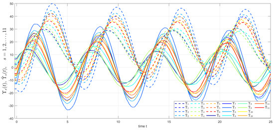
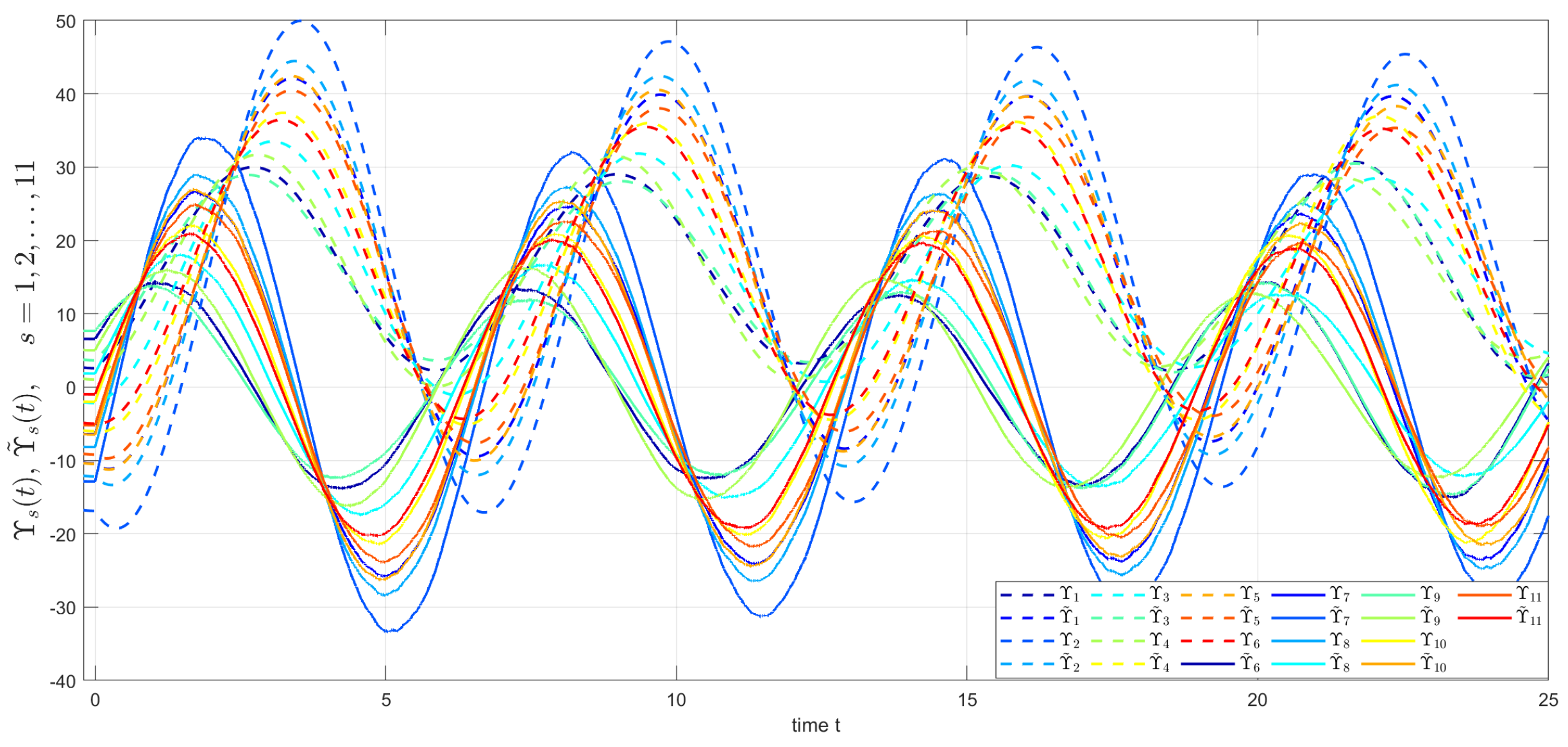
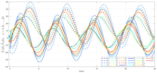
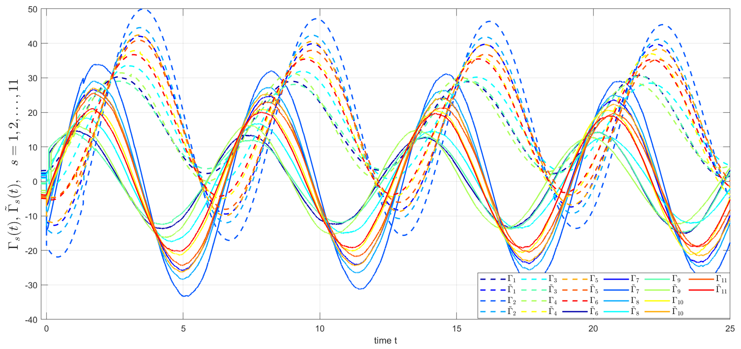
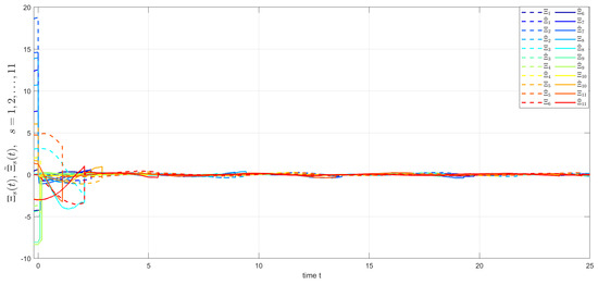
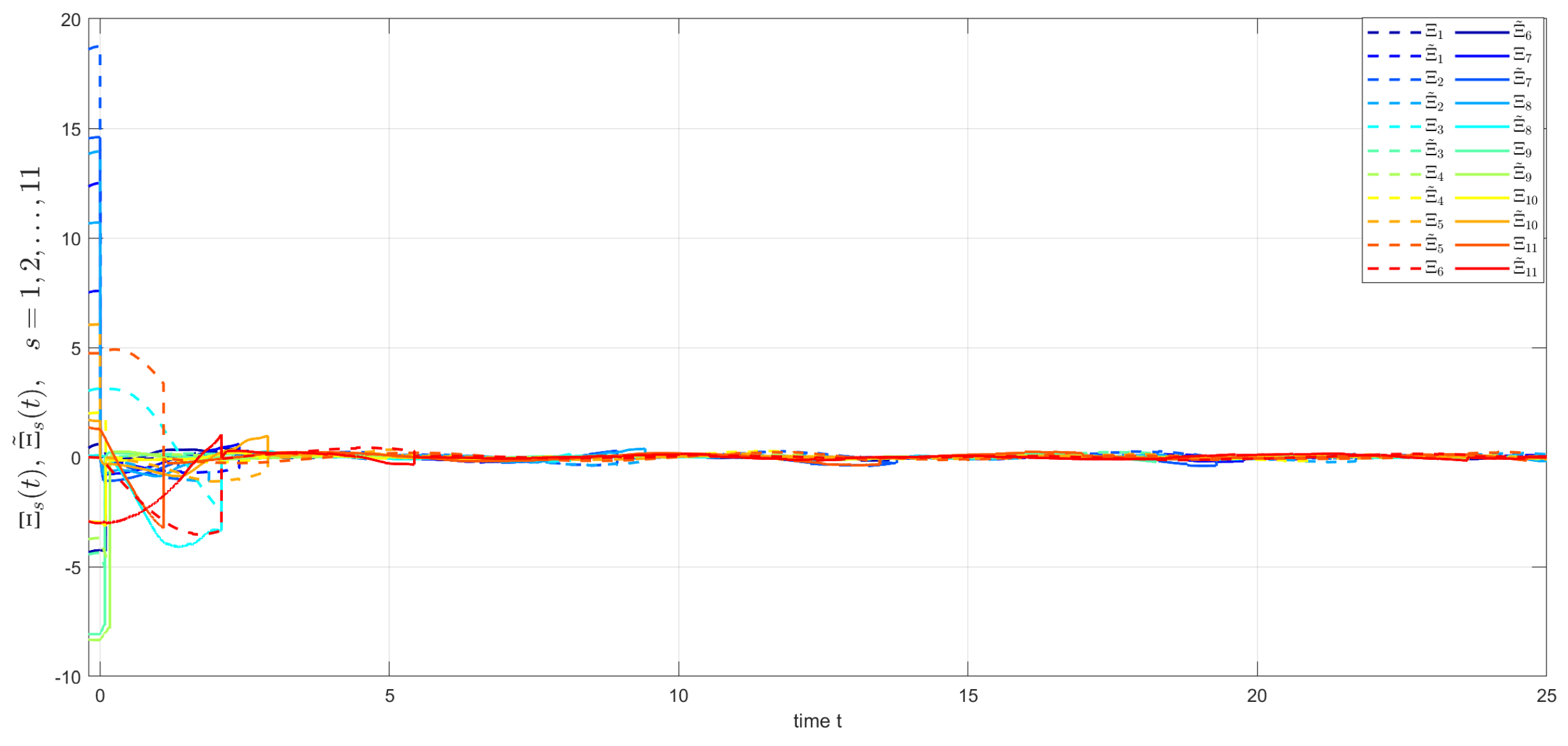
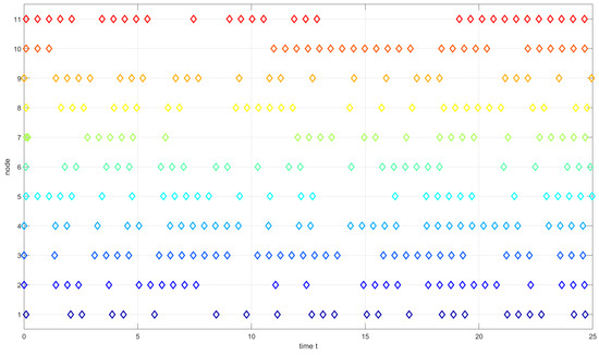
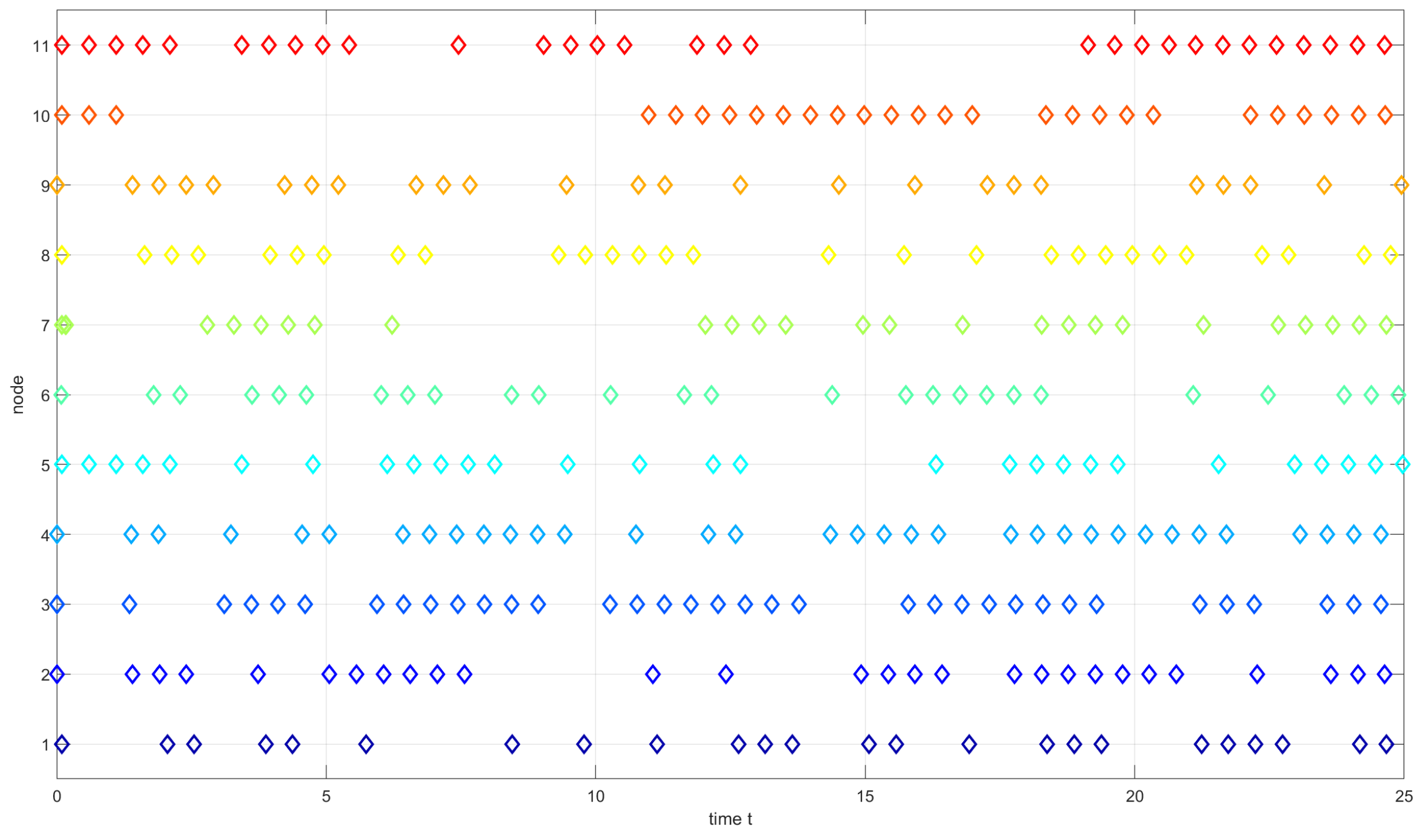
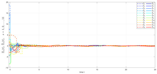
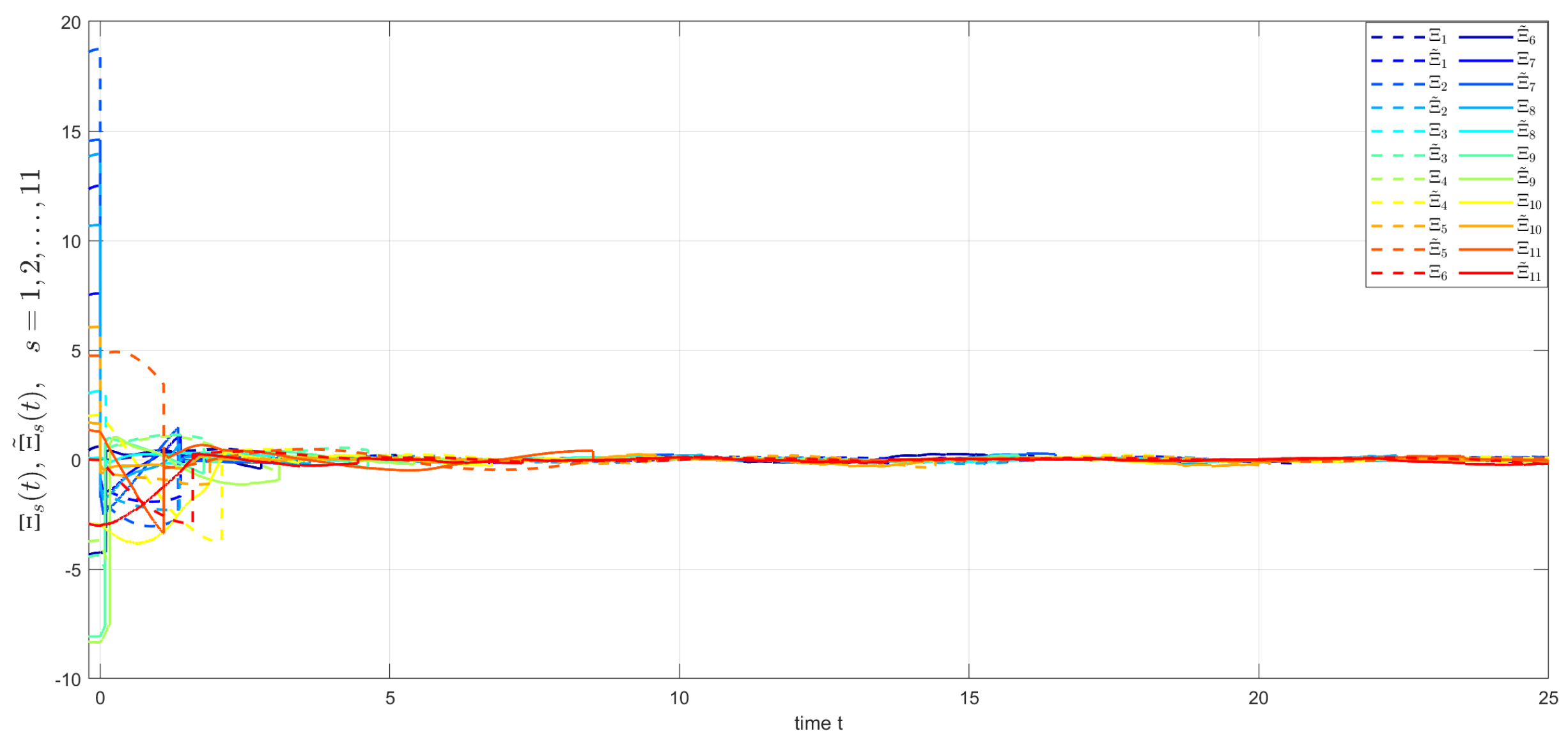
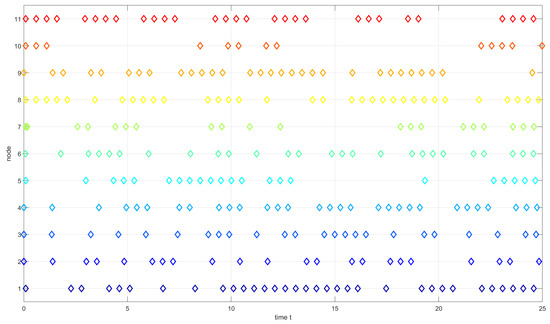
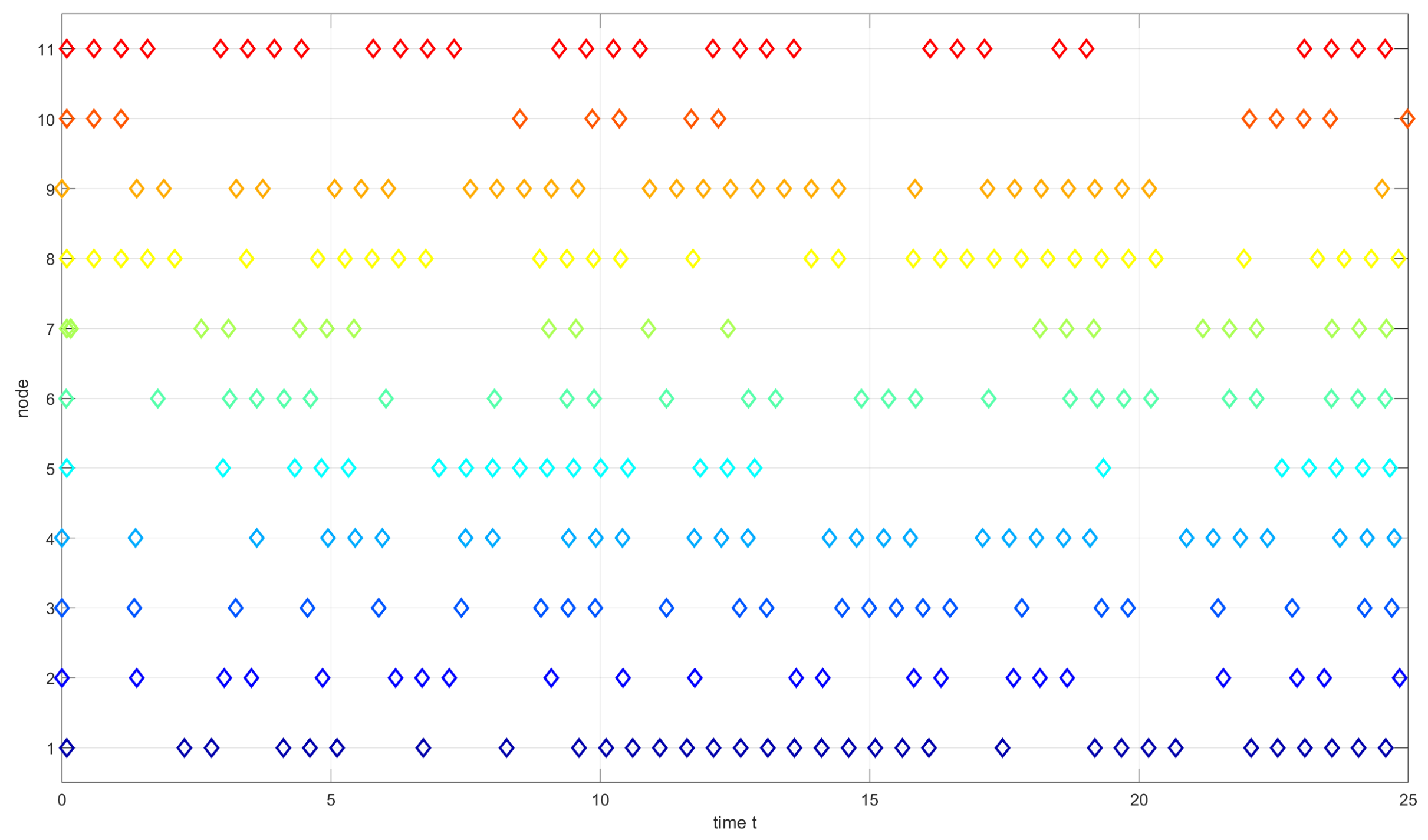
The following are the visualized simulation results. The motion trajectory of the systems (36) is plotted in Figure 1, while Figure 2 depicts that of the response system (37). As illustrated in Figure 3, the synchronization error is ultimately bounded through static self-triggered impulsive control. Figure 4 illustrates the number of triggering events under static self-triggered impulsive control. It follows that the number of triggering events for all nodes is about 312. Figure 5 plots the convergence of the bounded synchronization error of each node with the dynamic control. Meanwhile, the triggering moments under this control are displayed in Figure 6, with a total of almost 288 events. It can be noted that the addition of floating function has reduced the number of triggers. Therefore, the dynamic self-triggered impulsive control mechanism reduces resource consumption and better meets practical requirements.

Figure 1. The trajectories of all the nodes of the drive system.

Figure 2. The trajectories of all the nodes of the response system.

Figure 3. The trajectories of the bounded synchronization error of each node under static self-triggered impulsive control.

Figure 4. The triggering moments with the static self-triggered control mechanism.

Figure 5. Trajectories of the bounded synchronization error of each node under dynamic self-triggered impulsive control.

Figure 6. The triggering moments with the dynamic self-triggered control mechanism.

Table 1 illustrates that the goal of bounded synchronization is preserved under different settings of network sizes, attack probabilities, delay bounds, and noise intensity. The dynamic self-triggering scheme consistently results in a reduced number of control updates, thereby demonstrating enhanced resource economy relative to the static triggering mechanism.

Table 1. Synchronization under different parameter variations.

Case	Changed Parameter	Static Impulsive	Dynamic Impulsive	Synchronization
1	m = 21	576	542	Yes
2	$\varpi =0.5$, $\kappa =0.4$	268	251	Yes
3	$\tau =0.15$	261	240	Yes
4	noise intensity 0.02	330	312	Yes

6. Conclusions

Mean-square bounded synchronization was studied in stochastic CNs under cyber-attack via self-triggered impulsive control mechanisms. We proposed a self-triggered impulsive control approach that predicts the next impulse instant from the current system state. This approach incorporates both static and dynamic mechanisms, ensuring that the synchronization error converges to the desired state. In addition, we proposed a dual-Bernoulli scheme in which independent random variables are assigned to DoS and deception attacks, respectively, enabling their collaborative integration into the system model. Sufficient conditions for ensuring mean-square bounded synchronization were derived by the Lyapunov functional method. Meanwhile, Zeno behavior was effectively ruled out. Finally, through detailed simulation experiments, we illustrated the accuracy and applicability of the theoretical analysis. As illustrated by the comparative studies, the dynamic self-triggering mechanism effectively eliminates redundant triggers, which has the advantage of energy conservation. Future research will consider correlated cyber-attacks, burst attacks, and Markovian attack models to further improve the applicability of the proposed framework.

References

- Wu, Y.; Shen, B.; Ahn, C.K.; Li, W. Intermittent dynamic event-triggered control for synchronization of stochastic complex networks. IEEE Trans. Circuits Syst. I Regul. Pap. 2021, 68, 2639–2650. [Google Scholar] [CrossRef] [Scilit]
- Zhang, W.; Yang, X.; Yang, S.; Alsaedi, A. Finite-time and fixed-time bipartite synchronization of complex networks with signed graphs. Math. Comput. Simul. 2021, 188, 319–329. [Google Scholar] [CrossRef] [Scilit]
- Guo, Y.; Li, Y. Bipartite leader-following synchronization of fractional-order delayed multilayer signed networks by adaptive and impulsive controllers. Appl. Math. Comput. 2022, 430, 127243. [Google Scholar] [CrossRef] [Scilit]
- Wang, J.; Xu, C.; Feng, J.; Kwong, M.K.; Austin, F. Mean-square exponential synchronization of markovian switching stochastic complex networks with time-varying delays by pinning control. Abstr. Appl. Anal. 2012, 2012, 298095. [Google Scholar] [CrossRef] [Scilit]
- Selvaraj, P.; Sakthivel, R.; Kwon, O.M. Finite-time synchronization of stochastic coupled neural networks subject to Markovian switching and input saturation. Neural Netw. 2018, 105, 154–165. [Google Scholar] [CrossRef] [Scilit] [PubMed]
- Mu, G.; Li, L.; Li, X. Quasi-bipartite synchronization of signed delayed neural networks under impulsive effects. Neural Netw. 2020, 129, 31–42. [Google Scholar] [CrossRef] [Scilit] [PubMed]
- Hu, T.; Park, J.H.; Liu, X.; He, Z.; Zhong, S. Sampled-data-based event-triggered synchronization strategy for fractional and impulsive complex networks with switching topologies and time-varying delay. IEEE Trans. Syst. Man Cybern. Syst. 2022, 52, 3568–3580. [Google Scholar] [CrossRef] [Scilit]
- Wu, H.Y.; Wang, L.; Zhao, L.H.; Wang, J.L. Topology identification of coupled neural networks with multiple weights. Neurocomputing 2021, 257, 254–264. [Google Scholar] [CrossRef] [Scilit]
- Liu, Y.; Li, W.; Feng, J. The stability of stochastic coupled systems with time-varying coupling and general topology structure. IEEE Trans. Neural Netw. Learn. Syst. 2018, 29, 4189–4200. [Google Scholar] [CrossRef] [Scilit] [PubMed]
- Rakkiyappan, R.; Cao, J.; Velmurugan, G. Existence and uniform stability analysis of fractional-order complex-valued neural networks with time delays. IEEE Trans. Neural Netw. Learn. Syst. 2015, 26, 84–97. [Google Scholar] [CrossRef] [Scilit] [PubMed]
- Zou, L.; Wang, Z.; Gao, H.; Liu, X. Event-triggered state estimation for complex networks with mixed time delays via sampled data information: The continuous-time case. IEEE Trans. Cybern. 2015, 45, 2804–2815. [Google Scholar] [CrossRef] [Scilit] [PubMed]
- Yang, T.; Chen, G.; Xia, J.; Wang, Z.; Sun, Q. Robust H∞ filtering for polytopic uncertain stochastic systems under quantized sampled outputs. Appl. Math. Comput. 2019, 347, 688–701. [Google Scholar] [CrossRef] [Scilit]
- Zhuang, G.; Xia, J.; Feng, J.; Wang, Y.; Chen, G. Dynamic compensator design and H∞ admissibilization for delayed singular jump systems via Moore-Penrose generalized inversion technique. Nonlinear Anal. Hybrid Syst. 2023, 49, 101361. [Google Scholar] [CrossRef] [Scilit]
- Li, C.; Wu, H.Y.; Yang, C.; Liu, Q.; Cao, J.; Yu, T. Finite-time consensus for nonlinear uncertain PDE multi-agent systems with time-varying delays via boundary control. Inf. Sci. 2026, 754, 123736. [Google Scholar] [CrossRef] [Scilit]
- Chen, G.; Xia, J.; Zhuang, G.; Zhao, J. Improved delay-dependent stabilization for a class of networked control systems with nonlinear perturbations and two delay components. Appl. Math. Comput. 2018, 316, 1–17. [Google Scholar] [CrossRef] [Scilit]
- Zhuang, G.; Xia, J.; Feng, J.; Zhang, B.; Lu, J.; Wang, Z. Admissibility analysis and stabilization for neutral descriptor hybrid systems with time-varying delays. Nonlinear Anal. Hybrid Syst. 2019, 33, 311–321. [Google Scholar] [CrossRef] [Scilit]
- Wang, Y.; Zheng, W.X.; Zhang, H. Dynamic event-based control of nonlinear stochastic systems. IEEE Trans. Autom. Control 2017, 62, 6544–6551. [Google Scholar] [CrossRef] [Scilit]
- Liu, X.; Zhang, K. Stabilization of nonlinear time-delay systems: Distributed-delay dependent impulsive control. Systems 2018, 120, 17–22. [Google Scholar] [CrossRef] [Scilit]
- Huang, H.; Ho, D.W.C.; Lam, J. Stochastic stability analysis of fuzzy hopfield neural networks with time-varying delays. IEEE Trans. Circuits Syst. II Express Briefs 2005, 52, 251–255. [Google Scholar] [CrossRef] [Scilit]
- He, W.; Qian, F.; Lam, J.; Chen, G.; Han, Q.L.; Kurths, J. Quasi-synchronization of heterogeneous dynamic networks via distributed impulsive control: Error estimation, optimization and design. Automatica 2015, 61, 249–262. [Google Scholar] [CrossRef] [Scilit]
- Xu, D.; Zhang, Y.; Li, W. Quasi-synchronization of heterogeneous hybrid stochastic delayed networks via pinning intermittent discrete observation control. IEEE Trans. Autom. Sci. Eng. 2024, 22, 2051–2061. [Google Scholar] [CrossRef] [Scilit]
- Liu, X.; Tay, W.P.; Liu, Z.W.; Xiao, G. Quasi-synchronization of heterogeneous networks with a generalized markovian topology and event-triggered communication. IEEE Trans. Cybern. 2020, 50, 4200–4213. [Google Scholar] [CrossRef] [Scilit] [PubMed]
- Zhu, S.; Zhou, J.; Yu, X.; Lu, J. Bounded synchronization of heterogeneous complex dynamical networks: A unified approach. IEEE Trans. Autom. Control 2021, 66, 1756–1762. [Google Scholar] [CrossRef] [Scilit]
- Zhao, J.; Hill, D.J.; Liu, T. Global bounded synchronization of general dynamical networks with nonidentical nodes. IEEE Trans. Autom. Control 2012, 57, 2656–2662. [Google Scholar] [CrossRef] [Scilit]
- Chen, T.; Wang, W.; Wu, Y. Quasi-synchronization of fuzzy heterogeneous complex networks via intermittent discrete-time state observations control. IEEE Trans. Fuzzy Syst. 2022, 30, 3085–3097. [Google Scholar] [CrossRef] [Scilit]
- Wang, Z.; Jin, X.; Pan, L.; Feng, Y.; Cao, J. Quasi-synchronization of delayed stochastic multiplex networks via impulsive pinning control. IEEE Trans. Syst. Man Cybern. Syst. 2022, 52, 5389–5397. [Google Scholar] [CrossRef] [Scilit]
- Yang, J.; Li, H.L.; Yang, J. Quasi-synchronization and complete synchronization of fractional-order fuzzy BAM neural networks via nonlinear control. Neural Process. Lett. 2022, 54, 3303–3319. [Google Scholar] [CrossRef] [Scilit]
- Wang, L.; Qian, W.; Wang, Q.G. Bounded synchronisation of a time-varying dynamical network with nonidentical nodes. Int. J. Syst. Sci. 2013, 46, 1234–1245. [Google Scholar] [CrossRef] [Scilit]
- Zhong, W.S.; Liu, G.P.; Thomas, C. Global bounded consensus of multiagent systems with nonidentical nodes and time delays. IEEE Trans. Syst. Man. Cybern. Part B (Cybern.) 2012, 42, 1480–1488. [Google Scholar] [CrossRef] [Scilit] [PubMed]
- Zhang, X.; Pu, X.; Xu, L.; Wu, Y. Mean-square bounded consensus of nonlinear multi-agent systems with time-varying delays via impulsive control under dual-channel stochastic switching deception attacks. Int. J. Dyn. Control 2026, 14, 108. [Google Scholar] [CrossRef] [Scilit]
- Mo, W.; Bao, H. Mean-square bounded synchronization of fractional-order chaotic Lur’e systems under deception attack. Phys. A Stat. Mech. Its Appl. 2024, 641, 129726. [Google Scholar] [CrossRef] [Scilit]
- Yan, X.; Li, K.; Yang, C.; Zhuang, J.; Cao, J. Consensus of fractional-order multi-agent systems via observer-based boundary control. IEEE Trans. Netw. Sci. Eng. 2024, 11, 3370–3382. [Google Scholar] [CrossRef] [Scilit]
- Fu, S.; Li, L.; Feng, J. Strategy optimization of controlled evolutionary games on a two-layer coupled network using Lebesgue sampling. Nonlinear Anal. Hybrid Syst. 2025, 56, 101570. [Google Scholar] [CrossRef] [Scilit]
- Zhuang, J.; Peng, S.; Wang, Y. Event-triggered intermittent-based impulsive control for stabilization of nonlinear systems. IEEE Trans. Circuits Syst. II Express Briefs 2022, 69, 5039–5043. [Google Scholar] [CrossRef] [Scilit]
- Yu, N.; Zhu, W. Exponential stabilization of fractional-order continuous-time dynamic systems via event-triggered impulsive control. Nonlinear Anal. Model. Control 2022, 27, 592–608. [Google Scholar] [CrossRef] [Scilit]
- Li, X.; Peng, D.; Cao, J. Lyapunov stability for Impulsive Systems via Event-triggered Impulsive Control. IEEE Trans. Autom. Control 2020, 65, 4908–4913. [Google Scholar] [CrossRef] [Scilit]
- Ding, D.; Tang, Z.; Wang, Y.; Ji, Z.; Park, J.H. Secure synchronization for cyber-physical complex networks based on self-triggering impulsive control: Static and dynamic method. IEEE Trans. Netw. Sci. Eng. 2021, 8, 3167–3178. [Google Scholar] [CrossRef] [Scilit]
- Zhou, H.; Kong, D.; Park, J.H.; Li, W. Periodic self-triggered impulsive synchronization of hybrid stochastic complex-valued delayed networks. IEEE Trans. Control Netw. Syst. 2024, 11, 42–52. [Google Scholar] [CrossRef] [Scilit]
- Wang, M.; He, X.; Li, X. Self-triggered impulsive control for Lyapunov stability of nonlinear systems in discrete time. IEEE Trans. Cybern. 2024, 54, 4852–4858. [Google Scholar] [CrossRef] [Scilit] [PubMed]
- Xie, X.; Li, X.; Song, S.; Liu, X. A self-triggered impulsive approach to group consensus of MASs with sensing/actuation delays. IEEE Trans. Syst. Man Cybern. Syst. 2023, 54, 1168–1179. [Google Scholar] [CrossRef] [Scilit]
- Liu, D.; Ye, D. Pinning-observer-based secure synchronization control for complex dynamical networks subject to DoS attacks. IEEE Trans. Circuits Syst. I Regul. Pap. 2020, 67, 5394–5404. [Google Scholar] [CrossRef] [Scilit]
- Fu, W.; Qin, J.; Shi, Y.; Zheng, W.X.; Kang, Y. Resilient consensus of discrete-time complex cyber-physical networks under deception attacks. IEEE Trans. Ind. Inform. 2020, 16, 4868–4877. [Google Scholar] [CrossRef] [Scilit]
- Xu, X.; Li, X.; Dong, P.; Liu, Y. Robust reset speed synchronization control for an integrated motor-transmission powertrain system of a connected vehicle under a replay attack. IEEE Trans. Veh. Technol. 2021, 70, 5524–5536. [Google Scholar] [CrossRef] [Scilit]
- Zhang, Z.; Xue, L.; Wu, Y.; Liu, J.; Sun, C. Aperiodically intermittent event-triggered control for practical fixed-time consensus under denial-of-service attack. Nonlinear Dyn. 2024, 112, 21117–21134. [Google Scholar] [CrossRef] [Scilit]
- Wu, H.Y.; Liu, Q.; Park, J.H. Observer-based secure consensus for multiagent systems under multimode DoS attacks with application to power system. IEEE Trans. Cybern. 2025, 55, 1032–1044. [Google Scholar] [CrossRef] [Scilit] [PubMed]
- Lin, P.; Deng, F.; Zhao, X.; Wan, F.; Huang, Y. Stability analysis of networked stochastic systems with time delays under deception attacks by sampled-data control. IEEE Trans. Syst. Man Cybern. Syst. 2025, 55, 2950–2960. [Google Scholar] [CrossRef] [Scilit]
- Feng, J.; Xie, J.; Wang, J.; Zhao, Y. Secure synchronization of stochastic complex networks subject to deception attack with nonidentical nodes and internal disturbance. Inf. Sci. 2021, 547, 514–525. [Google Scholar] [CrossRef] [Scilit]
- Wang, Y.; Li, Y.; Parisini, T.; Zhao, D. Attacks with distributed adaptive strategies resilient distributed control for uncertain nonlinear interconnected systems under replay cyber-attacks. IEEE Trans. Autom. Control 2025, 70, 5429–5443. [Google Scholar] [CrossRef] [Scilit]
- Cheng, P.; He, S.; Xiao, G.; Zhang, W. HMM-based secure control of multiagent systems under DoS attacks. IEEE Trans. Autom. Control 2026, 71, 1199–1206. [Google Scholar] [CrossRef] [Scilit]
- Cheng, P.; He, S.; Xiao, G.; Zhang, W. ESO-based control for 2-D networked control systems with Markov-Type DoS attacks. IEEE Trans. Netw. Sci. Eng. 2025, 12, 4452–4461. [Google Scholar] [CrossRef] [Scilit]
- Cheng, P.; Wu, D.; Nie, R.; He, S.; Xiao, G. Sliding mode control for multiagent systems under DoS attacks: A reduced-order approach. IEEE Trans. Cybern. 2026, 56, 3515–3525. [Google Scholar] [CrossRef] [Scilit] [PubMed]
- Liang, X.; Xia, J.; Chen, G.; Zhang, H.; Wang, Z. Dissipativity-based sampled-data control for fuzzy Markovian jump systems. Appl. Math. Comput. 2019, 361, 552–564. [Google Scholar] [CrossRef] [Scilit]
- Zhao, Y.; Sun, L.; Chen, L.; Wang, Z. Aperiodic intermittent dynamic event-triggered synchronization control for stochastic delayed multi-links complex networks. Neural Netw. 2024, 180, 106658. [Google Scholar] [CrossRef] [Scilit] [PubMed]
- Yang, N.; Chen, S.; Su, H. Adaptive event-triggered impulsive control for stochastic complex networks with delays under deception attacks. Nonlinear Dyn. 2025, 113, 2259–2276. [Google Scholar] [CrossRef] [Scilit]
- Li, M.Y.; Shuai, Z. Global-stability problem for coupled systems of differential equations on networks. J. Differ. Equ. 2010, 248, 1–20. [Google Scholar] [CrossRef] [Scilit]
Disclaimer/Publisher’s Note: The statements, opinions and data contained in all publications are solely those of the individual author(s) and contributor(s) and not of MDPI and/or the editor(s). MDPI and/or the editor(s) disclaim responsibility for any injury to people or property resulting from any ideas, methods, instructions or products referred to in the content. |
© 2026 by the authors. Licensee MDPI, Basel, Switzerland. This article is an open access article distributed under the terms and conditions of the Creative Commons Attribution (CC BY) license.