Inequalities for ζ(s) − ψ(1 − s) Related to a Conjecture of Henry

Abstract

In this paper, we investigate analytic inequalities related to a conjecture of Henry involving the difference between the Riemann zeta function and the digamma function. By treating $\zeta \left(s\right)-\psi (1-s)$ as a unified analytic object, we establish its strict convexity and monotonicity on suitable intervals. Moreover, we obtain explicit boundary limits of the derivative, expressed in terms of $\pi$, $log\left(2\pi \right)$ and Stieltjes constants. These results lead to new inequalities for $\zeta \left(s\right)-\psi (1-s)$ and shed further light on the conjecture.

1. Introduction

The Riemann zeta function and the digamma function are among the most classical special functions in analytic number theory. Both play fundamental roles in the study of Dirichlet series, the Gamma function, and related analytic identities. Combinations of these functions often exhibit subtle cancellations, leading to refined analytic inequalities and unexpected structural properties. For more results on inequalities for the Riemann zeta function, we refer the reader to [1,2,3].

Motivated by these thoughts, we focus on the function

$$F\left(s\right)=\zeta \left(s\right)-\psi (1-s),$$

defined on the interval on $0<s<1$ (see Section 2 for precise definition). This difference naturally combines the analytic continuation of the Riemann zeta function with the logarithmic derivative of the Gamma function, and its behavior on the critical interval is far from obvious.

In [4], Henry proposed a conjecture concerning sharp linear bounds for the function $\zeta \left(s\right)-\psi \left(s\right)$, suggesting that it admits optimal inequalities closely related to classical constants such as $\pi$ and the Euler–Mascheroni constant ${\gamma }_0\approx 0.577216$.

Conjecture 1.

Define $b^{\prime }:={\gamma }_0+{\displaystyle \frac{1}{2}}$ and $b:={\gamma }_0-{\displaystyle \frac{1}{2}}$. Then, if $0<s<1$, we conjecture that the relation

$$\pi cot\left(\pi s\right)+s<\zeta \left(s\right)-\psi \left(s\right)<\pi cot\left(\pi s\right)+b^{\prime }s+b$$

(1)

holds.

Since

$$\psi (1-s)-\psi \left(s\right)=\pi cot\left(\pi s\right),$$

the inequality (1) is equivalent to

$$s<F\left(s\right)<b^{\prime }s+b.$$

Motivated by this conjecture, we investigate strict convexity and monotonicity of $F\left(s\right)$ on $(0, 1)$ and determine the precise boundary behavior $F^{\prime }\left(s\right)$, obtaining explicit constants involving $\pi$, $log\left(2\pi \right)$, and the first Stieltjes constant. Our approach relies on Stieltjes expansions of the Riemann zeta function with series representations of the digamma function and sharp asymptotic estimates, which may be applicable to other combinations of special functions. Our main theorem is as follows.

Theorem 1.

Let $F\left(s\right)=\zeta \left(s\right)-\psi (1-s)$ be a real-valued function defined on the interval $0<s<1$. Then, the following assertions hold:

• $F^{″}\left(s\right)>0$ for all $s\in (0, 1)$; i.e., F is strictly convex on $(0, 1)$.
• $F^{\prime }\left(s\right)>0$ for all $s\in (0, 1)$; i.e., F is strictly increasing on $(0, 1)$.
• The boundary behavior of $F^{\prime }\left(s\right)$ is given by

  $$\underset{s\to 0^{+}}{lim}{F}^{\prime }\left(s\right)={\displaystyle \frac{{\pi }^2}{6}}-{\displaystyle \frac{1}{2}}log\left(2\pi \right),\underset{s\to 1^{-}}{lim}{F}^{\prime }\left(s\right)={\displaystyle \frac{{\pi }^2}{6}}-{\gamma }_1.$$

The following corollary, which follows from Theorem 1, implies Conjecture 1.

Corollary 1.

For $0<s<1$, we have the following inequality,

$$s<F\left(s\right)<b^{\prime }s+b,$$

where $b^{\prime }s+b$ is the best possible linear upper bound for $F\left(s\right)$ on $(0, 1)$.

Remark 1.

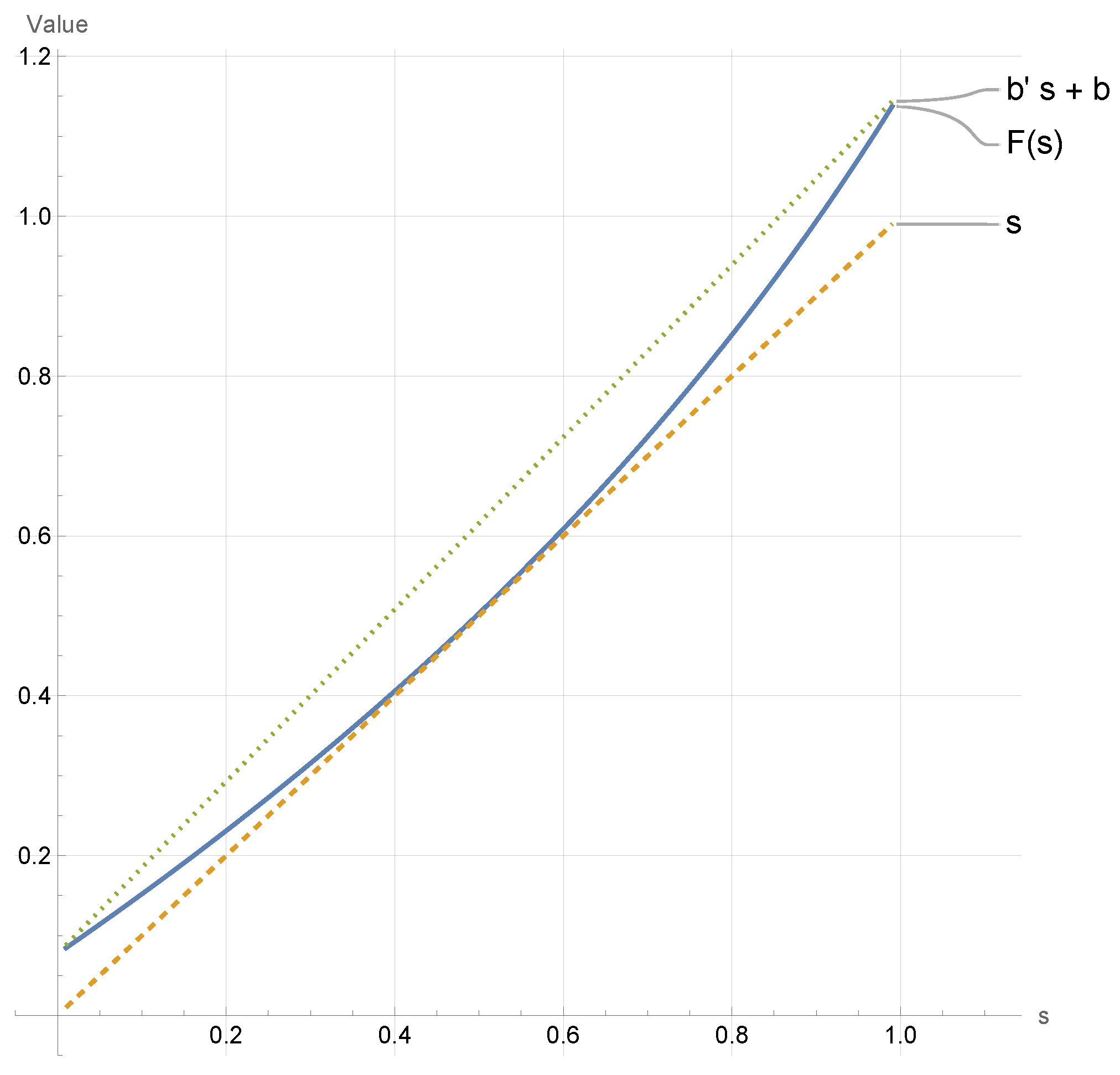
Figure 1 illustrates the behavior of the functions involved in the conjectured inequality

$$s<F\left(s\right)<b^{\prime }s+b(0<s<1).$$

The plot serves to provide intuition for the validity of the conjecture and to visualize the bounds, while the proof relies entirely on analytic arguments.

Remark 2.

It has been observed in the literature that inequalities of the type considered in this conjecture are related to certain elementary criteria for the Riemann hypothesis. In particular, assuming the conjecture holds, one may reformulate aspects of the Riemann hypothesis in terms of the behavior of $\zeta \left(x\right)$ on the interval $0<x<1$. We do not pursue this direction here and refer the reader to [5,6] for a detailed analysis.

2. Preliminaries

In this section, we collect several analytic facts concerning the Riemann zeta function and the digamma function that will be used throughout the proof of our main results.

We recall that the Riemann zeta function is defined for $\mathrm{Re}\left(s\right)>1$ by the absolutely convergent Dirichlet series

$$\zeta \left(s\right)={\displaystyle \sum _{n=1}^{\infty }}{\displaystyle \frac{1}{n^s}},$$

and admits a meromorphic continuation to the whole complex plane with a simple pole at $s=1$. In particular, its Laurent expansion at $s=1$ is given by

$$\zeta \left(s\right)={\displaystyle \frac{1}{s-1}}+{\displaystyle \sum _{k=0}^{\infty }}{\displaystyle \frac{{(-1)}^k{\gamma }_k{(s-1)}^k}{k!}},$$

(2)

where ${\gamma }_k$ denote the Stieltjes constants (see Stieltjes’s paper [7] and Ferguson’s work [8]). For $k=0$, this reduces to the Euler–Mascheroni constant ${\gamma }_0$.

We also recall that the digamma function is defined by

$$\psi \left(s\right)={\displaystyle \frac{{\Gamma }^{\prime }\left(s\right)}{\Gamma \left(s\right)}},$$

where $\Gamma$ denotes the usual gamma function. The digamma function $\psi \left(s\right)$ is related to the Riemann zeta function. For example, one has the expansion

$$\psi (s+1)=-{\gamma }_0+{\displaystyle \sum _{j=2}^{\infty }}{(-1)}^j\zeta \left(j\right)s^{j-1},\left|s\right|<1.$$

(3)

Moreover, for $\mathrm{Re}\left(s\right)>0$, the digamma function admits the integral representation:

$$\psi \left(s\right)+{\gamma }_0={\int }_0^1{\displaystyle \frac{1-x^{s-1}}{1-x}}dx.$$

(4)

As shown in [9] (p. 25), the representation (4) can be derived from the expansion (3).

Before proving the main theorem, we also establish several auxiliary lemmas that will be used in the sequel.

Lemma 1

([9]). When $\mathrm{Re}\left(s\right)>-1$ holds, the relation

$$\zeta \left(s\right)+{\displaystyle \frac{1}{1-s}}={\displaystyle \frac{1}{2}}-s{\int }_1^{\infty }{\displaystyle \frac{\left\{t\right\}-\frac{1}{2}}{t^{s+1}}}dt$$

holds, where $\left\{t\right\}$ denotes the fractional part of t.

Lemma 2.

Let $f\in C^2\left([0, 1]\right)$. Then

$${\int }_0^1\left(u-{\displaystyle \frac{1}{2}}\right)f\left(u\right)du={\displaystyle \frac{\left(f\right(1)-f(0\left)\right)}{8}}-{\displaystyle \frac{(f^{\prime }\left(1\right)+f^{\prime }\left(0\right))}{48}}+{\int }_0^1{\displaystyle \frac{{\left(u-\frac{1}{2}\right)}^3}{6}}{f}^{″}\left(u\right)du.$$

Proof. 

The result follows directly from integration by parts. □

Lemma 3.

The improper integrals

$${\int }_1^{\infty }{\displaystyle \frac{\left\{t\right\}-\frac{1}{2}}{t^{s+1}}}dt\mathit{and}{\int }_0^1{\displaystyle \frac{1-t^{-s}}{1-t}}dt$$

converge uniformly for s on any closed subinterval of $(0, 1)$. Moreover, for any positive integer m, the integrals obtained by differentiating m times with respect to s also converge uniformly on such subintervals.

Proof. 

Fix $0<a<b<1$. We prove uniform convergence on $[a, b]$. Let

$$I_1\left(s\right):={\int }_1^{\infty }{\displaystyle \frac{\left\{t\right\}-\frac{1}{2}}{t^{s+1}}}dt,I_2\left(s\right):={\int }_0^1{\displaystyle \frac{1-t^{-s}}{1-t}}dt.$$

Uniform convergence of $I_1$:

Since $|\left\{t\right\}-\frac{1}{2}|\le \frac{1}{2}$, for $t\ge 1$ and $s\in [a, b]$,

$$\left|{\displaystyle \frac{\left\{t\right\}-\frac{1}{2}}{t^{s+1}}}\right|\le {\displaystyle \frac{1}{2}}{t}^{-a-1},$$

and the majorant $t^{-a-1}$ is integrable on $[1,\infty )$. Hence, ${\int }_1^{\infty }(\left\{t\right\}-{\displaystyle \frac{1}{2}})t^{-s-1}dt$ converges uniformly for $s\in [a,b]$ by the Cauchy criterion for improper integrals.

Uniform convergence of $I_2$: We split the interval into $(0, {\displaystyle \frac{1}{2}}]$ and $[{\displaystyle \frac{1}{2}}, 1)$.

(i)

For $0<t\le {\displaystyle \frac{1}{2}}$, since $1/(1-t)\le 2$, we get

$$\left|{\displaystyle \frac{1-t^{-s}}{1-t}}\right|\le 2(1+t^{-s})\le 2(1+t^{-b}).$$

Since $b<1$, the function $1+t^{-b}$ is integrable on $(0, {\displaystyle \frac{1}{2}}]$.

(ii)

For ${\displaystyle \frac{1}{2}}\le t<1$, we use the mean value theorem. Applied to the function $x\mapsto x^{-s}$ on $[t, 1]$, it gives some $\xi \in (t, 1)$ such that

$$1-t^{-s}=-s{\xi }^{-s-1}(1-t).$$

Therefore

$$\left|{\displaystyle \frac{1-t^{-s}}{1-t}}\right|=s{\xi }^{-s-1}\le b{2}^{b+1},$$

because $s\le b$ and $\xi \ge {\displaystyle \frac{1}{2}}$. Hence, the integrand is uniformly bounded on $[{\displaystyle \frac{1}{2}}, 1]$.

Combining the two estimates, the uniform convergence of $I_2\left(s\right)$ on $[a, b]$ follows.

Derivatives with respect to s: For $m=1, 2$, differentiating under the integral sign yields integrands of the form

$${(logt)}^m{\displaystyle \frac{\left\{t\right\}-\frac{1}{2}}{t^{s+1}}}\mathrm{and}{\displaystyle \frac{{(logt)}^m{t}^{-s}}{1-t}}.$$

Arguing as above, these are dominated on $[a, b]$ by integrable functions $t^{-a-1}{(logt)}^m$ on $[1,\infty )$ and ${(log(1/t))}^m{t}^{-b}$ on $(0, 1)$, respectively. Hence, by a similar argument, the corresponding improper integrals converge uniformly on $[a, b]$. □

We recall the following lemma from ([10], p. 67).

Lemma 4.

Let

$$F\left(s\right)=D\left(f\right)\left(s\right):={\displaystyle \sum _{n=1}^{\infty }}{\displaystyle \frac{f\left(n\right)}{n^s}}$$

be a Dirichlet series convergent in the half-plane $\mathrm{Re}\left(s\right)>\sigma$. Then, for every integer $k\ge 1$, the series $F\left(s\right)$ is k times termwise differentiable in the half-plane $\mathrm{Re}\left(s\right)>\sigma$, i.e.,

$$F^{\left(k\right)}\left(s\right)={(-1)}^k{\displaystyle \sum _{n=1}^{\infty }}{\displaystyle \frac{f\left(n\right){(logn)}^k}{n^s}},\mathrm{Re}\left(s\right)>\sigma .$$

The Riemann zeta function converges on $\mathrm{Re}\left(s\right)>1$. By Lemma 4, we obtain the following proposition.

Proposition 1.

If s is the complex number satisfying $\mathrm{Re}\left(s\right)>1$, then

$${\displaystyle \sum _{n=1}^{\infty }}{\displaystyle \frac{log\left(n\right)}{n^s}}=-{\zeta }^{\prime }\left(s\right),{\displaystyle \sum _{n=1}^{\infty }}{\displaystyle \frac{{log}^2\left(n\right)}{n^s}}={\zeta }^{″}\left(s\right),{\displaystyle \sum _{n=1}^{\infty }}{\displaystyle \frac{{log}^3\left(n\right)}{n^s}}=-{\zeta }^{‴}\left(s\right).$$

Moreover, when $s\in \mathbb{R}$ and $2<s<3$,

$${\zeta }^{\prime }\left(s\right)<0,{\zeta }^{″}\left(s\right)>0,{\zeta }^{‴}\left(s\right)<0.$$

3. Proof of Our Main Result

We now turn to the proof of our main results.

Proof of Theorem 1.

We prove the assertions in the order $\left(1\right)\to \left(3\right)\to \left(2\right)$.

Proof of (1): Fix $s\in (0, 1)$. Choose ${ϵ}_s>0$ sufficiently small such that ${ϵ}_s<s<1-{ϵ}_s$. By Equation (4) and Lemma 1,

$$F\left(s\right)={\displaystyle \frac{1}{2}}-s{\int }_1^{\infty }{\displaystyle \frac{\left\{t\right\}-\frac{1}{2}}{t^{s+1}}}dt+{\displaystyle \frac{1}{s-1}}-{\int }_0^1{\displaystyle \frac{1-t^{-s}}{1-t}}dt+{\gamma }_0.$$

Since the integrands, together with their partial derivatives with respect to s, are continuous and converge uniformly for s on the interval ${ϵ}_s\le s\le 1-{ϵ}_s$ by Lemma 3, the following computation is justified. Differentiate term by term and we obtain

$$F^{\prime }\left(s\right)={\int }_1^{\infty }{\displaystyle \frac{(\left\{t\right\}-\frac{1}{2})(slogt-1)}{t^{s+1}}}dt-{\displaystyle \frac{1}{{(s-1)}^2}}-{\int }_0^1{\displaystyle \frac{t^{-s}log\left(t\right)}{1-t}}dt.$$

Differentiate again and we obtain

$$F^{″}\left(s\right)={\int }_1^{\infty }{\displaystyle \frac{(\left\{t\right\}-\frac{1}{2})(2-slog\left(t\right))(log\left(t\right))}{t^{s+1}}}dt+{\displaystyle \frac{2}{{(s-1)}^3}}+{\int }_0^1{\displaystyle \frac{t^{-s}{log}^2\left(t\right)}{1-t}}dt.$$

Let

$$J\left(s\right):={\int }_1^{\infty }{\displaystyle \frac{(\left\{t\right\}-\frac{1}{2})(2-slogt)(logt)}{t^{s+1}}}dt$$

and

$$P\left(s\right):={\displaystyle \frac{2}{{(s-1)}^3}}+{\int }_0^1{\displaystyle \frac{t^{-s}{log}^{2}t}{1-t}}dt={\displaystyle \frac{2}{{(s-1)}^3}}-{\psi }^{″}(1-s).$$

To prove the convexity of $F\left(s\right)$, it suffices to show that $0<P\left(s\right)<\infty$ and $\left|J\right(s\left)\right|<P\left(s\right)$.

By the classical identity ${\psi }^{″}\left(s\right)=-2{\displaystyle \sum _{n=0}^{\infty }}{\displaystyle \frac{1}{{(n+s)}^3}}$, it follows that

$$P\left(s\right)={\displaystyle \sum _{n=2}^{\infty }}{\displaystyle \frac{2}{{(n-s)}^3}}.$$

Consequently, for $0<s<1$,

$$P\left(s\right)={\displaystyle \sum _{n=2}^{\infty }}{\displaystyle \frac{2}{{(n-s)}^3}}\ge 2{\displaystyle \sum _{n=2}^{\infty }}{\displaystyle \frac{1}{n^3}}=2(\zeta \left(3\right)-1)\approx 0.40411380632.$$

Meanwhile,

$$P\left(s\right)={\displaystyle \sum _{n=2}^{\infty }}{\displaystyle \frac{2}{{(n-s)}^3}}\le {\displaystyle \sum _{n=2}^{\infty }}{\displaystyle \frac{2}{{(n-1)}^3}}=2\zeta \left(3\right)<\infty .$$

To complement this estimate, we now consider the integral term $J\left(s\right)$. Let

$$g\left(x\right)={\displaystyle \frac{(2-slogx)logx}{x^{s+1}}}.$$

Then

$$\begin{array}{cc}\hfill J\left(s\right)& ={\int }_1^{\infty }\left(\left\{t\right\}-{\displaystyle \frac{1}{2}}\right)g\left(t\right)dt\hfill \\ & ={\displaystyle \sum _{n=1}^{\infty }}{\int }_n^{n+1}\left(\left\{t\right\}-{\displaystyle \frac{1}{2}}\right)g\left(t\right)dt\hfill \\ & ={\displaystyle \sum _{n=1}^{\infty }}{\int }_0^1\left(t-{\displaystyle \frac{1}{2}}\right)g(n+t)dt.\hfill \end{array}$$

It is easy to compute that

$$g^{\prime }\left(x\right)={\displaystyle \frac{2-(4s+2)logx+s(s+1){log}^{2}x}{x^{s+2}}},$$

and

$$g^{″}\left(x\right)={\displaystyle \frac{-6(s+1)+(6s^2+12s+4)logx-s(s+1)(s+2){log}^{2}x}{x^{s+3}}}.$$

Therefore, by Lemma 2,

$$\begin{array}{cc}\hfill J\left(s\right)& ={\displaystyle \frac{1}{8}}{\displaystyle \sum _{n=1}^{\infty }}(g(n+1)-g\left(n\right))-{\displaystyle \frac{1}{48}}{\displaystyle \sum _{n=1}^{\infty }}(g^{\prime }(n+1)+g^{\prime }\left(n\right))\hfill \\ \hfill & +{\displaystyle \frac{1}{6}}{\displaystyle \sum _{n=1}^{\infty }}{\int }_0^1{(t-{\displaystyle \frac{1}{2}})}^3{g}^{″}(n+t)dt\hfill \\ \hfill & :=I_1+I_2+I_3.\hfill \end{array}$$

We proceed to estimate the three terms separately.

Estimate of $I_1$: It is easy to follow that

$$I_1={\displaystyle \frac{1}{8}}{\displaystyle \sum _{n=1}^{\infty }}(g(n+1)-g\left(n\right))={\displaystyle \frac{1}{8}}\underset{N\to \infty }{lim}{\displaystyle \sum _{n=1}^N}(g(n+1)-g\left(n\right))=-{\displaystyle \frac{1}{8}}g\left(1\right)=0.$$

Estimate of $I_2$: By Proposition 1, we have

$${\displaystyle \sum _{n=1}^{\infty }}(g^{\prime }(n+1)+g^{\prime }\left(n\right))=4\zeta (s+2)-2+(8s+4){\zeta }^{\prime }(s+2)+s(s+1){\zeta }^{″}(s+2),$$

and the functions $\zeta$ and ${\zeta }^{″}$ are strictly decreasing on $(2, 3)$ and ${\zeta }^{\prime }$ is strictly increasing $(2, 3)$. In addition, we have $\zeta >0$ and ${\zeta }^{″}>0$, whereas ${\zeta }^{\prime }<0$ on this interval. Then

$$\begin{array}{cc}\hfill & 4\zeta (s+2)-2+(8s+4){\zeta }^{\prime }(s+2)+s(s+1){\zeta }^{″}(s+2)\hfill \\ \hfill & \le 4\zeta \left(2\right)-2+4{\zeta }^{\prime }\left(3\right)+2{\zeta }^{″}\left(2\right)\approx 7.765791.\hfill \end{array}$$

Hence

$$|I_2|\le {\displaystyle \frac{1}{48}}{\displaystyle \sum _{n=1}^{\infty }}(g^{\prime }(n+1)+g^{\prime }\left(n\right))\le {\displaystyle \frac{7.765791}{48}}=0.161787.$$

Estimate of $I_3$: Denote

$${\displaystyle \frac{1}{6}}{\int }_0^1{(t-{\displaystyle \frac{1}{2}})}^3{g}^{″}(n+t)dt$$

by $E_n\left(s\right)$. Then, $I_3={\displaystyle \sum _{n=1}^{\infty }}{E}_n$. We have

$$|E_n\left(s\right)|\le \underset{t\in [0,1]}{sup}|g^{″}(n+t)|{\int }_0^1\left|{\displaystyle \frac{{(u-\frac{1}{2})}^3}{6}}\right|du={\displaystyle \frac{1}{192}}\underset{t\in [0,1]}{sup}|g^{″}(n+t)|,$$

since ${\int }_0^1|{(u-{\displaystyle \frac{1}{2}})}^3|du={\displaystyle \frac{1}{32}}$.

One can notice that

$$\begin{array}{cc}\hfill & {\displaystyle \sum _{n=1}^{\infty }}\underset{t\in [0,1]}{sup}|g^{″}(n+t)|\hfill \\ \hfill & ={\displaystyle \sum _{n=1}^{\infty }}\underset{t\in [0,1]}{sup}\left|{\displaystyle \frac{-6(s+1)+(6s^2+12s+4)log(t+n)-s(s+1)(s+2){log}^2(t+n)}{{(t+n)}^{s+3}}}\right|\hfill \\ \hfill & \le {\displaystyle \sum _{n=1}^{\infty }}{\displaystyle \frac{6{log}^2(1+n)+22log(1+n)+12}{n^3}}.\hfill \end{array}$$

Hence

$${\displaystyle \sum _{n=1}^{\infty }}|E_n\left(s\right)|\le {\displaystyle \frac{1}{192}}{\displaystyle \sum _{n=1}^{\infty }}{\displaystyle \frac{6{log}^2(n+1)+22log(n+1)+12}{n^3}}=:{\displaystyle \frac{1}{192}}\Sigma .$$

To estimate $\Sigma$, fix $N\ge 2$ and split $\Sigma ={\Sigma }_{\le N}+{\Sigma }_{>N}$, where

$${\Sigma }_{\le N}:={\displaystyle \sum _{n=1}^N}{\displaystyle \frac{6{log}^2(n+1)+22log(n+1)+12}{n^3}}.$$

For the tail, note that for $x\ge 1$ we have $log(x+1)\le log\left(2x\right)=logx+log2$. Then,

$$\begin{array}{cc}\hfill {\Sigma }_{>N}& \le {\int }_N^{\infty }{\displaystyle \frac{6{log}^2(x+1)+22log(x+1)+12}{x^3}}dx\hfill \\ \hfill & \le {\int }_N^{\infty }{\displaystyle \frac{6{(logx+log2)}^2+22(logx+log2)+12}{x^3}}dx.\hfill \end{array}$$

The latter integral can be evaluated explicitly by integration by parts, giving a closed-form upper bound of the shape

$${\Sigma }_{>N}\le {\displaystyle \frac{3{(logN)}^2+(14+6log\left(2\right))logN+(13+14log\left(2\right)+3{log}^2\left(2\right))}{N^2}}.$$

Taking $N=200$, via Mathematica, a direct computation of ${\Sigma }_{\le 200}$ together with the above explicit tail estimate yields

$$\Sigma <40.697,$$

and therefore

$$I_3\le {\displaystyle \sum _{n=1}^{\infty }}\left|E_n\left(s\right)\right|\le {\displaystyle \frac{\Sigma }{192}}<{\displaystyle \frac{40.697}{192}}\approx 0.211964,$$

uniformly for all $0<s<1$.

All in all,

$$\begin{array}{cc}\hfill \left|J\right(s\left)\right|& \le |I_1|+|I_2|+|I_3|\hfill \\ \hfill & \le 0.161787+0.211964=0.373751<0.40411380632\le P\left(s\right).\hfill \end{array}$$

This completes the proof of (1).

Proof of (3): We study the behavior of $F^{\prime }\left(s\right)={\zeta }^{\prime }\left(s\right)+{\psi }^{\prime }(1-s)$ as $s\to 1^{-}$ and $s\to 0^{+}$.

Behavior as $s\to 1^{-}$: First, recall the Laurent expansion of the Riemann zeta function at $s=1$,

$$\zeta \left(s\right)={\displaystyle \frac{1}{s-1}}+{\displaystyle \sum _{k=0}^{\infty }}{\displaystyle \frac{{(-1)}^k{\gamma }_k{(s-1)}^k}{k!}},$$

which implies

$${\zeta }^{\prime }\left(s\right)=-{\displaystyle \frac{1}{{(s-1)}^2}}+{\displaystyle \sum _{k=1}^{\infty }}{\displaystyle \frac{{(-1)}^k{\gamma }_k{(s-1)}^{k-1}}{(k-1)!}}.$$

In particular, the finite part of ${\zeta }^{\prime }\left(s\right)$ at $s=1$ equals $-{\gamma }_1$.

Next, we use the classical power series expansion of the digamma function by [11],

$$\psi (z+1)=\psi \left(z\right)+{\displaystyle \frac{1}{z}}=-{\gamma }_0+{\displaystyle \sum _{j=2}^{\infty }}{(-1)}^j\zeta \left(j\right)z^{j-1},\left|z\right|<1.$$

(5)

Differentiating termwise, we obtain

$${\psi }^{\prime }\left(z\right)={\displaystyle \frac{1}{z^2}}+{\displaystyle \sum _{j=2}^{\infty }}{(-1)}^j\zeta \left(j\right)(j-1)z^{j-2}.$$

Replacing z by $1-s$ yields

$${\psi }^{\prime }(1-s)={\displaystyle \frac{1}{{(1-s)}^2}}+{\displaystyle \sum _{j=2}^{\infty }}{(-1)}^j\zeta \left(j\right)(j-1){(1-s)}^{j-2}.$$

Combining the above expansions,

$$\underset{s\to 1^{-}}{lim}{F}^{\prime }\left(s\right)=\underset{s\to 1^{-}}{lim}({\zeta }^{\prime }\left(s\right)+{\psi }^{\prime }(1-s))=-{\gamma }_1+\zeta \left(2\right)={\displaystyle \frac{{\pi }^2}{6}}-{\gamma }_1,$$

Behavior as $s\to 0^{+}$: It is well known that ${\zeta }^{\prime }\left(0\right)=-{\displaystyle \frac{1}{2}}log\left(2\pi \right)$. By taking $z=-s$ in Formula (5), we have

$$\psi (1-s)=-{\gamma }_0-{\displaystyle \sum _{j=2}^{\infty }}\zeta \left(j\right)s^{j-1},\left|s\right|<1.$$

Differentiating termwise, we obtain

$${\displaystyle \frac{d}{ds}}\psi (1-s)=-{\displaystyle \sum _{j=2}^{\infty }}\zeta \left(j\right)(j-1)s^{j-2},\left|s\right|<1.$$

Hence, $\underset{s\to 0^{+}}{lim}{\displaystyle \frac{d}{ds}}\psi (1-s)=-\zeta \left(2\right)$. All in all,

$$\underset{s\to 0^{+}}{lim}{F}^{\prime }\left(s\right)=-{\displaystyle \frac{1}{2}}log\left(2\pi \right)+\zeta \left(2\right)={\displaystyle \frac{{\pi }^2}{6}}-{\displaystyle \frac{1}{2}}log\left(2\pi \right),$$

which completes the proof of (3).

Proof of (2): It follows immediately from (1) and (3). □

Now we give the proof of Corollary 1.

Proof of Corollary 1.

Since

$$\pi cot\left(\pi s\right)=\psi (1-s)-\psi \left(s\right),$$

the inequality (1) is equivalent to

$$s<\zeta \left(s\right)-\psi (1-s)<b^{\prime }s+b.$$

A direct computation can obtain $F\left(0\right)=\zeta \left(0\right)-\psi \left(1\right)=-{\displaystyle \frac{1}{2}}+{\gamma }_0$. Using Formulas (2) and (3), it is easy to obtain that $\underset{s\to 1^{-}}{lim}F\left(s\right)=2{\gamma }_0$. Then, by Theorem 1 (1),

$$\zeta \left(s\right)-\psi (1-s)=F\left(s\right)<F\left(0\right)+(F\left(1\right)-F\left(0\right))s=({\gamma }_0-{\displaystyle \frac{1}{2}})+({\gamma }_0+{\displaystyle \frac{1}{2}})s.$$

This establishes the right side of the inequality.

Let $G\left(s\right)=F\left(s\right)-s$. Since

$$\underset{s\to 0^{+}}{lim}{G}^{\prime }\left(s\right)={\displaystyle \frac{{\pi }^2}{6}}-{\displaystyle \frac{1}{2}}log\left(2\pi \right)-1<0,\underset{s\to 1^{-}}{lim}{G}^{\prime }\left(s\right)={\displaystyle \frac{{\pi }^2}{6}}-{\gamma }_1-1>0.$$

$G\left(s\right)$ hasa unique minimum $s_0$ in $(0, 1)$ such that $G^{\prime }\left(s_0\right)=0$. Via Mathematica, $s_0\approx 0.484993$ and $G\left(s_0\right)\approx 0.00306469>0$. Hence, $G\left(s\right)>0$ for $s\in (0, 1)$ and the left side of the inequality is established. Moreover,

$$\underset{s\to 1^{-}}{lim}F\left(s\right)=\underset{s\to 1^{-}}{lim}(b^{\prime }s+b)=2{\gamma }_0.$$

So $b^{\prime }s+b$ is the best possible linear upper bound for $F\left(s\right)$ on $(0, 1)$, which completes the proof of Corollary 1. □

4. Concluding Remarks

Hurwitz [12] introduced the zeta function

$$\zeta (s,q)={\displaystyle \sum _{n=0}^{\infty }}{\displaystyle \frac{1}{{(n+q)}^s}},$$

which is now known as the Hurwitz zeta function. It is one generalization of the Riemann zeta function. Berndt gave the Laurent series of the Hurwitz zeta function in [13], i.e.,

$$\zeta (s,q)={\displaystyle \frac{1}{s-1}}+{\displaystyle \sum _{k=0}^{\infty }}{\displaystyle \frac{{(-1)}^k{\gamma }_k\left(q\right){(s-1)}^k}{k!}},$$

where ${\gamma }_k\left(q\right)$ denotes the k-th generalized Stieltjes constant.

Although the Hurwitz zeta function shares many analytic properties with the Riemann zeta function, the presence of the additional parameter q makes the derivation of explicit inequalities more delicate. It would therefore be natural to ask whether our results can be extended to the Hurwitz zeta function $\zeta (s,q)$. It is an interesting question, and we encourage readers to pursue this question. So we conclude the paper with the following conjecture, which may be viewed as a natural extension of our results.

Conjecture 2.

Let $q>0$ and define

$$F_q\left(s\right):=\zeta (s,q)-\psi (1-s)(0<s<1).$$

Then, $F_q$ is strictly convex and strictly increasing on $(0, 1)$. Consequently, for all $0<s<1$,

$$s<F_q\left(s\right)<F_q\left(0\right)+\left(F_q\left(1^{-}\right)-F_q\left(0\right)\right)s,$$

and the linear upper bound is the best possible.

References

1. Alzer, H.; Kwong, M.K. Mean value inequalities for the Riemann zeta function. Integral Transform. Spec. Funct. 2025, 36, 449–459. [Google Scholar] [CrossRef]
2. Hilberdink, T. Inequalities for the Riemann zeta function on the positive reals. Math. Inequal. Appl. 2023, 26, 995–1002. [Google Scholar] [CrossRef]
3. Horst, A. Remark on a double-inequality for the Riemann zeta function. Expo. Math. 2005, 23, 349–352. [Google Scholar] [CrossRef][Green Version]
4. Henry, M.A. A simple inequality relating the Euler-Riemann zeta function, digamma, and cotangent over the unit interval. arXiv 2026, arXiv:2601.00631. [Google Scholar]
5. Kanemitsu, S.; Yoshimoto, M. Farey series and the Riemann hypothesis. Acta Arith. 1996, 75, 351–374. [Google Scholar] [CrossRef]
6. Yoshimoto, M. Abelian theorems, Farey series and the Riemann hypothesis. Ramanujan J. 2004, 8, 131–145. [Google Scholar] [CrossRef]
7. Stieltjes, T.J. Table des valeurs des sommes S ( k ) = n = 1 n k . Acta Math. 1887, 10, 299–302. [Google Scholar] [CrossRef]
8. Ferguson, R.P. An application of Stieltjes integration to the power series coefficients of the Riemann zeta function. Am. Math. Mon. 1963, 70, 60–61. [Google Scholar] [CrossRef]
9. Srivastava, H.M.; Choi, J. Zeta and q-Zeta Functions and Associated Series and Integrals; Elsevier Inc.: Amsterdam, The Netherlands, 2012. [Google Scholar]
10. Pan, C.D.; Pan, C.B. Basic Analytic Number Theory, 2nd ed.; Harbin Institute of Technology Press: Harbin, China, 2016. [Google Scholar]
11. Gradshteyn, I.S.; Ryzhik, I.M. Table of Integrals, Series, and Products; Academic Press: New York, NY, USA, 1980. [Google Scholar]
12. Hurwitz, A. Einige Eigenschaften der Dirichlet’schen Funktionen F ( s ) = D n · 1 n s , die bei der Bestimmung der Klassenanzahlen Binärer quadratischer Formen auftreten. Z. Angew. Math. Phys. 1882, 27, 86–101. [Google Scholar]
13. Berndt, B.C. On the Hurwitz zeta-function. Rocky Mt. J. Math. 1972, 2, 151–157. [Google Scholar] [CrossRef]
Figure 1. Comparison of F ( s ) with linear bounds for 0 < s < 1 .
Axioms 15 00577 g001
Disclaimer/Publisher’s Note: The statements, opinions and data contained in all publications are solely those of the individual author(s) and contributor(s) and not of MDPI and/or the editor(s). MDPI and/or the editor(s) disclaim responsibility for any injury to people or property resulting from any ideas, methods, instructions or products referred to in the content.