Small-Twist Stability of Symplectic Integrators: A Nekhoroshev Approach

Abstract

When a symplectic integrator is applied to an integrable Hamiltonian system, the step transition map can be viewed as a nearly integrable symplectic map with a step-size-dependent perturbation. In this paper, we establish a Nekhoroshev-type theorem for such maps, providing explicit exponential stability estimates that apply directly to small-twist cases. We explicitly emphasize that our analysis treats a small but strictly positive twist ($m>0$) with quantified m-dependence, rather than a uniform degenerate-twist result; accordingly, the admissible perturbation threshold explicitly deteriorates as the twist constant m approaches zero. Consequently, we prove that symplectic integrators exhibit exponential stability over exponentially long time scales. Our results, derived via resonant normal form construction and the geometric covering of the action space, furnish rigorous and computable bounds for the long-term preservation of action variables, thereby offering new insights into the nonlinear dynamical behavior of geometric discretizations.

1. Introduction

Hamiltonian systems play a pivotal role in modeling phenomena across scientific and engineering disciplines, including celestial mechanics, molecular dynamics, and plasma physics, where accurate long-term simulations are crucial to analyzing orbital stability, energy conservation, and chaotic behaviors. Conventional numerical methods frequently introduce artificial dissipation or instability, distorting the system’s qualitative dynamics over extended periods. Symplectic integrators, pioneered by Channell [1,2], Feng Kang [3,4], and Ruth [5], mitigate these issues by preserving the symplectic structure inherent in Hamiltonian flows, thereby achieving superior long-term fidelity. To handle more complex physical scenarios, high-order explicit symmetric integrators have been specifically developed for inseparable Hamiltonian systems [6]. Furthermore, the intersection of geometric numerical integration and machine learning has recently evolved, with neural symplectic integrators utilizing backward error analysis to ensure long-term energy conservation [7]. Parallel to these developments in numerical integration, rigorous analytic techniques such as the relegation algorithm have been refined to provide formal simplifications for Hamiltonian systems, with recent studies establishing their Nekhoroshev-like stability estimates [8]. These results provide a rigorous foundation for the relegation algorithm; our approach instead relies on resonant normal forms and geometric coverings, leading to explicit small-twist dependent bounds. Numerical experiments on benchmark models, such as the Hénon–Heiles system and solar system integrations, highlight their advantages in preserving global invariants, including energy and phase space volume [9,10].

When symplectic integrators are applied to integrable Hamiltonian systems, the step transition map manifests as a perturbation of the exact phase flow, with the perturbation magnitude being governed by the time-step size. This perturbation framework raises critical stability concerns: in the unperturbed case, the dynamics are trivial, with action variables remaining constant and angles evolving linearly. However, a non-vanishing perturbation can induce intricate, potentially unstable motions, such as Arnold diffusion in systems with more than two degrees of freedom [11,12]. While such diffusion represents a source of long-term instability, its practical impact can be bounded over exponentially long time scales through Nekhoroshev-type estimates. Recently, these theoretical bounds have been extended to the discrete setting, proving that symplectic integrators can rigorously preserve the action variables of nearly integrable systems for similarly long durations [13]. Our results complement this discrete extension by deriving computable stability thresholds with explicit dependence on the twist parameter m.

We consider a nearly integrable symplectic map $\mathcal{C}:(I,\theta )\to (\widehat{I},\widehat{\theta })$ generated by an analytic function in action-angle variables of the form $H(\widehat{I},\theta )=H_0\left(\widehat{I}\right)+h(\widehat{I},\theta )$, defined on $G\times {\mathbb{T}}^n$, where G is an open-bounded domain in ${\mathbb{R}}^n$ and h represents a small perturbation of size $ϵ$. The map $\mathcal{C}$ is implicitly defined by

$$\begin{array}{cc}\hfill \widehat{I}& =I-{\partial }_{2}h(\widehat{I},\theta ),\hfill \\ \hfill \widehat{\theta }& =\theta +{\partial }_1{H}_0\left(\widehat{I}\right)+{\partial }_{1}h(\widehat{I},\theta ).\hfill \end{array}$$

(1)

The map reduces to an integrable form when h vanishes, yielding trivial dynamics.

For integrable Hamiltonian systems, the Kolmogorov–Arnold–Moser (KAM) theorem [14,15,16] ensures the persistence of most invariant manifolds under small perturbations, forming a Cantor set of large measure in phase space. Recently, Qian, Li, and Yang [17] extended the KAM theory to multiscale Hamiltonian systems, where the presence of multiple characteristic scales requires a refined iterative scheme and a modified non-degeneracy condition. Their result provides a unified framework for dealing with systems that exhibit both fast and slow dynamics, which is pertinent to the analysis of symplectic integrators applied to integrable systems with multiple frequencies.

Complementing the KAM theorem, the Nekhoroshev theorem [18] establishes exponential stability for analytic systems satisfying steepness conditions on $H_0$, implying that action variables remain nearly constant over exponentially long timescales; specifically, for small $ϵ$ and all initial actions $I\left(0\right)$,

$${|I\left(t\right)-I\left(0\right)|}_2\le C{ϵ}^b\mathrm{for}\left|t\right|\le T_{0}exp\left({ϵ}^{-a}\right),$$

with constants $C,T_0,a$, and b, provided that the steepness conditions are fulfilled for $H_0$. The exponents have been refined by Pöschel [19], Lochak [20,21], and Bounemoura [22].

Expanding beyond the analytic framework, Bounemoura and Féjoz [23] developed a unified perturbation theory in the ultra-differentiable setting, establishing both KAM and Nekhoroshev-type results bridging Gevrey and analytic regularities. Further extensions to weaker regularity, including steep Hamiltonians in the Hölder class, have recently been obtained in [24]. Concurrently, classical Nekhoroshev estimates have been significantly sharpened at elliptic equilibria using refined Birkhoff normal forms [25], and the geometric protection mechanisms governing these exponential lifetimes have been empirically validated in coupled oscillators via the Trojan Robustness Index [26]. Despite these advances, a structural difficulty persists in regimes where the twist parameter is small: the associated non-degeneracy constants deteriorate, preventing the uniform application of the classical resonance geometry and covering arguments underlying Nekhoroshev theory. This degeneration becomes particularly relevant in the study of discrete symplectic maps arising from numerical integrators, where long-time stability remains a central open issue in numerical dynamics. Our analysis addresses this small-twist degeneration within the analytic category, deriving quantitative and computable bounds with explicit dependence on the twist parameter.

The scenario becomes more intricate for quasi-integrable symplectic maps, which serve as models for the discrete dynamics of symplectic integrators. Nekhoroshev conjectured analogous exponential stability for such maps. Kuksin and Pöschel [27] demonstrated this via interpolation to a non-autonomous Hamiltonian system, yielding an existence proof without explicit estimates. Guzzo [28] provided a direct proof with quantitative bounds, but these fail for small-twist maps, which are prevalent in low-order symplectic integrators. As the twist constant m decreases, classical Nekhoroshev estimates typically involve coefficients blowing up as inverse powers of m, which severely restricts the admissible perturbation size. The explicit dependence obtained here allows one to retain exponential stability even in such small-twist regimes. However, to avoid any ambiguity, we stress that our stability result is not uniform as $m\to 0$. We consider a small but positive twist ($m>0$), and the established admissible perturbation threshold deteriorates explicitly with m, as will be quantified in our main theorem. The extension of exponential stability results to first- and second-order symplectic integrators presents significant additional analytical difficulties, leaving critical gaps in applicability for low-order methods. In contrast to higher-order schemes, low-order integrators generate larger leading perturbation terms, which interact more strongly with resonances and cannot be treated by straightforward adaptations of existing arguments. This necessitates a more refined normal form analysis in order to control the long-time accumulation of these effects. Recently, the study of wandering domains in Gevrey near-integrable exact symplectic systems has yielded rigorous upper bounds on their Lebesgue measure [29], underscoring the critical need for precise stability estimates in discrete settings. Addressing the stability of quasi-integrable symplectic maps, Gelfreich and Vieiro [30] offered a direct proof using discrete averaging, embedding near-identity symplectic maps into autonomous Hamiltonian flows with exponentially small errors. Their method complements existing approaches by avoiding normal form transformations. In contrast, our method retains a resonant normal form framework and yields explicit control of stability constants in the small-twist regime.

In this paper, we address these limitations by furnishing a direct, constructive proof of Nekhoroshev-type exponential stability for nearly integrable symplectic maps, delivering explicit, computable estimates applicable to small-twist cases. Inspired by the Nekhoroshev framework [18], we construct normal forms on resonant blocks, derive local stability estimates, and employ geometric coverings to encompass the entire action space. Our results yield rigorous bounds on perturbation thresholds, action drifts, and stability timescales, elucidating the nonlinear dynamical structure of geometric discretizations. As a corollary, we establish exponential stability for symplectic integrators of any order applied to integrable Hamiltonian systems.

The remainder of this paper is organized as follows: Section 1.1 introduces notations, and Section 1.2 states the main theorem. Section 2 details the analytic construction of normal forms with exponentially small remainders on resonant blocks. Section 3 addresses the geometric covering of the action space by resonant blocks. Section 4 completes the proof of Theorem 1 via parameter selection. Finally, Section 5 applies the results to small-twist symplectic maps and symplectic integrators.

1.1. Notations

We introduce some notations used in this paper, most of which are from [31]. Given $\rho =({\rho }_1,{\rho }_2)\ge 0$ (i.e., ${\rho }_j\ge 0$, $j=1,2$), we first introduce the sets

$${\mathcal{V}}_{{\rho }_1}\left(G\right):=\{I\in {\mathbb{C}}^n\left|\right|I-I^{\prime }{|}_2\le {\rho }_1\mathrm{for} \mathrm{some}{I}^{\prime }\in G\},$$

and

$${\mathcal{W}}_{{\rho }_2}\left({\mathbb{T}}^n\right):=\{\theta \in {\mathbb{C}}^n/\left(2\pi {\mathbb{Z}}^n\right)|\mathtt{Re}\theta \in {\mathbb{T}}^n{,\left|\mathtt{Im}\theta \right|}_{\infty }\le {\rho }_2\},$$

where ${|·|}_2$ and ${|·|}_{\infty }$ denote, respectively, the Euclidean norm and the maximum norm for vectors, and $\mathtt{Re}\theta$ and $\mathtt{Im}\theta$ denote the real part and the imaginary part of $\theta$ respectively. Then we define

$${\mathcal{D}}_{\rho }\left(G\right):={\mathcal{V}}_{{\rho }_1}\left(G\right)\times {\mathcal{W}}_{{\rho }_2}\left({\mathbb{T}}^n\right).$$

Several kinds of norms are used in this paper. First, we consider functions of the n action variables. Given a (real or complex) function $f\left(I\right)$, defined on a complex neighborhood ${\mathcal{V}}_{\eta }\left(G\right)$, we introduce the supremum norm

$${\left|f\right|}_{G,\eta }:=\underset{I\in {\mathcal{V}}_{\eta }\left(G\right)}{sup}{\left|f\left(I\right)\right|,\left|f\right|}_G:={\left|f\right|}_{G,0}.$$

In this way, the subscript $\eta$ is removed from the notation if $\eta =0$. This remark applies throughout this section.

In an analogous way, we consider the supremum norm for vector-valued functions, i.e., vectorfields. Given $F:{\mathcal{V}}_{\eta }\left(G\right)\to {\mathbb{C}}^n$ and $1\le p\le \infty$, we define

$${\left|F\right|}_{G,\eta ,p}:=\underset{I\in {\mathcal{V}}_{\eta }\left(G\right)}{sup}{\left|F\left(I\right)\right|}_p{,\left|F\right|}_{G,\eta }:={\left|F\right|}_{G,\eta ,2}.$$

In this definition, ${|·|}_p$ means the p-norm for vectors in ${\mathbb{C}}^n$, i.e., ${\left|v\right|}_p=({\sum }_{j=1}^n|v_j{{|}^p)}^{1/p}$ for $1\le p<\infty$, and ${\left|v\right|}_{\infty }={max}_{1\le j\le n}\left|v_j\right|$.

Next, we consider functions of the action-angle variables. For a given complex function $f(I,\theta )$ ($2\pi$-periodic in $\theta$) defined on the neighborhood ${\mathcal{D}}_{\rho }\left(G\right)$, and $\rho =({\rho }_1,{\rho }_2)\ge 0$, we may consider its supremum norm as follows:

$${\left|f\right|}_{G,\rho }:=\underset{(I,\theta )\in {\mathcal{D}}_{\rho }\left(G\right)}{sup}\left|f(I,\theta )\right|.$$

But if f is analytic on a neighborhood of the set ${\mathcal{D}}_{\rho }\left(G\right)$, we may define an exponentially weighted norm in terms of the Fourier series of f. Writing $f(I,\theta )={\sum }_{k\in {\mathbb{Z}}^n}{f}_k\left(I\right)e^{ik·\theta }$, we introduce

$${\left|\right|f\left|\right|}_{G,\rho }:=\sum _{k\in {\mathbb{Z}}^n}{\left|f_k\right|}_{G,{\rho }_1}·e^{{\left|k\right|}_1{\rho }_2}.$$

Note that ${\left|f\right|}_{G,\rho }\le {\left|\right|f\left|\right|}_{G,\rho }$.

Then, we can extend the definitions of the norms to the case of vector-valued functions. Given $F:{\mathcal{D}}_{\rho }\left(G\right)\to {\mathbb{C}}^n$ and $1\le p\le \infty$, and writing $F(I,\theta )={\sum }_{k\in {\mathbb{Z}}^n}{F}_k\left(I\right)e^{ik·\theta }$, where $F_k:{\mathcal{V}}_{{\rho }_1}\left(G\right)\to {\mathbb{C}}^n$, we define

$${\left|\right|F\left|\right|}_{G,\rho ,p}:=\sum _{k\in {\mathbb{Z}}^n}|F_k{|}_{G,{\rho }_1,p}·e^{{\left|k\right|}_1{\rho }_2}{,\left|\right|F\left|\right|}_{G,\rho }:={\left|\right|F\left|\right|}_{G,\rho ,2}.$$

The Cauchy estimates about the Fourier norms are provided by Pöschel [19]; i.e., if f is analytic on ${\mathcal{D}}_{\rho }\left(G\right)$, one has

$$\left|\right|{\displaystyle \frac{\partial f}{\partial I}}|{|}_{G,({\rho }_1-{\delta }_1,{\rho }_2),\infty }\le {\displaystyle \frac{1}{{\delta }_1}}{\left|\right|f\left|\right|}_{G,\rho },|\left|{\displaystyle \frac{\partial f}{\partial \theta }}\right|{|}_{G,({\rho }_1,{\rho }_2-{\delta }_2),1}\le {\displaystyle \frac{1}{e{\delta }_2}}{\left|\right|f\left|\right|}_{G,\rho },$$

with $0<\delta =({\delta }_1,{\delta }_2)<\rho =({\rho }_1,{\rho }_2)$.

Finally, for $Df=(\partial f/\partial I,\partial f/\partial \theta )$ we introduce the vectorfield norm

$${\left|\right|Df\left|\right|}_{G,\rho ,c}:=max\left(\left|\right|{\displaystyle \frac{\partial f}{\partial \theta }}|{|}_{G,\rho ,1},c|\left|{\displaystyle \frac{\partial f}{\partial I}}\right|{|}_{G,\rho ,\infty }\right),$$

where $c>0$ is a parameter to be fixed in subsequent sections.

1.2. Main Result

The main theorem for nearly integrable symplectic maps can be stated as follows.

Theorem 1. 

Let $H(\widehat{I},\theta )=H_0\left(\widehat{I}\right)+h(\widehat{I},\theta )$ be analytic in ${\mathcal{D}}_{\sigma }\left(\mathcal{G}\right)$, where $\mathcal{G}$ is an open-bounded domain of ${\mathbb{R}}^n$ and $\sigma =({\sigma }_1,{\sigma }_2)$ is positive. Let $\omega \left(\widehat{I}\right)={\partial }_1{H}_0\left(\widehat{I}\right)$ satisfy the bi-Lipschitz condition

$$m|I_1-I_2{|}_2\le |\omega \left(I_1\right)-\omega \left(I_2\right){|}_2\le M{|I_1-I_2|}_2$$

(2)

for all $I_1,I_2\in {\mathcal{V}}_{{\sigma }_1}\left(\mathcal{G}\right)$ with positive constants $m,M$. Here, these bounds are assumed to hold directly on the complex neighborhood ${\mathcal{V}}_{{\sigma }_1}\left(\mathcal{G}\right)$, where the Euclidean norm ${|·|}_2$ is extended to complex vectors.

Assume that the perturbation size satisfies

$$ϵ={\left|\right|h\left|\right|}_{\mathcal{G},\sigma }\le min({ϵ}_0,{\sigma }_2^b),$$

where

$${ϵ}_0={\displaystyle \frac{M^2·{\sigma }_1^4}{{\pi }^2{(21n+30)}^2{\left[{\left(\frac{2M}{m}\right)}^n·n!\right]}^4}},$$

$b=2(n^2+n+2)$ and ${\sigma }_1<{\displaystyle \frac{1}{4M}}$.

Then, the implicit symplectic map $\mathcal{C}$ generated by $H(\widehat{I},\theta )$ via (1) is uniquely well-defined via the contraction mapping principle. Furthermore, for any initial condition $I_0\in \mathcal{G}-▵$, the relevant iterates $(I\left(t\right),\theta \left(t\right))={\mathcal{C}}^t(I_0,{\theta }_0)$ remain well-defined for all iterations $\left|t\right|\le T$, and the action variables satisfy

$$|I\left(t\right)-I_0{|}_2\le ▵,$$

where the domain $\mathcal{G}-▵$ is explicitly defined as

$$\mathcal{G}-▵:=\{I\in \mathcal{G}:\mathrm{dist}(I,\partial \mathcal{G})>▵\}$$

with $\mathrm{dist}(I,\partial \mathcal{G}):={inf}_{I^{\prime }\in \partial \mathcal{G}}{|I-I^{\prime }|}_2$. The stability parameters are given by

$$\begin{array}{cccc}\hfill ▵& =c_0{ϵ}^{{\displaystyle \frac{1}{b}}}\hfill & \hfill with& c_0={\displaystyle \frac{8nM}{3m}}(3n+2){\sigma }_1,\hfill \\ \hfill T& =T_0{ϵ}^{-{\displaystyle \frac{3}{4}}}{e}^{c_1{ϵ}^{-{\displaystyle \frac{1}{b}}}}\hfill & \hfill with& T_0={\displaystyle \frac{{\left(\frac{m}{2M}\right)}^n{\sigma }_1{\sigma }_2}{2^{7}n!}}and{c}_1={\displaystyle \frac{{\sigma }_2}{24}}.\hfill \end{array}$$

The rest of this paper is devoted to the proof of the main theorem.

Remark 1 

(On the small-twist regime and explicit constants). The uniform lower bound $m>0$ in Assumption (2) is imposed for clarity of the statement. All constants appearing in Theorem 1 are explicit functions of m, M, ${\sigma }_1$, ${\sigma }_2$ and the dimension n. In particular, the admissible perturbation size ${ϵ}_0$ depends quantitatively on the twist constant m and shrinks as m decreases.

This explicit dependence allows Theorem 1 to cover small-twist regimes, in the sense that the stability result remains valid provided that $ϵ\le {ϵ}_0(m,M,{\sigma }_1,{\sigma }_2)$. Symplectic maps arising from symplectic integrators with small effective twist can be reduced to this setting via the stretching transformation introduced in Section 2.

Remark 2 

(On the conservativeness of the exponential estimates). The exponential stability time $T=T_0{ϵ}^{-3/4}{e}^{c_1{ϵ}^{-1/b}}$ with $b=2(n^2+n+2)$ is derived from a worst-case analytic construction (resonant normal forms and geometric covering) and therefore provides a rigorous lower bound on the stability time. For high-dimensional systems ($n\ge 3$), the exponent $1/b$ becomes small, and the factor ${ϵ}^{-1/b}$ grows only weakly as $ϵ\to 0$; nevertheless, the overall time scale can still be extremely long for sufficiently small ϵ. In practice, the estimates may be conservative, as is typical for Nekhoroshev-type theorems. The main contribution of this work is to furnish explicit, computable stability thresholds that depend quantitatively on the twist constant m, not to obtain optimal constants. Tighter bounds may be achievable for specific systems or by refined parameter optimization, but this lies beyond the scope of the present paper.

Compared with the aforementioned foundational works, the precise advances and novelties of the present paper can be explicitly summarized as follows: Inheritance from the direct Nekhoroshev approach: We inherit the core analytical machinery—specifically the Cauchy estimates, the iterative resolution of homological equations, and the local resonant normal form construction—from the classical direct Nekhoroshev framework for symplectic maps established by Guzzo [28] and Kuksin and Pöschel [27]. Novel treatment of small-twist regimes: What is genuinely new in our approach is the explicit, quantitative management of the twist constant m. While classical geometric covering techniques often assume a uniform non-degeneracy or rely on abstract steepness conditions, our formulation is strictly tailored to explicitly handle the small-twist regime. We achieve this by integrating a refined geometric covering lemma directly tied to the bi-Lipschitz bounds of the m-dependent frequency map. Improvements through explicit m-dependence: Unlike previous estimates that absorb twist properties into generic, unspecified constants, our results explicitly track how the stability threshold ${ϵ}_0$ and the confinement radius Δ depend on m. This complements the recent insights by Gelfreich and Vieiro [30] by providing strictly computable bounds, allowing for a transparent mathematical understanding of how exponential stability deteriorates as the system approaches the degenerate limit ($m\to 0$). Extension of symplectic integrator results: While previous studies have laid the groundwork for the effective stability of specific high-order numerical methods, we leverage our explicit small-twist estimates to extend these stability bounds to symplectic integrators of arbitrary order r. Our results rigorously demonstrate how the discrete numerical flow inherits the analytical stability of the continuous Hamiltonian system, uniformly bounded by parameters that incorporate both the time-step size $\tau$ and the twist non-degeneracy.

In Section 2, the analytic part, which concerns the construction of the normal form with an exponentially small remainder on resonant blocks, is presented. The geometric part, in Section 3, concerns the covering of the whole action space $\mathcal{G}$ by a family of resonant blocks. In Section 4, the proof of Theorem 1 is finished by making choices for the free parameters. In Section 5, as a corollary to the main theorem, we obtain the exponential stability of small-twist symplectic maps and therefore the exponential stability of symplectic integrators when it is applied to integrable Hamiltonian systems.

2. The Analytic Part

2.1. Overview of the Analytic Construction

To clarify the nested parameter choices utilized in the subsequent resonant normal form and geometric covering arguments, we briefly outline their hierarchy and distinct roles. The parameter K denotes the ultraviolet truncation order of the Fourier series, controlling the degree of nonresonance. For each dimension r of a resonant lattice, ${\alpha }_r$ represents the resonance threshold (diophantine-like condition), while ${\delta }_r$ defines the spatial width of the corresponding extended resonant block. The domain of analyticity is governed by the radii ${\rho }^{\left(r\right)}$, which shrink iteratively during the successive normal form transformations. Finally, $\beta$ acts as a scaling parameter for the frequency map, intimately tying the geometric covering bounds to the explicit small-twist non-degeneracy condition. First, we transform the mapping $\mathcal{C}$ defined in (1) by the partial coordinate stretching ${\mathcal{W}}_{\gamma }:(x,y)\to (I,\theta )=(\gamma x,y)$ and obtain a new mapping $T_{\gamma }={\mathcal{W}}_{\gamma }^{-1}\circ \mathcal{C}\circ {\mathcal{W}}_{\gamma }:(x,y)\to (\widehat{x},\widehat{y})$ that is defined in the new phase space ${\mathcal{G}}_{\gamma }\times {\mathbb{T}}^n$ by

$$\left\{\begin{array}{cc}\hfill \widehat{x}& =x-{\partial }_{2}F(\widehat{x},y)\hfill \\ \hfill \widehat{y}& =y+{\partial }_{1}F(\widehat{x},y)\hfill \end{array}\right.$$

where

$$F(x,y)=F_0\left(x\right)+f(x,y)$$

is well defined on ${\mathcal{G}}_{\gamma }\times {\mathbb{T}}^n$ with

$$F_0={\gamma }^{-1}{H}_0\left(\gamma x\right),f(x,y)={\gamma }^{-1}h(\gamma x,y)$$

and

$${\mathcal{G}}_{\gamma }=\{x\in {\mathbb{R}}^n|\gamma x\in \mathcal{G}\}.$$

Here, $\gamma$ is considered a free parameter, and $F(x,y)$ is real analytic in ${\mathcal{D}}_{\tilde{\sigma }}\left({\mathcal{G}}_{\gamma }\right)$, $\tilde{\sigma }=({\tilde{\sigma }}_1,{\tilde{\sigma }}_2)$ with ${\tilde{\sigma }}_1={\gamma }^{-1}{\sigma }_1$ and ${\tilde{\sigma }}_2={\sigma }_2$. Accordingly, the frequency map of the integrable mapping associated to the generating function $F_0$ turns into $\tilde{\omega }\left(x\right)=\partial F_0\left(x\right)$, and the condition satisfied by the map $\tilde{\omega }$ turns out to be

$$\gamma m|x_1-x_2{|}_2\le |\tilde{\omega }\left(x_1\right)-\tilde{\omega }\left(x_2\right){|}_2\le \gamma M{|x_1-x_2|}_2,$$

(3)

for $x_1,x_2\in {\mathcal{V}}_{{\tilde{\sigma }}_1}\left({\mathcal{G}}_{\gamma }\right)$. In addition, we have

$$\widetilde{ϵ}:={\left|\right|f\left|\right|}_{{\mathcal{G}}_{\gamma },\tilde{\sigma }}={\gamma }^{-1}{\left|\right|h\left|\right|}_{\mathcal{G},\sigma }={\gamma }^{-1}ϵ.$$

From now on, we fix $\gamma =\beta M^{-1}$, where $\beta >0$ is a parameter to be determined later. Denoting $\mu ={\displaystyle \frac{m}{M}}$, we have

$$\beta \mu |x_1-x_2{|}_2\le |\tilde{\omega }\left(x_1\right)-\tilde{\omega }\left(x_2\right){|}_2\le \beta {|x_1-x_2|}_2.$$

(4)

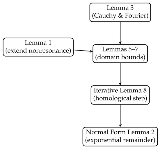
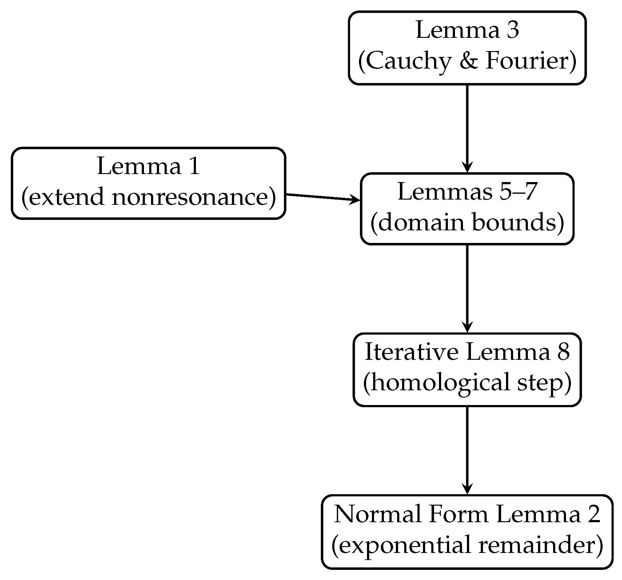
In order to transform the generating function $F(x,y)=F_0\left(x\right)+f(x,y)$ of $T_{\gamma }$ to the normal form, we need to seek a suitable canonical transformation $\Phi$, that is constructed iteratively as a product of the successive approximately identical canonical transformation ${\Phi }^{\left(1\right)},{\Phi }^{\left(2\right)},\dots$. In doing that, one meets the small denominators $1-e^{ik·\tilde{\omega }\left(x\right)}$, which in general vanish in a dense subset of ${\mathcal{G}}_{\gamma }$. These resonances are given by the equations $k·\tilde{\omega }\left(x\right)+2\pi l=0$, for $k\in {\mathbb{Z}}^n,l\in \mathbb{Z}$. As usual, the small denominators $1-e^{ik·\tilde{\omega }\left(x\right)}$ should be excluded in the process of constructing the normal form. However, it is not necessary to take care of all the small denominators. We can do that in a certain subdomain which can guarantee $|1-e^{ik·\tilde{\omega }\left(x\right)}|\ge \alpha$ for $\left|k\right|\le K$ and $k\notin \mathcal{M}$, where $\alpha$ and K are independent parameters and $\mathcal{M}$ is a given sublattice of ${\mathbb{Z}}^n$. The dependencies among these lemmas are illustrated in Figure 1.

Figure 1. Dependencies among lemmas in the analytic part.

Next we give the related notations in detail. Let $\mathcal{M}$ be a sublattice of ${\mathbb{Z}}^n$. We only consider the maximal ones that are not properly contained in any other sublattice of the same dimension. A maximal sublattice $\mathcal{M}$ with dim $\mathcal{M}=r$ is called a K-lattice if it admits a basis $(k^{\left(1\right)},\dots ,k^{\left(r\right)})$ satisfying $|k^{\left(j\right)}{|}_1\le K$ for $j\le r$, and such a basis will be called a K-basis [32]. A function $g(x,y)$ is said to be in a normal form with respect to $\mathcal{M}$ of degree K if its Fourier series expansion in the angular variables is restricted to the form $g(x,y)={\sum }_{k\in {\mathcal{M},\left|k\right|}_1\le K}{g}_k\left(x\right)e^{ik·y}$. We express this by writing $g\in \mathcal{R}(\mathcal{M},K)$. Note that a function is in the normal form with respect to the trivial modulo $\mathcal{M}=0$ if it does not depend on the angular variables.

We restrict ourselves to a subset $G\subset {\mathcal{G}}_{\gamma }$, where the frequency vector $\tilde{\omega }\left(x\right)$ is allowed to satisfy some resonance relations corresponding to a fixed sublattice $\mathcal{M}$, but a neighborhood of all other resonances of order less than or equal to K are excluded. More precisely, a subset $G\subset {\mathcal{G}}_{\gamma }$ is said to be $\alpha ,K$-nonresonant modulo $\mathcal{M}$ if

$$|1-e^{ik·\tilde{\omega }\left(x\right)}|\ge \alpha forallk\in {\mathbb{Z}}_K^n\setminus \mathcal{M}andx\in G,$$

where ${\mathbb{Z}}_K^n:=\{k\in {\mathbb{Z}}^n{\left|\right|k|}_1\le K\}$.

A special situation arises when $\mathcal{M}$ is the trivial sublattice $\Theta$ of ${\mathbb{Z}}^n$ containing only 0. In this case, the set G is said to be completely $\alpha ,K$-nonresonant. In the corresponding normal form, g is independent of the angle variables. Naturally, the analysis of this case is simpler than the ones in the case of resonances.

The nonresonance condition on the set G can be extended to a complex neighborhood of small enough radius ${\rho }_1$.

Lemma 1. 

Let $F_0\left(x\right)$ be a real analytic function in ${\mathcal{V}}_{{\rho }_1}\left(G\right)$, and let $\tilde{\omega }=\partial F_0$. Assume that G is $\alpha ,K$-nonresonant modulo $\mathcal{M}$$(0<\alpha \le 1)$ and that $\tilde{\omega }$ satisfies (4). If

$${\rho }_1\le {\displaystyle \frac{\alpha }{4K\beta }},$$

then ${\mathcal{V}}_{{\rho }_1}\left(G\right)$ is $\alpha /2,K$-nonresonant modulo $\mathcal{M}$.

Proof. 

$\forall x\in {\mathcal{V}}_{{\rho }_1}\left(G\right)$, there exists $\tilde{x}\in G$ such that $|x-\tilde{x}{|}_2\le {\rho }_1$ by definition. Because

$$|1-e^{ik·\tilde{\omega }\left(x\right)}|\ge |1-e^{ik·\tilde{\omega }\left(\tilde{x}\right)}|-|e^{ik·\tilde{\omega }\left(x\right)}-e^{ik·\tilde{\omega }\left(\tilde{x}\right)}|\ge \alpha -|e^{ik·\tilde{\omega }\left(x\right)}-e^{ik·\tilde{\omega }\left(\tilde{x}\right)}|$$

to rigorously estimate the difference in the complex domain, we use the integral representation along the line segment connecting $\tilde{\omega }\left(\tilde{x}\right)$ and $\tilde{\omega }\left(x\right)$:

$$e^{ik·\tilde{\omega }\left(x\right)}-e^{ik·\tilde{\omega }\left(\tilde{x}\right)}={\int }_0^1{e}^{ik·[\tilde{\omega }\left(\tilde{x}\right)+t(\tilde{\omega }\left(x\right)-\tilde{\omega }\left(\tilde{x}\right))]}⟨ik,\tilde{\omega }\left(x\right)-\tilde{\omega }\left(\tilde{x}\right)⟩dt.$$

Let ${\omega }_t=\tilde{\omega }\left(\tilde{x}\right)+t(\tilde{\omega }\left(x\right)-\tilde{\omega }\left(\tilde{x}\right))$. Since $\tilde{x}\in G\subset {\mathbb{R}}^n$, $\tilde{\omega }\left(\tilde{x}\right)$ is purely real, which implies that $\mathtt{Im}{\omega }_t=t\mathtt{Im}\tilde{\omega }\left(x\right)$. Noting that the complex conjugation $\overline{x}$ satisfies $|\overline{x}-\tilde{x}{|}_2={|x-\tilde{x}|}_2\le {\rho }_1$, we have $|x-\overline{x}{|}_2\le 2{\rho }_1$. By the Lipschitz condition in (4),

$$|\mathtt{Im}\tilde{\omega }{\left(x\right)|}_2={\displaystyle \frac{1}{2}}|\tilde{\omega }\left(x\right)-\tilde{\omega }\left(\overline{x}\right){|}_2\le {\displaystyle \frac{1}{2}}\beta {|x-\overline{x}|}_2\le \beta {\rho }_1$$

Therefore, for any $t\in [0,1]$,

$$\left|e^{ik·{\omega }_t}\right|\le e^{{\left|k\right|}_1{\left|\mathtt{Im}{\omega }_t\right|}_{\infty }}\le e^{K|\mathtt{Im}\tilde{\omega }{\left(x\right)|}_2}\le e^{K\beta {\rho }_1}\le e^{1/4}\le 2,$$

where we used the assumption ${\rho }_1\le {\displaystyle \frac{\alpha }{4K\beta }}$ and $\alpha \le 1$. Bounding the integral, we obtain

$$|e^{ik·\tilde{\omega }\left(x\right)}-e^{ik·\tilde{\omega }\left(\tilde{x}\right)}|\le \underset{t\in [0,1]}{sup}|e^{ik·{\omega }_t}|·{\left|k\right|}_1·{|\tilde{\omega }\left(x\right)-\tilde{\omega }\left(\tilde{x}\right)|}_2\le 2K\beta {\rho }_1\le {\displaystyle \frac{\alpha }{2}}.$$

That completes the proof. □

The Normal Form Lemma can be formulated as follows.

Lemma 2 

(Normal Form Lemma). Let $\mathcal{M}\subseteq {\mathbb{Z}}^n$ be a K-lattice, $0<\alpha \le 1$ and $\beta \le \alpha$. $F(x,y)=F_0\left(x\right)+f(x,y)$ is analytic in ${\mathcal{D}}_{\rho }\left(G\right)$, $\rho =({\rho }_1,{\rho }_2)$. Suppose that ${\mathcal{V}}_{{\rho }_1}\left(G\right)$ is $\alpha ,K$-nonresonant modulo $\mathcal{M}$ and the frequency map $\tilde{\omega }$ satisfies (4). If

$${\left|\right|Df\left|\right|}_{G,\rho ,c}\le {\displaystyle \frac{\alpha {\rho }_1}{\tilde{C}AK{\rho }_2}},$$

(5)

where $\tilde{C}=21n+30,A=1+{\displaystyle \frac{\beta c}{\alpha }}{e}^{K\beta {\rho }_1}$ and ${\rho }_1\le min({\displaystyle \frac{\alpha }{4K\beta }},1)$, then there exists a real analytic canonical transformation $\Phi :{\mathcal{D}}_{{\displaystyle \frac{\rho }{2}}}\left(G\right)\to {\mathcal{D}}_{\rho }\left(G\right)$ such that the conjugate symplectic map $T_{\gamma }^{\prime }={\Phi }^{-1}\circ T_{\gamma }\circ \Phi :{\mathcal{D}}_{{\displaystyle \frac{\rho }{2}}}\left(G\right)\to {\mathcal{D}}_{\rho }\left(G\right)$ is generated by the analytic function $F^{\prime }=F_0+Z+R$ with $Z\in \mathcal{R}(\mathcal{M},K)$. Moreover, the following hold:

(1) 

${\left|\right|DZ\left|\right|}_{G,{\displaystyle \frac{\rho }{2}},c}\le {2\left|\right|Df\left|\right|}_{G,\rho ,c}$.

(2) 

${\left|\right|DR\left|\right|}_{G,{\displaystyle \frac{\rho }{2}},c}\le 3e^{-{\displaystyle \frac{K{\rho }_2}{12}}}{\left|\right|Df\left|\right|}_{G,\rho ,c}$.

(3) 

$|P_x{\Phi -id|}_{G,{\displaystyle \frac{\rho }{2}}}\le {\displaystyle \frac{{\rho }_1}{2^8}}$, where $P_x$ denotes the projection onto x-coordinates.

In order to prove the Normal Form Lemma, we need some technique lemmas.

Lemma 3 

([31]). Let f be an analytic function in ${\mathcal{D}}_{\rho }\left(G\right)$. For $0<\delta =({\delta }_1,{\delta }_2)<\rho$ and $c>0$ given, let us denote

$${\widehat{\delta }}_c:=min({\delta }_1,c{\delta }_2).$$

Then,

(a) 

${\left|\right|Df\left|\right|}_{G,\rho -\delta ,c}\le {\displaystyle \frac{c}{{\widehat{\delta }}_c}}{\left|\right|f\left|\right|}_{G,\rho }.$

(b) 

$\left|\right|D\left(f^{>K}\right){\left|\right|}_{G,\rho -\delta ,c}\le e^{-K{\delta }_2}{\left|\right|Df\left|\right|}_{G,\rho ,c},$ where $f^{>K}(x,y)={\displaystyle \sum _{{\left|k\right|}_1>K}}{f}_k\left(x\right)e^{ik·y}$.

The following lemma is similar to Lemma 6 in [28], and the proof can be found there.

Lemma 4 

([28]). Let $T_{\gamma }$ and Φ be symplectic maps generated by analytic functions F and χ respectively. $T_{\gamma },\Phi :G\times {\mathbb{T}}^n\to G\times {\mathbb{T}}^n$ are defined by

$$\begin{array}{c}\Phi :(a,\phi )\to (x,y)\\ \left\{\begin{array}{cc}\hfill x& =a+{\partial }_2\chi (a,y)\hfill \\ \hfill y& =\phi -{\partial }_1\chi (a,y)\hfill \end{array}\right.\end{array}$$

(6)

and

$$\begin{array}{c}{T}_{\gamma }:(x,y)\to (\widehat{x},\widehat{y})\\ \left\{\begin{array}{cc}\hfill \widehat{x}& =x-{\partial }_{2}F(\widehat{x},y)\hfill \\ \hfill \widehat{y}& =y+{\partial }_{1}F(\widehat{x},y)\hfill \end{array}\right.\end{array}$$

(7)

Then one of the generating functions of the conjugate symplectic map $T_{\gamma }^{\prime }={\Phi }^{-1}\circ T_{\gamma }\circ \Phi :(a,\phi )\to (\widehat{a},\widehat{\phi })$ can be written as

$$\tilde{F}(\widehat{a},\phi )=a·\phi -a·y+\widehat{a}·\widehat{y}-\widehat{a}·\phi +\widehat{x}·y-\widehat{x}·\widehat{y}+F(\widehat{x},y)+\chi (\widehat{a},\widehat{y})-\chi (a,y),$$

where $x,\widehat{x},y,\widehat{y},a,\widehat{\phi }$ are functions of the independent variables $\widehat{a},\phi$.

Lemma 5. 

Let $\chi (x,y)$ be analytic in ${\mathcal{D}}_{\rho }\left(G\right)$, and given positive numbers $\delta =({\delta }_1,{\delta }_2)<({\rho }_1,{\rho }_2)$. Assume that ${\left|\right|D\chi \left|\right|}_{G,\rho ,c}\le {\displaystyle \frac{{\widehat{\delta }}_c}{2}}$; then the symplectic transformation Φ generated by the function χ is well defined in ${\mathcal{D}}_{\rho -\delta }\left(G\right)$. Furthermore, one has

$$\Phi \left({\mathcal{D}}_{\rho -\delta }\left(G\right)\right)\subseteq {\mathcal{D}}_{\rho -{\displaystyle \frac{\delta }{2}}}\left(G\right)and{\Phi }^{-1}\left({\mathcal{D}}_{\rho -\delta }\left(G\right)\right)\subseteq {\mathcal{D}}_{\rho -{\displaystyle \frac{\delta }{2}}}\left(G\right).$$

Proof. 

Let ${\mathcal{A}}_{{\delta }_1,{\delta }_2}=\{v:{\mathcal{D}}_{\rho -\delta }\left(G\right)\to {\mathbb{C}}^n{\left|\right|\left|v\right||}_{G,\rho -\delta }\le {\displaystyle \frac{{\delta }_2}{2}}\}$. It is easy to know that ${\mathcal{A}}_{{\delta }_1,{\delta }_2}$ is a closed-bounded subset of a Banach space. Now consider the map $\mathcal{F}\left(v\right)(x,y)={\displaystyle \frac{\partial \chi (x,y-v(x,y\left)\right)}{\partial x}}$, which is well defined for any $v\in {\mathcal{A}}_{{\delta }_1,{\delta }_2}$ and maps the space into itself from the fact that

$${\left|\right|\mathcal{F}\left|\right|}_{G,\rho -\delta }\le {\displaystyle \frac{1}{c}}{\left|\right|D\chi \left|\right|}_{G,\rho ,c}\le {\displaystyle \frac{{\widehat{\delta }}_c}{2c}}\le {\displaystyle \frac{{\delta }_2}{2}}.$$

(8)

Moreover, for any $v_1,v_2\in {\mathcal{A}}_{{\delta }_1,{\delta }_2}$, one has

$$\begin{array}{cc}\hfill \left|\right|\mathcal{F}\left(v_1\right)(x,y)-\mathcal{F}\left(v_2\right)(x,y){\left|\right|}_{G,\rho -\delta }& =\left|\right|{\displaystyle \frac{\partial \chi (x,y-v_1(x,y))}{\partial x}}-{\displaystyle \frac{\partial \chi (x,y-v_2(x,y))}{\partial x}}|{|}_{G,\rho -\delta }\hfill \\ \hfill & =\left|\right|{\displaystyle \frac{{\partial }^2\chi (x,y^{*})}{\partial x\partial y}}·(v_1-v_2)|{|}_{G,\rho -\delta }\hfill \\ \hfill & \le {\displaystyle \frac{1}{{\delta }_1}}\left|\right|{\displaystyle \frac{\partial \chi }{\partial y}}|{|}_{G,\rho ,1}·\left|\right|v_1-v_2{\left|\right|}_{G,\rho -\delta }\hfill \\ \hfill & \le {\displaystyle \frac{1}{2}}\left|\right|v_1-v_2{\left|\right|}_{G,\rho -\delta }.\hfill \end{array}$$

This shows that the map $\mathcal{F}:{\mathcal{A}}_{{\delta }_1,{\delta }_2}\to {\mathcal{A}}_{{\delta }_1,{\delta }_2}$ is contractive. Therefore, there exists a unique $v^{*}\in {\mathcal{A}}_{{\delta }_1,{\delta }_2}$ such that $\mathcal{F}\left(v^{*}\right)=v^{*}$ and the symplectic transformation $\Phi :(x,y)\to (\widehat{x},\widehat{y})$ can be expressed explicitly in the form

$$\left\{\begin{array}{cc}\hfill \widehat{x}& =x+{\displaystyle \frac{\partial \chi (x,y-v^{*})}{\partial y}}\hfill \\ \hfill \widehat{y}& =y-{\displaystyle \frac{\partial \chi (x,y-v^{*})}{\partial x}}\hfill \end{array}\right.$$

which is well defined and real analytic for any $(x,y)\in {\mathcal{D}}_{\rho -\delta }\left(G\right)$. It is easy to show $\Phi \left({\mathcal{D}}_{\rho -\delta }\left(G\right)\right)\subseteq {\mathcal{D}}_{\rho -{\displaystyle \frac{\delta }{2}}}\left(G\right)$ by means of (8) and

$$\left|\right|{\displaystyle \frac{\partial \chi (x,y-v^{*})}{\partial y}}|{|}_{G,\rho -\delta ,1}\le {\left|\right|D\chi \left|\right|}_{G,\rho ,c}\le {\displaystyle \frac{{\delta }_1}{2}}.$$

In similar way, we can prove that ${\Phi }^{-1}\left({\mathcal{D}}_{\rho -\delta }\left(G\right)\right)\subseteq {\mathcal{D}}_{\rho -{\displaystyle \frac{\delta }{2}}}\left(G\right)$. Specifically, we denote the set ${\tilde{\mathcal{A}}}_{{\delta }_1,{\delta }_2}=\{u:{\mathcal{D}}_{\rho -\delta }\left(G\right)\to {\mathbb{C}}^n{\left|\right|\left|u\right||}_{G,\rho -\delta }\le {\displaystyle \frac{{\delta }_2}{2}}\}$ and consider the map $\tilde{\mathcal{F}}\left(u\right)(x,y)={\displaystyle \frac{\partial \chi (x+u(x,y),y)}{\partial y}}$, which is well defined in ${\tilde{\mathcal{A}}}_{{\delta }_1,{\delta }_2}$. □

Lemma 6. 

Let $F(\widehat{x},y)=F_0\left(\widehat{x}\right)+f(\widehat{x},y)$ be analytic in ${\mathcal{D}}_{\rho }\left(G\right)$, with $\tilde{\omega }\left(x\right)=\partial F_0\left(x\right)$ satisfying (4). Given positive numbers $\delta =({\delta }_1,{\delta }_2)<({\rho }_1,{\rho }_2)$, if

$${\rho }_1\le {\displaystyle \frac{{\delta }_2}{6\beta }}{and\left|\right|Df\left|\right|}_{G,\rho ,c}\le {\displaystyle \frac{{\widehat{\delta }}_c}{2}},$$

then the symplectic map $T_{\gamma }$ generated by F is well defined in ${\mathcal{D}}_{\rho -\delta }\left(G\right)$ and

$$T_{\gamma }\left({\mathcal{D}}_{\rho -\delta }\left(G\right)\right)\subseteq {\mathcal{D}}_{{\rho }_1-{\displaystyle \frac{{\delta }_1}{2}},{\rho }_2-{\displaystyle \frac{{\delta }_2}{3}}}\left(G\right),T_{\gamma }^{-1}\left({\mathcal{D}}_{\rho -\delta }\left(G\right)\right)\subseteq {\mathcal{D}}_{{\rho }_1-{\displaystyle \frac{{\delta }_1}{2}},{\rho }_2-{\displaystyle \frac{{\delta }_2}{3}}}\left(G\right).$$

Proof. 

Similar to the proof of Lemma 5, for any $(x,y)\in {\mathcal{D}}_{\rho -\delta }\left(G\right)$, there exists a unique $\widehat{x}\in {\mathcal{V}}_{{\rho }_1-{\displaystyle \frac{{\delta }_1}{2}}}\left(G\right)$ such that $\widehat{x}=x-{\displaystyle \frac{\partial f(\widehat{x},y)}{\partial y}}$. Therefore, $\widehat{y}=y+\tilde{\omega }\left(\widehat{x}\right)+{\displaystyle \frac{\partial f(\widehat{x},y)}{\partial \widehat{x}}}$ is also well defined in ${\mathcal{D}}_{\rho -\delta }\left(G\right)$. Moreover, when $(x,y)\in {\mathcal{D}}_{\rho -\delta }\left(G\right)$,

$$\begin{array}{cc}\hfill |\mathtt{Im}(\widehat{y}-y){|}_{\infty }& \le |\mathtt{Im}\tilde{\omega }\left(\widehat{x}\right){|}_{G,{\rho }_1-{\delta }_1/2,\infty }+\left|\right|{\displaystyle \frac{\partial f}{\partial x}}|{|}_{G,\rho ,\infty }\hfill \\ \hfill & \le |{\displaystyle \frac{\tilde{\omega }\left(\widehat{x}\right)-\tilde{\omega }\left(\overline{\widehat{x}}\right)}{2}}{|}_{G,{\rho }_1-{\delta }_1/2,\infty }+{\displaystyle \frac{1}{c}}{\left|\right|Df\left|\right|}_{G,\rho ,c}\hfill \\ \hfill & \le {\displaystyle \frac{\beta }{2}}{|\widehat{x}-\overline{\widehat{x}}|}_2+{\displaystyle \frac{{\delta }_2}{2}}.\hfill \end{array}$$

Considering $\widehat{x}\in {\mathcal{V}}_{{\rho }_1-{\displaystyle \frac{{\delta }_1}{2}}}\left(G\right)$, there exists $x^{\prime }\in G$ such that $|\widehat{x}-x^{\prime }{|}_2\le {\rho }_1$. Thus

$$|\widehat{x}-\overline{\widehat{x}}{|}_2\le |\widehat{x}-x^{\prime }{|}_2+{|\overline{x^{\prime }}-\overline{\widehat{x}}|}_2\le 2{\rho }_1\le {\displaystyle \frac{{\delta }_2}{3\beta }}.$$

Therefore, $|\mathtt{Im}(\widehat{y}-y){|}_{\infty }\le {\displaystyle \frac{2}{3}}{\delta }_2,$ and we get

$$T_{\gamma }\left({\mathcal{D}}_{\rho -\delta }\left(G\right)\right)\subseteq {\mathcal{D}}_{{\rho }_1-{\displaystyle \frac{{\delta }_1}{2}},{\rho }_2-{\displaystyle \frac{{\delta }_2}{3}}}\left(G\right).$$

In similar way, one can prove that $T_{\gamma }^{-1}\left({\mathcal{D}}_{\rho -\delta }\left(G\right)\right)\subseteq {\mathcal{D}}_{{\rho }_1-{\displaystyle \frac{{\delta }_1}{2}},{\rho }_2-{\displaystyle \frac{{\delta }_2}{3}}}\left(G\right)$. □

Using Lemmas 4–6, we can derive the following lemma.

Lemma 7. 

Consider the generating function $F(\widehat{x},y)=F_0\left(\widehat{x}\right)+f(\widehat{x},y)$ and χ, which are analytic in ${\mathcal{D}}_{\rho }\left(G\right)$. Let $\tilde{\omega }\left(x\right)=\partial F_0\left(x\right)$ satisfy (4). Positive numbers $\delta =({\delta }_1,{\delta }_2)$ are given such that $3\delta \le \rho$. Suppose that

$${\rho }_1\le {\displaystyle \frac{{\delta }_2}{6\beta }}{,\left|\right|Df\left|\right|}_{G,\rho ,c}\le {\displaystyle \frac{{\widehat{\delta }}_c}{2}}{and\left|\right|D\chi \left|\right|}_{G,\rho ,c}\le {\displaystyle \frac{{\widehat{\delta }}_c}{2}}.$$

Let $T_{\gamma }$ be the symplectic map generated by F, Φ by χ and $T_{\gamma }^{\prime }={\Phi }^{-1}\circ T_{\gamma }\circ \Phi$. Then $T_{\gamma }^{\prime }$ and ${T_{\gamma }^{\prime }}^{-1}$ are analytic and symplectic diffemorphisms which are defined in ${\mathcal{D}}_{{\rho }_1-2{\delta }_1,{\rho }_2-3{\delta }_2}\left(G\right)$.

$$T_{\gamma }^{\prime }\left({\mathcal{D}}_{{\rho }_1-2{\delta }_1,{\rho }_2-3{\delta }_2}\left(G\right)\right)\subseteq {\mathcal{D}}_{{\rho }_1-{\displaystyle \frac{{\delta }_1}{2}},{\rho }_2-{\displaystyle \frac{4}{3}}{\delta }_2}\left(G\right),$$

and

$${T_{\gamma }^{\prime }}^{-1}\left({\mathcal{D}}_{{\rho }_1-2{\delta }_1,{\rho }_2-3{\delta }_2}\left(G\right)\right)\subseteq {\mathcal{D}}_{{\rho }_1-{\displaystyle \frac{{\delta }_1}{2}},{\rho }_2-{\displaystyle \frac{4}{3}}{\delta }_2}\left(G\right).$$

In addition, the conjugate symplectic map $T_{\gamma }^{\prime }$ can be generated by a function $\tilde{F}$, which is analytic in a domain containing ${\mathcal{D}}_{\rho -3\delta }\left(G\right)$.

Next, we formulate and prove the Iterative Lemma that is crucial in the proof of the Normal Form Lemma.

Lemma 8 

(Iterative Lemma). Consider that $F(\widehat{x},y)=F_0\left(\widehat{x}\right)+Z(\widehat{x},y)+R(\widehat{x},y)$, real analytic in ${\mathcal{D}}_{\rho }\left(G\right)$ and ${\mathcal{V}}_{{\rho }_1}\left(G\right)$, is $\alpha ,K$-nonresonance modulo $\mathcal{M}$, $Z\in \mathcal{R}(\mathcal{M},K)$. Let the symplectic map $T_{\gamma }:(x,y)\to (\widehat{x},\widehat{y})$ be given by the generating function $F(\widehat{x},y)$, and let $\tilde{\omega }\left(x\right)=\partial F_0\left(x\right)$ satisfy condition (4) where $\beta \le \alpha$. Assume that

$${\left|\right|DZ\left|\right|}_{G,\rho ,c}+{\left|\right|DR\left|\right|}_{G,\rho ,c}\le {\displaystyle \frac{\alpha {\widehat{\delta }}_c}{4A}}with3\delta \le \rho ,{\rho }_1\le min\left({\displaystyle \frac{{\delta }_2}{6\beta }},1\right),$$

(9)

where $A=1+{\displaystyle \frac{\beta c}{\alpha }}{e}^{K\beta {\rho }_1}$. Then, there exists a real analytic canonical transformation $\Phi :(a,\phi )\to (x,y)$ such that the conjugate symplectic map $T_{\gamma }^{\prime }={\Phi }^{-1}\circ T_{\gamma }\circ \Phi$ is generated by $\tilde{F}(\widehat{a},\phi )=F_0\left(\widehat{a}\right)+\tilde{Z}(\widehat{a},\phi )+\tilde{R}(\widehat{a},\phi )$ with $\tilde{Z}\in \mathcal{R}(\mathcal{M},K)$, and $\tilde{F}$ is analytic in a domain containing ${\mathcal{D}}_{\rho -3\delta }\left(G\right)$. Furthermore, the following estimates can be derived:

(a)

$\left|\right|D\tilde{Z}{\left|\right|}_{G,\rho -3\delta ,c}\le {\left|\right|DZ\left|\right|}_{G,\rho ,c}+{\left|\right|DR\left|\right|}_{G,\rho ,c}.$

(b)

$\left|\right|D\tilde{R}{\left|\right|}_{G,\rho -3\delta ,c}\le \left\{{\displaystyle \frac{2}{{\delta }_1}}\left(1+{\displaystyle \frac{A}{\alpha }}\right)\left[{▵}_1{\left(\right|\left|DZ\right||}_{G,\rho ,c}+{\left|\right|DR\left|\right|}_{G,\rho ,c})+e^{-K{\delta }_2}\right]·{\left|\right|DR\left|\right|}_{G,\rho ,c}+{▵}_2{\left(\right|\left|DZ\right||}_{G,\rho ,c}+{\left|\right|DR\left|\right|}_{G,\rho ,c})+e^{-K{\delta }_2}+{\displaystyle \frac{2\beta AC}{\alpha }}\right\}·{\left|\right|DR\left|\right|}_{G,\rho ,c}$, where

$$\begin{array}{cc}\hfill {▵}_1& ={\displaystyle \frac{2A}{\alpha {\delta }_1}}+{\displaystyle \frac{2}{{\delta }_1}}+{\displaystyle \frac{A}{e\alpha {\delta }_2}}\left({\displaystyle \frac{\beta A}{\alpha }}+\beta +{\displaystyle \frac{2}{c}}\right),\hfill \\ \hfill {▵}_2& ={\displaystyle \frac{n+2}{{\delta }_1}}·{\displaystyle \frac{A}{\alpha }}+{\displaystyle \frac{n+1}{{\delta }_1}}+{\displaystyle \frac{nA}{e\alpha {\delta }_2}}\left({\displaystyle \frac{\beta A}{\alpha }}+\beta +{\displaystyle \frac{1}{c}}\right).\hfill \end{array}$$

(c)

$|P_x{\Phi -id|}_{G,\rho -3\delta }\le {\displaystyle \frac{A}{\alpha }}{\left|\right|DR\left|\right|}_{G,\rho ,c}.$

Proof. 

We define the transformation $\Phi :(a,\phi )\to (x,y)$ implicitly with the help of a undetermined generating function $\chi$ by

$$x=a+{\partial }_2\chi (a,y),y=\phi -{\partial }_1\chi (a,y).$$

According to Lemma 7, we have the generating function $\tilde{F}(\widehat{a},\phi )$ of the conjugate symplectic map $T_{\gamma }^{\prime }$, and $\tilde{F}$ is analytic in a domain containing ${\mathcal{D}}_{\rho -3\delta }\left(G\right)$.

We choose $\chi$ satisfying the linear functional equation

$$R^{\le K}+\chi (a,y+\tilde{\omega }\left(a\right))-\chi (a,y)=g(a,\phi )\mathrm{for} \mathrm{some}g\in \mathcal{R}(\mathcal{M},K),$$

where $R^{\le K}$ denotes the terms restricted to ${\left|k\right|}_1\le K$ in the Fourier expansion of R. By means of the Fourier expansions of R, $\chi$ and g, the solutions can be obtained:

$${\chi }_k\left(a\right)=\left\{\begin{array}{cc}{\displaystyle \frac{R_k\left(a\right)}{1-e^{ik·\tilde{\omega }\left(a\right)}}}\hfill & k\notin {\mathcal{M},\left|k\right|}_1\le K.\hfill \\ 0\hfill & \mathrm{else}.\hfill \end{array}\right.$$

and

$$g_k\left(a\right)=\left\{\begin{array}{cc}{R}_k\left(a\right)\hfill & k\in {\mathcal{M},\left|k\right|}_1\le K.\hfill \\ 0\hfill & \mathrm{else}.\hfill \end{array}\right.$$

Note that $\chi ={\sum }_{k\in {\mathbb{Z}}^n}{\chi }_k\left(a\right)e^{ik·y}$. Thus, $\chi (a,y)={\displaystyle \sum _{\begin{array}{c}k\notin \mathcal{M}\\ {\left|k\right|}_1\le K\end{array}}}{\displaystyle \frac{R_k\left(a\right)}{1-e^{ik·\tilde{\omega }\left(a\right)}}}·e^{ik·y},$ and

$$\left|\right|{\partial }_2{\chi \left|\right|}_{G,\rho ,1}=\sum _{\begin{array}{c}k\notin \mathcal{M}\\ {\left|k\right|}_1\le K\end{array}}|{\displaystyle \frac{k{R}_k\left(a\right)}{1-e^{ik·\tilde{\omega }\left(a\right)}}}{|}_{G,{\rho }_1,1}·e^{{\left|k\right|}_1·{\rho }_2}\le {\displaystyle \frac{1}{\alpha }}\left|\right|{\partial }_{2}R{\left|\right|}_{G,\rho ,1},$$

where in the last inequality, we use the nonresonance condition. Because

$$\partial {\chi }_k\left(a\right)={\displaystyle \frac{\partial R_k\left(a\right)}{1-e^{ik·\tilde{\omega }\left(a\right)}}}+{\displaystyle \frac{e^{ik·\tilde{\omega }\left(a\right)}{\left[{\partial }_{2}R\right]}_k\partial \tilde{\omega }}{{(1-e^{ik·\tilde{\omega }\left(a\right)})}^2}},fork\notin \mathcal{M},{\left|k\right|}_1\le K,$$

where we use the fact that ${\left[{\partial }_{2}R\right]}_k=i{R}_k\left(a\right)k$ (differentiating the Fourier expansion of R). As before, $|\mathtt{Im}\tilde{\omega }{\left(a\right)|}_{G,{\rho }_1,\infty }\le \beta {\rho }_1$. Thus

$$|\partial {\chi }_k{\left(a\right)|}_{G,{\rho }_1,\infty }\le {\displaystyle \frac{1}{\alpha }}|\partial R_k{\left(a\right)|}_{G,{\rho }_1,\infty }+{\displaystyle \frac{\beta }{{\alpha }^2}}{e}^{{\left|k\right|}_1\beta {\rho }_1}·{\left|{\left[{\partial }_{2}R\right]}_k\right|}_{G,{\rho }_1}.$$

Moreover,

$$\left|\right|{\partial }_1{\chi \left|\right|}_{G,\rho ,\infty }\le {\displaystyle \frac{1}{\alpha }}\left|\right|{\partial }_1{R|}_{G,\rho ,\infty }+{\displaystyle \frac{\beta }{{\alpha }^2}}{e}^{K\beta {\rho }_1}·\left|\right|{\partial }_{2}R{\left|\right|}_{G,\rho ,1}.$$

Therefore, we have

$$\begin{array}{cc}\hfill {\left|\right|D\chi \left|\right|}_{G,\rho ,c}& \le \left({\displaystyle \frac{1}{\alpha }}+{\displaystyle \frac{\beta c}{{\alpha }^2}}{e}^{K\beta {\rho }_1}\right)·{\left|\right|DR\left|\right|}_{G,\rho ,c}\hfill \\ \hfill & \triangleq {\displaystyle \frac{A}{\alpha }}{\left|\right|DR\left|\right|}_{G,\rho ,c}\hfill \end{array}$$

(10)

with $A=1+{\displaystyle \frac{\beta c}{\alpha }}{e}^{K\beta {\rho }_1}$.

Let $B=R_0^{-1}\circ {\Phi }^{-1}\circ T_{\gamma }\circ \Phi :(a,\phi )\to (\widehat{a},\widehat{\phi })$, where $R_0$ is an integrable rotation on $G\times {\mathbb{T}}^n$ with frequency map $\tilde{\omega }$, i.e., $R_0(a,\phi )=(a,\phi +\tilde{\omega }\left(a\right))$, and B can be expressed implicitly as follows:

$$\left\{\begin{array}{cc}\hfill \widehat{a}& =a+{\partial }_2\chi (a,y)-{\partial }_2\chi (\widehat{a},\widehat{y})-{\partial }_2(Z+R)(\widehat{x},y)\hfill \\ \hfill \widehat{\phi }& =\phi -{\partial }_1\chi (a,y)+{\partial }_1\chi (\widehat{a},\widehat{y})+{\partial }_1(Z+R)(\widehat{x},y)-\tilde{\omega }\left(\widehat{a}\right)+\tilde{\omega }\left(\widehat{x}\right).\hfill \end{array}\right.$$

(11)

On the other hand, let $\tilde{Z}(\widehat{a},\phi )=Z(\widehat{a},\phi )+{\mathcal{P}}_{\mathcal{M}}{\mathcal{T}}_{K}R(\widehat{a},\phi )$, where ${\mathcal{P}}_{\mathcal{M}}{\mathcal{T}}_{K}R$ denotes the terms restricted to $k\in \mathcal{M}$ and ${\left|k\right|}_1\le K$ in the Fourier expansion of R, and assume that the map ${\Phi }^{-1}\circ T_{\gamma }\circ \Phi$ has the form:

$$\left\{\begin{array}{cc}\hfill \widehat{a}& =a-{\partial }_2\tilde{Z}(\widehat{a},\phi )-{\partial }_2\tilde{R}(\widehat{a},\phi )\hfill \\ \hfill \widehat{\phi }& =\phi +\tilde{\omega }\left(\widehat{a}\right)+{\partial }_1\tilde{Z}(\widehat{a},\phi )+{\partial }_1\tilde{R}(\widehat{a},\phi ).\hfill \end{array}\right.$$

Then, B has the form:

$$\left\{\begin{array}{cc}\hfill \widehat{a}& =a-{\partial }_2\tilde{Z}(\widehat{a},\phi )-{\partial }_2\tilde{R}(\widehat{a},\phi )\hfill \\ \hfill \widehat{\phi }& =\phi +{\partial }_1\tilde{Z}(\widehat{a},\phi )+{\partial }_1\tilde{R}(\widehat{a},\phi ).\hfill \end{array}\right.$$

(12)

Combining (11) and (12), we have

$$\begin{array}{cc}\hfill \left|\right|{\partial }_2\tilde{R}(\widehat{a},\phi ){\left|\right|}_{G,\rho -3\delta ,1}& \le \left|\right|\widehat{a}-a+{\partial }_2\tilde{Z}(\widehat{a},\phi ){\left|\right|}_{G,\rho -\delta ,1}\hfill \\ \hfill & =\left|\right|{\partial }_2\chi (a,y)-{\partial }_2\chi (\widehat{a},\widehat{y})-{\partial }_2(Z+R)(\widehat{x},y)+{\partial }_2\tilde{Z}(\widehat{a},\phi ){\left|\right|}_{G,\rho -\delta ,1}\hfill \\ \hfill & \le I_1+I_2+I_3+I_4+I_5+I_6,\hfill \\ \hfill \left|\right|{\partial }_1\tilde{R}(\widehat{a},\phi ){\left|\right|}_{G,\rho -3\delta ,\infty }& \le \left|\right|\widehat{\phi }-\phi -{\partial }_1\tilde{Z}(\widehat{a},\phi ){\left|\right|}_{G,\rho -\delta ,\infty }\hfill \\ \hfill & =\left|\right|{\partial }_1\chi (\widehat{a},\widehat{y})-{\partial }_1\chi (a,y)+{\partial }_1(Z+R)(\widehat{x},y)-\tilde{\omega }\left(\widehat{a}\right)+\tilde{\omega }\left(\widehat{x}\right)\hfill \\ \hfill & -{\partial }_1\tilde{Z}(\widehat{a},\phi ){\left|\right|}_{G,\rho -\delta ,\infty }\hfill \\ \hfill & \le J_1+J_2+J_3+J_4+J_5+J_6+J_7.\hfill \end{array}$$

where

$$\begin{array}{cc}\hfill I_1& =\left|\right|{\partial }_2\chi (\widehat{a},\widehat{y})-{\partial }_2\chi (a,\widehat{y}){\left|\right|}_{G,\rho -\delta ,1},\hfill \\ \hfill I_2& =\left|\right|{\partial }_2\chi (a,\widehat{y})-{\partial }_2\chi (a,y+\tilde{\omega }\left(a\right)){\left|\right|}_{G,\rho -\delta ,1},\hfill \\ \hfill I_3& =\left|\right|{\partial }_2\chi (a,y+\tilde{\omega }\left(a\right))-{\partial }_2\chi (a,y)+{\partial }_2(R(a,y)-{\mathcal{P}}_{\mathcal{M}}{\mathcal{T}}_{K}R(a,y)){\left|\right|}_{G,\rho -\delta ,1},\hfill \\ \hfill I_4& =\left|\right|{\partial }_{2}R(\widehat{x},y)-{\partial }_{2}R(a,y){\left|\right|}_{G,\rho -\delta ,1},\hfill \\ \hfill I_5& =\left|\right|{\partial }_{2}Z(\widehat{x},y)-{\partial }_{2}Z(\widehat{a},y){\left|\right|}_{G,\rho -\delta ,1}+\left|\right|{\partial }_2{\mathcal{P}}_{\mathcal{M}}{\mathcal{T}}_{K}R(a,y)-{\partial }_2{\mathcal{P}}_{\mathcal{M}}{\mathcal{T}}_{K}R(\widehat{a},y){\left|\right|}_{G,\rho -\delta ,1},\hfill \\ \hfill I_6& =\left|\right|{\partial }_{2}Z(\widehat{a},y)-{\partial }_{2}Z(\widehat{a},\phi ){\left|\right|}_{G,\rho -\delta ,1}+\left|\right|{\partial }_2{\mathcal{P}}_{\mathcal{M}}{\mathcal{T}}_{K}R(\widehat{a},y)-{\partial }_2{\mathcal{P}}_{\mathcal{M}}{\mathcal{T}}_{K}R(\widehat{a},\phi ){\left|\right|}_{G,\rho -\delta ,1},\hfill \\ \hfill J_1& =\left|\right|{\partial }_1\chi (\widehat{a},\widehat{y})-{\partial }_1\chi (a,\widehat{y}){\left|\right|}_{G,\rho -\delta ,\infty },\hfill \\ \hfill J_2& =\left|\right|{\partial }_1\chi (a,\widehat{y})-{\partial }_1\chi (a,y+\tilde{\omega }\left(a\right)){\left|\right|}_{G,\rho -\delta ,\infty },\hfill \\ \hfill J_3& =\left|\right|{\partial }_1\chi (a,y+\tilde{\omega }\left(a\right))-{\partial }_1\chi (a,y)+\partial \tilde{\omega }\left(a\right){\partial }_2\chi (a,y+\tilde{\omega }\left(a\right))\hfill \\ \hfill & +{\partial }_1(R(a,y)-{\mathcal{P}}_{\mathcal{M}}{\mathcal{T}}_{K}R(a,y)){\left|\right|}_{G,\rho -\delta ,\infty },\hfill \\ \hfill J_4& =\left|\right|{\partial }_{1}R(\widehat{x},y)-{\partial }_{1}R(a,y){\left|\right|}_{G,\rho -\delta ,\infty },\hfill \\ \hfill J_5& =\left|\right|{\partial }_{1}Z(\widehat{x},y)-{\partial }_{1}Z(\widehat{a},y){\left|\right|}_{G,\rho -\delta ,\infty }+\left|\right|{\partial }_1{\mathcal{P}}_{\mathcal{M}}{\mathcal{T}}_K(R(a,y)-R(\widehat{a},y)){\left|\right|}_{G,\rho -\delta ,\infty },\hfill \\ \hfill J_6& =\left|\right|{\partial }_{1}Z(\widehat{a},y)-{\partial }_{1}Z(\widehat{a},\phi ){\left|\right|}_{G,\rho -\delta ,\infty }+\left|\right|{\partial }_1{\mathcal{P}}_{\mathcal{M}}{\mathcal{T}}_K(R(\widehat{a},y)-R(\widehat{a},\phi )){\left|\right|}_{G,\rho -\delta ,\infty },\hfill \\ \hfill J_7& =\left|\right|\tilde{\omega }\left(\widehat{x}\right)-\tilde{\omega }\left(\widehat{a}\right){\left|\right|}_{G,\rho -\delta ,\infty }+\left|\right|\partial \tilde{\omega }\left(a\right)·{\partial }_2\chi (a,y+\tilde{\omega }\left(a\right)){\left|\right|}_{G,\rho -\delta ,\infty }.\hfill \end{array}$$

Note that all the concerned variables are in ${\mathcal{D}}_{\rho -\delta }\left(G\right)$. By expressing the differences as integrals along line segments connecting the relevant points and applying Cauchy estimates, we are able to get the following bounds:

$$\begin{array}{cc}\hfill I_1& \le {\displaystyle \frac{1}{{\delta }_1}}\left|\right|{\partial }_2{\chi \left|\right|}_{G,\rho ,1}·\left|\right|\widehat{a}-a{\left|\right|}_{G,\rho -\delta ,1}\hfill \\ \hfill & \le {\displaystyle \frac{1}{{\delta }_1}}{\left|\right|D\chi \left|\right|}_{G,\rho ,c}·\left(\right||\widehat{a}-a+{\partial }_2\tilde{Z}(\widehat{a},\phi ){\left|\right|}_{G,\rho -\delta ,1}+\left|\right|{\partial }_2\tilde{Z}(\widehat{a},\phi ){\left|\right|}_{G,\rho -\delta ,1})\hfill \\ \hfill & \le {\displaystyle \frac{1}{{\delta }_1}}·{\displaystyle \frac{A}{\alpha }}{\left|\right|DR\left|\right|}_{G,\rho ,c}·\left(\right||\widehat{a}-a+{\partial }_2\tilde{Z}(\widehat{a},\phi ){\left|\right|}_{G,\rho -\delta ,1}+\left|\right|{\partial }_2\tilde{Z}(\widehat{a},\phi ){\left|\right|}_{G,\rho -\delta ,1}),\hfill \end{array}$$

where in the last inequality, we use (10).

$$\begin{array}{cc}\hfill I_2& \le {\displaystyle \frac{1}{e{\delta }_2}}\left|\right|{\partial }_2{\chi \left|\right|}_{G,\rho ,1}·\left|\right|\widehat{y}-y-\tilde{\omega }\left(a\right){\left|\right|}_{G,\rho -\delta ,\infty }\hfill \end{array}$$

$$\begin{array}{cc}\hfill & \le {\displaystyle \frac{1}{e{\delta }_2}}{\left|\right|D\chi \left|\right|}_{G,\rho ,c}·\left|\right|\widehat{y}-y-\tilde{\omega }\left(a\right){\left|\right|}_{G,\rho -\delta ,\infty }.\hfill \end{array}$$

Note that

$$\begin{array}{cc}\hfill \left|\right|\widehat{y}-y-\tilde{\omega }\left(a\right){\left|\right|}_{G,\rho -\delta ,\infty }& =\left|\right|\tilde{\omega }\left(\widehat{x}\right)-\tilde{\omega }\left(a\right)+{\partial }_1(Z+R)(\widehat{x},y){\left|\right|}_{G,\rho -\delta ,\infty }\hfill \\ \hfill & \le \beta ·\left|\right|\widehat{x}-{a\left|\right|}_{G,\rho -\delta ,1}+\left|\right|{\partial }_1(Z+R)(\widehat{x},y){\left|\right|}_{G,\rho -\delta ,\infty },\hfill \end{array}$$

and $\widehat{x}=a+{\partial }_2\chi (a,y)-{\partial }_2(Z+R)(\widehat{x},y)$, so

$$\left|\right|\widehat{x}-{a\left|\right|}_{G,\rho -\delta ,1}\le \left|\right|{\partial }_2{\chi \left|\right|}_{G,\rho -\delta ,1}+\left|\right|{\partial }_2(Z+R){\left|\right|}_{G,\rho -\delta ,1}.$$

Thus,

$$\left|\right|\widehat{y}-y-\tilde{\omega }{\left(a\right)\left|\right|}_{G,\rho -\delta ,\infty }\le {\beta \left(\right|\left|D\chi \right||}_{G,\rho -\delta ,c}+{\left|\right|D(Z+R)\left|\right|}_{G,\rho -\delta ,c})+{\displaystyle \frac{1}{c}}{\left|\right|D(Z+R)\left|\right|}_{G,\rho -\delta ,c}.$$

Therefore,

$$\begin{array}{cc}\hfill I_2& \le {\displaystyle \frac{A}{e\alpha {\delta }_2}}{\left|\right|DR\left|\right|}_{G,\rho ,c}·\left[{\displaystyle \frac{\beta A}{\alpha }}{\left|\right|DR\left|\right|}_{G,\rho ,c}+(\beta +{\displaystyle \frac{1}{c}})\left|\right|D(Z+R){\left|\right|}_{G,\rho ,c}\right].\hfill \end{array}$$

Similarly, we have

$$\begin{array}{cc}\hfill I_3& \le \left|\right|{\partial }_2{R}^{>K}{\left|\right|}_{G,\rho -\delta ,1}\le \left|\right|D{R}^{>K}{\left|\right|}_{G,\rho -\delta ,c}\le e^{-K{\delta }_2}{\left|\right|DR\left|\right|}_{G,\rho ,c},\hfill \end{array}$$

$$\begin{array}{cc}\hfill I_4& \le {\displaystyle \frac{1}{{\delta }_1}}\left|\right|{\partial }_2{R\left|\right|}_{G,\rho ,1}·\left|\right|\widehat{x}-{a\left|\right|}_{G,\rho -\delta ,1}\le {\displaystyle \frac{1}{{\delta }_1}}{\left|\right|DR\left|\right|}_{G,\rho ,c}·\left({\displaystyle \frac{A}{\alpha }}{\left|\right|DR\left|\right|}_{G,\rho ,c}+{\left|\right|D(Z+R)\left|\right|}_{G,\rho ,c}\right),\hfill \end{array}$$

$$\begin{array}{cc}\hfill I_5& \le {\displaystyle \frac{1}{{\delta }_1}}\left|\right|{\partial }_2{Z\left|\right|}_{G,\rho ,1}·\left|\right|\widehat{x}-\widehat{a}{\left|\right|}_{G,\rho -\delta ,1}+{\displaystyle \frac{1}{{\delta }_1}}\left|\right|{\partial }_2{R\left|\right|}_{G,\rho ,1}·\left|\right|\widehat{a}-a{\left|\right|}_{G,\rho -\delta ,1}\hfill \end{array}$$

$$\begin{array}{cc}\hfill & \le {\displaystyle \frac{1}{{\delta }_1}}{\left|\right|DZ\left|\right|}_{G,\rho ,c}·{\displaystyle \frac{A}{\alpha }}{\left|\right|DR\left|\right|}_{G,\rho ,c}+{\displaystyle \frac{1}{{\delta }_1}}{\left|\right|DR\left|\right|}_{G,\rho ,c}·\left(\left|\right|\widehat{a}-a+{\partial }_2\tilde{Z}{\left|\right|}_{G,\rho -\delta ,1}+\left|\right|{\partial }_2\tilde{Z}{\left|\right|}_{G,\rho ,1}\right),\hfill \end{array}$$

$$\begin{array}{cc}\hfill I_6& \le {\displaystyle \frac{1}{e{\delta }_2}}·{\displaystyle \frac{A}{c\alpha }}{\left|\right|DR\left|\right|}_{G,\rho ,c}·\left({\left|\right|DZ\left|\right|}_{G,\rho ,c}+{\left|\right|DR\left|\right|}_{G,\rho ,c}\right).\hfill \end{array}$$

By means of condition (9) and above estimates, we get

$$\begin{array}{cc}\hfill {\displaystyle \frac{1}{2}}\left|\right|\widehat{a}-a+{\partial }_2\tilde{Z}(\widehat{a},\phi ){\left|\right|}_{G,\rho -\delta ,1}\le & [\left({\displaystyle \frac{2A}{\alpha {\delta }_1}}+{\displaystyle \frac{2}{{\delta }_1}}+{\displaystyle \frac{A}{e\alpha {\delta }_2}}\left(\beta {\displaystyle \frac{A}{\alpha }}+\beta +{\displaystyle \frac{2}{c}}\right)\right)·{\left(\right|\left|DZ\right||}_{G,\rho ,c}\hfill \\ \hfill & +{\left|\right|DR\left|\right|}_{G,\rho ,c})+e^{-K{\delta }_2}]·{\left|\right|DR\left|\right|}_{G,\rho ,c}.\hfill \end{array}$$

Thus,

$$\left|\right|{\partial }_2\tilde{R}(\widehat{a},\phi ){\left|\right|}_{G,\rho -3\delta ,1}\le 2\left[{▵}_1·{\left(\right|\left|DR\right||}_{G,\rho ,c}+{\left|\right|DZ\left|\right|}_{G,\rho ,c})+e^{-K{\delta }_2}\right]·{\left|\right|DR\left|\right|}_{G,\rho ,c},$$

where ${▵}_1={\displaystyle \frac{2A}{\alpha {\delta }_1}}+{\displaystyle \frac{2}{{\delta }_1}}+{\displaystyle \frac{A}{e\alpha {\delta }_2}}({\displaystyle \frac{\beta A}{\alpha }}+\beta +{\displaystyle \frac{2}{c}}).$

By estimating $J_k,k=1,\dots ,7$ in a similar way to the above and making use of the previous estimates, we obtain

$$\begin{array}{cc}\hfill J_1& \le {\displaystyle \frac{1}{{\delta }_1}}\left|\right|{\partial }_1{\chi \left|\right|}_{G,\rho ,\infty }·\left|\right|\widehat{a}-a{\left|\right|}_{G,\rho -\delta ,1}\hfill \\ \hfill & \le {\displaystyle \frac{1}{c{\delta }_1}}·{\displaystyle \frac{A}{\alpha }}{\left|\right|DR\left|\right|}_{G,\rho ,c}·\left(\left|\right|\widehat{a}-a+{\partial }_2\tilde{Z}{\left|\right|}_{G,\rho -\delta ,1}+\left|\right|{\partial }_2\tilde{Z}{\left|\right|}_{G,\rho -\delta ,1}\right),\hfill \\ \hfill J_2& \le {\displaystyle \frac{1}{e{\delta }_2}}\left|\right|{\partial }_1{\chi \left|\right|}_{G,\rho }·\left|\right|\widehat{y}-y-\tilde{\omega }\left(a\right){\left|\right|}_{G,\rho -\delta ,\infty }\hfill \\ \hfill & \le {\displaystyle \frac{n}{e{\delta }_2}}·{\displaystyle \frac{A}{c\alpha }}{\left|\right|DR\left|\right|}_{G,\rho ,c}·\left({\displaystyle \frac{\beta A}{\alpha }}{\left|\right|DR\left|\right|}_{G,\rho ,c}+\left(\beta +{\displaystyle \frac{1}{c}}\right){\left|\right|D(Z+R)\left|\right|}_{G,\rho ,c}\right),\hfill \\ \hfill J_3& \le \left|\right|{\partial }_1{R}^{>K}{\left|\right|}_{G,\rho -\delta ,\infty }\le {\displaystyle \frac{1}{c}}\left|\right|D{R}^{>K}{\left|\right|}_{G,\rho -\delta ,c}\le {\displaystyle \frac{1}{c}}{e}^{-K{\delta }_2}{\left|\right|DR\left|\right|}_{G,\rho ,c},\hfill \\ \hfill J_4& \le {\displaystyle \frac{n}{c{\delta }_1}}{\left|\right|DR\left|\right|}_{G,\rho ,c}·\left({\displaystyle \frac{A}{\alpha }}{\left|\right|DR\left|\right|}_{G,\rho ,c}+{\left|\right|D(Z+R)\left|\right|}_{G,\rho ,c}\right),\hfill \\ \hfill J_5& \le {\displaystyle \frac{1}{c{\delta }_1}}{\left|\right|DZ\left|\right|}_{G,\rho ,c}·{\displaystyle \frac{A}{\alpha }}{\left|\right|DR\left|\right|}_{G,\rho ,c}+{\displaystyle \frac{1}{c{\delta }_1}}{\left|\right|DR\left|\right|}_{G,\rho ,c}·\left(\left|\right|\widehat{a}-a+{\partial }_2\tilde{Z}{\left|\right|}_{G,\rho -\delta ,1}+\left|\right|{\partial }_2\tilde{Z}{\left|\right|}_{G,\rho ,1}\right),\hfill \\ \hfill J_6& \le {\displaystyle \frac{1}{{\delta }_1}}·{\displaystyle \frac{A}{c\alpha }}{\left|\right|DR\left|\right|}_{G,\rho ,c}·\left({\left|\right|DZ\left|\right|}_{G,\rho ,c}+{\left|\right|DR\left|\right|}_{G,\rho ,c}\right),\hfill \\ \hfill J_7& \le 2\beta \left|\right|{\partial }_2{\chi \left|\right|}_{G,\rho -\delta ,1}\le 2\beta ·{\displaystyle \frac{A}{\alpha }}{\left|\right|DR\left|\right|}_{G,\rho ,c}.\hfill \end{array}$$

Combining the above estimates, we get

$$\begin{array}{cc}\hfill c\left|\right|{\partial }_1\tilde{R}(\widehat{a},\phi ){\left|\right|}_{G,\rho -3\delta ,\infty }\le & [{\displaystyle \frac{1}{{\delta }_1}}\left(1+{\displaystyle \frac{A}{\alpha }}\right)·\left|\right|\widehat{a}-a+{\partial }_2\tilde{Z}{\left|\right|}_{G,\rho -\delta ,1}+{▵}_2·\left({\left|\right|DZ\left|\right|}_{G,\rho ,c}+{\left|\right|DR\left|\right|}_{G,\rho ,c}\right)\hfill \\ \hfill & +e^{-K{\delta }_2}+{\displaystyle \frac{2\beta Ac}{\alpha }}]·{\left|\right|DR\left|\right|}_{G,\rho ,c},\hfill \end{array}$$

where

$${▵}_2={\displaystyle \frac{n+2}{{\delta }_1}}·{\displaystyle \frac{A}{\alpha }}+{\displaystyle \frac{n+1}{{\delta }_1}}+{\displaystyle \frac{nA}{e\alpha {\delta }_2}}\left({\displaystyle \frac{\beta A}{\alpha }}+\beta +{\displaystyle \frac{1}{c}}\right).$$

Because ${\delta }_1\le 1$, we have

$$\begin{array}{cc}\hfill {\left|\right|DR\left|\right|}_{G,\rho -3\delta ,c}& \le max\left(\left|\right|{\partial }_2\tilde{R}{\left|\right|}_{G,\rho -3\delta ,1},c\left|\right|{\partial }_1\tilde{R}{\left|\right|}_{G,\rho -3\delta ,\infty }\right)\hfill \\ \hfill & \le \{{\displaystyle \frac{2}{{\delta }_1}}\left(1+{\displaystyle \frac{A}{\alpha }}\right)\left[{▵}_1{\left(\right|\left|DZ\right||}_{G,\rho ,c}+{\left|\right|DR\left|\right|}_{G,\rho ,c})+e^{-K{\delta }_2}\right]·{\left|\right|DR\left|\right|}_{G,\rho ,c}\hfill \\ & +{▵}_2{\left(\right|\left|DZ\right||}_{G,\rho ,c}+{\left|\right|DR\left|\right|}_{G,\rho ,c})+e^{-K{\delta }_2}+{\displaystyle \frac{2\beta Ac}{\alpha }}\}·{\left|\right|DR\left|\right|}_{G,\rho ,c}.\hfill \end{array}$$

Finally,

$$|P_x{\Phi -id|}_{G,\rho -3\delta }\le \left|\right|{\partial }_2{\chi \left|\right|}_{G,\rho -\delta ,1}\le {\left|\right|D\chi \left|\right|}_{G,\rho ,c}\le {\displaystyle \frac{A}{\alpha }}{\left|\right|DR\left|\right|}_{G,\rho ,c}.$$

□

2.2. Proof of Normal Form Lemma

Adopting a process similar to Hamiltonian systems, we shall construct a series of symplectic transformations ${\Phi }^{\left(i\right)}$, each of which reduces the norm of the remainder by a factor ${\displaystyle \frac{1}{e}}$. After applying the Iterative Lemma N times, we can get an exponentially small remainder by choosing $N=N\left(K\right)$ adequately.

Let $N\ge 1$ be an integer to be chosen below. We denote ${\rho }^{\left(i\right)}=\rho -3i\delta$, with $\delta ={\displaystyle \frac{\rho }{6N}}$. Obviously, ${\rho }^{\left(i\right)}={\rho }^{(i-1)}-3\delta$.

Next we apply the Iterative Lemma N times and obtain a series of symplectic transformations ${\Phi }^{\left(i\right)}:{\mathcal{D}}_{{\rho }^{\left(i\right)}}\left(G\right)\to {\mathcal{D}}_{{\rho }^{(i-1)}}\left(G\right)$ for $1\le i\le N$. Let ${\Psi }^{\left(i\right)}={\Phi }^{\left(i\right)}\circ {\Phi }^{(i-1)}\circ \cdots \circ {\Phi }^{\left(1\right)}$, $T_{\gamma }^{\left(i\right)}={{\Psi }^{\left(i\right)}}^{-1}\circ T_{\gamma }\circ {\Psi }^{\left(i\right)}$ and the generating functions $F^{\left(i\right)}=F_0+Z^{\left(i\right)}+R^{\left(i\right)}$ of the symplectic map $T_{\gamma }^{\left(i\right)}$ with $Z^{\left(i\right)}\in \mathcal{R}(\mathcal{M},K)$.

Now, we are going to show that if ${\displaystyle \frac{K{\rho }_2}{6N}}\ge 2$, then the claims below are true for $1\le i\le N$:

(a)

$\left|\right|D{Z}^{\left(i\right)}{\left|\right|}_{G,{\rho }^{\left(i\right)},c}\le {\displaystyle \sum _{j=0}^{i-1}}\left|\right|D{R}^{\left(j\right)}{\left|\right|}_{G,{\rho }^{\left(j\right)},c}.$

(b)

$\left|\right|D{R}^{\left(i\right)}{\left|\right|}_{G,{\rho }^{\left(i\right)},c}\le {\displaystyle \frac{1}{e}}\left|\right|D{R}^{(i-1)}{\left|\right|}_{G,{\rho }^{(i-1)},c}.$

The proof is done by induction.

Setting $R^{\left(0\right)}=f$ and $Z^{\left(0\right)}=0$, we choose the parameter $c={\displaystyle \frac{{\rho }_1}{{\rho }_2}}={\displaystyle \frac{{\delta }_1}{{\delta }_2}}$ so that ${\widehat{\delta }}_c={\delta }_1=c{\delta }_2$. Due to ${\displaystyle \frac{1}{K}}\le {\displaystyle \frac{{\rho }_2}{12N}}$ and $\tilde{C}\ge 30$, we have

$${\left|\right|Df\left|\right|}_{G,\rho ,c}\le {\displaystyle \frac{\alpha {\rho }_1}{\tilde{C}AK{\rho }_2}}\le {\displaystyle \frac{\alpha {\rho }_1}{12\tilde{C}AN}}={\displaystyle \frac{\alpha {\delta }_1}{2\tilde{C}A}}\le {\displaystyle \frac{\alpha {\widehat{\delta }}_c}{60A}}.$$

Note that

$${\rho }_1\le {\displaystyle \frac{\alpha }{4K\beta }}\le {\displaystyle \frac{\alpha {\rho }_2}{48N\beta }}={\displaystyle \frac{\alpha {\delta }_2}{8\beta }}\le {\displaystyle \frac{{\delta }_2}{6\beta }},$$

Thus, the Iterative Lemma can be applied with ${\displaystyle \frac{\rho }{6N}}$ instead of $\delta$. Due to ${\rho }_1\le {\displaystyle \frac{\alpha }{4K\beta }}$, we have

$$A=1+{\displaystyle \frac{\beta c}{\alpha }}{e}^{K\beta {\rho }_1}\le 1+{\displaystyle \frac{2\beta c}{\alpha }}\le 1+{\displaystyle \frac{1}{2K{\rho }_2}}\le 2,$$

(13)

and

$${\displaystyle \frac{2\beta Ac}{\alpha }}\le {\displaystyle \frac{1}{K{\rho }_2}}\le {\displaystyle \frac{1}{12}}.$$

(14)

By means of (5) and (13), we get

$$\begin{array}{cc}\hfill \left|\right|D{R}^{\left(1\right)}{\left|\right|}_{G,{\rho }^{\left(1\right)},c}& \le \left({\displaystyle \frac{1}{e\tilde{C}}}+{\displaystyle \frac{n+2}{2\tilde{C}}}+{\displaystyle \frac{n+1}{2\tilde{C}}}+{\displaystyle \frac{n}{24e\tilde{C}}}+{\displaystyle \frac{1}{e^2}}+{\displaystyle \frac{1}{12}}\right)·{\left|\right|Df\left|\right|}_{G,\rho ,c}\hfill \\ \hfill & \le {\displaystyle \frac{1}{e}}{\left|\right|Df\left|\right|}_{G,\rho ,c}.\hfill \end{array}$$

Claim (a) is obviously true for $i=1$.

For $1<i\le N$, note that

$$\begin{array}{cc}\hfill \left|\right|D{R}^{(i-1)}{\left|\right|}_{G,{\rho }^{(i-1)},c}& \le {\displaystyle \frac{\left|\right|D{R}^{\left(0\right)}{\left|\right|}_{G,\rho ,c}}{e^{i-1}}}\le {\left|\right|Df\left|\right|}_{G,\rho ,c}\le {\displaystyle \frac{\alpha {\widehat{\delta }}_c}{60A}},\hfill \end{array}$$

and

$$\begin{array}{cc}\hfill \left|\right|D{Z}^{(i-1)}{\left|\right|}_{G,{\rho }^{(i-1)},c}& \le {\displaystyle \sum _{j=0}^{i-2}}\left|\right|D{R}^{\left(j\right)}{\left|\right|}_{G,{\rho }^{\left(j\right)},c}\le 2\left|\right|D{R}^{\left(0\right)}{\left|\right|}_{G,\rho ,c}\le {\displaystyle \frac{\alpha {\widehat{\delta }}_c}{30A}}.\hfill \end{array}$$

Thus, the Iterative Lemma can be applied with ${\displaystyle \frac{\rho }{6N}}$ instead of $\delta$. Claim (a) is easy to prove, and claim (b) can be proved by the following estimates:

$$\begin{array}{cc}\hfill \left|\right|D{R}^{\left(i\right)}{\left|\right|}_{G,{\rho }^{\left(i\right)},c}& \le \{{\displaystyle \frac{2}{{\delta }_1}}\left(1+{\displaystyle \frac{A}{\alpha }}\right)\left[{▵}_1\left(\left|\right|D{Z}^{(i-1)}{\left|\right|}_{G,{\rho }^{(i-1)},c}+\left|\right|D{R}^{(i-1)}{\left|\right|}_{G,{\rho }^{(i-1)},c}\right)+e^{-K{\delta }_2}\right]·\hfill \\ \hfill & \left|\right|D{R}^{(i-1)}{\left|\right|}_{G,{\rho }^{(i-1)},c}+{▵}_2\left(\left|\right|D{Z}^{(i-1)}{\left|\right|}_{G,{\rho }^{(i-1)},c}+\left|\right|D{R}^{(i-1)}{\left|\right|}_{G,{\rho }^{(i-1)},c}\right)\hfill \\ \hfill & +e^{-K{\delta }_2}+{\displaystyle \frac{2\beta AC}{\alpha }}\}·\left|\right|D{R}^{(i-1)}{\left|\right|}_{G,{\rho }^{(i-1)},c}\hfill \\ \hfill & \le \{{\displaystyle \frac{2}{{\delta }_1}}\left(1+{\displaystyle \frac{A}{\alpha }}\right)\left({▵}_1·{2\left|\right|Df\left|\right|}_{G,\rho ,c}+e^{-{\displaystyle \frac{K{\rho }_2}{6N}}}\right){\displaystyle \frac{{\left|\right|Df\left|\right|}_{G,\rho ,c}}{e}}+2{▵}_2{\left|\right|Df\left|\right|}_{G,\rho ,c}\hfill \\ \hfill & +e^{-{\displaystyle \frac{K{\rho }_2}{6N}}}+{\displaystyle \frac{1}{12}}\}·\left|\right|D{R}^{(i-1)}{\left|\right|}_{G,{\rho }^{(i-1)},c}\hfill \\ \hfill & \le {\displaystyle \frac{1}{e}}\left|\right|D{R}^{(i-1)}{\left|\right|}_{G,{\rho }^{(i-1)},c}.\hfill \end{array}$$

Now we may choose $N=\left[{\displaystyle \frac{K{\rho }_2}{12}}\right]$, the integer part of ${\displaystyle \frac{K{\rho }_2}{12}}$. After iterating N times, the exponential small remainder is given by

$${\left|\right|DR\left|\right|}_{G,{\displaystyle \frac{\rho }{2}},c}=\left|\right|D{R}^{\left(N\right)}{\left|\right|}_{G,{\displaystyle \frac{\rho }{2}},c}\le {\displaystyle \frac{{\left|\right|Df\left|\right|}_{G,\rho ,c}}{e^N}}\le 3e^{-{\displaystyle \frac{K{\rho }_2}{12}}}{\left|\right|Df\left|\right|}_{G,\rho ,c}.$$

Conclusion (3) is obtained from the fact that

$$\begin{array}{cc}\hfill |P_x{\Phi -id|}_{G,{\displaystyle \frac{\rho }{2}}}& \le {\displaystyle \sum _{i=1}^N}|P_x{\Phi }^{\left(i\right)}{-id|}_{G,{\rho }^i}\le {\displaystyle \sum _{i=1}^N}{\displaystyle \frac{A}{\alpha }}\left|\right|D{R}^{\left(i\right)}{\left|\right|}_{G,{\rho }^{\left(i\right)},c}\le {\displaystyle \frac{2A}{\alpha }}{\left|\right|Df\left|\right|}_{G,\rho ,c}\hfill \\ \hfill & \le {\displaystyle \frac{{\rho }_1}{2^8}},\hfill \end{array}$$

where the last inequality is a consequence of (5) and $\tilde{C}\ge 48$. Here we remark that if $K{\rho }_2\le 12$, all results are obvious if we take $\Phi$ as the identity map.

3. The Geometry of Resonances

This section concerns the covering of the whole action space ${\mathcal{G}}_{\gamma }$ by a family of resonant blocks associated to different lattices $\mathcal{M}$. For the symplectic map, the original geometric construction in [32] requires some modifications (see also [28]). Here in addition to K, our geometric construction will be characterized by $2n$ positive parameters $0<{\alpha }_0={\alpha }_1\le {\alpha }_2\le \cdots \le {\alpha }_n<1$ and ${\delta }_1,{\delta }_2,\cdots ,{\delta }_n$. More precisely, for any choice of these parameters, for each K-lattice $\mathcal{M}\subseteq {\mathbb{Z}}^n$ with dim $\mathcal{M}=r$ and some $l=(l_1,\dots ,l_r)\in {\mathbb{Z}}^r$, we define:

(i)

Resonant manifold:

$${\mathcal{R}}_{\mathcal{M}}^l=\left\{x\in {\mathcal{G}}_{\gamma };k^{\left(j\right)}·\tilde{\omega }\left(x\right)+2\pi l_j=0,j=1,\dots ,r\right\}.$$

where $k^{\left(1\right)},\dots ,k^{\left(r\right)}$ is a K-basis.

(ii)

Resonant zone:

$${\mathcal{Z}}_{\mathcal{M}}^l=\left\{x\in {\mathcal{G}}_{\gamma };|k^{\left(j\right)}·\tilde{\omega }\left(x\right)+2\pi l_j|\le {\alpha }_r,j=1,\dots ,r\right\}.$$

where $k^{\left(1\right)},\dots ,k^{\left(r\right)}$ is a K-basis.

(iii)

Resonant block:

$${\mathcal{B}}_{\mathcal{M}}^l={\mathcal{Z}}_{\mathcal{M}}^l\setminus {\mathcal{Z}}_{r+1}^{*}.$$

Specifically, ${\mathcal{B}}_0={\mathcal{Z}}_0\setminus {\mathcal{Z}}_1^{*}$. The dimension r of $\mathcal{M}$ will also be called the multiplicity of the corresponding resonant manifold, zone or block.

(iv)

Cylinder:

First, let ${\Pi }_{\mathcal{M}}\left(x\right)$ be the hyperplane through x parallel to $\mathcal{M}$ with the same dimensionality, and denote its ${\delta }_r$ neighborhood by ${\Pi }_{\mathcal{M},{\delta }_r}\left(x\right)$, i.e.,

$${\Pi }_{\mathcal{M},{\delta }_r}\left(x\right)=\left\{\tilde{x}\in {\mathbb{R}}^n;\mathrm{dist}(\tilde{x},{\Pi }_{\mathcal{M}}\left(x\right))\le {\delta }_r\right\}.$$

Then, for $x\in {\mathcal{B}}_{\mathcal{M}}^l$, the cylinder is defined by

$${\mathcal{C}}_{\mathcal{M},{\delta }_r}^l\left(x\right)={\Pi }_{\mathcal{M},{\delta }_r}\left(x\right)\bigcap {\mathcal{Z}}_{\mathcal{M}}^l,$$

and the set ${\Pi }_{\mathcal{M},{\delta }_r}\left(x\right)\bigcap \partial {\mathcal{Z}}_{\mathcal{M}}$ gives the cylinder lateral walls.

(v)

Extended resonant block:

$${\mathcal{B}}_{\mathcal{M},{\delta }_r}^l=\bigcup _{x\in {\mathcal{B}}_{\mathcal{M}}^l}{\mathcal{C}}_{\mathcal{M},{\delta }_r}^l\left(x\right).$$

Remark 3. 

In the definition of the resonant zone, we make the point that l is bounded because of ${\left|k\right|}_1\le K$ and the boundedness of $\tilde{\omega }\left(x\right)$ and α. In addition, the resonant zones with the same lattice $\mathcal{M}$ do not intersect for different l.

Remark 4. 

The resonant blocks ${\mathcal{B}}_{\mathcal{M}}^l$ constitute a covering of the action space ${\mathcal{G}}_{\gamma }$, that is, ${\mathcal{G}}_{\gamma }={\bigcup }_l{\bigcup }_{\mathcal{M}}{\mathcal{B}}_{\mathcal{M}}^l.$

Now, we shall prove some properties of the geometry construction.

Proposition 1. 

(i) For any $x\in {\mathcal{B}}_{\mathcal{M}}^l$ with dim$\left(\mathcal{M}\right)=r\in \{0,1,\dots ,n-1\}$, if $k\in {\mathbb{Z}}_K^n\setminus \mathcal{M}$, then $|k·\tilde{\omega }\left(x\right)+2\pi l_0|>{\alpha }_{r+1}$ for any $l_0\in \mathbb{Z}$. In particular, for any $x\in {\mathcal{B}}_0$, $|k·\tilde{\omega }\left(x\right)+2\pi l_0|>{\alpha }_1$ for any $k\in {\mathbb{Z}}_K^n\setminus \left\{0\right\},l_0\in \mathbb{Z}$.

(ii)

$$\bigcup _l\bigcup _{\dim \left(\mathcal{M}\right)=r}{\mathcal{B}}_{\mathcal{M}}^l={\mathcal{Z}}_r^{*}\setminus {\mathcal{Z}}_{r+1}^{*}.$$

(iii)

$${\mathcal{G}}_{\gamma }\setminus {\mathcal{Z}}_{r+1}^{*}=\bigcup _l\bigcup _{\dim \left(\mathcal{M}\right)\le r}{\mathcal{B}}_{\mathcal{M}}^l.$$

(iv) If $\mathcal{M}$ is an r-dimensional K-lattice, $1\le r\le n$, then for any $x\in {\mathcal{B}}_{\mathcal{M}}^l$,

$$\mathrm{diam}\left({\mathcal{C}}_{\mathcal{M},{\delta }_r}^l\left(x\right)\right)\le {\displaystyle \frac{4}{\mu }}{\delta }_r+{\displaystyle \frac{2r{K}^{r-1}}{\beta \mu }}{\alpha }_r.$$

Proof. 

In order to prove statement (i) by contradiction, assume that there exist $l_0\in \mathbb{Z}$ and $x\in {\mathcal{B}}_{\mathcal{M}}^l$, such that $|k·\tilde{\omega }\left(x\right)+2\pi l_0|\le {\alpha }_{r+1}$ for any $k\in {\mathbb{Z}}_K^n\setminus \mathcal{M}$. Note that ${\alpha }_r\le {\alpha }_{r+1}$; then we obtain that there exists an $r+1$-dimensional K-lattice ${\mathcal{M}}^{\prime }$ and $l^{\prime }=(l,l_0)$ such that $x\in {\mathcal{Z}}_{{\mathcal{M}}^{\prime }}^{l^{\prime }}$. However, $x\notin {\mathcal{Z}}_{r+1}^{*}$ in view of the definition of ${\mathcal{B}}_{\mathcal{M}}^l$. We get the contradiction.

For properties (ii) and (iii), it is readily to obtain from the definitions. In fact,

$$\begin{array}{cc}\hfill \bigcup _l\bigcup _{\dim \left(\mathcal{M}\right)=r}{\mathcal{B}}_{\mathcal{M}}^l& =\bigcup _l\bigcup _{\dim \left(\mathcal{M}\right)=r}\left({\mathcal{Z}}_{\mathcal{M}}^l\setminus {\mathcal{Z}}_{r+1}^{*}\right)\hfill \\ \hfill & =\left(\bigcup _l\bigcup _{\dim \left(\mathcal{M}\right)=r}{\mathcal{Z}}_{\mathcal{M}}^l\right)\setminus {\mathcal{Z}}_{r+1}^{*}\hfill \\ \hfill & ={\mathcal{Z}}_r^{*}\setminus {\mathcal{Z}}_{r+1}^{*},\hfill \end{array}$$

and

$$\begin{array}{cc}\hfill \bigcup _l\bigcup _{\dim \left(\mathcal{M}\right)\le r}{\mathcal{B}}_{\mathcal{M}}^l& ={\displaystyle \bigcup _{s=0}^r}\left(\bigcup _l\bigcup _{\dim \left(\mathcal{M}\right)=s}{\mathcal{B}}_{\mathcal{M}}^l\right)\hfill \\ \hfill & ={\displaystyle \bigcup _{s=0}^r}\left({\mathcal{Z}}_s^{*}\setminus {\mathcal{Z}}_{s+1}^{*}\right)\hfill \\ \hfill & ={\mathcal{G}}_{\gamma }\setminus {\mathcal{Z}}_{r+1}^{*}.\hfill \end{array}$$

Finally, before proving statement (iv), we need a technique lemma which refers to [32].

Lemma 9 

([32]). Let $k^{\left(1\right)},k^{\left(2\right)},\dots ,k^{\left(r\right)}$ be linearly independent vectors of ${\mathbb{Z}}^n$ with $|k^{\left(i\right)}{|}_1\le K$ and $\omega \in {\mathbb{R}}^n$ be any linear combination of $k^{\left(1\right)},k^{\left(2\right)},\dots ,k^{\left(r\right)}$ satisfying $|\omega ·k^{\left(i\right)}|\le \alpha ,(i=1,\dots ,r)$; then one has

$${\left|\omega \right|}_2<r{K}^{r-1}\alpha .$$

Let us continue the proof of Proposition 1 (iv). For any $x_1,x_2\in {\mathcal{C}}_{\mathcal{M},{\delta }_r}^l\left(x\right)$ with $x\in {\mathcal{B}}_{\mathcal{M}}^l$, there exist $x_1^{*},x_2^{*}\in {\Pi }_{\mathcal{M}}\left(x\right)$ such that $|x_1^{*}-x_1{|}_2\le {\delta }_r$ and $|x_2^{*}-x_2{|}_2\le {\delta }_r$. Due to the convexity of the function $F_0$, we conclude that

$$\begin{array}{cc}\hfill \beta \mu |x_1-x_2{|}_2^2& \le |(\tilde{\omega }\left(x_1\right)-\tilde{\omega }\left(x_2\right))·(x_1-x_2)|\hfill \\ \hfill & \le |(\tilde{\omega }\left(x_1\right)-\tilde{\omega }\left(x_2\right))·(x_1-x_1^{*})|+|(\tilde{\omega }\left(x_1\right)-\tilde{\omega }\left(x_2\right))·(x_1^{*}-x_2^{*})|\hfill \\ \hfill & +|(\tilde{\omega }\left(x_1\right)-\tilde{\omega }\left(x_2\right))·(x_2^{*}-x_2)|\hfill \\ \hfill & \le 2\beta |x_1-x_2{|}_2·{\delta }_r+|(\tilde{\omega }\left(x_1\right)-\tilde{\omega }\left(x_2\right))·(x_1^{*}-x_2^{*})|.\hfill \end{array}$$

(15)

Note that $x_1^{*}-x_2^{*}$ is parallel to $\mathcal{M}$, so

$$|(\tilde{\omega }\left(x_1\right)-\tilde{\omega }\left(x_2\right))·(x_1^{*}-x_2^{*})|=|{\mathcal{P}}_{\mathcal{M}}(\tilde{\omega }\left(x_1\right)-\tilde{\omega }\left(x_2\right))·(x_1^{*}-x_2^{*})|$$

(16)

where ${\mathcal{P}}_{\mathcal{M}}$ denotes the projection of a vector onto $\mathcal{M}$. Moreover,

$$\begin{array}{cc}\hfill & |{\mathcal{P}}_{\mathcal{M}}(\tilde{\omega }\left(x_1\right)-\tilde{\omega }\left(x_2\right))·(x_1^{*}-x_2^{*})|\hfill \\ \hfill \le & |{\mathcal{P}}_{\mathcal{M}}(\tilde{\omega }\left(x_1\right)-\tilde{\omega }\left(x_2\right))·(x_1^{*}-x_1)|+|{\mathcal{P}}_{\mathcal{M}}(\tilde{\omega }\left(x_1\right)-\tilde{\omega }\left(x_2\right))·(x_1-x_2)|\hfill \\ \hfill & +|{\mathcal{P}}_{\mathcal{M}}(\tilde{\omega }\left(x_1\right)-\tilde{\omega }\left(x_2\right))·(x_2-x_2^{*})|\hfill \\ \hfill \le & 2\beta |x_1-x_2{|}_2·{\delta }_r+|{\mathcal{P}}_{\mathcal{M}}(\tilde{\omega }\left(x_1\right)-\tilde{\omega }\left(x_2\right))·(x_1-x_2)|.\hfill \end{array}$$

(17)

Let $k^{\left(1\right)},k^{\left(2\right)},\dots ,k^{\left(r\right)}\in {\mathbb{Z}}^n$ be the K-basis of $\mathcal{M}$. Since $x_1,x_2\in {\mathcal{Z}}_{\mathcal{M}}^l$, for each $i\in \{1,2,\dots ,r\}$, there exists $l_i\in \mathbb{Z}$ such that $|k^{\left(i\right)}·\tilde{\omega }\left(x_1\right)+2\pi l_i|\le {\alpha }_r$ and $|k^{\left(i\right)}·\tilde{\omega }\left(x_2\right)+2\pi l_i|\le {\alpha }_r$. Thus, we have

$$\begin{array}{cc}\hfill & |{\mathcal{P}}_{\mathcal{M}}(\tilde{\omega }\left(x_1\right)-\tilde{\omega }\left(x_2\right))·k^{\left(i\right)}|=|(\tilde{\omega }\left(x_1\right)-\tilde{\omega }\left(x_2\right))·k^{\left(i\right)}|\hfill \\ \hfill =& |k^{\left(i\right)}·\tilde{\omega }\left(x_1\right)+2\pi l_i-k^{\left(i\right)}·\tilde{\omega }\left(x_2\right)-2\pi l_i|\le 2{\alpha }_r.\hfill \end{array}$$

From Lemma 9, it follows that

$$|{\mathcal{P}}_{\mathcal{M}}(\tilde{\omega }\left(x_1\right)-\tilde{\omega }\left(x_2\right)){|}_2\le 2r{K}^{r-1}{\alpha }_r.$$

(18)

Combining (15)–(18), we get

$$\beta \mu |x_1-x_2{|}_2^2\le 4\beta |x_1-x_2{|}_2·{\delta }_r+2r{K}^{r-1}{\alpha }_r·{|x_1-x_2|}_2.$$

That is,

$$|x_1-x_2{|}_2\le {\displaystyle \frac{4}{\mu }}{\delta }_r+{\displaystyle \frac{2r{K}^{r-1}}{\beta \mu }}{\alpha }_r.$$

□

4. The Proof of Theorem 1

In this section, we will complete the proof of Theorem 1. Now, we have to make a choice for free parameters $K,{\alpha }_1,\cdots ,{\alpha }_n$ and ${\delta }_1,\cdots ,{\delta }_n$ in order to satisfy two important properties which are crucial points in the following proof. First, there is no intersection among the extended blocks with the same dimensional lattices. More precisely, ${\mathcal{V}}_{{\delta }_r}\left({\mathcal{B}}_{\mathcal{M},{\delta }_r}^l\right)\bigcap {\mathcal{Z}}_{{\mathcal{M}}^{\prime }}^{l^{\prime }}=\varnothing$ for any ${\mathcal{M}}^{\prime }\ne \mathcal{M}$ with $\dim \left(\mathcal{M}\right)=\dim \left({\mathcal{M}}^{\prime }\right)=r$, and $l^{\prime }\in {\mathbb{Z}}^r$, which is called the condition of nonoverlapping of resonances [32]. Second, if action variables can leave the initial cylinder in an exponentially long time, they must enter some resonant block associated to a lower-dimensional lattice.

Obviously, the condition of nonoverlapping of resonances is equivalent to the following form:

$$|k·\tilde{\omega }\left(x\right)+2\pi l_0|>{\alpha }_r\mathrm{for}\mathrm{all}x\in {\mathcal{V}}_{{\delta }_r}\left({\mathcal{B}}_{\mathcal{M},{\delta }_r}^l\right),k\in {\mathbb{Z}}_K^n\setminus \mathcal{M}\mathrm{and}{l}_0\in \mathbb{Z}.$$

In order to satisfy the above condition, we can make the choice

$$\begin{array}{cc}\hfill {\alpha }_r& ={\left({\displaystyle \frac{2}{\mu }}\right)}^{r}r!K^{{\displaystyle \frac{r(r-1)}{2}}}{\alpha }_1,r\ge 2\hfill \\ \hfill {\delta }_r& ={\displaystyle \frac{{\alpha }_r}{3K\beta }}.\hfill \end{array}$$

Indeed, one can remark that for any $x\in {\mathcal{V}}_{{\delta }_r}\left({\mathcal{B}}_{\mathcal{M},{\delta }_r}^l\right)$, there exists $x_{*}\in {\mathcal{B}}_{\mathcal{M}}^l$ such that $|x-x_{*}{|}_2\le {\delta }_r+{\displaystyle \frac{4}{\mu }}{\delta }_r+{\displaystyle \frac{2r{K}^{r-1}}{\beta \mu }}{\alpha }_r$ by the definition of the extended block and Proposition 1 (iv). Therefore, for any $x\in {\mathcal{V}}_{{\delta }_r}\left({\mathcal{B}}_{\mathcal{M},{\delta }_r}^l\right),k\in {\mathbb{Z}}_K^n\setminus \mathcal{M}$, and $l_0\in \mathbb{Z}$, we have

$$\begin{array}{cc}\hfill |k·\tilde{\omega }\left(x\right)+2\pi l_0|& \ge |k·\tilde{\omega }\left(x_{*}\right)+2\pi l_0|-|k·(\tilde{\omega }\left(x\right)-\tilde{\omega }\left(x_{*}\right))|\hfill \\ \hfill & >{\alpha }_{r+1}-K\beta {|x-x_{*}|}_2\hfill \\ \hfill & \ge {\alpha }_{r+1}-K\beta \left({\delta }_r+{\displaystyle \frac{4}{\mu }}{\delta }_r+{\displaystyle \frac{2r{K}^{r-1}}{\beta \mu }}{\alpha }_r\right).\hfill \end{array}$$

Thus the nonoverlapping condition of resonances is satisfied only if ${\alpha }_{r+1}-K\beta \left({\delta }_r+{\displaystyle \frac{4}{\mu }}{\delta }_r+{\displaystyle \frac{2r{K}^{r-1}}{\beta \mu }}{\alpha }_r\right)\ge {\alpha }_r$ through the above choices. By means of the nonoverlapping condition of resonances, we can prove that

$$|1-e^{ik·\tilde{\omega }\left(x\right)}|\ge {\displaystyle \frac{2{\alpha }_r}{\pi }}\mathrm{for}\mathrm{all}x\in {\mathcal{V}}_{{\delta }_r}\left({\mathcal{B}}_{\mathcal{M},{\delta }_r}^l\right),k\in {\mathbb{Z}}_K^n\setminus \mathcal{M}.$$

(19)

For this purpose, we can choose $l=l(\tilde{\omega },k)\in \mathbb{Z}$ such that $\left|{\displaystyle \frac{k·\tilde{\omega }\left(x\right)+2\pi l}{2}}\right|\in \left[0,{\displaystyle \frac{\pi }{2}}\right]$. Thus,

$$|1-e^{ik·\tilde{\omega }\left(x\right)}|=2sin\left|{\displaystyle \frac{k·\tilde{\omega }\left(x\right)+2\pi l}{2}}\right|\ge {\displaystyle \frac{4}{\pi }}\left|{\displaystyle \frac{k·\tilde{\omega }\left(x\right)+2\pi l}{2}}\right|\ge {\displaystyle \frac{2}{\pi }}{\alpha }_r.$$

When choosing ${\rho }_1^{\left(r\right)}=min\left({\displaystyle \frac{{\alpha }_r}{4K\beta }},1\right)<{\delta }_r$ and ${\rho }_2^{\left(r\right)}={\tilde{\sigma }}_2$, the Normal Form Lemma can be applied in the domain ${\mathcal{V}}_{{\rho }_1^{\left(r\right)}/2}\left({\mathcal{B}}_{\mathcal{M},{\delta }_r}^l\right)\times {\mathcal{V}}_{{\rho }_2^{\left(r\right)}/2}\left({\mathbb{T}}^n\right)$ with $\alpha ={\displaystyle \frac{2}{\pi }}{\alpha }_r$, if the following conditions are satisfied:

$$\begin{array}{cc}\hfill {\left|\right|Df\left|\right|}_{G^{\left(r\right)},{\displaystyle \frac{{\rho }^{\left(r\right)}}{2}},c^{\left(r\right)}}& \le {\displaystyle \frac{2}{\pi }}·{\displaystyle \frac{{\alpha }_r{\rho }_1^{\left(r\right)}}{\tilde{C}AK{\rho }_2^{\left(r\right)}}},\hfill \end{array}$$

(20)

$$\begin{array}{cc}\hfill {\rho }_1^{\left(r\right)}& \le {\tilde{\sigma }}_1,\hfill \end{array}$$

(21)

where $G^{\left(r\right)}={\mathcal{B}}_{\mathcal{M},{\delta }_r}^l,c^{\left(r\right)}={\displaystyle \frac{{\rho }_1^{\left(r\right)}}{{\rho }_2^{\left(r\right)}}}$.

On the other hand, by Lemma 3 we have ${\left|\right|Df\left|\right|}_{G^{\left(r\right)},{\displaystyle \frac{{\rho }^{\left(r\right)}}{2}},c^{\left(r\right)}}\le {\displaystyle \frac{2}{{\rho }_2^{\left(r\right)}}}{\left|\right|f\left|\right|}_{{\mathcal{G}}_{\gamma },\tilde{\sigma }}={\displaystyle \frac{2}{{\rho }_2^{\left(r\right)}}}\widetilde{ϵ}$. Therefore, in order to satisfy (20), we require

$$\widetilde{ϵ}\le {\displaystyle \frac{{\alpha }_r{\rho }_1^{\left(r\right)}}{\tilde{C}AK\pi }}.$$

(22)

According to the Normal Form Lemma, there exists a symplectic transformation $\Phi :{\mathcal{D}}_{{\rho }^{\left(r\right)}/4}\left(G^{\left(r\right)}\right)\to {\mathcal{D}}_{{\rho }^{\left(r\right)}/2}\left(G^{\left(r\right)}\right)$ such that the conjugate symplectic map $T_{\gamma }^{\prime }={\Phi }^{-1}\circ T_{\gamma }\circ \Phi$ is generated by the analytic function $F^{\prime }=F_0+Z+R$ with $Z\in \mathcal{R}(\mathcal{M},K)$ and

$${\left|\right|DR\left|\right|}_{G^{\left(r\right)},{\displaystyle \frac{{\rho }^{\left(r\right)}}{4}},c^{\left(r\right)}}\le 3e^{-{\displaystyle \frac{K{\rho }_2^{\left(r\right)}}{24}}}{\displaystyle \frac{2}{{\rho }_2^{\left(r\right)}}}·\widetilde{ϵ}.$$

Claim 1. 

Under the above conditions, we denote by ${\tau }_{+}$ and ${\tau }_{-}$ the possible times of escape of $x\left(t\right)$ from ${\mathcal{Z}}_{\mathcal{M}}^l$ at positive and negative times respectively. Then for any $x_0\in {\mathcal{B}}_{\mathcal{M}}^l$, one has $x\left(t\right)\in {\mathcal{C}}_{\mathcal{M},{\delta }_r}^l\left(x_0\right)$ if $\left|t\right|\le min(T^{\left(r\right)},{\tau }_{+},-{\tau }_{-})$ with $T^{\left(r\right)}={\displaystyle \frac{{\rho }_1^{\left(r\right)}{\rho }_2^{\left(r\right)}{e}^{\frac{K{\rho }_2^{\left(r\right)}}{24}}}{2^7\widetilde{ϵ}}}$.

Consider the action variables of $T_{\gamma }^{\prime }$, given by

$$\widehat{a}=a-\left({\displaystyle \frac{\partial Z(\widehat{a},\phi )}{\partial \phi }}+{\displaystyle \frac{\partial R(\widehat{a},\phi )}{\partial \phi }}\right),$$

and consider an auxiliary system

$$\tilde{a}=a-{\displaystyle \frac{\partial Z(\widehat{a},\phi )}{\partial \phi }}.$$

After iterating t times, we have $\tilde{a}\left(t\right)\in {\Pi }_{\mathcal{M}}\left(a\left(0\right)\right)$, and

$$|a\left(t\right)-\tilde{a}{\left(t\right)|}_2\le \left|t\right|·\left|\right|{\displaystyle \frac{\partial R(\widehat{a},\phi )}{\partial \phi }}|{|}_{G^{\left(r\right)},{\displaystyle \frac{{\rho }^{\left(r\right)}}{4}},1}\le T^{\left(r\right)}{\left|\right|DR\left|\right|}_{G^{\left(r\right)},{\displaystyle \frac{{\rho }^{\left(r\right)}}{4}},c^{\left(r\right)}}\le {\displaystyle \frac{{\rho }_1^{\left(r\right)}}{2^4}}.$$

Thus,

$$\begin{array}{cc}\hfill \mathrm{dist}(x\left(t\right),{\Pi }_{\mathcal{M}}\left(x\left(0\right)\right))& \le {|x\left(t\right)-a\left(t\right)|}_2+{|a\left(t\right)-\tilde{a}\left(t\right)|}_2+\mathrm{dist}(\tilde{a}\left(t\right),{\Pi }_{\mathcal{M}}\left(x\left(0\right)\right))\hfill \\ \hfill & \le {\displaystyle \frac{{\rho }_1^{\left(r\right)}}{2^8}}+{\displaystyle \frac{{\rho }_1^{\left(r\right)}}{2^4}}+{\displaystyle \frac{{\rho }_1^{\left(r\right)}}{2^8}}\hfill \\ \hfill & \le {\displaystyle \frac{{\rho }_1^{\left(r\right)}}{4}}.\hfill \end{array}$$

That is, $x\left(t\right)\in {\mathcal{C}}_{\mathcal{M},{\delta }_r}^l\left(x_0\right)$ if $\left|t\right|\le min(T^{\left(r\right)},{\tau }_{+},-{\tau }_{-})$.

Claim 2. 

Assume that ${\tau }_{+},-{\tau }_{-}<T^{\left(r\right)}$ and that there exists $t_{*}$ satisfying $x\left(t_{*}\right)\in {\mathcal{C}}_{\mathcal{M},{\delta }_r}^l\left(x_0\right)$, but $x(t_{*}+1)\notin {\mathcal{C}}_{\mathcal{M},{\delta }_r}^l\left(x_0\right)$; then $x(t_{*}+1)\in {\mathcal{B}}_{{\mathcal{M}}^{\prime }}^{l^{\prime }}$ with dim$\left({\mathcal{M}}^{\prime }\right)<r$ and some $l^{\prime }$.

Note that

$$\begin{array}{cc}\hfill |x(t_{*}+1)-x\left(t_{*}\right){|}_2& \le |x(t_{*}+1)-a(t_{*}+1){|}_2+\left|\right|{\displaystyle \frac{\partial Z(\widehat{a},\phi )}{\partial \phi }}|{|}_{G^{\left(r\right)},{\displaystyle \frac{{\rho }^{\left(r\right)}}{4}},1}\hfill \\ \hfill & +\left|\right|{\displaystyle \frac{\partial R(\widehat{a},\phi )}{\partial \phi }}|{|}_{G^{\left(r\right)},{\displaystyle \frac{{\rho }^{\left(r\right)}}{4}},1}+{|a\left(t_{*}\right)-x\left(t_{*}\right)|}_2\hfill \\ \hfill & \le {\displaystyle \frac{{\rho }_1^{\left(r\right)}}{2^8}}+{2\left|\right|Df\left|\right|}_{G^{\left(r\right)},{\displaystyle \frac{{\rho }^{\left(r\right)}}{2}},c^{\left(r\right)}}+{3\left|\right|Df\left|\right|}_{G^{\left(r\right)},{\displaystyle \frac{{\rho }^{\left(r\right)}}{2}},c^{\left(r\right)}}+{\displaystyle \frac{{\rho }_1^{\left(r\right)}}{2^8}}\hfill \\ \hfill & \le {\displaystyle \frac{{\rho }_1^{\left(r\right)}}{2^7}}+5·{\displaystyle \frac{2}{{\rho }_2^{\left(r\right)}}}\widetilde{ϵ}\hfill \end{array}$$

where we use the Normal Form Lemma. Because of $\tilde{C}\ge 51,A\ge 1,{\alpha }_r<1$ and (22), we have

$${\displaystyle \frac{2}{{\rho }_2^{\left(r\right)}}}\widetilde{ϵ}\le {\displaystyle \frac{{\rho }_1^{\left(r\right)}}{6*51}}·{\displaystyle \frac{1}{K{\rho }_2^{\left(r\right)}}}\le {\displaystyle \frac{{\rho }_1^{\left(r\right)}}{6*51}},$$

when $K\ge {\displaystyle \frac{1}{{\rho }_2^{\left(r\right)}}}={\displaystyle \frac{1}{\widetilde{{\sigma }_2}}}$. Thus, $|x(t_{*}+1)-x\left(t_{*}\right){|}_2\le {\displaystyle \frac{{\rho }_1^{\left(r\right)}}{4}}<{\displaystyle \frac{{\delta }_r}{4}}$. That means that $x(t_{*}+1)\in {\mathcal{V}}_{{\delta }_r}\left({\mathcal{B}}_{\mathcal{M},{\delta }_r}^l\right)$. At this time there are only two possible cases: $x(t_{*}+1)\in {\mathcal{Z}}_{\mathcal{M}}^{l^{\prime }}\mathrm{for}\mathrm{some}{l}^{\prime }\in {\mathbb{Z}}^r$ or $x(t_{*}+1)\notin {\mathcal{Z}}_r^{*}$ by the nonoverlapping condition of resonances. However, for any $l^{\prime }\ne l$, $x(t_{*}+1)\notin {\mathcal{Z}}_{\mathcal{M}}^{l^{\prime }}$. In fact, because $x\left(t_{*}\right)\in {\mathcal{Z}}_{\mathcal{M}}^l$, we have $|k^{\left(j\right)}·\tilde{\omega }\left(x\left(t_{*}\right)\right)+2\pi l_j|\le {\alpha }_r,j=1,\dots ,r$. Thus, for any $l_j^{\prime }\in \mathbb{Z}$ and $l_j^{\prime }\ne l_j$,

$$\begin{array}{cc}\hfill |k^{\left(j\right)}·\tilde{\omega }\left(x(t_{*}+1)\right)+2\pi l_j^{\prime }|& =|k^{\left(j\right)}·\left(\tilde{\omega }\left(x(t_{*}+1)\right)-\tilde{\omega }\left(x\left(t_{*}\right)\right)\right)+k^{\left(j\right)}·\tilde{\omega }\left(x\left(t_{*}\right)\right)+2\pi l_j\hfill \\ \hfill & +2\pi l_j^{\prime }-2\pi l_j|\hfill \\ \hfill & \ge 2\pi -{\alpha }_r-K\beta ·{\displaystyle \frac{{\delta }_r}{4}}\hfill \\ \hfill & >1.\hfill \end{array}$$

Therefore $x(t_{*}+1)\notin {\mathcal{Z}}_r^{*}$. Because of property (iii) in Proposition, one has $x(t_{*}+1)\in {\mathcal{B}}_{{\mathcal{M}}^{\prime }}$ with dim$\left({\mathcal{M}}^{\prime }\right)<r$. It is shown that $x\left(t\right)$ enters some resonant block associated to a lower-dimensional lattice, after going out of the original cylinder only through its base during $\left|t\right|<T$.

The stability estimates now apply to all blocks simultaneously, if

$$\begin{array}{c}\widetilde{ϵ}={\displaystyle \frac{M}{\beta }}·ϵ\le {\displaystyle \frac{{\alpha }_1{\rho }_1^{\left(1\right)}}{\tilde{C}AK\pi }},\end{array}$$

(23)

$$\begin{array}{c}{\rho }_1^{\left(n\right)}\le {\tilde{\sigma }}_1,\end{array}$$

(24)

$$\begin{array}{c}\beta \le \underset{1\le i\le n}{min}\left\{{\alpha }_i\right\},\end{array}$$

(25)

$$\begin{array}{c}K\ge {\displaystyle \frac{1}{{\tilde{\sigma }}_2}}={\displaystyle \frac{1}{{\sigma }_2}}.\end{array}$$

(26)

Then, (23) and (24) are satisfied if we require

$$\begin{array}{cc}\hfill & ϵ\le {\displaystyle \frac{{\alpha }_n^2}{4\pi (21n+30){\left[{\left(\frac{2M}{m}\right)}^n·n!\right]}^2{K}^{n^2-n+2}·M}},\hfill \end{array}$$

(27)

$$\begin{array}{cc}\hfill & {\alpha }_n\le 4KM{\sigma }_1.\hfill \end{array}$$

(28)

On the other hand, in order to keep as small as possible the diameter of the cylinders, at least the order of $K^{-1}$, it is convenient to put ${\alpha }_n=4M{K}^{-n}{\sigma }_1$. Due to ${\sigma }_1<{\displaystyle \frac{1}{4M}}$, ${\alpha }_n<1$. Finally, let $\beta =\underset{1\le i\le n}{min}\left\{{\alpha }_i\right\}$ and $K={ϵ}^{-{\displaystyle \frac{1}{b}}}$ with $b=2(n^2+n+2)$. Then, $K\ge {\displaystyle \frac{1}{{\sigma }_2}}$ when $ϵ\le {\sigma }_2^b$.

From the above discussions, it is clear that for any initial value $x_0$, the adapted normal form can be constructed in the corresponding extended resonant block. The normal form provides the confinement of the action $x\left(t\right)$ in ${\Pi }_{\mathcal{M}}\left(x_0\right)$. Moreover, $x\left(t\right)$ must enter one of the other resonant blocks with lower-dimensional multiplicity; after it comes out of the previous one, it arrives in the worst nonresonant block, where it stops. Thus, the stability radius $\widetilde{▵}$ satisfies

$$\widetilde{▵}\le (n-1)({\displaystyle \frac{4M}{m}}{\delta }_n+{\displaystyle \frac{2n{K}^{n-1}M}{\beta m}}{\alpha }_n)+{\widetilde{▵}}_0,$$

where ${\widetilde{▵}}_0$ denotes the deviation of the action variables when they get into the nonresonant block and $\left|t\right|\le T^{\left(1\right)}$. This number can be estimated directly as follows.

According to Proposition 1 (i), for any $x\in {\mathcal{B}}_0$, $|k·\tilde{\omega }\left(x\right)+2\pi l|>{\alpha }_1$ for all $k\in {\mathbb{Z}}_K^n\setminus \left\{0\right\}$ and $l_0\in \mathbb{Z}$. Then we can prove

$$|1-e^{ik·\tilde{\omega }\left(x\right)}|\ge {\displaystyle \frac{2}{\pi }}{\alpha }_1\mathrm{for}\mathrm{all}x\in {\mathcal{B}}_0,k\in {\mathbb{Z}}_K^n\setminus \left\{0\right\}.$$

by the same technique that is used in the proof of (19). Furthermore, applying Lemma 1 with $G={\mathcal{B}}_0,{\rho }_1={\rho }_1^{\left(1\right)},\alpha ={\displaystyle \frac{2}{\pi }}{\alpha }_1$, and $\mathcal{M}=\left\{0\right\}$, we have

$$|1-e^{ik·\tilde{\omega }\left(x\right)}|\ge {\displaystyle \frac{{\alpha }_1}{\pi }}\mathrm{for}\mathrm{all}x\in {\mathcal{V}}_{{\rho }_1^{\left(1\right)}}\left({\mathcal{B}}_0\right),k\in {\mathbb{Z}}_K^n\setminus \left\{0\right\}.$$

Now, we can apply the Normal Form Lemma with $G={\mathcal{B}}_0,\rho ={\displaystyle \frac{{\rho }^{\left(1\right)}}{2}},\alpha ={\displaystyle \frac{{\alpha }_1}{\pi }}$, and $\mathcal{M}=\left\{0\right\}$ under condition (27). Then there exists a real analytic canonical transformation $\Phi :{\mathcal{D}}_{{\rho }^{\left(1\right)}/4}\left({\mathcal{B}}_0\right)\to {\mathcal{D}}_{{\rho }^{\left(1\right)}/2}\left({\mathcal{B}}_0\right)$ such that $T_{\gamma }^{\prime }={\Phi }^{-1}\circ T_{\gamma }\circ \Phi$ is generated by the analytic function $F^{\prime }(\widehat{a},\phi )=F_0\left(\widehat{a}\right)+Z(\widehat{a},\phi )+R(\widehat{a},\phi )$ with $Z\in \mathcal{R}(\mathcal{M},K)$. Due to $\mathcal{M}=\left\{0\right\}$, Z only depends on the action variables, and the system becomes

$$\left\{\begin{array}{cc}\hfill \widehat{a}& =a-{\displaystyle \frac{\partial R(\widehat{a},\phi )}{\partial \phi }}\hfill \\ \hfill \widehat{\phi }& =\phi +{\displaystyle \frac{\partial F_0\left(\widehat{a}\right)}{\partial \widehat{a}}}+{\displaystyle \frac{\partial Z\left(\widehat{a}\right)}{\partial \widehat{a}}}+{\displaystyle \frac{\partial R(\widehat{a},\phi )}{\partial \widehat{a}}}.\hfill \end{array}\right.$$

After iterating t times with $\left|t\right|\le T^{\left(1\right)}$,

$$\begin{array}{cc}\hfill {|a\left(t\right)-a\left(0\right)|}_2& \le \left|t\right|·\left|\right|{\displaystyle \frac{\partial R}{\partial \phi }}|{|}_{{\mathcal{B}}_0,{\displaystyle \frac{{\rho }^{\left(1\right)}}{4}},1}\hfill \\ \hfill & \le T^{\left(1\right)}·3e^{-{\displaystyle \frac{K{\rho }_2^{\left(1\right)}}{24}}}{\left|\right|Df\left|\right|}_{{\mathcal{B}}_0,{\displaystyle \frac{{\rho }^{\left(1\right)}}{2}},c^{\left(1\right)}}\hfill \\ \hfill & \le {\displaystyle \frac{{\rho }_1^{\left(1\right)}}{2^4}}.\hfill \end{array}$$

Thus, ${|x\left(t\right)-x\left(0\right)|}_2\le {|x\left(t\right)-a\left(t\right)|}_2{+|a\left(t\right)-a\left(0\right)|}_2+{|a\left(0\right)-x\left(0\right)|}_2\le {\displaystyle \frac{{\rho }_1^{\left(1\right)}}{4}}\le {\delta }_n$. That means that ${\widetilde{▵}}_0\le {\delta }_n$ and

$$\widetilde{▵}\le n({\displaystyle \frac{4M}{m}}{\delta }_n+{\displaystyle \frac{2n{K}^{n-1}M}{\beta m}}{\alpha }_n).$$

Therefore, we have

$${|x\left(t\right)-x\left(0\right)|}_2\le n({\displaystyle \frac{4M}{m}}{\delta }_n+{\displaystyle \frac{2n{K}^{n-1}M}{\beta m}}{\alpha }_n)\mathrm{for}\mathrm{all}x\left(0\right)\in {\mathcal{G}}_{\gamma }\mathrm{and}\left|t\right|\le T^{\left(1\right)}.$$

Note that $I=\gamma x$, so

$${|I\left(t\right)-I\left(0\right)|}_2\le \gamma \widetilde{▵}\le n\left({\displaystyle \frac{16M}{3m}}+{\displaystyle \frac{8nM}{m}}\right){\sigma }_1·{ϵ}^{{\displaystyle \frac{1}{b}}}:=c_0{ϵ}^{{\displaystyle \frac{1}{b}}}:=▵.$$

where $c_0={\displaystyle \frac{8nM}{3m}}(3n+2){\sigma }_1$.

Combining the above discussion, we can choose the stability time $T=\underset{1\le i\le n}{min}\left\{T^{\left(i\right)}\right\}=T^{\left(1\right)}$. Precisely,

$$T={\displaystyle \frac{{\rho }_1^{\left(1\right)}{\rho }_2^{\left(1\right)}{e}^{\frac{K{\rho }_2^{\left(1\right)}}{24}}}{2^7\widetilde{ϵ}}}={\displaystyle \frac{{\alpha }_1{\sigma }_2}{2^9ϵKM}}·e^{{\displaystyle \frac{{\sigma }_2}{24}}{ϵ}^{-{\displaystyle \frac{1}{b}}}}=T_0{ϵ}^{-{\displaystyle \frac{3}{4}}}{e}^{{\displaystyle \frac{{\sigma }_2}{24}}{ϵ}^{-{\displaystyle \frac{1}{b}}}},$$

with $T_0={\displaystyle \frac{{\left(\frac{m}{2M}\right)}^n{\sigma }_1{\sigma }_2}{2^{7}n!}}$. And the perturbation $ϵ\le min({ϵ}_0,{\sigma }_2^b)$, where

$${ϵ}_0={\displaystyle \frac{M^2·{\sigma }_1^4}{{\pi }^2{(21n+30)}^2{\left[{\left(\frac{2M}{m}\right)}^n·n!\right]}^4}}.$$

Finally, in order to prevent action variables from going out of $\mathcal{G}$, we restrict $I_0\in \mathcal{G}-▵$.

5. Application

An application of the above theorem gives the exponential stability of a nearly integrable symplectic map with a small twist, which often comes from numerical discretization of Hamiltonian systems. Consider a one-parameter family of symplectic map ${\mathcal{C}}_s$ with the parameter s satisfying $0<s\le 1$ and the analytic generating function $H_s=s{H}_0\left(\widehat{I}\right)+sh(\widehat{I},\theta )$. The small-twist map is given by

$$\begin{array}{cc}\hfill \widehat{I}& =I-s{\displaystyle \frac{\partial h(\widehat{I},\theta )}{\partial \theta }},\hfill \\ \hfill \widehat{\theta }& =\theta +s{\displaystyle \frac{\partial H_0\left(\widehat{I}\right)}{\partial \widehat{I}}}+s{\displaystyle \frac{\partial h(\widehat{I},\theta )}{\partial \widehat{I}}}.\hfill \end{array}$$

The result can be stated as follows.

Theorem 2. 

Let $H_s$ be analytic in ${\mathcal{D}}_{\sigma }\left(\mathcal{G}\right)$, where $\mathcal{G}$ is an open-bounded domain of ${\mathbb{R}}^n$, $\sigma =({\sigma }_1,{\sigma }_2)$ is positive, and $\omega \left(\widehat{I}\right)={\partial }_1{H}_0\left(\widehat{I}\right)$ satisfies (2). Consider the above small-twist symplectic map ${\mathcal{C}}_s$ defined on $\mathcal{G}\times {\mathbb{T}}^n$. If

$$ϵ={\left|\right|h\left|\right|}_{\mathcal{G},\sigma }\le min({ϵ}_0,{\sigma }_2^b),$$

(29)

where

$${ϵ}_0={\displaystyle \frac{M^2·{\sigma }_1^4}{{\pi }^2{(21n+30)}^2{\left[{\left(\frac{2M}{m}\right)}^n·n!\right]}^4}},$$

$b=2(n^2+n+2)$ and ${\sigma }_1<{\displaystyle \frac{1}{4M}}$. Then for any $0<s\le 1$, the symplectic map ${\mathcal{C}}_s$ satisfies

$$|I\left(t\right)-I_0{|}_2\le ▵for\left|t\right|\le Tand{I}_0\in \mathcal{G}-▵,$$

where $(I\left(t\right),\theta \left(t\right))={\mathcal{C}}^t(I_0,{\theta }_0)$ (t is viewed as iterative times),

$$\begin{array}{cccc}\hfill ▵& =c_0{ϵ}^{{\displaystyle \frac{1}{b}}}\hfill & \hfill with& c_0={\displaystyle \frac{8nM}{3m}}(3n+2){\sigma }_1,\hfill \\ \hfill T& =T_0{ϵ}^{-{\displaystyle \frac{3}{4}}}{e}^{c_1{ϵ}^{-{\displaystyle \frac{1}{b}}}}\hfill & \hfill with& T_0={\displaystyle \frac{{\left(\frac{m}{2M}\right)}^n{\sigma }_1{\sigma }_2}{2^{7}n!}}and{c}_1={\displaystyle \frac{{\sigma }_2}{24}}.\hfill \end{array}$$

Here we only outline the proof of the above theorem since it is almost the same as the proof of Theorem 1. First, in this case, the small denominators became $1-e^{ik·s\tilde{\omega }\left(x\right)}$. Therefore, in order to construct the resonant normal form with respect to the K-lattice $\mathcal{M}$, we restrict to the subset

$$G_s=\left\{x\in {\mathcal{G}}_{\gamma }:|1-e^{ik·s\tilde{\omega }\left(x\right)}|\ge s\alpha ,\forall k\in {\mathbb{Z}}_K^n\setminus \mathcal{M}\right\}.$$

The corresponding Normal Form Lemma holds if the quantities are $sf,sM,sm,s\alpha$ and $s\beta$ instead of $f,M,m,\alpha$ and $\beta$ respectively. That means that if ${s\left|\right|Df\left|\right|}_{G,\rho ,c}\le {\displaystyle \frac{s\alpha {\rho }_1}{\tilde{C}AK{\rho }_2}},$ then there exists a real analytic canonical transformation $\Phi :{\mathcal{D}}_{{\displaystyle \frac{\rho }{2}}}\left(G\right)\to {\mathcal{D}}_{\rho }\left(G\right)$ such that the conjugate symplectic map $T_{\gamma }^{\prime }={\Phi }^{-1}\circ T_{\gamma }\circ \Phi :{\mathcal{D}}_{{\displaystyle \frac{\rho }{2}}}\left(G\right)\to {\mathcal{D}}_{\rho }\left(G\right)$ is generated by the analytic function $F^{\prime }=s{F}_0+sZ+sR$ with $Z\in \mathcal{R}(\mathcal{M},K)$ and R is exponentially small. Moreover, the same estimates about Z and R hold like in Lemma 2.

On the other hand, the geometric construction also needs some modifications. Precisely, the parameter s enters the definitions of resonant manifold, zone, and block. $\tilde{\omega }\left(x\right)$ and ${\alpha }_r$ should be replaced by $s\tilde{\omega }\left(x\right)$ and $s{\alpha }_r$ respectively. Thus we obtain the corresponding resonant manifold, zone, and block. We remark that the arguments of Proposition 1 still hold in this case.

Finally, we make the same choices about the parameters ${\alpha }_r,{\delta }_r(r=1,\dots ,n)$ and K as before, and the desired estimates can be derived. The details are omitted here.

In what follows, we will discuss the exponential stability of symplectic integrator applied to the integrable Hamiltonian system by Theorem 2. Integrable Hamiltonian systems are a very important class of dynamical systems. In general they possess sufficiently many first integrals. Therefore, they exhibit regular dynamical behavior which corresponds to periodic and quasi-periodic motions in phase space through action-angle variables. However, in many cases, the action-angle variables may not be known explicitly. Then it is difficult to compute solutions of the given integrable Hamiltonian system, and numerical integration is necessary.

After the pioneering work by Channell [1,2], Feng Kang [3,4], and Ruth [5], the symplectic integrator has become a widely interesting subject on the problem of numerically solving Hamiltonian systems. Extensive computer experimentation, by some typical models of Hamiltonian systems, has shown the overwhelming superiority of symplectic algorithms over the conventional non-symplectic ones, especially in simulating the global and structural dynamical behavior of the systems (e.g., see [9,10]). The symplectic algorithm, which is applied to integrable Hamiltonian systems, may be characterized as a perturbation of the phase flow of the integrable system. Here the smallness of the perturbation is described by the time-step size of the algorithm, which also enters into the frequency map of the integrable system. Therefore a numerical stability problem arises.

There has been recently some nice work about the numerical analysis of symplectic algorithms for Hamiltonian systems, for example, by Benettin and Giorgilli [33], Hairer and Lubich [34], Shang [35], and Stoffer [36]. Stoffer proved that the numerical solutions are integrable up to a remainder which is exponentially small with respect to the step-size when a symplectic integrator is applied to an integrable system. However, the result requires that the initial frequency satisfy the strong nonresonance condition. In addition, for nonresonant time-step sizes, Shang [35] and later Ding and Shang [16] obtained the existence results of numerical invariant tori of symplectic algorithms under various non-degeneracy conditions.

We consider an integrable Hamiltonian system (usually not given in action-angle variables)

$$\dot{p}=-{\displaystyle \frac{\partial H(p,q)}{\partial q}},\dot{q}={\displaystyle \frac{\partial H(p,q)}{\partial p}}$$

(30)

and apply to it a symplectic algorithm $G_H^{\tau }$ of order r with step size $\tau$. For an overview on the symplectic integrators, see the book by Hairer, Lubich and Wanner [9]. Because of the Arnold–Liouville theorem, there exists a symplectic transformation $\Psi :(I,\theta )\to (p,q)$ such that the new Hamiltonian $\mathcal{H}\left(I\right)=H\circ \Psi (I,\theta )$, which only depends on the action variables, $(I,\theta )\in \mathcal{G}\times {\mathbb{T}}^n$. Here we assume that H and $\mathcal{H}$ are analytic in ${\mathcal{D}}_{\rho }\left(\mathcal{G}\right)$ and ${\mathcal{V}}_{{\rho }_1}\left(\mathcal{G}\right)$ respectively. And $\omega \left(I\right)={\displaystyle \frac{\partial \mathcal{H}\left(I\right)}{\partial I}}$ satisfies condition (2). In the action-angle variables, Equation (30) takes the simple form

$$\dot{I}=0,\dot{\theta }=\omega \left(I\right)={\displaystyle \frac{\partial \mathcal{H}\left(I\right)}{\partial I}}.$$

(31)

The symplectic integrator $G_H^{\tau }$ becomes ${\tilde{G}}_H^{\tau }={\Psi }^{-1}\circ G_H^{\tau }\circ \Psi$.

Lemma 10 

([35]). There exists a function $f^{\tau }$ which depends on the time-step τ such that it is well-defined and real analytic in the domain ${\mathcal{D}}_{{\displaystyle \frac{\rho }{4}}}\left(\mathcal{G}\right)$ for $\tau \in [0,\delta ]$ with δ being a sufficiently small positive number so that ${\tilde{G}}_H^{\tau }:(I,\theta )\to (I^{\prime },{\theta }^{\prime })$ can be expressed by $f^{\tau }$ as follows:

$$I^{\prime }=I-{\tau }^{r+1}{\displaystyle \frac{\partial f^{\tau }(I^{\prime },\theta )}{\partial \theta }},{\theta }^{\prime }=\theta +\tau \omega \left(I^{\prime }\right)+{\tau }^{r+1}{\displaystyle \frac{\partial f^{\tau }(I^{\prime },\theta )}{\partial I^{\prime }}}.$$

(32)

Moreover, there exists L independent of τ such that $\left|\right|f^{\tau }\left|\right|\le L$.

Now Theorem 2 can be applied to ${\mathcal{C}}_{\tau }={\tilde{G}}_H^{\tau }$ if ${\tau }^r{f}^{\tau }$ satisfies the estimate in (29) with $\sigma ={\displaystyle \frac{\rho }{4}}$. Therefore we have the following result.

Theorem 3. 

Under the above assumption on $\mathcal{H}$, we apply a symplectic method $G_H^{\tau }$ of order r to Equation (30). Let ${\tilde{G}}_H^{\tau }$ generate an orbit $(I_1,{\theta }_1),(I_2,{\theta }_2),\dots$ with any initial value $(I_0,{\theta }_0)$ in action-angle variables. Then there are positive constants ${\tau }_0,c_0,c_1,T_0$ such that for all $\tau \le {\tau }_0$, the estimates

$$|I_m-I_0{|}_2\le c_0{\tau }^{{\displaystyle \frac{r}{b}}},$$

hold for all m with $m\tau \le T_0{\tau }^{-{\displaystyle \frac{3}{4}}r}{e}^{c_1{\tau }^{-{\displaystyle \frac{r}{b}}}}$ and $b=2(n^2+n+2)$.

6. Conclusions

In this paper, we have rigorously established a Nekhoroshev-type theorem for nearly integrable symplectic maps and demonstrated its direct application to symplectic integrators applied to integrable Hamiltonian systems. By employing a resonant normal form approach and a refined geometric covering lemma, we derived explicit and computable exponential stability estimates that successfully cover small-twist regimes. The explicit quantitative dependence of the stability threshold on the twist constant m addresses a significant gap in previous works, thereby extending exponential stability bounds to symplectic algorithms of any order.

Our current results are restricted to systems satisfying a twist-type non-degeneracy condition ($m>0$). In such cases, the admissible perturbation threshold explicitly deteriorates as the twist constant decreases. A natural and challenging direction for future research is to extend these estimates to fully degenerate or non-twist scenarios, as well as to multiscale highly oscillatory systems. Additionally, developing analogous explicit bounds for symplectic integrators applied to non-integrable but near-equilibrium Hamiltonian flows remains an open problem of great practical interest.

References

- Channell, P.J. Symplectic Integration Algorithms; Los Alamos National Laboratory Report AT-6: ATN-83-9; Los Alamos National Laboratory: Los Alamos, NM, USA, 1983.
- Channell, P.J.; Scovel, C. Symplectic integration of Hamiltonian systems. Nonlinearity 1990, 3, 231–259. [Google Scholar] [CrossRef] [Scilit]
- Feng, K. Proceedings of the Beijing Symposium on Differential Geometry and Differential Equations: Computation of Partial Differential Equations; Science Press: Beijing, China, 1985. [Google Scholar]
- Feng, K. Difference Schemes for Hamiltonian Formalism and Symplectic Geometry. J. Comput. Math. 1986, 4, 279–289. [Google Scholar]
- Ruth, R.D. A Canonical Integration Technique. IEEE Trans. Nucl. Sci. 1983, 30, 2669–2671. [Google Scholar] [CrossRef] [Scilit]
- Liu, L.; Wu, X.; Huang, G.; Liu, F. Higher order explicit symmetric integrators for inseparable forms of coordinates and momenta. Mon. Not. R. Astron. Soc. 2016, 459, 1968–1976. [Google Scholar] [CrossRef] [Scilit]
- Canizares, P.; Murari, D.; Schönlieb, C.-B.; Sherry, F.; Shumaylov, Z. Hamiltonian matching for symplectic neural integrators. arXiv 2024, arXiv:2410.18262. [Google Scholar] [CrossRef] [Scilit]
- Sansottera, M.; Ceccaroni, M. Rigorous estimates for the relegation algorithm. Celest. Mech. Dyn. Astron. 2016, 127, 1–18. [Google Scholar] [CrossRef] [Scilit]
- Hairer, E.; Lubich, C.; Wanner, G. Geometric Numerical Integration: Structure-Preserving Algorithms for Ordinary Differential Equations, 2nd ed.; Springer: Berlin/Heidelberg, Germany, 2006. [Google Scholar]
- Feng, K.; Qin, M.-Z. Symplectic Geometric Algorithms for Hamiltonian Systems; Zhejiang Science & Technology Press: Hangzhou, China, 2003. [Google Scholar]
- Arnold, V.I. Mathematical Methods of Classical Mechanics, 2nd ed.; Springer: New York, NY, USA, 1989. [Google Scholar]
- Cheng, C.-Q. Hamiltonian Systems: Stable or Unstable? Milan J. Math. 2006, 74, 295–312. [Google Scholar] [CrossRef] [Scilit]
- De Blasi, I. Analytical methods in Celestial Mechanics: Satellites’ stability and galactic billiards. Astrophys. Space Sci. 2024, 369, 52. [Google Scholar] [CrossRef] [Scilit]
- Arnold, V.I. Proof of A. N. Kolmogorov’s theorem on the preservation of quasi-periodic motions under small perturbations of the Hamiltonian. Russ. Math. Surv. 1963, 18, 9–36. [Google Scholar] [CrossRef] [Scilit]
- Shang, Z.J. A note on the KAM theorem for symplectic mappings. J. Dynam. Differ. Equ. 2000, 12, 357–383. [Google Scholar] [CrossRef] [Scilit]
- Ding, Z.; Shang, Z. Numerical invariant tori of symplectic integrators for integrable Hamiltonian systems. Sci. China Math. 2018, 61, 1567–1588. [Google Scholar] [CrossRef] [Scilit]
- Qian, W.; Li, Y.; Yang, X. Multiscale KAM theorem for Hamiltonian systems. J. Differ. Equ. 2019, 266, 70–86. [Google Scholar] [CrossRef] [Scilit]
- Nekhoroshev, N.N. An exponential estimate of the time of stability of nearly integrable Hamiltonian systems. Uspekhi Mat. Nauk 1977, 32, 5–66. [Google Scholar] [CrossRef] [Scilit]
- Pöschel, J. Nekhoroshev estimates for quasi-convex Hamiltonian systems. Math. Z. 1993, 213, 187–216. [Google Scholar] [CrossRef] [Scilit]
- Lochak, P.; Neishtadt, A.I. Estimates of stability time for nearly integrable systems with a quasiconvex Hamiltonian. Chaos 1992, 2, 492–499. [Google Scholar] [CrossRef] [Scilit]
- Lochak, P. Canonical perturbation theory via simultaneous approximation. Russ. Math. Surv. 1992, 47, 57–133. [Google Scholar] [CrossRef] [Scilit]
- Bounemoura, A.; Marco, J.-P. Improved exponential stability for near-integrable quasi-convex Hamiltonians. Nonlinearity 2011, 24, 97–112. [Google Scholar] [CrossRef] [Scilit]
- Bounemoura, A.; Féjoz, J. Hamiltonian perturbation theory for ultra-differentiable functions. arXiv 2017, arXiv:1710.01156. [Google Scholar] [CrossRef] [Scilit]
- Barbieri, S.; Marco, J.-P.; Massetti, J.E. Analytic Smoothing and Nekhoroshev Estimates for Hölder Steep Hamiltonians. Commun. Math. Phys. 2022, 396, 349–381. [Google Scholar] [CrossRef] [Scilit]
- Guzzo, M.; Caracciolo, C.; Pinzari, G. Improved stability estimates at elliptic equilibria of Hamiltonian systems. Discrete Contin. Dyn. Syst. 2026; early access. [CrossRef] [Scilit]
- Doucette, D. Nekhoroshev Meets Duffing: Deriving and Validating the Trojan Robustness Index. ResearchGate 2026. [Google Scholar] [CrossRef]
- Kuksin, S.B.; Pöschel, J. On the inclusion of analytic symplectic maps in analytic Hamiltonian flows and its applications. Nonlinear Differ. Equ. Appl. 1994, 12, 96–116. [Google Scholar]
- Guzzo, M. A direct proof of the Nekhoroshev theorem for nearly integrable symplectic maps. Ann. Henri Poincaré 2004, 5, 1013–1039. [Google Scholar] [CrossRef] [Scilit]
- Lazzarini, L.; Marco, J.-P.; Sauzin, D. Measure and capacity of wandering domains in Gevrey near-integrable exact symplectic systems. arXiv 2022, arXiv:1507.02050. [Google Scholar] [CrossRef] [Scilit]
- Gelfreich, V.; Vieiro, A. Nekhoroshev theory and discrete averaging. arXiv 2025, arXiv:2411.02190. [Google Scholar] [CrossRef] [Scilit]
- Delshams, A.; Gutierrez, P. Effective stability and KAM theory. J. Differ. Equ. 1996, 128, 415–490. [Google Scholar] [CrossRef] [Scilit]
- Benettin, G.; Galgani, L.; Giorgilli, A. A proof of Nekhoroshev’s theorem for the stability times in nearly integrable Hamiltonian systems. Celest. Mech. 1985, 37, 1–25. [Google Scholar] [CrossRef] [Scilit]
- Benettin, G.; Giorgilli, A. On the Hamiltonian interpolation of near to the identity symplectic mappings with application to symplectic integration algorithms. J. Stat. Phys. 1994, 74, 1117–1143. [Google Scholar] [CrossRef] [Scilit]
- Hairer, E.; Lubich, C. The life-span of backward error analysis for numerical integrators. Numer. Math. 1997, 76, 441–462. [Google Scholar] [CrossRef] [Scilit]
- Shang, Z.J. On the KAM theorem of symplectic algorithms for Hamiltonian systems. Numer. Math. 1999, 83, 477–496. [Google Scholar] [CrossRef] [Scilit]
- Stoffer, D. On the qualitative behaviour of symplectic integrators. Part II. Integrable systems. J. Math. Anal. Appl. 1998, 217, 501–520. [Google Scholar] [CrossRef] [Scilit]
Disclaimer/Publisher’s Note: The statements, opinions and data contained in all publications are solely those of the individual author(s) and contributor(s) and not of MDPI and/or the editor(s). MDPI and/or the editor(s) disclaim responsibility for any injury to people or property resulting from any ideas, methods, instructions or products referred to in the content. |
© 2026 by the author. Licensee MDPI, Basel, Switzerland. This article is an open access article distributed under the terms and conditions of the Creative Commons Attribution (CC BY) license.