


Abstract
We investigate whether the geometric parameters of a three-dimensional domain can be recovered from the Dirichlet spectrum of the Laplacian. As a controlled benchmark, we consider rectangular boxes, about which the eigenvalues are explicitly known and the Weyl coefficients can be computed in closed form. Exploiting the short-time asymptotics of the heat trace, we extract the leading Weyl coefficients from finite spectral data and show how they encode volume, surface area, and the third spectral Weyl term. These coefficients uniquely determine the side lengths of the box via an explicit cubic reconstruction formula. Numerical experiments based on several thousand eigenvalues demonstrate that the method is stable, accurate, and robust with respect to spectral truncation. The box setting thus provides a stringent validation of the proposed inverse spectral methodology and serves as a foundation for its extension to smooth curved domains, such as triaxial ellipsoids, where explicit spectral formulas are no longer available.
Keywords:
Dirichlet spectrum; inverse spectral problem; rectangular box; Weyl asymptotics; heat trace; spectral geometry; geometric reconstruction MSC:
35P05; 35P20; 35R30; 35J05; 58J50
1. The Problem
We consider the Dirichlet spectrum of the Laplacian on a rectangular box
with side lengths . For the domain , the Dirichlet eigenvalues separate as in the planar case, see Pinchover and Rubinstein [1] (p. 357):
The corresponding eigenfunctions separate in Cartesian coordinates, and highly accurate spectral data can therefore be generated at negligible computational cost, even for a very large number of eigenvalues. This makes the rectangular box an ideal benchmark geometry for inverse spectral procedures: the geometric invariants which appear in the Weyl and heat trace asymptotics are known in closed form, while the exact spectrum is available without numerical approximation error. However, the domain depends on three independent geometric parameters, rendering it nontrivial from the perspective of the inverse problem.
From this point of view, the task is the following: given a finite subset of the Dirichlet spectrum , one seeks to recover the side lengths . As in the case of smooth domains, if we are given an ordered list of eigenvalues, the values appearing early on primarily encode coarse geometric information, most notably the volume , while higher spectral modes are required to resolve finer geometric features such as surface area and curvature-related quantities. Although the inverse map from geometry to spectrum is explicitly known in this case, the reconstruction problem still exhibits strong parameter correlations and numerical sensitivity when only partial spectral data is available.
The reconstruction proceeds in three steps. First, a finite set of Dirichlet eigenvalues is generated. Second, the leading Weyl coefficients are extracted via a short-time heat trace fit. Third, the geometric parameters are recovered from these coefficients through explicit algebraic relations. A central aspect of the method is the choice of the heat-time fitting window. While the leading Weyl coefficients can in principle be recovered from sufficiently many eigenvalues, the numerical accuracy does not improve monotonically with the number of eigenvalues N. Instead, a stability minimum emerges, reflecting a balance between truncation effects and deviations from the asymptotic regime. Section 4 analyzes this phenomenon in detail. In particular, it explains why no simple scaling law of the form “more eigenvalues imply better accuracy” holds, and it identifies the dimensionless parameter as the key quantity governing the reconstruction accuracy.
While the reconstruction is formulated as an identification problem, the numerical nature of the method suggests that it is particularly well suited for classification tasks, i.e., selecting the best-fitting geometry from a parameterized family rather than uniquely identifying it.
While the geometric meaning of Weyl coefficients is classical, the contribution of this work lies in establishing a quantitative and asymptotically grounded bridge between truncated spectral data and geometric reconstruction, including the identification of a stability regime governed by optimal truncation principles.
The results are presented in a constructive and computational framework rather than in theorem–proof form, reflecting the numerical nature of the reconstruction procedure and its emphasis on practical recoverability from finite spectral data.
2. Methodological Steps
The reconstruction procedure consists of three main steps. First, a finite subset of Dirichlet eigenvalues of the Laplacian is generated with high numerical accuracy. Second, the leading Weyl coefficients are extracted from the spectral data by fitting the heat trace asymptotics in a suitable time window. Finally, the geometric parameters of the domain are reconstructed from the recovered Weyl coefficients using explicit algebraic relations and a low-dimensional numerical optimization.
2.1. Generating the Eigenvalues
The rectangular box is not used for its triviality, but as a controlled setting in which the full inverse pipeline—from finite spectral data to geometric reconstruction–can be validated without confounding numerical errors in eigenvalue computation.
For the rectangular box, the Dirichlet eigenvalues of the Laplacian are available in closed form and can therefore be generated with arbitrary accuracy. Exploiting the exact separability of the problem in Cartesian coordinates, the spectrum is obtained by enumerating all admissible integer triples and evaluating the corresponding eigenvalues as defined by Equation (2).
By systematically increasing the truncation bounds for the integer indices, all eigenvalues below a prescribed threshold are captured and subsequently sorted in ascending order. In the numerical experiments reported below, we retained the first few thousand eigenvalues, which are sufficient to robustly capture the leading terms of the Weyl and heat trace asymptotics.
2.2. Extracting the Weyl Coefficients
The extraction of geometric information from the spectrum is based on the Weyl asymptotics of the counting function . For a three-dimensional domain, the leading behavior is governed by the three-term Weyl law for the counting function, see [2] (p. 180), [3] (p. 37), [4] (p. 99):
which defines the Weyl coefficients and used throughout the subsequent reconstruction procedure. While the heat trace of a manifold M is formally defined as the infinite sum , see [5] (p. 186) and [6] (p. 219), its practical numerical evaluation relies on a finite set of N available Dirichlet eigenvalues . Accordingly, we consider the truncated heat trace
In three dimensions, the heat trace admits the well-known short-time asymptotic expansion, obtained by specializing the general heat trace expansions given in [5] (p. 192), [7] (p. 272) and [8] (p. 53) to dimension :
where the coefficients encode the Weyl data and are directly related to geometric invariants of the domain.
In the numerical setting, the coefficients and are obtained by evaluating the truncated heat trace (4) on a logarithmically spaced short-time grid and fitting it against the basis functions , , , and a constant term. The time window is scaled relative to the largest available eigenvalue in order to suppress truncation effects from the finite spectrum.
From the fitted heat coefficients, the Weyl coefficients , , and are recovered using the global heat trace asymptotics for , , where denotes the spatial dimension; see [5] (pp. 189–190). Since a three-dimensional box (as well as rectangles or disks) is a domain with boundary, in contrast to closed manifolds such as spheres or tori, the heat trace expansion for manifolds with boundary is required. This heat trace admits an asymptotic expansion with twice as many terms and involves half-integral powers of t, see [5] (p. 192):
We briefly clarify the normalization conventions used throughout this paper as different conventions appear in the literature. We adopt the standard heat-kernel normalization for domains with boundary in dimension , namely
The coefficients introduced in Equation (5) are defined consistently with this expansion after absorbing the factor into the coefficients, i.e., . The Weyl coefficients are defined via the counting function asymptotics , and are related to the heat coefficients through the classical heat-kernel/Weyl correspondence. In particular, the relations (7)–(9) specify the precise normalization used in the reconstruction. This convention ensures consistency with standard references while making the geometric interpretation (volume, surface area, edge contribution) explicit in our setting.
2.3. Reconstructing the Sides
The coefficients depend on the geometry of the domain and on the imposed boundary conditions. For a rectangular box defined by Equation (1), the first Weyl coefficient admits the familiar geometric interpretation as the volume of the domain. Indeed, the first Weyl coefficient satisfies , see Safarov and Vassiliev [3] (p. xii). Equivalently, the leading heat invariant satisfies , see Levitin et al. [5] (p. 190), which in our notation corresponds to :
Similarly, the second Weyl coefficient is determined by the surface area of the boundary. For Dirichlet boundary conditions, the corresponding boundary term in the Weyl asymptotic expansion of the counting function is proportional to , see [3] (p. xii). Via the classical heat-kernel/Weyl correspondence this yields:
The third Weyl coefficient requires special care since the boundary of a rectangular box is not smooth. As a consequence, the classical interpretation of in terms of the integrated mean curvature of the boundary does not apply. Instead, the coefficient of the term is determined spectrally from the exact factorization of the heat trace into one-dimensional Dirichlet heat kernels. This yields an explicit expression for the heat coefficient, see Appendix A:
which represents the genuine third Weyl term for the Dirichlet box. In the normalization adopted in this paper, the corresponding Weyl coefficient is obtained from via
Taken together, the three Weyl coefficients uniquely determine the side lengths of the rectangular box. By combining the expressions for the Weyl coefficients (7)–(9), we obtain a system of three equations for the three unknown side lengths. Since these expressions correspond to the elementary symmetric polynomials of , Vieta’s formulas—see, e.g., Manfrino et al. [9] (p. 65) for a pedagogical overview—imply that the side lengths are the three roots of the cubic equation
This approach provides a robust method to reconstruct the geometry of the box directly from its heat kernel expansion.
For clarity, Table 1 summarizes the relation between the fitted heat trace coefficients and the corresponding Weyl coefficients used in the reconstruction.
Table 1.
Relation between heat trace coefficients and Weyl coefficients in .
3. Working Example
To illustrate the reconstruction procedure and to provide a fully consistent reference throughout this paper, we consider a fixed rectangular box as a working example. All geometric and spectral quantities used in the following sections are derived from this example. The corresponding side lengths, geometric invariants, and Weyl coefficients are summarized in Table 2.
Table 2.
Geometric and spectral features of the example box.
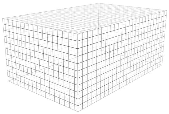
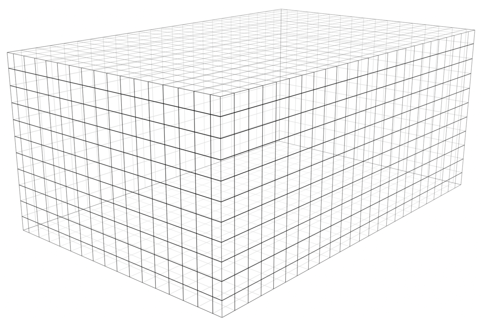
For visual orientation, Figure 1 shows the corresponding box geometry; the corresponding rendering is available on GitHub; see [10]. The illustration highlights the relative proportions of the side lengths and serves as a geometric reference for the numerical reconstruction discussed below.
Figure 1.
Rectangular box with , , and .
3.1. Generating the Eigenvalues
To generate a sufficiently large and accurate sample of Dirichlet eigenvalues for the rectangular box with side lengths , , and , we exploit the exact separability of the Laplacian in Cartesian coordinates. The Dirichlet eigenvalues are given explicitly by Equation (2). By enumerating all integer triples up to a large cutoff and sorting the resulting values in ascending order, we obtain a substantial portion of the low-lying Dirichlet spectrum. In the numerical experiments reported below, we retain the first few thousand. The corresponding Mathematica notebook is shown in Listing 1.
| Listing 1: Generation of Dirichlet eigenvalues for the box Ω(1, 1.5, 2.3). |
 |
The resulting set of eigenvalues is exported to a text file for subsequent processing. The notebook used to generate the spectrum is available on GitHub; see [11]. For reference, the first 15 and the last 5 eigenvalues of the 20,000 generated values are
| 16.121804, | 21.718934, | 29.281277, | 31.047482, | 34.878406, |
| 44.107450, | 44.206955, | 45.730618, | 51.213731, | 51.327747, |
| 56.810860, | 57.266923, | 58.890090, | 60.656295, | 60.898838, |
| … | ||||
| 5142.949068, | 5143.034062, | 5143.471467, | 5143.471467, | 5143.929602 |
3.2. Extracting the Weyl Coefficients
Starting from the numerically generated Dirichlet spectrum , the Weyl coefficients are extracted via the short-time asymptotics of the heat trace given by the sum (4). Rather than fitting the counting function directly, the heat trace approach provides improved numerical stability and allows for a clean separation of the different asymptotic contributions.
3.2.1. Choice of the Time Window
Since only a finite portion of the spectrum is available, the time interval must be chosen carefully. To suppress contributions from the truncated spectral tail, the window is scaled relative to the largest eigenvalue according to
with fixed dimensionless factors and . For the present example with eigenvalues, we use and , ensuring that is negligible throughout the fitting range. The heat trace is evaluated on a logarithmically spaced grid of 251 points within this interval.
3.2.2. Heat Trace Fit
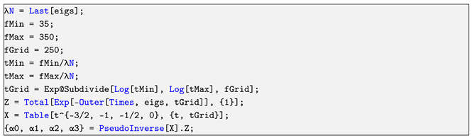
As introduced in Equations (4) and (5), the Weyl coefficients are recovered from the fitted heat trace coefficients . Numerically, the coefficients are obtained by a linear least-squares fit of the computed heat trace against the basis functions , , , and a constant term. This results in a small overdetermined linear system, which is solved using the pseudoinverse, as implemented in Listing 2.
| Listing 2: Heat trace evaluation and linear fit. |
 |
3.2.3. Conversion to Weyl Coefficients
The coefficients obtained from the heat trace fit are related to the Weyl coefficients through the standard correspondence between heat-kernel asymptotics and the spectral counting function. In the normalization adopted throughout this paper, the leading coefficient determines the volume term via Equation (7), while the coefficient yields the surface-area contribution according to Equation (8). The numerical extraction of the heat coefficients is performed by a linear least-squares fit of the truncated heat trace, as described above and implemented in Listing 2; their conversion into Weyl coefficients is carried out in Listing 3.
The third Weyl coefficient requires special care for the rectangular box since the boundary is not smooth and the classical geometric interpretation in terms of integrated mean curvature of a smooth boundary does not apply. Instead, the coefficient of the term is determined spectrally from the exact factorization of the Dirichlet heat trace. This yields the genuine Weyl coefficient , from which follows via Equation (9). The numerical extraction and conversion of this term are handled analogously and are included in Listings 2 and 3.
| Listing 3: Conversion from heat coefficients to Weyl coefficients. |
 |
3.2.4. Validation Against Exact Values
For the rectangular box, all Weyl coefficients are known in closed form. This allows for a direct and unambiguous validation of the spectral extraction procedure. In particular, the first and second coefficients correspond to the volume and surface area of the domain, while the third coefficient incorporates the non-smooth edge contribution characteristic of polyhedral boundaries.
Table 3 compares the Weyl coefficients and the associated geometric invariants obtained from the heat trace fit against their exact theoretical values. For all quantities considered, the relative deviation remains below , demonstrating excellent agreement. This confirms that the proposed heat-based extraction method recovers not only the leading volume and surface terms, but also the subtle third Weyl coefficient associated with edge effects, with high numerical accuracy.
Table 3.
Validation of spectrally extracted Weyl coefficients against exact values for the rectangular box.
3.3. Reconstructing the Sides
Once the Weyl coefficients , , and have been extracted from the spectrum, the reconstruction of the side lengths reduces to solving a single cubic equation. As shown in Section 2.3, the side lengths are given by the three positive real roots of the polynomial (10).
In practice, the roots of this equation are computed numerically. Since the rectangular box yields three strictly positive real solutions, the reconstructed side lengths are obtained by taking the real parts of the roots and sorting them in ascending order. The corresponding implementation in Mathematica is shown in Listing 4.
| Listing 4: Reconstruction procedure based on the Weyl coefficients. |
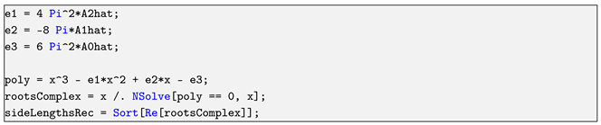 |
Table 4 summarizes the reconstructed side lengths obtained from the spectrally extracted Weyl coefficients and compares them to the exact geometric values. All three side lengths are recovered with relative errors below , confirming the accuracy and numerical stability of the reconstruction procedure.
Table 4.
Side lengths reconstructed via Listing 4.
4. Can Fewer Eigenvalues Suffice?
A natural practical question is how many Dirichlet eigenvalues are required in order to reliably extract the Weyl coefficients, in particular the third coefficient , which is known to be the most sensitive to truncation effects and numerical noise.
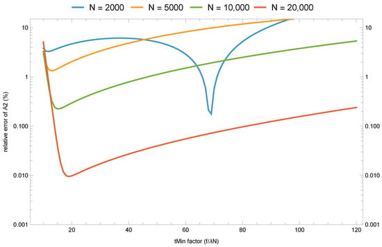
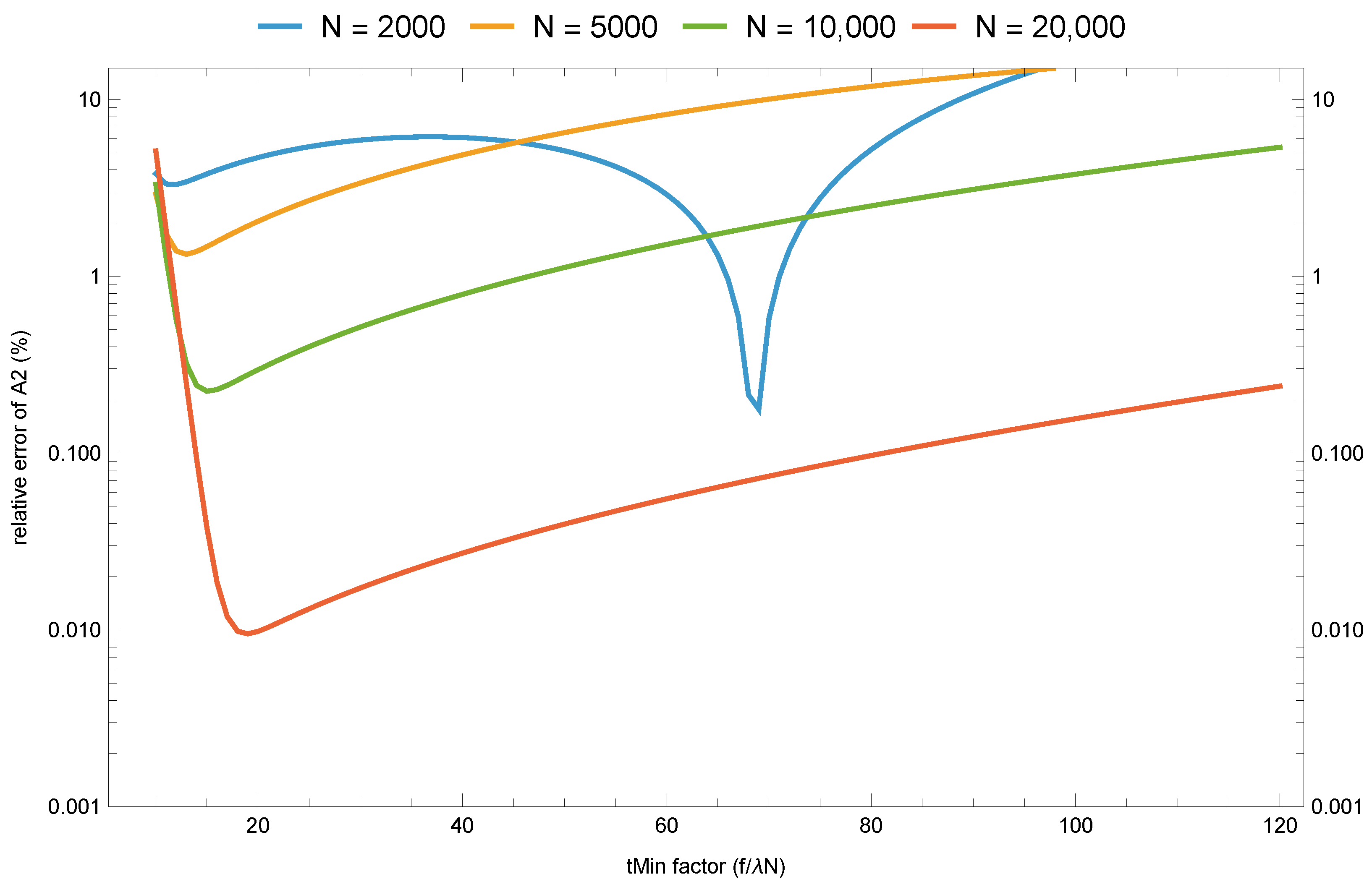
To address this question, we repeat the heat trace-based extraction procedure for progressively smaller subsets of the spectrum. Starting from the full set of 20,000 eigenvalues, we truncate the spectrum to 10,000, 5000, and 2000 eigenvalues, and study the relative error in the reconstructed coefficient as a function of the lower bound of the heat trace fitting window. In all cases, the upper bound is chosen sufficiently large to suppress higher-order terms of the heat expansion. For each truncation level N, the relative error in exhibits a pronounced stability minimum as is varied.
A robust empirical scaling is that the optimal lower bound scales with the inverse of the largest available eigenvalue,
where the dimensionless constant depends on the truncation level and, as we show later, on the box aspect ratios, as well as on the conditioning of the least-squares design matrix used in the heat trace fit. In the reduced spectrum with eigenvalues in our working example, we observe . This scaling law is clearly visible in Figure 2, which shows the relative error of as a function of the dimensionless parameter for different truncation levels. In particular, we find that already eigenvalues are sufficient to recover with relative errors below one percent, provided the fitting window is chosen according to Equation (11). This demonstrates that the proposed procedure does not require extremely large spectral data sets and that the third Weyl coefficient can be extracted robustly even from moderately sized spectra, as long as the time window is selected in a controlled manner.
Figure 2.
Relative error of the reconstructed Weyl coefficient as a function of the dimensionless parameter for different truncation levels N.
As shown in Figure 2, all curves exhibit a pronounced stability minimum, reflecting the balance between truncation errors at very small times and the influence of subleading heat terms at larger times. However, the location of the minimum is not universal across truncation levels: the optimal dimensionless cutoff depends noticeably on N for the present data set. In particular, in Figure 2 the minimizer shifts to smaller values of f as more eigenvalues are included, while for the most strongly truncated spectrum () the minimum occurs near .
Guided by Figure 2, we choose for the reduced experiment with eigenvalues since this value is near the observed stability minimum in that truncation regime. We keep and use a logarithmic grid with 251 sampling points. We then repeat the full extraction and reconstruction procedure using only the first Dirichlet eigenvalues.
Despite the substantial reduction of spectral input data, the reconstructed Weyl coefficients remain in very good agreement with their exact values. In particular, the third Weyl coefficient , which is most sensitive to truncation effects, is recovered with a relative error well below one percent. The resulting geometric quantities derived from the Weyl coefficients show comparable accuracy; see Table 5.
Table 5.
Reconstruction of Weyl coefficients and derived geometric quantities for the rectangular box using a reduced spectral input ( eigenvalues).
These results demonstrate that the proposed heat trace-based extraction of Weyl coefficients remains robust even when only a few thousand eigenvalues are available. In particular, once the stability minimum of the heat-time window is respected, no fine-tuning of parameters is required. This makes the method well-suited for applications in which the numerical computation of very high eigenvalues is prohibitively expensive, such as curved or non-separable geometries.
4.1. A Stability Landscape Across Box Aspect Ratios
So far an empirical scaling rule has been established for the working example . We now probe how universal this constant is by repeating the stability-minimum search across a wide family of rectangular boxes.
The Dirichlet spectrum of a box is invariant under uniform scaling in the sense that . Hence, it suffices to fix and to parameterize shapes by the aspect ratios
We sample on a logarithmic grid in the range . For each shape , we generate the first exact eigenvalues from (2).
Let us approach a definition of the stability minimum . For a fixed spectrum truncation N, we evaluate the truncated heat trace on a logarithmic time grid over with
and we perform a four-term heat trace fit by linear least squares. From the fitted coefficient we obtain the spectral estimate
which can then be compared to the exact expression (9). For the Dirichlet box, the third Weyl coefficient is known as ; see Equation (9). We therefore scan and define the stability minimum as
From a numerical perspective, the heat trace fit underlying the definition of can be viewed as a linear regression problem. For each choice of , the sampled heat trace values are assembled into a data vector, while the corresponding design (feature) matrix is given by
where denotes the logarithmically spaced time grid. The heat coefficients are then obtained by solving the overdetermined linear system in the least-squares sense. The stability minimum thus identifies the regime in which this regression problem is optimally conditioned with respect to the extraction of the coefficient , and hence of the Weyl coefficient .
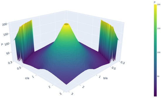
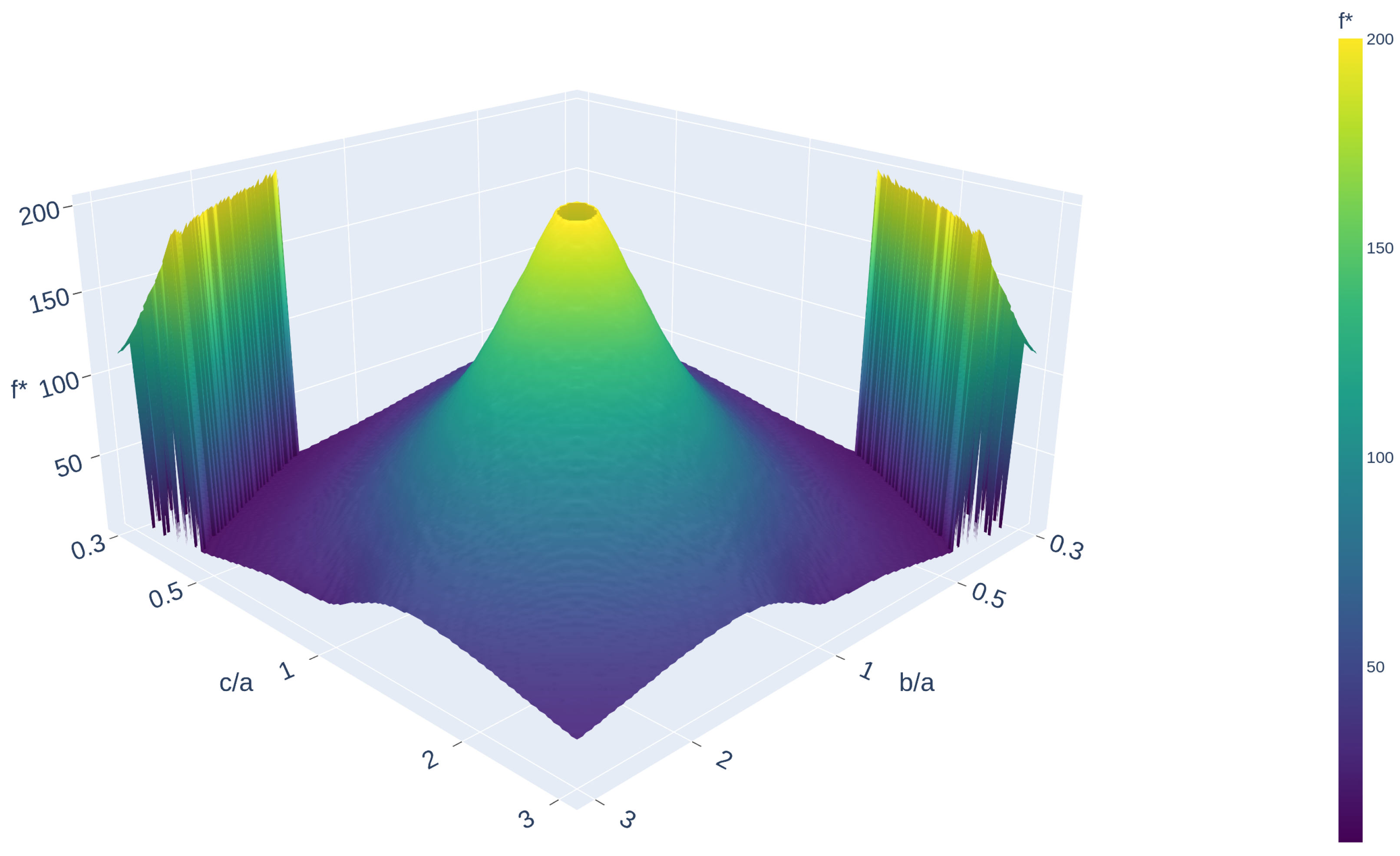
Figure 3 visualizes the map as a 3D surface in the aspect-ratio variables , with logarithmic scaling applied to both horizontal axes, generated with the notebook [12]. Rather than a single universal constant, depends strongly on the aspect ratios. Moderately anisotropic boxes cluster around to 80, including the working example with . Near the isotropic cube regime , forming a shallow basin in the stability landscape, the optimum drops markedly to . For highly anisotropic boxes (one side much smaller than the other), decreases again and can reach values close to the lower end of our scan. By symmetry, the landscape is invariant under swapping x and y and overall exhibits a pronounced ridge-and-crater structure reminiscent of a “volcano”.
Figure 3.
Stability landscape for the Dirichlet box with .
Here, denotes the dimensionless heat-time cutoff that minimizes the relative error of the reconstructed third Weyl coefficient in a four-term heat trace fit based on eigenvalues.
The stability-minimum search remains robust and inexpensive (it requires only a one-dimensional scan in f once the spectrum is available), and it provides an automatic, geometry-adaptive choice of for truncated spectral data.
4.2. Stability Minimum from Optimal Truncation in Laplace-Type Asymptotics
We now move from the empirical observation of the stability minimum to a heuristic asymptotic explanation based on Laplace-type analysis. In particular, the onset of the stability minimum (visible as a “crimp” in Figure 2) marks the regime in which exponentially suppressed truncation errors and algebraically growing model errors become comparable.
The following analysis is intended as a heuristic asymptotic explanation of the observed stability minimum. It relies on replacing the discrete spectral measure by its Weyl asymptotic density, which introduces an uncontrolled approximation error. Accordingly, the derivation does not constitute a rigorous proof but rather provides a consistent asymptotic interpretation of the numerical observations. The resulting relations should therefore be understood as heuristic principles, supported by both classical asymptotic theory and the empirical stability behavior observed in the numerical experiments.
To formalize this intuition, we recall a classical result from Laplace-type asymptotics. Bender and Orszag analyze integrals of the form as , see [13] (p. 261). On p. 267 they derive the leading asymptotic contribution in the case when has a nondegenerate interior maximum at , so that and . For this yields
Defining the x-independent prefactor K, we obtain the structural form , that is, an exponential factor multiplied by the algebraic prefactor with an x-independent constant K. In our cutoff problem the relevant contribution is exponentially suppressed. We therefore rewrite the exponent in (12) in decay form by setting with , so that . This yields .
For the balance argument, only the exponential–algebraic structure matters; the x-independent constant K and the precise value of are not essential. We therefore reduce the expression to the structural template as , with an algebraic exponent determined by the specific setting (for Laplace’s method in the nondegenerate case, ). Note that although the heat trace itself is analyzed in the short-time regime , the relevant asymptotic parameter in the truncated tail is the dimensionless quantity . In the stability-minimum regime one has , so f plays precisely the role of the large parameter x in Laplace’s method.
To connect this structural template with our spectral problem, we begin with the exact identity
where denotes the eigenvalue counting function. The only approximation step in the subsequent reasoning consists in replacing the discrete spectral measure by its Weyl asymptotic density in three dimensions, with denoting the density constant resulting from differentiating the leading term of the counting function . While this replacement is standard in spectral asymptotics, we do not provide explicit error bounds here. Accordingly, all subsequent relations should be interpreted in a heuristic asymptotic sense. This replacement yields a continuous Laplace-type integral whose tail can be analyzed using standard asymptotic methods. Thus, the Laplace analogy enters precisely at the level of the Weyl approximation and does not affect the discrete fitting procedure itself. This approximation is expected to be accurate in the high-frequency regime , but we do not quantify the associated remainder term.
Using Weyl’s law in three dimensions (Appendix C), the truncated spectral tail admits the representation . We provide an explicit representation of the truncated spectral tail in terms of incomplete Gamma functions, which enables a direct asymptotic analysis of the reconstruction error. Hence the tail inherits the same “exponential times power” structure and for large f, , which is precisely of the form (with and ).
A central message here is the principle of optimal truncation: asymptotic approximations are most accurate when truncated near the point where the exponentially small remainder becomes comparable (in its effect) to algebraic contributions; beyond that point, the remainder grows again. In our problem, the finite-eigenvalue approximation introduces a truncated spectral tail whose asymptotic behavior was derived above. For large f, the dominant contribution is of the form , i.e., it has the Laplace-type “exponential times power” structure. Since our regression model uses only finitely many heat terms, the first neglected contribution scales algebraically like .
According to the optimal truncation principle, the stability minimum occurs when the exponentially suppressed tail contribution and the algebraic model contribution have a comparable influence on the regression. Balancing the dominant contributions yields
and hence . Taking logarithms,
which yields the implicit relation
In our experiment, and . For , , yielding a combined logarithmic contribution of approximately .
The constant in (13) corresponds to an effective prefactor in the relation , so that the constant term equals . For our numerical values (, ), this yields , and hence . The prefactor collects geometric constants as well as the sensitivity of the least-squares regression.
The stability minimum reflects optimal truncation in Laplace-type asymptotics, where exponentially suppressed spectral-tail effects balance algebraically growing model errors.
We emphasize that the following statements are not intended as fully rigorous theorems. The derivations rely on replacing the discrete spectral measure by its Weyl asymptotic density, which introduces an uncontrolled approximation error. Accordingly, the following results should be interpreted as heuristic asymptotic principles, supported by numerical evidence, rather than strict mathematical propositions.
Heuristic Statement 1
(Stability minimum). Under Weyl asymptotics and truncated heat trace fitting, the optimal lower cutoff satisfies asymptotically the implicit relation (13), i.e., . This reflects the balance between exponentially suppressed truncation errors and algebraic model errors, in accordance with the principle of optimal truncation in Laplace-type asymptotics.
This relation reflects the competition between exponential suppression and algebraic contributions: the exponential term induces linear dependence in f, while algebraic terms contribute only logarithmically.
While the asymptotic relation (13) explains the existence of a stability minimum, it does not determine its location uniquely. We now make this dependence explicit in the following Heuristic Statement (2).
Heuristic Statement 2
(Dependence of the stability minimum). The stability minimum is not universal. Rather, it depends on three interacting components:
- 1.
- the spectral truncation level through N (equivalently through ),
- 2.
- the geometry of the domain through the box aspect ratios,
- 3.
- the conditioning of the least-squares design matrix used in the heat trace fit.
In particular, the stability minimum can be expressed as a derived quantity of the form
where denotes the conditioning of the regression matrix.
As indicated by Heuristic Statement 2, the conditioning of the regression matrix X plays a crucial role in determining the stability minimum. Regions of strong anisotropy exhibit pronounced oscillations in the estimated stability minimum, which we attribute to ill-conditioning of the regression matrix. These oscillations are clearly visible in Figure 3 and indicate a breakdown of the regression-based coefficient extraction in these regimes.
In contrast, the central region of the landscape forms a stability basin, where the minimum is well-defined and stable. This basin–ridge structure motivates a more systematic description of the stability landscape, which we formalize with Heuristic Statement (3), , the center of the stability basin, and , a deformation parameter.
- Define the deformed quadratic quantity
Heuristic Statement 3
(Empirical model of the stability landscape). In logarithmic coordinates , the stability landscape can be approximated as a rational function of the deformed quadratic quantity defined in (14), namely
where the parameters determine the geometry of the egg-shaped level sets, represents the baseline stability, and C scales the maximum amplitude of the stability peak.
To demonstrate that the level sets of the fitted stability landscape strictly follow the geometry defined by , we consider a contour of constant stability . By rearranging this expression, it is evident that the stability value depends solely on the value of the quadratic quantity . Consequently, any level set of the surface corresponds to a condition where The parameter introduces a u-dependent scaling of the -axis, which breaks the elliptical symmetry and generates the characteristic egg-shaped contours observed in the numerical data. While the rational profile determines the vertical decay and peak sharpness, the horizontal geometry is governed entirely by the isolines of .
The application of the rational model to the stability data demonstrates agreement, yielding a coefficient of determination . The low error metrics, with a root mean square error and a mean absolute error , confirm that the model accurately captures the global topology of the landscape. The parameter introduces a u-dependent scaling of the -axis, which breaks the elliptical symmetry and generates the characteristic egg-shaped contours observed in the numerical data. The optimized parameters for this stable configuration are summarized in Table 6.
Table 6.
Fitted parameters for the rational stability landscape.
4.3. Analytic Structure of the Baseline Contour
To better understand when the one-parameter rule of thumb is reliable, we consider the iso-contour
in the stability landscape shown in Figure 3. Here and denote the aspect ratios of the box with . Empirically, forms a closed curve surrounding the near-cube regime. It separates geometries for which the constant baseline performs well from regimes in which a geometry-adaptive choice of becomes preferable. In logarithmic aspect-ratio coordinates
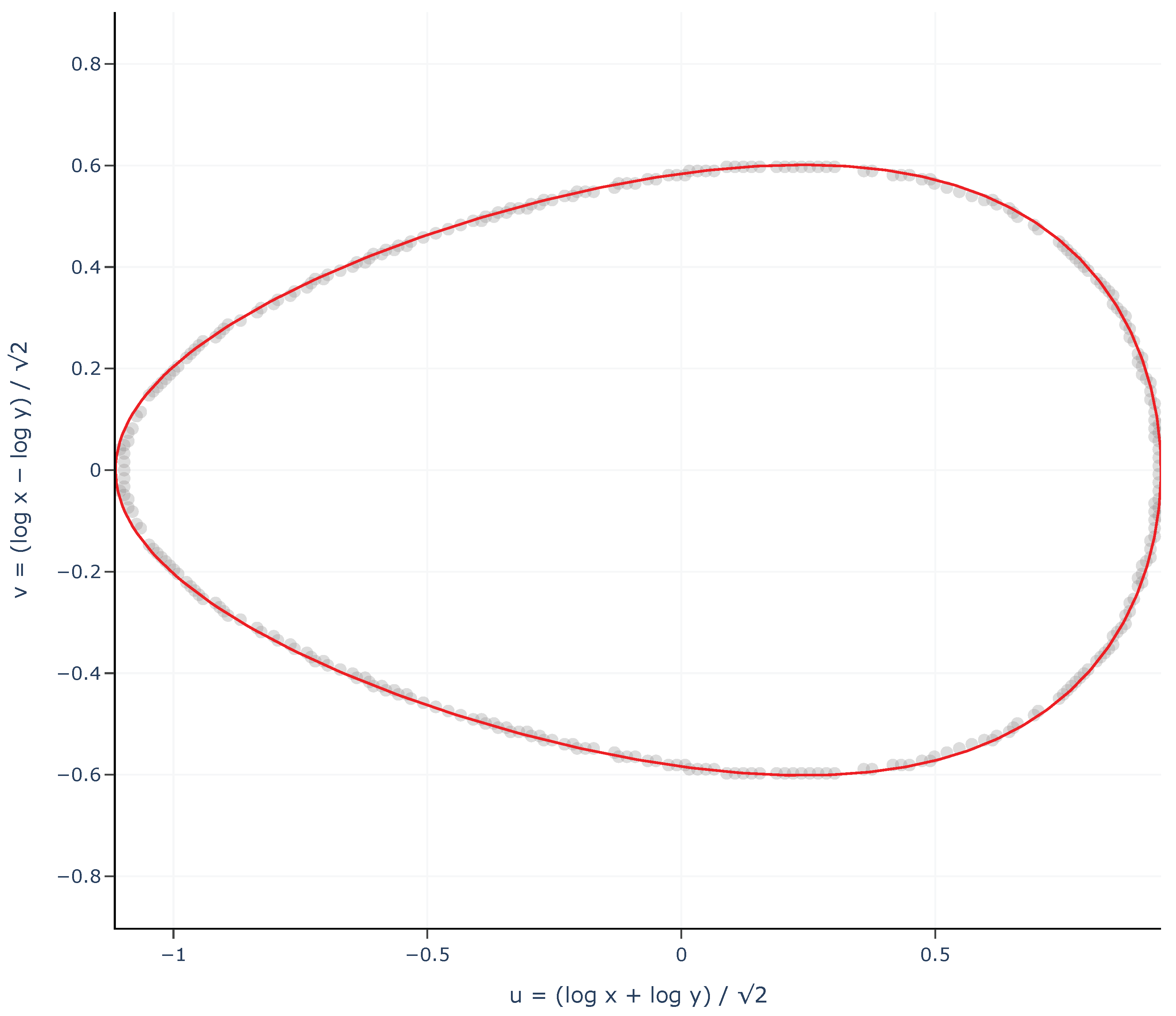
the contour exhibits a structured but slightly asymmetric shape. While a simple ellipse gives a rough approximation, the stability contour is more accurately captured by the implicit relation (17), defining the region where the constant cutoff is near-optimal for recovering . As shown in Appendix B, the stability boundary is defined by the level-set condition . Substituting the definition of the deformed quadratic quantity from (14), we obtain a rational algebraic plane curve of degree four that is birationally equivalent to a conic:
where the fitted parameters are , , and . In the limit , Equation (17) reduces to an ordinary ellipse. The additional factor in the denominator introduces a controlled deformation along the diagonal direction u, producing the empirically observed slightly egg-shaped contour. The model respects the symmetry under exchange , corresponding to , while allowing for anisotropic skewness along the u-direction. Numerically, the approximation achieves a root-mean-square deviation of approximately with respect to the extracted plateau, indicating that the contour is not merely elliptic but exhibits a reproducible and structured deformation.
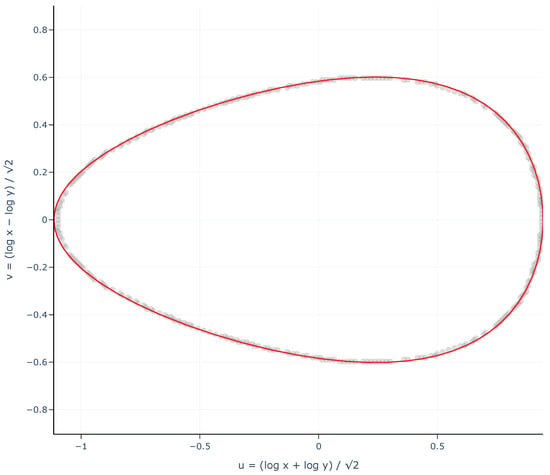
Figure 4 shows the extracted plateau in -coordinates together with the fitted egg-shaped contour (17) as computed by the notebook [14].
Figure 4.
Stability plateau in -coordinates together with the fitted implicit contour (17).
5. Outlook and Further Research
The reconstruction methodology presented in this work is deliberately validated on rectangular boxes, where exact spectral data and explicit Weyl coefficients are available. This provides a controlled setting in which the accuracy and stability of the approach can be assessed without additional numerical uncertainty. Importantly, the methodology itself does not rely on spectral separability, but only on the availability of sufficiently accurate eigenvalues. In particular, the heat trace-based extraction of Weyl coefficients and the stability-minimum phenomenon are expected to persist for general domains as they are governed by the universal short-time asymptotics of the heat kernel. A natural next step is therefore the extension to smooth curved geometries, such as ellipsoids or more general convex bodies, for which no closed-form eigenvalue expressions exist. In such cases, the third Weyl coefficient regains its classical geometric interpretation in terms of the integrated mean curvature of the boundary, providing direct access to curvature-related shape information. Extending the present framework to these geometries requires high-accuracy numerical eigenvalue computations on curved domains. While this introduces additional computational complexity, it does not entail conceptual changes to the reconstruction pipeline.
Another natural direction for further research concerns the a-priori determination of the optimal fitting window for truncated heat trace data. In the present work, the lower bound is chosen empirically by identifying a stability minimum in the reconstructed coefficient , which consistently occurs at the dimensionless value for the rectangular box. This behavior suggests that the optimal choice of is governed by a dimensionless balance between truncation effects due to the finite number of eigenvalues and deviations from the short-time heat trace asymptotics at larger times. A systematic modeling of this trade-off may lead to a predictive and fully automatic criterion for selecting the fitting interval, thereby avoiding visual inspection or prior calibration. Such an approach promises improved robustness and may generalize naturally to other geometries, higher dimensions, and different spectral truncation regimes.
A natural extension concerns other boundary conditions. For Neumann boundary conditions, the leading Weyl term remains unchanged, while boundary contributions enter with different signs in the heat trace expansion. In particular, the interpretation of subleading coefficients differs, reflecting the altered spectral boundary behavior. For mixed (Robin) boundary conditions, additional terms depending on the boundary operator appear, which complicate the extraction of geometric information. Extending the present framework to such settings requires a careful analysis of how boundary conditions affect the identifiability of Weyl coefficients.
Another important direction concerns robustness with respect to noisy spectral data. In practical scenarios, eigenvalues are subject to measurement errors or numerical approximations. While the present results are based on exact spectral input, the stability analysis suggests that the reconstruction procedure depends on a balance between truncation effects and model sensitivity. A systematic study of how perturbations in the eigenvalues propagate through the heat trace fitting and affect the recovered Weyl coefficients remains an important topic for future work. This suggests that the stability minimum may also play a role in mitigating noise amplification, a hypothesis that warrants further investigation. Such investigations may benefit from regularization strategies or robust regression techniques, particularly in regimes near the stability minimum.
Author Contributions
Conceptualization, E.S.; Methodology, E.S.; Software, E.S., C.M. and A.H.; Validation, A.H. and E.S.; Formal Analysis, E.S. and A.H.; Investigation, E.S., C.M. and A.H.; Resources, E.S.; Data Curation, C.M., A.H. and E.S.; Writing—Original Draft Preparation, E.S., A.H. and C.M.; Writing—Review and Editing, E.S. and N.K.; Visualization, E.S., A.H. and C.M.; Supervision, E.S. and N.K.; Project Administration, E.S. All authors have read and agreed to the published version of the manuscript.
Funding
This research received no external funding.
Institutional Review Board Statement
Not applicable.
Data Availability Statement
The original contributions presented in this study are included in the article. Further inquiries can be directed to the corresponding author.
Acknowledgments
I am grateful to Elmar Schrohe for suggesting the study of inverse spectral questions, for inspiring the investigation of how geometric information can be recovered from eigenvalue data, and for his valuable support.
Conflicts of Interest
Author Cornelius May was employed by the company Capgemini Deutschland GmbH. The remaining authors declare that the research was conducted in the absence of any commercial or financial relationships that could be construed as a potential conflict of interest.
Appendix A. Derivation of the Third Weyl Coefficient for the Dirichlet Box
We derive the explicit expression for the third Weyl coefficient of a rectangular box with Dirichlet boundary conditions. The derivation relies on the exact factorization of the heat trace into one-dimensional contributions and makes explicit the origin of the additional term arising from the non-smooth boundary of the box. We follow the general definition of the heat trace introduced in Section 2.2. For the Dirichlet Laplacian on an interval , we denote the associated heat trace by .
Since the spectrum of the one-dimensional Dirichlet Laplacian on an interval of length a is explicitly given by , , see [15] (p. 322) and [16] (p. 283), the heat trace can be written as
In the presence of a boundary, we need to use the asymptotic expansion (6). Restricting the inner sum to its first two algebraic terms, corresponding to and , yields the one-dimensional Dirichlet contribution and hence after inserting and . Here, the limit is understood, while the remaining contributions are exponentially suppressed. The leading coefficient equals the volume of M, whereas the terms with half-integer powers arise from boundary contributions. As shown in [5] (p. 192), for Dirichlet boundary conditions, one has
In this context denotes the 0-dimensional Hausdorff measure. For the boundary consists of two points, , and thus . In our one-dimensional setting , we have , , and . Inserting these values into (A2) yields . Substituting this coefficient into the prefactor of Equation (6) then gives
which is precisely the short-time asymptotic expansion used in the subsequent factorization argument. The constant term reflects the presence of the Dirichlet boundary. For the rectangular box , separation of variables and the explicit one-dimensional heat trace (A1), which legitimizes the product structure, imply an exact factorization of the heat trace, , where and are defined analogously. Writing with (and similarly , ), we obtain
Expanding this product yields
Consequently, the coefficient of the term is given by
Appendix B. Conic Reduction of Stability Boundaries
For clarity, we outline the key steps of the transformation before presenting the algebraic derivation. We start from the implicit stability relation (17). For notational simplicity, we introduce the shifted coordinate and set . Equation (17) then takes the form
Rational plane curves admit representations of the form (A5), where , and are polynomials sharing a common denominator (cf. Piegl & Tiller [17] (p. 26)).
In the present case, the nonlinear deformation of the ellipse is entirely induced by the rational factor in the x-coordinate. This suggests introducing the rational change of variable
Substituting into (A4) eliminates the rational deformation and yields , an ellipse.
Since both maps are rational inverses of each other, the two curves are birationally equivalent. There is only one conic in a projective plane, i.e., all nondegenerate (smooth) projective conics are projectively equivalent [18] (p. 252). Such a conic is rational and birational to the projective line [19] (p. 73). Since has genus 0 [20] (p. 548) and birational transformation conserves the genus [21] (p. 544), [22] (p. 179), any smooth conic and thus the stability boundary is likewise a genus-zero curve. Clearing denominators in the Equation (A4) yields a quartic, that is, a polynomial equation in of total degree four. As the coordinate change (A6) is a birational self-map of the projective plane, it lies in the Cremona group (cf. [23] (p. 29)), so the quartic stability boundary arises from a conic via a Cremona transformation.
Appendix C. Derivation of the Γ(, f)-Structure from Weyl’s Law
We briefly justify the appearance of the exponent in the incomplete Gamma function governing the truncated spectral tail. In dimension , Weyl’s law implies that the spectral density satisfies as for some geometry-dependent constant C. Replacing the discrete spectral tail by its integral approximation, we obtain
With the change of variables , and , the integral becomes
The remaining integral is precisely the upper incomplete Gamma function, . Hence . In general dimension d, Weyl’s law gives , leading to , so the exponent is the special case .
References
- Pinchover, Y.; Rubinstein, J. An Introduction to Partial Differential Equations; Cambridge University Press: Cambridge, UK, 2005. [Google Scholar] [CrossRef] [Scilit]
- Brack, M.; Bhaduri, R.K. Semiclassical Physics; Addison-Wesley: Boston, MA, USA, 1997. [Google Scholar]
- Safarov, Y.; Vassiliev, D. The Asymptotic Distribution of Eigenvalues of Partial Differential Operators; American Mathematical Society: Providence, RI, USA, 1997. [Google Scholar]
- Ivrii, V.Y. Second term of the spectral asymptotic expansion of the Laplace-Beltrami operator on manifolds with boundary. Funct. Anal. Its Appl. 1980, 14, 98–106. [Google Scholar] [CrossRef] [Scilit]
- Levitin, M.; Mangoubi, D.; Polterovich, I. Topics in Spectral Geometry; American Mathematical Society: Providence, RI, USA, 2023. [Google Scholar]
- Gowers, T.; Barrow-Green, J.; Leader, I. (Eds.) The Princeton Companion to Mathematics; Princeton University Press: Princeton, NJ, USA; Oxford, UK, 2008. [Google Scholar]
- Gottlieb, H.P.W. Eigenvalues of the Laplacian for rectilinear regions. ANZIAM J. 1988, 29, 270–281. [Google Scholar] [CrossRef] [Scilit]
- McKean, H.P.; Singer, I.M. Curvature and the eigenvalues of the Laplacian. J. Differ. Geom. 1967, 1, 43–69. [Google Scholar] [CrossRef] [Scilit]
- Manfrino, R.B.; Ortega, J.A.G.; Delgado, R.V. Topics in Algebra and Analysis: Preparing for the Mathematical Olympiad; Birkhäuser: Basel, Switzerland, 2015. [Google Scholar] [CrossRef] [Scilit]
- Sultanow, E. 3D Rendering of the Rectangular Box Geometry. Blender Rendering File, Cone-Operator-Lab Repository. 2026. Available online: https://github.com/Sultanow/cone-operator-lab/blob/main/renderings/box_a1.0_b1.5_c2.3.blend (accessed on 3 April 2026).
- Sultanow, E. Numerical Generation of Dirichlet Laplacian Eigenvalues on a Rectangular Box. Mathematica Notebook, Cone-Operator-Lab Repository. 2026. Available online: https://github.com/Sultanow/cone-operator-lab/blob/main/mathematica/Hearing_Box_GenerateEigenvalues.nb (accessed on 3 April 2026).
- Sultanow, E. Stability Landscape Analysis and Volcano Surface Visualization (3D). Mathematica Notebook, Cone-Operator-Lab Repository. 2026. Available online: https://github.com/Sultanow/cone-operator-lab/blob/main/mathematica/Hearing_Box_AnalyzeStabilit%C3%A4tsminimum.nb (accessed on 3 April 2026).
- Bender, C.M.; Orszag, S.A. Advanced Mathematical Methods for Scientists and Engineers I: Asymptotic Methods and Perturbation Theory; Springer: Berlin/Heidelberg, Germany, 1999. [Google Scholar]
- Sultanow, E. Stability Plateau Extraction and Egg-Contour Fitting (2D). Jupyter Notebook, Cone-Operator-Lab Repository. 2026. Available online: https://github.com/Sultanow/cone-operator-lab/blob/main/python/notebooks/Hearing_Box_ReconstructWeylCoeffs_HeatEquation_CalcStabilit%C3%A4tsminimumA2-2D.ipynb (accessed on 3 April 2026).
- Strauss, W.A. Partial Differential Equations: An Introduction, 2nd ed.; John Wiley & Sons: Hoboken, NJ, USA, 2008. [Google Scholar]
- O’Neil, P.V. Beginning Partial Differential Equations, 2nd ed.; John Wiley & Sons: Hoboken, NJ, USA, 2008. [Google Scholar]
- Piegl, L.; Tiller, W. The NURBS Book, 2nd ed.; Springer: Berlin/Heidelberg, Germany, 1997. [Google Scholar]
- Glaeser, G.; Stachel, H.; Odehnal, B. The Universe of Conics, 2nd ed.; Springer: Berlin/Heidelberg, Germany, 2024. [Google Scholar] [CrossRef] [Scilit]
- Shafarevich, I.R. Basic Algebraic Geometry 1: Varieties in Projective Space, 3rd ed.; Springer: Berlin/Heidelberg, Germany, 2013. [Google Scholar] [CrossRef] [Scilit]
- Görtz, U.; Wedhorn, T. Algebraic Geometry II: Cohomology of Schemes; Springer: Berlin/Heidelberg, Germany, 2023. [Google Scholar] [CrossRef] [Scilit]
- Forsyth, A.R. Theory of Functions of a Complex Variable, 3rd ed.; Dover: New York, NY, USA, 1965; Volume 2. [Google Scholar]
- Walker, R.J. Algebraic Curves; Springer: Berlin/Heidelberg, Germany, 1978. [Google Scholar]
- Alberich-Carramiñana, M. Geometry of the Plane Cremona Maps; Springer: Berlin/Heidelberg, Germany, 2002. [Google Scholar] [CrossRef] [Scilit]

Disclaimer/Publisher’s Note: The statements, opinions and data contained in all publications are solely those of the individual author(s) and contributor(s) and not of MDPI and/or the editor(s). MDPI and/or the editor(s) disclaim responsibility for any injury to people or property resulting from any ideas, methods, instructions or products referred to in the content. |
© 2026 by the authors. Licensee MDPI, Basel, Switzerland. This article is an open access article distributed under the terms and conditions of the Creative Commons Attribution (CC BY) license.