On Contraction Principles in Product Spaces and Applications in Iterated Function Systems

Abstract

This paper develops an extension of the research work by Proinov to the product spaces $X^{\left|I\right|}$ (I is representing an indexing set). This paper also introduces a novel class of $(\mathcal{L};\mathcal{Y})$-contractions defined on a supremum metric $(X^{\left|I\right|},d^{\prime })$. In supremum metric $(X^{\left|I\right|},d^{\prime })$, several new fixed point theorems for $(\mathcal{L};\mathcal{Y})$-contractions have been established that generalize well-known ideas like the Banach, Geraghty, Boyd–Wong, and Wardowski principles. This paper also contributes a new iterated function system (IFS) built on the family of $(\mathcal{L};\mathcal{Y})$-contractions and demonstrates the existence and uniqueness of fractals (in other words, compact attractors) in a complete supremum metric $(X^{\left|I\right|},d^{\prime })$. Theoretical work is illustrated with examples and graphs.

1. Introduction and Preliminaries

Fixed point theory (FPT) is a dynamic and fascinating area of mathematics, combining elements of geometry, topology, and analysis. Over the last few decades, fixed points have become a central tool for studying nonlinear systems. In 1922, the Polish mathematician Stefan Banach [1] proved a fundamental theorem on the existence and uniqueness of fixed points for contraction mappings in complete metric spaces (CMS), marking a milestone in metric fixed point theory.

Boyd and Wong [2] (1969) generalized Banach’s contraction principle by replacing the contraction constant with a function, improving earlier results by Browder [3] (1968) and Rakotch [4] (1962). The concept of $(\mathcal{L};\mathcal{M})$-contractions [5] further extends classical mappings by incorporating two auxiliary functions, $\mathcal{L}$ and $\mathcal{M}$, allowing more flexible conditions in metric spaces, especially in noncontinuous or partially ordered settings. Proinov formalized a class of generalized contractive mappings

$$\mathcal{L}\left(d\right(Tx,Ty\left)\right)\le \mathcal{M}\left(d\right(x,y\left)\right),$$

where T is a self-mapping on $(X,d)$, and $\mathcal{L}$ and $\mathcal{M}$ are monotone functions satisfying additional conditions, providing a broader framework for fixed point theorems.

Building on Proinov, Chanda et al. (2021) [6] introduced $(\mathcal{L};\mathcal{M})$-Wardowski contraction pairs, which do not require continuity at fixed points—a significant departure from classical theorems. They proved a common fixed point theorem in complete metric spaces and demonstrated applications to fractional differential equations, functional equations in dynamic programming, and nonlinear quadratic integral equations, illustrating the framework’s versatility across physics, economics, and engineering.

Further developments include $(\mathcal{L};\mathcal{M})$-type Suzuki contractions [7], contractive iterates [8], and $(\alpha ,\beta ,\mathcal{L},\mathcal{M})$-interpolative contractions [8], which unify various fixed point principles and establish sufficient and necessary conditions for existence and uniqueness. Wasey et al. (2025) [9] refined Proinov-type relational contractions using locally transitive relations and test functions $(\mathcal{L};\mathcal{M})$, applying them to boundary value problems.

In the context of set-valued mappings, Markin was the first to use the Pompeiu–Hausdorff (PH) metric to study fixed points for set-valued mappings. In 1969, Nadler [10] established a multivalued version of Banach’s fixed point theorem. Since then, many mathematicians have defined various contractions and multivalued contraction-type mappings (see, e.g., [11,12,13,14]).

Inspired by multivalued contractions, Barnsley [15] and Hutchinson [16] introduced the concept of iterated function systems (IFSs) consisting of families of contractions (see also [17]). Subsequently, many authors [18,19,20,21,22,23,24,25,26] studied finite IFSs built from different contractions [27]. From the literature on fractal theory, the authors in [28] noted that finite IFSs composed of generalized contractive mappings can be effectively studied only when the mappings satisfy a commutativity assumption. Recently, Secelean [29,30] extended fractal theory to countable IFSs. Continuing this work, Hata [31] and Wicks [32] developed the concept of infinite IFSs (see also [33]).

Building on these contributions, Secelean [34] introduced IFSs based on families of F-contractions and studied the existence and uniqueness of fractals. Gwózdz-Lukawska and Jachymski [35] studied finite IFSs on metric spaces equipped with directed graphs. Pasupathi et al. [36] examined a novel IFS related to generalized $\theta$-contractions. Dumitru [37] studied generalized IFSs built on Meir–Keeler-type mappings (see also Strobin and Swaczyna [38]).

The theoretical framework of fixed point theory and fractal construction is further strengthened by recent developments. Cui et al. (2025) [39] studied expansive measures in nonautonomous IFS, providing a modern measure-theoretic characterization of dynamical behavior, while Thangaraj et al. (2024) [40] constructed fractal attractors via Kannan contractions in controlled metric spaces. These works highlight that contraction principles should describe not only existence but also structural and geometric properties of attractors.

Motivated by these advances, this article extends the $(\mathcal{L};\mathcal{M})$-contraction framework to product spaces $X^{\left|I\right|}$ with the supremum metric, proving new fixed point theorems that generalize Banach, Boyd–Wong, Geraghty, and Wardowski results. Iterated function systems composed of $(\mathcal{L};\mathcal{M})$-contractions are defined, and the existence and uniqueness of fractals in complete metric spaces are established, along with convergence of iterative sequences. Examples, lemmas, and theorems are presented for $(\mathcal{L};\mathcal{M})$-contractions in product spaces, and a method for fractal generation with geometric representation is developed.

2. Preliminary Results

This section summarizes the essential preliminaries, including the metric structure of product spaces and the $(\mathcal{L};\mathcal{Y})$-contractive conditions that underpin our main results.

Lemma 1 

([5]). Assume that $(X,d)$ is a metric space and that $\left\{x_n\right\}$ is a non-Cauchy sequence in X. and ${lim}_{n\to \infty }d(x_n,x_{n+1})=0$. Then there is some $\epsilon >0$ and two sub-sequences $\left\{x_{n_k}\right\}$ and $\left\{x_{m_k}\right\}$ of the sequence $\left\{x_n\right\}$ so that

$$\underset{k\to \infty }{lim}d(x_{n_{k+1}},x_{m_{k+1}})={\epsilon }^{+}.$$

(1)

$$\underset{k\to \infty }{lim}d(x_{n_k},x_{m_k})=\underset{k\to \infty }{lim}d(x_{n_k},x_{m_{k+1}})=\underset{k\to \infty }{lim}d(x_{n_{k+1}},x_{m_k})=\epsilon .$$

(2)

Lemma 2 

([5]). For a function $\mathcal{L}:(0,\infty )\to \mathbb{R}$ the conditions stated below are equivalent:

(a)

$\underset{t>\epsilon }{inf}\mathcal{L}\left(t\right)>-\infty$ for any positive ε.

(b)

$\underset{t\to {\epsilon }^{+}}{lim\; inf}\mathcal{L}\left(t\right)>-\infty$ for any positive ε.

(c)

$\underset{n\to \infty }{lim}\mathcal{L}\left(t_n\right)=-\infty$ implies that $\underset{n\to \infty }{lim}{t}_n=0$.

Lemma 3 

([5]). For a function $\mathcal{M}:(0,\infty )\to \mathbb{R}$ with $\underset{n\to \infty }{lim}\mathcal{M}\left(t_n\right)=0\Rightarrow \underset{n\to \infty }{lim}{t}_n=0$, the following inequality always hold

$$\underset{t\to \epsilon }{lim}(inf\mathcal{M}\left(t\right))>0\mathit{for}\mathit{any}\mathit{positive}\epsilon >0.$$

Lemma 4 

([5]). The conditions stated below are equivalent for the function $\mathcal{Y}:(0,\infty )\to (0,\infty )$.

(a)

If $\underset{n\to \infty }{lim}{t}_n=\epsilon >0$, then $\underset{n\to \infty }{lim}inf\mathcal{Y}\left(t_n\right)>0$.

(b)

A sequence $\left\{t_n\right\}$ which is bounded if $\underset{n\to \infty }{lim}\mathcal{Y}\left(t_n\right)=0$, then $\underset{n\to \infty }{lim}{t}_n=0$.

(c)

$\underset{t\to \epsilon }{lim}inf\mathcal{Y}\left(t\right)>0$, where ε is any positive.

Lemma 5 

([5]). Let $\mathcal{L},\mathcal{Y}:(0,\infty )\to \mathbb{R}$ be two functions, then for a positive ε, the inequality given below holds true.

$$\underset{t\to \epsilon }{lim}sup\mathcal{Y}\left(t\right)<\underset{t\to \epsilon }{lim}inf\mathcal{L}\left(t\right).$$

(3)

Moreover, for a bounded sequence $\left\{t_n\right\}$, if both sequences $\left\{\mathcal{L}\left(t_n\right)\right\}$ and $\left\{\mathcal{Y}\left(t_n\right)\right\}$ converge to the same point, then $t_n\to 0$ as $n\to \infty$.

The above Lemma can equivalently be stated as follows:

Lemma 6 

([5]). Let $\mathcal{L}$ and $\mathcal{Y}$ be two functions such that $\mathcal{L}:(0,\infty )\to \mathbb{R}$ and $\mathcal{Y}:(0,\infty )\to (0,\infty )$ such that for all $\epsilon >0$

$$\underset{t\to \epsilon }{lim}sup\mathcal{Y}\left(t\right)>\underset{t\to \epsilon }{lim}(sup\mathcal{L}\left(t\right))-\underset{t\to \epsilon }{lim}(inf\mathcal{L}\left(t\right)).$$

(4)

For a bounded sequence $\left\{t_n\right\}$, $\underset{n\to \infty }{lim}\mathcal{Y}\left(t_n\right)=0\Rightarrow \underset{n\to \infty }{lim}{t}_n=0$.

Theorem 1 

(Dini’s Theorem on Product Spaces). Let X be a topological space, and let $X^n=X\times X\times \dots \times X$ denote the n-fold product space. Suppose ${\left\{f_k\right\}}_{k=1}^{\infty }$ is a sequence of real-valued functions $f_k:X^n\to \mathbb{R}$ satisfying the following conditions:

(i)

$X^n$ is compact.

(ii)

Each $f_k$ is continuous on $X^n$.

(iii)

The sequence $\left\{f_k\right\}$ is monotone; (either monotonically decreasing or increasing)

(iv)

The sequence $\left\{f_k\right\}$ converges pointwise to a function $f:X^n\to \mathbb{R}$.

(v)

The limit function f is continuous on $X^n$.

Then the convergence of $\left\{f_k\right\}$ to f is uniform on $X^n$.

3. Properties of $(\mathcal{L};\mathcal{Y})$ Contractions on Product Space $X^{\left|I\right|}$

This section gathers the essential concepts and notational conventions required for the study of $(\mathcal{L};\mathcal{Y})$-type contractions on product spaces. We begin by recalling the basic structure of the product space $X^n$ associated with a metric space $(X,d)$ and the properties of the induced product metric. Particular attention is paid to completeness, convergence of sequences, and the behavior of componentwise mappings, as these serve as the natural setting for our fixed point analysis.

We then summarize the framework of $(\mathcal{L};\mathcal{Y})$-contractions, emphasizing the role of the modifying functions $\mathcal{L}$ and $\mathcal{Y}$ in generalizing classical contractive schemes. Their fundamental properties are reviewed to ensure that the subsequent sections can be read independently of external references. The interaction of these functions with the product metric is highlighted, as it forms the basis of the contractive conditions used later.

Consider a metric space $(X,d)$ which is complete and $I\subset \mathbb{N}$,which has cardinality $\left|I\right|$ and can be either infinite or finite. We define

$$X^{\left|I\right|}=\{x={\left(x_i\right)}_{i\in I}:x_i\in X\mathrm{and}\underset{i,j\in I}{sup}d(x_i,x_j)<\infty \}.$$

In the case when I is infinite, we take $I=\mathbb{N}$; otherwise $I=\{1,2,3\dots ,n\}$. If $\left|I\right|=n$, then we set

$$\begin{array}{cc}\hfill & X^{\left|I\right|}=X^n=X\times X\dots \times X\left(\mathrm{n}\mathrm{times}\right)\hfill \\ \hfill & =\{x=(x_1,x_2,\dots ,x_n);x_i\in X;1\le i\le n\}.\hfill \end{array}$$

The set $X^{\left|I\right|}$ is endowed with the metric defined below:

$$d^{\prime }(x,y)=\underset{i\in I}{sup}d(x_i,y_i)$$

where $x,y\in X^{\left|I\right|}$, and $x=\left(x_i\right)$, $y=\left(y_i\right)$, for $1\le i\le n$.

Theorem 2 

(Completeness of finite product spaces with the supremum metric). Let $(X,d)$ be a complete metric space and let $n\in \mathbb{N}$. We define the product space $X^n$ equipped with the supremum metric

$$d_n(\mathbf{x},\mathbf{y}):=\underset{1\le i\le n}{sup}d(x_i,y_i),\mathbf{x}=(x_1,\dots ,x_n),\mathbf{y}=(y_1,\dots ,y_n).$$

Then $(X^n,d_n)$ is a complete metric space.

Proof. 

Let ${\left\{{\mathbf{x}}_k\right\}}_{k=1}^{\infty }\subset X^n$ be a Cauchy sequence with respect to $d_n$, and write ${\mathbf{x}}_k=(x_{k,1},x_{k,2},\dots ,x_{k,n})$ for each k.

As $\left\{{\mathbf{x}}_k\right\}$ is Cauchy, for every $\epsilon >0$ there exists $N\in \mathbb{N}$ such that for all $k,\mathcal{l}\ge N$,

$$d_n({\mathbf{x}}_k,{\mathbf{x}}_{\mathcal{l}})=\underset{1\le i\le n}{sup}d(x_{k,i},x_{\mathcal{l},i})<\epsilon .$$

In particular, for each $i\in \{1,\dots ,n\}$,

$$d(x_{k,i},x_{\mathcal{l},i})\le d_n({\mathbf{x}}_k,{\mathbf{x}}_{\mathcal{l}})<\epsilon \mathrm{for}\mathrm{all}k,\mathcal{l}\ge N,$$

so ${\left\{x_{k,i}\right\}}_{k=1}^{\infty }$ is a Cauchy sequence in $(X,d)$. By completeness of X, there exists

$$x_i:=\underset{k\to \infty }{lim}{x}_{k,i}\in X.$$

We define $\mathbf{x}:=(x_1,\dots ,x_n)\in X^n$. For any $\epsilon >0$, we choose $N_i$ such that $d(x_{k,i},x_i)<\epsilon$ for all $k\ge N_i$. Let $N^{*}=max\{N_1,\dots ,N_n\}$. Then for all $k\ge N^{*}$,

$$d_n({\mathbf{x}}_k,\mathbf{x})=\underset{1\le i\le n}{sup}d(x_{k,i},x_i)\le \epsilon ,$$

so ${\mathbf{x}}_k\to \mathbf{x}$ in $(X^n,d_n)$. Hence $(X^n,d_n)$ is complete. □

Corollary 1 

(Coordinate-wise convergence in $X^n$). Let $(X,d)$ be a metric space and let $(X^n,d_n)$ be the product space with the supremum metric

$$d_n(\mathbf{x},\mathbf{y}):=\underset{1\le i\le n}{sup}d(x_i,y_i),\mathbf{x}=(x_1,\dots ,x_n),\mathbf{y}=(y_1,\dots ,y_n).$$

A sequence $\left\{{\mathbf{x}}_k\right\}\subset X^n$ converges to $\mathbf{x}\in X^n$ in the supremum metric if and only if each coordinate sequence $x_{k,i}\to x_i$ in $(X,d)$ for all $i=1,\dots ,n$.

Proof. 

Assume ${\mathbf{x}}_k\to \mathbf{x}$ in $(X^n,d_n)$. By definition, for every $\epsilon >0$, there exists $N\in \mathbb{N}$ such that for all $k\ge N$,

$$d_n({\mathbf{x}}_k,\mathbf{x})=\underset{1\le i\le n}{sup}d(x_{k,i},x_i)<\epsilon .$$

(5)

From (5), for each coordinate i,

$$d(x_{k,i},x_i)\le d_n({\mathbf{x}}_k,\mathbf{x})<\epsilon ,k\ge N.$$

Hence $x_{k,i}\to x_i$ in $(X,d)$ for all $i=1,\dots ,n$.

Conversely, assume that $x_{k,i}\to x_i$ in $(X,d)$ for each $i=1,\dots ,n$. Fix $\epsilon >0$. Then for each i, there exists $N_i\in \mathbb{N}$ such that

$$d(x_{k,i},x_i)<\epsilon \mathrm{for}\mathrm{all}k\ge N_i.$$

Let

$$N^{*}=max\{N_1,\dots ,N_n\}.$$

Then for all $k\ge N^{*}$,

$$d_n({\mathbf{x}}_k,\mathbf{x})=\underset{1\le i\le n}{sup}d(x_{k,i},x_i)\le \epsilon .$$

Hence, ${\mathbf{x}}_k\to \mathbf{x}$ in $(X^n,d_n)$.

Combining both directions proves the equivalence between convergence in the supremum metric and coordinatewise convergence. □

We define the function $\widehat{f}:X\to X$ by $\widehat{f}\left(\sigma \right)=f\left(\widehat{\sigma }\right)$, where $f:X^{\left|I\right|}\to X$ and $\widehat{\sigma }={\left({\sigma }_i\right)}_{i\in I}$ such that each ${\sigma }_i=\sigma$. If ${\sigma }_0$ is an element of the set X that is a fixed point of $\widehat{f}$ (i.e., $\widehat{f}\left({\sigma }_0\right)={\sigma }_0$), then the constant vector ${\widehat{\sigma }}_0=({\sigma }_0,{\sigma }_0,\dots ,{\sigma }_0)\in X^{\left|I\right|}$ is mapped by f back to the value of its components:

$$f\left({\widehat{\sigma }}_0\right)={\sigma }_0.$$

As defined by Secelean (2015) [41], we say that ${\sigma }_0\in X$ is a fixed point for function f if $\widehat{f}\left({\sigma }_0\right)={\sigma }_0$, i.e., ${\sigma }_0$ is a fixed point for $\widehat{f}$.

Definition 1. 

Let $(X,d)$ be a metric space. A mapping $\mathfrak{g}:X^{\left|I\right|}\to X$ is referred to as a $(\mathcal{L};\mathcal{Y})$ contraction on product space $X^{\left|I\right|}$ if there are two functions $\mathcal{L},\mathcal{Y}:(0,\infty )\to \mathbb{R}$ with $\mathcal{Y}\left(t\right)<\mathcal{L}\left(t\right)$, which holds for all $t>0$ such as

$$\mathcal{L}\left(d(\mathfrak{g}x,\mathfrak{g}y)\right)\le \mathcal{Y}(\underset{i\in I}{sup}d(x_i,y_i)),\mathrm{where}d(\mathfrak{g}x,\mathfrak{g}y)>0\mathrm{and}x,y\in X^{\left|I\right|},$$

(6)

Observe that, here, $x=\left(x_i\right)$ and $y=\left(y_i\right)$ for $x_i,y_i\in X$, $i\in I$.

Remark 1. 

The $(\mathcal{L};\mathcal{Y})$-contraction framework introduced in this paper generalizes the classical $(\mathcal{L};\mathcal{M})$-contraction by extending it from the single space X to the product space $X^n$, thereby allowing simultaneous control of multiple components within the iterative process.

Example 1. 

Consider the metric space $(X,d)$. We take $X=\mathbb{R}$, then $(\mathbb{R},d)$ is a metric space with the usual metric defined on it, which is $d(x,y)=|x-y|$. In particular, we take $I=\{1,2\}$, so the product space in this case is $X^{\left|I\right|}={\mathbb{R}}^2$. We define the mapping $\mathfrak{g}:{\mathbb{R}}^2\to \mathbb{R}$ by

$$\mathfrak{g}(x_1,x_2)={\displaystyle \frac{x_1+x_2}{4}}.$$

Consider the two functions $\mathcal{L},\mathcal{Y}:(0,\infty )\to \mathbb{R}$, which are defined as

$$\mathcal{L}\left(t\right)=t,\mathcal{Y}\left(t\right)={\displaystyle \frac{1}{2}}t.$$

Clearly for all $t>0$, $\mathcal{Y}\left(t\right)<\mathcal{L}\left(t\right)$.

Take arbitrary $x=(x_1,x_2)$ and $y=(y_1,y_2)$ in ${\mathbb{R}}^2$. For these values of x and y we evaluate

$$d(\mathfrak{g}\left(x\right),\mathfrak{g}\left(y\right))=\left|{\displaystyle \frac{x_1+x_2}{4}}-{\displaystyle \frac{y_1+y_2}{4}}\right|={\displaystyle \frac{1}{4}}|(x_1-y_1)+(x_2-y_2)|.$$

Using the triangle inequality,

$$|(x_1-y_1)+(x_2-y_2)|\le |x_1-y_1|+|x_2-y_2|\le 2\underset{i\in \{1,2\}}{sup}|x_i-y_i|.$$

Thus,

$$d(\mathfrak{g}\left(x\right),\mathfrak{g}\left(y\right))\le {\displaystyle \frac{1}{2}}\underset{i\in \{1,2\}}{sup}|x_i-y_i|=\mathcal{Y}\left(\underset{i\in I}{sup}d(x_i,y_i)\right).$$

As $\mathcal{L}\left(t\right)=t$, we have

$$\mathcal{L}\left(d(\mathfrak{g}\left(x\right),\mathfrak{g}\left(y\right))\right)\le \mathcal{Y}\left(\underset{i\in I}{sup}d(x_i,y_i)\right).$$

Hence, $\mathfrak{g}$ is a $(\mathcal{L};\mathcal{Y})$-contraction on ${\mathbb{R}}^2$.

Remark 2. (1) Without any loss of generality, we are restricting I to be finite i.e., $I=\{1,2,\dots ,m\}$, $m\in \mathbb{N}$, otherwise $I=\mathbb{N}$. The case in which I is finite $X^{\left|I\right|}=X^m=\{x=(x_1,x_2,\dots ,x_m)|x_i\in X,i=1,2,\dots ,m\}$.

(2) Additionally, at a point $x\in X^{\left|I\right|}$, the map $\mathfrak{g}$ is known as asymptotically regular if it satisfies the condition given below:

$$\underset{n\to \infty }{lim}d({\mathfrak{g}}^{n}x,{\mathfrak{g}}^{n+1}x)=0.$$

Moreover, the map $\mathfrak{g}$ is said to be asymptotically regular if it is asymptotically regular at each point of $X^{\left|I\right|}$.

(3) An element $\varrho \in X$ is called a fixed point of the operator $\mathfrak{g}:X^{\left|I\right|}\to X$, if $\mathfrak{g}(\varrho ,\varrho ,\dots )=\varrho$. That is, when the operator is applied to the constant tuple ${\left(\varrho \right)}_{i\in I}\in X^{\left|I\right|},$ where every component is ϱ, the result is ϱ itself. For an instant, let $X=\mathbb{R}$, and let $I=\{1,2,\dots ,n\}$ for some fixed $n\in \mathbb{N}$. We define the operator

$$\mathfrak{g}:{\mathbb{R}}^n\to \mathbb{R}$$

by

$$\mathfrak{g}(x_1,x_2,\dots ,x_n)={\displaystyle \frac{1}{n}}\sum _{i=1}^n{x}_i,$$

which computes the average of the input values.

Now, consider a constant tuple $(\varrho ,\varrho ,\dots ,\varrho )\in {\mathbb{R}}^n$. Applying the operator yields

$$\mathfrak{g}(\varrho ,\varrho ,\dots ,\varrho )={\displaystyle \frac{1}{n}}\sum _{i=1}^n\varrho ={\displaystyle \frac{n·\varrho }{n}}=\varrho .$$

Therefore, $\varrho \in \mathbb{R}$ is a fixed point of the operator $\mathfrak{g}$, as applying $\mathfrak{g}$ to the constant tuple returns ϱ itself.

The following lemma states the conditions on $\mathcal{L}$ and $\mathcal{Y}$ which guarantee that the map $\mathfrak{g}:X^m\to X$ is asymptotically regular.

Lemma 7. 

For a metric space $(X,d)$, the $(\mathcal{L};\mathcal{Y})$ contraction $\mathfrak{g}:X^m\to X$ is asymptotically regular if the functions $\mathcal{L},\mathcal{Y}:(0,\infty )\to \mathbb{R}$ satisfy

(i)

$\mathcal{L}\left(t\right)>\mathcal{Y}\left(t\right)$ for all $t>0$;

(ii)

$-\infty <\underset{t>\epsilon }{inf}\mathcal{L}\left(t\right)$ for all $\epsilon >0$, and any one of the following holds:

(iii)

$\mathcal{L}$ is nondecreasing and $\underset{t\to {\epsilon }^{+}}{lim}(sup\mathcal{Y}\left(t\right))<\mathcal{L}\left({\epsilon }^{+}\right)$ for all $\epsilon >0$;

(iv)

If $\left\{\mathcal{L}\left(t_n\right)\right\}$ and $\left\{\mathcal{Y}\left(t_n\right)\right\}$ converge to the same limit and $\left\{\mathcal{L}\left(t_n\right)\right\}$ decreases strictly, then $\underset{n\to \infty }{lim}{t}_n=0$.

Proof. 

We define

$$x_{k+1}=\mathfrak{g}(x_k,x_{k-1},\dots ,x_{k-m+1}),$$

and

$${\gamma }_k=max\{d(x_{k+1},x_k),\dots ,d(x_{k-m+2},x_{k-m+1})\}.$$

If ${\gamma }_k=0$ for some k, the sequence becomes constant after that step onward; assume ${\gamma }_k>0$ for all $k\ge m-1$.

From the $(\mathcal{L};\mathcal{Y})$-contraction,

$$\mathcal{L}\left(d(x_{k+1},x_k)\right)\le \mathcal{Y}\left({\gamma }_{k-1}\right),$$

hence,

$$\mathcal{L}\left({\gamma }_k\right)\le \mathcal{Y}\left({\gamma }_{k-1}\right)<\mathcal{L}\left({\gamma }_{k-1}\right)\mathrm{by}\left(\mathrm{i}\right),$$

so $\left\{\mathcal{L}\left({\gamma }_k\right)\right\}$ is strictly decreasing and $\left\{{\gamma }_k\right\}$ nonincreasing.

Case 1. If $\mathcal{L}$ is nondecreasing, then ${\gamma }_k<{\gamma }_{k-1}$ and ${\gamma }_k\to \gamma \ge 0$. Taking limits gives

$$\mathcal{L}\left({\gamma }^{+}\right)\le \underset{t\to {\gamma }^{+}}{lim\; sup}\mathcal{Y}\left(t\right),$$

which contradicts (iii) when $\gamma >0$. Hence, $\gamma =0$.

Case 2. If $\left\{\mathcal{L}\left({\gamma }_k\right)\right\}$ is unbounded below, (ii) ensures ${\gamma }_k\to 0$; if bounded below, both $\left\{\mathcal{L}\left({\gamma }_k\right)\right\}$ and $\left\{\mathcal{Y}\left({\gamma }_k\right)\right\}$ converge to the same limit, and by (iv) again ${\gamma }_k\to 0$.

Thus, ${\gamma }_k\to 0$ in all admissible cases, proving that $\mathfrak{g}$ is asymptotically regular. □

Lemma 8. 

Let $(X,d)$ be a metric space. If $\mathfrak{g}:X^m\to X$ is an asymptotically regular $(\mathcal{L};\mathcal{Y})$-contraction, and the functions $\mathcal{L},\mathcal{Y}$ satisfy one or more of the following conditions:

(i)

$\mathcal{L}$ is nondecreasing with $\mathcal{Y}<\mathcal{L}$ and for all $\epsilon >0$, ${\displaystyle \underset{t\to {\epsilon }^{+}}{lim}sup\mathcal{Y}\left(t\right)<\mathcal{L}\left({\epsilon }^{+}\right)}$;

(ii)

For all $\epsilon >0$, ${\displaystyle \underset{t\to \epsilon }{lim}sup\mathcal{Y}\left(t\right)<\underset{t\to {\epsilon }^{+}}{lim}inf\mathcal{L}\left(t\right)}$;

then $\left\{{\mathfrak{g}}^{n}x\right\}$ is a Cauchy sequence for every $x\in X^m$.

Proof. 

Assume, for contradiction, that for some $x\in X^m$, the sequence ${\{x_n={\mathfrak{g}}^{n}x\}}_{n\ge 0}$ is not Cauchy.

Case 1. Suppose $\mathcal{L},\mathcal{Y}$ satisfy (i). By Lemma 1, there exist $\epsilon >0$ and subsequences $\left\{x_{n_k}\right\},\left\{x_{p_k}\right\}$ such that

$$d(x_{n_{k+1}},x_{p_{k+1}})>\epsilon \mathrm{for}\mathrm{all}k\ge m-1.$$

Using the $(\mathcal{L};\mathcal{Y})$-contraction property,

$$\begin{array}{cc}\hfill \mathcal{L}\left(d(x_{n_{k+1}},x_{p_{k+1}})\right)& =\mathcal{L}\left(d(\mathfrak{g}(x_{n_k},\dots ,x_{n_{k-m+1}}),\mathfrak{g}(x_{p_k},\dots ,x_{p_{k-m+1}}))\right)\hfill \\ \hfill & \le \mathcal{Y}\left(max\{d(x_{n_k},x_{p_k}),\dots ,d(x_{n_{k-m+1}},x_{p_{k-m+1}})\}\right)\hfill \\ \hfill & <\mathcal{L}\left(max\{d(x_{n_k},x_{p_k}),\dots ,d(x_{n_{k-m+1}},x_{p_{k-m+1}})\}\right).\hfill \end{array}$$

Setting ${\alpha }_k=d(x_{n_{k+1}},x_{p_{k+1}})$ gives

$$\epsilon <{\alpha }_k<max\{{\alpha }_{k-1},\dots ,{\alpha }_{k-m+2}\},$$

so $\left\{{\alpha }_k\right\}$ decreases and converges to ${\epsilon }^{+}$. Then

$$\mathcal{L}\left({\epsilon }^{+}\right)=\underset{k\to \infty }{lim}\mathcal{L}\left({\alpha }_k\right)\le \underset{k\to \infty }{lim}sup\mathcal{Y}\left({\alpha }_{k-1}\right)\le \underset{t\to {\epsilon }^{+}}{lim}sup\mathcal{Y}\left(t\right),$$

contradicting (i). Therefore, the sequence is Cauchy.

Case 2. Suppose $\mathcal{L},\mathcal{Y}$ satisfy (ii). Similarly, ${\alpha }_k\to {\epsilon }^{+}$, and

$$\underset{t\to {\epsilon }^{+}}{lim}inf\mathcal{L}\left(t\right)\le \underset{k\to \infty }{lim}inf\mathcal{L}\left({\alpha }_k\right)\le \underset{k\to \infty }{lim}sup\mathcal{Y}\left({\alpha }_{k-1}\right)\le \underset{t\to \epsilon }{lim}sup\mathcal{Y}\left(t\right),$$

which contradicts (ii). Hence, $\left\{{\mathfrak{g}}^{n}x\right\}$ is a Cauchy sequence. □

Now we prove a Lemma stating the conditions on the functions $\mathcal{L}$ and $\mathcal{Y}$ which guarantee that the limit of a convergent Picard sequence $\left\{{\mathfrak{g}}^{n}x\right\}$ is the fixed point of $\mathfrak{g}:X^m\to X$.

Lemma 9. 

Let $(X,d)$ be a complete metric space and $\mathfrak{g}:X^m\to X$ a $(\mathcal{L};\mathcal{Y})$ contraction satisfying

(i)

$\mathcal{L}$ is nondecreasing and $\mathcal{Y}<\mathcal{L}$ on $(0,\infty )$, and either

(ii)

For arbitrary $\epsilon >0$, $\underset{t\to {\epsilon }^{+}}{lim}sup\mathcal{Y}\left(t\right)<\mathcal{L}\left({\epsilon }^{+}\right)$, or

(iii)

$\underset{t\to {\epsilon }^{+}}{lim}inf\mathcal{L}\left(t\right)\ge \underset{t\to \epsilon }{lim}sup\mathcal{Y}\left(t\right)$.

Then there exists a unique $e\in X$ such that $\mathfrak{g}(e,e,\dots ,e)=e$. Moreover, for any choice of $x_0,x_1,\dots ,x_{m-1}\in X$, the sequence

$$x_{n+1}=\mathfrak{g}(x_n,x_{n-1},\dots ,x_{n-m+1}),n>m-1,$$

is Cauchy.

Proof. 

We prove the case $m=2$; the argument extends similarly for $m>2$.

Step-1 (Uniqueness)

Suppose $e_1,e_2\in X$ are fixed points with $e_1\ne e_2$, i.e., $\mathfrak{g}(e_i,e_i)=e_i$. By the contraction property,

$$\mathcal{L}\left(d(\mathfrak{g}(e_1,e_1),\mathfrak{g}(e_2,e_2))\right)\le \mathcal{Y}(max(d(e_1,e_2),d(e_1,e_2)))=\mathcal{Y}\left(d(e_1,e_2)\right)<\mathcal{L}\left(d(e_1,e_2)\right),$$

a contradiction. Hence, $e_1=e_2$.

Step-2 (Existence of sequence)

Let $x_0,x_1\in X$ be arbitrary, and we define the iterative sequence:

$$x_{k+1}=\mathfrak{g}(x_k,x_{k-1}),k\ge 1,$$

with

$${\gamma }_k=max\{d(x_{k+1},x_k),d(x_k,x_{k-1})\},k\ge 1.$$

If ${\gamma }_{k_0}=0$ for some $k_0$, then $x_{k_0+1}=x_{k_0}=x_{k_0-1}$, giving a fixed point immediately. Otherwise, ${\gamma }_k>0$ for all k, and we proceed to show that $\left\{x_n\right\}$ is Cauchy.

Suppose, for contradiction, that $\left\{x_n\right\}$ is not Cauchy. By Lemma 1, there exists $\epsilon >0$ and subsequences $\left\{x_{n_k}\right\},\left\{x_{m_k}\right\}$ such that ${\alpha }_k:=d(x_{n_{k+1}},x_{m_{k+1}})\to {\epsilon }^{+}$ and ${\beta }_k:=sup\{d(x_{n_k},x_{m_k}),d(x_{n_k-1},x_{m_k-1})\}\to {\epsilon }^{+}$.

By the contraction property:

$$\mathcal{L}\left({\alpha }_k\right)\le \mathcal{Y}\left({\beta }_k\right)<\mathcal{L}\left({\beta }_k\right),$$

which, in the limit $k\to \infty$, gives

$$\mathcal{L}\left({\epsilon }^{+}\right)\le \underset{t\to {\epsilon }^{+}}{lim}\mathcal{Y}\left(t\right),$$

violating condition (ii) or (iii). Hence, $\left\{x_n\right\}$ is Cauchy. The convergence is ensured by the completeness of X. Thus, $x_n\to \eta \in X$.

Step-3 (Fixed Point)

Finally, taking limits in the iteration:

$$\eta =\underset{k\to \infty }{lim}{x}_k=\underset{k\to \infty }{lim}\mathfrak{g}(x_{k-1},x_{k-2})=\mathfrak{g}(\eta ,\eta ),$$

so $\eta$ is the unique fixed point. □

The Lemma given below is an extension of Lemma 9 to $\mathfrak{g}:X^{\left|I\right|}\to X;\left|I\right|=\infty .$ Dini’s Theorem makes it possible.

Lemma 10. 

Let $(X,d)$ be a complete metric space and $\mathfrak{g}:X^{\left|I\right|}\to X$ is a $(\mathcal{L};\mathcal{Y})$ contraction which satisfies the conditions assumed in Lemma 9. Then there is a unique $\eta \in X$ such that $\mathfrak{g}(\eta ,\eta ,\dots )=\widehat{\mathfrak{g}}\left(\eta \right)=\eta$ and ${\widehat{\mathfrak{g}}}^p\left(t\right)\to \eta$ for all $t\in X$ (as $p\to \infty$). Furthermore, η is the limiting value of the iterative process resulting a sequence ${\left\{z_k\right\}}_{k\ge 0}$ associated with $\mathfrak{g}$ at any relatively compact $x=\left(x_i\right)\in X^{\left|I\right|}$.

Proof. 

Let $x={\left(x_i\right)}_{i\in I}\in X^{\left|I\right|}$, define an iterative sequence ${\left\{z_p\right\}}_{p\ge 0}$ associated with $\mathfrak{g}$ at x as follows:

$$\left\{\begin{array}{cc}{z}_0=\mathfrak{g}\left(x\right)\hfill & \\ z_p=\mathfrak{g}\left({\widehat{\mathfrak{g}}}^p\left(x_1\right),{\widehat{\mathfrak{g}}}^p\left(x_2\right)\dots \right)\hfill & \mathrm{for}\mathrm{all}p\ge 1.\hfill \end{array}\right.$$

As $\widehat{\mathfrak{g}}$ is a $(\mathcal{L};\mathcal{Y})$ contraction satisfying assumptions in Lemma 9, it admits a unique fixed point such that

$$\underset{p\to \infty }{lim}{\widehat{\mathfrak{g}}}^p\left(t\right)=\eta .$$

Moreover, we can obtain the inequality

$$d(\eta ,{\widehat{\mathfrak{g}}}^{p+1}\left(t\right))<d(\eta ,{\widehat{\mathfrak{g}}}^p\left(t\right))\mathrm{for}\mathrm{all}t\in X.$$

By application of Dini’s Theorem and conditions assumed in Lemma 9, we deduce that

$$d(\eta ,z_p)\to 0\mathrm{as}p\to \infty .$$

This shows that the iterative sequence ${\left\{z_p\right\}}_{p\ge 0}$ associated with $\mathfrak{g}$ at x converges to $\eta$. □

The following two theorems are main fixed point results of this research article.

Theorem 3. 

Every $(\mathcal{L};\mathcal{Y})$ contraction $\mathfrak{g}:X^{\left|I\right|}\to X$ defined on a complete metric space admits a fixed point provided that it fulfill the requirements stated below:

(i)

$\mathcal{L}$ is a nondecreasing function;

(ii)

$\mathcal{Y}\left(t\right)<\mathcal{L}\left(t\right)$ for all $t>0$;

(iii)

$\underset{t\to {\epsilon }^{+}}{lim}sup\mathcal{Y}\left(t\right)<\mathcal{L}\left({\epsilon }^{+}\right)$ for all $\epsilon >0$.

Proof. 

As the functions $\mathcal{L}$ and $\mathcal{Y}$ satisfy the conditions (i), (ii), and (iii), then by Lemma 7 the mapping $\mathfrak{g}$ is asymptotically regular. Also, from the above given conditions and Lemma 8 the iterative sequence is Cauchy, as $(X,d)$ is complete so it will converge to some point $\eta \in X$. Again, from the above given conditions and Lemma 10 it is guaranteed that $\eta$ is the fixed point of $\mathfrak{g}$. It is obvious from conditions (6) and (ii) that the fixed point $\eta$ is unique. □

Theorem 4. 

Let the metric space $(X,d)$ be complete and $\mathfrak{g}:X^{\left|I\right|}\to X$ be a mapping that meets the requirements of (6) and the functions $\mathcal{L},\mathcal{Y}:(0,\infty )\to \mathbb{R}$ fulfill the subsequent requirements:

(a)

$\mathcal{Y}\left(t\right)<\mathcal{L}\left(t\right)$ for all $t>0$;

(b)

$\underset{t>\epsilon }{inf}\mathcal{L}\left(t\right)>-\infty$ for all $\epsilon >0$;

(c)

if $\left(\mathcal{L}\left(t_n\right)\right)$ is strictly decreasing and both the sequences $\left\{\mathcal{L}\left(t_n\right)\right\}$ and $\left\{\mathcal{Y}\left(t_n\right)\right\}$ are convergent which converges to the same point then for $n\to \infty$, $t_n\to 0$ ;

1. 

$\underset{t\to {\epsilon }^{+}}{lim}sup\mathcal{Y}\left(t\right)<\underset{t\to \epsilon }{lim}inf\mathcal{L}\left(t\right)$ or $\underset{t\to \epsilon }{lim}sup\mathcal{Y}\left(t\right)<\underset{t\to {\epsilon }^{+}}{lim}inf\mathcal{L}\left(t\right)$ for all $\epsilon >0$;

2. 

$\underset{t\to 0^{+}}{lim}sup\mathcal{Y}\left(t\right)<\underset{t\to \epsilon }{lim}inf\mathcal{L}\left(t\right)$ for all $\epsilon >0$.

Then there is a fixed point $\eta \in X$ for $\mathfrak{g}$ which is also unique and the sequence of iterations $\left\{{\mathfrak{g}}^{n}x\right\}$ converges to η for any $x\in X$.

Proof. 

Choose any point x at random from $X^{\left|I\right|}$. The functions $\mathcal{L}$ and $\mathcal{Y}$ satisfy the conditions (a)–(c), so by using Lemma 7 we observe that $\mathfrak{g}$ is asymptotically regular at the point x. The iterative sequence $\left\{{\mathfrak{g}}^{n}x\right\}$ is clearly implied to be a Cauchy by condition (d) and Lemma 8, so it is convergent. As the metric space is complete, it converges to some $\eta \in X$. Lemma 10 and condition (e) both lead us to the conclusion that $\eta$ is a fixed point of $\mathfrak{g}$. From condition (a) and (6), it is clear that $\eta$ is unique. □

Remark 3. 

Particular cases of the above theorems.

• If we take $\mathcal{L}\left(t\right)=t$, $\mathcal{Y}\left(t\right)=kt$$(k\in [0,1\left)\right)$ and $m=1$, then both the Theorems 3 and 4 reduce to the principle of Banach contraction.
• If we take $\mathcal{L}\left(t\right)=t$ and $m=1$, then both the Theorems 3 and 4 reduce to the fixed point theorem by Boyd–Wong.

If the functions $\mathcal{L}$ and $\mathcal{Y}$ are lower and upper semicontinuous, respectively, then the following corollary is derived from Theorem 3 and Lemma 5.

Corollary 2. 

For a complete metric space $(X,d)$ and $\mathfrak{g}:X^m\to X$, meets the requirements of (6). Also, the functions $\mathcal{L},\mathcal{Y}:(0,\infty )\to \mathbb{R}$ come together with the requirements stated below:

(i)

$\mathcal{Y}\left(t\right)<\mathcal{L}\left(t\right)$ for all $t>0$;

(ii)

$\mathcal{L}$ and $\mathcal{Y}$ are lower and upper semicontinuous, respectively;

(iii)

If both the sequences $\left\{\mathcal{L}\left(t_n\right)\right\}$ and $\left\{\mathcal{Y}\left(t_n\right)\right\}$ converges to the same point and $\left\{\mathcal{L}\left(t_n\right)\right\}$ is strictly decreasing then the sequence $\left\{t_n\right\}$ is bounded;

(iv)

$\underset{t\to 0^{+}}{lim}sup\mathcal{Y}\left(t\right)<\mathcal{L}\left(\epsilon \right)$ for all $\epsilon >0$.

Then there is a unique fixed point $\eta \in X$ of $\mathfrak{g}$ and for all $x\in x$ the iterative sequence $\left\{{\mathfrak{g}}^{n}x\right\}$ converges to η.

Note

The fixed point theorem by Petrusel and Amini-Harandi is extended to the product space $X^m$ by the subsequent theorem.

Theorem 5. 

Let $\mathcal{L}$ and $\mathcal{Y}$ be two functions from $[0,\infty )$ to $[0,\infty )$ such that $\mathcal{L}$ is continuous. Also, for all positive values of t $\mathcal{Y}\left(t\right)<\mathcal{L}\left(t\right)$ and $\mathcal{Y}\left(0\right)=0$. Let $\mathfrak{g}:X^m\to X$ be a map on a metric space $(X,d)$ which conforms to and obeys the following condition:

$$\mathcal{L}\left((\mathfrak{g}x,\mathfrak{g}y)\right)\le \mathcal{Y}(\underset{1\le i\le m}{max}\left\{d(x_i,y_i)\right\})\mathit{for}\mathit{all}x,y\in X^m,x_i,y_i\in X.$$

Furthermore, if $\mathcal{L}$ and $\mathcal{Y}$ satisfy at least one of the conditions given below:

(i)

$\mathcal{Y}$ is continuous and if the sequence $\left\{\mathcal{L}\left(t_n\right)\right\}$ is nonincreasing then $\left\{t_n\right\}$ is bounded.

(ii)

$\mathcal{L}$ is increasing, ${\mathcal{L}}^{-1}$ and $\mathcal{Y}$ are continuous and right continuous, respectively.

(iii)

$\mathcal{L}$ is increasing, at 0 $\mathcal{Y}$ is continuous, $\underset{s\to t}{lim}sup$$\mathcal{Y}\left(s\right)<\mathcal{L}\left(t\right)$, and $\underset{t\to \infty }{lim}(t-{\mathcal{L}}^{-1}\left(\mathcal{Y}\left(t\right)\right))>0$.

Then there is a unique fixed point $\eta \in X$ of $\mathfrak{g}$ and for all $x\in X$, $\left\{{\mathfrak{g}}^{n}x\right\}$, the sequence of iterations, converges to η.

Remark 4. 

By taking $m=1$ in Theorem 5, we have the fixed point result which was established in 2013 by Petrusel and Amini-Harandi [2]. By using Theorem 3 and Corollary 2, we have an improvement (Corollary 3) of Theorem 5 which suggests that certain assumptions can be reduced and some of them can be eliminated.

Corollary 3. 

Let $\mathfrak{g}:X^m\to X$ be a map on the complete metric space $(X,d)$ and $\mathcal{L}$, $\mathcal{Y}$ be two functions from $[0,\infty )$ to $[0,\infty )$ satisfying the condition (6) with $\mathcal{Y}\left(t\right)<\mathcal{L}\left(t\right)$ for all $t>0$ and $\mathcal{Y}\left(0\right)=0$. If one or more of the following conditions is satisfied:

(i)

$\mathcal{L}$ and $\mathcal{Y}$ are lower and upper semicontinuous, respectively, $\left\{\mathcal{L}\left(t_n\right)\right\}$ is strictly decreasing and both the sequences $\left\{\mathcal{L}\left(t_n\right)\right\}$ and $\left\{\mathcal{Y}\left(t_n\right)\right\}$ are convergent having the same limit point then $\left\{t_n\right\}$ is bounded.

(ii)

$\underset{s\to t^{+}}{lim}\mathcal{Y}\left(s\right)<\mathcal{L}\left(t\right)$ and $\mathcal{L}$ is nondecreasing.

Then there is a unique fixed point $\eta \in X$ of $\mathfrak{g}$ and for all $x\in X$, $\left\{{\mathfrak{g}}^{n}x\right\}$, the sequence of iterations, converges to η.

Note

The following theorem generalizes Moradi’s fixed point theorem to the product space $X^m$.

Theorem 6. 

Let $\mathfrak{g}:X^m\to X$ be a map on a complete metric space $(X,d)$ and $\mathcal{L},F$ be two functions from $[0,\infty )$ to $[0,\infty )$ such that for arbitrary $x,y\in X^m$

$$\mathcal{L}(d(\mathfrak{g}x,\mathfrak{g}y)\le F(\mathcal{L}(\underset{1\le i\le m}{max}\{d(x_i,y_i)\})).$$

If the requirements as given below are fulfilled:

(i)

$\mathcal{L}$ is nondecreasing and for all positive t, $0<\mathcal{L}\left(t\right)<t$ and $\mathcal{L}\left(0\right)=0$.

(ii)

For all positive t, $t>F\left(t\right)$ and $\underset{t\to \infty }{lim}inf(t-F\left(t\right))>0$, where F is upper semicontinuous.

Then there is a unique fixed point for the mapping $\mathfrak{g}$.

Remark 5. 

By taking $m=1$ in Theorem 6, we obtain Moradi’s [42] fixed point theorem (2014). In Theorem 3, by replacing $\mathcal{Y}\left(t\right)$ with $F\left(\mathcal{L}\right(t\left)\right)$, we have the following result demonstrating the possibility of eliminating some of the presumptions in Moradi’s theorem.

Corollary 4. 

Let $\mathfrak{g}:X^m\to X$ be a map on a complete metric space $(X,d)$ and for arbitrary $x,y\in X^m$, it satisfies the condition stated below.

$$d(\mathfrak{g}x,\mathfrak{g}y)>0\mathit{implies}\mathcal{L}(d(\mathfrak{g}x,\mathfrak{g}y)\le F(\mathcal{L}(\underset{1\le i\le m}{max}\left\{d(x_i,y_i)\right\})).$$

Further, if the functions $\mathcal{L}$ and $\mathcal{Y}$ are equipped with the following assumptions:

(i)

$\mathcal{L}:(0,\infty )\to I$ is nondecreasing where I is an open interval in $\mathbb{R}$

(ii)

$F:I\to \mathbb{R}$ is so that for every $t\in I$, $t>F\left(t\right)$ and is upper semicontinuous.

Then there is a unique fixed point η for the self-mapping $\mathfrak{g}$ and for all $x\in X$, the sequence $\left\{{\mathfrak{g}}^{n}x\right\}$ is convergent and converges to η.

It is interesting to note that by setting $\mathcal{Y}\left(t\right)=\sigma \left(t\right)\mathcal{L}\left(t\right)$ in Theorem 3, the result stated below can be derived from here.

Corollary 5. 

Let $\mathfrak{g}:X^m\to X$ be a map on a complete metric space $(X,d)$ and for arbitrary $x,y\in X^m$ it satisfies the condition as given below.

$$d(\mathfrak{g}x,\mathfrak{g}y)>0\mathit{implies}\mathcal{L}(d(\mathfrak{g}x,\mathfrak{g}y)\le \sigma (\underset{1\le i\le m}{max}\left\{d(x_i,y_i)\right\})\mathcal{L}(\underset{1\le i\le m}{max}\left\{d(x_i,y_i)\right\}),$$

where the functions $\mathcal{L}$ and σ are such that:

(i)

$\mathcal{L}:(0,\infty )\to (0,\infty )$ and is nondecreasing.

(ii)

$\sigma :(0,\infty )\to (0,1)$ and for all $\epsilon >0$, $\underset{t\to {\epsilon }^{+}}{lim}sup\sigma \left(t\right)<1$.

Then there is a unique fixed point η for the self-mapping $\mathfrak{g}$. Also, for any $x\in X$ the sequence $\left\{{\mathfrak{g}}^{n}x\right\}$ is convergent and converges to η.

Remark 6. 

In the above corollary if we take $\mathcal{L}\left(t\right)=t$ and $m=1$, the result then reduces to Geraghty’s well-known fixed point theorem [43].

In the above result we take $\sigma \left(t\right)=\theta$ (a constant) then we have the following result.

Corollary 6. 

Let $\mathfrak{g}:X^m\to X$ be a map on a complete metric space $(X,d)$. Let it satisfy the condition given below:

$$d(\mathfrak{g}x,\mathfrak{g}y)>0\mathit{implies}\mathcal{L}\left(d(\mathfrak{g}x,\mathfrak{g}y)\right)\le \theta \mathcal{L}(\underset{1\le i\le m}{max}d(x_i,y_i)).$$

which holds true for all $x,y\in X^m$. Suppose that

(i)

$\mathcal{L}:(0,\infty )\to (0,\infty )$ and is nondecreasing.

(ii)

$\theta \in (0,1)$.

Then there is a unique fixed point η for the self-mapping $\mathfrak{g}$ and for all $x\in X$ the sequence $\left\{{\mathfrak{g}}^{n}x\right\}$ is convergent and converges to η.

The following theorem generalizes Jleli’s fixed point theorem to the product space $X^m$. By taking $m=1$, we shall gain a generalization of the Banach contraction principle that was proven by Samet and Jleli [44] in 2014.

Theorem 7. 

Let $\mathfrak{g}:X^m\to X$ be a map on a complete metric space $(X,d)$. For arbitrary $x,y\in X^m$ it satisfies the condition given below.

$$d(\mathfrak{g}x,\mathfrak{g}y)>0\mathit{implies}\mathcal{L}(d(\mathfrak{g}x,\mathfrak{g}y)\le {(\mathcal{L}(\underset{1\le i\le m}{max}\left\{d(x_i,y_i)\right\}))}^p,$$

where $0<p<1$ and the function $\mathcal{L}$ is such that:

(i)

$\mathcal{L}:(0,\infty )\to (1,\infty )$ and is nondecreasing;

(ii)

if $\underset{n\to \infty }{lim}\mathcal{L}\left(t_n\right)=1$ then $\underset{n\to \infty }{lim}{t}_n=0$;

(iii)

$\underset{t\to 0^{+}}{lim}{\displaystyle \frac{\mathcal{L}\left(t\right)-1}{t^{\alpha }}}=\beta$, where $0<\alpha <1$ and $0<\beta <\infty$.

Then there is a unique fixed point η for the self-mapping $\mathfrak{g}$ and ∀$x\in X$ the sequence $\left\{{\mathfrak{g}}^{n}x\right\}$ is convergent and converges to η.

Remark 7. 

In 2017, it was proved by Amed, Al-Mazrooi, Cho, and Yang [45] that the continuity of $\mathcal{L}$ can be used to replace condition (iii) in Theorem (7). Also, in 2016, Jiang and Li [46] proved that the Theorem 7 holds true under the condition (i) and the continuity of $\mathcal{L}$.

We can reach the following result by placing $F\left(t\right)=t^k$ in Corollary (4).

Corollary 7. 

Let $\mathfrak{g}:X^m\to X$ be a map on a complete metric space $(X,d)$. Also, for arbitrary $x,y\in X^m$ it satisfies the condition given below.

$$d(\mathfrak{g}x,\mathfrak{g}y)>0\mathit{implies}\mathcal{L}(d(\mathfrak{g}x,\mathfrak{g}y)\le {\left\{\mathcal{L}\left(d(x,y)\right)\right\}}^k,$$

where $0<k<1$ and $\mathcal{L}:(0,\infty )\to (1,\infty )$ is continuous and nondecreasing. Then there is a unique fixed point η for the self-mapping $\mathfrak{g}$. Also, the sequence $\left\{{\mathfrak{g}}^{n}x\right\}$ is convergent for all values of $x\in X$ and converges to η.

Remark 8. 

The above corollary improves the Theorem 7. This indicates that the theorem’s conditions (i) and (ii) can both be eliminated. Also, setting m = 1 enhances the previously cited results of Ahmed, Al-Mazrooei, Yang, and Cho [45], and Li and Jiang [46].

The Wardowski fixed point theorem is generalized in the following result.

Theorem 8. 

Let $\mathfrak{g}:X^m\to X$ be a map on a complete metric space $(X,d)$ and for arbitrary $x,y\in X^m$ it satisfies the condition given below.

$$d(\mathfrak{g}x,\mathfrak{g}y)>0\mathit{implies}\mathcal{L}(d(\mathfrak{g}x,\mathfrak{g}y)\le \mathcal{L}(\underset{1\le i\le m}{max}\left\{d(x_i,y_i)\right\})-\mu ,$$

where μ is a positive number and the function $\mathcal{L}:(0,\infty )\to \mathbb{R}$ is such that:

(i)

It is strictly increasing;

(ii)

$\underset{n\to \infty }{lim}\mathcal{L}\left(t_n\right)=-\infty$ iff $\underset{n\to \infty }{lim}{t}_n=0$, for any sequence $\left\{t_n\right\}$ in $(0,\infty )$;

1.

$\underset{t\to 0^{+}}{lim}{t}^k\mathcal{L}\left(t\right)=0$ for some $0<k<1$.

Then there is a fixed point η which is also unique for the self-mapping $\mathfrak{g}$. Also, the sequence $\left\{{\mathfrak{g}}^{n}x\right\}$ is convergent for all values of $x\in X$ and converges to η.

Remark 9. 

Wardowski [47] extended the Banach contraction principle in 2012. By taking $m=1$ in the above theorem we have the Wardowski’s fixed point theorem. Secelean [48] and Piri and Kumam [49] proved that the condition (iii) can be replaced by the continuity of $\mathcal{L}$. In 2018, Kajanto and Lukacs [50] proved that Theorem 8 remains valid even if we drop condition (ii) of Theorem 8.

The following improvement of Theorem 3 is obtained by putting $\mathcal{Y}\left(t\right)=\mathcal{L}\left(t\right)-\mu$.

Corollary 8. 

Let $\mathfrak{g}:X^m\to X$ be a map on a complete metric space $(X,d)$. Also, for arbitrary $x,y\in X^m$ it satisfies the condition given below.

$$d(\mathfrak{g}x,\mathfrak{g}y)>0\mathit{implies}\mathcal{L}(d(\mathfrak{g}x,\mathfrak{g}y)\le \mathcal{L}(\underset{1\le i\le m}{max}\left\{d(x_i,y_i)\right\})-\mu ,$$

where μ is positive and the function $\mathcal{L}:(0,\infty )\to \mathbb{R}$ is nondecreasing. Then there is a unique fixed point η for $\mathfrak{g}$ and for all $x\in X$ the sequence $\left\{{\mathfrak{g}}^{n}x\right\}$ converges to η.

Remark 10. 

The aforementioned corollary indicates that in Theorem 8 both of the conditions (ii) and (iii) can be discarded. Also, if we take $m=1$ in the above corollary then we have the improved results of Piri and Kumam [49], Luckacs and Kajanto [50], and Seclean [48].

Example 2. 

Let $M=\{{\left({\displaystyle \frac{1}{2}}\right)}^p:p\in \mathbb{W}\}$ and $X=M\cup \left\{0\right\}$. Let the function $d:X\times X\to \mathbb{R}$ be defined as $d(x,y)=|x-y|$. This can easily be verified that the metric space $(X,d)$ is a complete. Also, we define $d_1:X^m\times X^m\to \mathbb{R}$ as $d_1(u,v)=max\left\{\right|x_i-y_i\left|\right\}$ where $u=\left(x_i\right),v=\left(y_i\right)1\le i\le m$ and $x_i,y_i\in X$. Note also that $(X^m,d_1)$ is a complete metric space. Now we define a map $T:X^m\to X$ such that

$$T\left(u\right)=\left\{\begin{array}{cc}{\left({\displaystyle \frac{1}{2}}\right)}^{min\left\{p_i\right\}+1}\hfill & \mathit{when}\mathit{all}{x}_i,y_i>0\hfill \\ 0\hfill & \mathit{when}{x}_i=y_i=0\mathit{for}\mathit{at}\mathit{least}\mathit{one}i\hfill \end{array}\right.$$

Dsfine $\mathcal{L}\left(t\right)$ and $\mathcal{Y}\left(t\right)$ as $\mathcal{L},\mathcal{Y}:(0,\infty )\to \mathbb{R}$ such that $\mathcal{L}\left(t\right)={\displaystyle \frac{t}{2}}$ and $\mathcal{Y}\left(t\right)={\displaystyle \frac{t}{4}}$.

Now

$$\begin{array}{cc}\hfill \mathcal{L}\left(d\right(T\left(u\right),T\left(v\right)\left)\right)& =\mathcal{L}\left(d\left({\left({\displaystyle \frac{1}{2}}\right)}^{min\left\{p_i\right\}+1},{\left({\displaystyle \frac{1}{2}}\right)}^{min\left\{q_i\right\}+1}\right)\right)\hfill \\ \hfill & =\mathcal{L}\left(\left|{\left({\displaystyle \frac{1}{2}}\right)}^{min\left\{p_i\right\}+1}-{\left({\displaystyle \frac{1}{2}}\right)}^{min\left\{q_i\right\}+1}\right|\right)\hfill \\ \hfill & ={\displaystyle \frac{1}{2}}\left|{\left({\displaystyle \frac{1}{2}}\right)}^{min\left\{p_i\right\}+1}-{\left({\displaystyle \frac{1}{2}}\right)}^{min\left\{q_i\right\}+1}\right|\hfill \\ \hfill & ={\displaystyle \frac{1}{4}}\left|{\left({\displaystyle \frac{1}{2}}\right)}^{min\left\{p_i\right\}}-{\left({\displaystyle \frac{1}{2}}\right)}^{min\left\{q_i\right\}}\right|\hfill \end{array}$$

and

$$\begin{array}{cc}\hfill \mathcal{Y}\left(d_1(u,v)\right)& =\mathcal{Y}\left(max\left\{\left|{\left({\displaystyle \frac{1}{2}}\right)}^{\left\{p_i\right\}}-{\left({\displaystyle \frac{1}{2}}\right)}^{\left\{q_i\right\}}\right|\right\}\right)\hfill \\ \hfill & ={\displaystyle \frac{1}{4}}\left(max\left\{\left|{\left({\displaystyle \frac{1}{2}}\right)}^{\left\{p_i\right\}}-{\left({\displaystyle \frac{1}{2}}\right)}^{\left\{q_i\right\}}\right|\right\}\right)\hfill \end{array}$$

when $p_i,q_i>0$ and $min\left\{p_i\right\}\ne min\left\{p_i\right\}$ then

$$\mathcal{L}\left(d(T\left(u\right),T\left(v\right))\right)<\mathcal{Y}\left(d_1(u,v)\right)$$

and in all other cases equality holds.

4. Application to Fractals

Pseudo and Hausdorff–Pompeiu Metric

Here and onward, $\mathtt{P}\left(X\right)$ and $\mathtt{K}\left(X\right)$ represent the collections of all nonempty subsets of X and all of its nonempty compact subsets, respectively. A mapping

$$h:\mathtt{P}\left(X\right)\times \mathtt{P}\left(X\right)\to [0,\infty ),$$

defined by

$$\mathtt{h}(A,B)=max\left\{D\right(A,B),D(B,A\left)\right\}\forall A,B\in \mathtt{P}\left(X\right),$$

where $D(A,B)={sup}_{a\in A}{inf}_{b\in B}d(a,b)$, is known as pseudo-metric. The pseudo-metric is known as a Hausdorff metric when we replace $\mathtt{P}\left(X\right)$ by $\mathtt{K}\left(X\right)$. It is to be noted that whenever $(X,d)$ is complete the Hausdorff metric space $\left(\mathtt{K}\right(X),\mathtt{h})$ is also complete.

Lemma 11 

([29]). Here, the closure of M is symbolized by $\overline{M}$ for any subset $M\subset X$.

(i)

If $D(A,B)=D(\overline{A},\overline{B})$, then $\mathtt{h}(A,B)=\mathtt{h}(\overline{A},\overline{B})$ for all $A,B\in \mathtt{P}\left(X\right)$.

(ii)

For arbitrary collections ${\left(S_i\right)}_{i\in I}$ and ${\left(T_i\right)}_{i\in I}$ of subsets of set X

$$\mathtt{h}(\overline{{\cup }_{i\in I}\left(S_i\right)},\overline{{\cup }_{i\in I}\left(T_i\right)})=\mathtt{h}({\cup }_{i\in I}\left(S_i\right),{\cup }_{i\in I}\left(T_i\right))\le \underset{i\in I}{sup}\mathtt{h}(S_i,T_i).$$

Lemma 12 

([29]). For a sequence of sets $\left\{S_n\right\}$ in $\mathtt{K}\left(X\right)$, the assertions given below stand true.

(i)

If for all $n\ge 1$, $S_n\subset S_{n+1}$ and ${\cup }_{n\ge 1}{S}_n=S$ is relatively compact, then $\overline{S}=\underset{n\to \infty }{lim}{S}_n$

(ii)

If for all $n\ge 1$, $S_{n+1}\subset S_n$ then $\underset{n\to \infty }{lim}{S}_n={\cap }_{n\ge 1}{S}_n$.

Here, $\mathtt{K}{\left(X\right)}^{\left|I\right|}$ is used to represent the collection of all the sets $L={\left({\mathtt{K}}_i\right)}_{i\in I}$, where ${\mathtt{K}}_i\in \mathtt{K}\left(X\right)\forall i\in I$ and for all $i,j\in I$, $sup\mathtt{h}(A_i,B_j)<\infty$. Note also that the mapping $\mathtt{H}:\mathtt{K}{\left(X\right)}^{\left|I\right|}\times \mathtt{K}{\left(X\right)}^{\left|I\right|}\to {\mathbb{R}}^{+}$ defined by $\mathtt{H}(A,B)={sup}_{i\in I}\mathtt{h}(A_i,B_i)$ is a metric for all $A=\left(A_i\right),B=\left(B_i\right)\in \mathtt{K}{\left(X\right)}^I$, where $i\in I$.

Lemma 13. 

Let $(X,d)$ be a metric space, $\mathtt{K}\left(X\right)$ be the family of all nonempty compact subsets of X, and $\mathtt{h}$ be the Hausdorff metric on $\mathtt{K}\left(X\right)$. Let I be an index set, and $\mathfrak{g}:X^{\left|I\right|}\to X$ be a $(\mathcal{L};\mathcal{Y})$ contraction. If either of the two requirements given below is true:

(C1)

For every $L\in \mathtt{K}{\left(X\right)}^{\left|I\right|}$, the set $\mathfrak{g}\left(L\right)$ is compact.

(C2)

For arbitrary $L\in \mathtt{K}{\left(X\right)}^{\left|I\right|}$, $\mathfrak{g}\left(L\right)$ is relatively compact and $\mathcal{L}$ is continuous.

Then the set-valued function $L\mapsto \overline{\mathfrak{g}\left(L\right)}$ is also a $(\mathcal{L};\mathcal{Y})$ contraction from $\mathtt{K}{\left(X\right)}^{\left|I\right|}$ to $\mathtt{K}\left(X\right)$ with respect to the Hausdorff metric $\mathtt{h}$. That is, for all $A,B\in \mathtt{K}{\left(X\right)}^{\left|I\right|}$,

$$\mathcal{L}\left(\mathtt{h}(\overline{\mathfrak{g}\left(A\right)},\overline{\mathfrak{g}\left(B\right)})\right)\le \mathcal{Y}(\underset{i\in I}{sup}\mathtt{h}(A_i,B_i)).$$

Proof. 

Let $A,B\in \mathtt{K}{\left(X\right)}^{\left|I\right|}$, where $A={\left(A_i\right)}_{i\in I}$ and $B={\left(B_i\right)}_{i\in I}$ be arbitrary. We assume $\mathtt{h}(\overline{\mathfrak{g}\left(A\right)},\overline{\mathfrak{g}\left(B\right)})>0$.

As $\mathfrak{g}$ is a $(\mathcal{L};\mathcal{Y})$ contraction, for any $x,y\in X^I$ with $x=\left(x_i\right)$ and $y=\left(y_i\right)$ such that $\mathfrak{g}\left(x\right)\ne \mathfrak{g}\left(y\right)$:

$$\mathcal{L}\left(d(\mathfrak{g}\left(x\right),\mathfrak{g}\left(y\right))\right)\le \mathcal{Y}(\underset{i\in I}{sup}d(x_i,y_i)).$$

(7)

Case 1. Assumption (C1) holds.

Under assumption (C1), $\mathfrak{g}\left(A\right)$ and $\mathfrak{g}\left(B\right)$ are compact, so $\overline{\mathfrak{g}\left(A\right)}=\mathfrak{g}\left(A\right)$ and $\overline{\mathfrak{g}\left(B\right)}=\mathfrak{g}\left(B\right)$. We assume without loss of generality that

$$\mathtt{h}(\mathfrak{g}\left(A\right),\mathfrak{g}\left(B\right))=D(\mathfrak{g}\left(A\right),\mathfrak{g}\left(B\right))=\underset{s\in \mathfrak{g}\left(A\right)}{sup}\underset{t\in \mathfrak{g}\left(B\right)}{inf}d(s,t).$$

(8)

As $\mathfrak{g}\left(A\right)$ is compact, there exists $s_0\in \mathfrak{g}\left(A\right)$ (where $s_0=\mathfrak{g}\left(A^{*}\right)$ for some $A^{*}\in A$) such that the supremum is attained:

$$D(\mathfrak{g}\left(A\right),\mathfrak{g}\left(B\right))=\underset{t\in \mathfrak{g}\left(B\right)}{inf}d(s_0,t).$$

(9)

Let $B^{*}={\left(b_j\right)}_{j\in I}\in B$ be an arbitrary vector of input points. By using $\mathtt{h}(\overline{\mathfrak{g}\left(A\right)},\overline{\mathfrak{g}\left(B\right)})=\mathtt{h}(\mathfrak{g}\left(A\right),\mathfrak{g}\left(B\right))$ and the properties of the infimum, we have

$$\begin{array}{cc}\hfill \mathcal{L}\left(\mathtt{h}(\overline{\mathfrak{g}\left(A\right)},\overline{\mathfrak{g}\left(B\right)})\right)& =\mathcal{L}\left(D\right(\mathfrak{g}\left(A\right),\mathfrak{g}\left(B\right)\left)\right)\hfill \\ \hfill & \le \mathcal{L}\left(d(\mathfrak{g}\left(A^{*}\right),\mathfrak{g}\left(B^{*}\right))\right)\mathrm{for}\mathrm{any}{B}^{*}\in B\hfill \\ \hfill & \le \mathcal{Y}(\underset{j\in I}{sup}d(a_j,b_j))(\mathrm{by}\mathrm{contraction}\left(7\right))\hfill \end{array}$$

(10)

For any $a_j\in A_i$, there is some $b_j\in B_i$ such that $d(a_j,b_j)\le {sup}_{x_j\in A_i}{inf}_{y_j\in B_i}d(x_j,y_j)=D(A_i,B_i)$. Applying the nondecreasing nature of $\mathcal{Y}$:

$$\begin{array}{cc}\hfill \mathcal{L}\left(\mathtt{h}(\overline{\mathfrak{g}\left(A\right)},\overline{\mathfrak{g}\left(B\right)})\right)& \le \mathcal{Y}(\underset{j\in I}{sup}d(a_j,b_j))\hfill \\ \hfill & \le \mathcal{Y}(\underset{i\in I}{sup}D(A_i,B_i))\hfill \\ \hfill & \le \mathcal{Y}(\underset{i\in I}{sup}\mathtt{h}(A_i,B_i)).\hfill \end{array}$$

Case 2. Assumption (C2) holds.

The set $\overline{\mathfrak{g}\left(A\right)}$ is compact. We assume $D(\overline{\mathfrak{g}\left(A\right)},\overline{\mathfrak{g}\left(B\right)})>0$. There exists $s_0\in \overline{\mathfrak{g}\left(A\right)}$ such that:

$$D(\overline{\mathfrak{g}\left(A\right)},\overline{\mathfrak{g}\left(B\right)})=\underset{t\in \overline{\mathfrak{g}\left(B\right)}}{inf}d(s_0,t)>0.$$

(11)

As $s_0\in \overline{\mathfrak{g}\left(A\right)}$, there is a sequence $\left(s_n\right)$ in $\mathfrak{g}\left(A\right)$ such that $s_n\to s_0$. Let $s_n=\mathfrak{g}\left(A^n\right)$ for $A^n={\left(a_j^n\right)}_{j\in I}\in A$.

As $\mathcal{L}$ is continuous (by ${\mathrm{C}}_2$), we can commute the limit and $\mathcal{L}$. Let $B^{*}={\left(b_j\right)}_{j\in I}\in B$:

$$\begin{array}{cc}\hfill \mathcal{L}\left(\mathtt{h}(\overline{\mathfrak{g}\left(A\right)},\overline{\mathfrak{g}\left(B\right)})\right)& =\mathcal{L}\left(D(\overline{\mathfrak{g}\left(A\right)},\overline{\mathfrak{g}\left(B\right)})\right)\hfill \\ \hfill & =\underset{n\to \infty }{lim}\mathcal{L}(\underset{t\in \overline{\mathfrak{g}\left(B\right)}}{inf}d(s_n,t))\hfill \\ \hfill & \le \underset{n\to \infty }{lim}\mathcal{L}\left(d(\mathfrak{g}\left(A^n\right),\mathfrak{g}\left(B^{*}\right))\right)\hfill \\ \hfill & \le \underset{n\to \infty }{lim}\mathcal{Y}(\underset{j\in I}{sup}d(a_j^n,b_j))(\mathrm{by}\mathrm{contraction}7)\hfill \end{array}$$

(12)

Bounding the point distance by the set distance $d(a_j^n,b_j)\le D(A_i,B_i)$, which is independent of n, and using the nondecreasing property of $\mathcal{Y}$:

$$\begin{array}{cc}\hfill \mathcal{L}\left(\mathtt{h}(\overline{\mathfrak{g}\left(A\right)},\overline{\mathfrak{g}\left(B\right)})\right)& \le \underset{n\to \infty }{lim}\mathcal{Y}(\underset{i\in I}{sup}D(A_i,B_i))\hfill \\ \hfill & =\mathcal{Y}(\underset{i\in I}{sup}D(A_i,B_i))\hfill \\ \hfill & \le \mathcal{Y}(\underset{i\in I}{sup}\mathtt{h}(A_i,B_i)).\hfill \end{array}$$

This completes the proof. □

5. IFS Built on Family of $\mathbf{(}\mathcal{L}\mathbf{;}\mathcal{Y}\mathbf{)}$ Contractions with Domain ${\mathit{X}}^{\mathbf{\left|}\mathit{I}\mathbf{\right|}}$

This section will look into whether the Hutchinson–Barnsley operator has a fractal subject to generalized $(\mathcal{L};\mathcal{Y})$ iterated function system. A supportive example and a geometrical representation of fractal attractor is given.

Definition 2. 

A generalized $(\mathcal{L};\mathcal{Y})$ iterated function system is composed of a finite family of $(\mathcal{L};\mathcal{Y})$ contractions ${\mathfrak{g}}_n:X^{\left|I\right|}\to X$ for $n=1,2,\dots ,N$, and the sequence of $(\mathcal{L};\mathcal{Y})$ contractions ${\mathfrak{g}}_n:X^{\left|I\right|}\to X$ for $n\ge 1$ is called generalized countable $(\mathcal{L};\mathcal{Y})$ iterated function system.

If ${\left\{{\mathfrak{g}}_n\right\}}_{n\ge 1}$ is a generalized countable $(\mathcal{L};\mathcal{Y})$ iterated function system, we define

$$S_N:\mathtt{K}{\left(X\right)}^{\left|I\right|}\to P\left(X\right)\mathrm{as}{S}_N\left(B\right)=\bigcup _{n=1}^N\overline{{\mathfrak{g}}_n\left(B\right)}$$

and

$$S:\mathtt{K}{\left(X\right)}^{\left|I\right|}\to P\left(X\right)\mathrm{as}S\left(B\right)=\overline{\bigcup _{n\ge 1}{\mathfrak{g}}_n\left(B\right)},$$

for all $B\in \mathtt{K}{\left(X\right)}^{\left|I\right|}$. Note that

$$\begin{array}{ccc}& & S_N\left(\mathtt{K}{\left(X\right)}^{\left|I\right|}\right)\subseteq \mathtt{K}\left(X\right)\hfill \\ & & S\left(\mathtt{K}{\left(X\right)}^{\left|I\right|}\right)\subseteq \mathtt{K}\left(X\right).\hfill \end{array}$$

Here, both $S_N$ and S are Hutchinson–Barnsley operators which are associated with the generalized $(\mathcal{L};\mathcal{Y})$ iterated function system ${\left\{{\mathfrak{g}}_n\right\}}_{n=1}^N$ and generalized countable $(\mathcal{L};\mathcal{Y})$ iterated function system ${\left({\mathfrak{g}}_n\right)}_{n\ge 1}$, respectively. Thanks to topology, we have the following information:

$$S\left(B\right)=\overline{\bigcup _{n\ge 1}{\mathfrak{g}}_n\left(B\right)}=\overline{\bigcup _{n\ge 1}\overline{{\mathfrak{g}}_n\left(B\right)}},$$

and

$$S_N\left(B\right)=\overline{\bigcup _{n=1}^N{\mathfrak{g}}_n\left(B\right)}.$$

If ${\mathfrak{g}}_n\left(B\right)$ is compact for all $B\in \mathtt{K}{\left(X\right)}^{\left|I\right|}$ (in particular for $\left|I\right|=N$), then

$$S_N\left(B\right)=\bigcup _{n=1}^N{\mathfrak{g}}_n\left(B\right).$$

For each mapping $\mathsf{\Delta }:P{\left(X\right)}^{\left|I\right|}\to P\left(X\right)$ we denote by $\widehat{\mathsf{\Delta }}\left(K\right):=\mathsf{\Delta }(K\times K\times \dots )$ where

$$\widehat{\mathsf{\Delta }}\left(K\right):P\left(X\right)\to P\left(X\right)\forall K\in P\left(X\right).$$

If there is some $A\in \mathtt{K}\left(X\right)$ such that ${\widehat{S}}_N\left(A\right)=A$ and, respectively, $\widehat{S}\left(A\right)=A$ for the Hutchinson operators $S_N$ and S, then A is called an fractal attractor of the generalized $(\mathcal{L};\mathcal{Y})$ iterated function system ${\left\{{\mathfrak{g}}_n\right\}}_{n=1}^N$ and the generalized $(\mathcal{L};\mathcal{Y})$ countable iterated function system ${\left\{{\mathfrak{g}}_n\right\}}_{n\ge 1}$, respectively.

Now we assume that for all $L\in \mathtt{K}{\left(X\right)}^{\left|I\right|}$, $\mathsf{\Delta }\left(L\right)\in \mathtt{K}\left(X\right)$. Thus, for a given $B\in \mathtt{K}{\left(X\right)}^{\left|I\right|}$, where $B=\left(B_i\right)$ where $i\in I$, a sequence of sets may be defined as

$$\begin{array}{ccc}\hfill A_0& =& \mathsf{\Delta }\left(B\right)\hfill \\ \hfill A_k& =& \mathsf{\Delta }({\widehat{\mathsf{\Delta }}}_k\left(B_1\right),{\widehat{\mathsf{\Delta }}}_k\left(B_2\right),\dots )\mathrm{for}k\ge 1.\hfill \end{array}$$

The sequence $\left\{A_k\right\}$, where $k\ge 0$, is known as the iterative sequence of sets corresponding to $\mathsf{\Delta }$ at B.

Theorem 9. 

Let ${\mathfrak{g}}_n:X^{\left|I\right|}\to X$ for all $n=1,2,\dots N$ be a family of $(\mathcal{L};\mathcal{Y})$ contractions satisfying condition $\left(C_1\right)$ and assumptions (i)–(iii) of Theorem 3. Then the following are true.

(a)

$S_N$ is also a $(\mathcal{L};\mathcal{Y})$ contraction.

(b)

$(\mathcal{L};\mathcal{Y})$-IFS $\{X^{\left|I\right|}:g_n;n=1,2,\dots N\}$ admits a unique fractal A.

(c)

The fractal A can be successively approximated by ${\left({\widehat{S}}_N^p\left(K\right)\right)}_p$ for all $K\in \mathtt{K}\left(X\right)$.

Proof. 

Given that ${\mathfrak{g}}_n:X^{\left|I\right|}\to X$ for all $n=1,2,\dots N$ is a $(\mathcal{L};\mathcal{Y})$ contraction. Thus,

$$\mathcal{L}\left(d({\mathfrak{g}}_n\left(x\right),{\mathfrak{g}}_n\left(y\right))\right)\le \mathcal{Y}(\underset{i\in I}{sup}d(x_i,y_i)),$$

which holds for all $x,y\in X^{\left|I\right|}$ where $x=\left(x_i\right)$, $y=y_i$ for $i\in I$ and ${\mathfrak{g}}_n\left(x\right)\ne {\mathfrak{g}}_n\left(y\right)$.

Now consider any $B,C\in \mathtt{K}{\left(X\right)}^{\left|I\right|}$ such that

$$\mathtt{h}(S_N\left(B\right),S_N\left(C\right))>0\mathrm{where}B=\left(B_i\right),C=\left(C_i\right)\mathrm{and}i\in I.$$

By using Lemma 11, we have

$$\begin{array}{cc}\hfill 0<\mathtt{h}(S_N\left(B\right),S_N\left(C\right))& \le \underset{1\le n\le N}{max}\mathtt{h}({\mathfrak{g}}_n\left(B\right),{\mathfrak{g}}_n\left(C\right))\hfill \\ \hfill & =\mathtt{h}({\mathfrak{g}}_{n_0}\left(B\right),{\mathfrak{g}}_{n_0}\left(C\right)),\hfill \end{array}$$

for some $n_0\in \{1,2,\dots ,N\}$. By using Lemma 13, we have

$$\begin{array}{cc}\hfill \mathcal{L}\left(\mathtt{h}(S_N\left(B\right),S_N\left(C\right))\right)& \le \mathcal{Y}\left(\mathtt{h}({\mathfrak{g}}_{n_0}\left(B\right),{\mathfrak{g}}_{n_0}\left(C\right))\right)\hfill \\ \hfill & \le \mathcal{Y}(\underset{i\in I}{sup}\mathtt{h}(Bi,C_i)).\hfill \end{array}$$

This shows that $S_N$ is a $(\mathcal{L};\mathcal{Y})$ contraction. Next for $B\in \mathtt{K}{\left(X\right)}^{\left|I\right|}$, where $B=\left(B_i\right)$ where $i\in I$, a sequence of sets may be defined as

$$\begin{array}{ccc}\hfill A_0& =& S_N\left(B\right)\hfill \\ \hfill A_p& =& S_N({\widehat{S_N}}^p\left(B_1\right),{\widehat{S_N}}^p\left(B_2\right),\dots )\mathrm{for}p\ge 1.\hfill \end{array}$$

Then according to Lemma 10 and Theorem 3, assertions (b) and (c) hold. □

Lemma 14. 

Let f be a mapping which is continuous and increasing from $\mathbb{R}$ to $\mathbb{R}$ and ${\left\{x_n\right\}}_n$ be a bounded sequence in $\mathbb{R}$, then $f\left({sup}_n{x}_n\right)={sup}_{n}f\left(x_n\right)$

Proof. 

Consider a bounded sequence ${\left(x_n\right)}_n$ in $\mathbb{R}$ and suppose that

$$\begin{array}{cc}\hfill y_n=\underset{1\le k\le n}{sup}{x}_k& \mathrm{where}n=1,2,3,\dots .\end{array}$$

Obviously, the sequence ${\left(y_n\right)}_n$ is an increasing sequence and is bounded. Also, $\underset{n}{lim}{y}_n={sup}_n{x}_n$; therefore,

$$\begin{array}{c}\hfill f(\underset{n}{sup}{x}_n)=f(\underset{n}{lim}{y}_n)\\ \hfill =\underset{n}{lim}f\left(y_n\right)\\ \hfill \Rightarrow f(\underset{n}{sup}{x}_n)\le \underset{n}{sup}f\left(x_n\right)\end{array}$$

the converse inequality ${sup}_{n}f\left(x_n\right)\le f\left({sup}_n{x}_n\right)$ is obvious. Thus, we have $f\left({sup}_n{x}_n\right)={sup}_{n}f\left(x_n\right)$. □

Theorem 10. 

Let ${\mathfrak{g}}_n:X^{\left|I\right|}\to X$ for all $n=1,2,\dots$ be a collection of $(\mathcal{L};\mathcal{Y})$ contractions satisfying condition $\left(C_1\right)$ and assumptions (i)–(iii) of Theorem 3. Then the following are true, provided the set ${\bigcup }_{n\ge 1}{\mathfrak{g}}_n\left(L\right)$ is relatively compact for all $L\in \mathtt{K}{\left(X\right)}^I$.

(a)

S is also a $(\mathcal{L};\mathcal{Y})$ contraction.

(b)

Countable $(\mathcal{L};\mathcal{Y})$-IFS $\{X^{\left|I\right|}:g_n;n\in \mathbb{N}\}$ admits a unique fractal A.

(c)

The fractal A can be successively approximated by ${\left\{{\widehat{S}}^p\left(K\right)\right\}}_p$ for all $K\in \mathtt{K}\left(X\right)$.

Proof. 

As $\overline{{\bigcup }_{n\ge 1}{\mathfrak{g}}_n\left(L\right)}$ is compact and ${\mathfrak{g}}_n\left(L\right)$ is relatively compact being the subset of $\overline{{\bigcup }_{n\ge 1}{\mathfrak{g}}_n\left(L\right)}$ for all $n\ge 1$ and $L\in \mathtt{K}{\left(X\right)}^I$. Thus, condition $\left(C2\right)$ of Lemma 13 is satisfied by each ${\mathfrak{g}}_n$. Let us take $B,C\in \mathtt{K}{\left(X\right)}^I$, where $B={\left(B_i\right)}_i,C={\left(C_i\right)}_i$ such that $S\left(B\right)\ne S\left(C\right)$. This implies that $\mathtt{h}\left(S\right(B),S(C\left)\right)>0$.

Therefore, from Lemma 11 we have

$$\begin{array}{c}\hfill \mathtt{h}(S\left(B\right),S\left(C\right))=\mathtt{h}(\overline{\bigcup _{n\ge 1}{\mathfrak{g}}_n\left(B\right)},\overline{\bigcup _{n\ge 1}{\mathfrak{g}}_n\left(C\right)})\\ \hfill \le \underset{n\ge 1}{sup}\mathtt{h}(\overline{{\mathfrak{g}}_n\left(B\right)},\overline{{\mathfrak{g}}_n\left(C\right)}).\end{array}$$

(13)

By setting $J=\{n\in \mathbb{N}:\mathtt{h}(\overline{{\mathfrak{g}}_n\left(B\right)},\overline{{\mathfrak{g}}_n\left(C\right)})>0\}$ and by (13), it is evident that J is nonempty and

$$\underset{n\ge 1}{sup}\mathtt{h}(\overline{{\mathfrak{g}}_n\left(B\right)},\overline{{\mathfrak{g}}_n\left(C\right)})=\underset{n\in J}{sup}\mathtt{h}(\overline{{\mathfrak{g}}_n\left(B\right)},\overline{{\mathfrak{g}}_n\left(C\right)})$$

Now by using (13), Lemmas 13 and 14, we have

$$\begin{array}{c}\hfill \mathcal{L}\left(\mathtt{h}(S\left(B\right),S\left(C\right))\right)=\mathcal{L}\left(\mathtt{h}(\overline{{\mathfrak{g}}_n\left(B\right)},\overline{{\mathfrak{g}}_n\left(C\right)})\right)\\ \hfill \le \mathcal{L}(\underset{n\in J}{sup}\mathtt{h}(\overline{{\mathfrak{g}}_n\left(B\right)},\overline{{\mathfrak{g}}_n\left(C\right)}))\\ \hfill \le \mathcal{L}(\underset{i\in I}{sup}\mathtt{h}(B_i,C_i))\\ \hfill \le \mathcal{Y}(\underset{i\in I}{sup}\mathtt{h}(B_i,C_i)).\end{array}$$

This shows that S is a $(\mathcal{L};\mathcal{Y})$ contraction. Next, for $B\in \mathtt{K}{\left(X\right)}^{\left|I\right|}$, where $B=\left(B_i\right)$ where $i\in I$, a sequence of sets may be defined as

$$\begin{array}{ccc}\hfill A_0& =& S\left(B\right)\hfill \\ \hfill A_p& =& S({\widehat{S}}^p\left(B_1\right),{\widehat{S}}^p\left(B_2\right),\dots )\mathrm{for}p\ge 1.\hfill \end{array}$$

Then according to Lemma 10 and Theorem 3, assertions (b) and (c) hold. □

Example 3. 

Let $(X,d)$ denote the metric space $(\mathbb{R},|·\left|\right)$, where $d(u,v)=|u-v|$ for all $u,v\in \mathbb{R}$. It is well known that $(X,d)$ is a complete metric space. We fix an integer $m\ge 1$ and consider the product space ${\mathbb{R}}^m$ equipped with the maximum (supremum) metric given by

$$d_1(x,y)=\underset{1\le i\le m}{max}|x_i-y_i|,x=(x_1,\dots ,x_m),y=(y_1,\dots ,y_m)\in {\mathbb{R}}^m.$$

We define two mappings ${\omega }_1,{\omega }_2:{\mathbb{R}}^m\to \mathbb{R}$ by

$${\omega }_1\left(x\right)={\displaystyle \frac{2}{5}}\underset{1\le i\le m}{max}|x_i|,{\omega }_2\left(x\right)={\displaystyle \frac{3}{5}}\underset{1\le i\le m}{max}\left|x_i\right|+{\displaystyle \frac{2}{5}}.$$

Let the functions $\mathcal{L}$, ${\mathcal{Y}}_1$, and ${\mathcal{Y}}_2$ be defined on $(0,\infty )$ by

$$\mathcal{L}\left(t\right)=5t,{\mathcal{Y}}_1\left(t\right)={\displaystyle \frac{5}{2}}t,{\mathcal{Y}}_2\left(t\right)={\displaystyle \frac{15}{4}}t,$$

and define

$$\mathcal{Y}\left(t\right)=max\{{\mathcal{Y}}_1\left(t\right),{\mathcal{Y}}_2\left(t\right)\}.$$

We verify below that all hypotheses of Theorem 10 are satisfied for this family of mappings.

We check all these stepwise:

Let $x,y\in {\mathbb{R}}^m$ and define

$$M\left(x\right)=\underset{1\le i\le m}{max}|x_i|,M\left(y\right)=\underset{1\le i\le m}{max}\left|y_i\right|.$$

(a) For ${\omega }_1$, we compute

$$|{\omega }_1\left(x\right)-{\omega }_1\left(y\right)|={\displaystyle \frac{2}{5}}|M\left(x\right)-M\left(y\right)|.$$

Applying $\mathcal{L}$ gives

$$\mathcal{L}\left(\right|{\omega }_1\left(x\right)-{\omega }_1\left(y\right)\left|\right)=5\times {\displaystyle \frac{2}{5}}|M\left(x\right)-M\left(y\right)|=2|M\left(x\right)-M\left(y\right)|.$$

As $|M\left(x\right)-M\left(y\right)|\le d_1(x,y)$, we have

$$\mathcal{L}\left(\right|{\omega }_1\left(x\right)-{\omega }_1\left(y\right)\left|\right)\le 2d_1(x,y)\le {\displaystyle \frac{5}{2}}{d}_1(x,y)={\mathcal{Y}}_1\left(d_1(x,y)\right).$$

(b) For ${\omega }_2$, we have

$$|{\omega }_2\left(x\right)-{\omega }_2\left(y\right)|={\displaystyle \frac{3}{5}}|M\left(x\right)-M\left(y\right)|,$$

and, therefore,

$$\mathcal{L}\left(\right|{\omega }_2\left(x\right)-{\omega }_2\left(y\right)\left|\right)=5\times {\displaystyle \frac{3}{5}}|M\left(x\right)-M\left(y\right)|=3|M\left(x\right)-M\left(y\right)|.$$

Hence,

$$\mathcal{L}\left(\right|{\omega }_2\left(x\right)-{\omega }_2\left(y\right)\left|\right)\le 3d_1(x,y)\le {\displaystyle \frac{15}{4}}{d}_1(x,y)={\mathcal{Y}}_2\left(d_1(x,y)\right).$$

Thus, each generator ${\omega }_j$$(j=1,2)$ satisfies the desired contractive-type inequality

$$\mathcal{L}\left(d({\omega }_j\left(x\right),{\omega }_j\left(y\right))\right)\le {\mathcal{Y}}_j\left(d_1(x,y)\right),\forall x,y\in {\mathbb{R}}^m.$$

Let $A=(A_1,A_2,\dots ,A_m)$ and $B=(B_1,B_2,\dots ,B_m)$ be elements of $\mathcal{K}{\left(\mathbb{R}\right)}^I$, where each $A_i,B_i$ is a nonempty compact subset of $\mathbb{R}$. We define

$$s=\underset{i\in I}{sup}h(A_i,B_i),$$

where h denotes the Hausdorff distance in $\mathbb{R}$ induced by d.

By the definition of h, for each i there exist points in $A_i$ and $B_i$ that are at most s apart. Define

$$A_{max}=\{(a_1,\dots ,a_m):a_i\in A_i\},B_{max}=\{(b_1,\dots ,b_m):b_i\in B_i\}.$$

Then for each $x\in A_{max}$ there exists $y\in B_{max}$ such that $d_1(x,y)\le s$.

For any $j\in \{1,2\}$, let $u={\omega }_j\left(x\right)$ with $x\in A_{max}$ and choose $y\in B_{max}$ satisfying $d_1(x,y)\le s$. Then

$$|{\omega }_j\left(x\right)-{\omega }_j\left(y\right)|\le c_j|M\left(x\right)-M\left(y\right)|\le c_j{d}_1(x,y)\le c_{j}s,$$

where $c_1={\displaystyle \frac{2}{5}}$ and $c_2={\displaystyle \frac{3}{5}}$. Hence,

$$h(\overline{{\omega }_j\left(A_{max}\right)},\overline{{\omega }_j\left(B_{max}\right)})\le c_{j}s.$$

Applying $\mathcal{L}$ gives

$$\mathcal{L}\left(h(\overline{{\omega }_j\left(A_{max}\right)},\overline{{\omega }_j\left(B_{max}\right)})\right)\le 5c_{j}s.$$

Therefore,

$$\begin{array}{cc}\hfill j=1:& \mathcal{L}\left(h(·)\right)\le {\displaystyle \frac{5}{2}}s={\mathcal{Y}}_1\left(s\right),\hfill \\ \hfill j=2:& \mathcal{L}\left(h(·)\right)\le {\displaystyle \frac{15}{4}}s={\mathcal{Y}}_2\left(s\right).\hfill \end{array}$$

Thus, for each generator ${\omega }_j$,

$$\mathcal{L}\left(h(\overline{{\omega }_j\left(A_{max}\right)},\overline{{\omega }_j\left(B_{max}\right)})\right)\le {\mathcal{Y}}_j\left(s\right),s=\underset{i\in I}{sup}h(A_i,B_i).$$

We define the induced operator $\mathcal{S}$ on $\mathcal{K}{\left(\mathbb{R}\right)}^I$ by

$$\mathcal{S}\left(A\right)=\overline{{\omega }_1\left(A_{max}\right)\cup {\omega }_2\left(A_{max}\right)}.$$

It is known that for any compact sets $U,V,U^{\prime },V^{\prime }$ in $\mathbb{R}$,

$$h(U\cup V,U^{\prime }\cup V^{\prime })\le max\{h(U,U^{\prime }),h(V,V^{\prime })\}.$$

Hence,

$$h(\mathcal{S}\left(A\right),\mathcal{S}\left(B\right))\le max\{h(\overline{{\omega }_1\left(A_{max}\right)},\overline{{\omega }_1\left(B_{max}\right)}),h(\overline{{\omega }_2\left(A_{max}\right)},\overline{{\omega }_2\left(B_{max}\right)})\}.$$

By monotonicity of $\mathcal{L}$ and the inequalities above,

$$\mathcal{L}\left(h\left(\mathcal{S}\right(A),\mathcal{S}(B\left)\right)\right)\le max\{{\mathcal{Y}}_1\left(s\right),{\mathcal{Y}}_2\left(s\right)\}=\mathcal{Y}\left(s\right).$$

Therefore,

$$\mathcal{L}\left(h\left(\mathcal{S}\right(A),\mathcal{S}(B\left)\right)\right)\le \mathcal{Y}(\underset{i\in I}{sup}h(A_i,B_i)),$$

showing that $\mathcal{S}$ is an $(\mathcal{L};\mathcal{Y})$-contraction on $\mathcal{K}{\left(\mathbb{R}\right)}^I$.

For each compact set $A_i\subset \mathbb{R}$, the product $A_{max}$ is compact in ${\mathbb{R}}^m$. As ${\omega }_1$ and ${\omega }_2$ are continuous, ${\omega }_1\left(A_{max}\right)$ and ${\omega }_2\left(A_{max}\right)$ are compact subsets of $\mathbb{R}$. Their union is compact, hence ${\bigcup }_{n\ge 1}{\omega }_n\left(L\right)$ is relatively compact for all $L\in \mathcal{K}{\left(\mathbb{R}\right)}^I$. This verifies the compactness requirement of Theorem 10.

Let $K=[0,1]$. Then $K^m={[0,1]}^m\subset {\mathbb{R}}^m$. We compute the following:

$${\omega }_1\left(K^m\right)=[0,\frac{2}{5}],{\omega }_2\left(K^m\right)=[\frac{2}{5},1].$$

Hence,

$$\mathcal{S}\left(K\right)={\omega }_1\left(K^m\right)\cup {\omega }_2\left(K^m\right)=[0,1].$$

Thus, $[0,1]$ is invariant under $\mathcal{S}$, i.e., $\mathcal{S}\left(\right[0,1\left]\right)=[0,1]$.

By Theorem 10, the countable $(\mathcal{L};\mathcal{Y})$-IFS $\{{\mathbb{R}}^m;{\omega }_1,{\omega }_2\}$ admits a unique fractal attractor. Moreover, for any $K\in \mathcal{K}\left(\mathbb{R}\right)$, the successive iterations ${\mathcal{S}}^p\left(K\right)$ converge in the Hausdorff metric to this unique attractor. Hence, the unique fractal of this IFS is $A=[0,1]$.

Interpret the Simulation and Expected Behavior

The three provided figures collectively function as crucial visual evidence that both validates the theoretical framework and corrects the geometric identification of the unique fractal attractor.

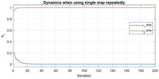
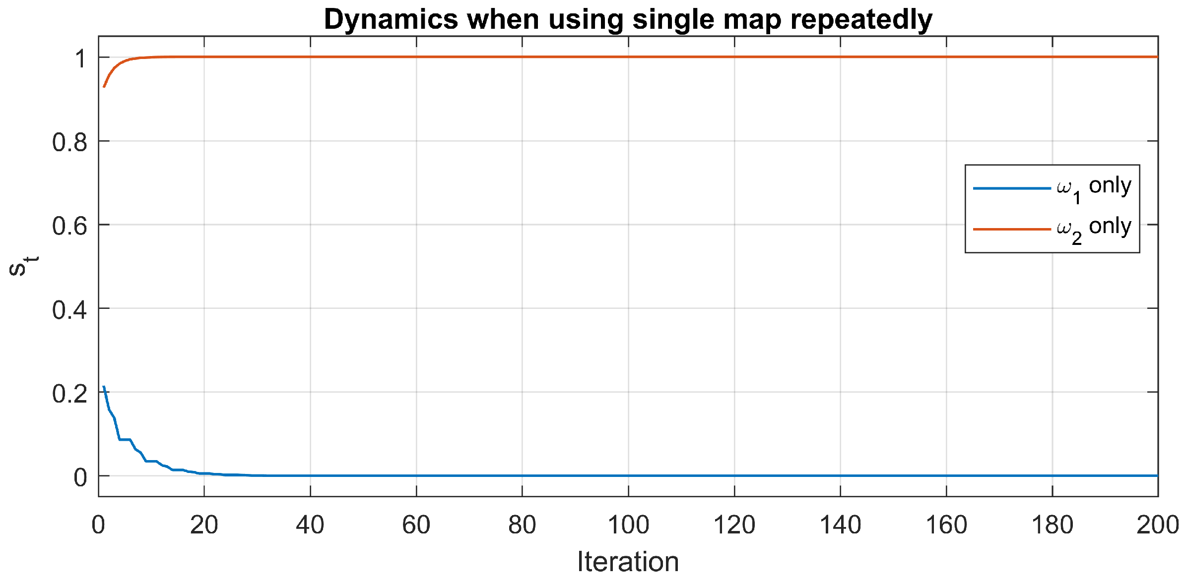
Figure 1 establishes the system’s fundamental stability and contractivity, showing that the individual application of ${\omega }_1$ drives the orbit to the fixed point 0, while ${\omega }_2$ drives it to 1.

Figure 1. Plots of the scalar outputs over iterations.

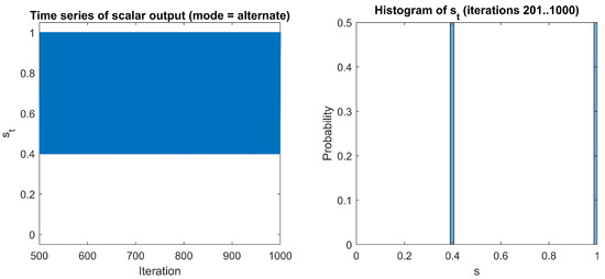
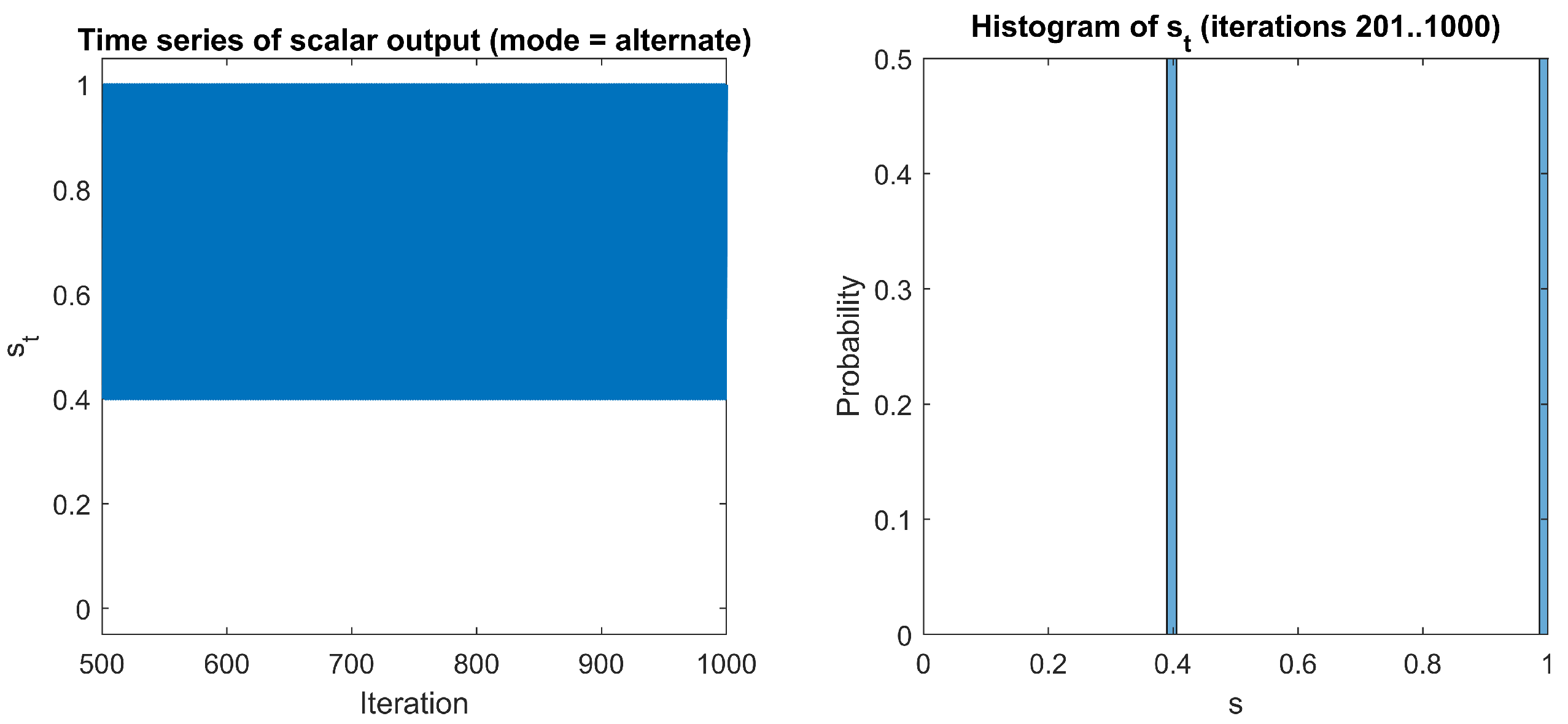
Figure 2 displays the alternating-mode dynamics, proving the attractor is a disjoint set rather than a continuous interval. The histogram’s two concentrated probability spikes, separated by a wide region of zero mass, empirically refute the uniform distribution expected from $[0,1]$.

Figure 2. Histogram of the last part of the orbit (approximate attractor distribution).

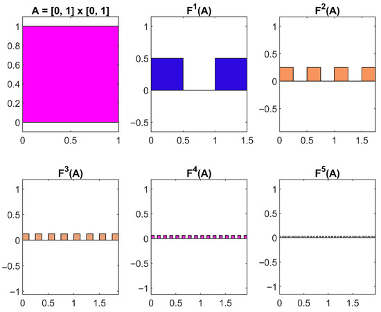
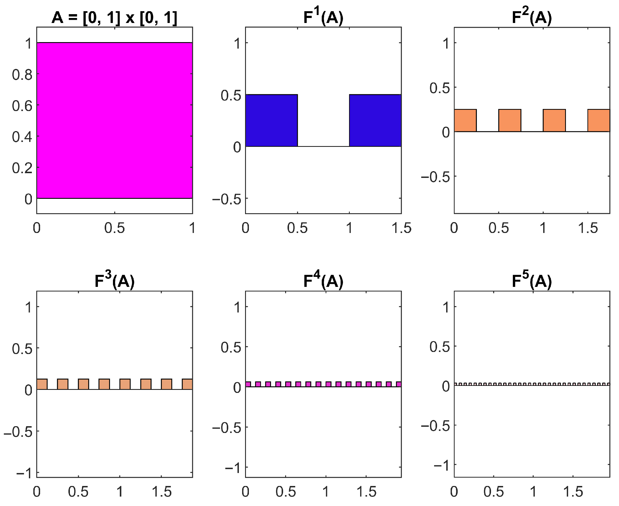
Figure 3 most conclusively depicts the iterative application of the set operator $\mathcal{S}$ and its hallmark feature, the self-similar fragmentation of the initial set. The panel-by-panel sequence visually confirms the rapid $\mathcal{S}$-convergence: the initial set A is immediately split into two disjoint components in $F^1\left(A\right)$, which are then recursively partitioned into four, eight, and sixteen smaller segments in subsequent iterations ($F^2\left(A\right)$ to $F^4\left(A\right)$). This sequence demonstrates the rapid shrinking and separation of points, confirming the system’s convergence to a Cantor-like fractal structure and thereby correcting the initial analysis that identified the attractor as the solid interval $[0,1]$.

Figure 3. Fractal geometrical presentation.

6. Conclusions and Future Perspectives

This study extends the framework of $(\mathcal{L};\mathcal{Y})$-contractions to product spaces $X^{\left|I\right|}$ and establishes new fixed point theorems under broader and more flexible assumptions. The proposed formulation generalizes classical results such as those of Banach, Boyd—Wong, Geraghty, and Wardowski, unifying them within a single analytical structure suited for nonlinear and coupled operator systems.

Using the Hausdorff—Pompeiu metric and the Hutchinson—Barnsley operator, a connection was developed between fixed point theory and fractal geometry through generalized iterated function systems (IFSs) formed by families of $(\mathcal{L};\mathcal{Y})$-contractions. The established results ensure the existence and uniqueness of fractal attractors and provide constructive iterative schemes for their approximation, linking theoretical rigor with computational practicality.

The framework has diverse applications: in dynamical systems, it offers tools for analyzing stability and convergence; in computer graphics and image processing, it supports the controlled generation of self-similar fractal structures; and in applied modeling, it aids the study of nonlinear equilibria and recursive processes in physics, biology, and economics. Future extensions may include multivalued and random IFSs, fuzzy or probabilistic metric formulations, and hybrid contraction models based on measures of noncompactness or integral inequalities. Overall, this work establishes a unified and adaptable foundation that bridges fixed point theory, fractal geometry, and nonlinear analysis, offering both theoretical advancement and practical applicability.

7. Open Problems

• The existence of fractal in Theorem 10 relies on compactness assumptions (C1) or relative compactness (C2). An open problem is to determine whether these results can be extended to settings where compactness is replaced by weaker topological conditions (e.g., closed and bounded sets in noncompact spaces).
• The fractal obtained through generalized $(\mathcal{L};\mathcal{Y})$-IFSs present opportunities for studying their Hausdorff dimension, measure-theoretic properties, and multifractal analysis, which remain open for further exploration.

References

- Banach, S. Sur les opérations dans les ensembles abstraits et leur application aux équations intégrales. Fundam. Math. 1922, 3, 133–181. [Google Scholar] [CrossRef] [Scilit]
- Amini-Harandi, A.; Petrusel, A. A fixed point theorem by altering distance technique in complete metric spaces. Miskolc Math. Notes 2013, 14, 11–17. [Google Scholar] [CrossRef] [Scilit]
- Browder, F.E. On the convergence of successive approximations for nonlinear functional equations. Indag. Math. 1968, 30, 27–35. [Google Scholar] [CrossRef] [Scilit]
- Rakotch, E. A note on contractive mappings. Proc. Am. Math. Soc. 1962, 13, 459–465. [Google Scholar] [CrossRef]
- Proinov, P.D. Fixed point theorems for generalized contractive mappings in metric spaces. J. Fixed Point Theory Appl. 2020, 22, 21. [Google Scholar] [CrossRef] [Scilit]
- Chanda, A.; Garai, H.; Dey, L.K. (L;M)-Wardowski contraction pairs and some applications. Comp. Appl. Math. 2021, 40, 294. [Google Scholar] [CrossRef] [Scilit]
- Nashine, H.K.; Saluja, G.S.; Ibrahim, R.W. Some fixed point theorems for -almost weak contractions in S-metric spaces solving conformable differential equations. J. Inequal. Appl. 2020, 2020, 139. [Google Scholar] [CrossRef] [Scilit]
- Karapınar, E.; Fulga, A. A fixed point theorem for Proinov mappings with a contractive iterate. Appl. Math. J. Chin. Univ. 2023, 38, 403–412. [Google Scholar] [CrossRef] [Scilit]
- Wasey, A.; Mior Othman, W.A.; Alshaban, E.; Wong, K.B.; Alatawi, A. Proinov-type relational contractions and applications to boundary value problems. Aims Math. 2025, 10, 13393–13408. [Google Scholar] [CrossRef] [Scilit]
- Nadler, S.B. Multi-Valued Contraction Mappings. Pacific J. Math. 1969, 30, 475–488. [Google Scholar] [CrossRef] [Scilit]
- Altun, I.; Minak, G. Multivalued F-contractions on Complete Metric Spaces. J. Nonlinear Convex Anal. 2015, 16, 659–666. [Google Scholar] [CrossRef] [Scilit]
- Ćirić, L. Multi-valued nonlinear contraction mappings. Nonlinear Anal. 2009, 71, 2716–2723. [Google Scholar] [CrossRef] [Scilit]
- Mizoguchi, N.; Takahashi, W. Fixed point theorems for multivalued mappings on complete metric spaces. J. Math. Anal. Appl. 1989, 141, 177–188. [Google Scholar] [CrossRef] [Scilit]
- Nashine, H.K.; Ibrahim, R.W.; Rhoades, B.E.; Pant, R. Unified Feng–Liu type fixed point theorems solving control problems. Rev. Real Acad. Cienc. Exactas F’Sicas Nat. Ser. Mat. (RACSAM) 2021, 115, 1–17. [Google Scholar] [CrossRef] [Scilit]
- Barnsley, M.F. Fractals Everywhere; Academic Press: Cambridge, MA, USA, 1988. [Google Scholar]
- Hutchinson, J. Fractals and self-similarity. Indiana Univ. Math. J. 1981, 30, 713–747. [Google Scholar] [CrossRef]
- Barnsley, M.F.; Demko, S. Iterated function systems and the global construction of fractals. Proc. Roy. Soc. Lond. Ser. A 1985, 399, 243–275. [Google Scholar]
- Chifu, C.; Petrusel, A. Multivalued fractals and generalized multivalued contractions. Chaos Solitons Fractals 2008, 70, 203–210. [Google Scholar] [CrossRef] [Scilit]
- Dung, N.V. Answers to questions on Ciric type theorems. Fractals 2017, 25, 1–9. [Google Scholar] [CrossRef] [Scilit]
- Llorens-Fuster, E.; Petrusel, A.; Yao, J.C. Iterated function systems and well-posedness. Chaos Solitons Fractals 2009, 41, 1561–1568. [Google Scholar] [CrossRef] [Scilit]
- Miculescu, R.; Mihail, A. Reich-type iterated function systems. J. Fixed Point Theory Appl. 2016, 18, 285–296. [Google Scholar] [CrossRef] [Scilit]
- Petrusel, A.; Soos, A. Self-similar sets and fractals generated by Ciric type operators. J. Nonlinear Sci. Appl. 2015, 8, 1048–1058. [Google Scholar] [CrossRef] [Scilit]
- Prithvi, B.V.; Katiyar, S.K. Interpolative operators: Fractal to multivalued fractal. Chaos Solitons Fractals 2022, 164, 112449. [Google Scholar] [CrossRef] [Scilit]
- Sahu, D.R.; Chakraborty, A.; Dubey, R.P. K-iterated function systems. Fractals 2010, 18, 139–144. [Google Scholar] [CrossRef] [Scilit]
- Singh, S.L.; Prasad, B.; Kumar, A. Fractals via iterated functions and multifunctions. Chaos Solitons Fractals 2009, 39, 1224–1231. [Google Scholar] [CrossRef] [Scilit]
- Xu, S.; Cheng, S.; Zhou, Z.; Reich, S. Iterated function systems and well-posedness via fixed point theory. Fixed Point Theory Appl. 2015, 2015, 71. [Google Scholar] [CrossRef] [Scilit]
- Rhoades, B.E. A comparison of various definitions of contractive mappings. Trans. Am. Math. Soc. 1977, 226, 257–290. [Google Scholar] [CrossRef]
- Dung, N.V.; Petrusel, A. On iterated function systems consisting of Kannan maps, Reich maps, Chatterjea type maps, and related results. J. Fixed Point Theory Appl. 2017, 19, 2271–2285. [Google Scholar] [CrossRef] [Scilit]
- Secelean, N.A. Countable Iterated Function Systems; Lambert Academic Publishing: Cambridge, MA, USA, 2013. [Google Scholar]
- Secelean, N.A. The existence of the attractor of countable iterated function systems. Mediterr. J. Math. 2012, 9, 61–79. [Google Scholar] [CrossRef] [Scilit]
- Hata, M. On some properties of set-dynamical systems. Proc. Jpn Acad. Ser. A 1985, 61, 99–102. [Google Scholar] [CrossRef] [Scilit]
- Wicks, K.R. Fractals and Hyperspaces; Lecture Notes in Mathematics; Springer: Berlin/Heidelberg, Germany, 1991; Volume 1492. [Google Scholar]
- Fernau, H. Infinite Iterated Function Systems. Math. Nachr. 1994, 170, 79–91. [Google Scholar] [CrossRef] [Scilit]
- Secelean, N.A. Iterated function systems consisting of F-contractions. Fixed Point Theory Appl. 2013, 277, 13. [Google Scholar] [CrossRef] [Scilit]
- Gwózdz-Lukawska, G.; Jachymski, J. IFS on a metric space with a graph structure and extensions of the Kelisky-Rivlin theorem. J. Math. Anal. Appl. 2009, 356, 453–463. [Google Scholar] [CrossRef] [Scilit]
- Pasupathi, R.; Navascues, M.A.; Chand, A.K.B. Iterated functions systems composed of generalized θ-contractions. Fractal Fract. 2021, 5, 69. [Google Scholar] [CrossRef] [Scilit]
- Dumitru, D. Generalized iterated function systems containing Meir-Keeler functions. An. Univ. Bucuresti Math. 2009, 58, 3–15. [Google Scholar]
- Strobin, F.; Swaczyna, J. On a certain generalization of the iterated function system. Bull. Aust. Math. Soc. 2013, 87, 37–54. [Google Scholar] [CrossRef] [Scilit]
- Cui, M.; Selmi, B.; Li, Z. Expansive measures of nonautonomous iterated function systems. Qual. Theory Dyn. Syst. 2025, 24, 60. [Google Scholar] [CrossRef] [Scilit]
- Thangaraj, C.; Easwaramoorthy, D.; Selmi, B.; Chamola, B.P. Generation of fractals via iterated function system of Kannan contractions in controlled metric space. Math. Comput. Simul. 2024, 222, 188–198. [Google Scholar] [CrossRef] [Scilit]
- Secelean, N.A. Generalized F-iterated function systems on product of metric spaces. J. Fixed Point Theory Appl. 2015, 17, 575–595. [Google Scholar] [CrossRef] [Scilit]
- Moradi, S. Fixed point of single-valued cyclic weak YF -contraction mappings. Filomat 2014, 28, 1747–1752. [Google Scholar] [CrossRef] [Scilit]
- Geraghty, M.A. On contractive mappings. Proc. Am. Math. Soc. 1973, 40, 604–608. [Google Scholar] [CrossRef]
- Jleli, M.; Samet, B. A new generalization of the Banach contraction principle. J. Inequal. Appl. 2014, 2014, 1–8. [Google Scholar] [CrossRef] [Scilit]
- Ahmad, J.; Al-Mazrooei, A.E.; Cho, Y.J.; Yang, Y.O. Fixed point results for generalized θ-contractions. J. Nonlinear Sci. Appl. 2017, 10, 2350–2358. [Google Scholar] [CrossRef] [Scilit]
- Li, Z.; Jiang, S. Fixed point theorems of JS-quasi-contractions. Fixed Point Theory Appl. 2016, 2016, 40. [Google Scholar] [CrossRef] [Scilit]
- Wardowski, D. Fixed points of a new type of contractive mappings in complete metric spaces. Fixed Point Theory Appl. 2012, 2012, 94. [Google Scholar] [CrossRef] [Scilit]
- Secelean, N.A. Weak F-contractions and some fixed point results. Bull. Iranian Math. Soc. 2016, 42, 779–798. [Google Scholar]
- Piri, H.; Kumam, P. Some fixed point theorems concerning F-contraction in complete metric spaces. Fixed Point Theory Appl. 2014, 2014, 210. [Google Scholar] [CrossRef] [Scilit]
- Lukács, A.; Kajánto, S. Fixed point theorems for various types of Fcontractions in complete b-metric spaces. Fixed Point Theory 2018, 19, 321–334. [Google Scholar] [CrossRef] [Scilit]
Disclaimer/Publisher’s Note: The statements, opinions and data contained in all publications are solely those of the individual author(s) and contributor(s) and not of MDPI and/or the editor(s). MDPI and/or the editor(s) disclaim responsibility for any injury to people or property resulting from any ideas, methods, instructions or products referred to in the content. |
© 2026 by the authors. Licensee MDPI, Basel, Switzerland. This article is an open access article distributed under the terms and conditions of the Creative Commons Attribution (CC BY) license.