


Abstract
For the hierarchical normal and normal-inverse-gamma model, we derive the Bayesian estimator of the variance parameter in the normal distribution under Stein’s loss function—a penalty function that treats gross overestimation and underestimation equally—and compute the associated Posterior Expected Stein’s Loss (PESL). Additionally, we determine the Bayesian estimator of the same variance parameter under the squared error loss function, along with its corresponding PESL. We further develop empirical Bayes estimators for the variance parameter using a conjugate normal-inverse-gamma prior, employing both the method of moments and Maximum Likelihood Estimation (MLE). Theoretical properties, including posterior and marginal distributions, two inequalities that relate two Bayes estimators and their corresponding PESLs, and consistencies of hyperparameter estimators and empirical Bayes estimators, are established. The simulation results demonstrate that MLEs outperform moment estimators in estimating hyperparameters, particularly with respect to consistency and model fit. Finally, we apply our methodology to real-world data on poverty levels—specifically, the percentage of individuals living below the poverty line—to validate and illustrate our theoretical findings.
Keywords:
empirical Bayes estimators; hierarchical normal and normal-inverse-gamma model; Maximum Likelihood Estimation (MLE) method; moment method; Stein’s loss function MSC:
62C12; 62F10; 62F15
1. Introduction
The empirical Bayes method depends on a conjugate prior modeling, where the hyperparameters are estimated from the observations, and the “estimated prior” is then used as a regular prior in the subsequent inference. See [1,2,3] and the references therein. The empirical Bayes method is introduced in [4,5,6]. From a Bayesian perspective, it means that the sampling distribution is known, but the prior distribution is not. The marginal distribution is then used to restore the prior distribution from the observations. More literature on the empirical Bayes method can be found, for instance, in [7,8,9,10,11,12,13,14,15,16,17,18,19,20,21,22,23,24].
The motivations of this paper are summarized as follows. Example 1.5.1 (p. 20) of [25], Part I (pp. 69–70) of [26], and [19] have considered the following hierarchical normal and normal-inverse-gamma (N-NIG) model:
where , , , and are known hyperparameters, and iid means independent and identically distributed. The distribution is a joint conjugate prior for of the normal distribution , so that the posterior distribution of is an distribution with updated hyperparameters. However, in reality, the hyperparameters are unknown. Ref. [19] have estimated the hyperparameters of the model (1) by the moment method and the Maximum Likelihood Estimation (MLE) method. Moreover, they obtained the Bayes estimators of the mean and variance parameters of the model (1) under the squared error loss function. Finally, they obtained the empirical Bayes estimators of the mean and variance parameters of the model (1) under the squared error loss function by the moment method and the MLE method. However, in their empirical Bayes estimators, the samples have been used twice. First, the samples are utilized to estimate the hyperparameters , , , and . Second, the samples are used to obtain the Bayes estimators. To avoid using the sample twice, and to be compatible with the usual empirical Bayes analysis, we will use the following hierarchical N-NIG model in this paper:
where , , , and are hyperparameters to be determined, and are the unknown parameters of interest, is a normal distribution with an unknown mean and an unknown variance , the conditional conjugate prior distribution of given is which is a normal distribution with mean and an unknown variance , the marginal conjugate prior distribution of is which is an inverse gamma distribution with shape parameter and scale parameter . Note that the joint conjugate prior is a normal-inverse-gamma distribution. A notation table for the hyperparameter symbols, with their explicit role statement can be found in Table 1. As described in [7], the statistician observes data and wishes to make an inference about and . Therefore, provides direct information about the parameters and , while supplementary information is also available. The connection between the prime datum and the supplementary information is provided by the common distributions , , and . Moreover, since the variance parameter of the normal distribution is a positive restricted parameter, the squared error loss function is not appropriate. In contrast, we will choose Stein’s loss function because it penalizes gross overestimation and gross underestimation equally, that is, an action a will incur an infinite loss when it tends to 0 or ∞. Note that the squared error loss function does not have this property. For more literature on Stein’s loss function, we refer readers to [20,27,28,29,30].
Table 1.
A notation table for the hyperparameter symbols, with their explicit role statement.
The key contributions of this work are outlined below. For the hierarchical N-NIG model (2), we begin by deriving the posterior distributions and marginal density, as stated in Theorem 1. Subsequently, we derive Bayes estimators for the variance parameter of the normal distribution under two loss criteria: Stein’s loss and the squared error loss. We further compute the corresponding Posterior Expected Stein’s Losses (PESLs) associated with these two estimators. It is shown that the two Bayes estimators and their respective PESLs satisfy specific inequalities, namely (13) and (14) (Theorem 2). Additionally, we derive moment-based estimators for the hyperparameters of the hierarchical N-NIG model (2) and establish their consistency in Theorem 3. Similarly, Maximum Likelihood Estimators (MLEs) for the same hyperparameters are derived, and their consistency is proven in Theorem 4. Building on these results, Theorem 5 provides the consistencies of the empirical Bayes estimators of under Stein’s loss function using the moment and MLE methods. The theoretical findings are supported by numerical experiments and an application to real-world data.
Comparing models (1) and (2) carefully, we find that the samples and generated from the two models are iid from different distributions. On the one hand, the sample generated from (1) are iid from . Although the marginal densities of are , and thus can be thought to be from the t distribution. However, are not iid from the t distribution. In other words, are dependent from the t distribution. On the other hand, the sample generated from (2) are iid from the t distribution. That is, are independent and identically distributed from the t distribution. The sample can be used to estimate the parameters and from , while the sample can be used to estimate the hyperparameters , , and from , where .
The structure of this paper is outlined as follows. Section 2 begins with the derivation of posterior distributions and the marginal likelihood for the hierarchical N-NIG model (Theorem 1). Subsequently, we derive the corresponding Bayes estimators and PESLs, which are shown to fulfill two key inequalities: (13) and (14) (Theorem 2). Additionally, Theorem 3 provides moment estimators of the hyperparameters and their consistencies. Theorem 4 provides MLEs of the hyperparameters and their consistencies. Moreover, Theorem 5 provides the consistencies of the empirical Bayes estimators of under Stein’s loss function using the moment and MLE methods. In Section 3, we conduct numerical experiments from eight different perspectives to evaluate performance. Section 4 illustrates the methodology using real-world data, specifically poverty rate data reflecting the proportion of individuals living below the poverty line. Finally, Section 5 offers a discussion of the findings and concluding remarks.
2. Theoretical Results
Suppose that follows a gamma distribution and follows an inverse gamma distribution. The probability density functions (pdfs) of X and Y are respectively given by
It is easy to calculate and , for and .
2.1. The Bayes Estimators and the PESLs
For the hierarchical N-NIG model (2), we have the following theorem which calculates the posterior densities , , , , and the marginal density . The proof of the theorem can be found in Appendix A.
Theorem 1.
For the hierarchical N-NIG model (2), the joint posterior density of is
the marginal posterior density of is
the marginal posterior density of is
the conditional posterior density of is
where
and
Moreover, the marginal density of is the density of a non-standardized Student t-distribution, given by
with probability density function (pdf) given by
for , , , , and .
In the following, we will calculate the Bayes estimator of under Stein’s loss function , the Bayes estimator of under the usual squared error loss function , and the PESLs at and ( and ). Stein’s loss function in terms of and a is given by
where . The usual squared error loss function in terms of and a is given by
where .
Similar to [28], the two Bayes estimators and the two PESLs are respectively given by
To calculate the two Bayes estimators and the two PESLs, it remains to calculate
Similar to [28], we present the following theorem concerning two inequalities that relate the two Bayes estimators and their corresponding PESLs. The proof of the theorem can be located in Appendix A.
Theorem 2.
For the two Bayes estimators, we obtain the following result
by applying Jensen’s inequality. Additionally, for the two PESLs, we obtain the following result
which is a direct consequence of the general methodology for finding a Bayes estimator. According to construction, minimizes the Posterior Expected Stein’s Loss (PESL).
Now let us analytically calculate the Bayes estimators and , and the PESLs and under the hierarchical N-NIG model (2) from (9) to (12). The three expectations are calculated as
for , where and are given by (4) and (5). From (9), the Bayes estimator of under Stein’s loss function is given by
From (10), the Bayes estimator of under the usual squared error loss function is given by
for . It is easy to show that
which exemplifies the theoretical study of (13). Furthermore, from (11) and (12), the PESL at and are respectively given by
and
where
is the digamma function. It can be shown that
which exemplifies the theoretical study of (14). It is worth noting that the PESLs and depend only on , but not on . Therefore, the PESLs depend only on , but not on , , , and .
2.2. The Empirical Bayes Estimators of
In this subsection, we will examine the consistencies of estimators for hyperparameters. Additionally, we will examine the consistencies of empirical Bayes estimators.
2.2.1. Consistencies of Estimators of Hyperparameters
In this subsubsection, we will show consistencies of estimators of hyperparameters.
The hyperparameters of Model (2) are , , , and . However, we can not directly obtain the estimators of the four hyperparameters of Model (2) by the moment method. Let
Since and appear together in , we can not directly obtain the estimators of and by the moment method. In other words, and are unidentifiable. In the empirical Bayesian statistical literature, common approaches to addressing the issue of unidentifiability of hyperparameters include the following two. One is to estimate the prior distribution through non-parametric or semi-parametric methods, avoiding strong assumptions about the functional form of the prior distribution, thereby circumventing the problem of unidentifiability of hyperparameters [31,32]. The other is to use auxiliary data, model structure constraints, or specific assumptions (such as sparsity and spatial correlation) to provide additional information, making the unidentifiable hyperparameters identifiable [33,34,35]. We adopt the second approach to make hyperparameters ( and ) identifiable. More specifically, when is fixed to be a known constant (our recommendation is , which will be made clear later in the next subsubsection), then and are identifiable. Otherwise, and are unidentifiable.
However, we can obtain the estimator of by the moment method. In the following, we are interested in the hyperparameters , , and . Using hyperparameters , , and , the marginal density (6) changes to
The moment-based estimators for the hyperparameters , , and in Model (2), denoted as , , and , along with their consistency properties, are presented in the subsequent theorem. The proof of this theorem is provided in Appendix A. To ensure the theorem holds, three conditions must be satisfied:
- (A1).
- Model specification: The observations are independently and identically distributed according to the marginal distribution of Model (2), i.e., for ,
- (A2).
- Moment of existence: The degrees-of-freedom parameter satisfies , so that the first four moments of exist and are finite.
- (A3).
- Well-definedness of estimators: The sample moments
Theorem 3 (Method of moments estimators and their consistencies).
Consider the hierarchical N-NIG model (2). Suppose the conditions (A1)–(A3) are satisfied, then the method of moments estimators for the hyperparameters , , and are given by
Moreover, these estimators are consistent, i.e.,
as the sample size n tends to infinity, where denotes convergence in probability.
For Theorem 3, we have the following remarks.
Remark 1.
Condition (A1) guarantees that the data-generating process agrees with the theoretical model. Condition (A2) ensures that the sample moments converge to their population counterparts, which is necessary for consistency. Condition (A3) avoids division by zero in the estimators; for large n, this is almost always satisfied. The quantity is identifiable even though and are not separately identifiable. In practice, we recommend to obtain a unique estimate of (see Section 2.2.2).
Remark 2.
The moment estimators , , and in Theorem 3 are the same as those in Theorem 2 in [19]. The reason for the same moment estimators is that for the two hierarchical N-NIG models (1) and (2), the marginal distributions are the same, and the population moments of X are the same. Moreover, in Theorem 3 of this paper, we have shown that the moment estimators are consistent estimators of the hyperparameters, and this result has not been derived in [19].
The MLE method is used to derive estimators for the hyperparameters , , and of Model (2), denoted as , , and , respectively. The consistency properties of these estimators are presented in the subsequent theorem, with the detailed proof provided in Appendix A. To ensure the theorem holds, five conditions must be satisfied:
- (B1).
- Model specification: Let the observations be independent and identically distributed according to the marginal Student-t distribution derived from (2), i.e., for ,
- (B2).
- Parameter space: , , and .
- (B3).
- Identifiability: is fixed at a known positive constant (we recommend in practice, and the reasons are given in Section 2.2.2), rendering the hyperparameters identifiable.
- (B4).
- Differentiability: The log-likelihood functionis twice continuously differentiable in a neighborhood of the true parameter values, and the expected Fisher information matrix is positive definite.
- (B5).
- Unique solution: The system of score equations
Theorem 4 (Consistency of Maximum Likelihood Estimators).
The MLEs of the hyperparameters , , and cannot be derived analytically by solving equations (24)–(26). As a result, numerical methods must be employed. Newton’s method can be applied to solve these equations and thereby obtain the MLEs of the hyperparameters. It should be emphasized that the accuracy of the resulting MLEs is highly sensitive to the choice of initial values, and moment-based estimators have generally been found to serve as effective starting points.
2.2.2. Consistencies of Empirical Bayes Estimators
In this subsubsection, we will show consistencies of empirical Bayes estimators.
First, let us discuss the selection of . We recommend choosing , and the reason is given as follows. From (18), (4), and (5), we have
It is easy to show that the factor
for . Because we have little information about , we will choose
which is in the middle of the above range. Hence,
Therefore, (27) reduces to
which can then be estimated once the hyperparameters are estimated. From (22) and (28), we have
which can then be estimated once the hyperparameter is estimated.
Another reason to choose is given below. Since , the squared error loss function is appropriate. The Bayes estimator of under the squared error loss function is given by
In (29), represents a strength of belief on . If one harbors no belief on , then , and thus , which depends only on the datum . In contrast, if one harbors complete belief on , then , and thus , which depends only on . However, if one believes that and are equally important, then is a reasonable choice, and thus , which is a balanced combination of and .
We remark that and affect , , , and , and they do not affect , , and .
Let , , and be moment estimators (calculated in Theorem 3) of , , and , respectively. Let , , and be MLEs (numerically determined in Theorem 4) of , , and , respectively. Inspired by (27) and (28), let
be the empirical Bayes estimator of under Stein’s loss function by the moment method, let
be the empirical Bayes estimator of under Stein’s loss function by the MLE method, let
be the Bayes estimator of under Stein’s loss function by the oracle method, and let
be the Bayes estimator of under Stein’s loss function with a fixed , which is our primary object of interest.
From Theorems 3 and 4, we have the following theorem regarding the consistencies of the empirical Bayes estimators of under Stein’s loss function by the moment and MLE methods. The detailed proof of the theorem is provided in Appendix A.
Theorem 5.
Under the conditions of Theorems 3 and 4, we have for all ,
and
Note that,
In addition, is an increasing function of . More specifically,
In other words, will underestimate , and it will overestimate . A schematic plot of the empirical Bayes estimators and Bayes estimators is graphed in Figure 1.
Figure 1.
A schematic plot of the empirical Bayes estimators (EBEs) and Bayes estimators (BEs).
2.3. Comparison of Loss Functions, Posterior Risks, and Corresponding Bayes Estimators
In this subsection, a comparison will be conducted between two loss functions, namely Stein’s loss function and the power-power loss function. Additionally, a comparison will be made between two posterior risks, and . Moreover, a comparison will be carried out between two Bayes estimators, and . Finally, a comparison will be performed between the two posterior risks evaluated at the two Bayes estimators.
First, we shall compare the two loss functions. Stein’s loss function with respect to and a is presented as (7). The power-power loss function (refer to [36]) with respect to and a is defined as
A comprehensive comparison of the two loss functions can be found in [36]. As elaborated in [36], both functions are suitable loss functions in the domain . Specifically, the two loss functions impose equal penalties on gross overestimation and gross underestimation. That is to say, an action a will result in an infinite loss when it approaches 0 or ∞. In comparison with Stein’s loss function, the power-power loss function has an additional characteristic: it has balanced convergence rates or penalties for cases where its argument is either too large or too small.
Second, let us conduct a comparison between the two posterior risks. The posterior Stein’s risk, denoted as , is defined as follows:
The posterior power-power risk, also known as the Posterior Expected Power-power Loss (PEPL), is represented by , and is given by:
Third, let us compare the two Bayes estimators. From [28], the Bayes estimator minimizes the PESL, , that is,
where is the action space, is an action (estimator). Similarly, from [36], the Bayes estimator minimizes the PEPL, , that is,
By applying a similar technique as that utilized in [36], it can be demonstrated that
3. Simulations
This section presents numerical simulations for the hierarchical N-NIG model (2). We examine eight key aspects: (1) model comparison and estimator performance; (2) the consistencies of moment estimators and MLEs; (3) the influence of on quantities of interest as functions of ; (4) the validity of two inequalities concerning Bayes estimators and PESLs; (5) the model’s goodness-of-fit to the generated data; (6) the examination of the model’s marginal densities; (7) comparison with standard MLE under PESL; and (8) comparison of loss functions, posterior risks, and corresponding Bayes estimators.
The simulated data are generated according to the hierarchical N-NIG model (2) with the hyperparameters specified by , , , and . The reason why we choose these values is that , , , and . Moreover, is required in moment estimations of the hyperparameters. Additional numerical values for the hyperparameters can likewise be defined.
3.1. Model Comparison and Estimator Performance
This subsection aims to numerically compare two hierarchical N-NIG models (1) and (2) in estimating hyperparameters. It demonstrates that samples from Model (1) fail to estimate correctly, while samples from Model (2) succeed. Additionally, the subsection evaluates the performance of the method of moments and MLE, highlighting that both can accurately recover regardless of the specific values of and .
First, we will numerically exemplify that the sample generated from Model (1) can not be used to estimate the hyperparameters , while the samples and generated from Model (2) can be used to estimate the hyperparameters , where . Moreover, we will exemplify that the moment estimators and the MLEs of can correctly estimate the true hyperparameter regardless of the and values.
Below is a detailed description of the simulation settings and the data generation process for the three samples (), along with the computational steps for the estimators.
Simulation Setup and Data Generation
All simulations use a fixed sample size of . The true hyperparameters are set as , , and the derived .
- 1.
- Generation of from Model (1):
- -
- Draw a single variance parameter: .
- -
- Draw a single mean parameter conditional on : .
- -
- Generate n independent observations: for .
- 2.
- Generation of from Model (2) with :
- -
- For each :
- a.
- Draw a variance parameter: .
- b.
- Draw a mean parameter conditional on : .
- c.
- Generate an observation: .
- -
- The marginal distribution of each is with .
- 3.
- Generation of from Model (2) with :
- -
- For each :
- a.
- Draw a variance parameter: .
- b.
- Draw a mean parameter conditional on : .
- c.
- Generate an observation: .
- -
- The marginal distribution of each is with .
Computation of the Estimators
- 1.
- Method of Moments Estimators (Theorem 3): The estimators , , and are computed directly from the first, second, and fourth sample moments of the observed data .
- -
- Calculate the sample moments:
- -
- The moment estimators , , and are computed as in Theorem 3.
- 2.
- Maximum Likelihood Estimators (Theorem 4): The MLEs , , and are obtained by solving the system of score Equations (24)–(26) numerically via Newton’s method.
- -
- The log-likelihood function for , , and is:
- -
- -
- Newton’s Method: Let . The iterative update is:
The histograms of the samples and their density curves are plotted in Figure 2. From the figure, we observe the following facts.
- 1.
- Plot (a): the sample generated from (1) are iid from with and .
- 2.
The moment estimators and the MLEs of the hyperparameters for the samples , , and are summarized in Table 2. From the table, we observe the following facts.
Table 2.
The moment estimators and the MLEs of the hyperparameters for the samples , , and .
- 1.
- The moment estimators of the hyperparameters for sample are far away from the true hyperparameters , and thus the samples generated from the model (1) can not be used to estimate the hyperparameters .
- 2.
- For , since the moment estimator of is , which is negative, the MLE method fails to iterate, and thus the MLEs of the hyperparameters are equal to the moment estimators.
- 3.
- For and , the moment estimators and the MLEs of the hyperparameters are close to the true hyperparameters , and thus the samples generated from Model (2) can be used to estimate the hyperparameters .
- 4.
- 5.
- For and , the MLEs are closer to the true hyperparameters than the moment estimators for this simulation.
3.2. Consistencies of the Moment Estimators and the MLEs
In this subsection, we will numerically illustrate two kinds of consistencies of the moment estimators and the MLEs. One is consistency of estimators of hyperparameters, and the other is consistency of empirical Bayes estimators.
3.2.1. Consistencies of Estimators of Hyperparameters
Currently, both the moment estimators and the MLEs serve as consistent estimates for the hyperparameters of the hierarchical N-NIG model (2). The purpose of this subsubsection is to emphasize that, as established in Theorems 3 and 4, we have rigorously proven the consistencies of both the moment-based and MLE-based estimators with respect to the true hyperparameters. It should be noted that all analyses here are based solely on the observed data .
Following the approach in [21], let represent one of the hyperparameters , , or . Consistency is defined as the property that
for , where corresponds to the moment estimator and to the MLE, with denoting convergence in probability and n being the sample size. Equivalently, consistency can be expressed as
for any and for all . These probabilities are estimated using empirical frequencies from simulations:
where is the indicator function taking value 1 if event A occurs and 0 otherwise, and M denotes the number of simulation replications. Hence, a decreasing trend in the simulated frequencies toward zero as n increases provides empirical evidence of estimator consistency, for both estimation methods () and across all hyperparameters .
We now demonstrate that the moment estimators and the MLEs are consistent estimators of the hyperparameters . Table 3 presents the frequency distributions of these estimators for both moment-based and MLE for varying sample sizes n, under settings where , , and . The simulated data are generated from the hierarchical N-NIG model (2), with hyperparameter values set to and . While other configurations of these hyperparameters could also be considered, the current choice serves to illustrate the behavior effectively. Analysis of the table reveals several key observations.
Table 3.
The frequencies of the moment estimators and the MLEs of the hyperparameters as n varies for , , and .
- 1.
- With , , or , the frequencies of the estimators approach zero as n tends to infinity, indicating that both the moment estimators and the MLEs are consistent for estimating the hyperparameters. In the case of , the frequencies of and remain relatively high (at least across all scenarios). Nevertheless, a decreasing trend toward zero is evident as n grows large, suggesting eventual convergence.
- 2.
- By comparing the frequencies corresponding to , , and , we find that as decreases, the frequencies generally increase. This occurs because the constraintsbecome easier to satisfy when is smaller.
- 3.
- While small samples (e.g., ) result in relatively high error frequencies, MLEs consistently achieve lower frequencies than moment estimators for and across all sample sizes, and for once the sample size becomes moderately large (e.g., ). This indicates that, in terms of convergence, MLEs offer more reliable estimation of the hyperparameters, particularly with larger samples.
3.2.2. Consistencies of Empirical Bayes Estimators
The purpose of this subsubsection is to emphasize that, as established in Theorem 5, we have rigorously demonstrated the consistencies of both the moment-based and MLE-based estimators with respect to . It is important to note that all analyses herein are based on the observed data .
To illustrate (30) and partially illustrate Theorem 5, we generate
where are iid generated from (2) for and (, 1e3, and 1e4). Note that
where , , and ( and ). The histogram of are displayed in Figure 3. From this figure, we observe that the data are roughly symmetric around its mean . Note that in (37), for each prime datum , there is only one supplementary information .
Figure 3.
The histogram of , where and 1e4.
, , , , , and as functions of for , 1e3, and 1e4 are displayed in Figure 4. In this figure, red ∘ corresponds to , blue △ corresponds to 1e3, and purple + corresponds to 1e4. From this figure, we observe the following facts.
Figure 4.
, , , , , and as functions of for , 1e3, and 1e4.
- 1.
- For plots (a) and (b), the y-axis range is . The three scatterplots corresponding to with appear closely clustered. Among the empirical Bayes estimators, and for (red ∘) exhibit the widest spread, those for 1e3 (blue △) are more concentrated, and the results for 1e4 (purple +) are largely obscured by the three scatterplots of with .
- 2.
- For plots (c) and (d), the y-axis range is . These plots show that the empirical Bayes estimators and are most widely dispersed for (red ∘), become more concentrated for 1e3 (blue △), and are most concentrated for 1e4 (purple +). As n increases, the empirical Bayes estimates converge toward the limiting oracle estimator , which coincides with the estimator . Indeed, the scatterplots of these two estimators ( and ) overlap completely. Furthermore, the oracle estimator systematically underestimates and overestimates . The two plots illustrate (30).
- 3.
- A comparison between plots (c) and (d) reveals that for 1e3 and 1e4, the estimates based on are more tightly clustered around the oracle estimator than those based on . This indicates that the MLE method outperforms the method of moments when the sample size is moderately large (e.g., 1e3 and 1e4).
To further illustrate Theorem 5, we generate
where are iid generated from (2) for and (, 1e3, 1e4, 2e4, 4e4, 8e4, and 16e4). is fixed to be 3 or 4. The simulated data are generated from the hierarchical N-NIG model (2), with hyperparameter values set to and . While alternative configurations of these hyperparameters can also be taken into account, the present selection effectively demonstrates the behavior. Under this hyperparameter setting, it is easy to show that . Therefore, and 4 are two typical values of . Note that in (38), for the prime datum , there are M supplementary information for .
Let
Then, by Theorem 5, we have
for , where corresponds to the moment estimator and to the MLE, with denoting convergence in probability and n being the sample size.
Boxplots of and for different sample sizes n are plotted in Figure 5. From this figure, we observe the following facts.
Figure 5.
Boxplots of and for different sample sizes n when (a,b) and (c,d). The gray horizontal line is .
- 1.
- When sample sizes n increases, the variances of and become smaller, and the empirical Bayes estimators tend to . This indicates that and are consistent estimators of for and 4.
- 2.
- Numerical results display that when , the interquartile ranges by the moment method are 0.5363, 0.2313, 0.0804, 0.0651, 0.0466, 0.0473, and 0.0290, those by the MLE method are 0.5361, 0.1995, 0.0389, 0.0257, 0.0176, 0.0138, and 0.0098, for seven sample sizes, 1e3, 1e4, 2e4, 4e4, 8e4, 16e4; when , the interquartile ranges by the moment and MLE methods are respectively given by 0.5410, 0.2062, 0.0702, 0.0593, 0.0421, 0.0426, 0.0258 and 0.5090, 0.1758, 0.0346, 0.0230, 0.0137, 0.0131, and 0.0086, for the same seven sample sizes. This indicates that in terms of interquartile range, the MLE method consistently outperforms the moment method for the seven sample sizes.
We now demonstrate that the empirical Bayes estimators and are consistent estimators of . Table 4 presents the frequency distributions of these empirical Bayes estimators for both moment-based and MLE for varying sample sizes n, under settings where , , and . An analysis of the table uncovers several crucial observations.
Table 4.
The frequencies of the moment estimators and the MLEs of as n varies for , , and .
- 1.
- With , , or , the frequencies of the estimators approach zero as n tends to infinity, indicating that both the moment estimators and the MLEs are consistent for estimating .
- 2.
- By comparing the frequencies corresponding to , , and , we find that as decreases, the frequencies generally increase. This occurs because the constraintsbecome easier to satisfy when is smaller.
- 3.
- While small samples (e.g., ) result in relatively high error frequencies, MLEs consistently achieve lower frequencies than moment estimators for and once the sample size becomes moderately large (e.g., ). This indicates that, in terms of convergence, MLEs offer more reliable estimation of , particularly with larger samples.
3.3. The Effect of for Quantities of Interest as Functions of
In this subsection, we will investigate the effect of for quantities of interest (, , , , , , and ) as functions of . The motivation of this subsection is that is unidentifiable, and we want to know whether using (our recommendation) for the computation will overestimate or underestimate quantities of interest as functions of when the true (e.g., 2 or ) is different from .
Quantities of interest as functions of for in the simulations are plotted in Figure 6. In all the plots, is fixed. From the figure, we observe the following facts.
Figure 6.
Quantities of interest as functions of for in the simulations. is fixed in all the plots. Left column (a,c,e,g): , , , and are affected by . Right column (b,d,f): , , and are not affected by .
- 1.
- From the left column of the figure, we see that , , , and are affected by . Moreover, , , and are quadratic functions of (note that their y ranges are different), while is a linear function of .
- 2.
- For plot (a), we observe that when using will underestimate when using , and it will overestimate when using . In other words, is an increasing function of for a fixed . Similar phenomena are observed for (plot (c)) and (plot (e)).
- 3.
- For (plot (g)), we observe an interesting phenomenon that when ( in the simulation), when using will underestimate that when using , and it will overestimate that when using . In other words, is an increasing function of when . However, when , we observe a reversed phenomenon that when using will overestimate that when using , and it will underestimate that when using . In other words, is a decreasing function of when . The phenomena can be explained by the theoretical analysis of
- 4.
- From the right column of the figure, we see that , , and are not affected by . Moreover, they also do not depend on .
3.4. Two Inequalities of the Bayes Estimators and the PESLs
This subsection aims to provide numerical illustrations of the two inequalities related to the Bayes estimators and the PESLs—specifically, (20) and (21)—under the oracle scenario where the hyperparameters are known. The rationale for this subsection lies in the theoretical foundation established by two inequalities (13) and (14), which we seek to validate through numerical examples.
First, we fix , , , and . Then, we set a seed number 1 in R software and draw from . Next, we draw from . After that, we draw from . Figure 7 shows the histogram of and the density estimation curve of . It is that we find to minimize the PESL. Numerical results show that
and
which exemplify the theoretical studies of (20) and (21).
Figure 7.
The histogram of and the density estimation curve of .
We now consider the scenario where one of the five parameters—, , , , and —is allowed to vary while the others remain constant. Specifically, our focus lies on conducting a sensitivity analysis of the Bayes estimators and the PESLs with respect to these five parameters.
Figure 8 illustrates the Bayes estimators and the PESLs as varying with . As shown in the left panel, the Bayes estimators exhibit dependence on , demonstrating the validity of inequality (20). Specifically, increases as increases, whereas decreases with rising . The right panel reveals that the PESLs are also influenced by , supporting the inequality (21), and both PESLs decrease monotonically as grows. Additionally, numerical values corresponding to these quantities are provided in Table 5, which aligns with the graphical representation in Figure 8. Overall, both the figure and the table confirm the two theoretical inequalities: (20) and (21).
Figure 8.
The Bayes estimators and the PESLs as functions of . (a) Bayes estimators vs. . (b) PESLs vs. .
Table 5.
The numerical values of the Bayes estimators and the PESLs in Figure 8: changes.
Figure 9 shows the Bayes estimators and the PESLs as functions of , , , and . We see from the left plots of the figure that the Bayes estimators depend on , , , and , and (20) is exemplified. Moreover, the Bayes estimators are first decreasing and then increasing functions of and , and they are increasing functions of and . The right plots of the figure exhibit that the PESLs do not depend on , , , and , and (21) is exemplified. Furthermore, Table 6, Table 7, Table 8 and Table 9 display the numerical values of the Bayes estimators and the PESLs in Figure 9. In summary, the results of Figure 9 and Table 6, Table 7, Table 8 and Table 9 exemplify the two inequalities (20) and (21).
Figure 9.
The Bayes estimators and the PESLs as functions of , , , and . (a,c,e,g) Bayes estimators vs. , , , and . (b,d,f,h) PESLs vs. , , , and .
Table 6.
The numerical values of the Bayes estimators and the PESLs in Figure 9: changes.
Table 7.
The numerical values of the Bayes estimators and the PESLs in Figure 9: changes.
Table 8.
The numerical values of the Bayes estimators and the PESLs in Figure 9: changes.
Table 9.
The numerical values of the Bayes estimators and the PESLs in Figure 9: changes.
In brief, the results of Figure 8 and Figure 9 exemplify that the PESLs depend only on , but not on , , , and .
Since the estimators and , along with their corresponding PESLs— and —are functions of the parameters and , where and , we visualize their behavior across the domain using the persp3d() function from the R package rgl (refer to [20,21,37]). A key advantage of persp3d() over the standard persp() function in the graphics package is its ability to overlay multiple surfaces within the same plot and enable interactive rotation of 3D visualizations, thereby offering greater flexibility in graphical analysis. The resulting surface plots for the estimators, the PESLs, and their pairwise differences are displayed in Figure 10. As shown in the two leftmost panels, consistently exceeds across all values of , providing empirical support for the inequality stated in (20). Similarly, the rightmost panels indicate that remains greater than throughout D, which visually confirms the theoretical result in (21). Overall, the numerical illustrations in the figure corroborate the analytical findings presented in (20) and (21).
Figure 10.
The domain for is for all the plots. a is for and b is for in the axes of all the plots. The red surface is for and the blue surface is for in the upper two plots. (a) The estimators as functions of and . for all on D. (b) The PESLs as functions of and . for all on D. (c) The surface of which is positive for all on D. (d) The surface of which is also positive for all on D.
3.5. Goodness-of-Fit of the Model
This subsection focuses on evaluating the goodness-of-fit of the hierarchical N-NIG model (2) to the generated synthetic data. The primary objective is to assess how well the marginal distribution of the hierarchical N-NIG model (2) captures the characteristics of the simulated dataset. It should be noted that the analysis here is based solely on the observed data points .
The Kolmogorov-Smirnov (KS) statistic measures the maximum discrepancy, denoted as D, between the empirical cumulative distribution function (cdf), , and the theoretical population cdf, . Mathematically, this is expressed as
In R, the KS test can be carried out using the built-in function ks.test() (refer to [38,39,40]). While the standard KS test is primarily designed for one-dimensional continuous distributions, various adaptations known as KS-type tests have also been proposed in the literature for handling discrete data [41,42,43].
The R function ks.test() performs the KS test, and its return value is a list containing the components statistic (the value of the test statistic, or the D value) and p value (the p-value of the test). In the literature, it is well known that a smaller D value or a larger p-value indicates a better fit of the model to the simulated data. Based on and inspired by the D value and p-value, [21] propose five indices (, , , , ) to compare the three methods, that is, the oracle method, the moment method, and the MLE method in simulations. is the average D values (39) of M simulations (the smaller the better). is the average p-values of M simulations (the larger the better). is the percentage of M simulations that attain the minimum D value in the three methods (the larger the better). The three values should sum to 1. is the percentage of M simulations that attain the maximum p-value in the three methods (the larger the better). The three values should sum to 1. is the percentage of accepting (defined as p-value ) in M simulations for each method (the larger the better). Each value should be between 0 and 100%.
In our problem, the null hypothesis specifies that
where is the marginal distribution of the hierarchical N-NIG model (2). The marginal density of the distribution is given by (23) which is obviously one-dimensional and continuous. Therefore, the KS test can serve as an indicator of how well the model fits the data.
It should be noted that the data presented in this subsection are generated based on the hierarchical N-NIG model (2), where the hyperparameters are set to and . Alternative values for these hyperparameters may also be chosen depending on the context.
Table 10 presents the goodness-of-fit results from the KS test for model (2) applied to simulated data. The simulations are based on a sample size of and repeated times. Hyperparameter estimation for , , and is conducted using three distinct approaches. The first is the oracle method, which assumes prior knowledge of the true values: , , and . The second approach employs the method of moments, utilizing moment estimators derived in Theorem 3. The third approach relies on MLE, where the hyperparameters are numerically computed using the MLEs provided in Theorem 4.
Table 10.
The results of the KS test goodness-of-fit of the model (2) to the simulated data.
As shown in Table 10, the following observations can be made.
- 1.
- The values corresponding to the three approaches are , , and , respectively. This indicates that the MLE method performs best, followed by the moment method, while the oracle method yields the least satisfactory results. A plausible explanation for this outcome is that, as shown in (39), the empirical cdf relies on observed data, and similarly, the theoretical cdf used in both the moment and MLE methods are derived from data. In contrast, the associated with the oracle method does not depend on actual data.
- 2.
- The corresponding to the three methods are , , and , respectively, indicating that the MLE method performs best, followed by the moment method, with the oracle method ranking last. A plausible explanation for this outcome is provided in the preceding paragraph.
- 3.
- The values for the three approaches are , , and , respectively. For the MLE method, the value exceeds half of the M simulations. In terms of performance ranking, the methods are ordered as follows: MLE method, moment method, and oracle method.
- 4.
- The three methods yield values of , , and , respectively. Since a lower D value is associated with a higher p-value, the method producing the minimum D value will also produce the maximum p-value. As a result, the and values are identical across the three approaches. Based on performance, the methods can be ranked in descending order of preference as follows: MLE method, moment method, and oracle method.
- 5.
- The values for the three methods are , , and , respectively, indicating that these values are over . This suggests that all three methods exhibit strong performance in terms of model fit.
- 6.
- To summarize, the MLE method consistently achieves the top ranking across all five evaluation metrics—, , , , and . When comparing the moment method with the MLE method, the results indicate that the MLE method outperforms the moment method on each of these five criteria.
Figure 11 presents the boxplots of the D values and p-values obtained from the three methods. The following observations can be made based on this figure.
Figure 11.
The boxplots of the D values and the p-values for the three methods. (a) D values. (b) p-values.
- 1.
- The D values obtained by the oracle method are higher than those of the other two approaches. Since lower D values indicate better performance, the preferred ranking of the three methods is as follows: MLE method, moment method, and then the oracle method.
- 2.
- The oracle method yields the lowest p-values compared to the other two approaches. Since higher p-values are preferable, the methods can be ranked in descending order of preference as follows: MLE method, moment method, and finally the oracle method.
- 3.
- Large D values are associated with small p-values, whereas small D values are linked to large p-values.
- 4.
- Based on the D values and p-values, the MLE method outperforms the method of moments.
In addition to employing the KS test to assess the goodness-of-fit of the proposed model (2), it is advisable to conduct additional tests for goodness-of-fit. For example, the Anderson-Darling (AD) test [44,45,46] assigns greater significance to the tails of the distribution, rendering it especially valuable for detecting deviations in extreme groups. Moreover, the Cramer-von Mises (CVM) test [47] can supplement the KS and AD tests by integrating the squared differences between the empirical cdf and the theoretical cdf across the entire domain.
The goodness-of-fit results (average p-values) of Model (2) applied to the simulated data are presented in Table 11. The simulations are based on a sample size of and repeated times. In this table, three statistical tests were employed: the KS test, the AD test, and the CVM test. The ks.test() is a built-in R function within the stats package. The ad.test() and cvm.test() are functions in the contributed R package goftest. From this table, we can observe the following facts.
Table 11.
The goodness-of-fit results (average p-values) of Model (2) applied to the simulated data.
- 1.
- The MLE method demonstrates superior fit. Across all tests (KS, AD, CVM), the MLE method yields the highest average p-value, indicating the best agreement between the model and the simulated data.
- 2.
- The moment method performs better than the oracle method. The moment method’s p-values consistently rank between the MLE and oracle methods, showing that estimated hyperparameters can provide a better in-sample fit than the true parameters.
- 3.
- Parameter estimation significantly affects goodness-of-fit tests. When the “estimated=TRUE" argument is used for the AD and CVM tests, p-values drop substantially. This highlights the necessity of this correction to avoid overly optimistic fit assessments.
- 4.
- Results are consistent across different statistical tests. The performance ranking (MLE > moment > oracle) is identical for the KS, AD, and CVM tests. This consistency strengthens the validity and robustness of the comparative findings.
- 5.
- The oracle method is not applicable when “estimated = TRUE" because its parameters are known rather than estimated.
Figure 12 depicts the boxplots of the p-values for the three methods across three tests. By examining this figure, we can observe that the three tests exhibit a similar pattern: the MLE method outperforms the moment method, and the moment method is superior to the oracle method.
Figure 12.
The boxplots of the p-values for the three methods by three tests. (a) ks.test(...). (b) ad.test(..., estimated=FALSE). (c) cvm.test(..., estimated=FALSE). (d) ad.test(..., estimated=TRUE). (e) cvm.test(..., estimated=TRUE).
3.6. Marginal Densities for Various Hyperparameters
This subsection presents the marginal density plots of the hierarchical N-NIG model (2) under different settings of the hyperparameters , , , and . The primary objective is to investigate the types of data distributions that can be captured by this hierarchical model. Recall that the marginal density of X is defined by Equation (6), which depends on four hyperparameters: (ranging over the real line), , , and . Our analysis focuses on how variations in these hyperparameters affect the shape of the marginal density, using the baseline configuration , , , and as a reference point. Alternative values for the hyperparameters may also be considered to further explore the model’s flexibility.
Figure 13 displays the marginal density functions under different values of , with , , and held constant. It can be observed that as increases, the entire distribution shifts rightward without altering its shape, indicating that acts as a location parameter. Furthermore, each marginal density is symmetric around its corresponding mean value .
Figure 13.
The marginal densities for varied , holding , , and fixed.
Figure 14 illustrates the marginal density functions under different values of , with , , and held constant. It can be observed that as grows larger, the peak of the marginal density becomes more pronounced, indicating a reduction in its spread. This is consistent with the theoretical expression for the variance of X, given by
which decreases as increases. Additionally, each marginal density remains symmetric around the common mean .
Figure 14.
The marginal densities for varied , holding , , and fixed.
Figure 15 displays the marginal density functions under different values of , with , , and held constant. It can be observed that as grows larger, the height of the density peak rises, indicating a reduction in the spread of the distribution. This is consistent with (40), which shows that the variance of the marginal density decreases as increases. Additionally, each marginal density exhibits symmetry around the common mean .
Figure 15.
The marginal densities for varied , holding , , and fixed.
Figure 16 displays the marginal density functions under different values of , with , , and held constant. As observed in the plot, an increase in leads to a reduction in the height of the density peak, indicating a broader distribution. This reflects a larger variance in the marginal density, which aligns with (40) showing that variance increases with . Additionally, each marginal density remains symmetric around the mean value .
Figure 16.
The marginal densities for varied , holding , , and fixed.
3.7. Comparison with Standard MLE Under PESL
In this subsection, we will compare the (empirical) Bayes estimators , , and with the standard MLE
using as a metric, where is the sample size, is the sample variance of the sample .
The sample is generated from the hierarchical N-NIG model (2) with hyperparameters being given by , , , . Other numerical values can also be specified. By setting the seed number to 6, the sample exhibits the following statistics:
By Theorem 3, the moment estimators for is
By Theorem 4, the MLEs for is
After that, we obtain the estimators
Finally, we obtain the evaluated at the estimators
This indicates that, with respect to , the preference order of the estimators is , , , and .
To conduct a more in-depth comparison between the (empirical) Bayes estimators , , and and the standard MLE , we utilize the data structure of (38) with replications, where . Given that is relatively small, among the replications, 31 replications yield or . Among the replications, 44 replications result in or . In such cases, the MLEs are equivalent to the moment estimators. Additionally, 20 replications lead to or , and in these instances, the MLEs are also equal to the moment estimators. Among the replications, 19 replications result in , and 19 replications result in . Regarding the PESL evaluated at the estimators, there are 19 NaN (Not a Number) values for and 19 NaN values for , as taking the logarithm of a negative number results in NaN.
The boxplots of the evaluated at the estimators , , , and are presented in Figure 17. In plot (a), the y-axis limit (ylim) is set to the full range , whereas in plot (b), the ylim is set to to facilitate a clearer visualization of the boxplots. From the figure, it can be observed that
is a constant value of that is independent of the data, and it represents the smallest value among the four boxplots. The values evaluated at and are close to the value evaluated at , with the value at being closer. The evaluated at the standard MLE is the largest. Therefore, in terms of , the preference order of the estimators is , , , and .
Figure 17.
The boxplots of the evaluated at the estimators. (a) ylim = . (b) ylim = .
3.8. Comparison of Loss Functions, Posterior Risks, and Corresponding Bayes Estimators
In this subsection, we aim to illustrate three aspects in Section 2.3: (1) comparison between two posterior risks; (2) comparison between two Bayes estimators; and (3) comparison between the two posterior risks evaluated at the two Bayes estimators.
We demonstrate using the hierarchical N-NIG model (2) with hyperparameters specified as , , and . Other numerical values can also be defined. Numerical results indicate that
which validates (34). Furthermore,
and
which confirm (35) and (36).
The two posterior risk functions are depicted in Figure 18. From this figure, the following observations can be made.
Figure 18.
The two posterior risk functions.
4. A Real Data Example
In this section, we exploit the poverty level data. The data represent percentages of all persons below the poverty level. The sample is from a random collection of cities in the Western U.S. Source: County and City Data Book (1994, 12th edition, U.S. Department of Commerce). The selection was a simple random sample from all cities in Western U.S. states listed in the 1994 data book. The data can be downloaded from https://college.cengage.com/mathematics/brase/understandable_statistics/7e/students/datasets/svls/frames/frame.html (accessed on 2 February 2026) under section title “Poverty Level”. It should be noted that there is an underscore (“_”) between “understandable” and “statistics”. The readers are advised to copy and paste the two-line link into their web browser.
The random sample of the poverty level data of size 80 are reported in Table 12. The data are denoted as
Table 12.
The random sample of the poverty level data of size 80.
For the sample where , three methods are employed for fitting. Specifically, these include a normal distribution , Model (2) (in which the marginal distribution is a non-standardized Student t-distribution ) with hyperparameters estimated via the moment method, and Model (2) with hyperparameters estimated using the MLE method. Numerical results indicate that for the normal distribution,
It is notable that the moment-based and MLE-based estimators of the parameters () are identical. Furthermore, for the t-distribution,
where the subscript 1 represents the moment estimators and the subscript 2 represents the MLEs. The moment estimator of the hyperparameter is equal to the sample mean of the first n observations. It is worth noting that the MLE of the hyperparameter is equal to , which is very close to the moment estimator of the hyperparameter . Furthermore, the moment estimator and the MLE of the hyperparameter are also very similar, and they are close to . However, the moment estimator and the MLE of the hyperparameter are quite different. This does not mean that the moment estimator and the MLE are not consistent estimators of the hyperparameter , nor mean that the hierarchical N-NIG model (2) does not fit the real data. For the big difference between the two estimators, the reason is that the sample size is small. Certainly, the MLE of the hyperparameter is more reliable, as guaranteed from the previous figures and tables in the simulations section. The estimated hyperparameters by the MLE method indicate that the poverty rates across Western U.S. cities are centered near () with low dispersion (), yet exhibit heavy tails ( small), suggesting a generally low but concentrated poverty level, with a few outlier cities having extreme values.
The histogram of the sample and its estimated densities are depicted in Figure 19. Based on this figure, which displays a histogram of the sample data overlaid with three estimated density curves, the following visual comparisons and conclusions can be made regarding the three fitting methods.
Figure 19.
The histogram of the sample and its estimated densities.
- 1.
- General agreement on center: All three estimated densities—the normal distribution and the two Model (2) variants—are centered over the main bulk of the data, indicating that each method correctly captures the central tendency of the sample. Their peaks align roughly with the highest bar of the histogram.
- 2.
- Differences in spread and tail behavior: The primary visual differences lie in the width (spread) and the tails of the fitted curves.
- The normal distribution (solid line) displays the classic symmetric bell shape. Its spread appears to be moderate, covering the central data points effectively.
- Model (2) fitted via the moment method (subscript 1, dashed line) corresponds to a t-distribution with relatively low degrees of freedom. Visually, this curve shows heavier tails compared to the normal curve. This means it assigns higher probability to data points farther from the center.
- Model (2) fitted via the MLE method (subscript 2, dotted line) corresponds to a t-distribution with much higher degrees of freedom. Consequently, its shape is very similar to the normal distribution, as a t-distribution with high degrees of freedom converges to a normal shape. Its spread is slightly different, but its tail is only marginally heavier than the normal’s.
- 3.
- Visual goodness-of-fit: The key assessment is which curve most closely follows the contour of the histogram bars.
- The t-distribution obtained from the moment method (subscript 1) has an excessively high peak, which is relatively far from the highest bar of the histogram. Moreover, its middle part is too narrow to fit the histogram well.
- The t-distribution from the MLE method (subscript 2) and the normal distribution appear very similar in shape. The better fit between these two would be determined by which one more precisely matches the peak’s height and the width of the central bins. The MLE-estimated model adjusts its parameters to maximize the alignment with the shape of the observed data, and it exhibits a better fit compared to the normal distribution.
- 4.
- In summary: The graph visually confirms that the two Model (2) fits, based on the t-distribution, offer more flexible shapes than the normal assumption. The MLE-method fit provides a shape nearly identical to the normal but is optimized based on the data’s likelihood. The moment-method fit provides the least adequate fit to the histogram.
The goodness-of-fit results (p-values) of the normal distribution and Model (2) applied to the real data by three tests are summarized in Table 13. From this table, we observe the following facts.
Table 13.
The goodness-of-fit results (p-values) of the normal distribution and Model (2) applied to the real data by three tests.
- 1.
- All three methods produce p-values above the conventional significance level in every test. This indicates that, statistically, none of the models show a significant lack of fit to the observed data. In other words, all distributions—the normal distribution, Model (2) fitted via the moment method, and Model (2) fitted via the MLE method—are plausible descriptions of the underlying dataset.
- 2.
- Model (2) fitted via the MLE method consistently achieves the highest p-values across all five test variations. This indicates it provides the closest agreement with the real data among the three options.
- 3.
- 4.
- Model (2) fitted via the moment method most often yields the lowest p-values of the three (again, except in the first row). This suggests that, while it still provides an adequate fit, it is the least optimized for this specific dataset compared to the other two approaches.
- 5.
- A secondary but important observation concerns the two variations of the AD and CVM tests. For each method, the test results that account for estimated parameters (“estimated=TRUE”) yield higher p-values than the standard versions (“estimated=FALSE”). This adjustment strengthens the evidence for an adequate fit but does not change the overall ranking of the methods. When the “estimated” parameter is set to “TRUE”, an asterisk (*) is added to the p-values. Since the tests generate different p-values each time, we use the set.seed(1) command in the R software to obtain a fixed p-value.
- 6.
- In summary, the table demonstrates that the choice of both the model and the estimation method matters. While a normal distribution is a reasonable and parsimonious fit, moving to Model (2) can improve the fit, but only if it is estimated using the MLE method. Using the moment method for Model (2) does not offer an advantage over the simple normal model in this case. Therefore, Model (2) with MLE estimation is identified as the most appropriate choice for this data based on these goodness-of-fit criteria.
The empirical Bayes estimators of the variance parameter of the normal distribution with a conjugate normal-inverse-gamma prior (Model (2)) and the PESLs, and the mean and variance of the real data by the moment method and the MLE method are summarized in Table 14. From the table, we observe the following facts.
Table 14.
The empirical Bayes estimators of the variance parameter of the normal distribution and the PESLs, and the mean and variance of the real data by the moment method and the MLE method.
- 1.
- When the hyperparameters are estimated by the MLE method, we see thatand
- 2.
- The mean of X (the poverty level data) is estimated by . The variance of X is estimated by . It is useful to note that the mean and variance of X by the two methods are very similar, although the estimators of the hyperparameters (41) and (42) are very different. Moreover, it is worth mentioning thatfor the MLE method. For the moment method, the mean and variance of X are similar. Hence, the variance of X is very small, not large!
Now we compare the results of Table 14 with the standard MLE for normal distribution . Numerical results show that
where is the sample variance of .
A comparison of estimators, PESL, , and , based on the normal distribution and Model (2) applied to the real data using the moment method and the MLE method is summarized in Table 15. From this table, we can observe the following facts.
Table 15.
A comparison of estimators, PESL, , and , based on the normal distribution and Model (2) applied to the real data using the moment method and the MLE method.
- 1.
- For the normal distribution , the estimators obtained through the moment method and the MLE method are identical. Consequently, there exists only a single value for the estimator, , and . The PESL function, , is dependent on the hyperparameters which are estimated using the moment method and the MLE method. To ensure identifiability, is set to 1. Therefore, there are two values for the PESL evaluated at .
- 2.
- The estimators. The estimator is employed to estimate the normal variance . Nevertheless, the empirical Bayes estimators and are utilized to estimate the normal variance . The values of the two empirical Bayes estimators are approximately identical, and they are significantly smaller than the standard MLE .
- 3.
- 4.
- The mean . The three estimators of are similar.
- 5.
- The variance . The three estimators of are very similar.
- 6.
- Given that is the smallest value, we interpret the results by utilizing the combination of Model (2) and the MLE method. Specifically, the empirical Bayes estimators of under Stein’s loss function obtained through the MLE method is . The PESL evaluated at the empirical Bayes estimator is . The mean is estimated to be , and the variance is estimated to be .
5. Discussions and Conclusions
5.1. Discussions
When to use empirical Bayes with Stein’s loss is summarized in Table 16. In this table, we outline key scenarios, comparative advantages over squared error loss, and practical considerations based on our simulations and theoretical findings.
Table 16.
When to use empirical Bayes with Stein’s loss.
“Our method” refers to the empirical Bayes estimation of the variance parameter in a hierarchical normal model (2) under Stein’s loss function, using a conjugate normal-inverse-gamma prior. Hyperparameters are estimated from the data via either the method of moments or MLE, with the latter generally preferred for its superior consistency and model fit.
Our method is favored for approximately normal data exhibiting moderate between-group variance heterogeneity. It performs well when sample sizes are sufficient for stable hyperparameter estimation via MLE, and is particularly suitable for hierarchical studies where the marginal distribution is adequately modeled by a non-standardized Student t-distribution.
Use our method when:
- 1.
- Your primary goal is to estimate a variance (or scale) parameter within a hierarchical or multi-group model (e.g., Model (2)).
- 2.
- Your data are approximately normally distributed at the group level, with moderate heterogeneity in variances across groups, leading to a marginal distribution well-approximated by a t-distribution.
- 3.
- You have a sufficiently large sample size (e.g., ) for reliable hyperparameter estimation via MLE. However, this method should be used with caution when the sample size is relatively small, as our simulations show moment, and MLE estimators can then be unstable.
- 4.
- You prefer a loss function that naturally penalizes relative (multiplicative) error and is more sensitive to overestimation than underestimation, which is often prudent for variance components.
Use alternatives when:
- 1.
- Your primary interest is in estimating a mean (location) parameter—use squared error loss.
- 2.
- You require a loss function that imposes a perfectly symmetric penalty for over- and underestimation on the ratio scale—consider the power-power loss function instead (see Section 2.3 and Section 3.8).
- 3.
- Your data strongly violate the assumption of being marginally modeled by a t-distribution.
The computational requirements of our method necessitate numerical MLE optimization (e.g., Newton’s method) using moment estimates as initial values. It assumes for moment existence and sufficient sample size for stable convergence. The hyperparameter is fixed (recommended as 1) for identifiability.
In empirical Bayes approaches, hyperparameters are treated as unknown quantities, and their estimation relies on the marginal distribution derived from observed data. Two widely used techniques for this purpose are the method of moments and MLE. This study applies both methods to estimate the hyperparameters within a hierarchical N-NIG model (2).
Under our hierarchical N-NIG framework (Model (2)), the convergence of the empirical Bayes estimators for is formally guaranteed. As established in Theorems 3–5, the consistency of the hyperparameter estimators (obtained via the method of moments or MLE) directly ensures the plug-in empirical Bayes estimators converge in probability to the oracle Bayes estimator. This result holds provided the model is correctly specified and key regularity conditions are met.
Our proposed empirical Bayes estimators converge in probability as , as established in Theorem 5. This convergence is guaranteed under the conditions specified in Theorems 3 and 4, including correct model specification (A1/B1), moment existence (A2), identifiability (B3), and unique solutions to estimating equations (B5). The consistency of hyperparameter estimators (Theorems 3 and 4) ensures the plug-in empirical Bayes estimators are valid, as they converge to the oracle Bayes estimator. Key assumptions are the hierarchical N-NIG model structure (2) and for moment existence.
This work extends the empirical Bayes literature by rigorously establishing the consistency of both moment and MLE-based estimators within a hierarchical N-NIG framework (Model (2)). Model (2) is preferable when analyzing data from similar, independent units (e.g., cities, schools) to estimate unit-specific parameters, as it avoids the “double-use” of data and provides more reliable inference. Practitioners should implement it by means of the MLE method, where moment estimators are utilized as reliable starting points, with a fixed , ensuring a sufficiently large sample size for accurate hyperparameter estimation.
- 1.
- Beyond avoiding “double use of data” in Model (2), what statistical advantages does data separation achieve?
- 2.
- When is Model (2) structure feasible in practice?Model (2) is feasible when analyzing data from similar but independent units, such as poverty rates across different cities, test scores from multiple schools, or patient outcomes from various hospitals. Each unit has its own parameters, but they share a common prior distribution estimated from the pooled data.
- 3.
- What practical constraints might prevent using Model (2) in real applications?Practical constraints for Model (2) include insufficient sample size for reliable hyperparameter estimation, and lack of sufficient similarity among units to justify a common prior. Additionally, ensuring all observations are independent from distinct, parallel sources can be challenging.
- 4.
- Model (1) is preferable when all observations truly share the same underlying mean and variance, such as repeated measurements from a single homogeneous group. It is simpler and more efficient when the goal is to estimate a single common parameter rather than unit-specific ones.
The simulation results presented in the preceding figures and tables demonstrate that MLEs outperform moment-based estimators in estimating the hyperparameters , , and , particularly with respect to consistency and model fit. Nevertheless, these advantages come at a cost. Unlike moment estimators, MLEs are prone to numerical instability and impose higher computational demands, necessitate the constraints and throughout all iterations, and lack closed-form solutions. Importantly, the performance of MLEs is highly sensitive to the choice of initial values, and moment estimators have been empirically shown to serve as reliable starting points. Furthermore, in scenarios where MLEs fail to converge or do not exist, moment estimators provide a justifiable and robust alternative.
Both Stein’s loss function and power-power loss function (see [36]) penalize gross overestimation and gross underestimation equally. The choice between Stein’s and power-power loss depends on the symmetry of penalties required. Stein’s loss penalizes overestimation more severely, making it suitable when overestimation is particularly undesirable. In contrast, power-power loss provides balanced penalties for both over- and underestimation, making it preferable when both types of errors are equally critical. Practically, compared to Stein’s loss function, the power-power loss function yields a larger (or less conservative) estimate.
Finally, we outline potential directions for future research. One possible extension involves adapting the hierarchical N-NIG model (2) to accommodate various non-conjugate prior distributions for the parameters of the normal distribution (refer to [1,48,49] and related works). In these cases, closed-form solutions may not be feasible, necessitating the development of numerical methods to compute the corresponding estimators.
5.2. Conclusions
For the hierarchical N-NIG model (2), we begin by deriving the posterior distributions , , , and , along with the marginal distribution , as presented in Theorem 1. Subsequently, we obtain the Bayes estimators and , as well as the corresponding PESLs, denoted by and . These quantities fulfill two key inequalities, given in (13) and (14), which are summarized in Theorem 2. Additionally, Theorem 3 provides the moment-based estimates for the model’s hyperparameters—specifically , , and . Furthermore, the moment estimators serve as consistent estimators of the hyperparameters. In parallel, Theorem 4 summarizes the MLEs of the same hyperparameters, namely , , and . Moreover, the MLEs are consistent estimators of the hyperparameters. Lastly, Theorem 5 show consistencies of the empirical Bayes estimators of under Stein’s loss function by the moment and MLE methods.
In the simulation study, we conduct numerical experiments on the hierarchical N-NIG model (2) from eight perspectives: (1) model comparison and estimator performance; (2) the consistencies of moment estimators and MLEs; (3) the influence of on quantities of interest as functions of ; (4) the validation of two inequalities related to Bayes estimators and PESLs; (5) the model’s goodness-of-fit to the generated data; (6) the examination of the model’s marginal densities; (7) comparison with standard MLE under PESL; and (8) comparison of loss functions, posterior risks, and corresponding Bayes estimators.
The real data example section applies the hierarchical N-NIG model (2) to poverty rate data from 80 Western U.S. cities. Using both moment and MLE methods, the model estimates a central poverty rate around with a heavy-tailed distribution (estimated ), indicating generally low but unequal poverty levels and outperforming a simple normal fit. This provides a robust empirical illustration of the method.
Funding
This study was funded by the National Natural Science Foundation of China (Grant No. 12461051).
Data Availability Statement
The data that support the findings of this study are described in the article.
Conflicts of Interest
The author declares no conflict of interest.
Appendix A. Proofs of Theorems
In the Appendix A, we will provide the proofs of the theorems.
Appendix A.1. The Proof of Theorem 1
The Proof of Theorem 1.
Let be the hyperparameters. The marginal distribution of in Model (2) is
To lighten notations, the will be dropped in the densities. Some of the following derivations are quoted from Example 1.5.1 (p. 20) of [19,25].
For the random variables, parameters, and hyperparameters, their domains are respectively given by
and
By the Bayes Theorem, the joint posterior distribution of and is
The joint conjugate prior distribution of and is decomposed as
which is a normal-inverse-gamma distribution. Hence,
It is easy to see that
and
Therefore,
The expression in the square brackets of (A1) changes to
where
Let
Then (A1) reduces to
It is shown that is a normal-inverse-gamma distribution as follows. The joint posterior distribution can be written as , where
That is,
Therefore, the joint posterior distribution is
The joint prior distribution is
Comparing (A4) and (A3), we find that the normal-inverse-gamma distribution is a conjugate prior for of .
Now let us derive the marginal posterior density of . We have
by noting that the integrand of the above integral is the kernel of an inverse gamma distribution with
Therefore,
Now let us calculate
The proof of the theorem is complete. □
Appendix A.2. The Proof of Theorem 2
The Proof of Theorem 2.
First, let us prove the inequality of the two Bayes estimators. Let . Since is a convex function, by Jensen’s inequality, we obtain
That is,
Now take , we have and . Therefore,
or
Second, let us prove the inequality of the two PESLs. We know from [50,51] that the estimator minimizes the PESL, , that is,
where is the action space, is an action (estimator),
is Stein’s loss function, and is the parameter of interest. The PESL evaluated at the two Bayes estimators are denoted as
and
The schematic plot of the PESL function , and the two Bayes estimators and the two PESLs
is given in Figure A1. From this figure, we see that
which is a direct consequence of the general methodology for finding a Bayes estimator. As by construction (A6), minimizes the PESL.
The proof of the theorem is complete. □
Figure A1.
The schematic plot of the PESL function, the two Bayes estimators, and the two PESLs.
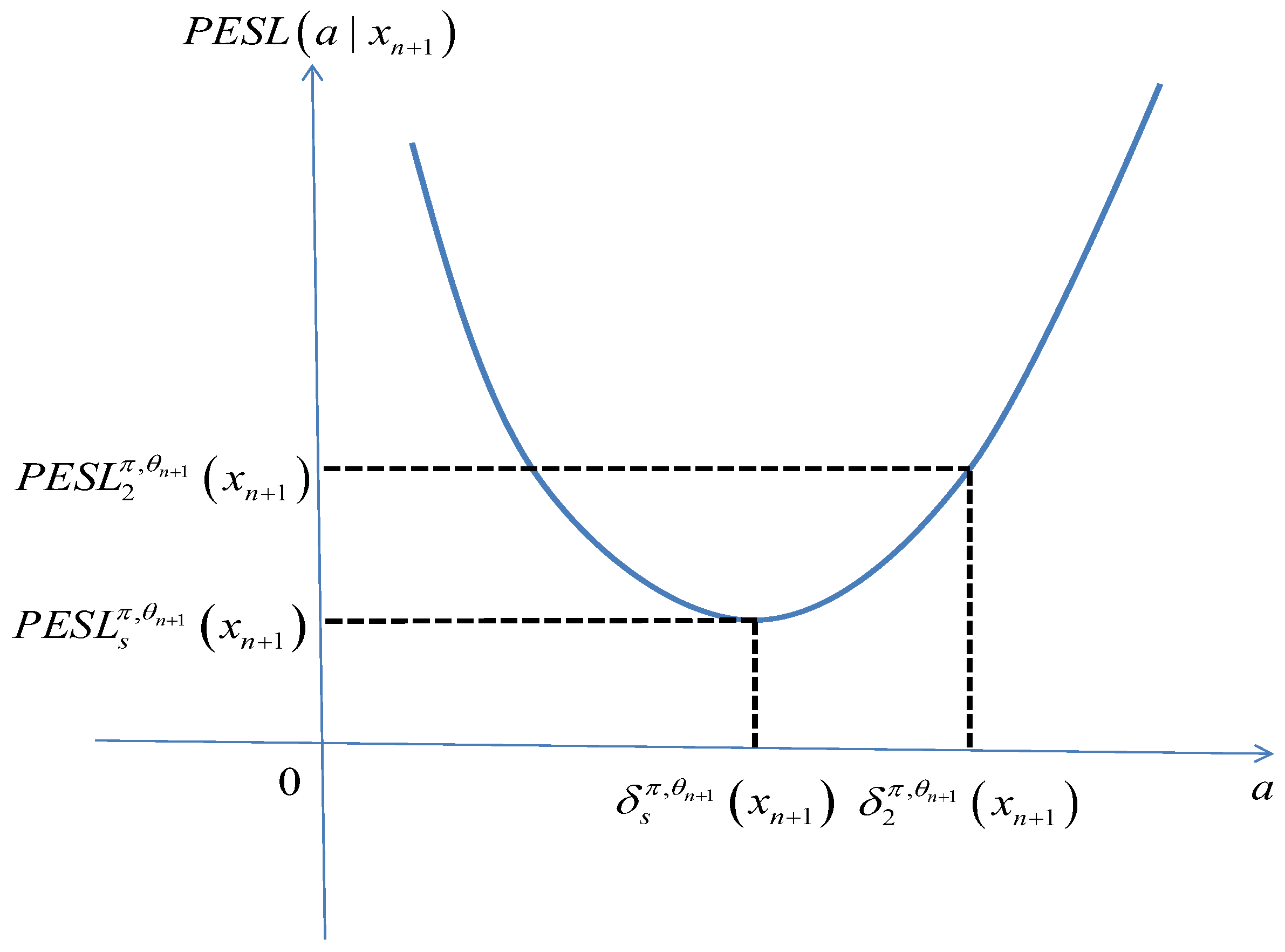
Appendix A.3. The Proof of Theorem 3
The Proof of Theorem 3.
The hyperparameters of Model (2) are , , , and . By Theorem 1, we know that the marginal distribution of X in Model (2) is a non-standardized student-t distribution, that is,
Since there are four hyperparameters, if we want to obtain the estimators of the hyperparameters of Model (2) by the moment method, we need to calculate the first four moments of X at least. By Lemma 4 in [19], we obtain the first six population moments of X as follows. Furthermore, letting the population moments be equal to the sample moments, we obtain
From the first moment of X, we obtain the moment estimator of as
Let
From the second moment of X, we obtain the moment estimator of as
From the third moment of X, we obtain the moment estimator of as
Obviously, the two moment estimators of are not equal. Therefore, we choose one of them as the moment estimator of . For simplicity, we use the moment estimator of calculated from , and ignore the third equation involving . Similarly, the equations involving and both have and . For simplicity, we use the equation involving , and ignore the equation involving . To have four equations, we will use the equation involving . Therefore, the moment equations become
Solving the above moment equations, we obtain
Let
Since and appear together in , we can not directly obtain the estimators of and by the moment method. But we can obtain the estimator of by the moment method. In the following, we are interested in obtaining the moment estimators of , , and . The moment equations involving , , and become
Since there are three equations and only two parameters and , for simplicity, we will only use the first two equations, and ignore the third equation. Solving the above first two equations for and , we obtain the moment estimators of and as
Substituting the expressions of and , and after some algebra, we obtain the expressions of and in terms of as
Therefore, the moment estimators of , , and are given by (A7)–(A9).
Now let us show that the moment estimators are consistent estimators of the hyperparameters. It is easy to show that
for , where means convergence in probability. Hence,
Therefore,
and
The proof of the theorem is complete. □
Appendix A.4. The Proof of Theorem 4
The Proof of Theorem 4.
Now we derive the Maximum Likelihood Estimators (MLEs) of , , and . By Theorem 1, we know that the marginal distribution of X of Model (2) is
for ,, , and . Then the likelihood function of , , and is
Consequently, the log-likelihood function of , , and is
Taking partial derivatives with respect to , , and and setting them to zeros, we obtain
and
where
which can be directly calculated in R software (R x64 4.1.1 and later versions) by digamma(x) [52]. Let
Thus,
After some algebra, the above equations reduce to
In (A10)–(A12), the expressions involving are used for simplifying the R coding.
The MLEs of the hyperparameters , , and are the solutions to the Equations (A10)–(A12). The analytical calculations of the MLEs of , , and by solving the above equations are impossible, and thus we have to resort to numerical solutions. We can exploit Newton’s method to solve the above equations and to obtain the MLEs of , , and . The iterative scheme of Newton’s method is
where is the Jacobian matrix of and . Note that the MLEs of , , and are very sensitive to the initial estimators, and the moment estimators are usually proved to be good initial estimators. The Jacobian matrix of , , and is given by
where
where
Note that
which can be directly calculated in R software by trigamma(x) [52]. In , the expressions involving are used for simplifying the R coding.
Now let us show that the MLEs are consistent estimators of the hyperparameters. From Theorem 10.1.6 in [50], we know that the MLEs are consistent estimators of the hyperparameters under some regularity conditions in Miscellanea 10.6.2 in [50]. The regularity conditions are listed below:
- (C1).
- We observe , where are iid.
- (C2).
- The parameter is identifiable; that is, if , then .
- (C3).
- The densities have common support, and is differentiable in , , and .
- (C4).
- The parameter space contains an open set of which the true parameter value is an interior point.
It remains to show that the marginal distribution satisfies all the regularity conditions. Let be the support set of .
First, (C1) is satisfied, as is a random sample from .
Second, let us show that (C2) is satisfied. The parameter is identifiable
We have
Note that
and thus
Therefore, (A14) is equivalent to
which implies
where is a constant which does not depend on x but may depend on , , , , , and . From (A15), we obtain
and
Substituting (A16) and (A17) into (A15), we obtain
which implies
Substituting (A18) into (A17), we obtain
Therefore,
Consequently, (A13) is correct, and (C2) is satisfied.
Third, (C3) is satisfied, as the densities have common support , and is differentiable in , , and .
Finally, (C4) is satisfied, as the true parameter value
which is an open set.
Therefore, the marginal densities satisfy all the regularity conditions, and the MLEs are consistent estimators of the hyperparameters.
The proof of the theorem is complete. □
Appendix A.5. The Proof of Theorem 5
The Proof of Theorem 5.
The proof of this theorem is simple. By the consistencies of the moment estimators of hyperparameters in Theorem 3, we have
as , for all . Similarly, by the consistencies of the MLEs of hyperparameters in Theorem 4, we obtain
as , for all .
The proof of the theorem is complete. □
References
- Berger, J.O. Statistical Decision Theory and Bayesian Analysis, 2nd ed.; Springer: New York, NY, USA, 1985. [Google Scholar]
- Maritz, J.S.; Lwin, T. Empirical Bayes Methods, 2nd ed.; Chapman & Hall: London, UK, 1989. [Google Scholar]
- Carlin, B.P.; Louis, A. Bayes and Empirical Bayes Methods for Data Analysis, 2nd ed.; Chapman & Hall: London, UK, 2000. [Google Scholar]
- Robbins, H. An empirical Bayes approach to statistics. In Proceedings of the Third Berkeley Symposium on Mathematical Statistics and Probability; University of California Press: Berkeley, CA, USA, 1955; Volume 1. [Google Scholar]
- Robbins, H. The empirical Bayes approach to statistical decision problems. Ann. Math. Stat. 1964, 35, 1–20. [Google Scholar] [CrossRef] [Scilit]
- Robbins, H. Some thoughts on empirical Bayes estimation. Ann. Stat. 1983, 1, 713–723. [Google Scholar] [CrossRef] [Scilit]
- Deely, J.J.; Lindley, D.V. Bayes empirical Bayes. J. Am. Stat. Assoc. 1981, 76, 833–841. [Google Scholar] [CrossRef]
- Morris, C. Parametric empirical Bayes inference: Theory and applications. J. Am. Stat. Assoc. 1983, 78, 47–65. [Google Scholar] [CrossRef]
- Maritz, J.S.; Lwin, T. Assessing the performance of empirical bayes estimators. Ann. Inst. Stat. Math. 1992, 44, 641–657. [Google Scholar] [CrossRef] [Scilit]
- Carlin, B.P.; Louis, A. Empirical Bayes: Past, present and future. J. Am. Stat. Assoc. 2000, 95, 1286–1290. [Google Scholar] [CrossRef]
- Pensky, M. Locally adaptive wavelet empirical Bayes estimation of a location parameter. Ann. Inst. Stat. Math. 2002, 54, 83–99. [Google Scholar] [CrossRef] [Scilit]
- Coram, M.; Tang, H. Improving population-specific allele frequency estimates by adapting supplemental data: An empirical Bayes approach. Ann. Appl. Stat. 2007, 1, 459–479. [Google Scholar] [CrossRef] [Scilit] [PubMed]
- Efron, B. Tweedie’s formula and selection bias. J. Am. Stat. Assoc. 2011, 106, 1602–1614. [Google Scholar] [CrossRef] [Scilit]
- van Houwelingen, H.C. The role of empirical Bayes methodology as a leading principle in modern medical statistics. Biom. J. 2014, 56, 919–932. [Google Scholar] [CrossRef] [Scilit]
- Ghosh, M.; Kubokawa, T.; Kawakubo, Y. Benchmarked empirical Bayes methods in multiplicative area-level models with risk evaluation. Biometrika 2015, 102, 647–659. [Google Scholar] [CrossRef] [Scilit]
- Satagopan, J.M.; Sen, A.; Zhou, Q.; Lan, Q.; Rothman, N.; Langseth, H.; Engel, L.S. Bayes and empirical Bayes methods for reduced rank regression models in matched case-control studies. Biometrics 2016, 72, 584–595. [Google Scholar] [CrossRef] [Scilit] [PubMed]
- Martin, R.; Mess, R.; Walker, S.G. Empirical Bayes posterior concentration in sparse high-dimensional linear models. Bernoulli 2017, 23, 1822–1847. [Google Scholar] [CrossRef] [Scilit]
- Mikulich-Gilbertson, S.K.; Wagner, B.D.; Grunwald, G.K.; Riggs, P.D.; Zerbe, G.O. Using empirical Bayes predictors from generalized linear mixed models to test and visualize associations among longitudinal outcomes. Stat. Methods Med. Res. 2019, 28, 1399–1411. [Google Scholar] [CrossRef] [Scilit] [PubMed]
- Zhang, Y.Y.; Rong, T.Z.; Li, M.M. The empirical Bayes estimators of the mean and variance parameters of the normal distribution with a conjugate normal-inverse-gamma prior by the moment method and the MLE method. Commun. Stat.-Theory Methods 2019, 48, 2286–2304. [Google Scholar] [CrossRef] [Scilit]
- Zhang, Y.Y.; Wang, Z.Y.; Duan, Z.M.; Mi, W. The empirical Bayes estimators of the parameter of the Poisson distribution with a conjugate gamma prior under Stein’s loss function. J. Stat. Comput. Simul. 2019, 89, 3061–3074. [Google Scholar] [CrossRef] [Scilit]
- Sun, J.; Zhang, Y.Y.; Sun, Y. The empirical Bayes estimators of the rate parameter of the inverse gamma distribution with a conjugate inverse gamma prior under Stein’s loss function. J. Stat. Comput. Simul. 2021, 91, 1504–1523. [Google Scholar] [CrossRef] [Scilit]
- Zhou, M.Q.; Zhang, Y.Y.; Sun, Y.; Sun, J.; Rong, T.Z.; Li, M.M. The empirical Bayes estimators of the probability parameter of the beta-negative binomial model under Zhang’s loss function. Chin. J. Appl. Probab. Stat. 2021, 37, 478–494. [Google Scholar]
- Sun, Y.; Zhang, Y.Y.; Sun, J. The empirical Bayes estimators of the parameter of the uniform distribution with an inverse gamma prior under Stein’s loss function. Commun. Stat.-Simul. Comput. 2024, 53, 3027–3045. [Google Scholar] [CrossRef] [Scilit]
- Zhang, Y.Y.; Zhang, Y.Y.; Wang, Z.Y.; Sun, Y.; Sun, J. The empirical Bayes estimators of the variance parameter of the normal distribution with a conjugate inverse gamma prior under Stein’s loss function. Commun. Stat.-Theory Methods 2024, 53, 170–200. [Google Scholar] [CrossRef] [Scilit]
- Mao, S.S.; Tang, Y.C. Bayesian Statistics, 2nd ed.; China Statistics Press: Beijing, China, 2012.
- Chen, M.H. Bayesian Statistics Lecture; Statistics Graduate Summer School, School of Mathematics and Statistics, Northeast Normal University: Changchun, China, 2014. [Google Scholar]
- James, W.; Stein, C. Estimation with Quadratic Loss. In Proceedings of the Fourth Berkeley Symposium on Mathematical Statistics and Probability; University of California: Berkeley, CA, USA, 1961; Volume 1, pp. 361–380. [Google Scholar]
- Zhang, Y.Y. The Bayes rule of the variance parameter of the hierarchical normal and inverse gamma model under Stein’s loss. Commun. Stat.-Theory Methods 2017, 46, 7125–7133. [Google Scholar] [CrossRef] [Scilit]
- Xie, Y.H.; Song, W.H.; Zhou, M.Q.; Zhang, Y.Y. The Bayes posterior estimator of the variance parameter of the normal distribution with a normal-inverse-gamma prior under Stein’s loss. Chin. J. Appl. Probab. Stat. 2018, 34, 551–564. [Google Scholar]
- Zhang, Y.Y.; Xie, Y.H.; Song, W.H.; Zhou, M.Q. Three strings of inequalities among six Bayes estimators. Commun. Stat.-Theory Methods 2018, 47, 1953–1961. [Google Scholar] [CrossRef] [Scilit]
- Good, I.J. Turing’s anticipation of empirical Bayes in connection with the cryptanalysis of the naval enigma. J. Stat. Comput. Simul. 2000, 66, 101–111. [Google Scholar] [CrossRef] [Scilit]
- Noma, H.; Matsui, S. Empirical Bayes ranking and selection methods via semiparametric hierarchical mixture models in microarray studies. Stat. Med. 2013, 32, 1904–1916. [Google Scholar] [CrossRef] [Scilit]
- Pan, W.; Jeong, K.S.; Xie, Y.; Khodursky, A. A nonparametric empirical Bayes approach to joint modeling of multiple sources of genomic data. Stat. Sin. 2008, 18, 709–729. [Google Scholar]
- Zhang, Q.; Xu, Z.; Lai, Y. An empirical Bayes approach for the identification of long-range chromosomal interaction from Hi-C data. Stat. Appl. Genet. Mol. Biol. 2021, 20, 1–15. [Google Scholar] [CrossRef] [Scilit]
- Soloff, J.A.; Guntuboyina, A.; Sen, B. Multivariate, heteroscedastic empirical Bayes via nonparametric maximum likelihood. J. R. Stat. Soc. Ser. B-Stat. Methodol. 2024, 87, 1–32. [Google Scholar] [CrossRef] [Scilit]
- Zhang, Y.Y.; Rong, T.Z.; Li, M.M. The Bayes estimator of the positive restricted parameter under the power-power loss with an application. Chin. J. Appl. Probab. Stat. 2023, 39, 159–177. [Google Scholar]
- Adler, D.; Murdoch, D. rgl: 3D Visualization Using OpenGL, R Package Version 0.98.1. 2017.
- Conover, W.J. Practical Nonparametric Statistics. New York: John Wiley & Sons. Pages 295–301 (one-sample Kolmogorov test), 309–314 (two-sample Smirnov test). In Proceedings of the Practical Nonparametric Statistics; Wiley: New York, NY, USA, 1971. [Google Scholar]
- Durbin, J. Distribution Theory for Tests Based on the Sample Distribution Function; SIAM: Philadelphia, PA, USA, 1973. [Google Scholar]
- Marsaglia, G.; Tsang, W.W.; Wang, J.B. Evaluating Kolmogorov’s distribution. J. Stat. Softw. 2003, 8, 1–4. [Google Scholar] [CrossRef] [Scilit]
- Aldirawi, H.; Yang, J.; Metwally, A.A. Identifying appropriate probabilistic models for sparse discrete omics data. In Proceedings of the IEEE EMBS International Conference on Biomedical and Health Informatics (BHI), Chicago, IL, USA, 19–22 May 2019. [Google Scholar]
- Dimitrova, D.S.; Kaishev, V.K.; Tan, S. Computing the Kolmogorov-Smirnov distribution when the underlying cdf is purely discrete, mixed or continuous. J. Stat. Softw. 2020, 95, 1–42. [Google Scholar] [CrossRef] [Scilit]
- Santitissadeekorn, N.; Lloyd, D.J.B.; Short, M.B.; Delahaies, S. Approximate filtering of conditional intensity process for Poisson count data: Application to urban crime. Comput. Stat. Data Anal. 2020, 144, 106850. [Google Scholar] [CrossRef] [Scilit]
- Anderson, T.W.; Darling, D.A. A test of goodness of fit. J. Am. Stat. Assoc. 1954, 49, 765–769. [Google Scholar] [CrossRef]
- Braun, H. A simple method for testing goodness-of-fit in the presence of nuisance parameters. J. R. Stat. Soc. Ser. B-Stat. Methodol. 1980, 42, 53–63. [Google Scholar] [CrossRef] [Scilit]
- Marsaglia, G.; Marsaglia, J. Evaluating the Anderson-Darling distribution. J. Stat. Softw. 2004, 9, 1–5. [Google Scholar] [CrossRef] [Scilit]
- Csorgo, S.; Faraway, J.J. The exact and asymptotic distributions of Cramer-von Mises statistics. J. R. Stat. Soc. Ser. B-Stat. Methodol. 1996, 58, 221–234. [Google Scholar] [CrossRef] [Scilit]
- Berger, J.O. The case for objective Bayesian analysis. Bayesian Anal. 2006, 1, 385–402. [Google Scholar] [CrossRef] [Scilit]
- Berger, J.O.; Bernardo, J.M.; Sun, D.C. Overall objective priors. Bayesian Anal. 2015, 10, 189–221. [Google Scholar] [CrossRef] [Scilit]
- Casella, G.; Berger, R.L. Statistical Inference, 2nd ed.; Duxbury: Pacific Grove, CA, USA, 2002. [Google Scholar]
- Robert, C.P. The Bayesian Choice: From Decision-Theoretic Motivations to Computational Implementation, 2nd ed.; Springer: New York, NY, USA, 2007. [Google Scholar]
- R Core Team. R: A Language and Environment for Statistical Computing; R Foundation for Statistical Computing: Vienna, Austria, 2026. [Google Scholar]
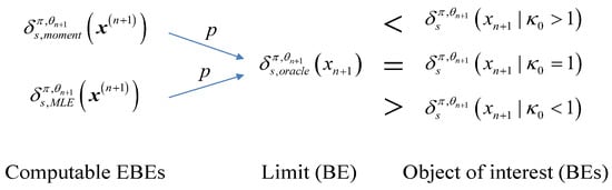
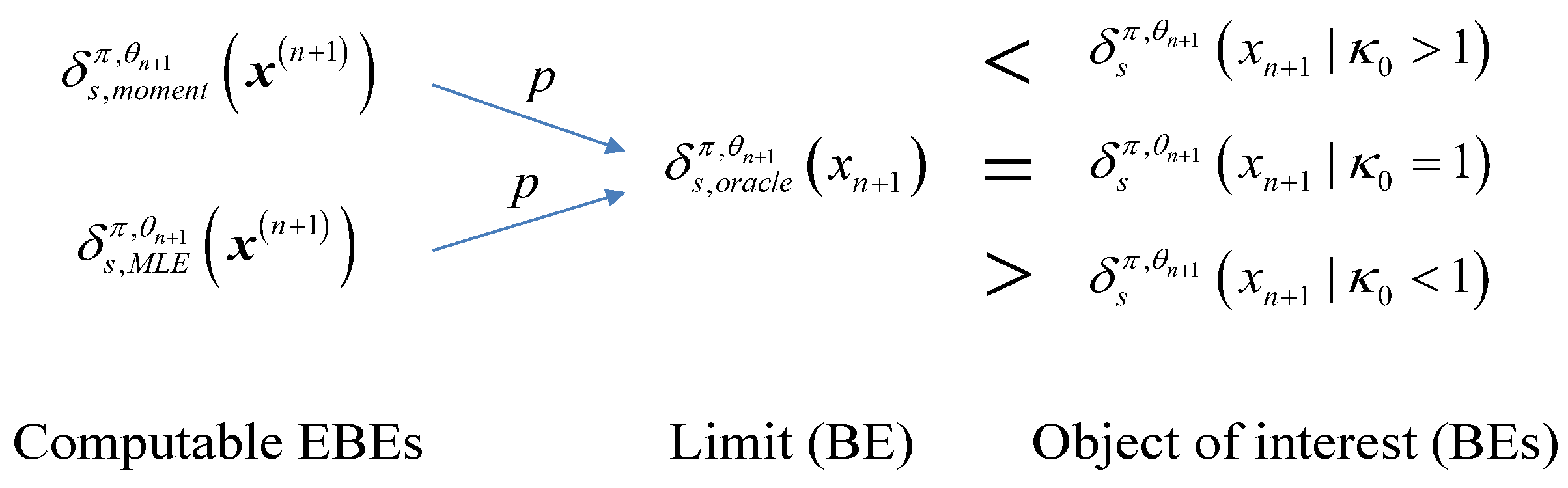
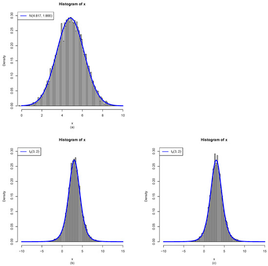
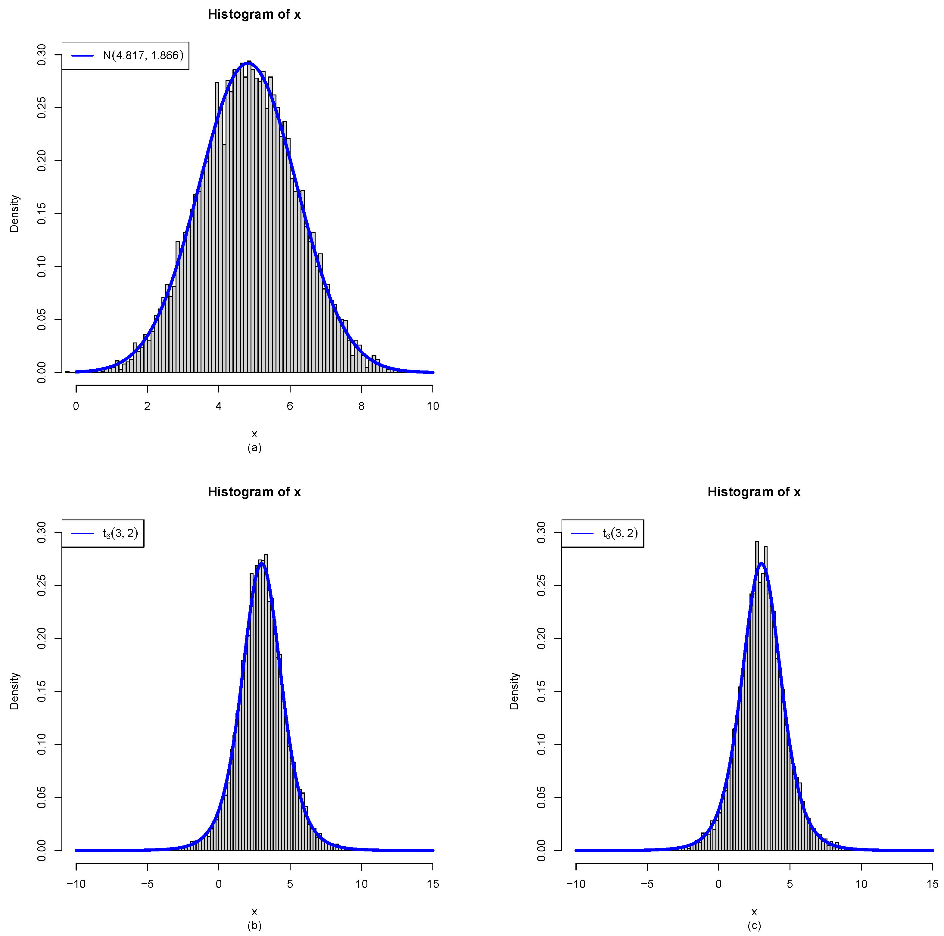
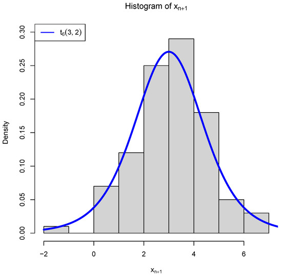
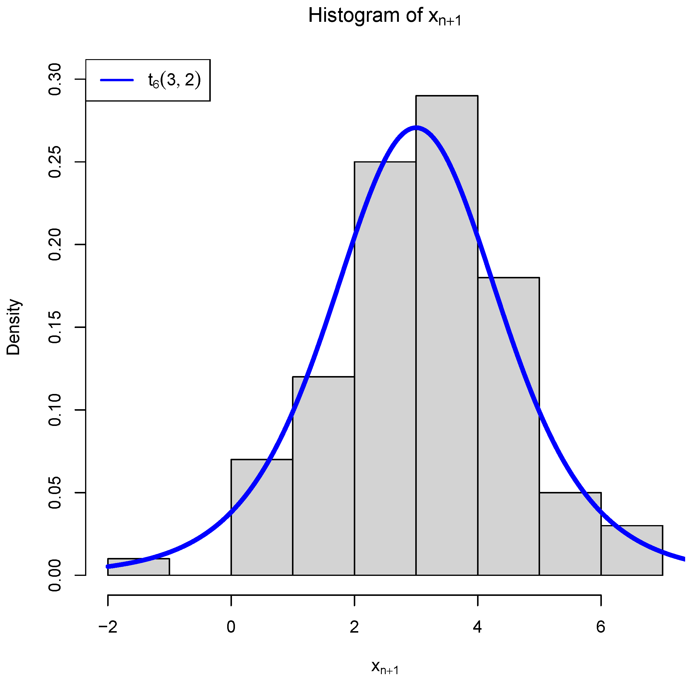
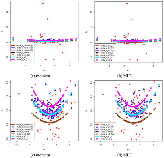
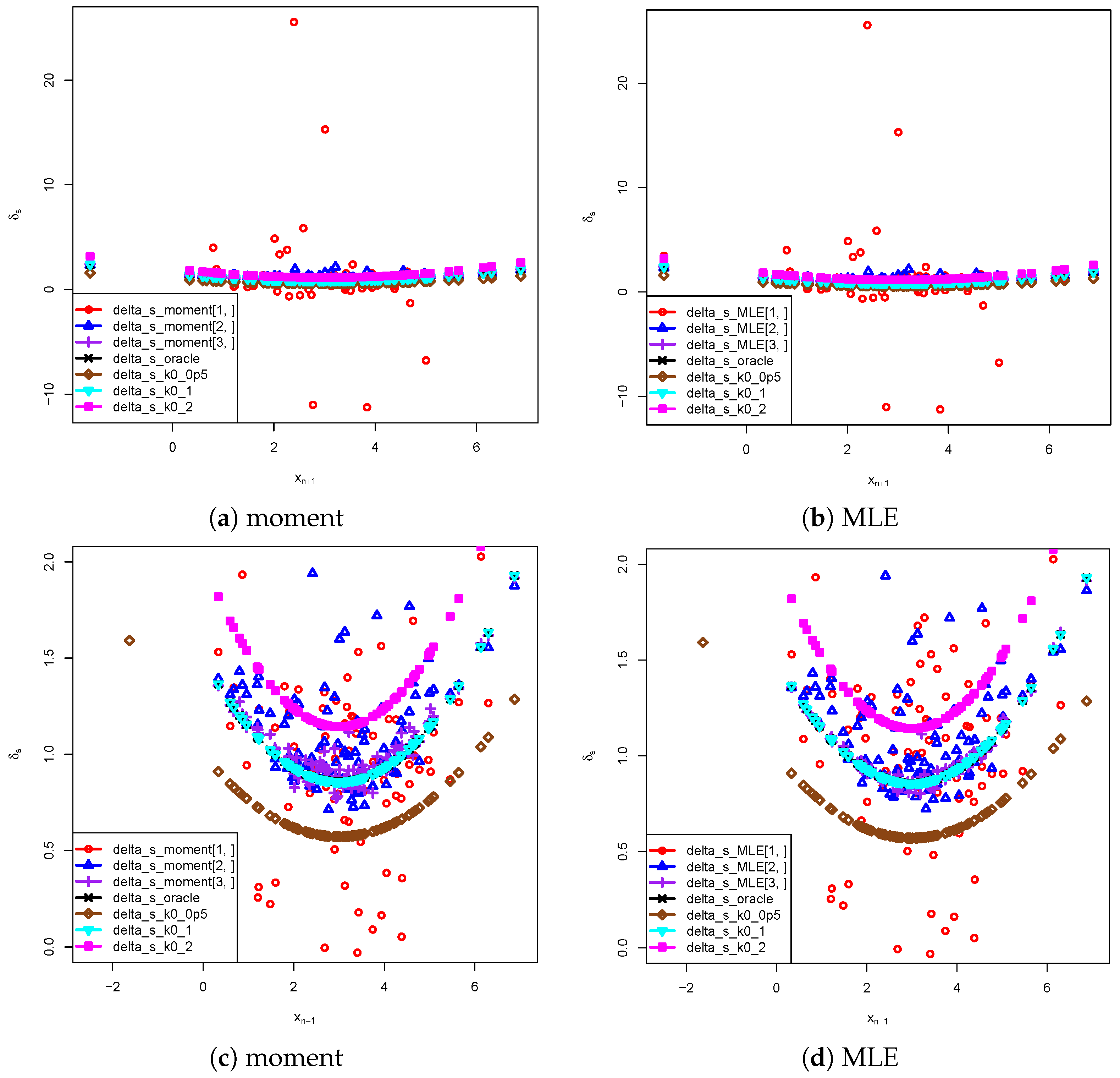
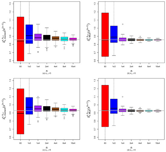
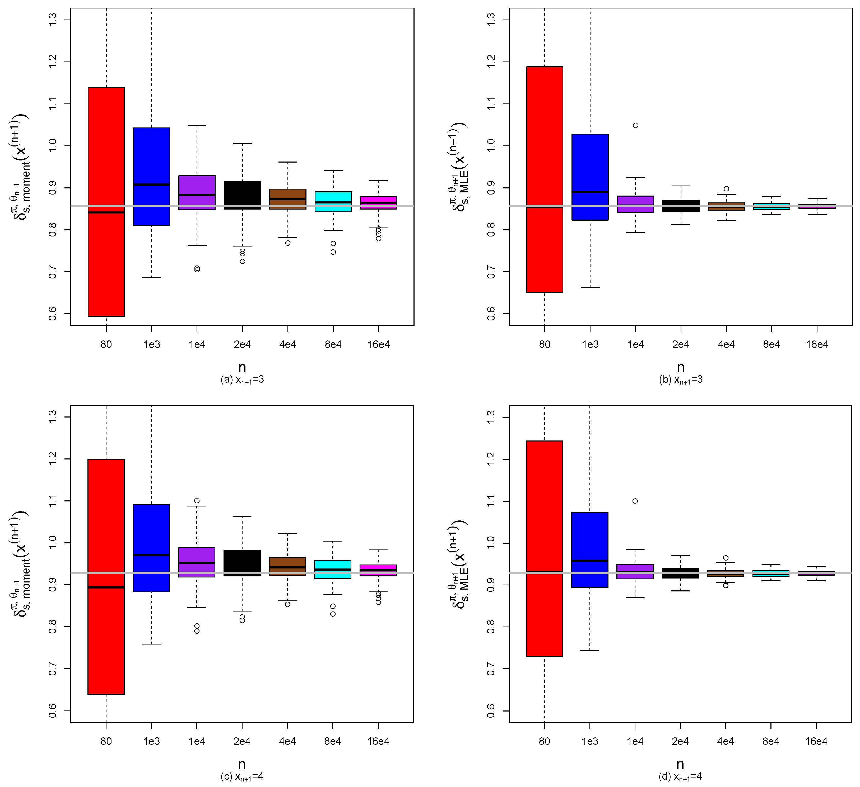
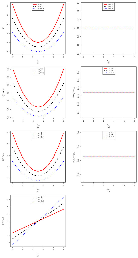
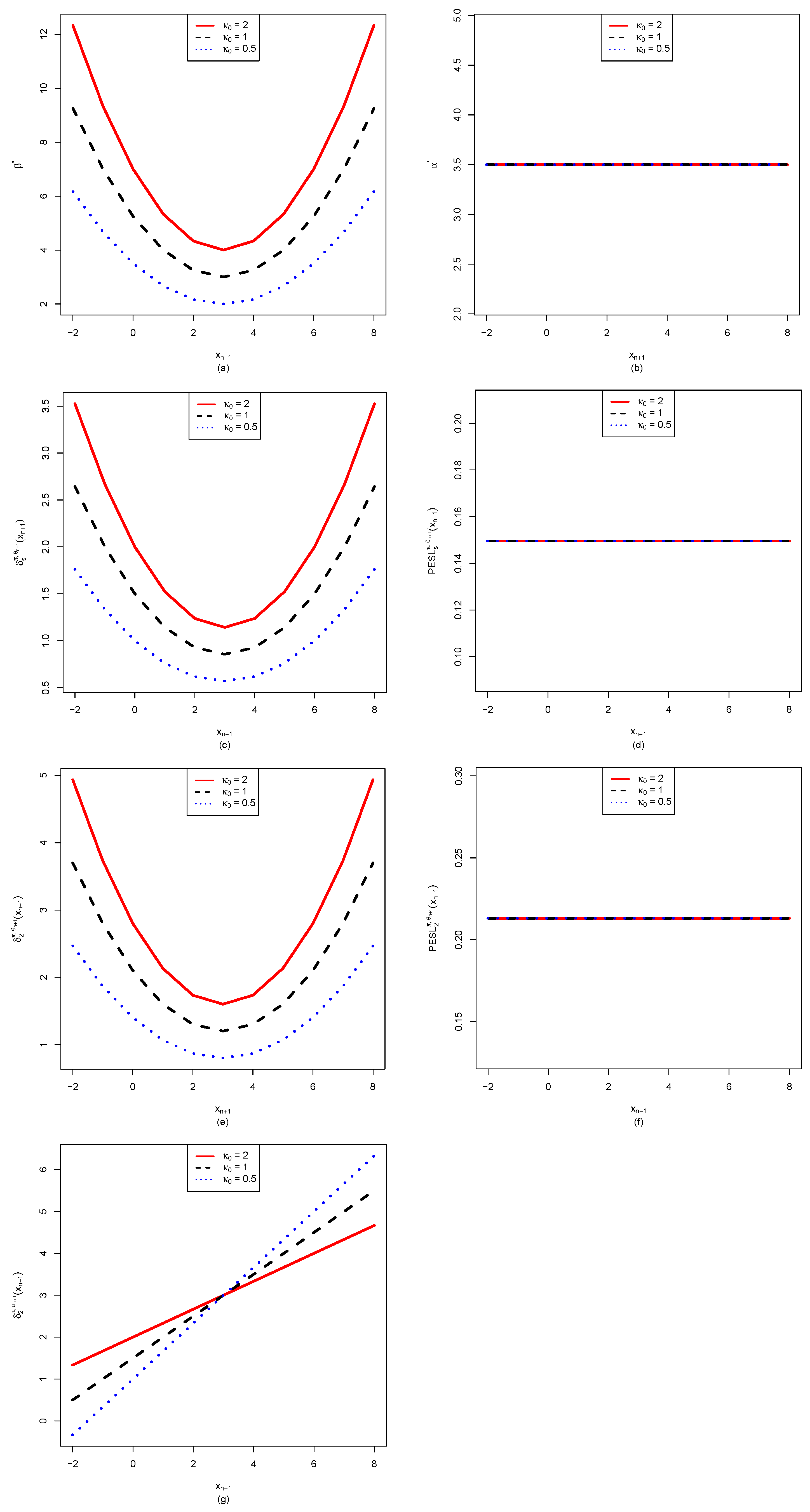
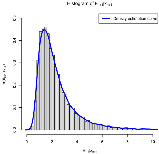
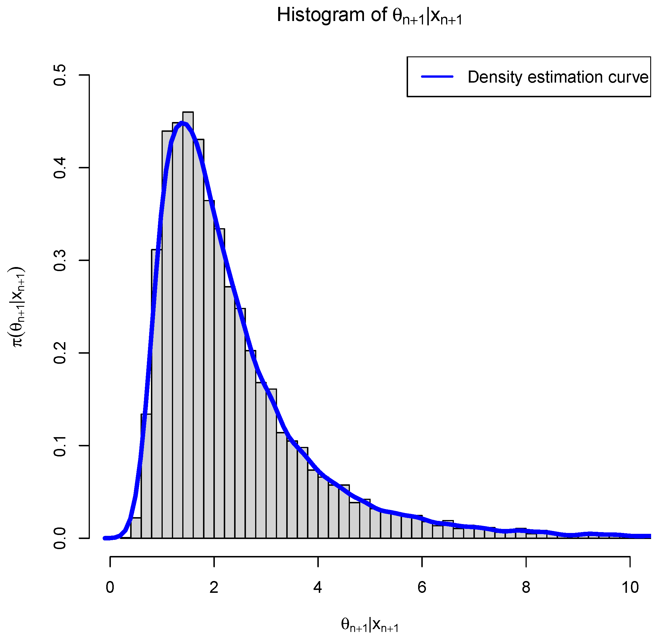
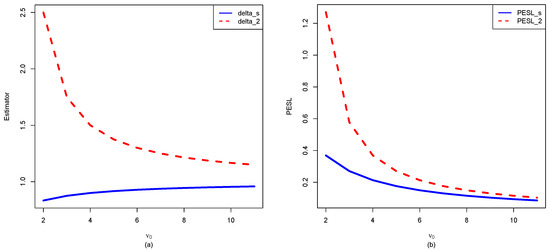
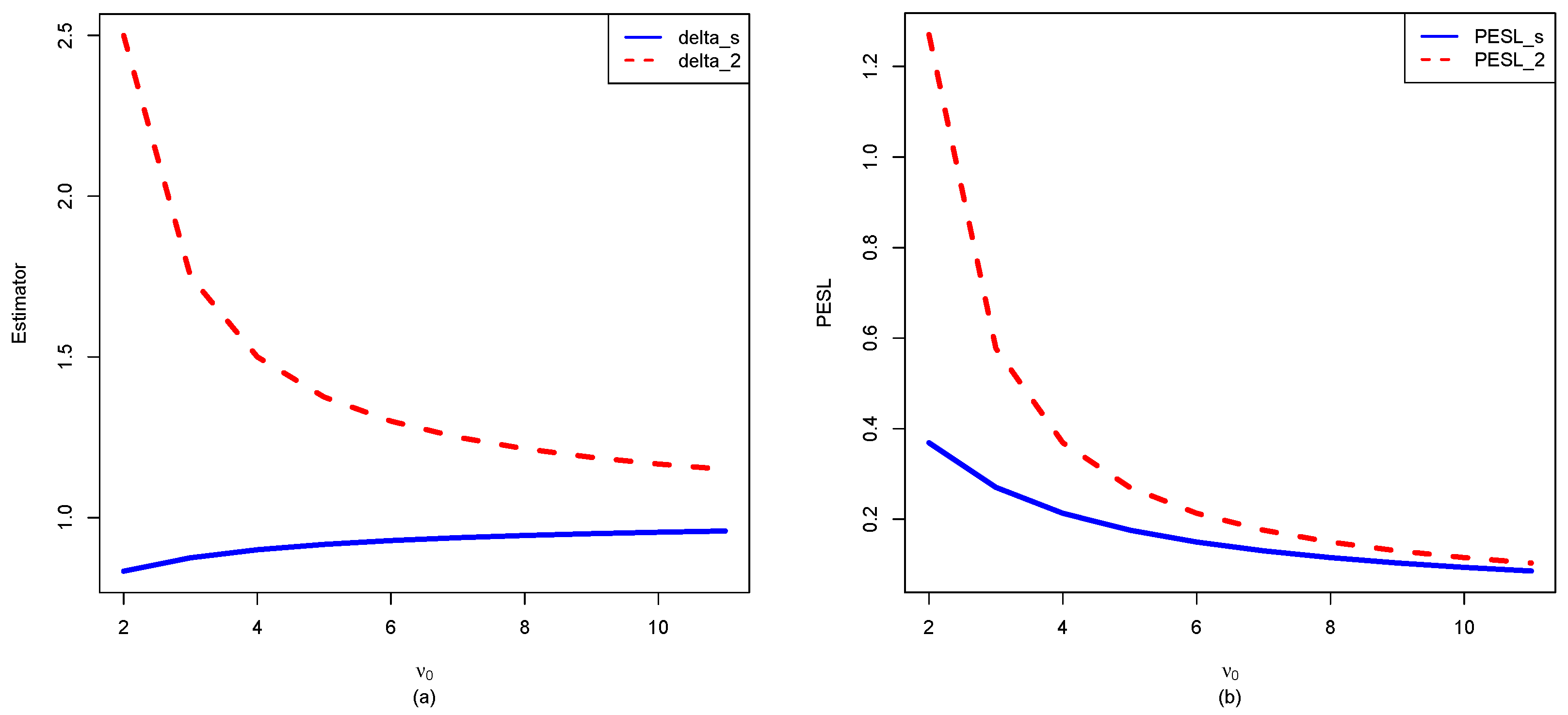
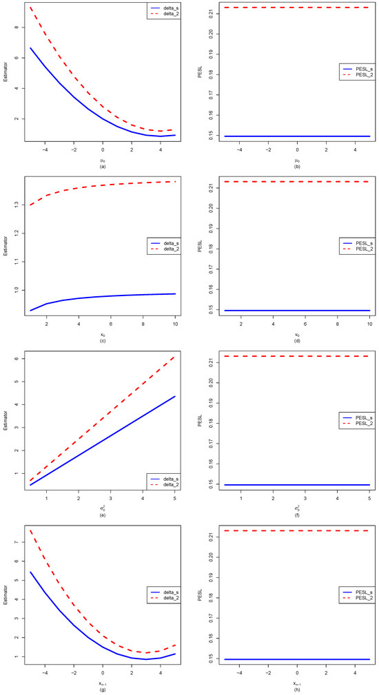
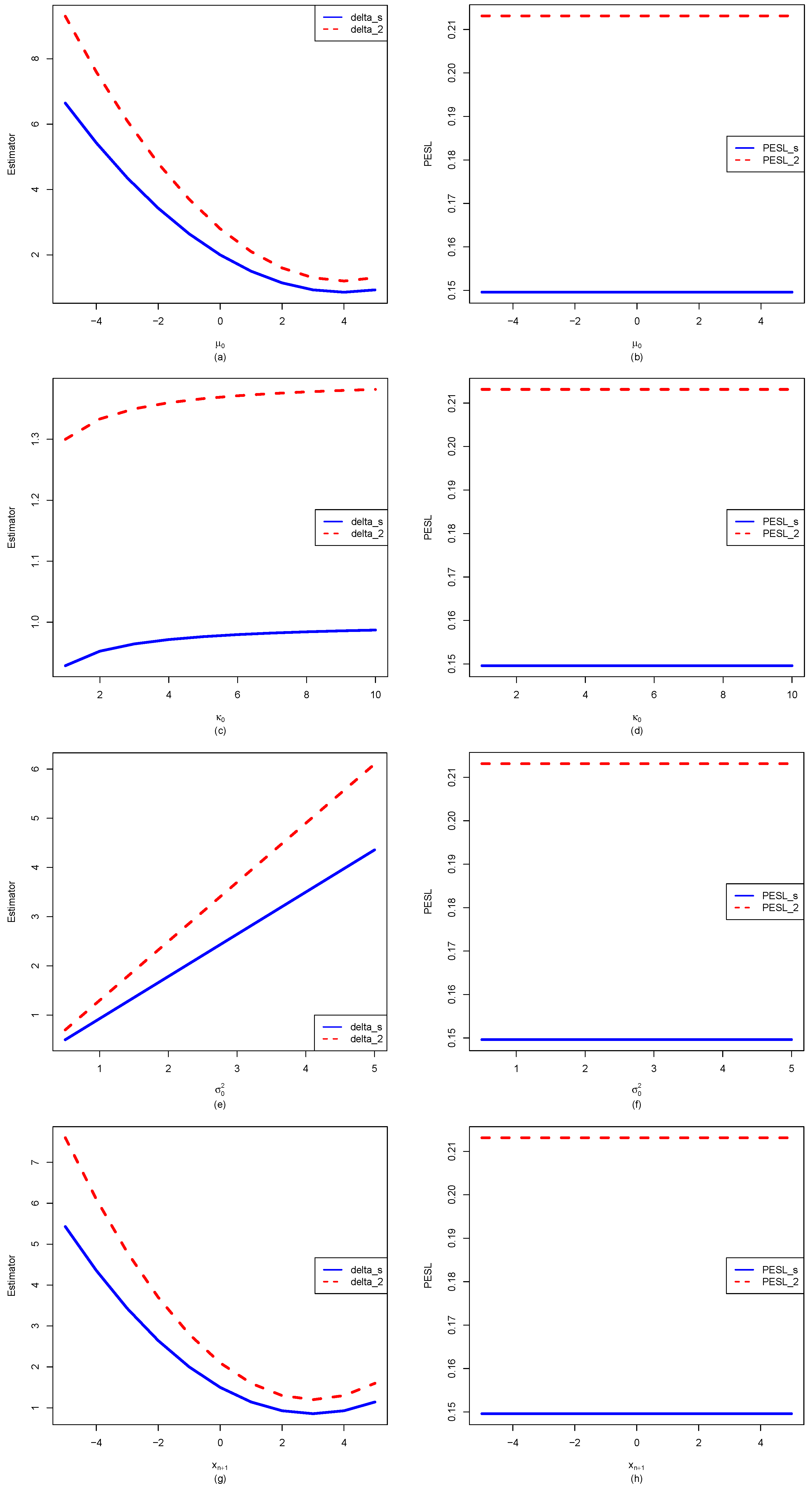
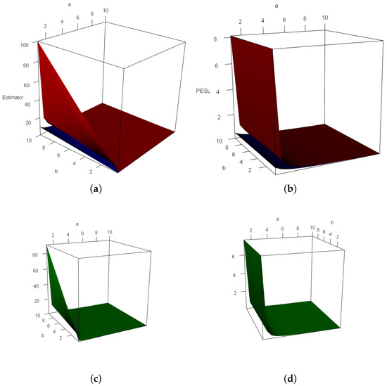
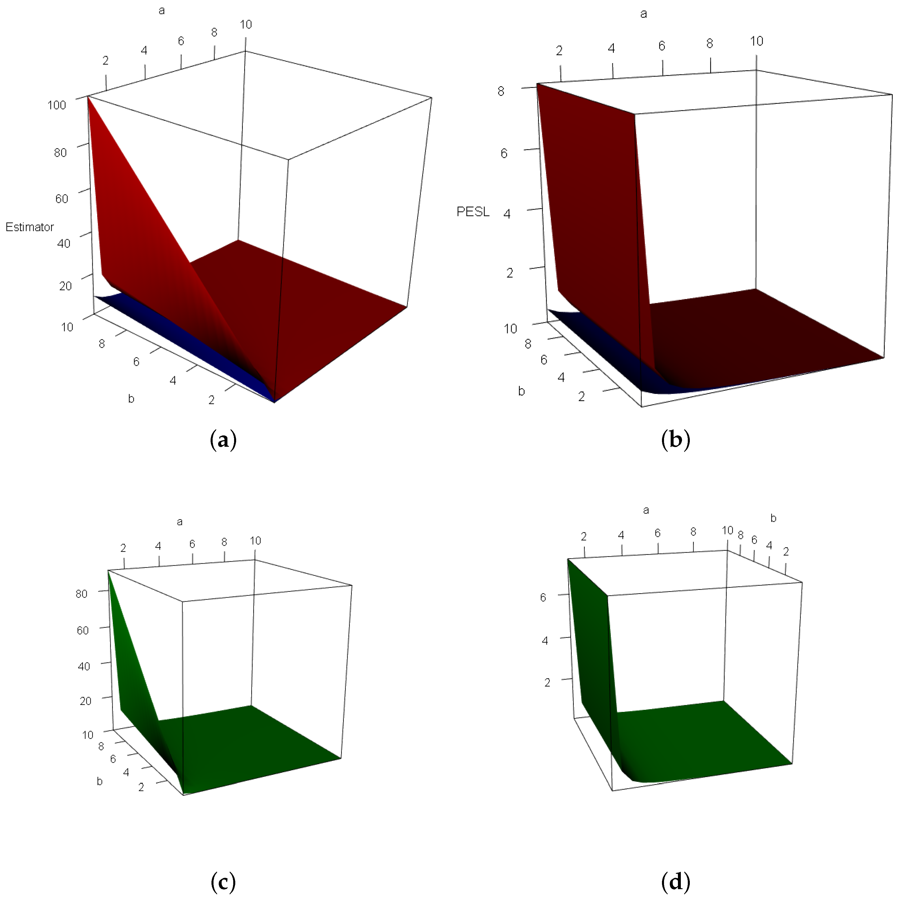
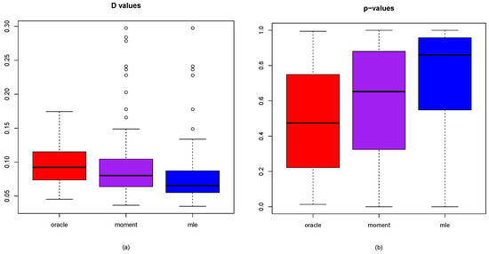
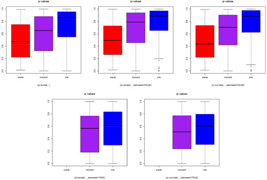
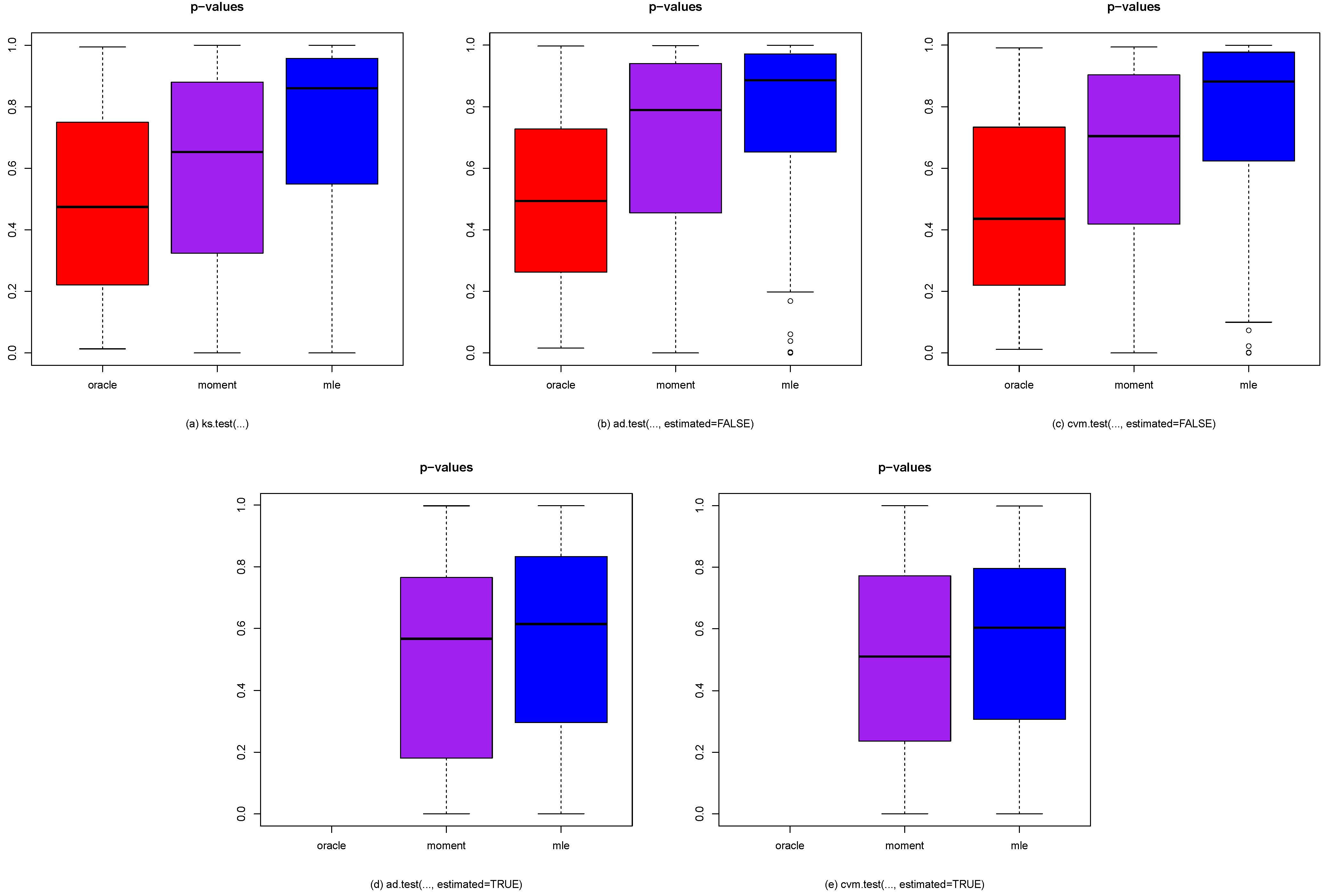
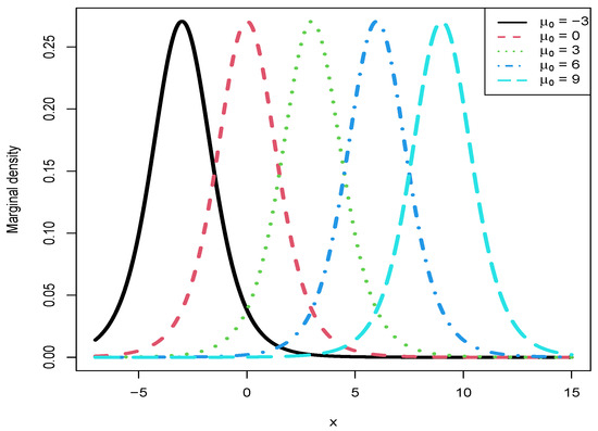
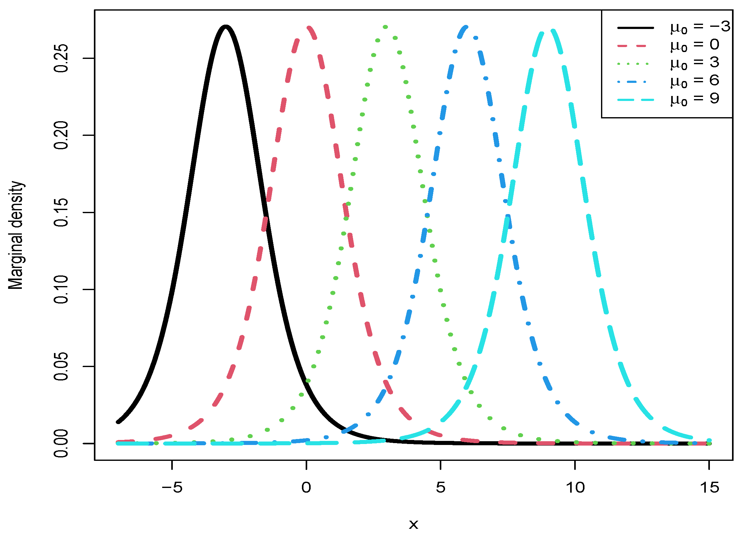
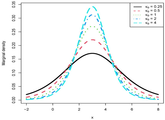
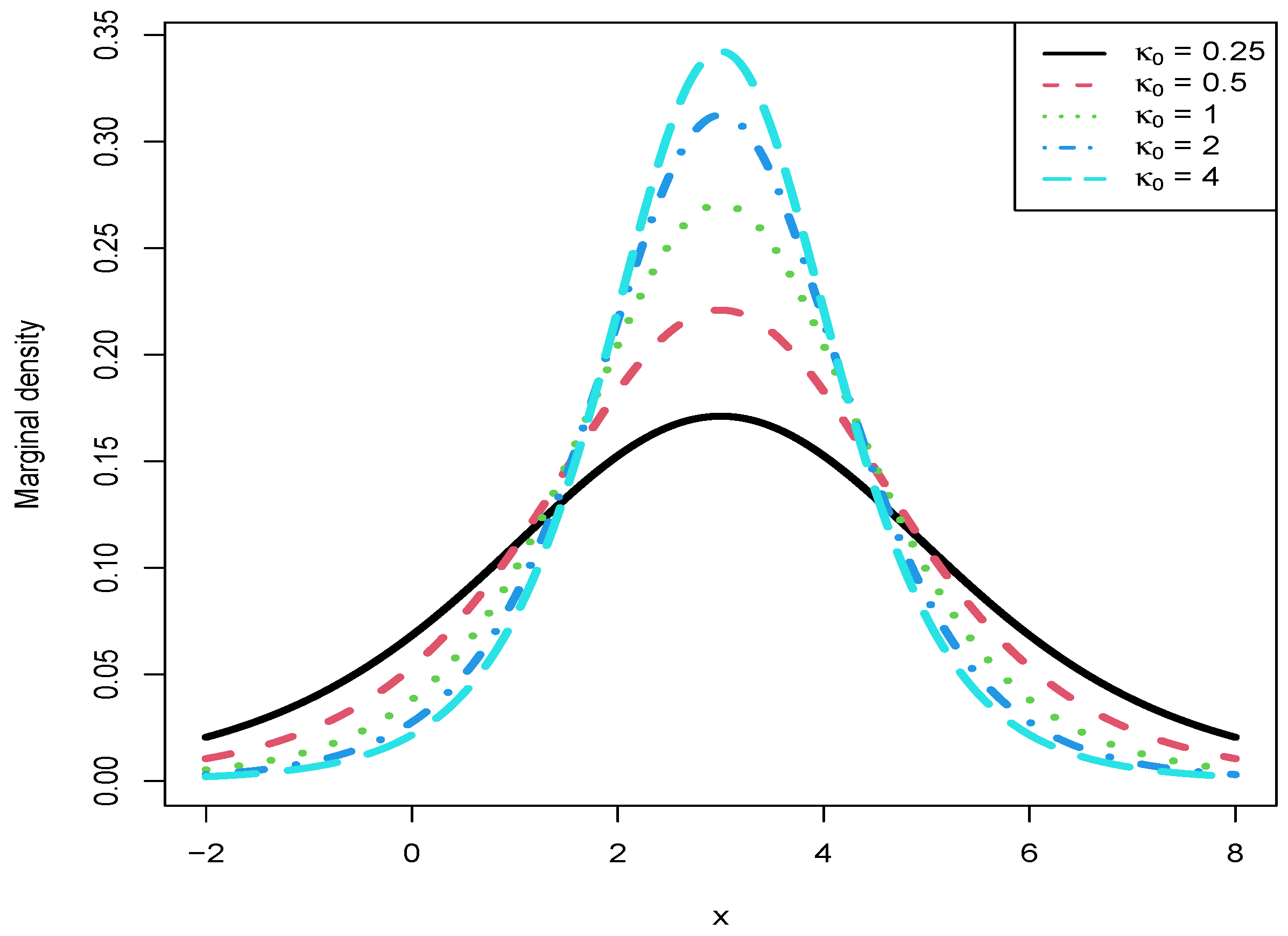
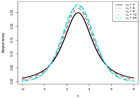
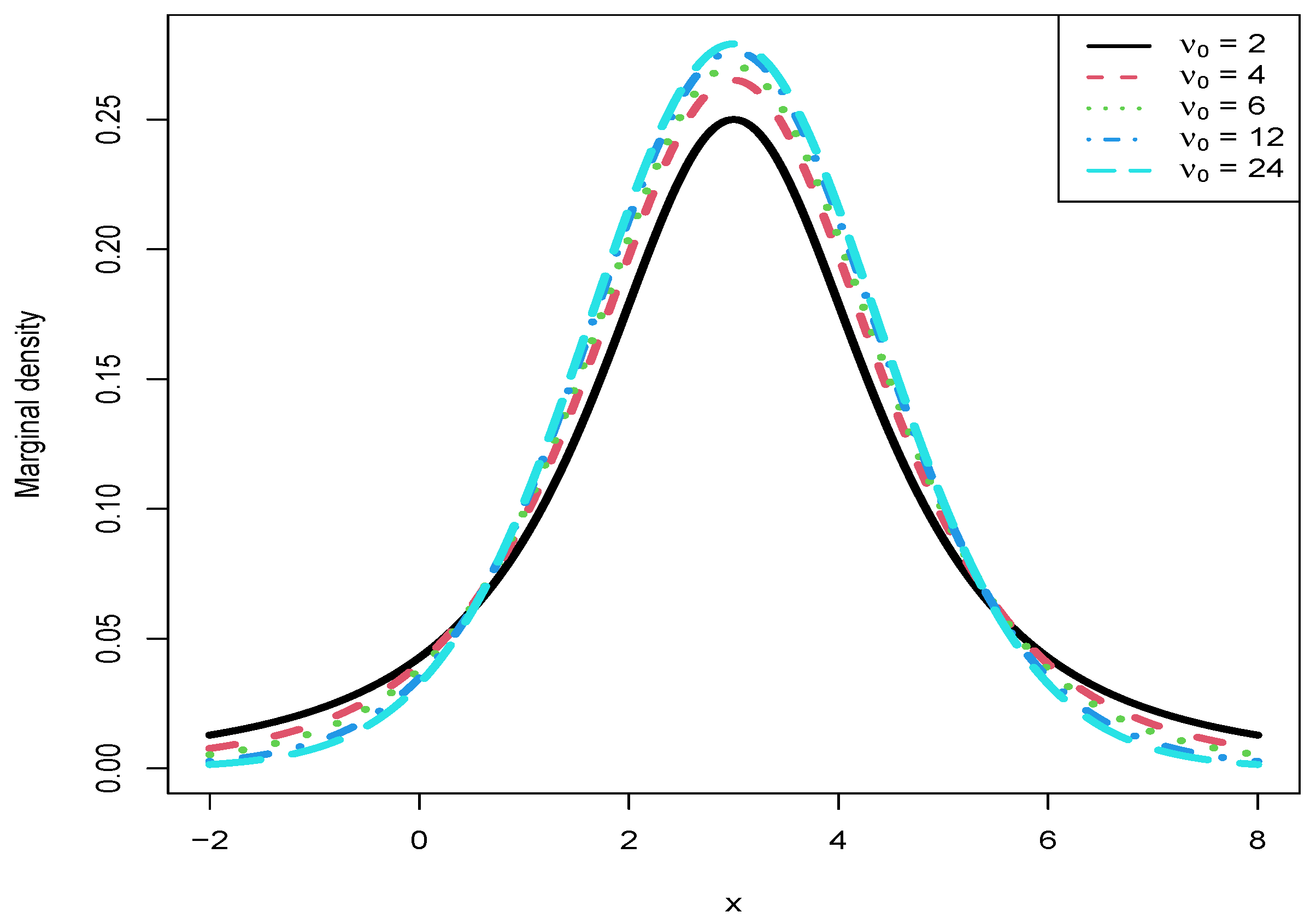
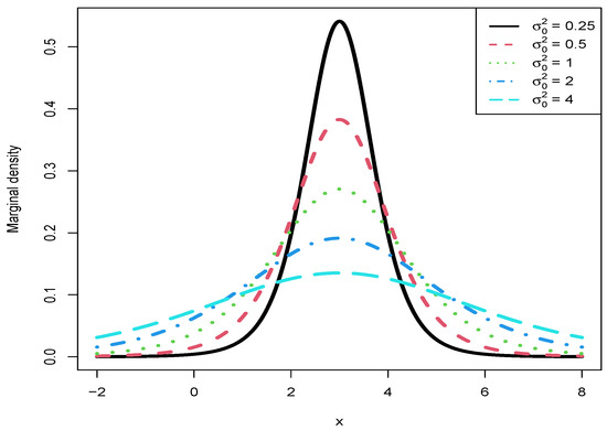
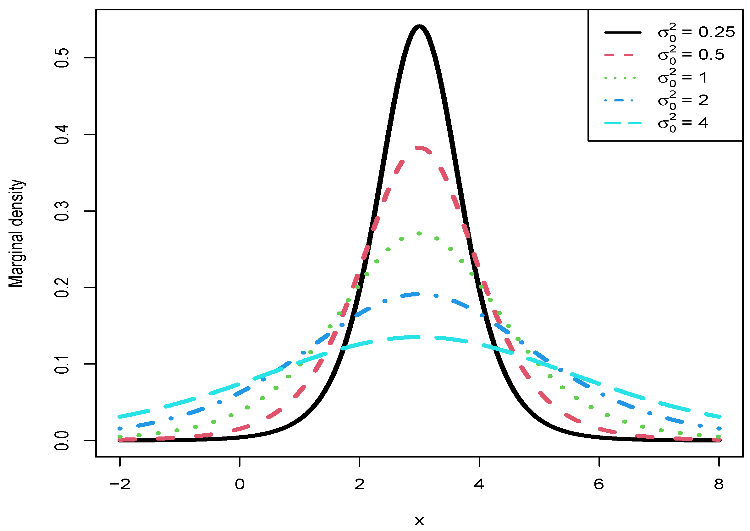
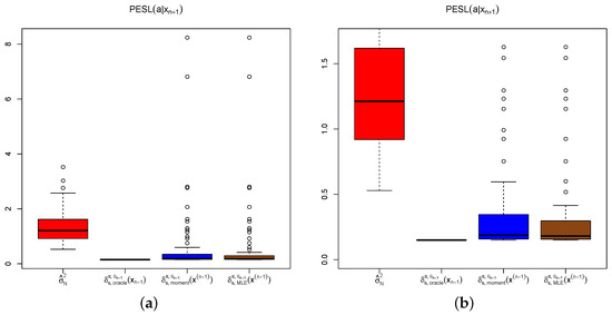
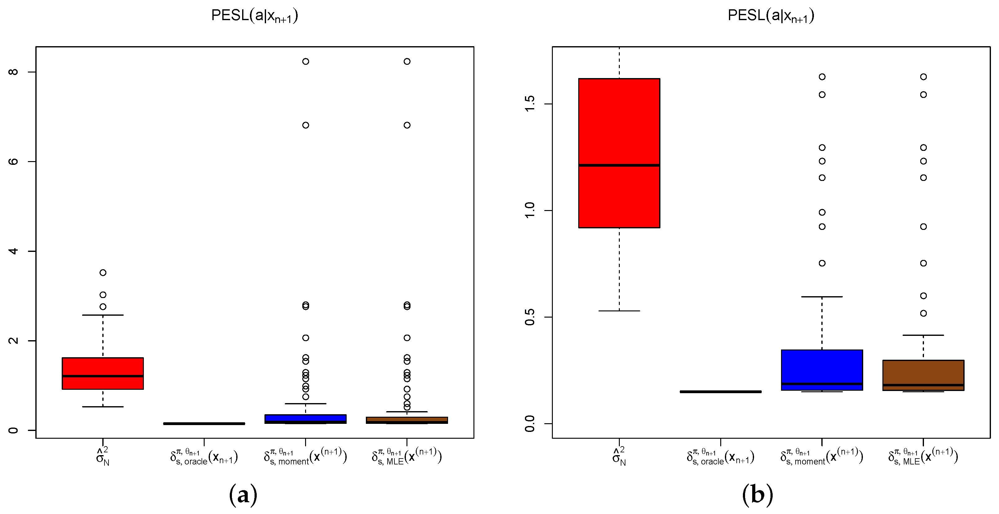
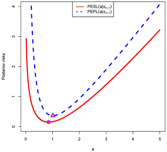
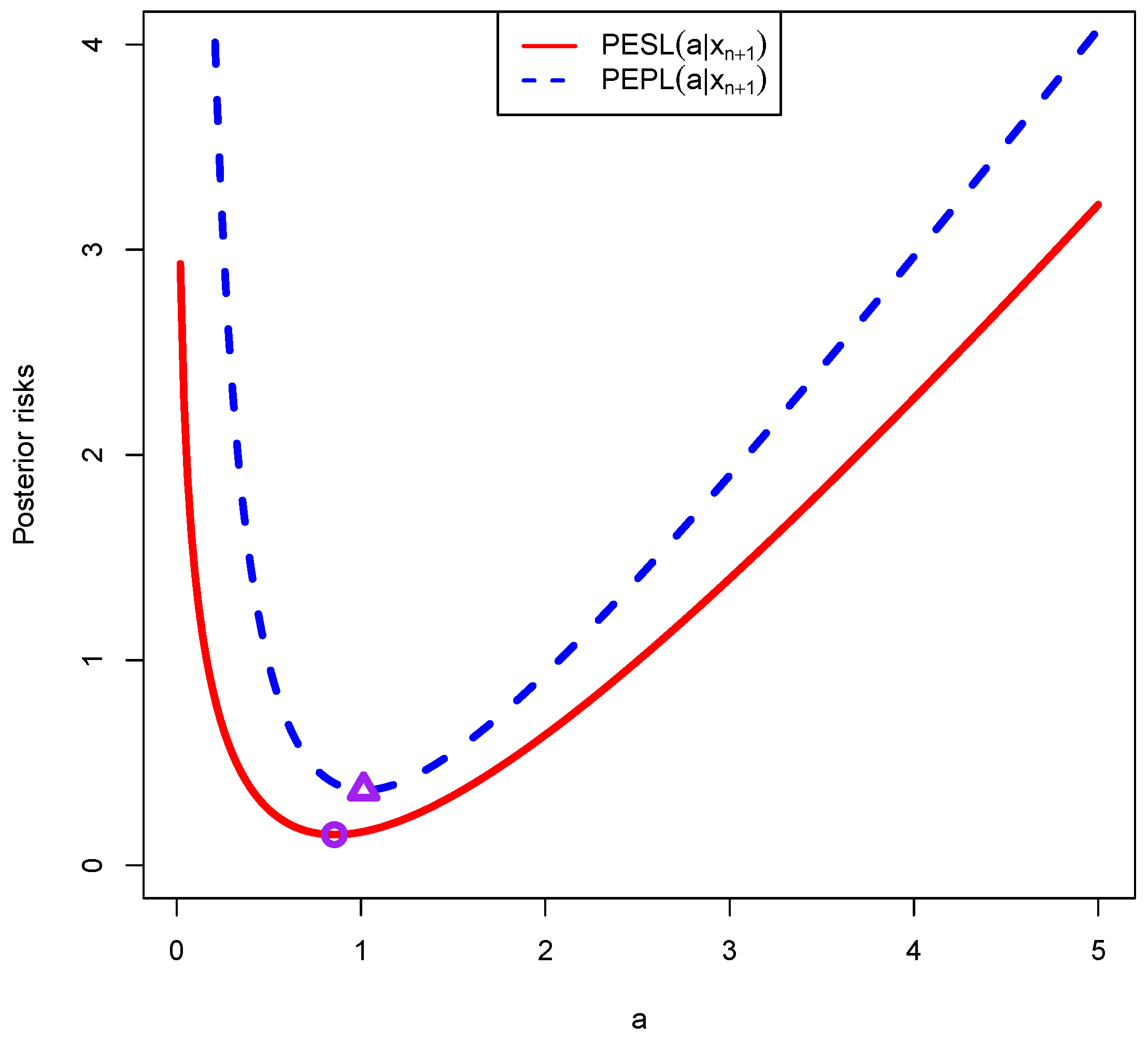
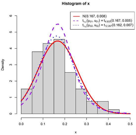
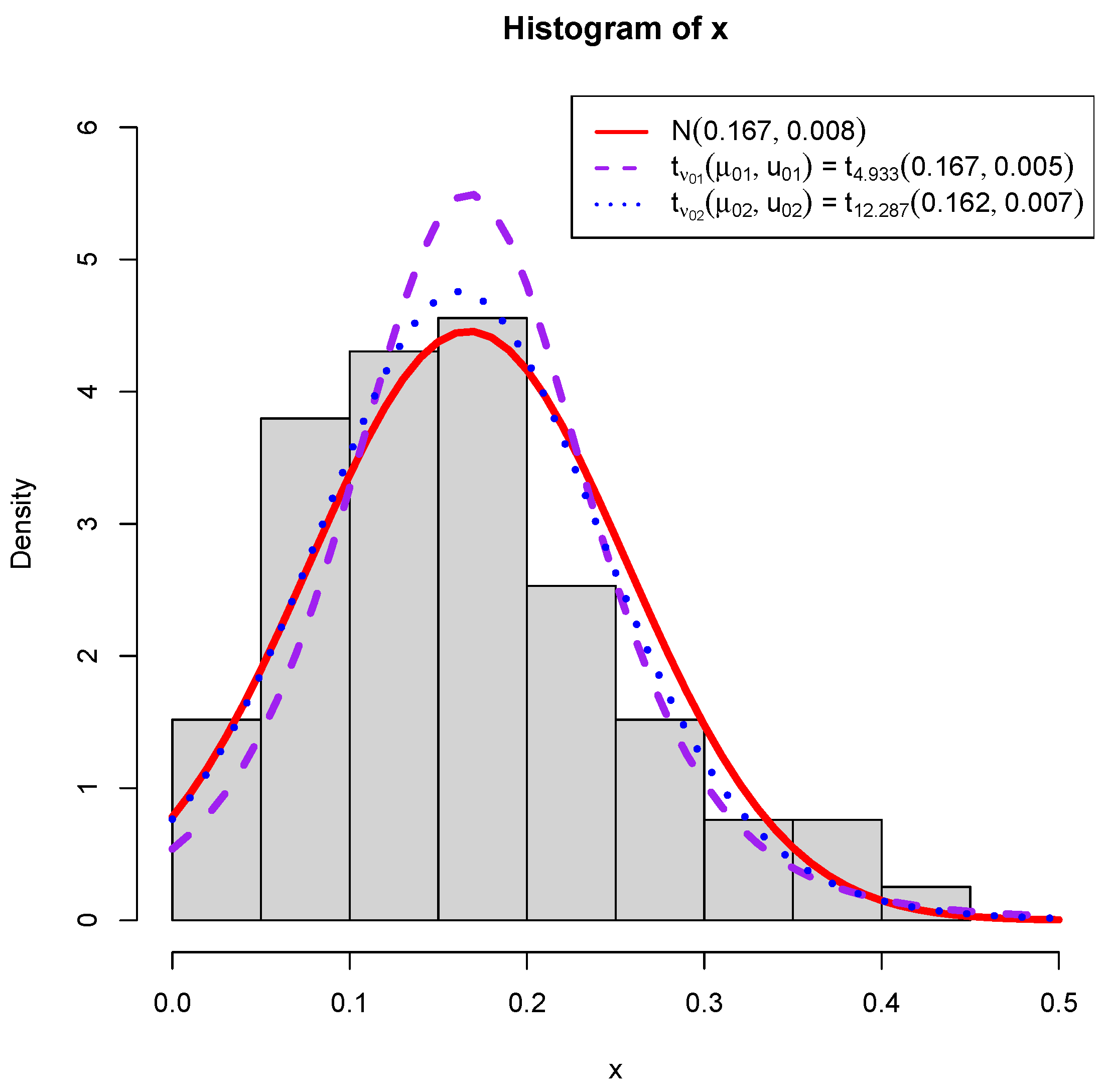

Disclaimer/Publisher’s Note: The statements, opinions and data contained in all publications are solely those of the individual author(s) and contributor(s) and not of MDPI and/or the editor(s). MDPI and/or the editor(s) disclaim responsibility for any injury to people or property resulting from any ideas, methods, instructions or products referred to in the content. |
© 2026 by the author. Licensee MDPI, Basel, Switzerland. This article is an open access article distributed under the terms and conditions of the Creative Commons Attribution (CC BY) license.