An Algorithm for Computing the Singularities of the Plane Model of X₀(N)

Abstract

Let ${\mathrm{\Phi }}_N(X,Y)$ be the N-th classical modular polynomial and let $Z_0\left(N\right)=\{(X,Y)\in {\mathbb{C}}^2\mid {\mathrm{\Phi }}_N(X,Y)=0\}$ be the plane model of the modular curve $X_0\left(N\right)$. We present an explicit procedure that, for a prime ℓ, enumerates all non-cuspidal singular points of $Z_0(\ell )$ over $\mathbb{C}$ and outputs the corresponding pairs of distinct points on $X_0(\ell )$ mapping to each node. The method relies on the arithmetic (CM) classification of self-intersections of the map $X_0(\ell )\to Z_0(\ell )$ and on effective computations of proper ideal classes in imaginary quadratic orders. We also provide a complete and self-contained exposition of Kara’s proof of the automorphism-group equality $Aut\left(E\right)=Aut\left(E^{\prime }\right)$ in the self-intersection setting, making explicit where Kolyvagin’s conductor lemma is used essentially. Finally, we discuss termination, correctness, and practical complexity issues, and we report computational evidence for larger primes using a parallel implementation; in particular, for $\ell =389$, we obtained $151,288$ output pairs in $151,017$ seconds on a 56-core machine.

1. Introduction

Let $j\left(\tau \right)=j\left(L_{\tau }\right)$ denote the classical j-invariant of the elliptic curve $\mathbb{C}/L_{\tau }$ with $L_{\tau }=\mathbb{Z}+\mathbb{Z}\tau$ for $\tau \in \mathcal{H}$. We will repeatedly use the standard equivalences (see [1]): for ${\tau }_1,{\tau }_2\in \mathcal{H}$, one has $j\left({\tau }_1\right)=j\left({\tau }_2\right)$ if and only if ${\tau }_2=\gamma \left({\tau }_1\right)$ for some $\gamma \in S{L}_2\left(\mathbb{Z}\right)$, and for lattices $L_1,L_2\subset \mathbb{C}$, one has $j\left(L_1\right)=j\left(L_2\right)$ if and only if $L_2=\lambda L_1$ for some $\lambda \in {\mathbb{C}}^{\times }$; equivalently, $\mathbb{C}/L_1\cong \mathbb{C}/L_2$. Moreover, for an integer $N\ge 2$, the N-th modular polynomial ${\mathrm{\Phi }}_N(X,Y)$ satisfies ${\mathrm{\Phi }}_N(j\left(E_1\right),j\left(E_2\right))=0$ if and only if $E_1$ and $E_2$ are linked by a cyclic N-isogeny (see [1]).

The plane model $Z_0\left(N\right)\subset {\mathbb{A}}^2$ given by ${\mathrm{\Phi }}_N(X,Y)=0$ has long been used as a computational model of $X_0\left(N\right)$, and its singularities have arithmetic significance (cf. Mazur’s discussion in [2]). Recent computational work on explicit models and Diophantine applications of modular curves includes smooth plane models for certain modular curves [3], the computation of low-degree points on $X_0\left(N\right)$ and related curves [4,5], and structural results on modular curves that inform effective computations [6]. On the algorithmic side, efficient computation of modular polynomials and modular forms is an active topic, with modern implementations and complexity analyses appearing for example in [7,8,9]. For Jacobian-related computations and database-scale infrastructure for modular curves, see for instance [10].

A direct computational approach to the singularities of the plane model $Z_0\left(N\right)$ is to compute the singular locus of the affine curve ${\mathrm{\Phi }}_N(X,Y)=0$ by solving

$${\mathrm{\Phi }}_N(X,Y)={\displaystyle \frac{\partial {\mathrm{\Phi }}_N}{\partial X}}(X,Y)={\displaystyle \frac{\partial {\mathrm{\Phi }}_N}{\partial Y}}(X,Y)=0,$$

for instance using elimination or Gröbner basis techniques. This is feasible for small N but becomes expensive as the size and degree of ${\mathrm{\Phi }}_N$ grow. In contrast, for prime level ℓ, our approach is driven by Kara–Klyachko’s theorem describing self-intersections of $\pi :X_0(\ell )\to Z_0(\ell )$. It shows that a non-cuspidal node of $Z_0(\ell )$ is precisely a collision

$$(j\left({\tau }_i\right),j(\ell {\tau }_i))=(j\left({\tau }_j\right),j(\ell {\tau }_j))\mathrm{with}{\mathrm{\Gamma }}_0(\ell ){\tau }_i\ne {\mathrm{\Gamma }}_0(\ell ){\tau }_j,$$

and that such collisions occur only at CM points and can be parameterized via proper ideal classes of suitable imaginary quadratic orders. Accordingly, we first enumerate the CM orders and their proper ideal classes, and then recover the nodes by detecting collisions among $j(\ell \tau )$.

The main contributions of this paper are the following: First, we present an explicit algorithm (for prime level ℓ) that enumerates all non-cuspidal singular points of $Z_0(\ell )$ over $\mathbb{C}$ and outputs the corresponding pairs of distinct points of $X_0(\ell )$ mapping to each node. Second, we provide a complete and self-contained exposition of Kara’s proof of the automorphism-group equality $Aut\left(E\right)=Aut\left(E^{\prime }\right)$ for elliptic curves arising from a self-intersection, filling in the omitted conductor analysis and making explicit the essential use of Kolyvagin’s conductor lemma. Finally, we establish termination and correctness of the enumeration algorithm, discuss practical complexity considerations, and report computational experiments (implemented in Wolfram Language) for primes up to $\ell =101$; in particular, for $\ell =389$, we obtained $151,288$ output pairs in $151,017$ seconds using a parallel implementation on a 56-core machine.

2. Preliminaries

In this section, we review the necessary background on complex multiplication, imaginary quadratic orders, and the classification of singularities of $Z_0(\ell )$. Let ℓ be an odd prime throughout this paper.

2.1. Quadratic Orders and Conductors

Let D be a negative and squarefree integer. Define

$$\tau =\left\{\begin{array}{c}\sqrt{D}\mathrm{if}D\equiv 2,3\left(\mathrm{mod}4\right),\hfill \\ {\displaystyle \frac{-1+\sqrt{D}}{2}}\mathrm{if}D\equiv 1\left(\mathrm{mod}4\right).\hfill \end{array}\right.$$

Let $K=\mathbb{Q}\left(\sqrt{D}\right)$ and ${\mathcal{O}}_K=[\tau ,1]=\mathbb{Z}+\mathbb{Z}·\tau$. Then, every sublattice L of ${\mathcal{O}}_K$ of finite index admits a representation in the form $[a\tau +b,d],$ where $a,b,d\in \mathbb{Z}$ and $a,d⩾1.$ The index of L in ${\mathcal{O}}_K$ is equal to $ad.$ The conductor of a lattice L is the conductor of its ring of multipliers, i.e., the minimal $c\in \mathbb{N}$ such that

$$\left\{\mu \in K\mid \mu L\subseteq L\right\}=\mathbb{Z}+c{\mathcal{O}}_K.$$

Lemma 1

(Kolyvagin lemma [11]). Let L be a sublattice of ${\mathcal{O}}_K$ of index $n.$ Suppose $L=[a\tau +b,d].$ The conductor of L is the minimal $c\in \mathbb{N}$ such that $cd$ is divisible by $a,$ $cb$ is divisible by $a,$ and $c{N}_{K/\mathbb{Q}}(a\tau +b)$ is divisible by $ad.$

2.2. Complex Multiplication and Ideal Classes

Let E be an elliptic curve isomorphic to $\mathbb{C}/L$. Let $End\left(E\right)$ denote the ring of all endomorphisms of E and $En{d}_{\mathbb{Q}}\left(E\right)=End\left(E\right)\otimes \mathbb{Q}$. Then,

$$End\left(E\right)\cong End(\mathbb{C}/L)=\{\mu \in \mathbb{C}\mid \mu L\subseteq L\}.$$

Let c be a positive integer and $\mathcal{O}=\mathbb{Z}+\mathbb{Z}·c\tau$ be an order. A lattice $L=\mathbb{Z}·{\omega }_1+\mathbb{Z}·{\omega }_2$ is a proper $\mathcal{O}$-ideal if $\mathcal{O}=\{\mu \in K\mid \mu L\subseteq L\}\cong End(\mathbb{C}/L).$

Proposition 1

([12]). Let $Aut\left(E\right)$ denote the group of all automorphisms of $E,$ and $\zeta ={\displaystyle \frac{-1+i\sqrt{3}}{2}}.$ Then,

$$Aut\left(E\right)=\left\{\begin{array}{c}\{\pm 1,\pm i\}\mathrm{if}E\cong \mathbb{C}/(\mathbb{Z}+\mathbb{Z}·i),\hfill \\ \{\pm 1,\pm \zeta ,\pm {\zeta }^2\}\mathrm{if}E\cong \mathbb{C}/(\mathbb{Z}+\mathbb{Z}·\zeta ),\hfill \\ \{\pm 1\}\mathit{otherwise}.\hfill \end{array}\right.$$

(1)

Proposition 2

([12]). Let E be an elliptic curve defined over $\mathbb{C}$ such that $En{d}_{\mathbb{Q}}\left(E\right)$ is isomorphic to $K,$ and $\mathcal{O}$ an order in K corresponding to $End\left(E\right).$ Then, E is isomorphic to $\mathbb{C}/L$ with a proper $\mathcal{O}$-ideal $L.$ Conversely, for any proper $\mathcal{O}$-ideal L, $End(\mathbb{C}/L)$ is isomorphic to $\mathcal{O}.$ Moreover, the class of proper $\mathcal{O}$-ideals L is uniquely determined by the isomorphism class of $\mathbb{C}/L$. In other words, $\mathbb{C}/L$ is isomorphic to $\mathbb{C}/L^{\prime }$ if and only if $\lambda L=L^{\prime }$ for some $\lambda \in K^{\times }.$

Theorem 1

([12]). Let $\mathcal{O}=\mathbb{Z}+\mathbb{Z}·c\tau$ be an order in $K=\mathbb{Q}\left(\sqrt{D}\right)$. Let $L_{{\tau }_1},L_{{\tau }_2},\dots ,L_{{\tau }_h}$ be representatives for the classes of proper $\mathcal{O}$-ideals, and $L=L_{{\tau }_1}.$ Then, $j\left({\tau }_1\right),j\left({\tau }_2\right),\dots ,j\left({\tau }_h\right)$ form a complete set of conjugates of $j\left(L\right)$ over $\mathbb{Q}$, and over $K.$

Lemma 2

([13]). (i) ℓ can be written as $x^2+y^2$ with some integers $x,y$ if and only if $\ell \equiv 1\left(\mathrm{mod}4\right)$;

• (ii) ℓ can be written as $x^2+3y^2$ with some integers $x,y$ if and only if $\ell =3$ or $\ell \equiv 1\left(\mathrm{mod}3\right).$

2.3. Singularities of $Z_0(\ell )$

Two isogenies $\rho :E_1\to E_2$ and $\sigma :E_3\to E_4$ are equivalent if there are two isomorphisms $\epsilon :E_1\to E_3$ and $\delta :E_2\to E_4$ such that the following diagram commutes:

$$\begin{array}{ccc}{E}_1& \stackrel{\rho }{\to }& E_2\\ \epsilon \downarrow & & \downarrow \delta \\ E_3& \underset{\sigma }{\to }& E_4\end{array}$$

(2)

Theorem 2

([14]). All noncuspidal singularities of $Z_0\left(\ell \right)$ over $\mathbb{C}$ are simple nodes. They are parametrized by similarity classes of lattices $L\subseteq \mathbb{C}$ with complex multiplication by α, where $\alpha \overline{\alpha }={\ell }^2$, and ${\displaystyle \frac{\alpha }{\ell }}$ is not a root of unity.

Theorem 3

([15]). Let $(j\left(E\right),j\left(E^{\prime }\right))\in Z_0(\ell )$. Assume $(j\left(E\right),j\left(E^{\prime }\right))$ is a self intersection. Then, $Aut\left(E\right)=Aut\left(E^{\prime }\right)$.

Theorem 4

([14,16]). Let $E_1=\mathbb{C}/L_1,$$E_2=\mathbb{C}/L_2$ and $\rho ,\sigma :\mathbb{C}/L_1\to \mathbb{C}/L_2$ be two ℓ-isogenies with $\rho \ne \pm \sigma$. Then, $E_1$ and $E_2$ have complex multiplication by an imaginary quadratic algebraic integer in the form ${\displaystyle \frac{t+f\sqrt{-D}}{2}}$ for integers $t, f, D$ such that $t^2-4{\ell }^2=-D·f^2$ and $-D<0$ is a fundamental discriminant.

3. Theories

Firstly, we show that the definition of the equivalence of isogenies is the same as that of [17].

Proposition 3.

Let $\epsilon ,\rho$ and σ be as in (2). Then, $\epsilon \left(\ker \rho \right)=\ker \sigma$.

Proof. 

Let $E_i\cong \mathbb{C}/L_{{\tau }_i}$ for $1⩽i⩽4.$

Let $z+L_3\in \ker \sigma .$ Then, $\sigma z\in L_4.$ By ${\epsilon }^{-1}(z+L_3)={\epsilon }^{-1}z+L_1$ and $\delta \rho ({\epsilon }^{-1}z+L_1)=\sigma \epsilon ({\epsilon }^{-1}z+L_1),$ we have $\delta \rho {\epsilon }^{-1}z+L_4=\sigma z+L_4=L_4.$ Then, $\delta \rho {\epsilon }^{-1}z\in L_4.$ Thus, $\rho {\epsilon }^{-1}z\in L_2$ by $\delta L_2=L_4.$ Hence, ${\epsilon }^{-1}z+L_1\in ker\rho .$ By $\epsilon ({\epsilon }^{-1}z+L_1)=z+L_3,$ we have $z+L_3\in \epsilon \left(\ker \rho \right).$ Then,

$$\ker \sigma \subseteq \epsilon \left(\ker \rho \right).$$

(3)

Let $z+L_1\in \ker \rho .$ Then $\rho z\in L_2.$ Thus $\delta \rho z\in L_4$ by $\delta L_2=L_4.$ By $\sigma \epsilon (z+L_1)=\sigma \epsilon z+L_4=\delta \rho z+L_4=L_4,$ we have $\sigma \epsilon z\in L_4.$ Then, $\epsilon (z+L_1)=\epsilon z+L_3\in \ker \sigma .$ Thus,

$$\epsilon \left(\ker \rho \right)\subseteq \ker \sigma .$$

(4)

Hence $\epsilon \left(\ker \rho \right)=\ker \sigma$ by (3) and (4).    □

Proposition 4.

Let $\rho :\mathbb{C}/L_{\lambda }\to \mathbb{C}/L_{\tau }$ be an l-isogeny. Then, $\mathbb{C}/L_{\tau }\cong \mathbb{C}/L_{l\lambda }$ or $\mathbb{C}/L_{\tau }\cong \mathbb{C}/(\mathbb{Z}+\mathbb{Z}·{\displaystyle \frac{\lambda +k}{l}})$ with some $0⩽k⩽l-1.$

Proof. 

By $\rho$ being an l-isogeny, we have ${\mathrm{\Phi }}_l(j\left(L_{\lambda }\right),j\left(L_{\tau }\right))=0.$ Then

$j\left(\tau \right)=j({\displaystyle \frac{a\lambda +b}{d}})$ for some $\left(\begin{array}{cc}a& b\\ 0& d\end{array}\right)\in S_l$. Thus

$$\mathbb{C}/L_{\tau }\cong \mathbb{C}/(\mathbb{Z}+\mathbb{Z}·{\displaystyle \frac{a\lambda +b}{d}}).$$

Therefore

$$\mathbb{C}/L_{\tau }\cong \mathbb{C}/(\mathbb{Z}+\mathbb{Z}·l\lambda )$$

or

$$\mathbb{C}/L_{\tau }\cong \mathbb{C}/(\mathbb{Z}+\mathbb{Z}·{\displaystyle \frac{\lambda +k}{l}})$$

for some $0⩽k⩽l-1$ by

$$S_l=\{\left(\begin{array}{cc}l& 0\\ 0& 1\end{array}\right)\}\cup \{\left(\begin{array}{cc}1& k\\ 0& l\end{array}\right):0⩽k⩽l-1\}.$$

   □

Theorem 5.

Let $L=\mathbb{Z}+\mathbb{Z}·{\displaystyle \frac{a\tau +b}{d}}$ with $a,b,d\in \mathbb{Z},$$a⩾1,$$0⩽b⩽d-1.$ Let $r=N_{K/\mathbb{Q}}(a\tau +b)$ and $d|r.$ Let c denote the conductor of a lattice $L.$ Then $c=a$ iff $(a,b,d,{\displaystyle \frac{r}{d}})=1.$

Proof. 

Necessity. Suppose that $(a,b,d,{\displaystyle \frac{r}{d}})=e.$ Then, ${\displaystyle \frac{a}{e}},{\displaystyle \frac{b}{e}},{\displaystyle \frac{d}{e}},{\displaystyle \frac{r}{de}}\in \mathbb{Z}$ and $a|{\displaystyle \frac{a}{e}}b, a|{\displaystyle \frac{a}{e}}d, ad|{\displaystyle \frac{a}{e}}r.$ Thus, $c⩽{\displaystyle \frac{a}{e}}$ by Lemma 1. Hence, $e=1$ by $c=a$.

Sufficiency. By Lemma 1, $a|cb, a|cd, ad|cr.$ Then, $cb=au, cd=av, cr=adw$ for some integers $u,v,w.$ Thus, $(a,{\displaystyle \frac{au}{c}},{\displaystyle \frac{av}{c}},{\displaystyle \frac{aw}{c}})=1$ by $(a,b,d,{\displaystyle \frac{r}{d}})=1.$ Then, $a|c.$ Thus, $a⩽c.$ By $a|ab, a|ad, ad|ar,$ we have $c⩽a.$ Then, $c=a.$    □

Theorem 6.

Let $E=\mathbb{C}/(\mathbb{Z}+\mathbb{Z}·i),E^{\prime }=\mathbb{C}/(\mathbb{Z}+\mathbb{Z}·\tau )$ and $\rho ,\sigma :E\to E^{\prime }$ be two l-isogenies with ${\displaystyle \frac{\rho }{\sigma }}\notin \{\pm 1,\pm i\}.$ Then, $l\equiv 1\left(mod4\right)$ and $Aut\left(E^{\prime }\right)=Aut\left(E\right)=\{\pm 1,\pm i\}.$

Proof. 

There are two cases to be considered as follows by Proposition 4.

• Case 1. $\mathbb{C}/L_{\tau }\cong \mathbb{C}/(\mathbb{Z}·1+\mathbb{Z}·li).$ Take $\sigma =l.$ Then,

  $$\sigma :\mathbb{C}/(\mathbb{Z}·1+\mathbb{Z}·i)\to \mathbb{C}/(\mathbb{Z}·1+\mathbb{Z}·{\displaystyle \frac{i+k}{l}})$$

  is an l-isogeny. Since

  $$\rho :\mathbb{C}/\mathbb{Z}+\mathbb{Z}·i\to \mathbb{C}/\mathbb{Z}+\mathbb{Z}·li$$

  is an l-isogeny, then there exist $a,b,c,d\in \mathbb{Z}$ such that

  $$\rho =a+bli,\rho i=c+dli.$$

  Then

  $$ai-bl=c+dli.$$

  Thus

  $$a=dl,c=-bl.$$

  Then

  $$ad-bc=d^{2}l-b(-bl)=d^{2}l+b^{2}l=l.$$

  Therefore

  $$d^2+b^2=1.$$

  Then

  $$\left\{\begin{array}{c}d=0\hfill \\ b=\pm 1\hfill \end{array}\right.or\left\{\begin{array}{c}b=0\hfill \\ d=\pm 1\hfill \end{array}\right..$$

  Hence

  $$\rho =\pm \sigma or\rho =\pm i\sigma ,$$

  a contradiction with ${\displaystyle \frac{\rho }{\sigma }}\notin \{\pm 1,\pm i\}.$ Therefore, this case does not exist.

• Case 2. $\mathbb{C}/L_{\tau }\cong \mathbb{C}/(\mathbb{Z}·1+\mathbb{Z}·{\displaystyle \frac{i+k}{l}})$ for some $0⩽k⩽l-1.$ Take $\sigma =1.$ Then $\sigma :\mathbb{C}/(\mathbb{Z}·1+\mathbb{Z}·i)\to \mathbb{C}/(\mathbb{Z}·1+\mathbb{Z}·{\displaystyle \frac{i+k}{l}})$ is an l-isogeny.

Since

$$\rho :\mathbb{C}/\mathbb{Z}·1+\mathbb{Z}·i\to \mathbb{C}/\mathbb{Z}·1+\mathbb{Z}·{\displaystyle \frac{i+k}{l}}$$

is an l- isogeny, then there exist $a,b,c,d\in \mathbb{Z}$ such that

$$\rho =a+b{\displaystyle \frac{i+k}{l}}$$

and

$$\rho i=c+d{\displaystyle \frac{i+k}{l}}.$$

Then

$$lai-b+ibk=lc+di+dk.$$

Thus

$$a={\displaystyle \frac{-kb+d}{l}},c={\displaystyle \frac{-b-kd}{l}},kb=-la+d.$$

Then

$$l=ad-bc={\displaystyle \frac{-kb+d}{l}}d-b{\displaystyle \frac{-b-kd}{l}}.$$

Thus

$$l^2=b^2+d^2,d^2+d^2{k}^2=2adl-a^2{l}^2+k^2{l}^2.$$

Hence

$$\rho ={\displaystyle \frac{d+ib}{l}},l|(1+k^2)d^2.$$

Then, there exist integers $m,n$ such that

$$l=m^2+n^2,b=2mn,d=m^2-n^2.$$

Thus $l\equiv 1\left(\mathrm{mod}4\right)$ by Lemma 2 and $\rho ={\displaystyle \frac{m+in}{m-in}}.$ Since ${\displaystyle \frac{\rho }{\sigma }}\notin \{\pm 1,\pm i\}$, then $m\ne \pm n,m\ne 0$ and $n\ne 0.$ Thus, $b\ne 0$ and $d\ne 0.$ Hence, $1⩽\left|d\right|<l.$ Then,

$$l|(1+k^2)=N_{\mathbb{Q}\left(i\right)/\mathbb{Q}}(i+k).$$

Thus the conductor of the lattice $\mathbb{Z}+\mathbb{Z}·{\displaystyle \frac{i+k}{l}}$ is 1 by Kolyvagin’s lemma. Hence,

$$\mathbb{C}/(\mathbb{Z}+\mathbb{Z}·{\displaystyle \frac{i+k}{l}})\cong \mathbb{C}/(\mathbb{Z}+\mathbb{Z}·i).$$

Therefore $j({\displaystyle \frac{i+k}{l}})=j\left(i\right)$ and $Aut\left(E^{\prime }\right)=Aut\left(E\right).$    □

Theorem 7.

Let$\zeta ={\displaystyle \frac{-1+i\sqrt{3}}{2}}$, $E=\mathbb{C}/(\mathbb{Z}+\mathbb{Z}\zeta )$ and $E^{\prime }=\mathbb{C}/(\mathbb{Z}+\mathbb{Z}\tau )$. Let $\rho ,\sigma :E\to E^{\prime }$ be two cyclic l-isogenies of an odd prime degree l. Assume that ρ and σ are nonequivalent, equivalently

$$\rho {\sigma }^{-1}\notin \{\pm 1,\pm \zeta ,\pm {\zeta }^2\}\subset En{d}_{\mathbb{Q}}\left(E\right).$$

Then $l\equiv 1\left(\mathrm{mod}3\right)$ or $l=3$, and

$$Aut\left(E^{\prime }\right)=Aut\left(E\right)=\{\pm 1,\pm \zeta ,\pm {\zeta }^2\}.$$

Proof. 

Put $L_{\zeta }:=\mathbb{Z}+\mathbb{Z}\zeta$ so that $E=\mathbb{C}/L_{\zeta }$. By Proposition 4 (applied with $\lambda =\zeta$), for an l-isogeny $\sigma :\mathbb{C}/L_{\zeta }\to \mathbb{C}/L_{\tau }$, the target elliptic curve $E^{\prime }=\mathbb{C}/L_{\tau }$ is isomorphic to one of

$$\left(\mathrm{I}\right)\mathbb{C}/(\mathbb{Z}+\mathbb{Z}·l\zeta ),\mathrm{or}\left(\mathrm{II}\right)\mathbb{C}/\left(\mathbb{Z}+\mathbb{Z}·{\displaystyle \frac{\zeta +k}{l}}\right)\mathrm{for}\mathrm{some}0\le k\le l-1.$$

Case 1. $\mathbb{C}/L_{\tau }\cong \mathbb{C}/(\mathbb{Z}+\mathbb{Z}·l\zeta )$.

Up to an isomorphism of the codomain, we may take $\sigma =l$ (multiplication by l on $\mathbb{C}$), so $\sigma :\mathbb{C}/L_{\zeta }\to \mathbb{C}/(\mathbb{Z}+\mathbb{Z}·l\zeta )$ is a cyclic l-isogeny. Let $\rho :\mathbb{C}/L_{\zeta }\to \mathbb{C}/(\mathbb{Z}+\mathbb{Z}·l\zeta )$ be another cyclic l-isogeny. Write

$$\rho =a+b·l\zeta ,\rho \zeta =c+d·l\zeta$$

with $a,b,c,d\in \mathbb{Z}$ (this is possible since $\rho L_{\zeta }\subset \mathbb{Z}+\mathbb{Z}·l\zeta$). Using ${\zeta }^2=-1-\zeta$, we compute

$$\rho \zeta =(a+bl\zeta )\zeta =a\zeta +bl{\zeta }^2=-bl+(a-bl)\zeta .$$

Comparing with $\rho \zeta =c+dl\zeta$ gives

$$c=-bl,a-bl=dl.$$

The index condition $deg\left(\rho \right)=l$ implies

$$l=\left[\mathbb{Z}+\mathbb{Z}·l\zeta :\rho (\mathbb{Z}+\mathbb{Z}\zeta )\right]=\left|det\left(\begin{array}{cc}a& c\\ b& d\end{array}\right)\right|=|ad-bc|.$$

Substituting $c=-bl$ and $a=l(b+d)$, we get

$$|ad-bc|=|l(b+d)d-b(-bl)|=l(d^2+bd+b^2).$$

Hence $d^2+bd+b^2=1$, so $(b,d)$ is one of the six pairs corresponding to the units in $\mathbb{Z}\left[\zeta \right]$, and consequently, $\rho =\epsilon ·\sigma$ for some $\epsilon \in \{\pm 1,\pm \zeta ,\pm {\zeta }^2\}$. This contradicts the nonequivalence hypothesis. Therefore, Case 1 cannot occur.

• Case 2. $\mathbb{C}/L_{\tau }\cong \mathbb{C}/(\mathbb{Z}+\mathbb{Z}·{\displaystyle \frac{\zeta +k}{l}})$ for some k.

Put

$$w:={\displaystyle \frac{\zeta +k}{l}},L^{\prime }:=\mathbb{Z}+\mathbb{Z}·w.$$

Up to an isomorphism of the codomain, we may take $\sigma =1$, i.e., the natural l-isogeny $\sigma :\mathbb{C}/L_{\zeta }\to \mathbb{C}/L^{\prime }$ induced by $L_{\zeta }\subset L^{\prime }$.

Let $\rho :\mathbb{C}/L_{\zeta }\to \mathbb{C}/L^{\prime }$ be another cyclic l-isogeny. Since $\rho \left(L_{\zeta }\right)\subset L^{\prime }$, we can write

$$\rho =a+bw,\rho \zeta =c+dw$$

with integers $a,b,c,d\in \mathbb{Z}$. As in Case 1, the degree condition yields

$$l=\left[L^{\prime }:\rho \left(L_{\zeta }\right)\right]=\left|det\left(\begin{array}{cc}a& c\\ b& d\end{array}\right)\right|=|ad-bc|.$$

Now, express $\rho$ in the basis $(1,\zeta )$. Since $w=(\zeta +k)/l$, we have

$$\rho =a+{\displaystyle \frac{b(\zeta +k)}{l}}={\displaystyle \frac{u+v\zeta }{l}},\mathrm{where}u:=al+bk,v:=b.$$

A direct computation using ${\zeta }^2=-1-\zeta$ gives

$$\rho \zeta ={\displaystyle \frac{u\zeta +v{\zeta }^2}{l}}={\displaystyle \frac{-v+(u-v)\zeta }{l}}.$$

On the other hand, elements of $L^{\prime }$ have the form $m+nw=m+{\displaystyle \frac{n(\zeta +k)}{l}}={\displaystyle \frac{ml+nk}{l}}+{\displaystyle \frac{n}{l}}\zeta$. Comparing coefficients of 1 and $\zeta$ shows that $\rho \zeta \in L^{\prime }$ forces

$$l\mid \left(k^2-k+1\right)v\left(\mathrm{equivalently}l\mid v·N_{\mathbb{Q}\left(\zeta \right)/\mathbb{Q}}(\zeta +k)\right),$$

where $N_{\mathbb{Q}\left(\zeta \right)/\mathbb{Q}}(\zeta +k)=k^2-k+1$.

Next, we compute the determinant $ad-bc$ in terms of $u,v$. From $u=al+vk$, we have $a=(u-vk)/l$, and from $\rho \zeta =c+dw$, one obtains $d=u-v$ and $c=-(ku+(1-k\left)v\right)/l$. Substituting into $ad-bc$ yields the key identity

$$ad-bc={\displaystyle \frac{u^2-uv+v^2}{l}}.$$

Since $|ad-bc|=l$, we conclude

$$u^2-uv+v^2=l^2.$$

(5)

If l were inert in $\mathbb{Z}\left[\zeta \right]$, then $u^2-uv+v^2\equiv 0\left(\mathrm{mod}l\right)$ would force $u\equiv v\equiv 0\left(\mathrm{mod}l\right)$; hence, $u=l{u}_1$ and $v=l{v}_1$, and (5) would give $u_1^2-u_1{v}_1+v_1^2=1$, so $u_1+v_1\zeta$ is a unit and $\rho ={\displaystyle \frac{u+v\zeta }{l}}=u_1+v_1\zeta$ would be an isomorphism, contradicting $deg\left(\rho \right)=l$. Therefore, l is not inert; since l is prime, it is either ramified ($l=3$) or split ($l\equiv 1\left(\mathrm{mod}3\right)$). Hence, $l=3$ or $l\equiv 1\left(\mathrm{mod}3\right)$.

Moreover, the same argument shows $l\nmid v$; otherwise, $l\mid u$ and $\rho$ would be an isomorphism. Thus, $gcd(v,l)=1$, and from $l\mid (k^2-k+1)v$, we obtain

$$l\mid (k^2-k+1)=N_{\mathbb{Q}\left(\zeta \right)/\mathbb{Q}}(\zeta +k).$$

(6)

Finally, we apply Kolyvagin’s lemma (Lemma 1) to show that the conductor of $L^{\prime }$ is 1. Note that scaling a lattice does not change its ring of multipliers and, hence, does not change its conductor. Consider the sublattice

$$l{L}^{\prime }=\mathbb{Z}·l+\mathbb{Z}·(\zeta +k)\subset \mathbb{Z}+\mathbb{Z}\zeta ={\mathcal{O}}_K\mathrm{with}K=\mathbb{Q}\left(\zeta \right)=\mathbb{Q}\left(\sqrt{-3}\right).$$

This sublattice has index l in ${\mathcal{O}}_K$ and can be written in the form

$$l{L}^{\prime }=[a\tau +b,d]\mathrm{with}\tau =\zeta ,a=1,b=k,d=l.$$

By Lemma 1, the conductor of $l{L}^{\prime }$ (hence also of $L^{\prime }$) is the minimal $c\in \mathbb{N}$ such that $c{N}_{\mathbb{Q}\left(\zeta \right)/\mathbb{Q}}(\zeta +k)$ is divisible by l. Using (6), we may take $c=1$, so the conductor of $L^{\prime }$ is 1. Therefore, $L^{\prime }$ is a proper $\mathbb{Z}\left[\zeta \right]$-ideal of conductor 1; hence,

$$\mathbb{C}/L^{\prime }\cong \mathbb{C}/(\mathbb{Z}+\mathbb{Z}\zeta )=E,$$

so $j\left(L^{\prime }\right)=j\left(\zeta \right)=0$, and by Proposition 1, we get

$$Aut\left(E^{\prime }\right)=Aut\left(E\right)=\{\pm 1,\pm \zeta ,\pm {\zeta }^2\}.$$

This completes the proof.    □

Theorem 8.

(i) Let $l\equiv 1\left(mod4\right),$$k_1,k_2$ be the roots of the equation $x^2+1\equiv 0\left(modl\right).$ Then,

$$(l:\mathbb{C}/(\mathbb{Z}+\mathbb{Z}·{\displaystyle \frac{k_1+i}{l}})\to \mathbb{C}/(\mathbb{Z}+\mathbb{Z}·i))$$

and

$$(l:\mathbb{C}/(\mathbb{Z}+\mathbb{Z}·{\displaystyle \frac{k_2+i}{l}})\to \mathbb{C}/(\mathbb{Z}+\mathbb{Z}·i))$$

are two distinct points of $X_0\left(l\right)$ such that $j\left({\displaystyle \frac{k_1+i}{l}}\right)=j\left({\displaystyle \frac{k_2+i}{l}}\right)=j\left(i\right)=1728;$

(ii) Let $l\equiv 1\left(mod3\right),$$k_1,k_2$ be the roots of the equation $x^2-x+1\equiv 0\left(modl\right)$ and $\zeta ={\displaystyle \frac{-1+i\sqrt{3}}{2}}.$ Then,

$$(l:\mathbb{C}/(\mathbb{Z}+\mathbb{Z}·{\displaystyle \frac{k_1+\zeta }{l}})\to \mathbb{C}/(\mathbb{Z}+\mathbb{Z}·\zeta ))$$

and

$$(l:\mathbb{C}/(\mathbb{Z}+\mathbb{Z}·{\displaystyle \frac{k_2+\zeta }{l}})\to \mathbb{C}/(\mathbb{Z}+\mathbb{Z}·i))$$

are two distinct points of$X_0\left(l\right)$such that

$$j\left({\displaystyle \frac{k_1+\zeta }{l}}\right)=j\left({\displaystyle \frac{k_2+\zeta }{l}}\right)=j\left(\zeta \right)=0.$$

Proof. 

(i) Let $k^2+1\equiv 0\left(\mathrm{mod}l\right)$ and $l=m^2+n^2$ for some positive integers $m,n$ by Lemma 2 Then,

$$-4k^2{m}^4-8k^2{m}^2{n}^2-4k^2{n}^4\equiv 0\left(\mathrm{mod}{l}^2\right)$$

by $l^2=m^4+2m^2{n}^2+n^4.$ Thus,

$$-4k^2{m}^4+4m^2{n}^2+4k^4{m}^2{n}^2-4k^2{n}^4\equiv 0\left(\mathrm{mod}{l}^2\right)$$

by $k^2+1\equiv 0\left(\mathrm{mod}l\right).$ Hence,

$$(-2mn+2mn{k}^2+2(m^2-n^2)k)(-2mn+2mn{k}^2-2(m^2-n^2)k)\equiv 0\left(\mathrm{mod}{l}^2\right).$$

Suppose that

$$-2mn+2mn{k}^2+2(m^2-n^2)k\equiv 0\left(\mathrm{mod}l\right)$$

and

$$-2mn+2mn{k}^2-2(m^2-n^2)k\equiv 0\left(\mathrm{mod}l\right).$$

Then $4mn(-1+k^2)\equiv 0\left(\mathrm{mod}l\right),$ a contradiction with $k^2+1\equiv 0\left(\mathrm{mod}l\right)$ and $l=m^2+n^2.$ Then

$$-2mn+2mn{k}^2+2(m^2-n^2)k\equiv 0\left(\mathrm{mod}{l}^2\right)$$

or

$$-2mn+2mn{k}^2-2(m^2-n^2)k\equiv 0\left(\mathrm{mod}{l}^2\right).$$

Then we select $k=k_1$ or $k=k_2$ such that

$$-2mn+2mn{k}^2+2(m^2-n^2)k\equiv 0\left(\mathrm{mod}{l}^2\right).$$

Then

$$-2mn+2mn{k}^2+2(m^2-n^2)k\equiv 0\left(\mathrm{mod}l\right).$$

Thus

$$-4mn+2(m^2-n^2)k\equiv 0\left(\mathrm{mod}l\right).$$

Hence

$$-4mnk-2(m^2-n^2)\equiv 0\left(\mathrm{mod}l\right).$$

Therefore

$$(m^2-n^2)+2mnk\equiv 0\left(\mathrm{mod}l\right).$$

Let ${\lambda }_1={\displaystyle \frac{i+k}{l}},{\lambda }_2={\displaystyle \frac{i-k}{l}},\rho ={\displaystyle \frac{(m^2-n^2)+2mni}{l}},$

$$M=\left(\begin{array}{cc}2mn& {\displaystyle \frac{(m^2-n^2)+2mnk}{l}}\\ {\displaystyle \frac{(m^2-n^2)+2mnk}{l}}& {\displaystyle \frac{-2mn+2(m^2-n^2)k+2mn{k}^2}{l^2}}\end{array}\right).$$

Then

$$\left(\begin{array}{c}\rho \\ \rho {\lambda }_1\end{array}\right)=M\left(\begin{array}{c}{\lambda }_2\\ 1\end{array}\right)$$

and

$$M\in S{L}_2\left(\mathbb{Z}\right).$$

Thus $\rho :\mathbb{C}/(\mathbb{Z}+\mathbb{Z}·{\displaystyle \frac{i+k}{l}})\to \mathbb{C}/(\mathbb{Z}+\mathbb{Z}·{\displaystyle \frac{i-k}{l}})$ is an isomorphism. The following diagram shows that $\mathbb{C}/(\mathbb{Z}+\mathbb{Z}·{\displaystyle \frac{i-k}{l}})\stackrel{l}{\to }\mathbb{C}/(\mathbb{Z}+\mathbb{Z}·i)$ is equivalent to $\mathbb{C}/(\mathbb{Z}+\mathbb{Z}·{\displaystyle \frac{i+k}{l}})\stackrel{m^2-n^2-2mni}{\to }\mathbb{C}/(\mathbb{Z}+\mathbb{Z}·i).$

$$\begin{array}{ccc}\mathbb{C}/(\mathbb{Z}+\mathbb{Z}·{\displaystyle \frac{i+k}{l}})& \stackrel{m^2-n^2-2mni}{\to }& \mathbb{C}/(\mathbb{Z}+\mathbb{Z}·i)\\ {\displaystyle \frac{(m^2-n^2)+2mni}{l}}\downarrow & & \downarrow 1\\ \mathbb{C}/(\mathbb{Z}+\mathbb{Z}·{\displaystyle \frac{i-k}{l}})& \underset{l}{\to }& (\mathbb{Z}+\mathbb{Z}·i).\end{array}$$

Thus,

$$(l:\mathbb{C}/(\mathbb{Z}+\mathbb{Z}·{\displaystyle \frac{k_1+i}{l}})\to \mathbb{C}/(\mathbb{Z}+\mathbb{Z}·i))$$

and

$$(l:\mathbb{C}/(\mathbb{Z}+\mathbb{Z}·{\displaystyle \frac{k_2+i}{l}})\to \mathbb{C}/(\mathbb{Z}+\mathbb{Z}·i))$$

are two distinct points of $X_0\left(l\right)$. The proof of (ii) is similar to that of (i) and omitted.    □

4. Algorithms

Assume that $(\rho :E\to E^{\prime })$ and $(\sigma :E\to E^{\prime })$ are two distinct points of $X_0\left(N\right)$. By (2), two isogenies $(\rho :E\to E^{\prime })$ and $(\sigma :E\to E^{\prime })$ are nonequivalent if and only if there does not exist $\epsilon \in Aut\left(E\right)$ and ${\epsilon }^{\prime }\in Aut\left(E^{\prime }\right)$ such that ${\epsilon }^{\prime }\rho =\sigma \epsilon$. Then,

$$\rho {\sigma }^{-1}\notin \{\pm 1,\pm i,\pm \zeta ,\pm {\zeta }^2\}$$

by (1). This amounts to $t\ne 0,l$ in Theorem 4. Theorems 2 and 4 show that ${\displaystyle \frac{t+f\sqrt{-D}}{2}}\in End\left(E\right).$ Then, $End\left(E\right)=\mathcal{O}=\mathbb{Z}+\mathbb{Z}·{\displaystyle \frac{t+c\sqrt{-D}}{2}}$ for some positive divisor c of f. Thus, E is isomorphic to $\mathbb{C}/L$ with a proper $\mathcal{O}$-ideal L by Proposition 2. Then, we have the following algorithm to enumerate singularities of $Z_0\left(l\right)$. Note that we need Theorem 8 to construct the singularities of $Z_0\left(l\right)$ when the fundamental discriminants are $-4$ or $-3$ and the conductor is 1.

The following algorithm is adapted from Algorithm 5.3.5 in [18]. It could be adapted to compute the minimal polynomial of the singular modulus $j\left(c\tau \right)$ by Theorem 1.

4.1. Correctness, Termination, and Complexity

We briefly justify that Algorithm 1 indeed enumerates all non-cuspidal singularities of $Z_0(\ell )$ and that it terminates.

Algorithm 1 Enumeration of singularities of $Z_0\left(l\right)$

Require: A prime number l. Ensure: A list Sing of pairs $({\tau }_i,{\tau }_j)$ (with ${\mathrm{\Gamma }}_0(\ell ){\tau }_i\ne {\mathrm{\Gamma }}_0(\ell ){\tau }_j$) such that $(j\left({\tau }_i\right),j(\ell {\tau }_i))=(j\left({\tau }_j\right),j(\ell {\tau }_j))$, i.e., the non-cuspidal singular points of $Z_0(\ell )$ together with their preimages in $X_0(\ell )$.       1: Initialize vector $\mathrm{Sing}:=\varnothing$;       2: [Determine $(t,f,D)$] Solve $t^2+f^{2}D=4l^2$ in variables $t,f,D$ such that $1⩽t<2l-1,t\ne l,1⩽f,1⩽D$ and $-D$ is a fundamental discriminant.       3: [Loop on $(D,f)$] For each $D,$ let $K=\mathbb{Q}\left(\sqrt{-D}\right),$${\mathcal{O}}_K=\mathbb{Z}+\mathbb{Z}·\tau .$ For each positive divisor c of f, let $\mathcal{O}=\mathbb{Z}+\mathbb{Z}·c\tau .$ Execute Algorithm 2 $POL(c,-D)$ below obtains $C{l}_{K,c}.$       4: [Loop on $C{l}_{K,c}$] For each $L=\mathbb{Z}+\mathbb{Z}·{\displaystyle \frac{a\tau +b}{d}}\in C{l}_{K,c},$ compute $$\mathrm{\Omega }=\{{\tau }_i:{\tau }_i={\gamma }_i\left({\displaystyle \frac{a\tau +b}{d}}\right),{\gamma }_i\in S{L}_2\left(\mathbb{Z}\right)/{\mathrm{\Gamma }}_0\left(l\right)\},$$ $$\mathrm{\Theta }=\{({\tau }_i,{\tau }_j):1⩽i<j⩽\mu ,j\left(l{\tau }_i\right)=j\left(l{\tau }_j\right)\}\subseteq {\mathrm{\Omega }}^2$$ and append $\mathrm{\Theta }$ to Sing. Note that, for all $({\tau }_i,{\tau }_j)\in \mathrm{\Theta },$ two distinct points $(l:\mathbb{C}/L_{{\tau }_i}\to \mathbb{C}/L_{l{\tau }_i})$ and $(l:\mathbb{C}/L_{{\tau }_j}\to \mathbb{C}/L_{l{\tau }_j})$ of $X_0\left(l\right)$ correspond to one node $(j\left({\tau }_i\right),j(\ell {\tau }_i))=(j\left({\tau }_j\right),j(\ell {\tau }_j))$ of $Z_0(\ell )$.       5: Return Sing and terminate the algorithm.

Proposition 5

(Termination). Algorithm 1 terminates for every prime ℓ.

Proof. 

Step 2 searches for integer triples $(t,f,D)$ satisfying $t^2+f^{2}D=4{\ell }^2$ with $1\le t<2\ell -1$, $t\ne \ell$, $f\ge 1$, and $-D$ a fundamental discriminant; there are only finitely many such triples because t is bounded and $f^{2}D=4{\ell }^2-t^2>0$. For each pair $(D,f)$, Step 3 loops over the finitely many divisors $c\mid f$. For each discriminant $c^{2}D$, Algorithm 2 enumerates a complete set of reduced primitive binary quadratic forms (equivalently, proper $\mathcal{O}$-ideal classes), which is a finite set. Finally, Step 4 runs over the finite coset set $S{L}_2\left(\mathbb{Z}\right)/{\mathrm{\Gamma }}_0(\ell )$ of cardinality $\mu =[S{L}_2\left(\mathbb{Z}\right):{\mathrm{\Gamma }}_0(\ell )]$. Hence, the total number of iterations is finite, and the algorithm terminates.    □

Proposition 6

(Correctness). Let ℓ be a prime. The list $\mathrm{Sing}$ returned by Algorithm 1 consists exactly of the pairs of distinct points of $X_0(\ell )$ mapping to the same point of $Z_0(\ell )$; i.e., it enumerates all non-cuspidal singular points of $Z_0(\ell )$ together with their two preimages in $X_0(\ell )$.

Algorithm 2$POL(c,D)$

Require: Let $K=\mathbb{Q}\left(\sqrt{D}\right),$${\mathcal{O}}_K=\mathbb{Z}+\mathbb{Z}·\tau .$ Given $c\in \mathbb{Z}$ and $c⩾1,$$\mathcal{O}=\mathbb{Z}+\mathbb{Z}·c\tau .$ Ensure: a complete set $C{l}_{K,c}$ of representatives of proper $\mathcal{O}$-ideal classes.       1: [Initialize b] Set $h\leftarrow 1$, $b\leftarrow D\left(mod2\right)$, $B\leftarrow \left[\sqrt{\left|D\right|/3}\right]$.       2: [Initialize a] Set $q\leftarrow (b^2-D)/4$, $a\leftarrow b$, and if $a⩽1$ set $a\leftarrow 1$ and go to step 4.       3: [Test] If $a|q$ and $(a,b,q/a)=1$, then if $a=b$ or $a^2=q$ or $b=0$, set $h\leftarrow h+1$ and appends ${\displaystyle \frac{-b+c\sqrt{D}}{2a}}$ to $C{l}_{K,c}$, otherwise set $h\leftarrow h+2$ and append ${\displaystyle \frac{-b+c\sqrt{D}}{2a}}$ and ${\displaystyle \frac{b+c\sqrt{D}}{2a}}$ to $C{l}_{K,c}$.       4: [Loop on a] Set $a\leftarrow a+1$. If $a^2⩽q$, go to step 3.       5: [Loop on b] Set $b\leftarrow b+2.$ If $b⩽B$, go to step 2; otherwise, output $C{l}_{K,c}$ and terminate the algorithm.

Proof. 

By Theorem 2 of Kara–Klyachko, every non-cuspidal singular point of the plane model $Z_0(\ell )$ arises from a self-intersection: there exist two non-equivalent cyclic ℓ-isogenies $\rho ,\sigma :E\to E^{\prime }$ such that

$$(j\left(E\right),j\left(E^{\prime }\right))=(j\left({\tau }_i\right),j(\ell {\tau }_i))=(j\left({\tau }_j\right),j(\ell {\tau }_j))$$

for two distinct points ${\mathrm{\Gamma }}_0(\ell ){\tau }_i\ne {\mathrm{\Gamma }}_0(\ell ){\tau }_j$ of $X_0(\ell )$. The same classification shows that such a self-intersection forces E to have CM by an order $\mathcal{O}$ in an imaginary quadratic field, and that the relevant CM data can be parameterized by triples $(t,f,D)$ and by proper $\mathcal{O}$-ideal classes (cf. Theorem 4 and Proposition 2). Algorithm 1 loops over all admissible $(t,f,D)$ (Step 2) and over all divisors $c\mid f$ (Step 3), constructs representatives of all proper $\mathcal{O}$-ideal classes (Algorithm 2), and then enumerates all ${\mathrm{\Gamma }}_0(\ell )$-coset translates of the associated CM parameter $\tau$ (Step 4). Therefore, every self-intersection (hence every non-cuspidal singularity) appears in the search. Conversely, whenever Step 4 finds ${\tau }_i\ne {\tau }_j$ with $j(\ell {\tau }_i)=j(\ell {\tau }_j)$, the two points of $X_0(\ell )$ are distinct but have the same image in $Z_0(\ell )$, so they contribute a singular point. This proves correctness.    □

4.1.1. Complexity and Implementation Notes

We give a coarse complexity discussion in terms of ℓ and of the class numbers of the relevant orders. For prime ℓ, one has $\mu =[S{L}_2\left(\mathbb{Z}\right):{\mathrm{\Gamma }}_0(\ell )]=\ell +1$. The runtime is dominated by three components:

(i)

The number of admissible triples $(t,f,D)$ with $t^2+f^{2}D=4{\ell }^2$ and $1\le t<2\ell -1$;

(ii)

The enumeration of proper $\mathcal{O}$-ideal classes for discriminants $c^{2}D$ (cost proportional to the corresponding class numbers $h\left(\mathcal{O}\right)$);

(iii)

Numerical evaluation and comparison of $j(\ell {\tau }_i)$ for $\mu$ coset representatives (precision must be sufficient to certify equalities).

A practical upper bound for the total number of candidate comparisons in Step 4 is of the order

$$\sum _{(t,f,D)}\sum _{c\mid f}h\left({\mathcal{O}}_c\right)·{\mu }^2,$$

where ${\mathcal{O}}_c=\mathbb{Z}+\mathbb{Z}·c\tau$ is the order of discriminant $c^{2}D$. In implementations, one typically reduces the ${\mu }^2$ cost by hashing values of $j(\ell {\tau }_i)$ (after rounding to certified precision) and only testing collisions. We emphasize that, for larger ℓ, the bottlenecks are (a) the growth of class numbers for the encountered discriminants and (b) the required floating-point precision to reliably recognize equal singular moduli. For background on fast computation and evaluation of modular polynomials (which is complementary to the present work, where ${\mathrm{\Phi }}_{\ell }$ is treated as given), we refer to [7,8]; for large-scale computations of modular forms and related modular-curve data, see [9].

4.1.2. Computational Experiments

We implemented Algorithm 1 in Wolfram Language and also developed a parallel version by parallelizing the outer loop over the admissible CM discriminant data (in particular, the enumeration over CM parameters and the associated proper ideal classes in the relevant imaginary quadratic orders). For primes $\ell \le 101$, Table 1 reports wall-clock times on a 16-core machine, using WorkingPrecision = 300 and numerical collision tolerance Tolerance = ${10}^{-4}$. Here, “output pairs” refers to the number of collision/preimage pairs $({\tau }_i,{\tau }_j)$ returned by the implementation (i.e., distinct points of $X_0(\ell )$ with identical images in $Z_0(\ell )$), together with the size of the corresponding output file.

Table 1. Runtime and output statistics for Algorithm 1 (16-core machine).

ℓ	Time (s)	Output Pairs	Output Size (KB in .nb Form)
2	0.041	3	3
3	0.055	8	5
5	0.072	24	12
7	0.101	48	25
11	0.324	119	63
13	0.484	168	88
17	0.923	287	155
19	1.287	359	200
23	1.871	526	297
29	3.306	838	472
31	4.189	958	551
37	6.989	1366	787
41	9.789	1677	972
43	12.442	1845	1083
47	16.009	2204	1300
53	22.403	2804	1647
59	30.399	3475	2073
61	33.913	3716	2199
67	43.145	4483	2690
71	54.436	5034	3028
73	59.706	5323	3178
79	80.258	6234	3765
83	88.541	6881	4164
89	107.674	7913	4775
97	144.541	9401	5682
101	159.160	10,192	6181

For a larger stress test of scalability, we also ran the parallel implementation on a 56-core machine for $\ell =389$; the computation finished in $151,017$ seconds and produced $151,288$ output pairs, illustrating the rapid growth of the workload with ℓ (Table 2).

Table 2. Large-prime stress test for the parallel implementation for $\ell =389$ (56-core machine).

ℓ	Cores	Time (s)	Output Pairs	Output Size (in .txt Form)	Working Precision	Tolerance
389	56	151,017	151,288	12,723 K	1500	${10}^{-9}$

Based on Theorem 5, we have also designed and implemented an algorithm to construct $C{l}_{K,c}$.

4.2. Remarks

We present several remarks that clarify the scope and limitations of the algorithms and address common questions.

Algorithm 1 is built on Theorem 2, which classifies non-cuspidal singularities of $Z_0(\ell )$ (for prime ℓ) as simple nodes arising from self-intersections of the map $\pi :X_0(\ell )\to Z_0(\ell )$. This classification provides the finite CM parameter space over which Algorithm 1 searches; without it, one would need to compute the singular locus of ${\mathrm{\Phi }}_{\ell }(X,Y)=0$ directly, which is typically less scalable.

For an elliptic curve $E/\mathbb{C}$ with CM, the endomorphism ring $End\left(E\right)$ is a uniquely determined order in an imaginary quadratic field. However, the same singular point of $Z_0(\ell )$ may admit more than one parametrization in intermediate steps of the search (for instance, via different lattice presentations or different admissible triples in Step 2), so in practice, we deduplicate at the level of the output plane point $(j\left(E\right),j\left(E^{\prime }\right))$ (equivalently, by comparing the resulting pairs $\left(j\right(\tau ),j(\ell \tau \left)\right)$).

Why do loops over all $c\mid f$ in Step 3 ? Different divisors $c\mid f$ correspond to different CM orders $\mathbb{Z}+c{\mathcal{O}}_K$ compatible with the same quadratic field, and omitting some divisors may miss self-intersections arising from curves with a larger endomorphism ring. Thus, the loop over all $c\mid f$ is essential for completeness.

A self-intersection corresponds to two non-equivalent cyclic ℓ-isogenies $\rho ,\sigma :E\to E^{\prime }$ with the same endpoints. Composing $\rho$ with the dual isogeny of $\sigma$ (or vice versa) produces a non-scalar endomorphism of E of norm ${\ell }^2$, forcing $End\left(E\right)⊋\mathbb{Z}$; over $\mathbb{C}$, this implies that E has complex multiplication.

For prime ℓ, Theorem 2 implies that all non-cuspidal singularities are nodes. For composite N, one expects additional bookkeeping for decompositions of cyclic N-isogenies and potentially more complicated local intersection behavior (including higher multiplicity singularities); we treat this as future work.

We are not aware of a counterexample showing that the statement in [15] is false; rather, the published argument omits a conductor step. Our proof supplies the missing justification (via Kolyvagin’s lemma) and makes the dependence explicit.

In our implementation, the main bottlenecks for larger primes are the growth of class numbers for the encountered discriminants and the numerical precision required to certify equalities of singular moduli. (One may further improve robustness by using certified recognition of algebraic numbers from high-precision approximations.)

5. Examples

In this section, we provide an explicit example for $\ell =3$ to illustrate how a self-intersection of the map

$$\pi :X_0\left(3\right)⟶Z_0\left(3\right),{\mathrm{\Gamma }}_0\left(3\right)\tau ⟼(j\left(\tau \right),j\left(3\tau \right)),$$

produces a non-cuspidal node on the plane model $Z_0\left(3\right)$. The purpose of the example is conceptual: we exhibit two non-equivalent 3-isogenies $\rho ,\sigma :E\to E^{\prime }$ defined by lattice inclusions, and we identify two distinct points of $X_0\left(3\right)$ that have the same image in $Z_0\left(3\right)$. This is exactly the situation detected in Step 4 of Algorithm 1.

Example 1.

Let $l=3,{\tau }_1={\displaystyle \frac{-1+2\sqrt{-2}}{9}},{\tau }_2=3{\tau }_1={\displaystyle \frac{-1+2\sqrt{-2}}{3}}$, $\rho =3,\sigma =1+2\sqrt{-2},$ $L_1=\mathbb{Z}+\mathbb{Z}·{\tau }_1$ and $L_2=\mathbb{Z}+\mathbb{Z}·{\tau }_2.$ Since

$$\left(\begin{array}{c}(1+2\sqrt{-2})·1\hfill \\ (1+2\sqrt{-2})·{\displaystyle \frac{-1+2\sqrt{-2}}{9}}\hfill \end{array}\right)=\left(\begin{array}{cc}2& -3\\ 1& 0\end{array}\right)\left(\begin{array}{c}1\hfill \\ {\displaystyle \frac{-1+2\sqrt{-2}}{3}}\hfill \end{array}\right)$$

and

$$\left(\begin{array}{c}3·1\hfill \\ 3·{\displaystyle \frac{-1+2\sqrt{-2}}{9}}\hfill \end{array}\right)=\left(\begin{array}{cc}3& 0\\ 0& 1\end{array}\right)\left(\begin{array}{c}1\hfill \\ {\displaystyle \frac{-1+2\sqrt{-2}}{3}}\hfill \end{array}\right)$$

then $\rho L_1\subseteq L_{2}and\sigma L_1\subseteq L_2.$ Thus,

$$\rho ,\sigma :\mathbb{C}/L_1\to \mathbb{C}/L_2$$

be two nonequivalent $3-$isogenies by $Aut(\mathbb{C}/L_1)=Aut(\mathbb{C}/L_2)=\{\pm 1\}$ and $\rho \ne \pm \sigma .$ Let ${L_1}^{\prime }=\mathbb{Z}+\mathbb{Z}·{\displaystyle \frac{1+2\sqrt{-2}}{9}},{L_2}^{\prime }=\mathbb{Z}+\mathbb{Z}·{\displaystyle \frac{1+2\sqrt{-2}}{3}}.$ Then, $(\sigma :\mathbb{C}/L_1\to \mathbb{C}/L_2)$ is equivalent to $(\mathbb{C}/{L_1}^{\prime }\stackrel{3}{\to }\mathbb{C}/{L_2}^{\prime })$ by the following commutative diagram.

$$\begin{array}{ccc}\mathbb{C}/L_1& \stackrel{1+2\sqrt{-2}}{\to }& \mathbb{C}/L_2\\ \frac{7-4\sqrt{-2}}{9}\downarrow & & \downarrow \frac{-1-2\sqrt{-2}}{3}\\ \mathbb{C}/{L_1}^{\prime }& \underset{3}{\to }& \mathbb{C}/{L_2}^{\prime }\end{array}$$

Here $\mathbb{C}/L_1\stackrel{{\displaystyle \frac{7-4\sqrt{-2}}{9}}}{\to }\mathbb{C}/{L_1}^{\prime }$ is given by

$$\left(\begin{array}{cc}1& 0\\ -2& 1\end{array}\right)\left({\displaystyle \frac{1+2\sqrt{-2}}{9}}\right)={\displaystyle \frac{-1+2\sqrt{-2}}{9}}$$

and $\mathbb{C}/L_2\stackrel{{\displaystyle \frac{-1-2\sqrt{-2}}{3}}}{\to }\mathbb{C}/{L_2}^{\prime }$ is given by

$$\left(\begin{array}{cc}0& 1\\ -1& 0\end{array}\right)\left({\displaystyle \frac{1+2\sqrt{-2}}{3}}\right)={\displaystyle \frac{-1+2\sqrt{-2}}{3}}.$$

Therefore, $(\mathbb{C}/L_1\stackrel{1+2\sqrt{-2}}{\to }\mathbb{C}/L_2)$ corresponds to the point ${\mathrm{\Gamma }}_0\left(3\right){\displaystyle \frac{1+2\sqrt{-2}}{9}}$ of $X_0\left(3\right).$ Clearly, $(\mathbb{C}/L_1\stackrel{3}{\to }\mathbb{C}/L_2)$ corresponds to the point ${\mathrm{\Gamma }}_0\left(3\right){\displaystyle \frac{-1+2\sqrt{-2}}{9}}$ of $X_0\left(3\right)$.

A complete set Ω of representativepairs of preimages in $\mathcal{H}$ producing the non-cuspidal singularities of $Z_0\left(3\right)$ is as follows (that is, for each $({\tau }_i,{\tau }_j)\in \mathrm{\Omega }$ one has ${\mathrm{\Gamma }}_0\left(3\right){\tau }_i\ne {\mathrm{\Gamma }}_0\left(3\right){\tau }_j$ and $(j\left({\tau }_i\right),j\left(3{\tau }_i\right))=(j\left({\tau }_j\right),j\left(3{\tau }_j\right))$.

$$\begin{array}{c}\mathrm{\Omega }=\{(-{\displaystyle \frac{1}{18}}+{\displaystyle \frac{\mathrm{i}\sqrt{35}}{18}},{\displaystyle \frac{1}{18}}+{\displaystyle \frac{\mathrm{i}\sqrt{35}}{18}}),({\displaystyle \frac{1}{6}}+{\displaystyle \frac{\mathrm{i}\sqrt{35}}{6}},-{\displaystyle \frac{1}{6}}+{\displaystyle \frac{\mathrm{i}\sqrt{35}}{6}}),\hfill \\ ({\displaystyle \frac{1}{3}}+{\displaystyle \frac{\mathrm{i}\sqrt{2}}{3}},-{\displaystyle \frac{1}{3}}+{\displaystyle \frac{\mathrm{i}\sqrt{2}}{3}}),({\displaystyle \frac{1}{9}}+{\displaystyle \frac{2\mathrm{i}\sqrt{2}}{9}},-{\displaystyle \frac{1}{9}}+{\displaystyle \frac{2\mathrm{i}\sqrt{2}}{9}}),\hfill \\ (-{\displaystyle \frac{1}{3}}+{\displaystyle \frac{2\mathrm{i}\sqrt{2}}{3}},{\displaystyle \frac{1}{3}}+{\displaystyle \frac{2\mathrm{i}\sqrt{2}}{3}}),({\displaystyle \frac{1}{6}}+{\displaystyle \frac{\mathrm{i}\sqrt{5}}{6}},-{\displaystyle \frac{1}{6}}+{\displaystyle \frac{\mathrm{i}\sqrt{5}}{6}}),\hfill \\ ({\displaystyle \frac{1}{3}}+{\displaystyle \frac{\mathrm{i}\sqrt{5}}{3}},-{\displaystyle \frac{1}{3}}+{\displaystyle \frac{\mathrm{i}\sqrt{5}}{3}}),(-{\displaystyle \frac{1}{6}}+{\displaystyle \frac{\mathrm{i}\sqrt{11}}{6}},{\displaystyle \frac{1}{6}}+{\displaystyle \frac{\mathrm{i}\sqrt{11}}{6}})\}.\hfill \end{array}$$

Consequently, the two distinct points ${\mathrm{\Gamma }}_0\left(3\right){\tau }_1$ and ${\mathrm{\Gamma }}_0\left(3\right){\tau }_1^{\prime }={\mathrm{\Gamma }}_0\left(3\right){\displaystyle \frac{1+2\sqrt{-2}}{9}}$ of $X_0\left(3\right)$ correspond to two non-equivalent 3-isogenies with the same source and target; hence, they map to the same point of $Z_0\left(3\right)$ under π and determine a non-cuspidal node on the plane model.

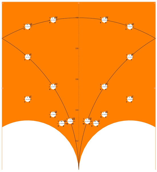
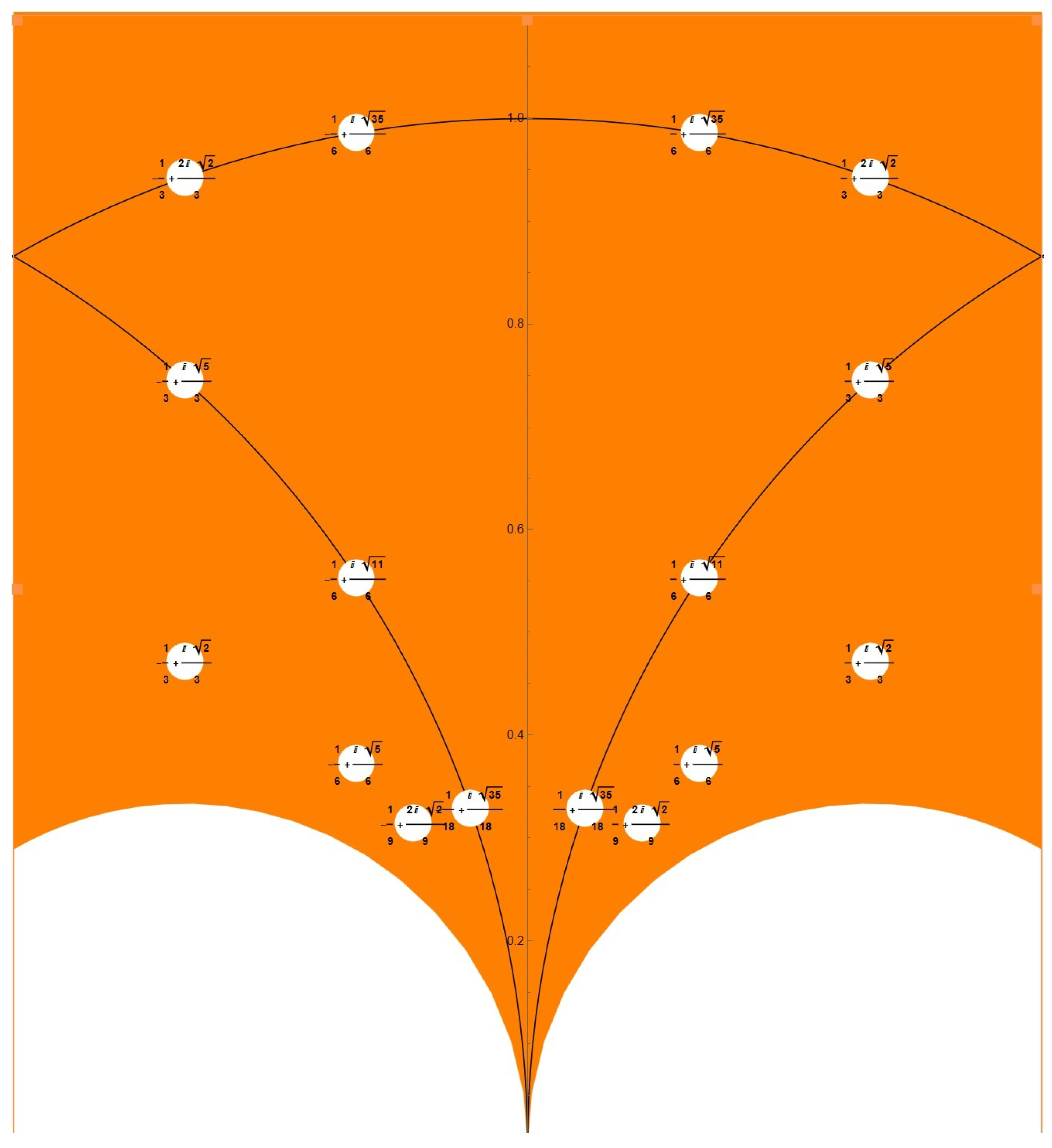
Using Kainberger’s program [19], the affine curve $Z_0\left(3\right)$ together with its non-cuspidal singular points is shown in Figure 1.

Figure 1. The plane model $Z_0\left(3\right)$ (the affine curve ${\mathrm{\Phi }}_3(X,Y)=0$) together with its non-cuspidal singular points (nodes). Each node corresponds to a collision of two distinct points of $X_0\left(3\right)$ under the map ${\mathrm{\Gamma }}_0\left(3\right)\tau \mapsto (j\left(\tau \right),j\left(3\tau \right))$, i.e., to a self-intersection coming from two non-equivalent 3-isogenies $E\to E^{\prime }$. The plot was generated using Kainberger’s program [19].

6. Discussion and Conclusions

As pointed out by Mazur in [2], the plane curve ${\mathrm{\Phi }}_N(X,Y)=0$ is highly singular, and its singular points determine points on the Jacobian of $X_0\left(N\right)$ defined over algebraic number fields. Precisely, if $(j\left({\tau }_1\right),j\left(N{\tau }_1\right))$ is a singular point on ${\mathrm{\Phi }}_N(X,Y)=0$, then $j\left({\tau }_1\right)$ and $j\left(N{\tau }_1\right)$ are algebraic numbers and there exists another point ${\mathrm{\Gamma }}_0\left(N\right){\tau }_2$ of $X_0\left(N\right)$ such that $(j\left({\tau }_1\right),j\left(N{\tau }_1\right))=(j\left({\tau }_2\right),j\left(N{\tau }_2\right))$ with ${\mathrm{\Gamma }}_0\left(N\right){\tau }_1\ne {\mathrm{\Gamma }}_0\left(N\right){\tau }_2$. In this paper, we designed an explicit enumeration algorithm for all non-cuspidal singular points of $Z_0(\ell )$ at the prime level and proved its termination and correctness.

The main practical limitations are the growth of class numbers for the encountered discriminants and the numerical precision required to certify equalities of singular moduli. There are several natural directions suggested by the present work. First, extending the enumeration from prime level ℓ to composite N is expected to require additional bookkeeping for decompositions of cyclic N-isogenies and potentially more complicated local intersection behavior of the plane model (compare the broader computational landscape around composite level and quotients in [5,6]). Second, it is natural to consider analogous questions for other modular curves (for instance $X_1\left(N\right)$ or modular curves attached to other congruence subgroups), where plane models and their singularities may encode different moduli identifications. Third, motivated by Mazur’s viewpoint, one may seek to explicitly compute the divisor classes arising from pairs of points $(P,Q)\in X_0\left(N\right)$ with $\pi \left(P\right)=\pi \left(Q\right)$ and to study their images under a Weil parametrization $\phi :X_0\left(N\right)\to E$, with the aim of producing algebraic points on E with special arithmetic properties; this fits naturally with recent database-scale work on modular curves and their Jacobians [10]. We hope to return to these questions in future work.

All the algorithms described in this paper have been implemented in Wolfram Language; for the programs, see [20].

References

- Washington, L.C. Elliptic Curves: Number Theory and Cryptography; Chapman and Hall/CRC: New York, NY, USA, 2008; p. 234. [Google Scholar]
- Mazur, B. Arithmetic of Weil curves. Invent. Math. 1974, 25, 1–61. [Google Scholar] [CrossRef] [Scilit]
- Anni, S.; Assaf, E.; Lorenzo García, E. On smooth plane models for modular curves of Shimura type. Res. Number Theory 2023, 9, 21. [Google Scholar] [CrossRef] [Scilit]
- Balakrishnan, J.S.; Dogra, N.; Müller, J.S.; Tuitman, J.; Vonk, J. Quadratic Chabauty for modular curves: Algorithms and examples. Compos. Math. 2023, 159, 1111–1152. [Google Scholar] [CrossRef] [Scilit]
- Adžaga, N.; Keller, T.; Michaud-Jacobs, P.; Najman, F.; Ozman, E.; Vukorepa, B. Computing quadratic points on modular curves X0(N). Math. Comput. 2024, 93, 1371–1397. [Google Scholar] [CrossRef] [Scilit]
- Bars, F.; González, J. Bielliptic modular curves. J. Algebra 2020, 559, 726–759. [Google Scholar] [CrossRef] [Scilit]
- Kunzweiler, S.; Robert, D. Computing modular polynomials by deformation. Res. Number Theory 2024, 11, 10. [Google Scholar] [CrossRef] [Scilit]
- Bröker, R.; Lauter, K.; Sutherland, A.V. Modular polynomials via isogeny volcanoes. Math. Comput. 2012, 81, 1201–1231. [Google Scholar] [CrossRef] [Scilit]
- Best, A.J.; Bober, J.; Booker, A.R.; Costa, E.; Cremona, J.E.; Derickx, M.; Lee, M.; Lowry-Duda, D.; Roe, D.; Sutherland, A.V.; et al. Computing classical modular forms. In Arithmetic Geometry, Number Theory, and Computation; Simons Symposia Series; Springer: Cham, Switzerland, 2021; pp. 131–213. [Google Scholar]
- Paulhus, J.; Sutherland, A.V. Completely Decomposable Modular Jacobians. Preprint 2025. Available online: https://lucant.org/papers/2025/250131-Sutherland.pdf (accessed on 28 January 2026).
- Kolyvagin, V.I. Finiteness of E(Q) and III(E/Q) for a subclass of Weil curves. Math. USSR-Izv. 1989, 32, 523–542. [Google Scholar] [CrossRef] [Scilit]
- Shimura, G. Introduction to the Arithmetic Theory of Automorphic Functions; Princeton University Press: Princeton, NJ, USA, 1971. [Google Scholar]
- Cox, D.A. Primes of the Form x2+ny2: Fermat, Class Field Theory and Complex Multiplication; John Wiley: Hoboken, NJ, USA, 1989. [Google Scholar]
- Klyachko, A.; Kara, O. Singularities of the Modular Curve. Finite Fields Their Appl. 2001, 7, 415–420. [Google Scholar] [CrossRef] [Scilit]
- Kara, O. Code Construction on Modular Curves. Ph.D. Thesis, Bilkent University, Ankara, Türkiye, 2003. [Google Scholar]
- Wang, S. On a theorem of Kara and Klyachko. Finite Fields Their Appl. 2025, 107, 102645. [Google Scholar] [CrossRef] [Scilit]
- Diamond, F.; Shurman, J. A First Course in Modular Forms; Springer: New York, NY, USA, 2005; pp. 38–40. [Google Scholar]
- Cohen, H. A Course in Computational Algebraic Number Theory; Springer: Berlin/Heidelberg, Germany, 1993; p. 234. [Google Scholar]
- Kainberger, P. Drawing Fundamental Domains, 2022. Available online: https://risc.jku.at/sw/drawfundoms/ (accessed on 12 December 2025).
- Wang, S. The Singularities of Z0(N). Available online: https://github.com/SanMinWang2025/An-algorithm-for-computing-the-singularities-of-the-plane-model-of-X0-N-/tree/main (accessed on 30 January 2026).
Disclaimer/Publisher’s Note: The statements, opinions and data contained in all publications are solely those of the individual author(s) and contributor(s) and not of MDPI and/or the editor(s). MDPI and/or the editor(s) disclaim responsibility for any injury to people or property resulting from any ideas, methods, instructions or products referred to in the content. |
© 2026 by the authors. Licensee MDPI, Basel, Switzerland. This article is an open access article distributed under the terms and conditions of the Creative Commons Attribution (CC BY) license.