Exploring the Use of Functional Data for Binary Classifications: The Case of Tissue Doppler Imaging in Cardiotoxicity Related-Therapy Cardiac Dysfunction Detection

Abstract

Functional data are nowadays routinely collected and stored in a wide variety of fields. Their adequate use and analysis are a challenge for the scientific community. Mathematically, each function can be understood as a sequence of infinite related numbers. Therefore, for statisticians, functional data can be read as a collection of a strongly correlated infinite-dimensional variable. Most existing statistical procedures have been adapted to functional data scenarios. In this manuscript, we are interested in understanding the use of functions for constructing adequate ROC curves and, therefore, for carrying out binary classifications. In particular, we consider the problem of studying the real capacity of functions derived from tissue doppler imaging (TDI) for identifying cardiac dysfunction related to cardiotoxicity therapy (CRTCD) in breast cancer women with high levels of the protein human epidermal growth factor receptor 2 (HER2). With this goal, we use public and freely available data that has been already used for illustrating the use of functional data in the binary classification problem with very different take-home messages. This variability in the conclusions made us question the reproducibility of the results. Here, we explore five different functional approaches, and we think about the clinical use of the provided solutions and their potential overfitting. The main aim of this manuscript is identifying whether published results are excessively optimistic or if they adequately capture the actual capacity of TDI for accurately diagnostic CRTCD.

1. Introduction

The binary classification problem (BCP) aims to correctly classify positive participants (with the characteristic under study) as positive and negative participants (without this characteristic) as negative. Conventionally, we have to make efficient use of the available information and define adequate classification rules. If we assume that the information is summarized in a continuous score, a (bio)marker, and that higher values of this score are associated with higher probabilities of being positive, the problem reduces to finding an adequate threshold, c, and classifying as positive those participants with a score value larger than c (the participants would be negative otherwise). Therefore, the interval $(c,\infty )$ would define ‘positiveness’ and would be our classification rule. Measures for associated errors include sensitivity ($S_E\left(c\right)$, the probability that a positive subject is correctly classified as positive); specificity ($S_P\left(c\right)$, the probability that a negative subject is correctly classified as negative); the positive predictive value (PPV(c), the probability that a subject declared as positive is actually positive); and negative predictive value (NPV(c), the probability that a subject declared as negative is actually negative).

The receiver-operating characteristic (ROC) curve [1] is a well-known graphical tool that represents the pairs $\{1-S_P\left(c\right),S_E\left(c\right)\}$ for each potential threshold $c\in \mathbb{R}$. Its theoretical and practical properties have been deeply considered in the literature (see, for instance, the monographs of Zhou et al. [2], Pepe [3], Krzanowski and Hand [4], or Nakas et al. [5], among others). Furthermore, the area under the curve, AUC ($={\int }_0^1\mathcal{R}\left(p\right)dp$, where $\mathcal{R}(·)$ is the ROC curve), is a popular index used to summarize in a single number the overall ability of the (bio)marker to correctly allocate subjects in the negative or positive group [6]. The ROC curve has been extended to time-dependent scenarios [7,8], non-monotone relationships between the score and the probability of being positive [9], or non-binary outcomes [10]. Different authors have considered the problem of constructing univariate scores that summarize the information contained in multivariate markers and get optimal ROC curves (see, for instance, Su and Liu [11] for a primer in the topic). Modern machine learning techniques have also been considered at this point [12,13], feeding the controversy between the accuracy and the interpretability of the resulting classification rules [14].

Functional data are, nowadays, routinely collected and stored in a wide variety of fields. Its practical use has become popular and includes a wide range of topics such as the precise positioning of a network of permanent global positioning system (GPS) stations [15]; learning how to reduce the energy consumption in buildings [16]; detecting deviations in the air quality [17]; or predicting the prevalence of COVID-19 [18]. In biomedicine, the application of FDA techniques is particularly appropriate, and its use has progressively increased over the last 25 years [19].

Functions can be seen as an infinite sequence of strongly related numbers. Therefore, for statisticians, functional data can be read as a collection of an infinite-dimensional variable. Functional data analysis (FDA) frequently considers the problem of using finite-dimensional techniques in infinite-dimensional scenarios. Most traditional statistical procedures have been adapted to accommodate functional data (FD). There is a number of excellent monographs that cover a great variety of topics. See, for instance, Ramsay and Silverman [20] for a general overview. Ferraty and Vieu [21] concern about non-parametric techniques. Theoretical and inferential aspects are considered in Horváth and Kokoszka [22] and Kokoszka and Reimherr [23]. Crainiceanu et al. [24] provides an extensive review of modern FDA methods with a very practical view, including implementation tools.

The ROC curve is not separated from this scenario. Escabias et al. [25] considered the use of functional principal component analysis (F-PCA) for proposing a functional generalized logit model in order to predict the group of the participants. The connection with ROC curve analysis is straightforward (a discussion about the use of logistic regression with functional data can be found in Aguilera et al. [26]). Estévez-Pérez and Vieu [27] explored the use of ranking functions via an adequate projection in an ordered subspace of these functions. The resulting procedure allows us to identify differences in the location parameter among functions, but cannot identify the groups when the main difference between them is with respect to the shape or the covariance structure. Bianco et al. [28] extended the idea of finding linear combinations for maximizing the AUC of the resulting punctuation to the FD framework. Furthermore, they introduced a quadratic component, which allows us to improve the quality of the prediction. Martínez-Camblor [29] proposed the use of the area under the generalized ROC curve, gAUC [30], for estimating the probability of each curve to be positive and then to use these probabilities as a final classifier. The last two manuscripts considered the same data example for illustrating their proposals. However, the provided overall classification accuracies were considerably different. While the quadratic procedure proposed by Bianco et al. [28] reached an AUC of 0.89 (their linear procedure reported an AUC of 0.71), the probability-based criterion, PBC, proposed by Martínez-Camblor [29] got a poor AUC of 0.60, and this was reduced to an average AUC of 0.54 after overfitting correction (based on 200 replicates of a standard training–testing procedure). This discrepancy motivated this research, whose main goal is understanding the real capacity of tissue doppler imaging (TDI) for identifying cardiac dysfunction related to cardiotoxicity therapy (CRTCD). From a methodological perspective, here, we do not introduce new classification methods based on functional data. Our main goal lies instead in a critical reassessment of existing approaches applied to this specific dataset. The key methodological contribution of this paper is the explicit emphasis on overfitting problems, addressed through repeated training–testing procedures and supported by a targeted Monte Carlo simulation study.

The rest of the paper is organized as follow. In Section 2, we present the data and motivate this research. Section 3 contains the main mathematical notation and theoretical considerations. We reduce the problem from functions (infinite) to multivariate analysis and explore the performance of this discretization in Section 4. In Section 5, we directly use linear and quadratic forms of the F-PCA procedure proposed by Escabias et al. [25] and implemented in Escabias et al. [31] to feed a logistic regression predictive model. The procedure introduced by Martínez-Camblor [29] is considered in Section 6. Trying to have a better understanding of the performance of these functional techniques, we conducted a small Monte Carlo simulation study, whose results are provided in Section 7. Section 8 summarizes the results of our analyses, while some discussion and main conclusions are included in Section 9. Interested readers can find the R code (R Studio Version 4.5.1) at the following github address: https://github.com/PabloMartinezCamblor/Discriminatory-ability-of-tissue-doppler-imaging (accessed on 2 February 2026).

2. Motivation

In order to illustrate the practical behavior of their proposal, Bianco et al. [28] considered the problem of using the functions derived from tissue doppler imaging (TDI) for identifying cardiac dysfunction related to cardiotoxicity therapy (CRTCD) in breast cancer women with high levels of the protein human epidermal growth factor receptor 2 (HER2) treated with drugs specifically targeting this HER2 protein. 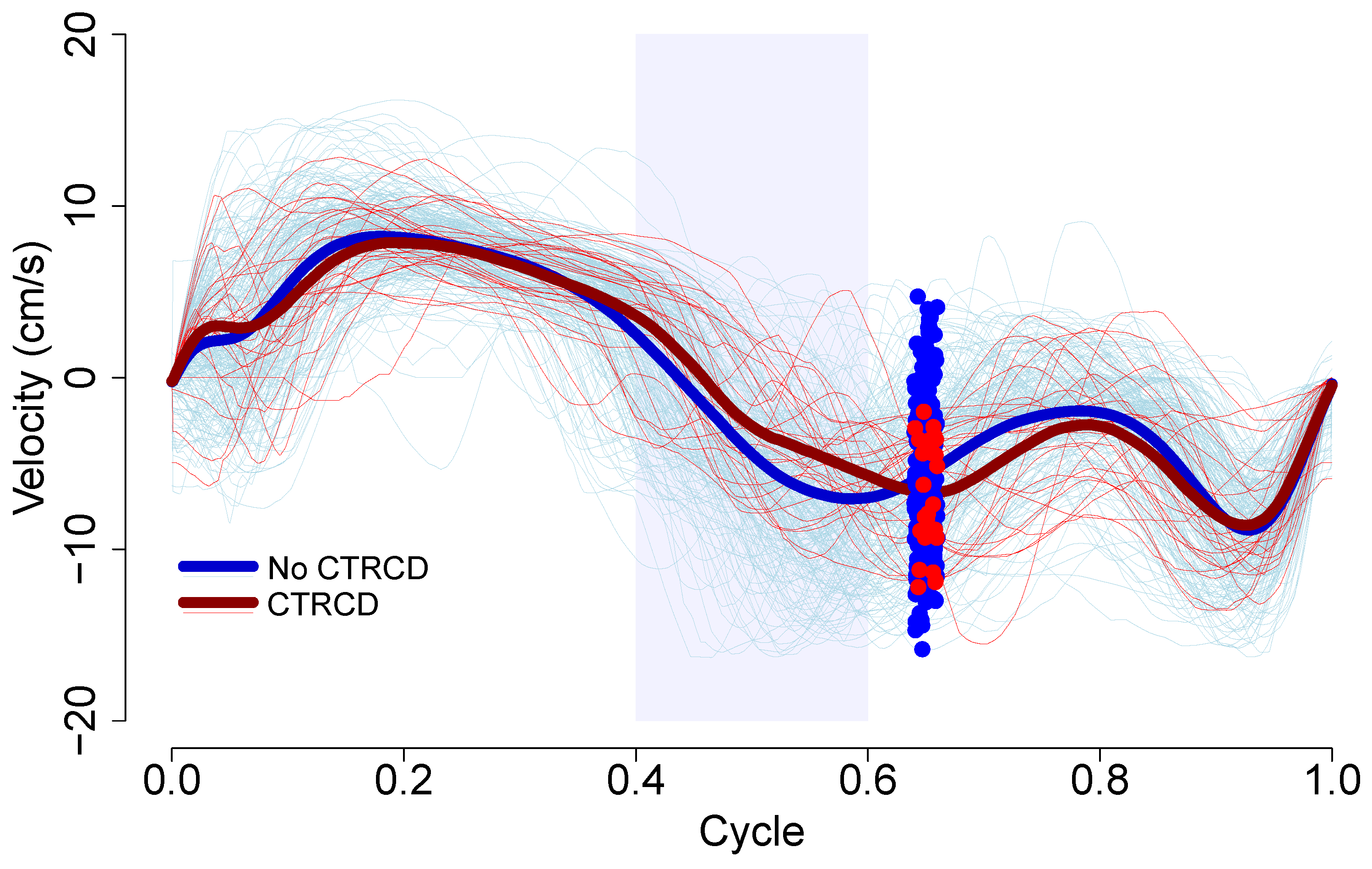The dataset used, including a total of 270 independent functions (27 from positive women), is deeply described in [32] and can be freely downloaded at https://doi.org/10.6084/m9.figshare.22650748.v4. When we stared at the resulting functions (Figure 1), we observed that the blue area dominates the space up and down (we realize that the number of functions in blue is larger), suggesting a non-monotone relationship between TDI and CRTCD. When we use the values of the functions at one (more or less) random selected point (here, Cycle = 0.65) for classifying the subjects, the resulting gROC curve has an associated gAUC of 0.70 (95% CI: 0.61 to 0.79). However, we have the impression that we are misusing most of the available information. For instance, we can also see that negative functions (tend to) have lower values than positive functions when Cycles are between 0.4 and 0.6. Let us use the minimum value of the functions within this period for doing the classification. The obtained AUC is then 0.71 (95% CI: 0.63 to 0.81). Although this is separate from the objective of this manuscript, the biological explanation of these criteria could be easily discussed with clinicians, who could find (or not find) some rationality behind the results. Furthermore, the potential effect of other demographics and/or clinical covariates could explain (or modulate) the predictive capacity of the models. Responding to this question would involve different type of analyses, including covariate-specific ROC curves [33].

Both criteria provide moderate results (far from the AUC of 0.89 reached in Bianco et al. [28]). Furthermore, the considered classifications were defined ad hoc (we chose the best ones based on our intuition after visual inspection of the curves; these effects could be mitigated if we could find some biological justification), with the underlying risk of overfitting. Some direct questions arise. Does TDI contain enough information about CRTCD for doing accurate diagnostics? That is, could we use the available information in a more effective way without incurring overfitting? Could we provide understandable rules for knowing whether a curve is from a CRTCD-positive or from a CRTCD-negative woman?

In the next section, we introduce the mathematical framework behind the general problem of using functional data for binary classifications.

3. Theoretical Considerations

Let $\mathcal{F}$ be the $L^4\left(T\right)$ space (the justification of the functional space is provided in the Remark 1 at the end of this section), that is, a separable Hilbert space such that each $f\in \mathcal{F}$ is a function, $f:T\to \mathbb{R}$ satisfying ${\int }_{T}f{\left(t\right)}^{4}dt<\infty$. Let ${\mathcal{F}}_N$ and ${\mathcal{F}}_P$ be a partition of $\mathcal{F}$ representing the negative ($Y=0$) and the positive ($Y=1$) trajectories, respectively.

We are looking for an adequate operator, $\Psi :\mathcal{F}\to \mathbb{R}$, that it optimizes $\mathbb{P}\{\Psi \left({\mathcal{F}}_N\right)<\Psi \left({\mathcal{F}}_P\right)\}$, where $\Psi \left({\mathcal{F}}_k\right)=\{\Psi \left(f\right):f\in {\mathcal{F}}_k\}$ ($k\in \{N,P\})$. Potential definitions of $\Psi$ include ${min}_{0.4\le t\le 0.6}\left\{f\left(t\right)\right\}$ or $f\left(0.65\right)$. Other simple (and useful) definitions can be found in Jang and Manatunga [34]. A functional ROC curve associated with the operator $\Psi$ is defined by

$${\mathcal{R}}_{\Psi }\left(p\right)=1-F_{\Psi \left({\mathcal{F}}_P\right)}\left(F_{\Psi \left({\mathcal{F}}_N\right)}^{-1}(1-p)\right),1\le p\le 1,$$

(1)

where $F_{\Psi \left({\mathcal{F}}_k\right)}(·)=\mathbb{P}\{\Psi \left(f\right)\le ·:f\in {\mathcal{F}}_k\})$, for $k\in \{N,P\}$.

Let $\{f_1,\cdots ,f_{n_0},f_{n_0+1},\cdots ,f_{n_0+n_1}\}$ be n ($=n_0+n_1$) independent random functions drawn from $\mathcal{F}$ (the first $n_0$ from ${\mathcal{F}}_N$, the remaining $n_1$ from ${\mathcal{F}}_P$). When $\Psi$ is absolutely specified, we can define the empirical estimator of $F_{\Psi \left({\mathcal{F}}_N\right)}$ (and, analogously, for $F_{\Psi \left({\mathcal{F}}_P\right)}$) by

$${\widehat{F}}_{\Psi \left({\mathcal{F}}_N\right)}(·)={\displaystyle \frac{1}{n_0}}\sum _{i=1}^{n_0}\mathbb{I}\{\Psi \left(f_i\right)\le ·\},$$

where $\mathbb{I}\left\{A\right\}$ takes the value 1 if A is true and 0 otherwise (following conventional statistical criteria, we denote the estimator by adding a hat over the quantity to be estimated). The resulting empirical ROC curve estimator, ${\widehat{\mathcal{R}}}_{\Psi }(·)$ (and its associated AUC), inherits the theoretical properties studied in Hsieh and Turnbull [35]. However, when $\Psi$ itself has to be estimated, we have to cope with different problems. (1) If we use the same dataset for estimating both $\Psi$ and ${\mathcal{R}}_{\Psi }$, we will probably obtain over-optimistic results (overfitting); (2) if we implement a training–testing approach, in which a portion of the data is used for estimating $\Psi$, while the ROC curve is estimated with the remaining data, we will obtain an appealing estimator for

$${\mathcal{R}}_{\widehat{\Psi }}\left(p\right)=1-F_{\widehat{\Psi }\left({\mathcal{F}}_P\right)}\left(F_{\widehat{\Psi }\left({\mathcal{F}}_N\right)}^{-1}(1-p)\right),1\le p\le 1,$$

where $\widehat{\Psi }$ is the estimation of $\Psi$ based on the training sample, instead of having an estimation of our original target ${\mathcal{R}}_{\Psi }$. (3) Results of the training–testing approach will be affected by the randomness in the selection of training and testing sub-samples.

Remark 1.

Usually, it is enough to ask that ${\int }_T{f}^2\left(t\right)dt<\infty$ ($L^2\left(T\right)$ space). However, the nature of the observed differences between the curves in the negative and positive groups anticipates the presence of a quadratic structure. We are interested in using the curves $f^2$ as predictors. We want these functions among the eligible curves. Therefore, we have to ask that $f^2\in \mathcal{F}$, and then ${\int }_T{\left(f^2\left(t\right)\right)}^{2}dt={\int }_T{f}^4\left(t\right)dt<\infty$; that is $\mathcal{F}=L^4\left(T\right)$.

Remark 2.

Without loss of generality, we can assume that $f\in \mathcal{F}$ is

$$f\left(t\right)={\mathit{g}}_k\left(t\right)+{\tau }_k\left(t\right),\mathit{for}k\in \{N,P\},$$

with ${\mathit{g}}_k$ the average function in ${\mathcal{F}}_k$, and $\mathbb{E}\left[{\tau }_k\left(t\right)\right]=0\forall t\in T$ ($k\in \{N,P\}$). Delaigle and Hall [36] explored the properties of the centroid method in the functional data context and concluded that, under certain circumstances, it would reach near-perfect asymptotic accuracy. In our problem, the centroids, ${\mathit{g}}_N$ and ${\mathit{g}}_P$, look similar (thick lines in Figure 1), and based on the amount of observed noise, ${\tau }_k$ ($k\in \{N,P\}$), near-perfect accuracy, is unlikely. There are a number of works dealing with the overall classification problem and functional data (see Wang et al. [37] for a complete and recent overview). However, and despite the clear connections between the general classification problem and the ROC curve construction (overall when the classification process reaches near-perfect accuracy), we want to highlight that both scenarios are not the same.

4. Exploring Discretized Functions

Binary regression models are routinely used for reducing multivariate markers in a real-value score. For instance, considering the logit as a link function ($\mathrm{logit}\left(x\right)=log[x/(1-x\left)\right]$, for $x\in (0,1)$), we fit the model

$$\mathrm{logit}\left[\mathbb{P}\{Y=1|\mathit{X}=x\}\right]={\alpha }_0+\sum _{i=1}^s{\alpha }_i·x_i,$$

where $\mathit{X}=\{X_1,\cdots ,X_s\}$ is an s-dimensional random variable, and $\mathit{x}=\{x_1,\cdots ,x_s\}$ is one particular value. After estimating the $s+1$ involved parameters, ${\beta }_0,{\beta }_1,\cdots ,{\beta }_s$ (we can avoid the intercept ${\beta }_0$), the resulting unidimensional score is modeled by the random variable ${\sum }_{i=1}^s{\alpha }_i·X_i$. This procedure is easily generalizable to a non-linear relationship between the marker and the outcome and also to the functional context:

$$\begin{array}{cc}\hfill \mathrm{logit}\left[\mathbb{P}\right\{Y=1|\mathcal{F}=f\}]=& {\alpha }_0+{\int }_T\beta \left(t\right)f\left(t\right)dt+{\int }_T\gamma \left(t\right)f^2\left(t\right)dt\hfill \\ \hfill \approx & {\alpha }_0+\sum _{i=1}^L\beta \left(t_i\right)f\left(t_i\right)+\sum _{i=1}^L\gamma \left(t_i\right)f^2\left(t_i\right),\hfill \end{array}$$

where $\{t_1,\cdots ,t_L\}$ is a sequence of points within the interval T. The last expression is a raw approximation, and its quality would depend on several things, including the number of points L. Furthermore, the correlation between the values of the functions (and their square) could be a source of multicollinearity, especially for large values of L. In order to reduce this multicollinearity, we can use a method for dimensional reduction such as the popular principal component analysis, PCA.

In the PCA analysis [38], we take advantage of the correlation matrix properties (symmetry and positive definite) associated with the s-dimensional marker and compute the singular value decomposition

$$\mathit{X}=\mathit{U}·\mathit{D}·{\mathit{V}}^T,$$

where $\mathit{X}$ is the $n\times s$ matrix containing the typified values of the sample (n observations, s variables), and $\mathit{D}$ is the $s\times s$ diagonal matrix formed by the sorted eigenvalues of $\mathit{C}$ (correlation matrix: $\mathit{C}=\mathit{X}·{\mathit{X}}^t/(n-1))$. The matrices $\mathit{U}$ ($n\times s$) and $\mathit{V}$ ($s\times s$) are the left and right singular vector matrices, respectively.

The original s-dimensional marker admits the representation $\mathit{F}=\mathit{X}·\mathit{V}$, where the s-components contained in $\mathit{F}$ are orthogonal (independent) and sorted by relevance according to the proportion of variance retained. Conventionally, we extract a number of them based on a predefined criterion (e.g., eigenvalues larger than one, or the first K satisfying that ${\sum }_{i=1}^K{\lambda }_i/s>P$, for a particular $P\le 1$, typically $P=0.6$). Each component is a linear combination of the original variables. Based on the weights and nature of these variables, we can determine in turn the nature of each component (e.g., the first values of the Cycle, etc.).

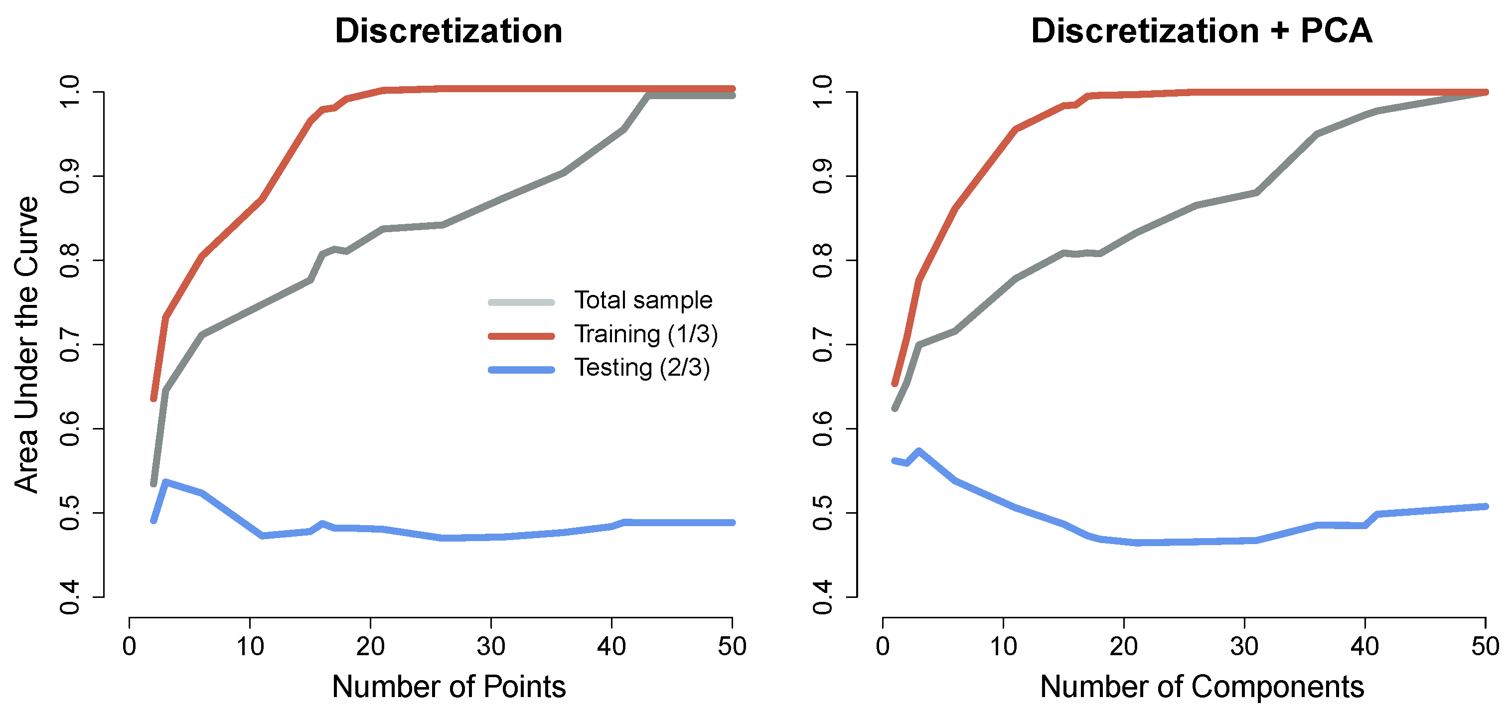
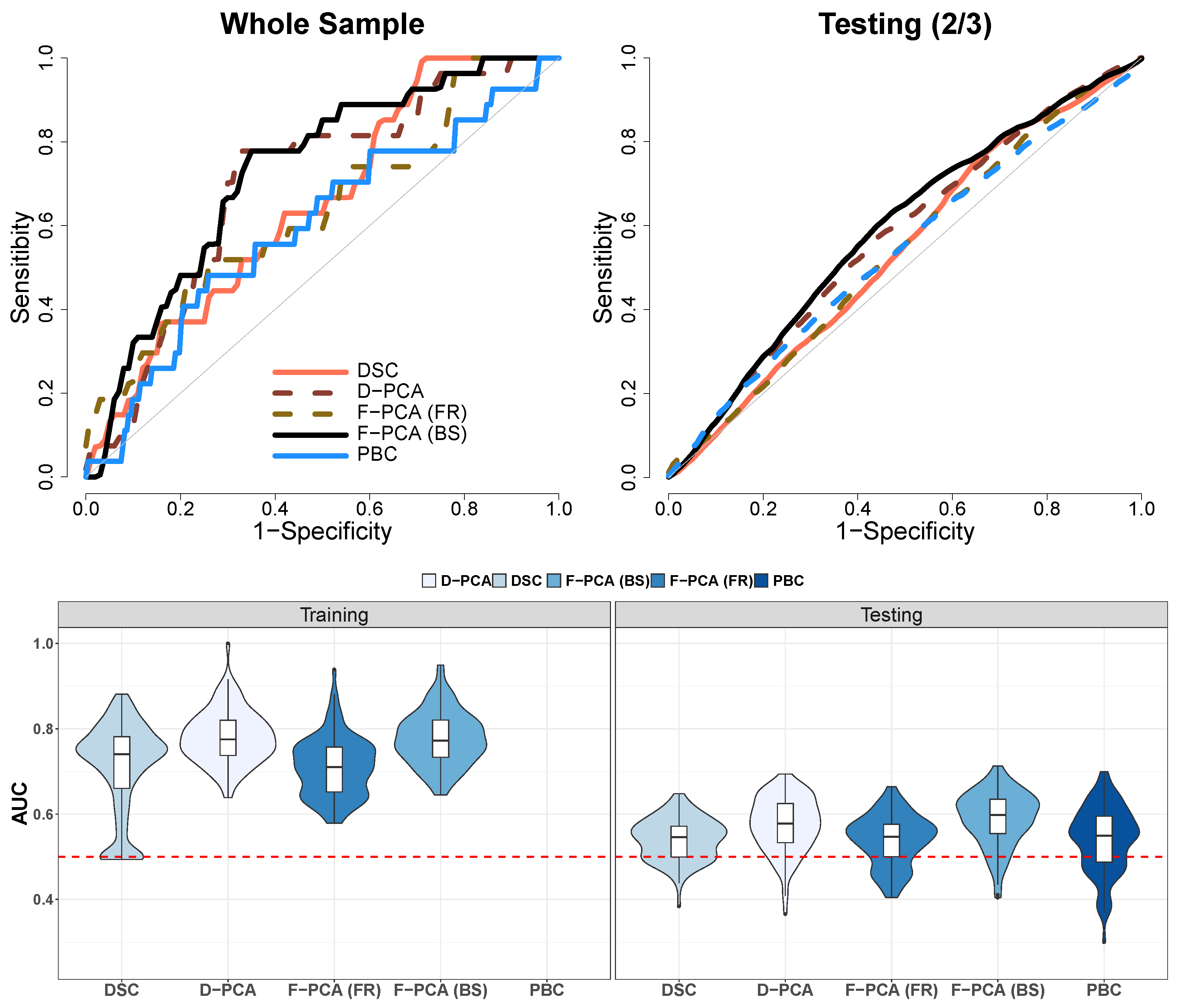
Once we decide the number, K, of variables to be used (these variables are those resulting in the discretization process (DSC), or the first K-components from the PCA based on a more exhaustive discretization, D-PCA), we fit a binary model with the $2·K$ (K from the straight and K for the quadratic functions) selected variables. However, we know that this process adds overfitting to the marker [39]. In order to control this overfitting, we performed a calibration process and computed the accuracy of both the DSC and the D-PCA procedures when we apply them to the whole sample and on a training–testing procedure (approximately 1/3 of the sample used for training and remaining 2/3 for testing; we report average results based on 100 replicates) for different values of K (see Figure 2).

When we applied the DSC algorithm to the whole sample, we reached an AUC of 0.91 for $K=36$, and for $K=43$, the AUC was 1. In the training cohort, we only need 11 and 21 points to reach average AUCs of 0.90 and 1, respectively. Unfortunately, the testing cohort got a maximum average AUC of 0.53 for $K=3$ (Figure 2-left). The D-PCA results were similar; on the whole sample, $K=31$ reached an AUC of 0.88, and $K=50$ an AUC of 1. For the training sample, 10 and 19 components reached average AUCs of 0.89 and 1, respectively. The maximum average AUC for the testing cohort was 0.58, and it again reached $K=3$ (Figure 2-right).

In a visual inspection of the three-component solution, we learn that large values in the first component of the functions are associated with higher values at a Cycle between 0.23 and 0.44 and lower values between 0.58 and 0.68. The second component takes higher values in those curves with low values in a Cycle between 0.44 and 0.58 and high values between 0.68 and 0.89. Finally, the third component takes larger values for curves taken high values at the beginning (a Cycle between 0.05 and 0.25).

The two procedures discussed in this section represent a naive approximation to the problem. Since, in practice, we cannot collect continuous information, DSC explores the use of an adequate (less bad) discretization process; that is, to choose a finite collection of points to characterize the functions. The main parameter to select is, therefore, the points. We have considered an equal number of them. We determined the final number by bootstrapping. The second procedure, D-PCA, is similar to the previous one, but, instead of restricting the number of points in the discretization process, it tries to retain the most relevant information from implementing a standard PCA procedure. The parameters to select are the original number of points to be included in the PCA (less relevant than in DSC and assumed to be large enough) and then the number of PCA components to include in the logistic model. The final number of components is determined again by bootstrapping.

Remark 3.

The proportion used in the training–testing approach was 1/3–2/3. The relevance of this proportion has already been considered in the literature (e.g., Vrigazova [40]). It represents a trade-off between the variability in the classification criterion, computed with the training sample, and the variability in the estimation of the accuracy, estimated with the testing sample. Since we are reporting averages obtained in a number of iterations, the results are very robust and do not depend on the ratio.

Remark 4.

Given the weakness of the classification observed in these procedures, we have not gone further in the interpretation of the models. However, we want to highlight that the analysis of the coefficients involved in the binary regressions helps to understand the weights and which points have relevance in the classification process. Clinicians should compare the biological interpretation (sound) to the resulting classification criteria.

5. Using Functional PCA

This procedure is based on selecting an adequate basis of functions for the considered functional space, $L^4\left(T\right)$, $\{B_1\left(t\right),\cdots ,B_L\left(t\right)\}$, and projecting the observed functions in this base. That is, each function $f\in \mathcal{F}$ is represented by the L-dimensional real vector $(a_1,\cdots ,a_L)$ that satisfies

$$\begin{array}{c}\hfill f\left(t\right)\approx a_1·B_1\left(t\right)+\cdots a_L·B_L\left(t\right),t\in T.\end{array}$$

This representation reduces the original infinite-dimensional problem to a more standard L-dimensional one. Different bases such as B-splines or wavelets, among others, can be considered with this goal. In our case (following Bianco et al. [28]), we consider Fourier series. Therefore, we assume that each function $f\in \mathcal{F}$ can be expressed in the form

$$\begin{array}{cc}\hfill f\left(t\right)=& {\alpha }_0+\sum _{i\in \mathbb{N}}\left\{{\beta }_i·sin(2\Pi ·i·t)+{\gamma }_i·cos(2\Pi ·i·t)\right\}+ϵ\left(t\right)\hfill \\ \hfill \approx & {\alpha }_0+\sum _{i=1}^L\left\{{\beta }_i·sin(2\Pi ·i·t)+{\gamma }_i·cos(2\Pi ·i·t)\right\},\hfill \end{array}$$

for adequate coefficients ${\alpha }_0$ and ${\{{\beta }_i,{\gamma }_i\}}_{i\in \mathbb{N}}$, with $ϵ\left(t\right)$ as an error function. The quality of the approximation in the second line of the above equation strongly depends on the selection of the natural number L and on the ability of the basis for representing the functional space $\mathcal{F}$. Once we have fixed L, each function is determined by its associated coefficients $({\alpha }_0,{\beta }_1,\cdots {\beta }_L,{\gamma }_1,\cdots {\gamma }_L)$. Given the dependency of the functional basis, we also explore the implementation of a B-spline (cubic spline) representation [41]. However, as in the procedures described in the previous section, the risk of multicollinearity in these procedures increases with L. Hence, it is advisable to complement it with a dimension-reduction procedure. Notice that, based on the structure of the curves in our problem, we have to approximate not only f, but also $f^2$. The algorithm that we finally implement is as follows.

• Select a functional basis with a large enough value of L for allowing an adequate representation of the functions in the sample. For each function in the sample, $f_i$ ($1\le i\le n$), compute the coefficients associated with both $f_i$ and $f_i^2$, on this basis.
• Compute two PCA analyses on the two sets of coefficients, and select an adequate number of component scores, K.
• Fit a logistic regression model including the selected component scores.
• Use the resulting punctuation as a marker.

The number of (component) scores to be finally included in the logistic model can be a controversial decision. In the sake of simplicity, we have opted for selecting the same number of components in both the linear and the quadratic function representations (Step 2), but this number could be different. Furthermore, the final number of covariates included in the logistic model is therefore $2·K$, and as we mentioned in the previous section, the overfitting of the model increases drastically with K [39]. 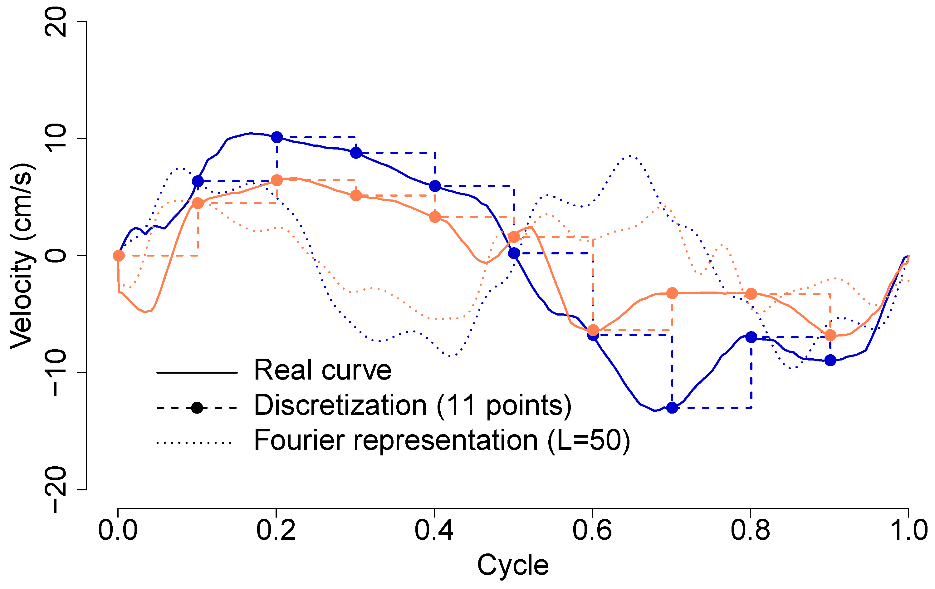Figure 3 shows the quality of the Fourier representation based on $L=50$ for two functions randomly selected from our CRTCD data (one from the negative and the other from the positive populations, in blue and red, respectively). We also show the representation of the curves for the discretization based on 11 points with the associated stepwise function. Fourier representations are not even similar to the original curves, suggesting that this basis is not the most appropriate for our problem. However, a B-splines representation with $L=50$ perfectly matches with the real curves.

When we consider the whole sample for constructing the classification rules (representation based on Fourier series, $L=50$), the accuracy strongly depends on the number of principal components we are including in the logistic model. The F-PCA algorithm reaches an AUC of 0.9 for $K=36$ and a perfect classification (AUC = 1) for $K=49$. The optimism is curved down when we implement a training–testing algorithm (approximately 1/3 of the sample for training and the remaining 2/3 for testing, and we report the average based on 100 replicates of this process); the AUC in the training sample is 1 for 26 components, but the results on the testing sample reach a maximum AUC of 0.53 for $K=3$. Similar results were observed when we consider a B-spline representation ($L=50$). For the whole sample, the procedure reaches an AUC of 0.9 for $K=32$, and an AUC of 1 for $K=46$. In the training–testing procedure, the AUC in the training sample is 1 for $K=19$. The maximum AUC in the testing sample was 0.60 for $K=3$.

In summary, the F-PCA procedure requires to select, initially, a basis of functions for representing the elements in $\mathcal{F}$, and then, to choose the number of components to be used in the predictive model. We explored the use of two different popular basis (Fourier series and B-splines), which show a different capacity for representing the curves but got a similar classification accuracy. The number of components was automatically selected by bootstrapping.

6. The PBC Approach

The probability-based classification criterion (PBC) [29] identifies each function with its probability of being positive and then uses these probabilities (which become the marker) for constructing the ROC curve. For computing the marker, for each function $f\in \mathcal{F}$, the procedure is based on the distances between f and rest of the functions. That is, theoretically, for a fixed $f\in \mathcal{F}$, we consider the random variable

$$X_f=\{d_g:={\int }_T{(f\left(t\right)-g\left(t\right))}^{2}dt:g\in \mathcal{F}\}.$$

The underlying reasoning is that functions from the positive subjects are closer to functions from other positive subjects than to those from the negative group. However, since within one group we could observe different behaviors, we allow a more flexible use of these distances and compute the probability

$$\mathbb{P}\{h_f\left(X_{f,N}\right)<h_f\left(X_{f,P}\right)\},$$

where $X_{f,k}=\{d_g:={\int }_T{(f\left(t\right)-g\left(t\right))}^{2}dt:g\in {\mathcal{F}}_k\}$ ($k\in \{N,P\}$), and $h_f$ is an adequate transformation. The proposed transformation, $h_f$, is associated with the gROC curve [42], and therefore, the above probability would be the gAUC [30]. For more information about the estimation of $h_f$, interested readers are referred to Martínez-Camblor and Pérez-Fernández [43]. The package nsROC [44] implements the described techniques.

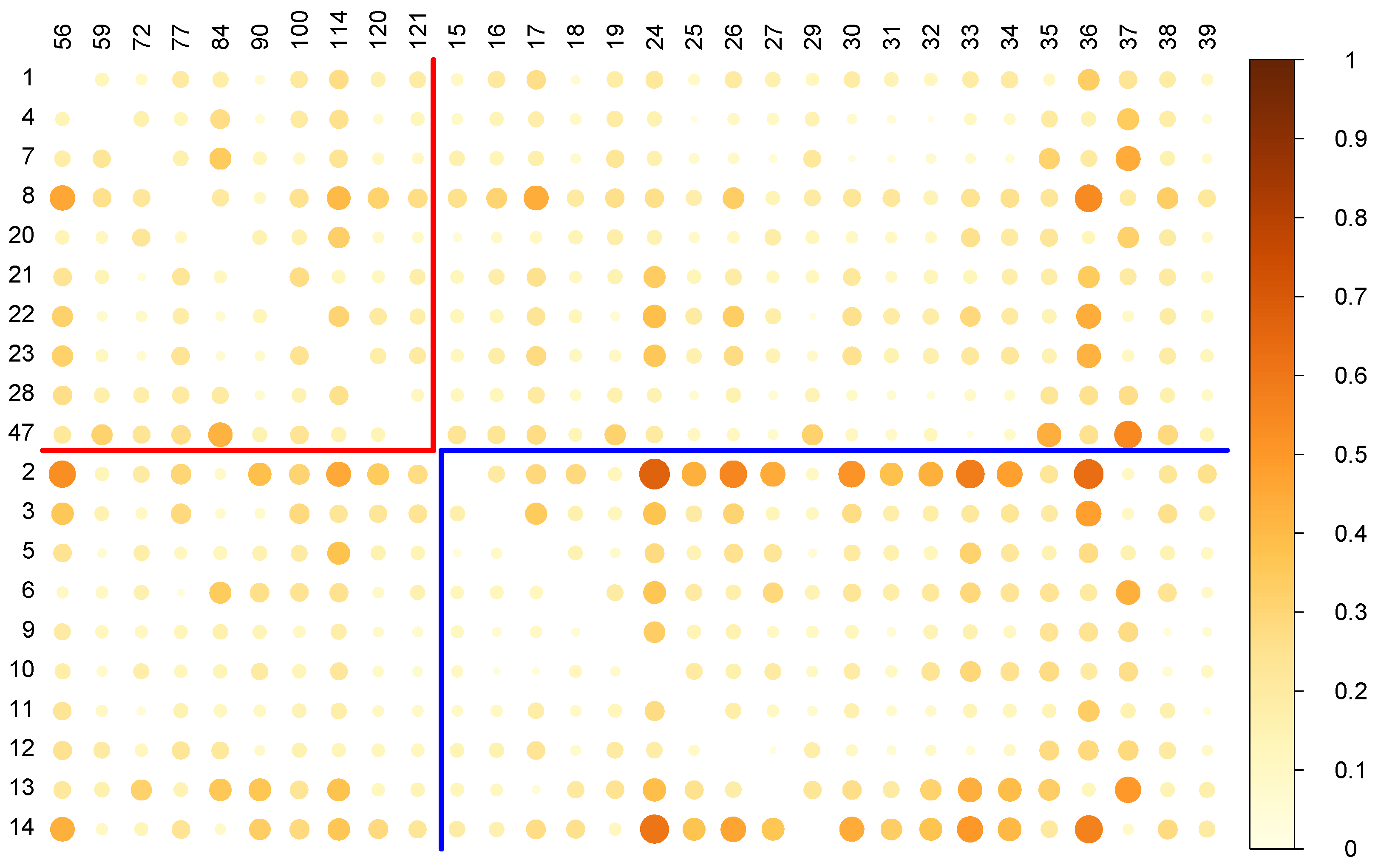
The PBC success is, of course, strongly related to the behavior of the distances between the negative, and the positive curves, which we assume to be different. Figure 4 shows the relative distance (we ranked the real distance to be within the interval [0, 1]) between 20 random functions, 10 from the negative, and 10 from the positive group (labeled in the y-axis), and another 30 different random functions, 20 from the negative, and 10 from the positive (labeled in the x-axis). The observed distances reduce the expectations about the potential quality of the classification. Positive–positive (top-left square) distances are not particularly different to the positive–negative distances (top-right square). A similar pattern is observed when we compare negative–negative (bottom-right square) and negative-positive distances (bottom-left square).

As we mentioned in the introduction of this paper, when we apply the PBC procedure to the whole sample, we see reflected the similar behavior between the distances, and the AUC reached was 0.60. This result is even worse when we apply the more reliability training–testing procedure based on randomly selecting (approximately) 1/3 of the sample for training, and the remaining 2/3 for testing, and we reach an average (based on 100 iterations) AUC of 0.55 (this result is on the testing sample, we do not have AUCs for the training sample in this procedure).

PBC method is free of the selection of controversial parameters. Perhaps the critical decision to take is the estimation of $h_f$, although we deferred this to an automatic algorithm fully described in Martínez-Camblor and Pérez-Fernández [43].

Remark 5.

The slightly difference between the results reported in the current training–testing process, an average AUC of 0.55 based on 100 replications, and the result reported in Section 1, an average AUC of 0.54 based on 200 replications, is because we are replicating our own results here. The randomness produces these small differences.

7. Some Monte Carlo Simulations

In order to have a better understanding of the real capacity of the above procedures for correctly identifying the ability of functional information to discriminate between negative and positive subjects under the circumstances considered, we carried out a small Monte Carlo simulation study informed by our real problem. We highlight that the goal is not to compare or study the overall performance of the procedures but to understand their behavior within the considered data structure. Readers interested in having more feedback about the overall performance of these techniques are referred to Martínez-Camblor [29]. In the Scenario I and Scenario II considered, the functions do not provide information about the condition (negativeness/positiveness) of the subjects. We generate $f_i\left(t\right)=\mathit{g}\left(t\right)+{\tau }_i\left(t\right)$ for $1\le i\le n$ ($n=n_0+n_1$), where $\mathit{g}$ is the average of the 270 functions included in the CRTCD data. In the Scenario I,

$${\tau }_i\left(t\right)={\alpha }_0+\sum _{j=1}^{10}\left\{{\beta }_j·sin(2\Pi ·j·t)+{\gamma }_j·cos(2\Pi ·j·t)\right\},$$

where $({\alpha }_0,{\beta }_1,\cdots ,{\beta }_{10},{\gamma }_1,\cdots ,{\gamma }_{10})$ is a 21-dimensional random vector following the distribution ${\mathcal{N}}_{21}(\mathit{a},\Sigma )$, with $\mathit{a}$ and $\Sigma$ computed from the mean vector, and the covariance matrix of the Fourier representation of the residuals derived from the CRTCD data. In the Scenario II, ${\tau }_i$ is generated following a scaled Brownian Bridge process. The Scenario III and Scenario IV were generated analogously to scenarios I and II, respectively, but the average function $\mathit{g}$ involved mean vectors, and covariance matrices were computed separately from the negative and the positive curves. In both scenarios, differences between the covariance matrices were slightly exacerbated (the scheme considered is supposed to have larger AUCs than those based on the original data). The full R code, and figures representing random sets of curves for each model can be accessed at https://github.com/PabloMartinezCamblor/Discriminatory-ability-of-tissue-doppler-imaging (accessed on 2 February 2026).

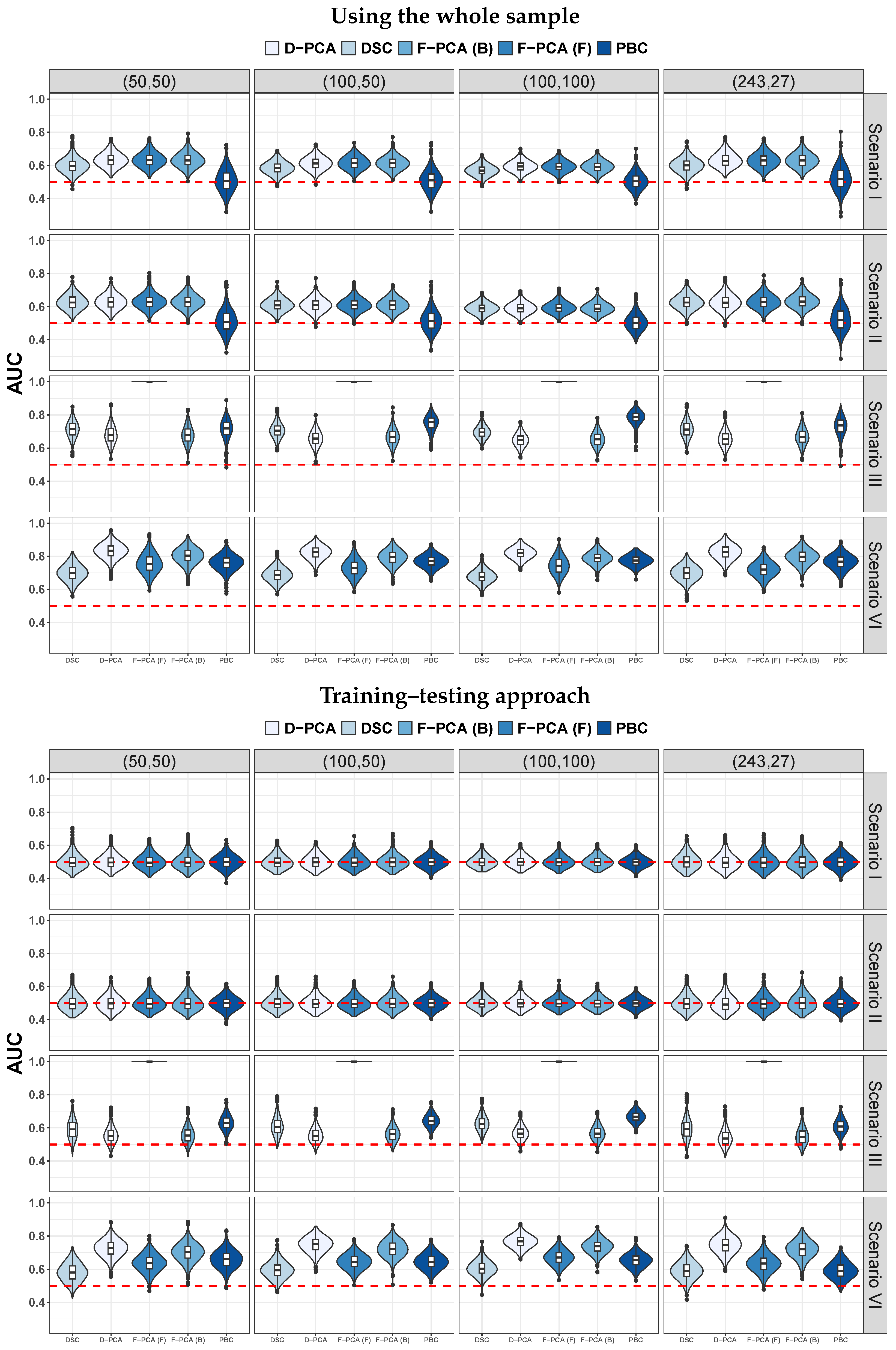
Figure 5 contains violin and box plots for the AUCs obtained in 1000 Monte Carlo iterations of the four models described above and for four different sample sizes configurations, $(n_0,n_1)=(50,50),(100,50),(100,100)$ and $(243,27)$. The estimation procedures considered include the direct discretization discussed in Section 4, DSC (based on the calibration process, we included only three points); the PCA analysis based on 101 discretization points of the curves, D-PCA (based on the calibration process, we included only the first three components), the functional principal components procedure described in Section 5 based on the first 101 coefficients of the Fourier representation of the curves, F-PCA (F) and on 50 coefficients of a B-spline basis, F-PCA (B) (again, based on the calibration process, we only included three components); and the PBC algorithm described in Section 6. Furthermore, we report results for an estimation process based on the whole sample and for the average AUCs (based on 10 iterations) of a training–testing procedure using approximately 1/3 of the sample for training and the remaining 2/3 for testing.

Results confirm that when we use the whole population, we get overly optimistic conclusions for all the procedures but PCB, which shows more variability than the other procedures in the four models, but whose average AUCs in Scenarios I and II were around 0.5. We can confirm as well that the training–testing approach provides a more realistic knowledge of the underlying reality. In Scenario III, the F-PCA (F) reached a perfect classification (AUC = 1), while the other four estimation methods behaved similarly (notice that, in this scenario, curves were generated following a Fourier series structure and, in this context, F-PCA (F) almost becomes a parametric procedure). In the Scenario IV, D-PCA and PBC were the winners when we applied the procedures to the whole sample. However, in the training–testing procedure, PBC is more sensitive to the sample size reduction and, in particular, to the small number of positive curves in the last configuration (only 27 positive curves), especially when we implement the training–testing procedure. In this case, positive profile is based on only around nine positive curves, and in this sample size configuration, PBC performance is similar to and even worse than DSC, F-PCA (F) and F-PCA (B).

8. Summarizing Results

In this section, we summarize the results observed when we apply the five considered methods to the CRTCD data.

Table 1. AUCs. AUCs for the five procedures considered (including F-PCA with Fourier representation (FS) and B-splines (BS)) using the whole sample (total) and the described training–testing procedure (averages based on 100 replicates).

	Total	Training	Testing (95% CI)
DSC (3 points)	0.65	0.69	0.53 (0.41 to 0.65)
D-PCA (3 components)	0.70	0.79	0.58 (0.47 to 0.69)
F-PCA (FR) (3 components)	0.64	0.73	0.53 (0.41 to 0.65)
F-PCA (BS) (3 components)	0.73	0.78	0.60 (0.50 to 0.70)
PBC	0.60	—	0.55 (0.43 to 0. 67)

shows the AUCs when these methods are applied on the whole sample (Total) and when we apply a training–testing procedure using approximately 1/3 of the sample for training, and the remaining 2/3 for testing. In this case, the reported AUCs are the average for the training (Training) and testing (Testing) samples based on 100 replicates. Based on previous calibration, we use three equidistant points for the DSC procedure, and the Total and Training AUCs are moderate, 0.65 and 0.69, respectively. However, the Testing (more realistic) is only 0.53 (0.41 to 0.65, 95% CI computed as an average of the lower, and upper bounds of the 100 95% CI). For the D-PCA, we consider three components based on 101 equidistant points. The observed AUCs were 0.70, with a very good performance in the training sample, 0.79. Again, the more realistic testing sample is very moderate, 0.58 (95% CI: 0.47 to 0.69). F-PCA was based on the first three components of a PCA based on 101 coefficients of their Fourier representation (FB) and on 50 coefficients of a B-splines basis (BS). F-PCA (FR) obtains a good AUC for training at 0.73 but is again poor for testing at 0.53 (95% CI: 0.41 to 0.65). F-PBC (BS) reaches the best results in the three analyses: an AUC of 0.73, 0.78, and 0.60 (95% CI: 0.50 to 0.70) for the total, training, and testing samples, respectively. Finally, PBC gets similar results for both total, 0.60, and testing, 0.55 (95% CI: 0.43 to 0. 67). Notice that training does not apply for this procedure.

Figure 6 shows the ROC curves for the five procedures when we use the whole sample (top-left), and the average ROC curves of the described training–testing procedure based on 100 replicates (top-right). It also shows the violin and the box-plots for the 100 AUCs in the training–testing procedure on both the training (bottom-left) and testing (bottom-right) samples.

9. Main Conclusions

Functional data (FD) become a rich source of information. Researchers cope with the challenge of using this information for solving relevant real-world problems. Beyond the difficulties for dealing with theoretically infinite-dimensional variables, the success of performing binary classifications (BCP) is strongly related to our ability to find rules that characterize the groups under study. In our experience, this problem is more related to the quality than to the quantity of the available information [45].

Exploring different (and we think rational) ways of using FD in the BCP, we were attracted for the CRTCD data, whose distribution resembles the problems that, years ago, motivated us to propose the so-called gROC curve [9]. However, our results were far from being good in comparison with those reported in the literature [28], and they were far from sharing the optimism shown by other authors regarding the potential use of functional data for doing classifications [36]. In the current manuscript, we used the CRTCD data as a driver for deeply exploring the reality behind the use of FD in the BCP. The realistic version (with results provided by the testing sample in a training sample approach) of the four procedures explored showed a very poor capacity of TDI curves for discriminating between CRTCD-negative and CRTCD-positive women. It looks like the observed success is mostly based on incorporating a large number of variables on a binary regression model, which leads to overfitted results [39]. The optimism disappears when we implement a training–testing technique, and the criteria are applied to subjects who did not participate in the model constructions.

The provided results should be considered carefully. We strongly think that FD can be successfully used for a number of problems. However, we want to highlight the convenience of checking the reproducibility of the proposed classification rules by applying internal and, when possible, also external validations. Questioning the proposed models discussing the clinical meaning or the potential influence of demographic and clinical covariates always results in better knowledge of the problem at hand. Particularly with the analyzed dataset, evidence seems to suggest the interpretation that, in the studied population, functional data derived from TDI is not useful for detecting CTRCD.

Conventionally, the methods discussed in Section 4 and Section 5 require making a number of decisions. DSC implies choosing a grid for the trajectories discretization. D-PCA also requires a grid and, in addition, to implement a dimension-reduction procedure. For F-PCA, we have to select a basis of functions (based on our Monte Carlo simulation results inSection 7, it seems to be very relevant) and, again, to choose between different dimension-reduction criteria. The resulting variables are introduced in a binary regression model of our election (we choose the very popular logistic regression). Furthermore, after visual inspection and based on previous experience, we decided to introduce both linear and quadratic forms of the curves. Of course, other transformations could have been considered. In order to determine the number of variables finally included in the binary regression model, we implemented a calibration procedure based on resampling and the training–testing approach. With this goal, we also explored the use of penalization techniques such as LASSO, Ridge, or Elastic Net [46]; however, with the available sample size, they did not work adequately. In most of the iterations, the returned penalized model included no points, and the classification performance was nil. Perhaps, other selections could have more success, although we have played with a number of possibilities with similar results.

The last point shows one of the weakness of the considered dataset; the small number of positive women. Despite the implemented metrics, the ROC curve and AUC (other metrics could be used with similar goal, although in such a case, the results and interpretation could differ substantially) are not affected by the class imbalance problem (negative and positive populations are characterized by different processes), and the low number of positive women impacts the knowledge we can have on this group and increases the overfitting risk.

The results observed in the conducted Monte Carlo study were consistent with those obtained on the CRTCD data. We highlight that, when the real curves fit one particular basis (here the Fourier series), the F-PCA worked perfectly under the alternative (AUC = 1) without showing overfitting under the null (training–testing) approach. This result coincides with previous statements [36] that claim that functional data could have almost perfect results in classification problems under particular requirements. Unfortunately, real trajectories do not seem to match very well with this provision (Figure 3).

Finally, we highlight that it is difficult to know if more sophisticated methods would be able to identify the characteristics of the curves that would clarify the potential difference between those drawn from a CRTCD-negative woman and those drawn from a CRTCD-positive woman (the R package and web application dtComb [47] implement over 140 distinct methods). We were skeptical about including very complex procedures in a sample with very few positive participants. However, as we await a direct implementation of the procedure proposed in Bianco et al. [28] (software was not available at the time we write these lines), to the best of our knowledge, we have to say that TDI shows slightly different behavior in CRTCD-negative and CRTCD-positive women but that these differences are not enough to have a clear separation between the two groups.