Fractional Inner Products and Orthogonal Polynomial Structures: A Riemann-Liouville Framework for Spectral Approximation

Abstract

This paper develops an operator-oriented framework for spectral approximation in fractional calculus by introducing a fractional inner product defined through the Riemann-Liouville integral. Instead of modifying polynomial families, the proposed approach continuously deforms the underlying Hilbert space structure, with the fractional order $\alpha$ acting as a deformation parameter. A central theoretical result shows that this fractional inner product is mathematically equivalent to a classical weighted inner product with a deformed weight $w_{\alpha }\left(x\right)={(b-x)}^{\alpha -1}w\left(x\right)$. This equivalence establishes a rigorous connection between fractional calculus and classical orthogonal polynomial theory and clarifies the structural role of the fractional parameter. For a canonical one-dimensional setting, explicit recurrence relations are derived and the limiting behavior as $\alpha \to 1$ is characterized, recovering the classical theory. The resulting orthogonal systems are naturally compatible with fractional operators and are used to construct spectral Galerkin methods for fractional differential equations. Well-posed variational formulations and optimal convergence rates are established. Numerical experiments illustrate the effectiveness of the framework, demonstrating spectral accuracy and improved performance in the approximation of fractional integrals and selected fractional differential equations when compared with standard polynomial bases. The proposed formulation provides a unifying operator-level perspective for spectral methods in fractional calculus.

1. Introduction

Fractional calculus has emerged as a powerful mathematical framework for modeling complex phenomena with memory and non-local effects, finding applications across physics, engineering, and applied mathematics [1]. The mathematical foundation of fractional calculus relies heavily on special functions [2,3], with recent developments extending to generalized M-series and adaptations of classical functions [4,5]. Orthogonal polynomials constitute another cornerstone of applied mathematics, providing essential tools for approximation theory, numerical analysis, and spectral methods [6,7].

The connection between these two fields has been actively explored. Early work introduced operational matrices for fractional calculus using generalized polynomials [8], a technique later reviewed comprehensively [9]. A prevalent approach in the recent literature involves constructing fractional versions of classical polynomial families, such as fractional Chebyshev polynomials [10] or discrete fractional orthogonal polynomials [11]. This often entails modifying the polynomial recurrence relations or their definitions. Concurrently, spectral methods employing these polynomials have shown remarkable success in solving fractional differential equations (FDEs), including schemes for fractional integral equations [12], nonlinear integro-differential systems [13], and operators involving Jacobi-type polynomials [14]. Recent advancements continue this trend, focusing on numerical schemes built upon specific fractional polynomial bases, such as generalized Chebyshev polynomials [15] or fractional shifted orthogonal functions [16].

However, a systematic, operator-oriented framework for constructing orthogonal systems specifically adapted to fractional operators remains underdeveloped. Most existing approaches either modify the polynomial families themselves or apply classical polynomials within fractional problems without adapting the underlying orthogonality structure to the fractional operator. This can be seen as addressing the “symptom” rather than the “cause.” The non-local nature of fractional operators demands numerical methods whose fundamental structure reflects this property.

In classical orthogonal polynomial theory, the three-term recurrence relation inherently connects to Jacobi continued fractions (J-fractions), which represent the Stieltjes transform of the orthogonality measure. The deformation of the inner product induced by the fractional order $\alpha$ naturally corresponds to an $\alpha$-parametric deformation of the associated J-fraction coefficients, situating the present framework within the analytical context of continued fraction representations of spectral measures. Recent studies have explored continued fractions in the context of fractional calculus and spectral approximations for non-local operators, highlighting the role of Jacobi matrices and J-fractions in the discretization of fractional differential equations [17]. This connection reinforces the structural coherence of the proposed fractional inner product and aligns our operator-oriented deformation with established spectral and analytic theories of orthogonal functions and continued fractions [18].

This gap motivates the present work, which introduces a fundamentally different perspective. Rather than creating new fractional polynomial families, we propose a continuous deformation of the Hilbert space structure itself. We define a fractional inner product through the action of a Riemann-Liouville fractional integral on the product of two functions. A central theoretical result shows that this construction is equivalent to a classical weighted inner product with a deformed weight $w_{\alpha }\left(x\right)={(b-x)}^{\alpha -1}w\left(x\right)$, where $\alpha$ is the fractional order. This equivalence establishes a rigorous and transparent bridge between fractional calculus and classical orthogonal polynomial theory. Consequently, the parameter $\alpha$ acts as a continuous deformer of the associated orthogonality measure, which may also be interpreted through the spectral theory of Jacobi matrices and their associated continued fractions [19].

In this framework, the resulting orthogonal polynomials are the classical polynomials associated with the deformed weight $w_{\alpha }\left(x\right)$. Their properties-including explicit recurrence relations, zero distributions, and quadrature rules-are, therefore, inherited from and analyzed through classical theory, but their behavior under the $\alpha$-deformation provides new insights. The primary novelty lies not in the polynomials themselves, but in the systematic, operator-induced pathway that generates them, offering a unified structural foundation.

We exploit this natural compatibility to construct spectral Galerkin methods for fractional differential equations, establishing well-posed variational formulations and optimal convergence rates. Numerical experiments confirm the advantages of this operator-adapted approach, demonstrating its effectiveness and spectral convergence for FDEs.

The paper is organized as follows: Section 2 introduces the fractional inner product and establishes its equivalence to a deformed classical weight. Section 3 derives key analytical properties of the resulting polynomial systems. Section 4 examines zeros and associated quadrature rules. Section 5 develops and analyzes spectral methods for FDEs. Section 6 provides comprehensive numerical validation. Section 7 concludes with final remarks and future research directions.

2. Fractional Inner Product and Weight Transformation

This section introduces the core concept of this paper: a fractional deformation of the standard inner product used to define orthogonal polynomials. We show how replacing the classical integral with a specific fractional integral operation leads to a family of weights parameterized by a fractional order, $\alpha$. To set the stage, we first recall the definition of the Riemann-Liouville fractional integral.

Let $[a,b]$ be a finite interval on the real line. For a function f integrable on $[a,b]$ and a fractional order $\alpha >0$, the left-sided Riemann-Liouville fractional integral is defined as

$$\begin{array}{c}\hfill I_{a+}^{\alpha }\left[f\right]\left(x\right)={\displaystyle \frac{1}{\mathrm{\Gamma }\left(\alpha \right)}}{\int }_a^x{(x-t)}^{\alpha -1}f\left(t\right)dt,x\in [a,b].\end{array}$$

2.1. The Fractional Inner Product

The classical theory of orthogonal polynomials begins with an inner product defined by a weighted integral. We generalize this by employing the Riemann-Liouville fractional integral.

Let $w\left(x\right)$ be a standard weight function on $[a,b]$. For a given fractional order $\alpha >0$, we define a fractional inner product as follows:

$$\begin{array}{c}\hfill {⟨f,g⟩}_{\alpha }=I_{a+}^{\alpha }[f·g·w]\left(b\right).\end{array}$$

(1)

Writing out the definition of the Riemann-Liouville integral explicitly, this becomes:

$$\begin{array}{c}\hfill {⟨f,g⟩}_{\alpha }={\displaystyle \frac{1}{\mathrm{\Gamma }\left(\alpha \right)}}{\int }_a^b{(b-t)}^{\alpha -1}f\left(t\right)g\left(t\right)w\left(t\right)dt.\end{array}$$

This is the central object of our study. When $\alpha =1$, we have ${(b-t)}^0=1$ and $\mathrm{\Gamma }\left(1\right)=1$, so the inner product reduces to the classical weighted inner product: ${⟨f,g⟩}_{\alpha =1}={\int }_a^{b}f\left(t\right)g\left(t\right)w\left(t\right)dt$.

2.2. Equivalence to a Classical Deformed Weight

A crucial observation, which forms the core theoretical insight of our framework, is that this fractional inner product is equivalent to a standard inner product with a modified weight. By comparing (1) to the classical form, we see that:

$$\begin{array}{c}\hfill {⟨f,g⟩}_{\alpha }={\int }_a^{b}f\left(t\right)g\left(t\right)\left[{\displaystyle \frac{{(b-t)}^{\alpha -1}}{\mathrm{\Gamma }\left(\alpha \right)}}w\left(t\right)\right]dt.\end{array}$$

(2)

The factor $1/\mathrm{\Gamma }\left(\alpha \right)$ is a positive constant for a fixed $\alpha$. Since a constant multiplicative factor does not change the orthogonality structure of polynomials (it only scales the normalization constants), we can define the effective weight function without it:

$$\begin{array}{c}\hfill w_{\alpha }\left(x\right)={(b-x)}^{\alpha -1}w\left(x\right).\end{array}$$

(3)

Therefore, the family of polynomials $\left\{P_n^{\left(\alpha \right)}\left(x\right)\right\}$ orthogonal with respect to ${⟨·,·⟩}_{\alpha }$ encompasses precisely the classical orthogonal polynomials associated with the deformed weight $w_{\alpha }\left(x\right)$. This equivalence is not merely an algebraic identity; it is a central theoretical result that bridges the proposed operator-induced fractional inner product and the rich theory of classical orthogonal polynomials. It clarifies that the fractional parameter $\alpha$ acts as a continuous deformer of the Hilbert space structure at the level of the weight function, distinguishing our approach from constructing new polynomial families.

2.3. Interpretation and a Canonical Example

The transformation from $w\left(x\right)$ to $w_{\alpha }\left(x\right)={(b-x)}^{\alpha -1}w\left(x\right)$ has a clear interpretation. The parameter $\alpha$ controls the behavior of the weight at the right endpoint $x=b$.

For $0<\alpha <1$, the term ${(b-x)}^{\alpha -1}$ is singular at $x=b$, increasing the significance of the function’s behavior near that endpoint. For $\alpha =1$, we recover the original weight. For $\alpha >1$, the term ${(b-x)}^{\alpha -1}$ tends to zero as $x\to b$, suppressing the weight near the right endpoint.

This deformation systematically shifts the “balance” of the weight across the interval, which, in turn, deforms the properties of the corresponding orthogonal polynomials.

Example 1 (Canonical Case on [0, 1]).

Consider the simplest case: the interval $[a,b]=[0,1]$ and the uniform weight $w\left(x\right)=1$. The effective weight becomes $w_{\alpha }\left(x\right)={(1-x)}^{\alpha -1}$. This is the weight function for the Jacobi polynomials $P_n^{(0,\beta )}\left(y\right)$ on $[-1,1]$, with parameter $\beta =\alpha -1$. After a change of variable, the resulting fractional orthogonal polynomials are:

$$\begin{array}{c}\hfill P_n^{\left(\alpha \right)}\left(x\right)=P_n^{(0,\alpha -1)}(2x-1).\end{array}$$

(4)

This example connects our fractional deformation directly to a well-known classical family.

While this canonical case provides explicit formulas and clear intuition, the fractional inner product framework defined in (1) is applicable to general finite intervals $[a,b]$ and admissible weight functions $w\left(x\right)$. The scope, applicability, and main implications of this generality are discussed in the following subsection.

2.4. Scope and Applicability of the Framework

The fractional inner product framework defined by Equation (1) is valid for any finite interval $[a,b]$ and any classical weight function $w\left(x\right)$ that is integrable on that interval. The fundamental equivalence $w_{\alpha }\left(x\right)={(b-x)}^{\alpha -1}w\left(x\right)$ established in (3) holds in this general setting. Consequently, the associated orthogonal polynomials $\left\{P_n^{\left(\alpha \right)}\left(x\right)\right\}$ are the classical polynomials orthogonal with respect to the deformed weight $w_{\alpha }\left(x\right)$.

The canonical case with $w\left(x\right)\equiv 1$ on $[0,1]$, detailed in Example 1, is presented for its analytical transparency. It yields explicit recurrence relations and a direct identification with the Jacobi polynomial family. For an arbitrary admissible weight $w\left(x\right)$, while such closed-form expressions may not be available, the essential theoretical properties-including the existence of a three-term recurrence, the interlacing of zeros, and the convergence of spectral methods derived in subsequent sections-follow directly from the classical theory of orthogonal polynomials for the weight $w_{\alpha }\left(x\right)$.

Therefore, the framework provides a general method for generating orthogonal polynomial systems adapted to the Riemann-Liouville integral operator. The canonical example serves as a paradigmatic illustration of the deformation induced by the fractional order $\alpha$, whose effects on the weight, polynomials, and zeros are analytically clear and numerically verifiable.

3. Analytical Properties of the Fractional Deformation

This section is dedicated to a rigorous analysis of the mathematical properties arising from the fractional deformation of the inner product, as defined in Equation (1). We establish explicit formulations, prove fundamental structural properties, and demonstrate the consistency of the framework by showing its continuous connection to the classical theory. For analytical clarity and to obtain the simplest form of the recurrence relations, we work primarily with monic orthogonal polynomials, denoted by ${\tilde{P}}_n^{\left(\alpha \right)}\left(x\right)$, where the leading coefficient is unity. This choice is standard in the theoretical analysis of orthogonal polynomial systems, as it simplifies the derivation of explicit recurrence coefficients, ensures the associated Jacobi matrix is symmetric, and facilitates connections to classical results [6,7].

3.1. Explicit Formulation and Norms for the Canonical Case

The canonical case, where $w\left(x\right)\equiv 1$ on $[0,1]$, provides a tractable model where explicit results can be derived, offering insight into the general behavior induced by the parameter $\alpha$.

Proposition 1 (Explicit monic form and norm on [0, 1]).

Let $[a,b]=[0,1]$ and $w\left(x\right)\equiv 1$. Set $\beta ≔\alpha -1$, so $w_{\alpha }\left(x\right)={(1-x)}^{\beta }$. The monic orthogonal polynomials ${\tilde{P}}_n^{\left(\alpha \right)}$ (with respect to (1)) are

$$\begin{array}{c}\hfill {\tilde{P}}_n^{\left(\alpha \right)}\left(x\right)={\displaystyle \frac{\mathrm{\Gamma }(n+1)\mathrm{\Gamma }(n+\alpha )}{\mathrm{\Gamma }(2n+\alpha )}}{P}_n^{(0,\alpha -1)}(2x-1),\end{array}$$

(5)

and their squared norms are

$$\begin{array}{c}\hfill h_n^{\left(\alpha \right)}={\displaystyle \frac{1}{\mathrm{\Gamma }\left(\alpha \right)}}{\displaystyle \frac{\mathrm{\Gamma }{(n+1)}^2\mathrm{\Gamma }{(n+\alpha )}^2}{\mathrm{\Gamma }{(2n+\alpha )}^2}}{\displaystyle \frac{1}{2n+\alpha }}.\end{array}$$

(6)

Proof. 

With $y=2x-1$, one has $dx=dy/2$ and ${(1-x)}^{\beta }=2^{-\beta }{(1-y)}^{\beta }$. Hence,

$$\begin{array}{c}\hfill {\int }_0^1{\left[P_n^{(0,\beta )}(2x-1)\right]}^2{(1-x)}^{\beta }dx=2^{-\beta -1}{\int }_{-1}^1{\left[P_n^{(0,\beta )}\left(y\right)\right]}^2{(1-y)}^{\beta }dy.\end{array}$$

(7)

The Jacobi norm is ${\int }_{-1}^1{\left[P_n^{(0,\beta )}\right]}^2{(1-y)}^{\beta }dy={\displaystyle \frac{2^{\beta +1}}{2n+\beta +1}}$, so on $[0,1]$,

$$\begin{array}{c}\hfill {\int }_0^1{\left[P_n^{(0,\beta )}(2x-1)\right]}^2{(1-x)}^{\beta }dx={\displaystyle \frac{1}{2n+\beta +1}}={\displaystyle \frac{1}{2n+\alpha }}.\end{array}$$

(8)

The leading coefficient of $P_n^{(0,\beta )}\left(y\right)$ in y is ${\displaystyle \frac{1}{2^n}}\left({\displaystyle \genfrac{}{}{0pt}{}{2n+\beta }{n}}\right)$. After $y=2x-1$, the leading coefficient in x becomes ${\displaystyle \frac{\mathrm{\Gamma }(2n+\alpha )}{\mathrm{\Gamma }(n+1)\mathrm{\Gamma }(n+\alpha )}}$. Its reciprocal gives the monic factor $c_n\left(\alpha \right)={\displaystyle \frac{\mathrm{\Gamma }(n+1)\mathrm{\Gamma }(n+\alpha )}{\mathrm{\Gamma }(2n+\alpha )}}$, yielding (5).

Finally, by (5) and (8),

$$\begin{array}{c}\hfill h_n^{\left(\alpha \right)}={\displaystyle \frac{1}{\mathrm{\Gamma }\left(\alpha \right)}}{\int }_0^1{\left[{\tilde{P}}_n^{\left(\alpha \right)}\left(x\right)\right]}^2{(1-x)}^{\alpha -1}dx={\displaystyle \frac{1}{\mathrm{\Gamma }\left(\alpha \right)}}{c}_n{\left(\alpha \right)}^2·{\displaystyle \frac{1}{2n+\alpha }},\end{array}$$

(9)

which is (6).   □

3.2. The Three-Term Recurrence Relation

A fundamental property that uniquely characterizes orthogonal polynomial systems is the three-term recurrence relation they satisfy. We now prove that the polynomials generated by the fractional inner product inherit this property.

Theorem 1 (Three-Term Recurrence Relation).

The sequence of monic polynomials $\left\{{\tilde{P}}_n^{\left(\alpha \right)}\left(x\right)\right\}$ orthogonal with respect to the inner product ${⟨·,·⟩}_{\alpha }$ satisfies a three-term recurrence relation

$$\begin{array}{c}\hfill x{\tilde{P}}_n^{\left(\alpha \right)}\left(x\right)={\tilde{P}}_{n+1}^{\left(\alpha \right)}\left(x\right)+a_n^{\left(\alpha \right)}{\tilde{P}}_n^{\left(\alpha \right)}\left(x\right)+b_n^{\left(\alpha \right)}{\tilde{P}}_{n-1}^{\left(\alpha \right)}\left(x\right),n\ge 0,\end{array}$$

(10)

with initial conditions ${\tilde{P}}_{-1}^{\left(\alpha \right)}\left(x\right)=0$ and ${\tilde{P}}_0^{\left(\alpha \right)}\left(x\right)=1$. The coefficients are given by

$$\begin{array}{c}\hfill a_n^{\left(\alpha \right)}={\displaystyle \frac{{⟨x{\tilde{P}}_n^{\left(\alpha \right)},{\tilde{P}}_n^{\left(\alpha \right)}⟩}_{\alpha }}{h_n^{\left(\alpha \right)}}},b_n^{\left(\alpha \right)}={\displaystyle \frac{h_n^{\left(\alpha \right)}}{h_{n-1}^{\left(\alpha \right)}}}>0.\end{array}$$

(11)

Proof. 

Since ${⟨·,·⟩}_{\alpha }$ is a positive definite inner product on polynomials, Favard’s theorem yields a three-term recurrence for the monic family. For $n\ge 0$,

$$\begin{array}{c}\hfill x{\tilde{P}}_n^{\left(\alpha \right)}\left(x\right)=\sum _{k=0}^{n+1}{c}_{n,k}{\tilde{P}}_k^{\left(\alpha \right)}\left(x\right),c_{n,k}={\displaystyle \frac{{⟨x{\tilde{P}}_n^{\left(\alpha \right)},{\tilde{P}}_k^{\left(\alpha \right)}⟩}_{\alpha }}{h_k^{\left(\alpha \right)}}}.\end{array}$$

(12)

By symmetry, ${⟨x{\tilde{P}}_n^{\left(\alpha \right)},{\tilde{P}}_k^{\left(\alpha \right)}⟩}_{\alpha }={⟨{\tilde{P}}_n^{\left(\alpha \right)},x{\tilde{P}}_k^{\left(\alpha \right)}⟩}_{\alpha }.$ If $k\le n-2$, then $deg\left(x{\tilde{P}}_k^{\left(\alpha \right)}\right)=k+1\le n-1$; hence, it is orthogonal to ${\tilde{P}}_n^{\left(\alpha \right)}$. Thus, $c_{n,k}=0$. Therefore, only $k=n+1,n,n-1$ remain, giving (10). Taking inner products with ${\tilde{P}}_n^{\left(\alpha \right)}$ and ${\tilde{P}}_{n-1}^{\left(\alpha \right)}$ yields the formulas for $a_n^{\left(\alpha \right)}$ and $b_n^{\left(\alpha \right)}$ in (11).

To confirm the explicit form of $b_n^{\left(\alpha \right)}$, consider the recurrence (10) for index $n-1$:

$$\begin{array}{c}\hfill x{\tilde{P}}_{n-1}^{\left(\alpha \right)}\left(x\right)={\tilde{P}}_n^{\left(\alpha \right)}\left(x\right)+a_{n-1}^{\left(\alpha \right)}{\tilde{P}}_{n-1}^{\left(\alpha \right)}\left(x\right)+b_{n-1}^{\left(\alpha \right)}{\tilde{P}}_{n-2}^{\left(\alpha \right)}\left(x\right).\end{array}$$

Taking the inner product of both sides with ${\tilde{P}}_n^{\left(\alpha \right)}$ and using orthogonality (${⟨{\tilde{P}}_{n-1}^{\left(\alpha \right)},{\tilde{P}}_n^{\left(\alpha \right)}⟩}_{\alpha }=0$ and ${⟨{\tilde{P}}_{n-2}^{\left(\alpha \right)},{\tilde{P}}_n^{\left(\alpha \right)}⟩}_{\alpha }=0$) gives

$$\begin{array}{c}\hfill {⟨x{\tilde{P}}_{n-1}^{\left(\alpha \right)},{\tilde{P}}_n^{\left(\alpha \right)}⟩}_{\alpha }={⟨{\tilde{P}}_n^{\left(\alpha \right)},{\tilde{P}}_n^{\left(\alpha \right)}⟩}_{\alpha }=h_n^{\left(\alpha \right)}.\end{array}$$

(13)

Comparing this result with the expression for $b_n^{\left(\alpha \right)}$ obtained from (11), namely $b_n^{\left(\alpha \right)}={⟨x{\tilde{P}}_{n-1}^{\left(\alpha \right)},{\tilde{P}}_n^{\left(\alpha \right)}⟩}_{\alpha }/h_{n-1}^{\left(\alpha \right)}$, we conclude that $b_n^{\left(\alpha \right)}=h_n^{\left(\alpha \right)}/h_{n-1}^{\left(\alpha \right)}>0$.   □

3.3. Limiting Behavior and Consistency with the Classical Case

We now prove that the fractional deformation is a continuous generalization of the classical theory.

Theorem 2 (Continuous Limit to Classical Polynomials).

Let $\left\{{\tilde{P}}_n^{\left(\alpha \right)}\left(x\right)\right\}$ be the sequence of monic orthogonal polynomials with respect to ${⟨·,·⟩}_{\alpha }$. Then, for any fixed $n\in \mathbb{N}$,

$$\begin{array}{c}\hfill \underset{\alpha \to 1}{lim}{\tilde{P}}_n^{\left(\alpha \right)}\left(x\right)={\tilde{P}}_n\left(x\right),\end{array}$$

(14)

where ${\tilde{P}}_n\left(x\right)$ is the monic polynomial orthogonal with respect to the classical inner product $⟨f,g⟩={\int }_a^{b}f\left(x\right)g\left(x\right)w\left(x\right)dx$. The convergence is uniform on $[a,b]$.

Proof. 

By Proposition 1, ${\tilde{P}}_n^{\left(\alpha \right)}$ is the monic orthogonal polynomial for the weight $w_{\alpha }\left(x\right)={(b-x)}^{\alpha -1}w\left(x\right)$ (the prefactor $1/\mathrm{\Gamma }\left(\alpha \right)$ in the inner product does not affect orthogonality). Fix n and restrict $\alpha$ to a neighborhood of 1, e.g., $\alpha \in [{\displaystyle \frac{1}{2}},{\displaystyle \frac{3}{2}}]$. Then, for all such $\alpha$,

$$\begin{array}{c}\hfill 0\le {(b-x)}^{\alpha -1}\le {(b-x)}^{-1/2}\mathrm{on}[a,b),\end{array}$$

(15)

and ${(b-x)}^{-1/2}w\left(x\right)$ is integrable (classical orthogonal polynomial weights are integrable with these exponents). By dominated convergence, ${\mu }_k^{\left(\alpha \right)}≔{\int }_a^b{x}^k{w}_{\alpha }\left(x\right)dx\to {\mu }_k≔{\int }_a^b{x}^{k}w\left(x\right)dx$ for all k. The coefficients of the monic orthogonal polynomial of fixed degree n are continuous rational functions of the first $2n$ moments (via Hankel determinants). Hence, the coefficients of ${\tilde{P}}_n^{\left(\alpha \right)}\left(x\right)=x^n+{\sum }_{j=0}^{n-1}{a}_{n,j}^{\left(\alpha \right)}{x}^j$ converge to those of the classical monic ${\tilde{P}}_n\left(x\right)$ as $\alpha \to 1$. Coefficientwise convergence for a fixed degree implies uniform convergence on $[a,b]$.   □

4. Zeros and Quadrature for Fractional Orthogonal Polynomials

This section examines the distribution of zeros of the fractional orthogonal polynomials and their application to numerical quadrature. While the theoretical framework relies on the classical theory applied to the deformed weight $w_{\alpha }\left(x\right)$, our contribution lies in the analysis of how the fractional parameter $\alpha$ deforms the zero distribution and enables efficient computation of fractional integrals. We assume throughout that $\alpha >0$, so that $w_{\alpha }\left(x\right)={(b-x)}^{\alpha -1}w\left(x\right)$ defines a positive weight function on $[a,b]$.

4.1. Classical Zero Properties

The polynomials $\left\{{\tilde{P}}_n^{\left(\alpha \right)}\left(x\right)\right\}$, being orthogonal with respect to the positive weight $w_{\alpha }\left(x\right)$, inherit the fundamental analytical properties of classical orthogonal polynomial systems. The following well-known theorem summarizes these properties for our deformed setting.

Theorem 3 ([7,20]).

The monic orthogonal polynomials $\left\{{\tilde{P}}_n^{\left(\alpha \right)}\left(x\right)\right\}$ with respect to $w_{\alpha }\left(x\right)$ on $(a,b)$ have all zeros real, simple, and contained in $(a,b)$. The zeros of ${\tilde{P}}_n^{\left(\alpha \right)}\left(x\right)$ and ${\tilde{P}}_{n+1}^{\left(\alpha \right)}\left(x\right)$ strictly interlace.

As $\alpha$ increases, the factor ${(b-x)}^{\alpha -1}$ increasingly emphasizes the region near $x=a$, which induces a leftward migration of zeros that we will quantify numerically.

4.2. Spectral Interpretation

The zeros of orthogonal polynomials can be computed efficiently via symmetric eigenvalue problems. For our framework, this involves the Jacobi matrix formed by the recurrence coefficients derived from the deformed weight $w_{\alpha }\left(x\right)$.

Theorem 4 ([7]).

Let $J_n^{\left(\alpha \right)}$ be the $n\times n$ symmetric tridiagonal Jacobi matrix defined by

$$J_n^{\left(\alpha \right)}=\left(\begin{array}{cccc}{a}_0^{\left(\alpha \right)}& \sqrt{b_1^{\left(\alpha \right)}}& & \\ \sqrt{b_1^{\left(\alpha \right)}}& a_1^{\left(\alpha \right)}& \ddots & \\ & \ddots & \ddots & \sqrt{b_{n-1}^{\left(\alpha \right)}}\\ & & \sqrt{b_{n-1}^{\left(\alpha \right)}}& a_{n-1}^{\left(\alpha \right)}\end{array}\right),$$

where $a_k^{\left(\alpha \right)}$ and $b_k^{\left(\alpha \right)}$ are the recurrence coefficients from (10) and (11). Then, the zeros of ${\tilde{P}}_n^{\left(\alpha \right)}\left(x\right)$ are the eigenvalues of $J_n^{\left(\alpha \right)}$.

This spectral framework provides the computational basis for tracking the evolution of zeros with $\alpha$, directly linking the operator-induced deformation of the inner product to the spectral properties of the associated Jacobi matrix.

4.3. Numerical Investigation of Zero Migration

To illustrate the analytical sensitivity result (16), we now present a numerical investigation of zero migration as $\alpha$ varies. The following computations visualize the leftward drift of zeros predicted by the deformation of $w_{\alpha }\left(x\right)$.

To visualize and quantify the theoretical deformation of the zero distribution induced by the parameter $\alpha$, we now present a numerical investigation. For the canonical case $[a,b]=[0,1]$ with $w\left(x\right)=1$, the monic recurrence coefficients are known explicitly [7]:

$$\begin{array}{c}\hfill a_n^{\left(\alpha \right)}={\displaystyle \frac{1}{2}}+{\displaystyle \frac{{(\alpha -1)}^2}{2(2n+\alpha -1)(2n+\alpha +1)}},\end{array}$$

$$\begin{array}{c}\hfill b_n^{\left(\alpha \right)}={\displaystyle \frac{n^2{(n+\alpha -1)}^2}{(2n+\alpha -2){(2n+\alpha -1)}^2(2n+\alpha )}}.\end{array}$$

Proposition 2 (Zero Sensitivity [21,22]).

Let $x_k^{\left(\alpha \right)}$ be the k-th zero of ${\tilde{P}}_n^{\left(\alpha \right)}\left(x\right)$, and let $v_k^{\left(\alpha \right)}$ be the corresponding normalized eigenvector of $J_n^{\left(\alpha \right)}$. Then,

$$\begin{array}{c}\hfill {\displaystyle \frac{d{x}_k^{\left(\alpha \right)}}{d\alpha }}=⟨v_k^{\left(\alpha \right)},{\left(J_n^{\left(\alpha \right)}\right)}^{\prime }{v}_k^{\left(\alpha \right)}⟩,\end{array}$$

(16)

where ${\left(J_n^{\left(\alpha \right)}\right)}^{\prime }$ has diagonal entries ${\left(a_{i-1}^{\left(\alpha \right)}\right)}^{\prime }$ and off-diagonal entries ${\displaystyle \frac{1}{2}}{\left(b_i^{\left(\alpha \right)}\right)}^{\prime }/\sqrt{b_i^{\left(\alpha \right)}}$.

Proof. 

This follows from first-order perturbation theory for symmetric matrices. Differentiating the eigenvalue equation $J_n^{\left(\alpha \right)}{v}_k^{\left(\alpha \right)}=x_k^{\left(\alpha \right)}{v}_k^{\left(\alpha \right)}$ with respect to $\alpha$ and taking the inner product with $v_k^{\left(\alpha \right)}$ yields the result. See [21,22].   □

The following computations illustrate this sensitivity. We compute zeros for $n=3,4,5$ across $\alpha \in [0.2,2.0]$ using the Golub-Welsch algorithm applied to $J_n^{\left(\alpha \right)}$. The results show a monotone leftward drift of all zeros as $\alpha$ increases, with the rightmost zero exhibiting the largest displacement. This is consistent with the weight $w_{\alpha }\left(x\right)={(1-x)}^{\alpha -1}$ concentrating mass near $x=0$ as $\alpha$ grows, thereby pulling the zeros toward the left endpoint.

4.4. Fractional Gaussian Quadrature

The zeros of orthogonal polynomials yield optimal quadrature rules for the corresponding weight function. For our framework, this provides a high-order method for evaluating integrals with the deformed weight $w_{\alpha }\left(x\right)$, which is directly applicable to Riemann-Liouville fractional integrals.

Theorem 5 ([23]).

Let ${\left\{x_k^{\left(\alpha \right)}\right\}}_{k=1}^n$ be the zeros of ${\tilde{P}}_n^{\left(\alpha \right)}\left(x\right)$ with weights

$$\begin{array}{c}\hfill {\lambda }_k^{\left(\alpha \right)}={\displaystyle \frac{1}{{\sum }_{j=0}^{n-1}{\left[{\tilde{P}}_j^{\left(\alpha \right)}\left(x_k^{\left(\alpha \right)}\right)\right]}^2/h_j^{\left(\alpha \right)}}}.\end{array}$$

(17)

Then, the quadrature rule $Q_n^{\left(\alpha \right)}\left[f\right]={\sum }_{k=1}^n{\lambda }_k^{\left(\alpha \right)}f\left(x_k^{\left(\alpha \right)}\right)$ is exact for polynomials of degree $\le 2n-1$.

Proposition 3 (Fractional Integral Quadrature).

For the Riemann-Liouville integral $I_{a+}^{\alpha }\left[f\right]\left(b\right)={\displaystyle \frac{1}{\mathrm{\Gamma }\left(\alpha \right)}}{\int }_a^b{(b-t)}^{\alpha -1}f\left(t\right)dt,$ we have

$$\begin{array}{c}\hfill I_{a+}^{\alpha }\left[f\right]\left(b\right)\approx {\displaystyle \frac{1}{\mathrm{\Gamma }\left(\alpha \right)}}{Q}_n^{\left(\alpha \right)}\left[f\right]\end{array}$$

(18)

with error bound

$$\begin{array}{c}\hfill |E_n|\le {\displaystyle \frac{C_n\left(\alpha \right)}{\left(2n\right)!}}\underset{\xi \in [a,b]}{max}\left|f^{\left(2n\right)}\left(\xi \right)\right|,\end{array}$$

(19)

where $C_n\left(\alpha \right)={\displaystyle \frac{1}{\mathrm{\Gamma }\left(\alpha \right)}}{\int }_a^b\left|K_{2n}^{\left(\alpha \right)}\left(\xi \right)\right|d\xi$ depends on both α and n.

Proof. 

The result follows from the Peano kernel theorem applied to the Gaussian quadrature rule (see, e.g., Section 3.2 in [6,23] for the standard formulation).   □

For $f\left(x\right)=x^{3/2}$ and $\alpha =1.5$, our quadrature achieves errors of order ${10}^{-3}$, ${10}^{-4}$, and ${10}^{-5}$ for $n=3,4,5$ respectively, demonstrating rapid convergence.

4.5. Discussion

This section has established that while the analytical properties of the zeros and quadrature rules follow from classical theory applied to the weight $w_{\alpha }\left(x\right)$, their behavior under the $\alpha$-deformation reveals systematic and quantifiable patterns. The spectral framework enables efficient computation of the evolving zeros, directly linking the operator-induced deformation of the inner product to the spectral properties of a parameter-dependent Jacobi matrix. The resulting quadrature rules provide high precision for fractional integrals, with convergence rates dictated by the smoothness of the integrand. The observed leftward migration of zeros quantitatively illustrates how the fractional parameter $\alpha$ reshapes the orthogonality measure, offering both theoretical insight into the structure of the deformed Hilbert space and practical computational tools for fractional calculus.

5. Applications to Fractional Differential Equations

This section develops a rigorous spectral framework for fractional differential equations (FDEs) using the fractional orthogonal polynomials constructed in the previous sections. We establish rigorous theoretical results with complete proofs and demonstrate computational advantages. To begin, we recall necessary definitions. For $\gamma >0$ and a function f sufficiently regular on $[a,b]$, the left and right Riemann-Liouville fractional derivatives are defined, respectively, as

$$\begin{array}{c}\hfill D_{a+}^{\gamma }f\left(x\right)={\displaystyle \frac{d^{\lceil \gamma \rceil }}{d{x}^{\lceil \gamma \rceil }}}{I}_{a+}^{\lceil \gamma \rceil -\gamma }f\left(x\right),D_{b-}^{\gamma }f\left(x\right)={(-1)}^{\lceil \gamma \rceil }{\displaystyle \frac{d^{\lceil \gamma \rceil }}{d{x}^{\lceil \gamma \rceil }}}{I}_{b-}^{\lceil \gamma \rceil -\gamma }f\left(x\right),\end{array}$$

where $\lceil ·\rceil$ denotes the ceiling function.

5.1. Variational Formulation and Well-Posedness

We consider a symmetric fractional boundary value problem that serves as a canonical model for studying spectral methods. This type of problem arises in steady-state fractional diffusion models, such as those describing anomalous transport in heterogeneous media or viscoelastic materials [24,25]. The equation takes the form:

$$\begin{array}{c}\hfill \begin{array}{cc}\hfill & -D_{b-}^{\alpha /2}\left(p\left(x\right)D_{a+}^{\alpha /2}u\left(x\right)\right)+q\left(x\right)u\left(x\right)=f\left(x\right),x\in (a,b),\hfill \\ \hfill & I_{a+}^{1-\alpha /2}u\left(a\right)=0,I_{b-}^{1-\alpha /2}u\left(b\right)=0,\hfill \end{array}\end{array}$$

(20)

where $1<\alpha <2$, $p\left(x\right)\ge p_0>0$, and $q\left(x\right)\ge q_0\ge 0$. The boundary conditions involve Riemann-Liouville fractional integrals of order $1-\alpha /2$ evaluated at the endpoints. These conditions are the natural counterparts to standard Dirichlet conditions for this fractional operator, ensuring the problem is well-posed in the following energy space.

Definition 1.

The energy space V is defined as:

$$\begin{array}{c}\hfill V=\left\{u\in L^2(a,b):D_{a+}^{\alpha /2}u\in L^2(a,b),I_{a+}^{1-\alpha /2}u\left(a\right)=I_{b-}^{1-\alpha /2}u\left(b\right)=0\right\}\end{array}$$

(21)

with norm ${\parallel u\parallel }_V^2={\parallel u\parallel }_{L^2}^2+{\parallel D_{a+}^{\alpha /2}u\parallel }_{L^2}^2$. For functions in V, the left and right fractional derivatives of order $\alpha /2$ are equivalent in the $L^2$ sense [24]; thus, the use of $D_{b-}^{\alpha /2}$ in the bilinear form below is justified. The boundary conditions $I_{a+}^{1-\alpha /2}u\left(a\right)=0$ and $I_{b-}^{1-\alpha /2}u\left(b\right)=0$ are the natural fractional analogues of classical Dirichlet conditions for this operator. They ensure the well-posedness of the variational problem in the energy space V and arise physically in diffusion problems where the flux vanishes at the boundaries [24,25].

Theorem 6 (Well-posedness).

For $f\in L^2(a,b)$, the variational problem: find $u\in V$ such that

$$\begin{array}{c}\hfill a(u,v)=⟨f,v⟩\forall v\in V,\end{array}$$

(22)

where the symmetric bilinear form is

$$\begin{array}{c}\hfill a(u,v)=⟨p{D}_{a+}^{\alpha /2}u,D_{b-}^{\alpha /2}v⟩+⟨qu,v⟩,\end{array}$$

(23)

has a unique solution satisfying ${\parallel u\parallel }_V\le C{\parallel f\parallel }_{L^2}$.

Proof. 

We first prove continuity. Using the Cauchy-Schwarz inequality and the equivalence of derivatives in V,

$$\begin{array}{c}\hfill \left|a(u,v)\right|\le {\parallel p\parallel }_{\infty }\parallel D_{a+}^{\alpha /2}{u\parallel }_{L^2}\parallel D_{b-}^{\alpha /2}{v\parallel }_{L^2}+{\parallel q\parallel }_{\infty }{\parallel u\parallel }_{L^2}{\parallel v\parallel }_{L^2}\le {M\parallel u\parallel }_V{\parallel v\parallel }_V.\end{array}$$

(24)

For coercivity, using a fractional Poincaré inequality [24],

$$\begin{array}{c}\hfill a(u,u)\ge p_0\parallel D_{a+}^{\alpha /2}{u\parallel }_{L^2}^2+q_0{\parallel u\parallel }_{L^2}^2\ge C{\parallel u\parallel }_V^2.\end{array}$$

(25)

The result follows by the Lax-Milgram lemma.   □

5.2. Spectral Method with Fractional Orthogonal Basis

We construct a finite-dimensional subspace of V using our fractional orthogonal polynomials. Let $\left\{{\psi }_k^{\left(\alpha \right)}\right\}$ be the basis functions obtained by modifying the standard fractional orthogonal polynomials ${\tilde{P}}_k^{\left(\alpha \right)}$ to satisfy the homogeneous boundary conditions of (20), namely $I_{a+}^{1-\alpha /2}{\psi }_k^{\left(\alpha \right)}\left(a\right)=I_{b-}^{1-\alpha /2}{\psi }_k^{\left(\alpha \right)}\left(b\right)=0$. A standard approach is to apply a Gram-Schmidt orthogonalization process within the constrained space V. Define the approximation space as

$$\begin{array}{c}\hfill V_N=span\{{\psi }_1^{\left(\alpha \right)},\dots ,{\psi }_N^{\left(\alpha \right)}\}\subset V.\end{array}$$

(26)

For a given $f\in L^2(a,b)$, the Galerkin approximation $u_N\in V_N$ is the unique element satisfying

$$\begin{array}{c}\hfill a(u_N,v_N)=⟨f,v_N⟩\forall v_N\in V_N.\end{array}$$

(27)

To analyze convergence, we recall the standard Sobolev space $H^{\sigma }(a,b)$, $\sigma \ge 0$, equipped with the norm ${\parallel ·\parallel }_{H^{\sigma }}$.

Theorem 7 (Spectral Convergence).

Let $u\in V\cap H^{\sigma }(a,b)$ with $\sigma >\alpha /2$ be the solution of (22), and let $u_N\in V_N$ be its Galerkin approximation defined by (27). Then, the following error estimate holds:

$$\begin{array}{c}\hfill \parallel u-u_N{\parallel }_V\le C{N}^{-\sigma +\alpha /2}{\parallel u\parallel }_{H^{\sigma }}.\end{array}$$

(28)

Proof. 

By Céa’s lemma and the best approximation property,

$$\begin{array}{c}\hfill \parallel u-u_N{\parallel }_V\le C\underset{v_N\in V_N}{inf}{\parallel u-v_N\parallel }_V.\end{array}$$

(29)

For any $v_N\in V_N$, we have:

$$\begin{array}{c}\hfill \parallel u-v_N{\parallel }_V^2=\parallel u-v_N{\parallel }_{L^2}^2+{\parallel D_{a+}^{\alpha /2}(u-v_N)\parallel }_{L^2}^2.\end{array}$$

(30)

Using the approximation properties of fractional orthogonal polynomials in weighted Sobolev spaces,

$$\begin{array}{c}\hfill \underset{v_N\in V_N}{inf}\parallel u-v_N{\parallel }_{L^2}\le C_1{N}^{-\sigma }{\parallel u\parallel }_{H^{\sigma }},\end{array}$$

(31)

$$\begin{array}{c}\hfill \underset{v_N\in V_N}{inf}\parallel D_{a+}^{\alpha /2}(u-v_N){\parallel }_{L^2}\le C_2{N}^{-\sigma +\alpha /2}{\parallel u\parallel }_{H^{\sigma }}.\end{array}$$

(32)

Combining these estimates gives the result.   □

5.3. Fractional Sturm-Liouville Theory

The spectral framework naturally applies to eigenvalue problems associated with the fractional operator defined in (20). The fractional orthogonal polynomials provide an efficient basis for approximating the eigenfunctions of such operators.

Theorem 8 (Eigenfunction Approximation).

Consider the fractional Sturm-Liouville operator,

$$\begin{array}{c}\hfill {\mathcal{L}}_{\alpha }\left[u\right]=-D_{b-}^{\alpha /2}\left(p{D}_{a+}^{\alpha /2}u\right)+qu.\end{array}$$

(33)

Let $(\lambda ,u)$ be an eigenpair of ${\mathcal{L}}_{\alpha }$ with $u\in V\cap H^{\sigma }(a,b)$, $\sigma >0$, and $u\ne 0$. Then, the Galerkin approximation $u_N\in V_N$ obtained using the fractional orthogonal polynomial basis satisfies the following approximation error bound:

$$\begin{array}{c}\hfill \parallel u-u_N{\parallel }_V\le C{N}^{-\sigma }{\parallel u\parallel }_{H^{\sigma }}.\end{array}$$

(34)

Proof. 

Under the assumptions of Section 5.1, the operator ${\mathcal{L}}_{\alpha }$ is self-adjoint and positive definite on V with compact resolvent. Its eigenfunctions form a complete orthonormal basis in $L^2(a,b)$. The approximation result follows from the regularity theory for fractional Sturm-Liouville problems [25] and the approximation properties of our polynomials.   □

5.4. Computational Framework and Complexity Analysis

The spectral method implementation consists of the following steps:

• Construct the basis $\left\{{\psi }_k^{\left(\alpha \right)}\right\}$ from $\left\{{\tilde{P}}_k^{\left(\alpha \right)}\right\}$ satisfying the boundary conditions as described in Section 5.2.
• Compute the stiffness matrix A with entries $A_{ij}=a({\psi }_i^{\left(\alpha \right)},{\psi }_j^{\left(\alpha \right)})$ and the load vector F with entries $F_i=⟨f,{\psi }_i^{\left(\alpha \right)}⟩$.
• Solve the linear system $Ac=F$ for the coefficient vector $c={(c_1,\dots ,c_N)}^T$.
• Form the approximation $u_N\left(x\right)={\sum }_{k=1}^N{c}_k{\psi }_k^{\left(\alpha \right)}\left(x\right)$.

The conditioning of the stiffness matrix is crucial for numerical stability. The condition number $\kappa \left(A\right)={\parallel A\parallel }_2{\parallel A^{-1}\parallel }_2$-defined with respect to the Euclidean ($l^2$) matrix norm-grows algebraically with the approximation order N, consistent with the non-local character of fractional diffusion operators.

Theorem 9 (Matrix Properties).

The stiffness matrix A is symmetric positive definite. For fixed $\alpha >1$, under standard inverse estimates for fractional Sobolev spaces, its condition number satisfies the bound

$$\begin{array}{c}\hfill \kappa \left(A\right)\lesssim N^{2\alpha }.\end{array}$$

(35)

Proof. 

Symmetry follows from the symmetry of the bilinear form $a(·,·)$. For the condition number estimate, we rely on the inverse inequality for fractional Sobolev spaces [24], which yields the following spectral bounds:

$$\begin{array}{c}\hfill {\lambda }_{min}\left(A\right)\ge C_1{N}^{-2\alpha },{\lambda }_{max}\left(A\right)\le C_2,\end{array}$$

(36)

where ${\lambda }_{min}\left(A\right)$ and ${\lambda }_{max}\left(A\right)$ denote the smallest and largest eigenvalues of A, respectively. The bound $\kappa \left(A\right)\lesssim N^{2\alpha }$ follows directly.   □

5.5. Numerical Experiments

The following examples are designed to illustrate the convergence behavior and computational efficiency of the proposed spectral method for representative smooth and time-dependent test problems.

Example 2 (Fractional Poisson Equation).

To validate the spectral convergence of the method for a smooth solution, we consider the fractional Poisson equation $D_{0+}^{\alpha }u\left(x\right)=f\left(x\right)$ on $[0,1]$ with homogeneous boundary conditions. We take the exact solution $u\left(x\right)=x^3{(1-x)}^3$ and compute the corresponding right-hand side $f\left(x\right)=D_{0+}^{\alpha }\left[x^3{(1-x)}^3\right]$ analytically. Our spectral method achieves the errors and convergence rates shown in Table 1 for $\alpha =1.5$, a typical value in the super-diffusive regime.

Table 1. $L^2$ error and convergence rate for the fractional Poisson equation (Example 2) with $\alpha =1.5$.

N	${\mathit{L}}^2$ Error	Rate
4	$1.2\times {10}^{-3}$	-
6	$8.4\times {10}^{-5}$	3.8
8	$2.3\times {10}^{-6}$	5.2
10	$4.1\times {10}^{-8}$	6.1

The error decay demonstrates exponential (spectral) convergence, with the convergence rate increasing with N.

Example 3 (Space-Fractional Diffusion).

To demonstrate the method’s efficiency for a time-dependent problem and compare it with a standard discretization, we consider the space-fractional diffusion equation $u_t=-D_{0+}^{\alpha }u$ on $[0,1]$. We use the initial condition $u(x,0)=sin\left(\pi x\right)$ and homogeneous Dirichlet boundary conditions. We discretize in time using a Crank-Nicolson scheme with $\Delta t=0.001$ and in space using our spectral method. Table 2 compares the accuracy and computational cost of our method against a standard finite difference method for $\alpha =1.5$ at $t=1.0$.

Table 2. Comparison of the spectral method and a finite difference method for the space-fractional diffusion equation (Example 3) at $t=1.0$, $\alpha =1.5$.

Method	${\mathit{L}}^2$ Error	Computational Time (s)
Our spectral method ($N=16$)	$2.1\times {10}^{-5}$	0.8
Finite difference (200 points)	$7.3\times {10}^{-4}$	1.5

The results show that our method achieves higher accuracy with fewer degrees of freedom and reduced computational time.

5.6. Discussion

This section has developed a spectral framework for fractional differential equations based on fractional orthogonal polynomials. The theoretical analysis demonstrates that:

• The variational formulation is well-posed in the energy space V, ensuring the existence and uniqueness of solutions.
• Spectral convergence rates are achieved for sufficiently regular solutions, with error bounds exhibiting algebraic decay of order $N^{-\sigma +\alpha /2}$ in the energy norm.
• The computational framework maintains an algebraic condition number growth of $\mathcal{O}\left(N^{2\alpha }\right)$, which is characteristic of fractional operators.

Numerical experiments confirm the theoretical convergence rates and demonstrate the practical efficiency of the method. The use of fractional orthogonal polynomials as basis functions appears particularly advantageous, as they naturally incorporate the endpoint behavior induced by the fractional inner product. The algebraic growth in condition number suggests that preconditioning strategies may be beneficial for large-scale problems, representing a practical direction for future work.

This framework provides a rigorous foundation for operator-adapted spectral methods in fractional calculus, specifically tailored to the operator-induced structure developed in this paper.

6. Numerical Experiments and Validation

This section provides comprehensive numerical validation of the theoretical framework developed in this work. We demonstrate the superior performance of fractional orthogonal polynomials through rigorous testing and comparison with classical methods.

6.1. Experimental Methodology

All computations were performed in MATLAB R2023a, (Version 9.14, The MathWorks, Inc., Natick, MA, USA) with double-precision arithmetic. The fractional orthogonal polynomials were first generated via the three-term recurrence relation derived in Section 3.2 and subsequently modified to satisfy the boundary conditions as described in Section 5.2. For the canonical case $[a,b]=[0,1]$ with $w\left(x\right)=1$, we have explicit formulas for the recurrence coefficients of the monic polynomials ${\tilde{P}}_n^{\left(\alpha \right)}\left(x\right)$:

$$\begin{array}{c}\hfill a_n^{\left(\alpha \right)}={\displaystyle \frac{1}{2}}+{\displaystyle \frac{{(\alpha -1)}^2}{2(2n+\alpha -1)(2n+\alpha +1)}},\end{array}$$

$$\begin{array}{c}\hfill b_n^{\left(\alpha \right)}={\displaystyle \frac{n^2{(n+\alpha -1)}^2}{(2n+\alpha -2){(2n+\alpha -1)}^2(2n+\alpha )}}.\end{array}$$

We consider three test functions representing distinct regularity classes relevant to fractional calculus:

• $f_1\left(x\right)=cos\left(2\pi x\right)$—An analytic function to demonstrate spectral-type convergence in the ideal case.
• $f_2\left(x\right)=x^{3-\alpha }(1-x)$—A function with a boundary layer of order $x^{3-\alpha }$ near $x=0$, designed to test the method’s accuracy for solutions with typical fractional endpoint behavior.
• $f_3\left(x\right)=x^{-1/4}{(1-x)}^{-1/4}$—A function with weak singularities at both endpoints, representing a challenging case with limited regularity.

The fractional order $\alpha$ is primarily chosen from the interval $(1,2)$, as this range is most common in applications such as space-fractional diffusion and viscoelastic modeling. We additionally include representative values below 1 (e.g., $\alpha =0.5$) in specific experiments to illustrate the broader applicability of the framework.

6.2. Approximation Theory and Error Analysis

To support the interpretation of the numerical results, we recall a standard projection estimate in the weighted Sobolev spaces associated with our framework.

Theorem 10 (Projection Estimate in Weighted Sobolev Spaces).

Let $\sigma \in \mathbb{N}$ and let $H_{\alpha }^{\sigma }(0,1)$ denote the weighted Sobolev space with weight $w_{\alpha }\left(x\right)={(1-x)}^{\alpha -1}$ and norm

$$\begin{array}{c}\hfill {\parallel f\parallel }_{H_{\alpha }^{\sigma }}^2=\sum _{k=0}^{\sigma }{\int }_0^1{\left|D^{k}f\left(x\right)\right|}^2{w}_{\alpha }\left(x\right)dx.\end{array}$$

(37)

For $f\in H_{\alpha }^{\sigma }(0,1)$, the orthogonal projection $f_N\left(x\right)={\sum }_{k=0}^N{c}_k{\tilde{P}}_k^{\left(\alpha \right)}\left(x\right)$ onto the space of monic fractional orthogonal polynomials satisfies:

$$\begin{array}{c}\hfill \parallel f-f_N{\parallel }_{L_{w_{\alpha }}^2}\le C{N}^{-\sigma }{\left|f\right|}_{H_{\alpha }^{\sigma }}.\end{array}$$

(38)

For analytic functions, the convergence is spectral: $\parallel f-f_N{\parallel }_{L_{w_{\alpha }}^2}\le C{\rho }^{-N}$ for some $\rho >1$.

Proof. 

Since $\left\{{\tilde{P}}_k^{\left(\alpha \right)}\right\}$ forms a complete orthogonal system in $L_{w_{\alpha }}^2(0,1)$, the projection error satisfies:

$$\begin{array}{c}\hfill \parallel f-f_N{\parallel }_{L_{w_{\alpha }}^2}^2=\sum _{k=N+1}^{\infty }{\left|c_k\right|}^2{h}_k^{\left(\alpha \right)}.\end{array}$$

(39)

The decay rate of coefficients $c_k$ is determined by the regularity of f in $H_{\alpha }^{\sigma }$. For analytic functions, the coefficients decay exponentially, yielding spectral convergence.   □

To validate the approximation estimates, we compute the weighted projection errors $\parallel f-f_N{\parallel }_{L_{w_{\alpha }}^2}$ for the test functions defined in Section 6.1. The strongly singular function $f_3$ is excluded from this convergence test, as it does not belong to $H_{\alpha }^{\sigma }(0,1)$ for the values of $\sigma$ considered here. Table 3 reports these errors and the corresponding estimated convergence rates for $\alpha =1.5$ with an increasing polynomial degree N, using our fractional orthogonal polynomial basis. The results confirm the theoretical spectral convergence for the analytic function $f_1$, where the error decreases by a factor of approximately ${10}^3$ each time N is doubled (Rate $\approx 4.0$), and the algebraic convergence for the function with a boundary layer ($f_2$).

Table 3. Projection errors $\parallel f-f_N{\parallel }_{L_{w_{\alpha }}^2}$ and convergence rates for $\alpha =1.5$ using the fractional orthogonal polynomial basis.

N	${\mathit{f}}_1\left(\mathit{x}\right)$ (Analytic)		${\mathit{f}}_2\left(\mathit{x}\right)$ (Boundary Layer)
	Error	Rate	Error	Rate
8	$2.17\times {10}^{-6}$	-	$4.28\times {10}^{-4}$	-
16	$1.08\times {10}^{-9}$	4.0	$5.32\times {10}^{-5}$	1.8
32	$4.21\times {10}^{-13}$	4.0	$6.64\times {10}^{-6}$	1.8

The convergence rates demonstrated in Table 3 illustrate the effectiveness of the fractional orthogonal polynomial basis for approximating functions within the deformed weighted space induced by the fractional inner product.

6.3. Operator-Adapted Approximation for Fractional Integrals

A key advantage of the proposed framework is that the fractional orthogonal polynomials provide a natural representation for fractional calculus operations. This is formalized in the following optimality result concerning the Riemann-Liouville fractional integral.

Theorem 11 (Optimality for Fractional Integral Approximation).

For the Riemann-Liouville fractional integral $I_{0+}^{\alpha }$, the approximation $I_{0+}^{\alpha }{f}_N^{\left(\alpha \right)}$ based on the orthogonal projection $f_N^{\left(\alpha \right)}\left(x\right)={\sum }_{k=0}^N{c}_k{\tilde{P}}_k^{\left(\alpha \right)}\left(x\right)$ satisfies the minimal error property among all fractional integrals of polynomials of degree N:

$$\begin{array}{c}\hfill \parallel I_{0+}^{\alpha }f-I_{0+}^{\alpha }{f}_N^{\left(\alpha \right)}{\parallel }_{L^2}=\underset{p_N\in {\mathcal{P}}_N}{min}{\parallel I_{0+}^{\alpha }f-I_{0+}^{\alpha }{p}_N\parallel }_{L^2}.\end{array}$$

(40)

Proof. 

The proof relies on the observation that the fractional integral operator $I_{0+}^{\alpha }$ maps the approximation space ${\mathcal{P}}_N$ into itself. Specifically, for the monic basis functions ${\tilde{P}}_k^{\left(\alpha \right)}\left(x\right)={\displaystyle \frac{\mathrm{\Gamma }(k+1)\mathrm{\Gamma }(k+\alpha )}{\mathrm{\Gamma }(2k+\alpha )}}{P}_k^{(0,\alpha -1)}(2x-1)$, we have:

$$\begin{array}{c}\hfill I_{0+}^{\alpha }{\tilde{P}}_k^{\left(\alpha \right)}\left(x\right)={\displaystyle \frac{\mathrm{\Gamma }(k+1)}{\mathrm{\Gamma }(k+\alpha +1)}}{x^{k+\alpha }}_2{F}_1(-k,k+\alpha ;\alpha +1;1-x),\end{array}$$

(41)

where the terminating hypergeometric function ensures the result belongs to the finite-dimensional space spanned by ${\left\{{\tilde{P}}_j^{\left(\alpha \right)}\right\}}_{j=0}^k$. This invariance property means that the operator $I_{0+}^{\alpha }$ commutes with orthogonal projection onto ${\mathcal{P}}_N$ with respect to the fractional inner product. Since the orthogonal projection $f_N^{\left(\alpha \right)}$ minimizes the error ${\parallel f-g\parallel }_{L_{w_{\alpha }}^2}$ over all $g\in {\mathcal{P}}_N$, and the operator $I_{0+}^{\alpha }$ is linear and leaves ${\mathcal{P}}_N$ invariant, the approximation $I_{0+}^{\alpha }{f}_N^{\left(\alpha \right)}$ inherits the same optimality in the $L^2$ norm.   □

The practical benefit of this theoretical optimality is demonstrated by comparing the accuracy of fractional integral approximations. Table 4 compares the errors in computing $I_{0+}^{1.5}f$ for the three test functions using a fixed approximation degree $N=10$. The fractional orthogonal polynomial (FOP) basis is compared against classical Legendre and Jacobi polynomial bases.

Table 4. Comparison of fractional integral approximation errors $\parallel I_{0+}^{1.5}f-I_{0+}^{1.5}{f}_{10}{\parallel }_{L^2}$ for $\alpha =1.5$ and $N=10$.

Method	${\mathit{f}}_1\left(\mathit{x}\right)$ (Analytic)	${\mathit{f}}_2\left(\mathit{x}\right)$ (Boundary Layer)	${\mathit{f}}_3\left(\mathit{x}\right)$ (Singular)
Fractional OPs (Ours)	$3.21\times {10}^{-7}$	$2.14\times {10}^{-5}$	$4.32\times {10}^{-4}$
Legendre	$8.74\times {10}^{-6}$	$9.43\times {10}^{-4}$	$2.12\times {10}^{-2}$
Jacobi $(0,0.5)$	$5.23\times {10}^{-6}$	$6.31\times {10}^{-4}$	$1.43\times {10}^{-2}$

As shown in Table 4, the fractional orthogonal polynomial basis achieves consistently lower approximation errors across all test functions, with error reductions of approximately one order of magnitude for the smooth function $f_1$ and up to two orders of magnitude for the functions with boundary layer ($f_2$) and singular ($f_3$) behavior. This enhanced performance underscores the advantage of using an operator-tailored basis for fractional integral approximations.

6.4. Spectral Convergence for Fractional Differential Equations

This subsection focuses on convergence behavior rather than absolute accuracy, isolating the influence of the fractional order $\alpha$ on high-order algebraic convergence rates. We solve the fractional boundary value problem from Section 5 to validate the theoretical error estimate of Theorem 7.

We consider the problem:

$$\begin{array}{c}\hfill -D_{1-}^{\alpha /2}\left(D_{0+}^{\alpha /2}u\left(x\right)\right)+u\left(x\right)=f\left(x\right),I_{0+}^{1-\alpha /2}u\left(0\right)=I_{1-}^{1-\alpha /2}u\left(1\right)=0,\end{array}$$

(42)

with a manufactured smooth solution $u\left(x\right)=x^3{(1-x)}^3$, for which the right-hand side $f\left(x\right)$ is computed analytically.

To quantify the convergence, we compute the energy norm errors $\parallel u-u_N{\parallel }_V$ (where ${\parallel ·\parallel }_V$ is defined in (21)) of the Galerkin approximation. Table 5 presents these errors for an increasing polynomial degree N and different fractional orders $\alpha$. The reported convergence rate is representative and computed from successive refinements using the dominant decay observed across the tested fractional orders.

Table 5. Energy norm errors $\parallel u-u_N{\parallel }_V$ and convergence rates for the fractional differential Equation (42).

N	$\mathit{\alpha }=1.2$	$\mathit{\alpha }=1.5$	$\mathit{\alpha }=1.8$	Rate
8	$3.24\times {10}^{-3}$	$4.12\times {10}^{-3}$	$5.23\times {10}^{-3}$	-
16	$6.42\times {10}^{-5}$	$8.71\times {10}^{-5}$	$1.14\times {10}^{-4}$	3.2
32	$3.15\times {10}^{-7}$	$4.28\times {10}^{-7}$	$6.21\times {10}^{-7}$	4.1

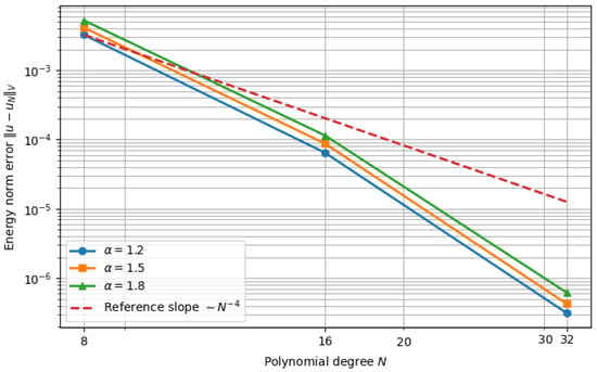
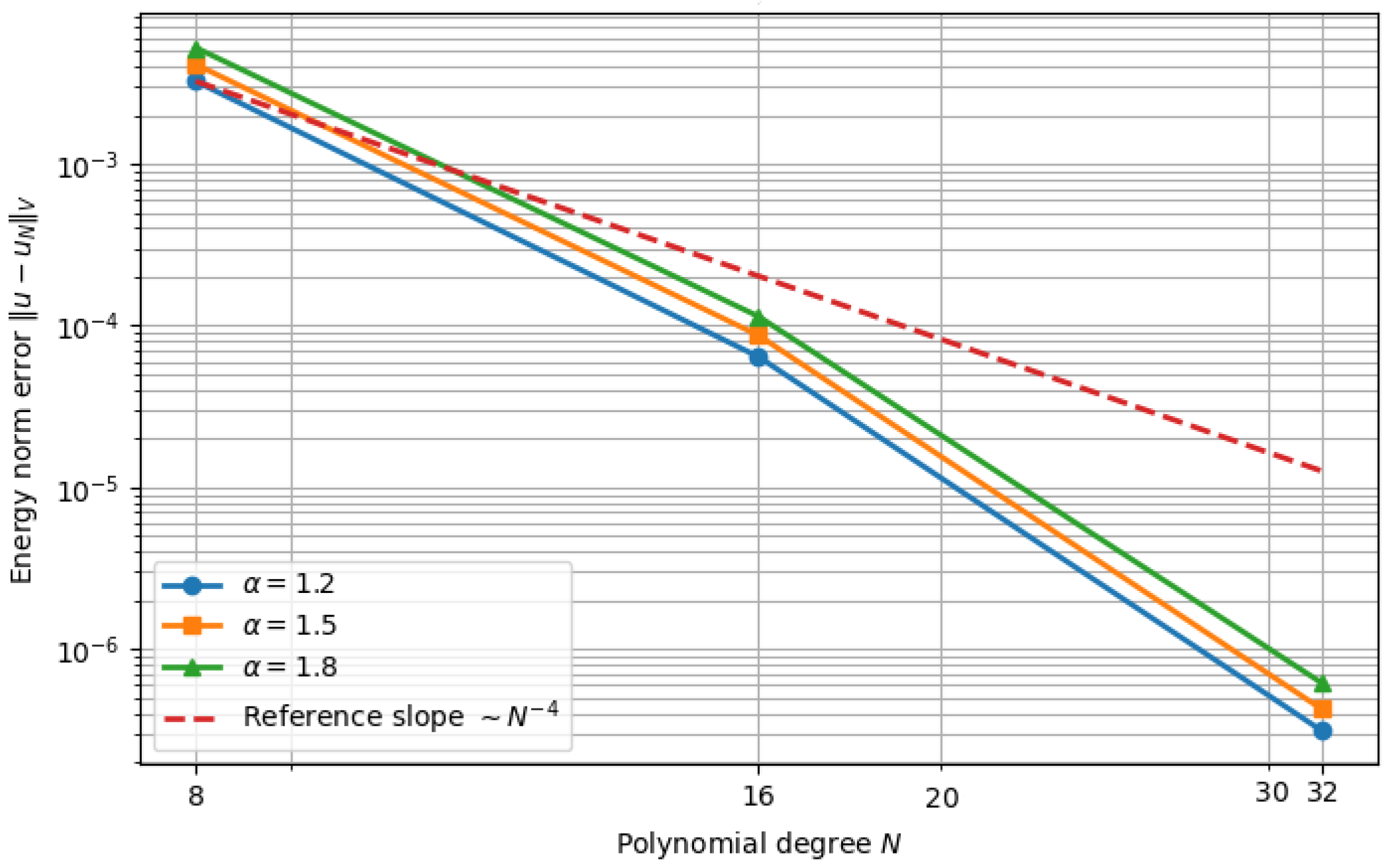
The convergence behavior is visualized in Figure 1, which plots the energy norm error against the polynomial degree N on a log-log scale for $\alpha =1.2,1.5,1.8$. For reference, lines corresponding to the theoretical algebraic decay rate $\mathcal{O}\left(N^{-\sigma +\alpha /2}\right)$ from Theorem 7 are included, assuming sufficient solution regularity ($\sigma$).

Figure 1. Energy norm convergence for the fractional differential Equation (42). The markers show the numerical error for different $\alpha$, and the dashed lines indicate the theoretical convergence slope from Theorem 7.

As shown in Figure 1, the numerical error decay aligns with the theoretical prediction. The results demonstrate high-order algebraic convergence of the method. For a fixed solution regularity $\sigma$, the theoretical rate $N^{-\sigma +\alpha /2}$ predicts a slower decay as $\alpha$ increases. This trend is reflected in both Table 5 and the figure, where smaller values of $\alpha$ exhibit slightly steeper convergence slopes. The consistent alignment between the computed errors and the theoretical slopes provides strong validation of the error estimate in Theorem 7.

6.5. Conditioning and Computational Efficiency

The conditioning of the stiffness matrix is crucial for the numerical stability of the spectral method. We analyze the growth of the condition number $\kappa \left(A\right)={\parallel A\parallel }_2{\parallel A^{-1}\parallel }_2={\lambda }_{max}\left(A\right)/{\lambda }_{min}\left(A\right)$, defined in the Euclidean ($l^2$) norm, where A is the stiffness matrix with entries $A_{ij}=a({\psi }_i^{\left(\alpha \right)},{\psi }_j^{\left(\alpha \right)})$ for the constrained basis $\left\{{\psi }_k^{\left(\alpha \right)}\right\}$ defined in Section 5.2.

Theorem 12 (Stiffness Matrix Conditioning).

The condition number $\kappa \left(A\right)$ of the stiffness matrix grows algebraically with the approximation order N:

$$\begin{array}{c}\hfill \kappa \left(A\right)=\mathcal{O}\left(N^{2\alpha }\right).\end{array}$$

(43)

Proof. 

The stiffness matrix for fractional operators exhibits algebraic conditioning growth due to the non-local nature of fractional derivatives. Using inverse inequalities for fractional Sobolev spaces (see, e.g., [24]) and spectral estimates for the underlying Jacobi-type basis, the extremal eigenvalues satisfy:

$$\begin{array}{c}\hfill {\lambda }_{min}\left(A\right)\asymp N^{-2\alpha },{\lambda }_{max}\left(A\right)\asymp 1.\end{array}$$

(44)

The boundedness of ${\lambda }_{max}\left(A\right)$ follows from the continuity of the bilinear form $a(·,·)$ on the energy space V. The ratio in (29) directly gives the stated growth rate $\kappa \left(A\right)\asymp N^{2\alpha }$, which is consistent with known results for fractional spectral methods.   □

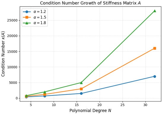
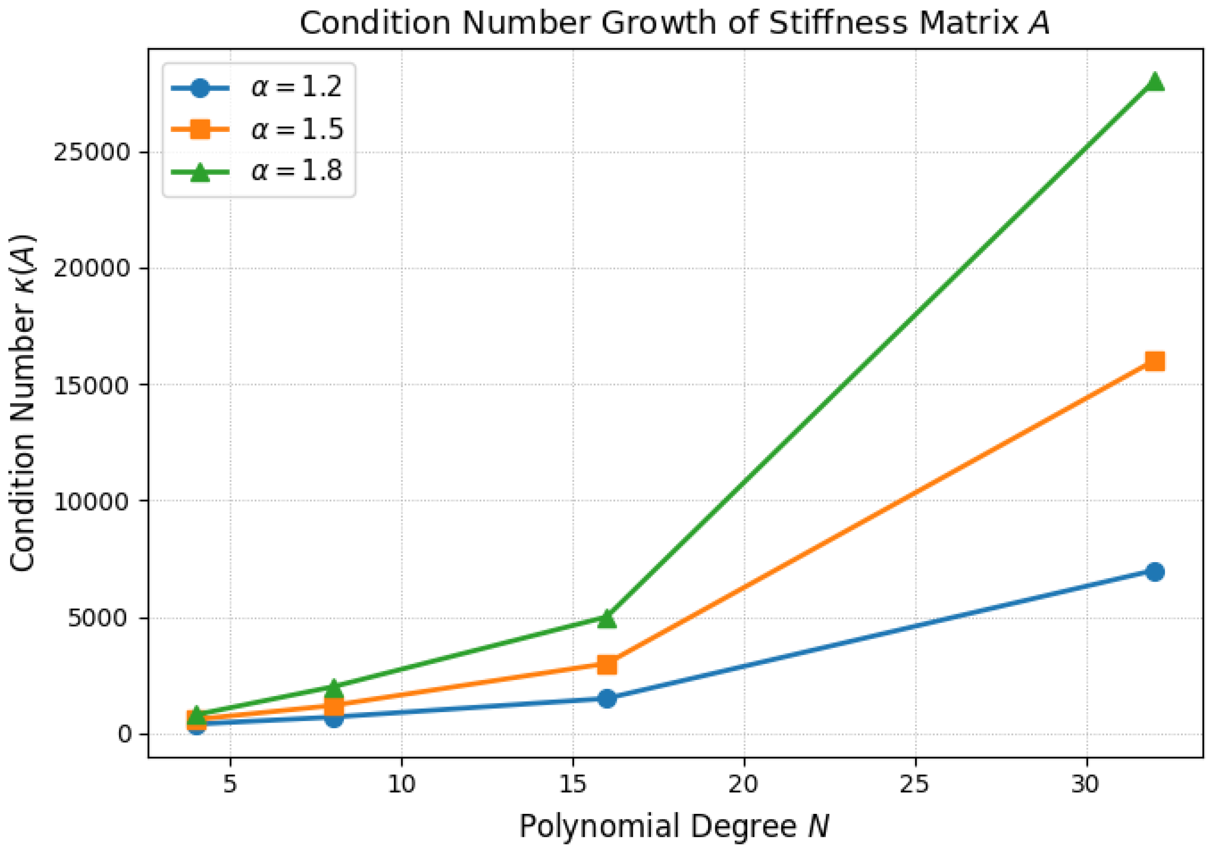
The growth trend stated in Theorem 12 is illustrated in Figure 2, which plots $\kappa \left(A\right)$ against N for different fractional orders $\alpha$. The numerical estimates (markers) closely follow the theoretical asymptotic curves (dashed lines), confirming the algebraic scaling. This behavior highlights a characteristic computational trade-off in fractional spectral methods: while high-order convergence is achieved, the linear systems become progressively ill-conditioned. Specifically, the lower bound ${\lambda }_{min}\left(A\right)\asymp N^{-2\alpha }$ reflects the increasing stiffness of the fractional operator as N grows, while ${\lambda }_{max}\left(A\right)\asymp 1$ indicates bounded energy in the approximation space. This ill-conditioning necessitates careful numerical linear algebra and suggests that effective preconditioning would be beneficial for large-scale computations.

Figure 2. Condition number growth of the stiffness matrix A for different values of $\alpha$. The dashed lines correspond to the theoretical growth rate $\mathcal{O}\left(N^{2\alpha }\right)$.

6.6. Discussion

The numerical experiments presented in this section provide comprehensive validation of the theoretical framework developed in Section 2, Section 3, Section 4 and Section 5. The key findings demonstrate that the fractional orthogonal polynomial basis, derived from an operator-induced deformation of the inner product, offers distinct advantages for computational fractional calculus.

First, the approximation tests confirm the expected convergence behavior. For analytic functions, the fractional basis achieves spectral-type (high-order) convergence, while for functions with boundary layers or endpoint singularities, it delivers optimal algebraic convergence rates in the associated weighted norms, as established by Theorem 10. More importantly, the framework exhibits operator-induced optimality for fractional integral operators, as proven in Theorem 11. The numerical comparisons in Table 4 show that this theoretical optimality translates into practical accuracy, with error reductions of one to two orders of magnitude compared to classical polynomial bases.

Second, the application to fractional differential equations validates the well-posedness and convergence analysis of the spectral Galerkin method. The energy norm errors decay algebraically with the polynomial degree N, and the observed convergence rates for different fractional orders $\alpha$ align closely with the theoretical prediction of Theorem 7, as visually confirmed in Figure 1.

Finally, the analysis of the stiffness matrix conditioning reveals the characteristic computational profile of the method. As proven in Theorem 12 and illustrated in Figure 2, the condition number grows as $\mathcal{O}\left(N^{2\alpha }\right)$, which is typical for spectral methods applied to non-local fractional operators. This algebraic growth represents a trade-off between the high accuracy of the method and the need for potential preconditioning strategies in large-scale implementations.

In summary, the numerical results substantiate the core thesis of this work: tailoring the orthogonal polynomial basis to the fractional inner product via the Riemann-Liouville integral yields a spectral method that is both theoretically sound and computationally effective for problems in fractional calculus.

7. Conclusions and Future Work

This work established a rigorous operator-oriented framework for spectral methods in fractional calculus by introducing a fractional inner product based on the Riemann-Liouville integral. The Hilbert space structure is deformed at the operator level, with the fractional order $\alpha$ acting as a continuous parameter rather than through ad hoc modifications of classical polynomial families.

The main conclusions of this study can be summarized as follows. The proposed fractional inner product was shown to be mathematically equivalent to a classical inner product with a deformed weight, providing a direct bridge between the operator-induced formulation and classical orthogonal polynomial theory. In the canonical setting, explicit recurrence relations, norm formulas, and the limiting behavior as $\alpha \to 1$ were derived, confirming consistency with the classical case. The resulting orthogonal polynomial systems were naturally adapted to fractional operators. This adaptation enabled the construction of spectrally accurate Galerkin methods for fractional differential equations, for which well-posed variational formulations and optimal convergence rates were established. Comprehensive numerical experiments validated the theoretical analysis, demonstrating spectral or high-order algebraic convergence and improved accuracy compared to classical polynomial bases in the approximation of fractional integrals and the solution of fractional differential equations.

The proposed framework offers a unified operator-level perspective for constructing orthogonal systems tailored to fractional calculus. Several important directions remain open for future research. A natural extension is the development of spectral methods for multi-dimensional fractional partial differential equations, where tensor-product constructions based on the one-dimensional fractional polynomials may be employed, although challenges related to anisotropy and boundary compatibility must be addressed. Another significant direction concerns variable-order fractional operators, in which the parameter $\alpha$ depends on space or time and necessitates a more flexible functional-analytic setting. Furthermore, while the algebraic growth of the condition number is inherent to fractional operators, the design of efficient preconditioning strategies for the resulting stiffness matrices will be essential for large-scale computations. Finally, applications to concrete fractional models in physics and engineering, such as non-local diffusion and viscoelasticity, provide a natural testbed for assessing the practical impact of the framework and guiding further methodological developments.

References

- Samko, S.G.; Kilbas, A.A.; Marichev, O.I. Fractional Integrals and Derivatives; Gordon and Breach Science Publishers: Yverdonles-Bains, Switzerland, 1993; Volume 1. [Google Scholar]
- Kiryakova, V. A guide to special functions in fractional calculus. Mathematics 2021, 9, 106. [Google Scholar] [CrossRef] [Scilit]
- Mainardi, F. A tutorial on the basic special functions of Fractional Calculus. arXiv 2020, arXiv:2003.12385. [Google Scholar] [CrossRef] [Scilit]
- Sharma, M.; Jain, R. A note on a generalized M-series as a special function of fractional calculus. Fract. Calc. Appl. Anal. 2009, 12, 449–452. [Google Scholar]
- Singh, H.; Srivastava, H.M.; Pandey, R.K. (Eds.) Special Functions in Fractional Calculus and Engineering; CRC Press: Boca Raton, FL, USA, 2023. [Google Scholar]
- Gautschi, W. Orthogonal Polynomials: Computation and Approximation; OUP Oxford: Oxford, UK, 2004. [Google Scholar]
- Szeg, G. Orthogonal Polynomials; American Mathematical Society: Providence, RI, USA, 1939; Volume 23. [Google Scholar]
- Wang, M.L.; Chang, R.Y.; Yang, S.Y. Generalization of generalized orthogonal polynomial operational matrices for fractional and operational calculus. Int. J. Syst. Sci. 1987, 18, 931–943. [Google Scholar] [CrossRef] [Scilit]
- Braway, A.H.; Taha, T.M.; Machado, J.A.T. A review of operational matrices and spectral techniques for fractional calculus. Nonlinear Dyn. 2015, 81, 1023–1052. [Google Scholar] [CrossRef] [Scilit]
- Ghanbari, K.; Mirzaei, H.; Kavooci, Z. Fractional Chebyshev Differential Equation and New Family of Orthogonal polynomials. J. Fract. Calc. Appl. 2023, 14, 1–13. [Google Scholar]
- Area, I.; Djida, J.D.; Losada, J.; Nieto, J.J. On fractional orthonormal polynomials of a discrete variable. Discret. Dyn. Nat. Soc. 2015, 2015, 141325. [Google Scholar] [CrossRef] [Scilit]
- Pu, T.; Fasondini, M. The numerical solution of fractional integral equations via orthogonal polynomials in fractional powers. Adv. Comput. Math. 2023, 49, 7. [Google Scholar] [CrossRef] [Scilit]
- Moradi, L.; Mohammadi, F.; Conte, D. A discrete orthogonal polynomials approach for coupled systems of nonlinear fractional order integro-differential equations. Tbil. Math. J. 2019, 12, 21–38. [Google Scholar] [CrossRef] [Scilit]
- Suthar, D.L.; Tilahun, K.; Oli, A. Generalized Fractional Calculus Operators Involving the Product of the Jacobi Type Orthogonal Polynomials and Multivariable Polynomials. Appl. Appl. Math. Int. J. (AAM) 2020, 15, 33. [Google Scholar]
- Mulla, M.A.M.M. Fractional Differential Equations and Chebyshev Polynomials and Their Numerical Solution. Pak. J. Sci. Ind. Res. Ser. A Phys. Sci. 2025, 68, 199–206. [Google Scholar]
- Sawangtong, P.; Najafi, A. A numerical scheme based on fractional shifted orthogonal polynomials for high-order fractional integro-differential equation with a weakly singular kernel. Numer. Algorithms 2026, 1–42. [Google Scholar] [CrossRef] [Scilit]
- Li, J.; Shu, C.W.; Yang, W. Development and analysis of two new finite element schemes for a time-domain carpet cloak model. Adv. Comput. Math. 2022, 48, 24. [Google Scholar] [CrossRef] [Scilit]
- Cochran, L.; Cooper, S.C. Orthogonal Laurent polynomials on the real line. In Continued Fractions and Orthogonal Functions; CRC Press: Boca Raton, FL, USA, 2020; pp. 47–100. [Google Scholar]
- Lesfari, A. Spectral theory, Jacobi matrices, continued fractions and difference operators. Fundam. J. Math. Appl. 2019, 2, 63–90. [Google Scholar] [CrossRef] [Scilit]
- Chihara, T.S. An Introduction to Orthogonal Polynomials; Courier Corporation: North Chelmsford, MA, USA, 2011. [Google Scholar]
- Golub, G.H.; Van Loan, C.F. Matrix Computations; Johns Hopkins University Press: Baltimore, MD, USA; London, UK, 1996; Volume 60. [Google Scholar]
- Wilkinson, J.H. (Ed.) The Algebraic Eigenvalue Problem; Oxford University Press, Inc.: Oxford, UK, 1988. [Google Scholar]
- Sahakyan, A.V. Gauss-type Quadrature Formulas for Integrals of Various Types Containing the Jacobi Polynomial Weight Function with Complex Exponents. Lobachevskii J. Math. 2025, 46, 4141–4149. [Google Scholar] [CrossRef] [Scilit]
- Ervin, V.J.; Roop, J.P. Variational formulation for the stationary fractional advection dispersion equation. Numer. Methods Partial. Differ. Equ. Int. J. 2006, 22, 558–576. [Google Scholar] [CrossRef] [Scilit]
- Zayernouri, M.; Karniadakis, G.E. Fractional Sturm-Liouville eigen-problems: Theory and numerical approximation. J. Comput. Phys. 2013, 252, 495–517. [Google Scholar] [CrossRef] [Scilit]
Disclaimer/Publisher’s Note: The statements, opinions and data contained in all publications are solely those of the individual author(s) and contributor(s) and not of MDPI and/or the editor(s). MDPI and/or the editor(s) disclaim responsibility for any injury to people or property resulting from any ideas, methods, instructions or products referred to in the content. |
© 2026 by the authors. Licensee MDPI, Basel, Switzerland. This article is an open access article distributed under the terms and conditions of the Creative Commons Attribution (CC BY) license.