Corrected L1 Scheme for the Fractional Subdiffusion Equation

Abstract

In this paper, a second-order implicit difference scheme for the time-fractional subdiffusion equation is constructed using a corrected L1 approximation of the fractional derivative. Estimates for the generating functions and resolvent coefficients are derived and used to establish the stability and convergence of the scheme. Numerical results are consistent with the theoretical error estimates and confirm the second-order accuracy of the scheme.

1. Introduction

Fractional differential equations (FDEs) have become an important tool for describing dynamical processes with memory and hereditary effects. In contrast to classical differential operators, fractional derivatives are nonlocal and therefore account for the entire history of the underlying process. Fractional models are particularly well suited to describing anomalous diffusion [1], heat conduction in heterogeneous media [2], viscoelastic behavior [3], transport in porous materials [4], fractional-order control systems [5], biological processes [6], and financial dynamics [7].

Among the commonly used fractional derivatives, the Caputo derivative is particularly well suited to initial-value problems because it allows initial conditions to be formulated in terms of integer-order derivatives. For $0<\alpha <1$, the Caputo fractional derivative is defined by

$$D_t^{\alpha }f\left(t\right)=f^{\left(\alpha \right)}\left(t\right)={\displaystyle \frac{1}{\Gamma (1-\alpha )}}{\int }_l^t{\displaystyle \frac{f^{\prime }\left(\tau \right)}{{(t-\tau )}^{\alpha }}}d\tau ,$$

where l is the lower terminal of fractional differentiation and $\Gamma (·)$ denotes the Gamma function. The weakly singular kernel in the definition of the Caputo fractional derivative accounts for the memory effect of the model and poses significant challenges for its numerical treatment. In particular, standard approximations of the fractional derivative involve the values of the function at all preceding time levels. Consequently, direct implementations of time-stepping schemes generally incur greater computational cost and storage requirements than classical schemes for partial differential equations with integer-order derivatives. Moreover, the kernel singularity and the limited temporal regularity of the solution can reduce the accuracy of standard time discretizations.

One of the most widely used approximations of the Caputo derivative is the L1 formula. Without loss of generality, we take the lower terminal of the fractional derivative to be zero. Let $t_n=n\tau$, where $\tau >0$ is a uniform time step, and let $f_n=f\left(t_n\right)$. The L1 approximation can be written as [8] (p. 140).

$$\begin{array}{c}\hfill {\displaystyle \frac{1}{\Gamma (2-\alpha ){\tau }^{\alpha }}}{\displaystyle \sum _{k=0}^n}{\sigma }_k^{\left(\alpha \right)}{f}_{n-k}=f_n^{\left(\alpha \right)}+\mathcal{O}\left({\tau }^{2-\alpha }\right),\hfill \\ \hfill {\sigma }_0^{\left(\alpha \right)}=1,{\sigma }_k^{\left(\alpha \right)}={(k-1)}^{1-\alpha } -2k^{1-\alpha }+{(k+1)}^{1-\alpha },1\le k<n,\hfill \end{array}$$

(1)

and has a terminal weight ${\sigma }_n^{\left(\alpha \right)}={(n-1)}^{1-\alpha }-n^{1-\alpha }$. When $f\in C^2[0,t_n]$, the L1 approximation has an accuracy of order $\mathcal{O}\left({\tau }^{2-\alpha }\right)$ and a generating function

$$S\left(z\right)={\displaystyle \sum _{k=0}^{\infty }}{\sigma }_k^{\left(\alpha \right)}{z}^k={(1-z)}^2{\displaystyle \frac{{\mathrm{Li}}_{\alpha -1}\left(z\right)}{z}},$$

where ${\mathrm{Li}}_s\left(z\right)$ denotes the polylogarithm. The simple convolution structure of the L1 formula, its robustness, and the favorable monotonicity properties of its coefficients have made it a standard choice for constructing finite difference schemes for time-fractional problems. A substantial body of literature addresses the development of L1-based schemes for fractional differential equations and the analysis of their stability and convergence on uniform and graded meshes [9,10,11,12]. A comprehensive recent survey of the L1 method and its variants, including weighted, averaged, and fast versions, is provided in [13], where the flexibility and limitations of classical L1-based discretizations are discussed in detail. The development of higher-order approximations remains an active area of research. Notable examples include Lubich’s convolution quadrature [14,15], the L1-2 formula of Gao, Sun, and Zhang [16], and the L2-$1_{\sigma }$ formula introduced by Alikhanov [17]. A new L2-type difference scheme (NL2) was recently proposed in [18], where a piecewise quadratic polynomial interpolation is used to approximate the Caputo derivative, achieving $(3-\alpha )$-th order accuracy and $H^1$-norm stability on uniform meshes. Starting corrections have also been developed to restore higher-order convergence in the presence of initial singularities [19,20]. More recently, convolution quadrature based on block generalized Adams methods has been developed for subdiffusion equations, achieving high-order convergence on uniform grids through the inclusion of correction terms [21]. Although these methods offer improved accuracy, their analysis can be more involved, and certain formulations require shifted evaluation points, additional starting procedures, or stronger regularity assumptions. These considerations motivate the development of modifications of the L1 formula that retain its simple convolution structure while achieving higher-order accuracy. A second-order corrected L1 approximation whose weights retain the monotonicity properties of the original L1 formula was constructed in [22] and used to develop a finite difference scheme for the time-fractional subdiffusion equation (TFSE). These properties facilitate the analysis of the unconditional stability and convergence of the scheme. Various modifications of the L1 formula have been proposed to improve its accuracy, stability properties, and computational efficiency. Examples include the corrected L1 method [23], the fitted L1 method [24], and the weighted L1 method [13]. Alternative correction strategies for the L1 weights have also been explored in [23], where a corrected L1 method achieving second-order accuracy for subdiffusion problems was developed and analyzed. The averaged L1 scheme, which combines adjacent L1 weights to improve accuracy while maintaining simplicity, has been rigorously analyzed for subdiffusion problems in [25], where second-order convergence was established under appropriate regularity assumptions. Higher-order methods on fitted meshes have also been developed for time-fractional diffusion problems with nonsmooth solutions, where the singularity of the solution at the initial time is treated by a suitable mesh grading [26]. Error analysis of the L1 method on graded and uniform meshes has been extended to two- and three-dimensional fractional-derivative problems in [27], providing sharp convergence estimates in higher spatial dimensions. The corrected L1 approximation of the fractional derivative constructed in [22] has an accuracy $\mathcal{O}({\tau }^{2-\alpha }/n^{\alpha })$, and uses a correction strategy that differs from that of the corrected L1 method in [23]. The proposed approximation has several distinctive features. Its weights retain the monotonicity properties of the classical L1 approximation, facilitating the stability analysis of numerical schemes for fractional differential equations. Moreover, although the approximation has an order of accuracy below two, the resulting numerical solutions achieve second-order accuracy [22].

In a recent study [28], the following corrected L1 approximation was derived and used to develop numerical schemes for fractional ordinary differential equations.

$$\begin{array}{cc}\hfill {\displaystyle \frac{1}{\Gamma (2-\alpha ){\tau }^{\alpha }}}{\displaystyle \sum _{k=0}^n}& {\gamma }_k^{\left(\alpha \right)}{f}_{n-k}=f_n^{\left(\alpha \right)}+\mathcal{O}\left({\displaystyle \frac{{\tau }^{2-\alpha }}{n^{\alpha }}}\right),\hfill \\ \hfill {\gamma }_0^{\left(\alpha \right)}=1-\zeta (\alpha -1),{\gamma }_1^{\left(\alpha \right)}=2^{1-\alpha }-& 2+2\zeta (\alpha -1),{\gamma }_2^{\left(\alpha \right)}=3^{1-\alpha }-2^{2-\alpha }+1-\zeta (\alpha -1),\hfill \\ \hfill {\gamma }_k^{\left(\alpha \right)}={\sigma }_k^{\left(\alpha \right)}={(k-1)}^{1-\alpha }-2k^{1-\alpha }+& {(k+1)}^{1-\alpha },{\gamma }_n^{\left(\alpha \right)}={\sigma }_n^{\left(\alpha \right)}={(n-1)}^{1-\alpha }-n^{1-\alpha },\hfill \end{array}$$

(2)

where $2<k<n$. Corrected L1 approximation (2) has a generating function

$$G\left(z\right)={\displaystyle \sum _{k=0}^{\infty }}{\gamma }_k^{\left(\alpha \right)}{z}^k={(1-z)}^2\left({\displaystyle \frac{{\mathrm{Li}}_{\alpha -1}\left(z\right)}{z}}-\zeta (\alpha -1)\right).$$

Approximation (2) is obtained from the L1 formula by applying a correction to its first three weights based on the central difference formula and the value $\zeta (\alpha -1)$ of the Riemann zeta function. This correction cancels the leading term in the asymptotic expansion of the L1 error, yielding an error of order $\mathcal{O}\left({\tau }^{2-\alpha }{n}^{-\alpha }\right)$. The corrected approximation (2) also extends to fractional derivatives of order $\alpha$, with $1<\alpha <2$, by incorporating a correction term involving the first derivative of the function at the lower terminal. In [28], we proved that numerical schemes for fractional ordinary differential equations based on this approximation achieve second-order accuracy. In the present paper, we extend this approach to the TFSE by constructing a second-order implicit finite difference scheme. We establish the stability and convergence of the scheme using properties of its generating function and the associated resolvent coefficients.

The numerical solution of fractional diffusion equations has received considerable attention because these equations provide effective mathematical models for transport processes with memory and temporal nonlocality. Anomalous diffusion occurs in many natural and engineering systems, including contaminant transport through porous media, drug dispersion in biological tissues, and asset-price dynamics in financial models. Classical diffusion models are based on Brownian motion, in which the mean-square displacement is proportional to time. However, numerous experimental studies have shown that many real-world transport processes deviate from this behavior and instead display subdiffusive or superdiffusive dynamics. FDEs provide an effective mathematical framework for modeling such phenomena, since their nonlocal structure, memory effects, and hereditary properties naturally capture the long-range correlations present in complex systems. The nonlocality of fractional derivatives poses computational challenges, as numerical approximations typically require information from the entire preceding evolution of the solution. These challenges motivate the development of accurate and stable numerical methods that account for memory effects while maintaining a manageable computational cost.

Finite difference schemes are widely used for time-fractional differential equations because they provide simple and efficient discretizations of the nonlocal fractional derivative while retaining a familiar structure for the spatial operators. The theoretical analysis of these schemes typically focuses on consistency, stability, solvability, and convergence. Common tools for stability and convergence analysis include discrete energy estimates, eigenfunction expansions and matrix analysis, generating-function techniques, discrete fractional Grönwall inequalities, and estimates for discrete convolution kernels. Generating-function methods are particularly useful for schemes with corrected convolution weights, as they allow one to investigate the positivity of the real part on the unit circle and its asymptotic behavior near $z=1$. These properties provide a basis for estimating the associated resolvent coefficients and establishing stability and convergence. Many numerical methods originally developed for classical differential equations have been adapted and extended to the solution of fractional differential equations. Fractional linear multistep methods provide a systematic framework for the numerical solution of TFSE by approximating the fractional derivative through discrete convolution operators generated from classical linear multistep methods [14,15]. Weighted and shifted Grünwald–Letnikov formulas offer another effective approach, allowing the construction of higher-order time-stepping schemes and, with suitable starting corrections, retaining high accuracy even for solutions with limited regularity near the initial time [29]. Fast schemes based on sum-of-exponentials approximations of the weakly singular kernel have been developed to reduce the computational cost and memory requirements associated with the history term in fractional diffusion problems [30,31]. All-at-once implementations on time nonuniform meshes have also been developed for subdiffusion equations, where the entire space–time system is solved simultaneously and geometric time-step grading is employed to handle the initial singularity efficiently [32]. Hybrid numerical approaches combining the L1 scheme with multi-dimensional Hermite wavelets have been developed for time-fractional sub-diffusion equations with multi-singularities on newly designed time-graded meshes, achieving robust accuracy with reduced computational cost [33]. Spectral-in-time methods approximate the temporal solution by global polynomial basis functions and can achieve very high-order or spectral convergence when the solution possesses sufficient temporal regularity [34]. Space–time spectral and finite difference–spectral methods have also been developed for fractional diffusion equations, providing accurate alternatives to conventional finite-difference discretizations, particularly for smooth solutions [9,34].

A central goal in the design of numerical methods for fractional diffusion equations is to achieve high-order accuracy and unconditional stability while maintaining a simple structure and moderate computational cost. Corrected L1 schemes offer a promising approach, as they retain the convolution structure of the classical L1 method while improving its temporal accuracy. In this paper, we construct and analyze an implicit finite difference scheme based on approximation (2) for the time-fractional subdiffusion problem. A key difficulty is that the correction modifies the first three weights of the L1 formula, preventing a direct application of the standard stability arguments based on the signs and monotonicity of the classical L1 weights. We overcome this difficulty by analyzing the generating function of the corrected L1 approximation (2) and the associated resolvent coefficients.

The paper is organized as follows. Section 2 studies the generating function of the corrected L1 formula, including its integral representation, positivity, and the estimates required for the resolvent analysis. Section 3 introduces the corrected L1 finite difference scheme for the time-fractional subdiffusion equation, derives bounds for the discrete resolvent coefficients, and establishes the stability and second-order convergence of the implicit difference scheme. The numerical experiments confirm the theoretical error estimates and convergence order of the implicit difference scheme for the TFSE.

2. Properties of the Generating Functions

Let ${\beta }_k^{\left(\alpha \right)}$ be the first-order difference sequence of the L1 approximation

$${\beta }_k^{\left(\alpha \right)}={(k+1)}^{1-\alpha }-k^{1-\alpha },$$

for $k\ge 0$. The L1 coefficients satisfy

$${\sigma }_0^{\left(\alpha \right)}={\beta }_0^{\left(\alpha \right)}=1,{\sigma }_k^{\left(\alpha \right)}={\beta }_k^{\left(\alpha \right)}-{\beta }_{k-1}^{\left(\alpha \right)},k\ge 1,$$

and the sequence ${\beta }_k^{\left(\alpha \right)}$ has a generating function

$$B\left(z\right)={\displaystyle \sum _{k=0}^{\infty }}{\beta }_k^{\left(\alpha \right)}{z}^k={\displaystyle \frac{S\left(z\right)}{1-z}}={\displaystyle \frac{(1-z){\mathrm{Li}}_{\alpha -1}\left(z\right)}{z}}.$$

Next, we derive an integral representation for the function $B\left(x\right)$.

Lemma 1. 

For $\left|z\right|<1$,

$$B\left(z\right)={\displaystyle \frac{1-\alpha }{\Gamma \left(\alpha \right)}}{\int }_0^{\infty }{t}^{\alpha -2}{\displaystyle \frac{1-e^{-t}}{1-e^{-t}z}}dt.$$

Proof. 

The numbers ${\beta }_k^{\left(\alpha \right)}$ satisfy

$${\beta }_k^{\left(\alpha \right)}={(k+1)}^{1-\alpha }-k^{1-\alpha }=(1-\alpha ){\int }_0^1{(k+s)}^{-\alpha }ds.$$

For $x>0$ and $u=xt$,

$$\begin{array}{cc}\hfill {\int }_0^{\infty }{t}^{\alpha -1}{e}^{-xt}dt={\int }_0^{\infty }& {\left({\displaystyle \frac{u}{x}}\right)}^{\alpha -1}{e}^{-u}{\displaystyle \frac{du}{x}}={\displaystyle \frac{1}{x^{\alpha }}}{\int }_0^{\infty }{u}^{\alpha -1}{e}^{-u}du={\displaystyle \frac{\Gamma \left(\alpha \right)}{x^{\alpha }}}.\hfill \end{array}$$

Hence,

$$x^{-\alpha }={\displaystyle \frac{1}{\Gamma \left(\alpha \right)}}{\int }_0^{\infty }{t}^{\alpha -1}{e}^{-xt}dt,$$

and

$$\begin{array}{cc}\hfill {\beta }_k^{\left(\alpha \right)}& ={\displaystyle \frac{1-\alpha }{\Gamma \left(\alpha \right)}}{\int }_0^{\infty }{t}^{\alpha -1}{e}^{-kt}\left({\int }_0^1{e}^{-st}ds\right)dt={\displaystyle \frac{1-\alpha }{\Gamma \left(\alpha \right)}}{\int }_0^{\infty }{t}^{\alpha -2}\left(1-e^{-t}\right)e^{-kt}dt.\hfill \end{array}$$

For $\left|z\right|<1$,

$$B\left(z\right)={\displaystyle \sum _{k=0}^{\infty }}{\beta }_k^{\left(\alpha \right)}{z}^k={\displaystyle \frac{1-\alpha }{\Gamma \left(\alpha \right)}}{\int }_0^{\infty }{t}^{\alpha -2}(1-e^{-t}){\displaystyle \sum _{k=0}^{\infty }}{\left(e^{-t}z\right)}^{k}dt.$$

Summing the geometric series gives

$$B\left(z\right)={\displaystyle \frac{1-\alpha }{\Gamma \left(\alpha \right)}}{\int }_0^{\infty }{\displaystyle \frac{t^{\alpha -2}(1-e^{-t})}{1-e^{-t}z}}dt.$$

□

2.1. Real Part of the Generating Function

By Lemma 1 the generating function of the L1 approximation (1) has an integral representation

$$S\left(z\right)=(1-z)B\left(z\right)={\displaystyle \frac{1-\alpha }{\Gamma \left(\alpha \right)}}{\int }_0^{\infty }{t}^{\alpha -2}{\displaystyle \frac{(1-e^{-t})(1-z)}{1-e^{-t}z}}dt$$

(3)

and

$$G\left(z\right)=S\left(z\right)-{(1-z)}^2\zeta (\alpha -1)$$

is the generating function of the corrected L1 formula. Let

$$z=e^{i\theta },x=\mathrm{Re}\left(z\right)=\cos \theta ,r=e^{-t}.$$

Lemma 2. 

$$\mathrm{Re}\left(G\left(e^{i\theta }\right)\right)=(1-x)\left(J_{\alpha }\left(x\right)+2\zeta (\alpha -1)x\right).$$

(4)

where

$$J_{\alpha }\left(x\right)={\displaystyle \frac{1-\alpha }{\Gamma \left(\alpha \right)}}{\int }_0^{\infty }{t}^{\alpha -2}{\displaystyle \frac{1-e^{-2t}}{1-2e^{-t}x+e^{-2t}}}dt.$$

(5)

Proof. 

Let r be a real number. Then

$$\mathrm{Re}\left({\displaystyle \frac{1-z}{1-rz}}\right)=\mathrm{Re}\left({\displaystyle \frac{(1-z)(1-r\overline{z})}{(1-rz)(1-r\overline{z})}}\right)=\mathrm{Re}\left({\displaystyle \frac{1-z-r\overline{z}+r{\left|z\right|}^2}{1-rz-r\overline{z}+r^2{\left|z\right|}^2}}\right).$$

The denominator is real. Therefore

$$\mathrm{Re}\left({\displaystyle \frac{1-z}{1-rz}}\right)={\displaystyle \frac{1-x-rx+r}{1-2rx+r^2}}={\displaystyle \frac{(1+r)(1-x)}{1-2rx+r^2}}.$$

(6)

By (3), (6), and  $r=e^{-t}$,

$$\mathrm{Re}\left(S\left(e^{i\theta }\right)\right)={\displaystyle \frac{1-\alpha }{\Gamma \left(\alpha \right)}}(1-x){\int }_0^{\infty }{t}^{\alpha -2}{\displaystyle \frac{1-e^{-2t}}{1-2e^{-t}x+e^{-2t}}}dt.$$

Also,

$$\begin{array}{cc}\hfill \mathrm{Re}\left({(1-z)}^2\right)=\mathrm{Re}\left({(1-e^{i\theta })}^2\right)& =1-2\cos \theta +\cos 2\theta \hfill \\ \hfill & =2{\cos }^2\theta -2\cos \theta =-2x(1-x).\hfill \end{array}$$

Therefore,

$$\begin{array}{cc}\hfill \mathrm{Re}\left(G\left(e^{i\theta }\right)\right)& =\mathrm{Re}\left(S\left(e^{i\theta }\right)\right)-\zeta (\alpha -1)\mathrm{Re}\left({(1-e^{i\theta })}^2\right)\hfill \\ \hfill & =(1-x)\left(J_{\alpha }\left(x\right)+2\zeta (\alpha -1)x\right).\hfill \end{array}$$

□

We next prove that the right-hand side of (4) is nonnegative. The proof relies on the following Mellin transform identity for the hyperbolic secant function.

Lemma 3. 

For every α with $\mathrm{Re}\left(\alpha \right)>0$,

$${\int }_0^{\infty }{t}^{\alpha -1}{\mathrm{sech}}^{2}tdt=2^{2-\alpha }\left(1-2^{2-\alpha }\right)\Gamma \left(\alpha \right)\zeta (\alpha -1).$$

(7)

Proof. 

For $t>0$, the hyperbolic tangent has the exponential series expansion

$$\begin{array}{c}\hfill \tanh t={\displaystyle \frac{e^t-e^{-t}}{e^t+e^{-t}}}=1-{\displaystyle \frac{2e^{-2t}}{1+e^{-2t}}}=1+2{\displaystyle \sum _{m=1}^{\infty }}{(-1)}^m{e}^{-2mt}.\end{array}$$

For every $\delta >0$ and $t\in [\delta ,\infty )$,

$$\left|2{(-1)}^m{e}^{-2mt}\right|\le 2e^{-2m\delta },\left|{\displaystyle \frac{d}{dt}}\left(2{(-1)}^m{e}^{-2mt}\right)\right|\le 4m{e}^{-2m\delta }.$$

Since

$${\displaystyle \sum _{m=1}^{\infty }}{e}^{-2m\delta }<\infty ,{\displaystyle \sum _{m=1}^{\infty }}m{e}^{-2m\delta }<\infty ,$$

the Weierstrass M-test shows that both the original series and the series of derivatives converge uniformly on $[\delta ,\infty )$. The theorem on termwise differentiation of uniformly convergent series [35] therefore gives

$${\mathrm{sech}}^{2}t={\displaystyle \frac{d}{dt}}\tanh t=4{\displaystyle \sum _{m=1}^{\infty }}{(-1)}^{m-1}m{e}^{-2mt}.$$

(8)

Substituting the series representation (8) into the left-hand side of (7) gives

$${\int }_0^{\infty }{t}^{\alpha -1}{\mathrm{sech}}^{2}tdt=4{\int }_0^{\infty }\left({\displaystyle \sum _{m=1}^{\infty }}{(-1)}^{m-1}m{t}^{\alpha -1}{e}^{-2mt}\right)dt.$$

Let $\omega =\mathrm{Re}\left(\alpha \right)$. We first evaluate the integral in the half-plane $\omega >2$. In this region, absolute integrability follows from

$$\begin{array}{cc}\hfill & {\displaystyle \sum _{m=1}^{\infty }}{\int }_0^{\infty }\left|4{(-1)}^{m-1}m{t}^{\alpha -1}{e}^{-2mt}\right|dt\hfill \\ \hfill & =4{\displaystyle \sum _{m=1}^{\infty }}m{\int }_0^{\infty }{t}^{\omega -1}{e}^{-2mt}dt=2^{2-\omega }\Gamma \left(\omega \right){\displaystyle \sum _{m=1}^{\infty }}{\displaystyle \frac{1}{m^{\omega -1}}}<\infty .\hfill \end{array}$$

Consequently, interchanging the sum and the integral is justified by Fubini’s theorem [36]. Therefore for $\mathrm{Re}\left(\alpha \right)>2$

$$\begin{array}{cc}\hfill {\int }_0^{\infty }{t}^{\alpha -1}{\mathrm{sech}}^{2}tdt& =4{\displaystyle \sum _{m=1}^{\infty }}{(-1)}^{m-1}m{\int }_0^{\infty }{t}^{\alpha -1}{e}^{-2mt}dt\hfill \\ \hfill & =4\Gamma \left(\alpha \right){\displaystyle \sum _{m=1}^{\infty }}{(-1)}^{m-1}{\displaystyle \frac{m}{{\left(2m\right)}^{\alpha }}}=2^{2-\alpha }\Gamma \left(\alpha \right){\displaystyle \sum _{m=1}^{\infty }}{(-1)}^{m-1}{\displaystyle \frac{1}{m^{\alpha -1}}},\hfill \end{array}$$

and

$${\int }_0^{\infty }{t}^{\alpha -1}{\mathrm{sech}}^{2}tdt=2^{2-\alpha }\Gamma \left(\alpha \right)\eta (\alpha -1).$$

(9)

In the half-plane $\mathrm{Re}\left(\alpha \right)>2$, the Dirichlet eta function satisfies

$$\eta (\alpha -1)={\displaystyle \sum _{m=1}^{\infty }}{\displaystyle \frac{{(-1)}^{m-1}}{m^{\alpha -1}}}.$$

The above series is absolutely convergent. Thus

$$\begin{array}{cc}\hfill \eta \left(\alpha -1\right)& ={\displaystyle \sum _{m=1}^{\infty }}{\displaystyle \frac{1}{m^{\alpha -1}}}-2{\displaystyle \sum _{m=1}^{\infty }}{\displaystyle \frac{1}{{\left(2m\right)}^{\alpha -1}}}=\left(1-2^{2-\alpha }\right)\zeta (\alpha -1),\hfill \end{array}$$

which proves (7) in half-plane $\mathrm{Re}\left(\alpha \right)>2$. We now extend (7) to the half-plane

$$\mathcal{P}=\{\alpha \in \mathbb{C}:\mathrm{Re}(\alpha )>0\}.$$

Define

$$F\left(\alpha \right)={\int }_0^{\infty }{t}^{\alpha -1}{\mathrm{sech}}^{2}tdt,\alpha \in \mathcal{P}.$$

For each fixed $t>0$, the integrand is an entire function of $\alpha$, because

$$t^{\alpha -1}=\exp \left((\alpha -1)\log t\right)$$

and $\log t$ is real. Let $K\subset \mathcal{P}$ be compact, and set

$${\omega }_0=\underset{\alpha \in K}{\min }\mathrm{Re}\left(\alpha \right)>0,{\omega }_1=\underset{\alpha \in K}{\max }\mathrm{Re}\left(\alpha \right).$$

For $0<t\le 1$ and $\alpha \in K$ the inequality

$${\mathrm{sech}}^{2}t={\displaystyle \frac{4e^{-2t}}{{(1+e^{-2t})}^2}}\le 1$$

gives

$$\left|t^{\alpha -1}{\mathrm{sech}}^{2}t\right|\le t^{{\omega }_0-1}.$$

For $t\ge 1$, we have

$${\mathrm{sech}}^{2}t={\displaystyle \frac{4e^{-2t}}{{(1+e^{-2t})}^2}}\le 4e^{-2t},$$

$$\left|t^{\alpha -1}{\mathrm{sech}}^{2}t\right|\le 4t^{{\omega }_1-1}{e}^{-2t}.$$

Both functions $t^{{\omega }_0-1}$ and $4t^{{\omega }_1-1}{e}^{-2t}$ are integrable on their respective intervals. Hence the integral defining F converges absolutely in the half-plane $\alpha \in \mathcal{P}$. By the theorem on holomorphic parameter integrals (see [35]), the function F is holomorphic on $\mathcal{P}$.

The zeta function $\zeta (\alpha -1)$ has a simple pole at $\alpha =2$, while the function $1-2^{2-\alpha }$ has a simple zero. Writing $\alpha =2+\epsilon$, we have

$$1-2^{2-\alpha }=\epsilon \log 2+\mathcal{O}\left({\epsilon }^2\right),\zeta (\alpha -1)={\displaystyle \frac{1}{\epsilon }}+\mathcal{O}\left(1\right).$$

Therefore,

$$\underset{\alpha \to 2}{\lim }\left(1-2^{2-\alpha }\right)\zeta (\alpha -1)=\log 2.$$

The singularity of $\left(1-2^{2-\alpha }\right)\zeta (\alpha -1)$ is removable, and at $\alpha =2$ the value of the right-hand side of (7) is $2^0\Gamma \left(2\right)\log 2=\log 2$. Next, define

$$H\left(\alpha \right)=2^{2-\alpha }\Gamma \left(\alpha \right)\eta (\alpha -1).$$

The relation

$$\eta \left(\alpha -1\right)=\left(1-2^{2-\alpha }\right)\zeta \left(\alpha -1\right),$$

initially obtained for $\mathrm{Re}\left(\alpha \right)>2$, provides the entire continuation of $\eta$ to the half-plane $\mathcal{P}$. Since $2^{2-\alpha }$ is entire and $\Gamma \left(\alpha \right)$ has no poles in $\mathcal{P}$, the function H is holomorphic in $\mathcal{P}$.

From (9), the holomorphic functions F and H agree on the nonempty open subset

$$\{\alpha \in \mathbb{C}:\mathrm{Re}(\alpha )>2\}\subset \mathcal{P}.$$

Since $\mathcal{P}$ is connected and $F=H$ on the open subset $\{\alpha \in \mathbb{C}:\mathrm{Re}(\alpha )>2\}\subset \mathcal{P},$ the identity theorem for holomorphic functions [35] implies that $F=H$ throughout $\mathcal{P}.$ □

Lemma 4. 

For $0<\alpha <1$ and $-\pi \le \theta \le \pi$,

$$\mathrm{Re}\left(G\left(e^{i\theta }\right)\right)\ge 0.$$

(10)

The inequality is strict for $\theta \ne 0$.

Proof. 

When $-1\le x\le 0$, the integrand in (5) is positive. Hence

$$J_{\alpha }\left(x\right)>0.$$

Since $\zeta (\alpha -1)<0$ and $x<0,$ we have $2\zeta (\alpha -1)x\ge 0.$ Therefore,

$$J_{\alpha }\left(x\right)+2\zeta (\alpha -1)x>0.$$

Because $1-x>0,$ Equation (4) gives $\mathrm{Re}\left(G\left(e^{i\theta }\right)\right)>0.$

Let $0<x<1$. For every fixed $t>0$, the denominator $1-2e^{-t}x+e^{-2t}$ decreases as x increases. Consequently,

$$J_{\alpha }\left(x\right)\ge J_{\alpha }\left(0\right).$$

At $x=0$,

$$\begin{array}{cc}\hfill J_{\alpha }\left(0\right)& ={\displaystyle \frac{1-\alpha }{\Gamma \left(\alpha \right)}}{\int }_0^{\infty }{t}^{\alpha -2}{\displaystyle \frac{1-e^{-2t}}{1+e^{-2t}}}dt={\displaystyle \frac{1-\alpha }{\Gamma \left(\alpha \right)}}{\int }_0^{\infty }{t}^{\alpha -2}\tanh tdt.\hfill \end{array}$$

Integrating by parts, using ${\displaystyle \frac{d}{dt}}\tanh t={\mathrm{sech}}^{2}t,$ and the facts

$$\underset{t\to 0^{+}}{\lim }{t}^{\alpha -1}\tanh t=0,\underset{t\to \infty }{\lim }{t}^{\alpha -1}\tanh t=0$$

gives

$$J_{\alpha }\left(0\right)={\displaystyle \frac{1-\alpha }{\Gamma \left(\alpha \right)}}\left({\left[{\displaystyle \frac{t^{\alpha -1}}{\alpha -1}}\tanh t\right]}_0^{\infty }-{\displaystyle \frac{1}{\alpha -1}}{\int }_0^{\infty }{t}^{\alpha -1}{\mathrm{sech}}^{2}tdt\right),$$

$$J_{\alpha }\left(0\right)={\displaystyle \frac{1}{\Gamma \left(\alpha \right)}}{\int }_0^{\infty }{t}^{\alpha -1}{\mathrm{sech}}^{2}tdt.$$

By Lemma 3

$$J_{\alpha }\left(0\right)=-2^{2-\alpha }\left(2^{2-\alpha }-1\right)\zeta (\alpha -1).$$

When $0<\alpha <1$, we have $2^{2-\alpha }\ge 2$, and therefore

$$J_{\alpha }\left(0\right)\ge -2\zeta (\alpha -1).$$

Consequently,

$$J_{\alpha }\left(x\right)\ge J_{\alpha }\left(0\right)>-2\zeta (\alpha -1)>-2\zeta (\alpha -1)x.$$

By Lemma 2

$$\mathrm{Re}\left(G\left(e^{i\theta }\right)\right)=(1-x)\left(J_{\alpha }\left(x\right)+2\zeta (\alpha -1)x\right)>0.$$

Finally, at $\theta =0$, we have $x=1$, and the factor $1-x$ vanishes. Hence $\mathrm{Re}\left(G\right(1\left)\right)=0.$ □

2.2. Estimates for the Generating Function

For $\left|\mu \right|<2\pi$, the polylogarithm has an expansion:

$${\mathrm{Li}}_s\left(e^{\mu }\right)=\Gamma (1-s){(-\mu )}^{s-1}+{\displaystyle \sum _{k=0}^{\infty }}\zeta (s-k){\displaystyle \frac{{\mu }^k}{k!}}.$$

(11)

Lemma 5. 

There exist positive constants $C_1,C_2$, independent of θ, such that

$$|G\left(e^{i\theta }\right)|\ge C_1{\left|\theta \right|}^{\alpha },-\pi \le \theta \le \pi ,$$

(12)

and

$$\left|{\displaystyle \frac{d}{d\theta }}G\left(e^{i\theta }\right)\right|\le C_2{\left|\theta \right|}^{\alpha -1},0<\left|\theta \right|\le \pi .$$

(13)

Proof. 

We first study the behavior of the generating function near $\theta =0$. From (11) with $s=\alpha -1$ and $\mu =i\theta ,$ we obtain

$${\mathrm{Li}}_{\alpha -1}\left(e^{i\theta }\right)=\Gamma (2-\alpha ){(-i\theta )}^{\alpha -2}+\zeta (\alpha -1)+i\zeta (\alpha -2)\theta +O\left({\theta }^2\right).$$

Also $e^{-i\theta }=1+O\left(\theta \right)$ and $1-e^{i\theta }=-i\theta +O\left({\theta }^2\right)$. Therefore

$$e^{-i\theta }{\mathrm{Li}}_{\alpha -1}\left(e^{i\theta }\right)-\zeta (\alpha -1)=\Gamma (2-\alpha ){(-i\theta )}^{\alpha -2}\left(1+o\left(1\right)\right).$$

Hence

$$\begin{array}{cc}\hfill G\left(e^{i\theta }\right)& ={(1-e^{i\theta })}^2\left(e^{-i\theta }{\mathrm{Li}}_{\alpha -1}\left(e^{i\theta }\right)-\zeta (\alpha -1)\right)\hfill \\ & =\Gamma (2-\alpha ){(-i\theta )}^{\alpha }(1+o\left(1\right)).\hfill \end{array}$$

Taking absolute values,

$$\underset{\theta \to 0}{\lim }{\displaystyle \frac{|G\left(e^{i\theta }\right)|}{{\left|\theta \right|}^{\alpha }}}=\Gamma (2-\alpha ).$$

Since $\Gamma (2-\alpha )>0$, there exists ${\delta }_1>0$ such that when $0<\left|\theta \right|\le {\delta }_1$,

$$\left|G\left(e^{i\theta }\right)\right|\ge {\displaystyle \frac{1}{2}}\Gamma (2-\alpha ){\left|\theta \right|}^{\alpha }.$$

(14)

The lower bound is now extended away from zero. By Lemma 4

$$\mathrm{Re}\left(G\left(e^{i\theta }\right)\right)>0,(\theta \ne 0).$$

Therefore $G\left(e^{i\theta }\right)\ne 0$ for $0<\left|\theta \right|\le \pi$. Denote by $K_{{\delta }_1}$ the set

$$K_{{\delta }_1}=\{\theta :{\delta }_1\le \left|\theta \right|\le \pi \},$$

The function $|G\left(e^{i\theta }\right)|$ is continuous and strictly positive on the compact set $K_{{\delta }_1}$. Therefore, it attains a strictly positive minimum on $K_{{\delta }_1}$

$$M_1=\underset{\theta \in K_{{\delta }_1}}{\min }\left|G\left(e^{i\theta }\right)\right|>0.$$

Therefore,

$$\left|G\left(e^{i\theta }\right)\right|\ge {\displaystyle \frac{M_1}{{\pi }^{\alpha }}}{\left|\theta \right|}^{\alpha },{\delta }_1\le \left|\theta \right|\le \pi ,$$

(15)

because ${\left|\theta \right|}^{\alpha }\le {\pi }^{\alpha }$. Let

$$C_1=\min \left\{{\displaystyle \frac{1}{2}}\Gamma (2-\alpha ),{\displaystyle \frac{M_1}{{\pi }^{\alpha }}}\right\}.$$

From (14) and (15) we obtain

$$\left|G\left(e^{i\theta }\right)\right|\ge C_1{\left|\theta \right|}^{\alpha },-\pi \le \theta \le \pi .$$

Now we estimate the derivative of $G\left(e^{i\theta }\right)$ near zero. For $0<\alpha <1$, the expansion (11) of the polylogarithm with $s=\alpha -2$ and $s=\alpha -1$ gives

$${\mathrm{Li}}_{\alpha -2}\left(e^{i\theta }\right)=\Gamma (3-\alpha ){(-i\theta )}^{\alpha -3}+\zeta (\alpha -2)+\mathcal{O}\left(\theta \right),$$

and

$${\mathrm{Li}}_{\alpha -1}\left(e^{i\theta }\right)=\Gamma (2-\alpha ){(-i\theta )}^{\alpha -2}+\zeta (\alpha -1)+\mathcal{O}\left(\theta \right).$$

Consequently, there exist positive constants $K_1,K_2$ and a sufficiently small ${\delta }_2$ such that $0<{\delta }_2<1$ and

$$\left|{\mathrm{Li}}_{\alpha -2}\left(e^{i\theta }\right)\right|\le K_1{\left|\theta \right|}^{\alpha -3},\left|{\mathrm{Li}}_{\alpha -1}\left(e^{i\theta }\right)\right|\le K_2{\left|\theta \right|}^{\alpha -2},0<\left|\theta \right|\le {\delta }_2.$$

(16)

The constants $K_1$ and $K_2$ are defined by

$$K_1=\underset{0<\left|\theta \right|\le {\delta }_2}{\sup }{\left|\theta \right|}^{3-\alpha }\left|{\mathrm{Li}}_{\alpha -2}\left(e^{i\theta }\right)\right|,K_2=\underset{0<\left|\theta \right|\le {\delta }_2}{\sup }{\left|\theta \right|}^{2-\alpha }\left|{\mathrm{Li}}_{\alpha -1}\left(e^{i\theta }\right)\right|.$$

These suprema are finite because

$$\underset{\theta \to 0}{\lim }{\left|\theta \right|}^{3-\alpha }\left|{\mathrm{Li}}_{\alpha -2}\left(e^{i\theta }\right)\right|=\Gamma (3-\alpha ),\underset{\theta \to 0}{\lim }{\left|\theta \right|}^{2-\alpha }\left|{\mathrm{Li}}_{\alpha -1}\left(e^{i\theta }\right)\right|=\Gamma (2-\alpha ),$$

and the constant ${\delta }_2>0$ can be chosen such that $K_1<\Gamma (3-\alpha )+1$ and $K_2<\Gamma (2-\alpha )+1.$

Define

$$\Phi \left(\theta \right)=e^{-i\theta }{\mathrm{Li}}_{\alpha -1}\left(e^{i\theta }\right)-\zeta (\alpha -1).$$

Then

$$G\left(e^{i\theta }\right)={(1-e^{i\theta })}^2\Phi \left(\theta \right).$$

(17)

By the triangle inequality

$$\left|\Phi \left(\theta \right)\right|\le \left|e^{-i\theta }\right|\left|{\mathrm{Li}}_{\alpha -1}\left(e^{i\theta }\right)\right|+\left|\zeta (\alpha -1)\right|\le (K_2+1){\left|\theta \right|}^{\alpha -2}.$$

The polylogarithm satisfies the identity

$$z{\displaystyle \frac{d}{dz}}{\mathrm{Li}}_{\alpha -1}\left(z\right)={\mathrm{Li}}_{\alpha -2}\left(z\right).$$

Applying the chain rule with $z=e^{i\theta }$ yields

$${\displaystyle \frac{d}{d\theta }}{\mathrm{Li}}_{\alpha -1}\left(e^{i\theta }\right)=i{\mathrm{Li}}_{\alpha -2}\left(e^{i\theta }\right).$$

Thus

$$\begin{array}{cc}\hfill {\Phi }^{\prime }\left(\theta \right)& =-i{e}^{-i\theta }{\mathrm{Li}}_{\alpha -1}\left(e^{i\theta }\right)+i{e}^{-i\theta }{\mathrm{Li}}_{\alpha -2}\left(e^{i\theta }\right)=i{e}^{-i\theta }\left({\mathrm{Li}}_{\alpha -2}\left(e^{i\theta }\right)-{\mathrm{Li}}_{\alpha -1}\left(e^{i\theta }\right)\right).\hfill \end{array}$$

and

$$\left|{\Phi }^{\prime }\left(\theta \right)\right| \le \left|{\mathrm{Li}}_{\alpha -2}\right(e^{i\theta }\left)\right| + \left|{\mathrm{Li}}_{\alpha -1}\left(e^{i\theta }\right)\right|.$$

From (16) it follows that

$$|{\Phi }^{\prime }\left(\theta \right)|\le K_1{\left|\theta \right|}^{\alpha -3}+K_2{\left|\theta \right|}^{\alpha -2}<(K_1+K_2){\left|\theta \right|}^{\alpha -3}.$$

Differentiating (17), we obtain

$$\begin{array}{cc}\hfill {\displaystyle \frac{d}{d\theta }}G\left(e^{i\theta }\right)=& -2i{e}^{i\theta }\left(1-e^{i\theta }\right)\Phi \left(\theta \right)+{\left(1-e^{i\theta }\right)}^2{\Phi }^{\prime }\left(\theta \right).\hfill \end{array}$$

Since $|\Phi \left(\theta \right)|\le (1+K_2){\left|\theta \right|}^{\alpha -2}$ and

$$\left|1-e^{i\theta }\right|=\left|1-\cos \theta -i\sin \theta \right|=\sqrt{2-2\cos \theta }=2\left|\sin {\displaystyle \frac{\theta }{2}}\right|\le \left|\theta \right|.$$

It follows that, for $0<\left|\theta \right|<{\delta }_2$

$$\begin{array}{cc}\hfill \left|{\displaystyle \frac{d}{d\theta }}G\left(e^{i\theta }\right)\right|& \le 2\left|\theta \right||\Phi \left(\theta \right)|+{\left|\theta \right|}^2\left|{\Phi }^{\prime }\left(\theta \right)\right|\le (2+K_1+3K_2){\left|\theta \right|}^{\alpha -1}.\hfill \end{array}$$

(18)

The derivative estimate is extended to the region away from zero. On the compact set

$$K_{{\delta }_2}=\{\theta :{\delta }_2\le \left|\theta \right|\le \pi \},$$

the function $G^{\prime }\left(e^{i\theta }\right)$ is continuous. Therefore, it attains its maximum on $K_{{\delta }_2}$.

$$M_2=\underset{{\delta }_2\le \left|\theta \right|\le \pi }{\max }\left|{\displaystyle \frac{d}{d\theta }}G\left(e^{i\theta }\right)\right|<\infty .$$

Since $\alpha -1<0$ and $\left|\theta \right|\le \pi$,

$${\left|\theta \right|}^{\alpha -1}\ge {\pi }^{\alpha -1}.$$

Therefore $1\le {\pi }^{1-\alpha }{\left|\theta \right|}^{\alpha -1}$. Hence

$$\left|{\displaystyle \frac{d}{d\theta }}G\left(e^{i\theta }\right)\right|\le M_2{\pi }^{1-\alpha }{\left|\theta \right|}^{\alpha -1}.$$

Combining this with the estimate (18) gives

$$\left|{\displaystyle \frac{d}{d\theta }}G\left(e^{i\theta }\right)\right|\le C_2{\left|\theta \right|}^{\alpha -1},0<\left|\theta \right|\le \pi .$$

where $C_2=\max \{M_2{\pi }^{1-\alpha },2+K_1+3K_2\}.$ □

2.3. Bounds for the Resolvent Coefficients

For $\rho \ge 0$, define the resolvent coefficients $r_{\mathsf{\ell }}\left(\rho \right)$ by [37,38,39,40]

$${\displaystyle \frac{1}{G\left(z\right)+\rho }}={\displaystyle \sum _{\mathsf{\ell }=0}^{\infty }}{r}_{\mathsf{\ell }}\left(\rho \right)z^{\mathsf{\ell }}.$$

Since $\mathrm{Re}\left(G\left(e^{i\theta }\right)\right)\ge 0,$ we have

$$\begin{array}{cc}\hfill |G\left(e^{i\theta }\right)+\rho {|}^2& =|G\left(e^{i\theta }\right){|}^2+2\rho \mathrm{Re}\left(G\left(e^{i\theta }\right)\right)+{\rho }^2\ge {\left|G\left(e^{i\theta }\right)\right|}^2+{\rho }^2.\hfill \end{array}$$

Hence,

$$\left|G\left(e^{i\theta }\right)+\rho \right|\ge \sqrt{{\rho }^2+C_1^2{\left|\theta \right|}^{2\alpha }}\ge {\displaystyle \frac{1}{\sqrt{2}}}\left(\rho +C_1{\left|\theta \right|}^{\alpha }\right).$$

(19)

Set

$$Q_{\rho }\left(\theta \right)={\displaystyle \frac{1}{G\left(e^{i\theta }\right)+\rho }}.$$

(20)

Proposition 1. 

Let $0<\theta <\pi$. Then

$$|Q_{\rho }\left(\theta \right)|\le C_3{\left|\theta \right|}^{-\alpha }$$

and

$$|Q_{\rho }^{\prime }\left(\theta \right)|\le C_4{\left|\theta \right|}^{-\alpha -1},$$

where $C_3=\sqrt{2}/C_1$ and $C_4=2C_2/C_1^2$.

Proof. 

From the representation (20) of the function $Q_{\rho }$, we have

$$\left|Q_{\rho }\left(\theta \right)\right|={\displaystyle \frac{1}{\left|G\right(e^{i\theta })+\rho |}}.$$

Consequently, estimate (19) gives

$$|Q_{\rho }\left(\theta \right)|\le {\displaystyle \frac{\sqrt{2}}{\rho +C_1{\left|\theta \right|}^{\alpha }}}\le {\displaystyle \frac{\sqrt{2}}{C_1}}{\left|\theta \right|}^{-\alpha }.$$

Differentiate (20)

$$Q_{\rho }^{\prime }\left(\theta \right)=-{\displaystyle \frac{{\displaystyle \frac{d}{d\theta }}G\left(e^{i\theta }\right)}{{(G\left(e^{i\theta }\right)+\rho )}^2}}.$$

Therefore

$$|Q_{\rho }^{\prime }\left(\theta \right)|={\displaystyle \frac{\left|{\displaystyle \frac{d}{d\theta }}G\left(e^{i\theta }\right)\right|}{|G\left(e^{i\theta }\right){+\rho |}^2}}.$$

Using (12) and (13),

$$|Q_{\rho }^{\prime }\left(\theta \right)|\le {\displaystyle \frac{2C_2{\left|\theta \right|}^{\alpha -1}}{(\rho +C_1{\left|\theta \right|}^{\alpha }{)}^2}}\le {\displaystyle \frac{2C_2{\left|\theta \right|}^{\alpha -1}}{C_1^2{\left|\theta \right|}^{2\alpha }}}={\displaystyle \frac{2C_2}{C_1^2}}{\left|\theta \right|}^{-\alpha -1}.$$

□

The constants $C_3$ and $C_4$ are independent of the parameter $\rho \ge 0$. The function $Q_{\rho }$ admits the Fourier-series expansion

$$Q_{\rho }\left(\theta \right)={\displaystyle \sum _{\mathsf{\ell }=0}^{\infty }}{r}_{\mathsf{\ell }}\left(\rho \right)e^{i\mathsf{\ell }\theta },$$

where the resolvent coefficients are given by

$$r_{\mathsf{\ell }}\left(\rho \right)={\displaystyle \frac{1}{2\pi }}{\int }_{-\pi }^{\pi }{Q}_{\rho }\left(\theta \right)e^{-i\mathsf{\ell }\theta }d\theta .$$

Lemma 6. 

Let $\mathsf{\ell }\ge 0$. Then

$$\left|r_{\mathsf{\ell }}\left(\rho \right)\right|\le C_5{(\mathsf{\ell }+1)}^{\alpha -1},$$

where

$$C_5=\max \left\{1,{\displaystyle \frac{(3-2\alpha )\alpha C_3+2(1-\alpha )C_4}{\alpha (1-\alpha )2^{\alpha -2}}}\right\}.$$

Proof. 

Let $\mathsf{\ell }\ge 1$. Split the integral at $\left|\theta \right|=1/\mathsf{\ell }$. For the central part,

$$\begin{array}{c}\hfill \left|{\int }_{\left|\theta \right|\le 1/\mathsf{\ell }}{Q}_{\rho }\left(\theta \right)e^{-i\mathsf{\ell }\theta }d\theta \right|\le 2C_3{\int }_0^{1/\mathsf{\ell }}{\theta }^{-\alpha }d\theta ={\displaystyle \frac{2C_3{\mathsf{\ell }}^{\alpha -1}}{1-\alpha }}.\end{array}$$

(21)

On the interval $[1/\mathsf{\ell },\pi ]$, integrate by parts:

$$\begin{array}{cc}\hfill {\int }_{1/\mathsf{\ell }}^{\pi }{Q}_{\rho }\left(\theta \right)e^{-i\mathsf{\ell }\theta }d\theta =& -{\displaystyle \frac{1}{i\mathsf{\ell }}}{\left[Q_{\rho }\left(\theta \right)e^{-i\mathsf{\ell }\theta }\right]}_{1/\mathsf{\ell }}^{\pi }+{\displaystyle \frac{1}{i\mathsf{\ell }}}{\int }_{1/\mathsf{\ell }}^{\pi }{Q}_{\rho }^{\prime }\left(\theta \right)e^{-i\mathsf{\ell }\theta }d\theta .\hfill \end{array}$$

(22)

For $\mathsf{\ell }\ge 1$, the boundary term satisfies

$$\begin{array}{cc}\hfill \left|{\left[Q_{\rho }\left(\theta \right)e^{-i\mathsf{\ell }\theta }\right]}_{1/\mathsf{\ell }}^{\pi }\right|& =\left|Q_{\rho }\left(\pi \right)e^{-i\mathsf{\ell }\pi }-Q_{\rho }(1/\mathsf{\ell })e^{-i}\right|\hfill \\ & \le |Q_{\rho }\left(\pi \right)| + \left|Q_{\rho }(1/\mathsf{\ell })\right|\le C_3{\pi }^{-\alpha }+C_3{\mathsf{\ell }}^{\alpha }<2C_3{\mathsf{\ell }}^{\alpha }.\hfill \end{array}$$

Consequently,

$${\displaystyle \frac{1}{\mathsf{\ell }}}\left|{\left[Q_{\rho }\left(\theta \right)e^{-i\mathsf{\ell }\theta }\right]}_{1/\mathsf{\ell }}^{\pi }\right|\le 2C_3{\mathsf{\ell }}^{\alpha -1}.$$

(23)

Also,

$$\begin{array}{c}\hfill {\displaystyle \frac{1}{\mathsf{\ell }}}{\int }_{1/\mathsf{\ell }}^{\pi }\left|Q_{\rho }^{\prime }\left(\theta \right)\right|d\theta \le {\displaystyle \frac{C_4}{\mathsf{\ell }}}{\int }_{1/\mathsf{\ell }}^{\pi }{\theta }^{-\alpha -1}d\theta \le {\displaystyle \frac{C_4}{\alpha }}{\mathsf{\ell }}^{\alpha -1}.\end{array}$$

(24)

Combining (23) and (24), we obtain

$$\begin{array}{c}\hfill \left|{\int }_{1/\mathsf{\ell }}^{\pi }{Q}_{\rho }\left(\theta \right)e^{-i\mathsf{\ell }\theta }d\theta \right|\le \left(2C_3+{\displaystyle \frac{C_4}{\alpha }}\right){\mathsf{\ell }}^{\alpha -1}.\end{array}$$

The negative interval is identical. Thus

$$\left|r_{\mathsf{\ell }}\left(\rho \right)\right|\le \left({\displaystyle \frac{2C_3}{1-\alpha }}+4C_3+{\displaystyle \frac{2C_4}{\alpha }}\right){\mathsf{\ell }}^{\alpha -1}={\displaystyle \frac{2\left((3-2\alpha )\alpha C_3+2(1-\alpha )C_4\right)}{\alpha (1-\alpha )}}{\mathsf{\ell }}^{\alpha -1}.$$

The value of $r_0\left(\rho \right)$ is

$$r_0\left(\rho \right)={\displaystyle \frac{1}{G\left(0\right)+\rho }}={\displaystyle \frac{1}{{\gamma }_0^{\left(\alpha \right)}+\rho }}={\displaystyle \frac{1}{1-\zeta (\alpha -1)+\rho }}.$$

Therefore

$$\left|r_0\left(\rho \right)\right|\le {\displaystyle \frac{1}{1-\zeta (\alpha -1)}}<1.$$

Hence, for $\mathsf{\ell }\ge 0$

$$\left|r_{\mathsf{\ell }}\left(\rho \right)\right|\le {\displaystyle \frac{2\left((3-2\alpha )\alpha C_3+2(1-\alpha )C_4\right)}{\alpha (1-\alpha )}}{\mathsf{\ell }}^{\alpha -1}\le {\displaystyle \frac{(3-2\alpha )\alpha C_3+2(1-\alpha )C_4}{\alpha (1-\alpha )2^{\alpha -2}}}{(\mathsf{\ell }+1)}^{\alpha -1},$$

where $C_5=\max \left\{1,{\displaystyle \frac{(3-2\alpha )\alpha C_3+2(1-\alpha )C_4}{\alpha (1-\alpha )2^{\alpha -2}}}\right\}$. □

3. Difference Scheme for the Time-Fractional Subdiffusion Equation

Finite difference schemes for time-fractional problems have been extensively investigated, with particular attention to their accuracy, stability, and convergence properties [9,10,16,17,23,41,42,43]. In this section, we construct a second-order implicit difference scheme for the time-fractional subdiffusion equation based on the corrected L1 approximation (2) of the Caputo fractional derivative. We analyze the stability and convergence of the scheme and illustrate the theoretical results through numerical experiments.

Let $0<\alpha <1$. Consider the time-fractional subdiffusion equation

$$\left\{\begin{array}{c}{D}_t^{\alpha }u(x,t)=d{u}_{xx}(x,t)+F(x,t),(x,t)\in (0,X)\times (0,T),\hfill \\ u(x,0)=\phi \left(x\right),0\le x\le X,\hfill \\ u(0,t)=u(X,t)=0,0\le t\le T.\hfill \end{array}\right.$$

(25)

where $d>0$ is the diffusion coefficient and $D_t^{\alpha }u(x,t)$ is the partial Caputo derivative

$$D_t^{\left(\alpha \right)}u(x,t)={\displaystyle \frac{1}{\Gamma (1-\alpha )}}{\int }_0^t{\displaystyle \frac{u_{\tau }(x,\tau )}{{(t-\tau )}^{\alpha }}}d\tau ,0<\alpha <1.$$

Without loss of generality, we may assume that subdiffusion Equation (25) is subject to homogeneous Dirichlet boundary conditions. This reduction is achieved by the transformation $\widehat{u}(x,t)=u(x,t)-(1-x/X)u(0,t)-(x/X)u(X,t)$.

3.1. Implicit Difference Scheme

Let $h=X/M,\tau =T/N$ and $\mathcal{J}$ be a rectangular grid inside the rectangle $(0,X)\times (0,T]$

$$\mathcal{J}=\{(x_j,t_n)=(jh,n\tau )|j=1,\dots ,M-1,n=1,\dots ,N\},$$

where M and N are positive integers. Define $u_j^n=u(x_j,t_n)$ and ${\phi }_j=\phi \left(x_j\right)$. The numerical solution for the first time level is obtained using shifted approximations

$$f_{1-\alpha /2}^{\left(\alpha \right)}={\displaystyle \frac{{(2-\alpha )}^{1-\alpha }}{2^{1-\alpha }\Gamma (2-\alpha ){\tau }^{\alpha }}}\left(f_1-f_0\right)+\mathcal{O}\left({\tau }^{3-\alpha }\right),$$

(26)

$$f_{1-\alpha /2}={\displaystyle \frac{2-\alpha }{2}}{f}_1-{\displaystyle \frac{\alpha }{2}}{f}_0+\mathcal{O}\left({\tau }^2\right).$$

(27)

Applying the shifted formulas (26) and (27), together with the central-difference approximation in space, gives the following relation at the point $(x_j,t_{1-\alpha /2})$:

$$\begin{array}{cc}\hfill {\displaystyle \frac{{(2-\alpha )}^{1-\alpha }}{2^{1-\alpha }\Gamma (2-\alpha ){\tau }^{\alpha }}}\left(u_j^1-u_j^0\right)& ={\displaystyle \frac{d(2-\alpha )}{2h^2}}\left(u_{j+1}^1-2u_j^1+u_{j-1}^1\right)\hfill \\ \hfill & +{\displaystyle \frac{d\alpha }{2}}{\phi }_j^{″}+F_j^{1-\alpha /2}+\mathcal{O}\left(h^2+{\tau }^2\right).\hfill \end{array}$$

Multiply by $2^{1-\alpha }\Gamma (2-\alpha ){\tau }^{\alpha }{(2-\alpha )}^{\alpha -1},$

$$\begin{array}{cc}\hfill u_j^1-{\phi }_j=& {\displaystyle \frac{d{(2-\alpha )}^{\alpha }\Gamma (2-\alpha ){\tau }^{\alpha }}{2^{\alpha }{h}^2}}\left(u_{j+1}^1-2u_j^1+u_{j-1}^1\right)\hfill \\ \hfill & +{\displaystyle \frac{2^{1-\alpha }\Gamma (2-\alpha ){\tau }^{\alpha }}{{(2-\alpha )}^{1-\alpha }}}\left({\displaystyle \frac{d\alpha }{2}}{\phi }_j^{″}+F_j^{1-\alpha /2}\right)+\mathcal{O}\left({\tau }^{\alpha }\left(h^2+{\tau }^2\right)\right).\hfill \end{array}$$

(28)

Define

$$\nu =d{(2-\alpha )}^{\alpha }\Gamma (2-\alpha ){\tau }^{\alpha }{2}^{-\alpha }.$$

Let A be a tridiagonal square matrix of size $M-1$ generated by $(-1,2,-1)/h^2$,

$$A={\displaystyle \frac{1}{h^2}}\left(\begin{array}{ccccc}2& -1& 0& \dots & 0\\ -1& 2& -1& \ddots & ⋮\\ 0& -1& 2& \ddots & 0\\ ⋮& \ddots & \ddots & \ddots & -1\\ 0& \dots & 0& -1& 2\end{array}\right).$$

The numerical solution $U^1={(U_1^1,\dots ,U_{M-1}^1)}^T$ at the first time level satisfies

$$(I+\nu A)U^1=\Phi ,$$

with the homogeneous boundary values $U_0^1=U_M^1=0.$ The vector $\Phi$ has components

$${\Phi }_j={\phi }_j+{\displaystyle \frac{2^{1-\alpha }\Gamma (2-\alpha ){\tau }^{\alpha }}{{(2-\alpha )}^{1-\alpha }}}\left({\displaystyle \frac{d\alpha }{2}}{\phi }_j^{″}+F_j^{1-\alpha /2}\right),j=1,\dots ,M-1.$$

At the time levels $n>1$ of the grid $\mathcal{J}$, the Caputo fractional derivative at $(x_j,t_n)$ is approximated by (2), while the second-order spatial derivative is approximated using the central difference formula. This yields

$${\displaystyle \frac{{\tau }^{-\alpha }}{\Gamma (2-\alpha )}}{\displaystyle \sum _{k=0}^n}{\gamma }_k^{\left(\alpha \right)}{u}_j^{n-k}={\displaystyle \frac{d}{h^2}}\left(u_{j-1}^n-2u_j^n+u_{j+1}^n\right)+F_j^n+\mathcal{O}\left({\tau }^{2-\alpha }{n}^{-\alpha }+h^2\right),$$

(29)

Equation (29) can be written in matrix form as

$${\displaystyle \frac{{\tau }^{-\alpha }}{\Gamma (2-\alpha )}}{\displaystyle \sum _{k=0}^n}{\gamma }_k^{\left(\alpha \right)}{u}^{n-k}+dA{u}^n=F^n+R^n,$$

(30)

for $n=2,\dots ,N.$ The implicit difference scheme takes the following matrix form:

$${\displaystyle \frac{{\tau }^{-\alpha }}{\Gamma (2-\alpha )}}{\displaystyle \sum _{k=0}^n}{\gamma }_k^{\left(\alpha \right)}{U}^{n-k}+dA{U}^n=F^n,$$

(31)

and $U^0=\phi$. Let $\mu =d\Gamma (2-\alpha ){\tau }^{\alpha }.$ Equivalently,

$${\displaystyle \sum _{k=0}^n}{\gamma }_k^{\left(\alpha \right)}{U}^{n-k}+\mu A{U}^n=\Gamma (2-\alpha ){\tau }^{\alpha }{F}^n,n=2,\dots ,N,$$

$$\left({\gamma }_0^{\left(\alpha \right)}I+\mu A\right)U^n=\Gamma (2-\alpha ){\tau }^{\alpha }{F}^n-{\displaystyle \sum _{k=1}^n}{\gamma }_k^{\left(\alpha \right)}{U}^{n-k}.$$

(32)

3.2. Error Equation

Let

$$E^n=u^n-U^n$$

denote the error vector at the n-th time level on the grid $\mathcal{J}$. Subtracting the numerical scheme (31) from the corresponding consistency relation (30), we obtain the following error equation:

$${\displaystyle \frac{{\tau }^{-\alpha }}{\Gamma (2-\alpha )}}{\displaystyle \sum _{k=0}^n}{\gamma }_k^{\left(\alpha \right)}{E}^{n-k}+dA{E}^n=R^n,n=2,\dots ,N,$$

where $R^n=\mathcal{O}\left(h^2+{\tau }^{2-\alpha }{n}^{-\alpha }\right)$ denotes the local truncation error. Since the exact and numerical solutions satisfy the same initial condition, $E^0=0.$ Multiplying the error equation by $\Gamma (2-\alpha ){\tau }^{\alpha }$ and setting

$$\mu =d\Gamma (2-\alpha ){\tau }^{\alpha },$$

we obtain the equivalent form

$$({\gamma }_0^{\left(\alpha \right)}I+\mu A)E^n=\Gamma (2-\alpha ){\tau }^{\alpha }{R}^n-{\displaystyle \sum _{k=1}^n}{\gamma }_k^{\left(\alpha \right)}{E}^{n-k}.$$

(33)

The matrix A is a symmetric and positive definite and has positive eigenvalues

$${\lambda }_m={\displaystyle \frac{4}{h^2}}{\sin }^2\left({\displaystyle \frac{m\pi }{2M}}\right),m=1,\dots ,M-1.$$

Therefore, there exists an orthogonal matrix Q such that

$$A=QD{Q}^T,$$

where D is a diagonal matrix

$$D=\mathrm{diag}\{{\lambda }_1,{\lambda }_2,\dots ,{\lambda }_{M-1}\}.$$

Define

$$W^n=Q^T{E}^n,V^n=Q^T{R}^n.$$

Multiplying both sides of (33) from the left by $Q^T$ yields

$$Q^T({\gamma }_0^{\left(\alpha \right)}I+\mu A)E^n=\Gamma (2-\alpha ){\tau }^{\alpha }{Q}^T{R}^n-{\displaystyle \sum _{k=1}^n}{\gamma }_k^{\left(\alpha \right)}{Q}^T{E}^{n-k}.$$

and therefore

$$({\gamma }_0^{\left(\alpha \right)}I+\mu D)W^n=\Gamma (2-\alpha ){\tau }^{\alpha }{V}^n-{\displaystyle \sum _{k=1}^n}{\gamma }_k^{\left(\alpha \right)}{W}^{n-k}.$$

(34)

3.3. Discrete Resolvent Representation of $W^n$

Lemma 7. 

For each j and $n>1$, we have

$$W_j^n={\displaystyle \sum _{m=1}^n}{r}_{n-m}\left({\rho }_j\right)H_j^m.$$

where $H_j^n=\Gamma (2-\alpha ){\tau }^{\alpha }{V}_j^n$ and ${\rho }_j=\mu {\lambda }_j\ge 0.$

Proof. 

Fix a spatial mode j, where $j=1,\dots ,M-1$. Equation (34) becomes

$${\displaystyle \sum _{k=0}^n}{\gamma }_k^{\left(\alpha \right)}{W}_j^{n-k}+{\rho }_j{W}_j^n=H_j^n,$$

(35)

for $n=1,2,\dots ,N$. Since the initial error vanishes, $E^0=0$, and hence

$$W^0=Q^T{E}^0=0.$$

Define the generating functions associated with the sequences ${\left\{W_j^n\right\}}_{n\ge 1}$ and ${\left\{H_j^n\right\}}_{n\ge 1}$ by

$${\mathcal{W}}_j\left(z\right)={\displaystyle \sum _{n=1}^{\infty }}{W}_j^n{z}^n,{\mathcal{H}}_j\left(z\right)={\displaystyle \sum _{n=1}^{\infty }}{H}_j^n{z}^n.$$

Multiply the modal Equation (35) by $z^n$ and sum over $n\ge 1$:

$${\displaystyle \sum _{n=1}^{\infty }}\left({\displaystyle \sum _{k=0}^n}{\gamma }_k^{\left(\alpha \right)}{W}_j^{n-k}\right)z^n+{\rho }_j{\displaystyle \sum _{n=1}^{\infty }}{W}_j^n{z}^n={\displaystyle \sum _{n=1}^{\infty }}{H}_j^n{z}^n.$$

By the Cauchy product,

$$G\left(z\right){\mathcal{W}}_j\left(z\right)={\displaystyle \sum _{n=0}^{\infty }}\left({\displaystyle \sum _{k=0}^n}{\gamma }_k^{\left(\alpha \right)}{W}_j^{n-k}\right)z^n.$$

The coefficient corresponding to $n=0$ is ${\gamma }_0^{\left(\alpha \right)}{W}^0=0$. Hence

$$G\left(z\right){\mathcal{W}}_j\left(z\right)+{\rho }_j{\mathcal{W}}_j\left(z\right)={\mathcal{H}}_j\left(z\right),$$

so

$$(G\left(z\right)+{\rho }_j){\mathcal{W}}_j\left(z\right)={\mathcal{H}}_j\left(z\right).$$

Using the definition of the resolvent,

$${\mathcal{W}}_j\left(z\right)={\displaystyle \frac{{\mathcal{H}}_j\left(z\right)}{G\left(z\right)+{\rho }_j}}=\left({\displaystyle \sum _{\mathsf{\ell }=0}^{\infty }}{r}_{\mathsf{\ell }}\left({\rho }_j\right)z^{\mathsf{\ell }}\right)\left({\displaystyle \sum _{m=1}^{\infty }}{H}_j^m{z}^m\right).$$

Applying the Cauchy product again,

$${\mathcal{W}}_j\left(z\right)={\displaystyle \sum _{\mathsf{\ell }=0}^{\infty }}{\displaystyle \sum _{m=1}^{\infty }}{r}_{\mathsf{\ell }}\left({\rho }_j\right)H_j^m{z}^{\mathsf{\ell }+m}.$$

The coefficient of $z^n$ is obtained from all pairs satisfying $\mathsf{\ell }+m=n$. Thus

$$W_j^n={\displaystyle \sum _{m=1}^n}{r}_{n-m}\left({\rho }_j\right)H_j^m.$$

□

3.4. Estimate for the Error

Let $U,V\in {\mathbb{R}}^{M-1}$. The inner product and discrete $l_2$ norm are

$${(U,V)}_x=h{\displaystyle \sum _{j=1}^{M-1}}{U}_j{V}_j,{\parallel V\parallel }_x^2={(V,V)}_x.$$

For the matrix V associated with the sequence ${\left\{V^n\right\}}_{n=1}^N$, define the discrete space–time ${\mathsf{\ell }}_2$-norm by

$${\parallel V\parallel }_{2,\tau ,x}^2=\tau {\displaystyle \sum _{n=1}^N}{\parallel V^n\parallel }_x^2.$$

Set

$$s_n={\displaystyle \sum _{m=1}^n}{(n-m+1)}^{\alpha -1}{m}^{-\alpha }.$$

Proposition 2. 

Let $0<\alpha <1$. Then the sequence ${\left\{s_n\right\}}_{n\ge 1}$ is bounded.

$$s_n\le {\displaystyle \frac{\pi }{\sin \pi \alpha }}.$$

Proof. 

Consider the function

$$f_n\left(x\right)={(n-x)}^{\alpha -1}{x}^{-\alpha },0<x<n.$$

For $x\in [m-1,m]$, we have

$$x\le m,n-x\le n-m+1.$$

Since $\alpha -1<0$, it follows that

$$x^{-\alpha }\ge m^{-\alpha },{(n-x)}^{\alpha -1}\ge {(n-m+1)}^{\alpha -1}.$$

Therefore,

$${(n-x)}^{\alpha -1}{x}^{-\alpha }\ge {(n-m+1)}^{\alpha -1}{m}^{-\alpha }.$$

Integrating over the interval $[m-1,m]$ gives

$${(n-m+1)}^{\alpha -1}{m}^{-\alpha }\le {\int }_{m-1}^m{(n-x)}^{\alpha -1}{x}^{-\alpha }dx.$$

Summing for $m=1,\dots ,n$, we obtain

$$\begin{array}{cc}\hfill s_n& \le {\displaystyle \sum _{m=1}^n}{\int }_{m-1}^m{(n-x)}^{\alpha -1}{x}^{-\alpha }dx={\int }_0^n{(n-x)}^{\alpha -1}{x}^{-\alpha }dx.\hfill \end{array}$$

Using the substitution $x=nt$, we find

$$\begin{array}{cc}\hfill {\int }_0^n{(n-x)}^{\alpha -1}{x}^{-\alpha }dx& ={\int }_0^1{\left(n(1-t)\right)}^{\alpha -1}{\left(nt\right)}^{-\alpha }ndt\hfill \\ & ={\int }_0^1{(1-t)}^{\alpha -1}{t}^{-\alpha }dt=B(1-\alpha ,\alpha ).\hfill \end{array}$$

Since

$$B(1-\alpha ,\alpha )=\Gamma (1-\alpha )\Gamma \left(\alpha \right)={\displaystyle \frac{\pi }{\sin \pi \alpha }}.$$

Hence $s_n\le \pi /\sin \left(\pi \alpha \right)$, which proves that $\left\{s_n\right\}$ is uniformly bounded. □

The starting error vector $E^1=u^1-U^1$ satisfies the error equation

$$(I+\nu A)E^1=\Gamma (2-\alpha ){\tau }^{\alpha }{R}^1,$$

where $\parallel R^1{\parallel }_{\infty }\le C_6\left({\tau }^2+h^2\right).$ The coefficient matrix $I+\nu A$ is strictly diagonally dominant and is an M-matrix. Moreover, its inverse satisfies [43,44]

$${∥{(I+\nu A)}^{-1}∥}_{\infty }\le 1.$$

It follows that

$$\begin{array}{cc}\hfill \parallel E^1{\parallel }_{\infty }& \le \Gamma (2-\alpha ){\tau }^{\alpha }{∥{(I+\nu A)}^{-1}∥}_{\infty }{\parallel R^1\parallel }_{\infty }\le C_6\Gamma (2-\alpha ){\tau }^{\alpha }\left({\tau }^2+h^2\right).\hfill \end{array}$$

Since $0<\Gamma (2-\alpha )<1$,

$$\parallel u^1-U^1{\parallel }_{\infty }<C_6{\tau }^{\alpha }\left({\tau }^2+h^2\right).$$

Consequently,

$${\parallel u^1-U^1\parallel }_x\le \sqrt{X}{\parallel u^1-U^1\parallel }_{\infty }\le \sqrt{X}{C}_6\left({\tau }^2+h^2\right),$$

where $C_6$ is independent of h and $\tau$.

Theorem 1. 

Let $0<\alpha <1$, and assume that the exact solution of the time-fractional subdiffusion Equation (25) satisfies $u\in C^{4,3}\left([0,X]\times [0,T]\right).$ Then the solution $U^n$ of the implicit difference scheme (32) satisfies

$$\underset{0\le n\le N}{\max }{∥u^n-U^n∥}_x\le C\left({\tau }^2+h^2\right),$$

Proof. 

By Lemmas 6 and 7, the numbers $W_j^n$ satisfy the following estimate:

$$\left|W_j^n\right|\le C_5{\displaystyle \sum _{m=1}^n}{(n-m+1)}^{\alpha -1}\left|H_j^m\right|.$$

Squaring both sides and summing with respect to j from 1 to $M-1$, we obtain

$$h{\displaystyle \sum _{j=1}^{M-1}}{\left|W_j^n\right|}^2\le c_5^{2}h{\displaystyle \sum _{j=1}^{M-1}}{\left({\displaystyle \sum _{m=1}^n}{(n-m+1)}^{\alpha -1}\left|H_j^m\right|\right)}^2.$$

Hence

$${\parallel W^n\parallel }_x\le c_5{\left(h{\displaystyle \sum _{j=1}^{M-1}}{\left({\displaystyle \sum _{m=1}^n}{(n-m+1)}^{\alpha -1}\left|H_j^m\right|\right)}^2\right)}^{1/2}.$$

Applying Minkowski’s inequality [45], we obtain

$${\parallel W^n\parallel }_x\le c_5{\displaystyle \sum _{m=1}^n}{(n-m+1)}^{\alpha -1}{\left(h{\displaystyle \sum _{j=1}^{M-1}}{\left|H_j^m\right|}^2\right)}^{1/2},$$

$${\parallel W^n\parallel }_x\le C_5{\displaystyle \sum _{m=1}^n}{(n-m+1)}^{\alpha -1}{\parallel H^m\parallel }_x.$$

(36)

By the definition of $W^n$,

$$W^n=Q^T{E}^n.$$

Since Q is orthogonal, $Q^{T}Q=Q{Q}^T=I$. Consequently, the transformation preserves the discrete spatial norm:

$$\begin{array}{cc}\hfill {\parallel W^n\parallel }_x^2=h{\left(W^n\right)}^T{W}^n& =h{\left(Q^T{E}^n\right)}^T\left(Q^T{E}^n\right)\hfill \\ & =h{\left(E^n\right)}^{T}Q{Q}^T{E}^n=h{\left(E^n\right)}^T{E}^n={\parallel E^n\parallel }_x^2.\hfill \end{array}$$

Thus,

$$\parallel E^n{\parallel }_x={\parallel W^n\parallel }_x.$$

(37)

Similarly

$$\parallel V^n{\parallel }_x={\parallel R^n\parallel }_x.$$

Since $0<\alpha <1$, the function $x^{\alpha -1}$ is strictly decreasing on $(0,n]$. Therefore, the right-endpoint Riemann sum associated with the unit partition of $[0,n]$ underestimates the corresponding integral. Hence,

$${\displaystyle \sum _{\mathsf{\ell }=1}^n}{\mathsf{\ell }}^{\alpha -1}<{\int }_0^n{x}^{\alpha -1}dx={\displaystyle \frac{n^{\alpha }}{\alpha }}.$$

(38)

Using (36) and (37) we obtain the stability estimate

$${\parallel E^n\parallel }_x=\parallel W^n{\parallel }_x\le C_5{\tau }^{\alpha }{\displaystyle \sum _{m=1}^n}{(n-m+1)}^{\alpha -1}{\parallel R^m\parallel }_x.$$

(39)

Making the change in index $\mathsf{\ell }=n-m+1$ in (39) and applying (38), we obtain

$$\begin{array}{cc}\hfill \parallel E^n{\parallel }_x& \le C_5{\tau }^{\alpha }{\displaystyle \sum _{\mathsf{\ell }=1}^n}{\mathsf{\ell }}^{\alpha -1}\underset{1\le m\le n}{\max }\parallel R^m{\parallel }_x<{\displaystyle \frac{C_5{\left(n\tau \right)}^{\alpha }}{\alpha }}\underset{1\le m\le N}{\max }{\parallel R^m\parallel }_x.\hfill \end{array}$$

Since $n\tau \le T$, it follows that

$$\underset{1\le n\le N}{\max }\parallel E^n{\parallel }_x\le {\displaystyle \frac{C_5{T}^{\alpha }}{\alpha }}\underset{1\le m\le N}{\max }{\parallel R^m\parallel }_x.$$

Therefore the corrected L1 scheme (32) for the TFSE (25) is stable in the discrete spatial $l_2$-norm. The truncation error vector $R^m$ satisfies

$${\parallel R^m\parallel }_x\le \sqrt{X}{\parallel R^m\parallel }_{\infty }\le C_7\sqrt{X}\left({\tau }^{2-\alpha }{m}^{-\alpha }+h^2\right).$$

Therefore

$${\parallel H^m\parallel }_x=\Gamma (2-\alpha ){\tau }^{\alpha }{\parallel R^m\parallel }_x\le \Gamma (2-\alpha )C_7\sqrt{X}{\tau }^{\alpha }({\tau }^{2-\alpha }{m}^{-\alpha }+h^2)$$

and

$${\parallel W^n\parallel }_x\le C_5{C}_7\sqrt{X}\left({\tau }^2{\displaystyle \sum _{m=1}^n}{(n-m+1)}^{\alpha -1}{m}^{-\alpha }+{\tau }^{\alpha }{h}^2{\displaystyle \sum _{m=1}^n}{(n-m+1)}^{\alpha -1}\right).$$

(40)

For the second sum in (40), the change in index $\mathsf{\ell }=n-m+1$ gives

$$\begin{array}{cc}\hfill {\tau }^{\alpha }{h}^2{\displaystyle \sum _{m=1}^n}{(n-m+1)}^{\alpha -1}& ={\tau }^{\alpha }{h}^2{\displaystyle \sum _{\mathsf{\ell }=1}^n}{\mathsf{\ell }}^{\alpha -1}\hfill \\ & \le {\displaystyle \frac{{\tau }^{\alpha }{n}^{\alpha }}{\alpha }}{h}^2={\displaystyle \frac{{\left(n\tau \right)}^{\alpha }}{\alpha }}{h}^2\le {\displaystyle \frac{T^{\alpha }}{\alpha }}{h}^2.\hfill \end{array}$$

Since the sequence $\left\{s_n\right\}$ is uniformly bounded, the preceding estimates imply

$${\parallel W^n\parallel }_x\le C_5{C}_7\sqrt{X}\left({\tau }^2{s}_n+{\displaystyle \frac{T^{\alpha }}{\alpha }}{h}^2\right)\le C_5{C}_7\sqrt{X}\left({\displaystyle \frac{\pi {\tau }^2}{\sin \left(\pi \alpha \right)}}+{\displaystyle \frac{T^{\alpha }}{\alpha }}{h}^2\right),$$

$${\parallel W^n\parallel }_x\le C_5{C}_7{C}_8\sqrt{X}\left({\tau }^2+h^2\right),$$

where $C_8=\max \left\{{\displaystyle \frac{\pi }{\sin \left(\pi \alpha \right)}},{\displaystyle \frac{T^{\alpha }}{\alpha }}\right\}$. Since $E^n=u^n-U^n$, the estimate for $W^n$ yields

$${\parallel u^n-U^n\parallel }_x={\parallel W^n\parallel }_x\le C\left({\tau }^2+h^2\right),n=2,\dots ,N,$$

where $C=\max \left\{C_6,C_5{C}_7{C}_8\right\}\sqrt{X}$. □

Throughout the paper, all constants are independent of the discretization parameters h, $\tau$, and the time level n. Theorem 1 establishes second-order convergence in both space and time. Since neither the stability estimate nor the error estimate requires any coupling condition between h and $\tau$, the scheme is unconditionally stable and convergent.

3.5. Numerical Experiments

Example 1. 

Consider the time-fractional subdiffusion Equation (25) with $X=T=1$ and exact solution $u(x,t)=\cos (x-2t)\sin \pi x$. The corresponding source term and initial condition are given by:

$$\begin{array}{cc}\hfill & F(x,t)=\left(2\sin x{t}^{1-\alpha }{E}_{2,2-\alpha }(-4t^2)-4\cos x{t}^{2-\alpha }{E}_{2,3-\alpha }(-4t^2)\right)\sin \pi x\hfill \\ \hfill & +d\left((1+{\pi }^2)\cos (x-2t)\sin \pi x+2\pi \sin (x-2t)\cos \pi x\right)\hfill \end{array}$$

and

$$\phi \left(x\right)=\cos x\sin \pi x,$$

where $E_{a,b}\left(z\right)$ is the two-parameter Mittag–Leffler function

$$E_{a,b}\left(z\right)={\displaystyle \sum _{n=0}^{\infty }}{\displaystyle \frac{z^n}{\Gamma (an+b)}},a>0.$$

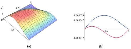
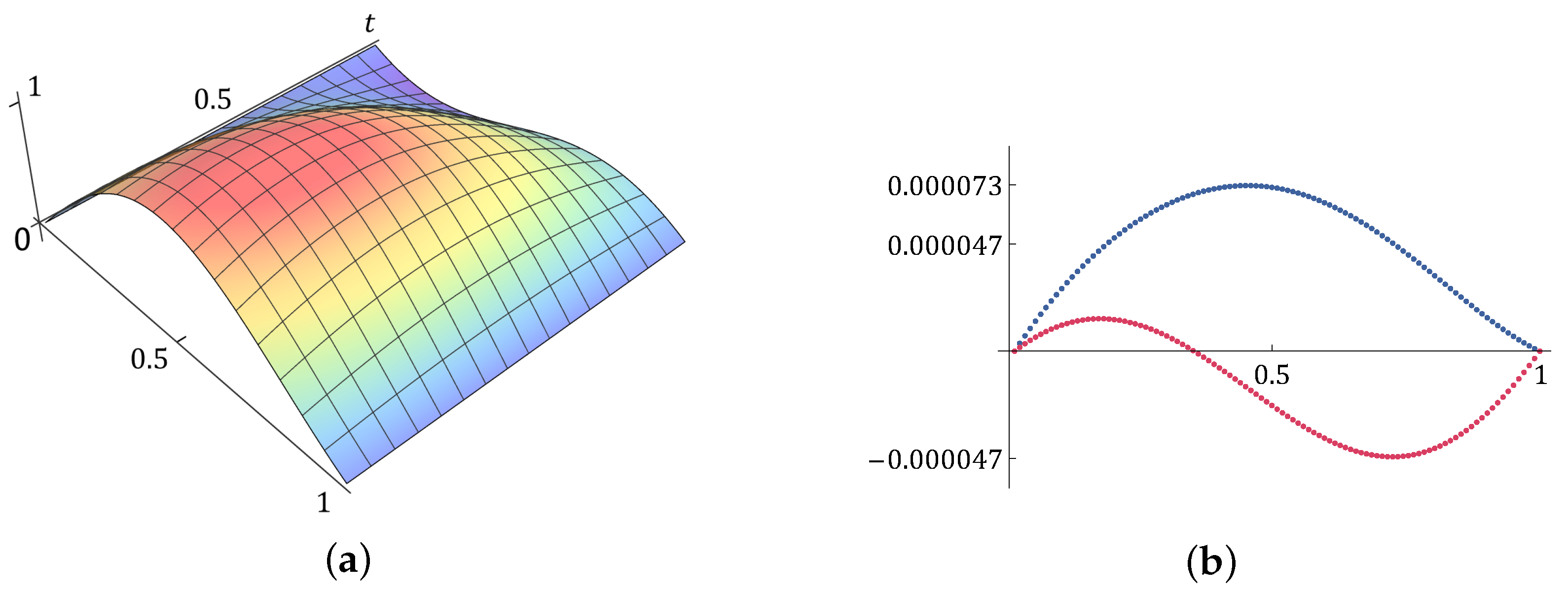
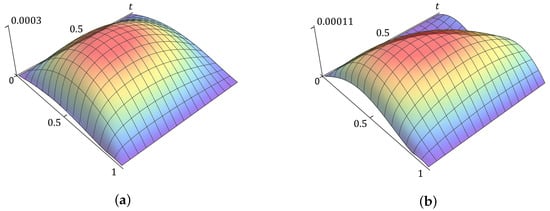
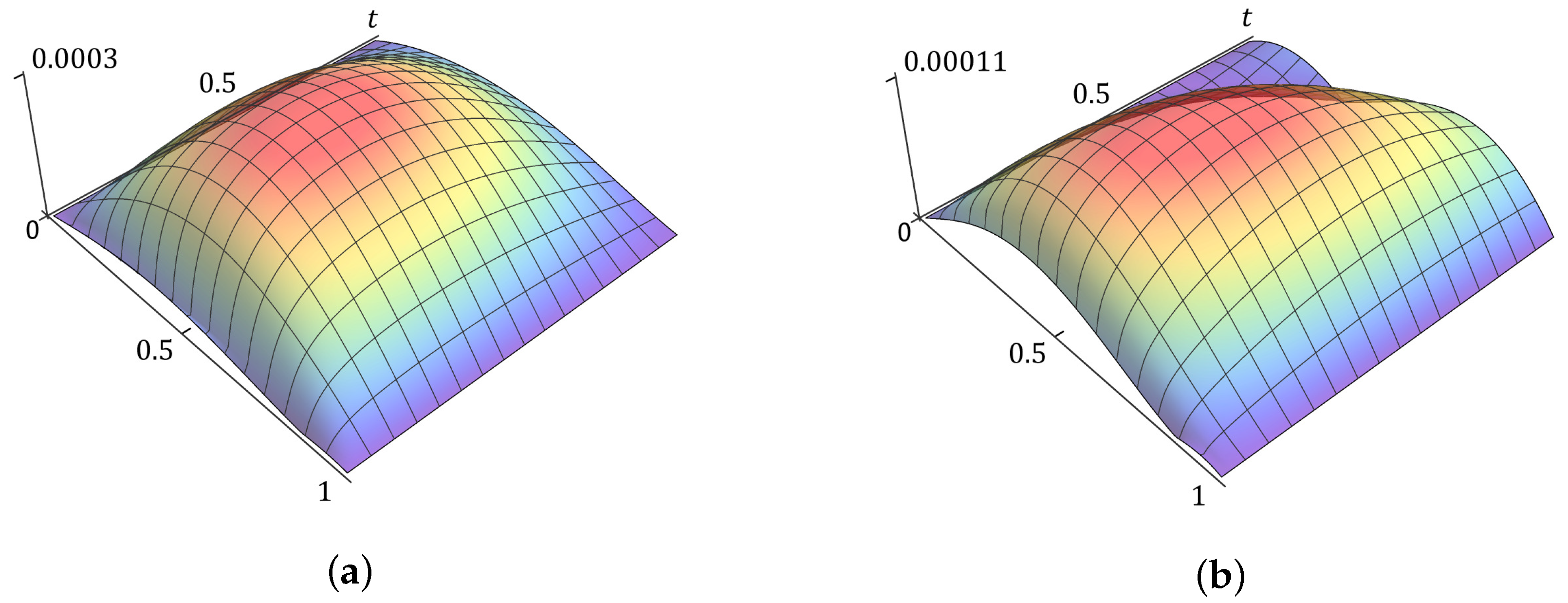
Figure 1a shows the discrete solution of the TFSE in Example 1, computed using the corrected L1 scheme (32) with $\alpha =0.75$, $d=1$, and $h=\tau =0.01$. The errors of classical L1 scheme and the corrected L1 scheme at the final time level $(n=N)$ are compared on Figure 1b. The first rows of Table 1 and Table 2 report the errors corresponding to the parameter values specified above. The error distributions corresponding to the L1 scheme and the corrected L1 scheme are shown in Figure 2. The performance of the classical L1 scheme and the corrected L1 scheme (32) is compared in Table 1 and Table 2 using four error measures: the global maximum error, the error at the first time level, the error at the final time level, and the maximum-in-time discrete spatial $l_2$-error. The comparison is performed under the simultaneous mesh refinement $h=\tau$. For the corrected L1 scheme, the numerical solution at the first time level $n=1$ is computed using (28), whereas for the classical L1 scheme, it is computed using the standard L1 approximation of the fractional derivative.

$$f_1^{\left(\alpha \right)}={\displaystyle \frac{{\tau }^{-\alpha }}{2^{1-\alpha }\Gamma (2-\alpha )}}\left(f_1-f_0\right)+\mathcal{O}\left({\tau }^{2-\alpha }\right).$$

Figure 1. Numerical solution obtained with the corrected L1 scheme (32) for the TFSE in Example 1 with $\alpha =0.75$, $d=1$, and $h=\tau =0.01$ (a), and the error distributions at the final time level for the L1 scheme (blue) and the corrected L1 scheme (red) (b).

Table 1. Numerical results for L1 scheme (32) for the TFSE in Example 1 with $\alpha =0.75$.

h = $\mathit{\tau }$	Global Error	Order	First-Row Error	Order	Last-Row Error	Order	Max Spatial ${\mathit{l}}_2$ Error	Order
$0.01$	$2.9819\times {10}^{-4}$	$0.8440$	$5.8108\times {10}^{-5}$	$1.3875$	$7.2793\times {10}^{-5}$	$1.2814$	$2.1218\times {10}^{-4}$	$0.8574$
$0.005$	$1.4384\times {10}^{-4}$	$1.0518$	$1.8500\times {10}^{-5}$	$1.6511$	$3.3216\times {10}^{-5}$	$1.1319$	$1.0193\times {10}^{-4}$	$1.0576$
$0.0025$	$6.5104\times {10}^{-5}$	$1.1437$	$5.3438\times {10}^{-6}$	$1.7916$	$1.5043\times {10}^{-5}$	$1.1427$	$4.6046\times {10}^{-5}$	$1.1465$
$0.00125$	$2.8529\times {10}^{-5}$	$1.1903$	$1.4584\times {10}^{-6}$	$1.8734$	$6.6376\times {10}^{-6}$	$1.1804$	$2.0156\times {10}^{-5}$	$1.1918$
$0.000625$	$1.2284\times {10}^{-5}$	$1.2157$	$3.8461\times {10}^{-7}$	$1.9229$	$2.8738\times {10}^{-6}$	$1.2077$	$8.6739\times {10}^{-6}$	$1.2165$

Table 2. Numerical results for corrected L1 scheme (32) for the TFSE in Example 1 with $\alpha =0.75$.

h = $\mathit{\tau }$	Global Error	Order	First-Row Error	Order	Last-Row Error	Order	Max Spatial ${\mathit{l}}_2$ Error	Order
$0.01$	$1.0816\times {10}^{-4}$	$2.0294$	$3.1958\times {10}^{-5}$	$2.5614$	$4.6344\times {10}^{-5}$	$2.0294$	$7.4437\times {10}^{-5}$	$1.9961$
$0.005$	$2.7065\times {10}^{-5}$	$1.9987$	$5.2147\times {10}^{-6}$	$2.6155$	$1.1381\times {10}^{-5}$	$2.0256$	$1.8627\times {10}^{-5}$	$1.9986$
$0.0025$	$6.7674\times {10}^{-6}$	$1.9997$	$8.2587\times {10}^{-7}$	$2.6586$	$2.8024\times {10}^{-6}$	$2.0220$	$4.6583\times {10}^{-6}$	$1.9996$
$0.00125$	$1.6917\times {10}^{-6}$	$2.0001$	$1.2790\times {10}^{-7}$	$2.6909$	$6.9153\times {10}^{-7}$	$2.0188$	$1.1646\times {10}^{-6}$	$2.0000$
$0.000625$	$4.2283\times {10}^{-7}$	$2.0003$	$1.9503\times {10}^{-8}$	$2.7132$	$1.7096\times {10}^{-7}$	$2.0161$	$2.9110\times {10}^{-7}$	$2.0002$

Figure 2. Absolute error distributions obtained with the L1 scheme (a) and the corrected L1 scheme (b) for the TFSE in Example 1, with $\alpha =0.75$, $d=1$, and $h=\tau =0.01$.

At the first time level, the numerical error is $\mathcal{O}({\tau }^2+h^2)$ for the classical L1 scheme, whereas for the corrected L1 scheme it is $\mathcal{O}\left({\tau }^{\alpha }({\tau }^2+h^2)\right)$. The improvement in the accuracy of the numerical error relative to the underlying approximation error results from the factor ${\tau }^{\alpha }$ appearing in the discrete error equation. Consequently, under the simultaneous refinement $h=\tau$, the expected convergence orders are 2 and $2+\alpha$, respectively. The corresponding observed orders are computed from

$$\mathrm{Order}(h,\tau )={\log }_2{\displaystyle \frac{E(2h,2\tau )}{E(h,\tau )}}$$

where $E(h,\tau )$ denotes the error obtained with the spatial and temporal step sizes h and $\tau$, respectively.

The temporal and spatial convergence orders of the corrected L1 scheme (32) for $\alpha =0.2,0.5,$ and $0.8$ are given in Table 3 and Table 4, respectively. In the temporal convergence test, the spatial step is fixed at $h=0.0005$, whereas in the spatial convergence test, the time step is fixed at $\tau =0.001$. The observed orders, computed using the global discrete $l_2$-error, are given by

$${\mathrm{Order}}_{\tau }\left(\tau \right)={\log }_2{\displaystyle \frac{E\left(2\tau \right)}{E\left(\tau \right)}},{\mathrm{Order}}_h\left(h\right)={\log }_2{\displaystyle \frac{E\left(2h\right)}{E\left(h\right)}}.$$

Table 3. Global $l_2$ error and order in time of corrected L1 scheme (32) for the TFSE in Example 1.

h = 0.0005	α = 0.2		α = 0.5		α = 0.8		CPU (s)
$\tau$	Error	Order ($\tau$)	Error	Order ($\tau$)	Error	Order ($\tau$)
$1/8$	$6.82\times {10}^{-4}$	$2.5085$	$1.41\times {10}^{-3}$	$2.6281$	$1.89\times {10}^{-3}$	$2.7287$	$2.3168$
$1/16$	$1.26\times {10}^{-4}$	$2.4337$	$2.32\times {10}^{-4}$	$2.6064$	$2.93\times {10}^{-4}$	$2.6965$	$4.7262$
$1/32$	$2.53\times {10}^{-5}$	$2.3197$	$4.01\times {10}^{-5}$	$2.5360$	$4.82\times {10}^{-5}$	$2.6012$	$9.7639$
$1/64$	$5.56\times {10}^{-6}$	$2.1854$	$7.63\times {10}^{-6}$	$2.3926$	$8.83\times {10}^{-6}$	$2.4503$	$20.672$
$1/128$	$1.38\times {10}^{-6}$	$2.0086$	$1.70\times {10}^{-6}$	$2.1597$	$1.86\times {10}^{-6}$	$2.2459$	$48.065$

Table 4. Global $l_2$ error and order in space of corrected L1 scheme (32) for the TFSE in Example 1.

$\tau$ = 0.001	α = 0.2		α = 0.5		α = 0.8		CPU (s)
h	Error	Order (h)	Error	Order (h)	Error	Order (h)
$1/8$	$9.18\times {10}^{-3}$	$2.0496$	$9.36\times {10}^{-3}$	$2.0502$	$9.36\times {10}^{-3}$	$2.0502$	$53.524$
$1/16$	$2.27\times {10}^{-3}$	$2.0122$	$2.32\times {10}^{-3}$	$2.0124$	$2.32\times {10}^{-3}$	$2.0124$	$57.513$
$1/32$	$5.68\times {10}^{-4}$	$2.0030$	$5.79\times {10}^{-4}$	$2.0031$	$5.79\times {10}^{-4}$	$2.0030$	$64.205$
$1/64$	$1.41\times {10}^{-4}$	$2.0006$	$1.44\times {10}^{-4}$	$2.0006$	$1.44\times {10}^{-4}$	$2.0006$	$83.147$
$1/128$	$3.54\times {10}^{-5}$	$1.9996$	$3.61\times {10}^{-5}$	$1.9997$	$3.62\times {10}^{-5}$	$1.9997$	$133.92$

4. Conclusions

A second-order implicit difference scheme for the time-fractional subdiffusion equation has been constructed using a corrected L1 approximation (2) of the Caputo fractional derivative. The correction modifies only the first three convolution coefficients and therefore preserves the simple convolution structure of the classical L1 formula. The stability and convergence analysis is based on the properties of the generating function of the corrected coefficients and estimates for the associated discrete resolvent. The scheme is shown to be unconditionally stable, with no restriction coupling the temporal and spatial step sizes. Under the stated regularity assumptions, the implicit discrete solution is second-order convergent in both time and space. The results of the numerical experiments are consistent with the theoretical estimates. In particular, the classical L1 scheme exhibits the expected temporal order $2-\alpha$, whereas the corrected L1 scheme achieves second-order accuracy in the global maximum, final-time, and discrete spatial $l_2$ error measures. The numerical experiments illustrate the improvement in accuracy obtained through the correction of the initial convolution coefficients.

Possible extensions include equations with variable coefficients and nonhomogeneous boundary conditions, multidimensional problems, and solutions with limited regularity near the initial time. Fast algorithms for evaluating the convolution history may also be considered to reduce the computational cost for long-time simulations.

References

- Metzler, R.; Klafter, J. The random walk’s guide to anomalous diffusion: A fractional dynamics approach. Phys. Rep. 2000, 339, 1–77. [Google Scholar] [CrossRef] [Scilit]
- Sierociuk, D.; Dzieliński, A.; Sarwas, G.; Petráš, I.; Podlubny, I.; Škovránek, T. Modelling heat transfer in heterogeneous media using fractional calculus. Philos. Trans. R. Soc. A Math. Phys. Eng. Sci. 2013, 371, 20120146. [Google Scholar] [CrossRef] [Scilit] [PubMed]
- Bagley, R.L.; Torvik, P.J. A theoretical basis for the application of fractional calculus to viscoelasticity. J. Rheol. 1983, 27, 201–210. [Google Scholar] [CrossRef] [Scilit]
- Benson, D.A.; Wheatcraft, S.W.; Meerschaert, M.M. Application of a fractional advection-dispersion equation. Water Resour. Res. 2000, 36, 1403–1412. [Google Scholar] [CrossRef] [Scilit]
- Podlubny, I. Fractional-order systems and PIλDμ-controllers. IEEE Trans. Autom. Control 1999, 44, 208–214. [Google Scholar] [CrossRef] [Scilit]
- Ionescu, C.M.; Lopes, A.; Copot, D.; Machado, J.A.T.; Bates, J.H.T. The role of fractional calculus in modeling biological phenomena: A review. Commun. Nonlinear Sci. Numer. Simul. 2017, 51, 141–159. [Google Scholar] [CrossRef] [Scilit]
- Scalas, E.; Gorenflo, R.; Mainardi, F. Fractional calculus and continuous-time finance. Phys. A Stat. Mech. Appl. 2000, 284, 376–384. [Google Scholar] [CrossRef] [Scilit]
- Oldham, K.B.; Spanier, J. The Fractional Calculus: Theory and Applications of Differentiation and Integration to Arbitrary Order; Academic Press: New York, NY, USA, 1974; p. 140. [Google Scholar]
- Lin, Y.; Xu, C. Finite difference/spectral approximations for the time-fractional diffusion equation. J. Comput. Phys. 2007, 225, 1533–1552. [Google Scholar] [CrossRef] [Scilit]
- Jin, B.; Lazarov, R.; Zhou, Z. An analysis of the L1 scheme for the subdiffusion equation with nonsmooth data. IMA J. Numer. Anal. 2016, 36, 197–221. [Google Scholar] [CrossRef] [Scilit]
- Stynes, M. A survey of the L1 scheme in the discretisation of time-fractional problems. Numer. Math. Theory Methods Appl. 2022, 15, 1173–1192. [Google Scholar] [CrossRef] [Scilit]
- Dimitrov, Y.; Georgiev, S.; Miryanov, R.; Todorov, V. Convergence of the L1 two-term equation scheme. J. Phys. Conf. Ser. 2023, 2675, 012027. [Google Scholar] [CrossRef] [Scilit]
- Xiao, J.; Chen, Y.; Li, Z.; Zeng, F.; Zhang, Z. L1 Schemes for Time-Fractional Differential Equations: A Brief Survey and New Development. Numer. Math. Theory Methods Appl. 2025, 18, 544–574. [Google Scholar] [CrossRef] [Scilit]
- Lubich, C. Discretized fractional calculus. SIAM J. Math. Anal. 1986, 17, 704–719. [Google Scholar] [CrossRef] [Scilit]
- Cuesta, E.; Lubich, C.; Palencia, C. Convolution quadrature time discretization of fractional diffusion-wave equations. Math. Comput. 2006, 75, 673–696. [Google Scholar] [CrossRef] [Scilit]
- Gao, G.-H.; Sun, Z.-Z.; Zhang, H.-W. A new fractional numerical differentiation formula to approximate the Caputo fractional derivative and its applications. J. Comput. Phys. 2014, 259, 33–50. [Google Scholar] [CrossRef] [Scilit]
- Alikhanov, A.A. A new difference scheme for the time fractional diffusion equation. J. Comput. Phys. 2015, 280, 424–438. [Google Scholar] [CrossRef] [Scilit]
- Hu, C.-Y.; Lin, F.-R. A New L2 Type Difference Scheme for the Time-Fractional Diffusion Equation. Fractal Fract. 2025, 9, 325. [Google Scholar] [CrossRef] [Scilit]
- Ford, N.J.; Yan, Y. An approach to construct higher-order time discretisation schemes for time-fractional partial differential equations with nonsmooth data. Fract. Calc. Appl. Anal. 2017, 20, 1076–1105. [Google Scholar] [CrossRef] [Scilit]
- Jin, B.; Li, B.; Zhou, Z. Correction of high-order BDF convolution quadrature for fractional evolution equations. SIAM J. Sci. Comput. 2017, 39, A3129–A3152. [Google Scholar] [CrossRef] [Scilit]
- Liu, L.; Wang, J. Numerical methods for time-fractional subdiffusion equations: Convolution quadrature with block generalized Adams methods. Chaos 2025, 35, 093141. [Google Scholar] [CrossRef] [Scilit] [PubMed]
- Dimitrov, Y.; Georgiev, S.; Miryanov, R.; Todorov, V. Second-order L1 schemes for fractional differential equations. Fractal Fract. 2025, 9, 816. [Google Scholar] [CrossRef] [Scilit]
- Yang, Z.; Zeng, F. A corrected L1 method for a time-fractional subdiffusion equation. J. Sci. Comput. 2023, 95, 85. [Google Scholar] [CrossRef] [Scilit]
- Gracia, J.L.; O’Riordan, E.; Stynes, M. A fitted scheme for a Caputo initial-boundary value problem. J. Sci. Comput. 2018, 76, 583–609. [Google Scholar] [CrossRef] [Scilit]
- Shen, J.; Zeng, F.; Stynes, M. Second-order error analysis of the averaged L1 scheme for time-fractional initial-value and subdiffusion problems. Sci. China Math. 2024, 67, 1641–1664. [Google Scholar] [CrossRef] [Scilit]
- Chen, H.; Stynes, M. Error analysis of a second-order method on fitted meshes for a time-fractional diffusion problem. J. Sci. Comput. 2019, 79, 624–647. [Google Scholar] [CrossRef] [Scilit]
- Kopteva, N. Error analysis of the L1 method on graded and uniform meshes for a fractional-derivative problem in two and three dimensions. Math. Comput. 2019, 88, 2135–2155. [Google Scholar] [CrossRef] [Scilit]
- Milev, M.; Miryanov, R.; Dimitrov, Y. Efficient numerical methods for fractional- and integer-order ordinary differential equations. Axioms 2026, 15, 501. [Google Scholar] [CrossRef] [Scilit]
- Yan, Y.; Wang, Y.; Yan, Y.; Pani, A.K. Higher order time stepping methods for subdiffusion problems based on weighted and shifted Grünwald–Letnikov formulae with nonsmooth data. J. Sci. Comput. 2020, 83, 40. [Google Scholar] [CrossRef] [Scilit]
- Jiang, S.; Zhang, J.; Zhang, Q.; Zhang, Z. Fast evaluation of the Caputo fractional derivative and its applications to fractional diffusion equations. Commun. Comput. Phys. 2017, 21, 650–678. [Google Scholar] [CrossRef] [Scilit]
- Liao, H.-L.; Yan, Y.; Zhang, J. Unconditional convergence of a fast two-level linearized algorithm for semilinear subdiffusion equations. J. Sci. Comput. 2019, 80, 1–25. [Google Scholar] [CrossRef] [Scilit]
- Sun, T.; Li, T.-Y.; Sun, H.-W. All-at-once implementation for subdiffusion equation with time nonuniform mesh. J. Sci. Comput. 2026, 108, 71. [Google Scholar] [CrossRef] [Scilit]
- Patel, S.; Santra, S.; Behera, R. An efficient hybrid numerical approach for time-fractional sub-diffusion equations with multi-singularities. Numer. Algorithms 2026, 102, 85–122. [Google Scholar] [CrossRef] [Scilit]
- Li, X.; Xu, C. A space-time spectral method for the time fractional diffusion equation. SIAM J. Numer. Anal. 2009, 47, 2108–2131. [Google Scholar] [CrossRef] [Scilit]
- Haslinger, F. Complex Analysis: A Functional Analytic Approach; De Gruyter: Berlin, Germany; Boston, MA, USA, 2017. [Google Scholar] [CrossRef] [Scilit]
- Folland, G.B. Real Analysis: Modern Techniques and Their Applications, 2nd ed.; Wiley: New York, NY, USA, 1999. [Google Scholar]
- Ponce, R. Time discretization of fractional subdiffusion equations via fractional resolvent operators. Comput. Math. Appl. 2020, 80, 69–92. [Google Scholar] [CrossRef] [Scilit]
- Wilf, H.S. Generatingfunctionology, 3rd ed.; A K Peters: Wellesley, MA, USA, 2006. [Google Scholar]
- Tang, M. Generating functions and the solutions of full history recurrence equations. Electron. Notes Discret. Math. 2007, 29, 445–449. [Google Scholar] [CrossRef] [Scilit]
- Liao, H.-L.; Li, D.; Zhang, J. Sharp error estimate of the nonuniform L1 formula for linear reaction-subdiffusion equations. SIAM J. Numer. Anal. 2018, 56, 1112–1133. [Google Scholar] [CrossRef] [Scilit]
- Stynes, M.; O’Riordan, E.; Gracia, J.L. Error analysis of a finite difference method on graded meshes for a time-fractional diffusion equation. SIAM J. Numer. Anal. 2017, 55, 1057–1079. [Google Scholar] [CrossRef] [Scilit]
- Yuste, S.B. Weighted average finite difference methods for fractional diffusion equations. J. Comput. Phys. 2006, 216, 264–274. [Google Scholar] [CrossRef] [Scilit]
- Varah, J.M. A lower bound for the smallest singular value of a matrix. Linear Algebra Appl. 1975, 11, 3–5. [Google Scholar] [CrossRef] [Scilit]
- Kolotilina, L.Y. Bounds for the infinity norm of the inverse for certain M- and H-matrices. Linear Algebra Appl. 2009, 430, 692–702. [Google Scholar] [CrossRef] [Scilit]
- Rudin, W. Real and Complex Analysis, 3rd ed.; McGraw-Hill: New York, NY, USA, 1987. [Google Scholar]
Disclaimer/Publisher’s Note: The statements, opinions and data contained in all publications are solely those of the individual author(s) and contributor(s) and not of MDPI and/or the editor(s). MDPI and/or the editor(s) disclaim responsibility for any injury to people or property resulting from any ideas, methods, instructions or products referred to in the content. |
© 2026 by the authors. Licensee MDPI, Basel, Switzerland. This article is an open access article distributed under the terms and conditions of the Creative Commons Attribution (CC BY) license.