Dynamic Analysis of a 2-out-of-6:G Repairable System with Preventive Maintenance

Abstract

This paper develops a 2-out-of-6:G repairable system with state-dependent preventive maintenance (PM) for functioning components. The 2-out-of-6:G configuration is adopted as a representative nontrivial case of the general k-out-of-n:G system, since it retains the essential features of component redundancy, multiple failure states, and a critical pre-failure state while remaining analytically tractable. When only two components remain functioning, PM is activated with probability $\beta$ to reduce the risk of an immediate system breakdown caused by an additional failure. Using the supplementary variable method, the model is formulated as an abstract Cauchy problem. Within the $C_0$-semigroup framework, the main operator is proved to generate a positive contraction $C_0$-semigroup, ensuring the existence and uniqueness of a positive solution. By combining Greiner’s boundary perturbation method with spectral analysis, the strong convergence of the solution to the steady-state solution is established. Numerical simulations further illustrate the theoretical results and demonstrate the influence of preventive maintenance on system reliability performance.

1. Introduction

Reliability theory draws on multiple disciplines and focuses on the analysis and evaluation of the ability of engineering systems to perform their required functions under specified operating conditions and within a given period of time. Through mathematical modeling and quantitative analysis, it provides an important theoretical basis for evaluating system reliability, identifying potential failure risks, and improving operational stability. With the increasing complexity of modern engineering systems, reliability analysis has become an essential tool not only for system design and performance assessment but also for developing effective maintenance strategies.

Traditional reliability models are often developed under simplified assumptions, such as independent component failures, prescribed failure and repair mechanisms, and corrective maintenance initiated only after component failure. In many such models, the system ceases operation once the number of failed components exceeds a specified threshold, while no maintenance action is taken on functioning components before system breakdown. These limitations have motivated the development of more flexible maintenance policies and modeling approaches. Barlow [1] established classical preventive maintenance models based on renewal reward theory and introduced age-based replacement and periodic maintenance policies, laying an important foundation for subsequent maintenance optimization studies. In a related methodological development, Gaver [2] treated repair time as a supplementary variable, thereby extending the analysis of repairable reliability systems to generally distributed repair times beyond the restrictive exponential assumption. Toshio [3] introduced imperfect preventive maintenance, while Goel et al. [4] developed a two-unit parallel repairable system incorporating minor repair, major repair, and stochastic preventive maintenance, and derived several reliability measures using the Laplace transform method. These developments gradually shifted reliability modeling from purely corrective and idealized maintenance mechanisms toward more realistic preventive and state-dependent maintenance frameworks.

With the progressive development of preventive maintenance theory [5,6], substantial research has been conducted on preventive maintenance strategies for k-out-of-n:G repairable systems, cold standby systems, and other repairable systems under different failure and maintenance mechanisms [7,8,9,10,11]. In particular, threshold- and state-based preventive maintenance policies have been introduced to trigger maintenance according to the number of failed components or specific system states [12,13,14]. Hybrid online and offline preventive maintenance strategies, as well as preventive maintenance for cold standby systems with partial failures, have also been extensively investigated [15,16,17,18]. Zhang et al. [19] developed a dual-layer nested preventive maintenance strategy and modeled the system using a multi-phase Markov process, while Wang et al. [20] established a three-state component model incorporating component degradation, periodic perfect maintenance, and corrective maintenance for a k-out-of-n:G system. Recent studies have further considered more flexible condition- and state-dependent maintenance policies for k-out-of-n systems. Liu et al. [21] developed a condition-based maintenance policy with non-periodic inspections for k-out-of-n:G systems. Li et al. [22] investigated a repairable k-out-of-n:G retrial system with two failure modes and preventive maintenance. Qi et al. [23] studied preventive maintenance optimization for weighted k-out-of-n:G systems, while Ning et al. [24] considered the joint optimization of preventive maintenance and a state-dependent triggering mechanism for k-out-of-n:F systems with protective devices.

In practical maintenance operations, reaching a prescribed deterioration or failure threshold does not necessarily imply that preventive maintenance can always be performed immediately. The implementation of PM may depend on maintenance-resource availability, inspection decisions, operational scheduling, and other practical constraints. To represent such partial or uncertain activation of maintenance actions, a randomized state-dependent maintenance mechanism can be introduced. In the present model, whenever the system enters the critical operating state with exactly two functioning components, PM is selected with probability $\beta$, whereas corrective repair is selected with probability $1-\beta$. Therefore, $\beta \in [0,1]$ characterizes the propensity to activate PM at the critical state and should be interpreted as a maintenance-policy parameter rather than a physical failure or repair parameter.

Research on repairable systems subject to preventive maintenance has produced a substantial body of mathematical models and reliability measures. However, comparatively less attention has been devoted to the rigorous analysis of solutions for repairable systems combining generally distributed repair times with state-dependent preventive-maintenance decisions. In particular, for k-out-of-n:G systems involving a probabilistic maintenance decision at a critical operating state, the well-posedness and long-term convergence of the resulting supplementary-variable model have received relatively limited attention.

In 2001, Gupur [25] introduced $C_0$-semigroup methods into the analysis of a two-unit parallel reliability system described using the supplementary variable method [26] and established its well-posedness. Later studies by Gupur and other researchers [27,28] extended this analytical framework to different reliability models, with particular attention to well-posedness and long-term dynamics. These studies established the existence of unique solutions and demonstrated their asymptotic stability. Haji et al. [29] subsequently obtained the asymptotic stability of the system solution through a boundary perturbation method. More recent investigations [30,31] addressed asymptotic stability from complementary operator-theoretic perspectives, including spectral analysis of the main operator along the imaginary axis and boundary perturbation arguments.

Motivated by these considerations, this paper develops a 2-out-of-6:G repairable system with a state-dependent probabilistic PM mechanism and investigates both its transient and asymptotic behavior. The main contributions of this study are summarized as follows.

(1) State-dependent preventive-maintenance mechanism. A critical-state maintenance mechanism is introduced. Whenever exactly two components remain functioning, preventive maintenance is activated with probability $\beta$, whereas corrective repair is selected with probability $1-\beta$. This formulation provides a probabilistic representation of partial or uncertain PM implementation at the critical operating state.

(2) Well-posedness of the Solution. Using the supplementary variable method, the reliability model is formulated as an abstract Cauchy problem on an appropriate Banach space. Within the $C_0$-semigroup framework, the main operator is shown to generate a positive contraction $C_0$-semigroup, thereby establishing the existence and uniqueness of a positive solution.

(3) Long-term convergence and numerical analysis. By combining Greiner’s boundary perturbation method with spectral analysis, the strong convergence of the solution to the steady-state solution is established. Numerical simulations are further performed to illustrate the theoretical results and to examine the influence of the PM activation probability $\beta$ on the reliability behavior of the system.

The remainder of this paper is organized as follows. Section 2 develops a mathematical model using the supplementary variable method under the prescribed assumptions and reformulates it as an abstract Cauchy problem on a Banach space. Section 3 investigates the well-posedness of the mathematical model by applying $C_0$-semigroup theory and Gupur’s mathematical approach [32]. Section 4 analyzes the asymptotic behavior of the model using Greiner’s boundary perturbation theory [33]. Section 5 presents a numerical example and the corresponding numerical simulations.

2. Mathematical Modeling of a 2-out-of-6:G Repairable System with Preventive Maintenance

This section presents the following assumptions and notations.

• The system consists of six identical components and one repairman.
• The system operates normally if at least 2 out of the 6 components function properly. The system fails when the number of failed components reaches five or more.
• One functioning component stops operating and cannot fail further during system downtime until the repair of failed components is completed. After repair, two functioning components resume operation simultaneously, and the system returns to the working state.
• Whenever exactly four components have failed and only two components remain functioning, preventive maintenance (PM) of the two functioning components is selected with probability $\beta$, whereas corrective repair of the failed components is selected with probability $1-\beta$, where $0\le \beta \le 1$.
• If the repairman selects preventive maintenance, the ongoing repair of the failed component is suspended. The repairman switches to maintaining the functioning components and resumes repairing the failed components after preventive maintenance is completed. All functioning components cease operation during preventive maintenance.
• Components receiving preventive maintenance are assumed not to experience failures within a short period after maintenance.
• Component lifetimes in the system follow an exponential distribution with parameter $\lambda$. The preventive maintenance time follows an exponential distribution with parameter $\theta$.
• The repair time Y of a failed component follows a general distribution

  $$G\left(t\right)=P\{Y\le t\},$$

  with density function

  $$g\left(t\right)={\displaystyle \frac{\mathrm{d}G\left(t\right)}{\mathrm{d}t}}=\varrho \left(t\right)\exp \left(-{\int }_0^t\varrho \left(\kappa \right)\mathrm{d}\kappa \right),$$

  where $\varrho \left(\kappa \right)$ denotes the repair rate of a failed component.

Remark 1.

The parameter β represents the state-dependent preventive-maintenance activation probability when the system enters the critical operating state with exactly four failed components and two functioning components. It is an exogenous maintenance-policy parameter rather than the success probability or effectiveness of preventive maintenance. In practice, β may reflect maintenance-resource availability, inspection decisions, maintenance scheduling, or other operational constraints that determine whether preventive maintenance can be implemented at the critical state. The limiting cases $\beta =0$ and $\beta =1$ correspond, respectively, to never and always selecting preventive maintenance upon entry into the critical state.

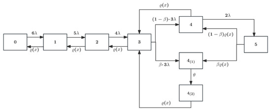
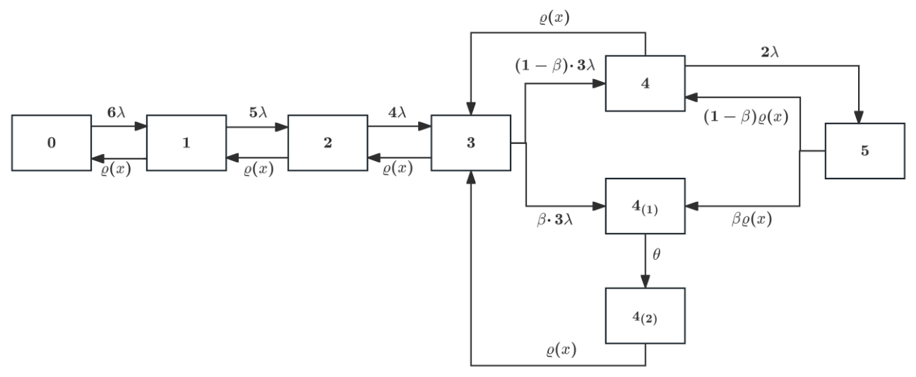
Based on the above assumptions and descriptions, the state transition diagram of the system is given in Figure 1.

Figure 1. State transition diagram of the system.

The random variables defined in the model are assumed to be mutually independent. A repaired component is regarded as being as good as new, and its post-repair lifetime follows the same distribution as that of a new component. Let the random variable $S\left(t\right)$ denote the system state at time t. The system states are defined based on the above assumptions as Repair time follows a general distribution. The stochastic process $\left\{S\right(t)\mid t\ge 0\}$ is not a one-dimensional Markov process. We introduce a supplementary variable $X\left(t\right)$. The variable $X\left(t\right)$ represents the elapsed repair time of the component under repair at time t. The augmented process $\left\{\right(S\left(t\right),X\left(t\right))\mid t\ge 0\}$ forms a two-dimensional continuous-time Markov process. We assume all components are intact at the initial time $t=0$. The variable $X\left(t\right)$ can thus be ignored under this initial condition. Let

$$\begin{array}{cc}\hfill p_0\left(t\right)& =P\left\{S\right(t)=0\}\hfill \\ \hfill & =P\left\{\mathrm{the}\mathrm{system}\mathrm{contains}0\mathrm{failed}\mathrm{components}\mathrm{at}\mathrm{time}\mathrm{t}\right\},\hfill \\ \hfill p_i(x,t)& =P\left\{S\right(t)=i,X(t)=x\}\hfill \\ \hfill & =P\{\mathrm{the}\mathrm{system}\mathrm{contains}i\mathrm{failed}\mathrm{components}\mathrm{and}\mathrm{the}\mathrm{elapsed}\mathrm{repair}\mathrm{time}\hfill \\ \hfill & \mathrm{of}\mathrm{the}\mathrm{unit}\mathrm{under}\mathrm{repair}\mathrm{equals}x\mathrm{at}\mathrm{time}t\},i=1,2,3,4,\hfill \\ \hfill p_{4_{\left(1\right)}}\left(t\right)& =P\{S\left(t\right)=4_{\left(1\right)}\}\hfill \\ \hfill & =P\{\mathrm{the}\mathrm{system}\mathrm{contains}4\mathrm{failed}\mathrm{components}\mathrm{and}\mathrm{preventive}\mathrm{maintenance}\hfill \\ \hfill & \mathrm{is}\mathrm{at}\mathrm{time}t\},\hfill \\ \hfill p_{4_{\left(2\right)}}(x,t)& =P\{S\left(t\right)=4_{\left(2\right)},X\left(t\right)=x\}\hfill \\ \hfill & =P\{\mathrm{after}\mathrm{the}\mathrm{completion}\mathrm{of}\mathrm{preventive}\mathrm{maintenance}\mathrm{the}\mathrm{system}\mathrm{contains}4\hfill \\ \hfill & \mathrm{failed}\mathrm{components}\mathrm{and}\mathrm{the}\mathrm{elapsed}\mathrm{repair}\mathrm{time}\mathrm{of}\mathrm{the}\mathrm{unit}\mathrm{under}\mathrm{equals}x\hfill \\ \hfill & \mathrm{at}\mathrm{time}t\},\hfill \\ \hfill p_5(x,t)& =P\left\{S\right(t)=5,X(t)=x\}\hfill \\ \hfill & =P\{\mathrm{the}\mathrm{system}\mathrm{contains}5\mathrm{failed}\mathrm{components}\mathrm{and}\mathrm{the}\mathrm{elapsed}\mathrm{repair}\mathrm{time}\hfill \\ \hfill & \mathrm{of}\mathrm{the}\mathrm{unit}\mathrm{under}\mathrm{repair}\mathrm{equals}x\mathrm{at}\mathrm{time}t\}.\hfill \end{array}$$

Based on the above analysis the mathematical model for the repairable 2-out-of-6:G system with preventive maintenance is established via the supplementary variable method and described by the following integro-partial differential equations.

$$\begin{array}{cc}\hfill & {\displaystyle \frac{\mathrm{d}{p}_0\left(t\right)}{\mathrm{d}t}}=-6\lambda p_0\left(t\right)+{\int }_0^{\infty }\varrho \left(x\right)p_1\left(x\right)\mathrm{d}x,\hfill \end{array}$$

(1)

$$\begin{array}{cc}\hfill & {\displaystyle \frac{\mathrm{d}{p}_1(x,t)}{\mathrm{d}t}}+{\displaystyle \frac{\mathrm{d}{p}_1(x,t)}{\mathrm{d}x}}=-[\varrho \left(x\right)+5\lambda )]p_1(x,t),\hfill \end{array}$$

(2)

$$\begin{array}{cc}\hfill & {\displaystyle \frac{\mathrm{d}{p}_i(x,t)}{\mathrm{d}t}}+{\displaystyle \frac{\mathrm{d}{p}_i(x,t)}{\mathrm{d}x}}=-[\varrho \left(x\right)+(6-i)\lambda )]p_i(x,t)+(7-i)\lambda p_{i-1}(x,t),i=2,3,\hfill \end{array}$$

(3)

$$\begin{array}{cc}\hfill & {\displaystyle \frac{\mathrm{d}{p}_4(x,t)}{\mathrm{d}t}}+{\displaystyle \frac{\mathrm{d}{p}_4(x,t)}{\mathrm{d}x}}=-[\varrho \left(x\right)+2\lambda )]p_4(x,t)+3(1-\beta )\lambda p_3(x,t),\hfill \end{array}$$

(4)

$$\begin{array}{cc}\hfill & {\displaystyle \frac{\mathrm{d}{p}_{4_{\left(1\right)}}\left(t\right)}{\mathrm{d}t}}=-\theta p_{4_{\left(1\right)}}\left(t\right)+3\beta \lambda {\int }_0^{\infty }{p}_3(x,t)\mathrm{d}x+\beta {\int }_0^{\infty }\varrho \left(x\right)p_5(x,t)\mathrm{d}x,\hfill \end{array}$$

(5)

$$\begin{array}{cc}\hfill & {\displaystyle \frac{\mathrm{d}{p}_{4_{\left(2\right)}}(x,t)}{\mathrm{d}t}}+{\displaystyle \frac{\mathrm{d}{p}_{4_{\left(2\right)}}(x,t)}{\mathrm{d}x}}=-\varrho \left(x\right)p_{4_{\left(2\right)}}(x,t),\hfill \end{array}$$

(6)

$$\begin{array}{cc}\hfill & {\displaystyle \frac{\mathrm{d}{p}_5(x,t)}{\mathrm{d}t}}+{\displaystyle \frac{\mathrm{d}{p}_5(x,t)}{\mathrm{d}x}}=-\varrho \left(x\right)p_5(x,t)+2\lambda p_4(x,t),\hfill \end{array}$$

(7)

The following expressions specify the initial and boundary conditions,

$$\begin{array}{cc}\hfill p_1(0,t)& =6\lambda p_0\left(t\right)+{\int }_0^{\infty }\varrho \left(x\right)p_2(x,t)\mathrm{d}x,\hfill \end{array}$$

(8)

$$\begin{array}{cc}\hfill p_2(0,t)& ={\int }_0^{\infty }\varrho \left(x\right)p_3(x,t)\mathrm{d}x,\hfill \end{array}$$

(9)

$$\begin{array}{cc}\hfill p_3(0,t)& ={\int }_0^{\infty }\varrho \left(x\right)p_4(x,t)\mathrm{d}x+{\int }_0^{\infty }\varrho \left(x\right)p_{4_{\left(2\right)}}(x,t)\mathrm{d}x,\hfill \end{array}$$

(10)

$$\begin{array}{cc}\hfill p_4(0,t)& =(1-\beta ){\int }_0^{\infty }\varrho \left(x\right)p_5(x,t)\mathrm{d}x,\hfill \end{array}$$

(11)

$$\begin{array}{cc}\hfill p_{4_{\left(2\right)}}(0,t)& =\theta p_{4_{\left(1\right)}}\left(t\right),\hfill \end{array}$$

(12)

$$\begin{array}{cc}\hfill p_5(0,t)& =0,\hfill \end{array}$$

(13)

where $(x,t)\in [0,\infty )\times [0,\infty )$.

Let

$$\Gamma =\left(\begin{array}{cccccccc}{e}^{-x}& 0& 0& 0& 0& 0& 0& 0\\ 6\lambda e^{-x}& \varrho \left(x\right)& 0& 0& 0& 0& 0& 0\\ 0& 0& \varrho \left(x\right)& 0& 0& 0& 0& 0\\ 0& 0& 0& 0& \varrho \left(x\right)& 0& \varrho \left(x\right)& 0\\ 0& 0& 0& 0& 0& 0& 0& (1-\beta )\varrho \left(x\right)\\ 0& 0& 0& 0& 0& e^{-x}& 0& 0\\ 0& 0& 0& 0& 0& \theta e^{-x}& 0& 0\\ 0& 0& 0& 0& 0& 0& 0& 0\end{array}\right),$$

Select the state space as

$$\mathcal{X}=\left\{p|\begin{array}{c}p=(p_0,p_{4_{\left(1\right)}},p_1,\dots ,p_4,p_{4_{\left(2\right)}},p_5)\in {\mathbb{R}}^2\times {\left[L^1[0,\infty )\right]}^6\hfill \\ \parallel p\parallel = |p_0| + |p_{{\left(4\right)}_{\left(1\right)}}|+{\displaystyle \sum _{i=1}^5}{\parallel p_i\parallel }_{L^1[0,\infty )}+{∥p_{{\left(4\right)}_{\left(2\right)}}∥}_{L^1[0,\infty )}\hfill \end{array}\right\}.$$

Obviously, $\mathcal{X}$ is a Banach space.

Define the operator $\mathcal{A}$ and its domain

$$\mathcal{A}p\left(x\right)=\left(\begin{array}{ccccc}-6\lambda & 0& 0& 0& 0\\ 0& A_1& 0& 0& 0\\ 0& 0& A_1& 0& 0\\ 0& 0& 0& -\theta & 0\\ 0& 0& 0& 0& A_1\end{array}\right),$$

where

$$A_1=\left(\begin{array}{cc}-\left[{\displaystyle \frac{\mathrm{d}}{\mathrm{d}x}}+\varrho \left(x\right)\right]& 0\\ 0& -\left[{\displaystyle \frac{\mathrm{d}}{\mathrm{d}x}}+\varrho \left(x\right)\right]\end{array}\right),$$

$$D\left(\mathcal{A}\right)=\left\{p\in \left(\mathcal{X}\right)|\begin{array}{c}{\displaystyle \frac{\mathrm{d}{p}_i(x,t)}{\mathrm{d}x}}\in L^1[0,\infty ),i=1,\dots ,5,4_{\left(2\right)},\hfill \\ p_i\left(x\right)\mathrm{is}\mathrm{an}\mathrm{absolutely}\mathrm{continuous}\mathrm{function},\hfill \\ \mathrm{and}\mathrm{satisfy}{p}_i\left(0\right)={\int }_0^{\infty }\Gamma p\left(x\right)dx\hfill \end{array}\right\},$$

$$\mathcal{H}p\left(x\right)=\left(\begin{array}{cccccccc}0& 0& 0& 0& 0& 0& 0& 0\\ 0& -5\lambda & 0& 0& 0& 0& 0& 0\\ 0& 5\lambda & -4\lambda & 0& 0& 0& 0& 0\\ 0& 0& 4\lambda & -3\lambda & 0& 0& 0& 0\\ 0& 0& 0& 3(1-\beta )\lambda & -2\lambda & 0& 0& 0\\ 0& 0& 0& 0& 0& 0& 0& 0\\ 0& 0& 0& 0& 0& 0& 0& 0\\ 0& 0& 0& 0& 2\lambda & 0& 0& 0\end{array}\right)\left(\begin{array}{c}{p}_0\\ p_1\left(x\right)\\ p_2\left(x\right)\\ p_3\left(x\right)\\ p_4\left(x\right)\\ p_{4_{\left(1\right)}}\\ p_{4_{\left(2\right)}}\left(x\right)\\ p_5\left(x\right)\end{array}\right),$$

$$D\left(\mathcal{H}\right)=\mathcal{X}.$$

Define the operator $\mathcal{B}$ and its domain

$$\mathcal{B}p\left(x\right)=\left(\begin{array}{c}{\int }_0^{\infty }\varrho \left(x\right)p_1\left(x\right)\mathrm{d}x\\ 0\\ 0\\ 0\\ 0\\ \beta (3\lambda {\int }_0^{\infty }{p}_3\mathrm{d}x+{\int }_0^{\infty }\varrho \left(x\right)p_5\mathrm{d}x)\\ 0\\ 0\end{array}\right),$$

$$D\left(\mathcal{B}\right)=\mathcal{X}.$$

Then the above-mentioned differential Equations (1)–(13) are reformulated as an abstract Cauchy problem in the Banach space $\mathcal{X}$.

$$\left\{\begin{array}{c}{\displaystyle \frac{\mathrm{d}p\left(t\right)}{\mathrm{d}t}}=(\mathcal{A}+\mathcal{H}+\mathcal{B})p\left(t\right),\forall t\in (0,\infty ),\hfill \\ p\left(0\right)=\left(1,0,0,0,0,0,0,0\right).\hfill \end{array}\right.$$

(14)

3. Well-Posedness of the System (14)

Theorem 1.

If $\overline{\mathcal{M}}=\underset{x\in [0,\infty )}{\sup }\varrho \left(x\right)<\infty$, then $\mathcal{A}+\mathcal{H}+\mathcal{B}$ generate a positive contraction $C_0$-semigroup $T\left(t\right)$.

Proof of Theorem 1.

Step 1: prove that when $\gamma >\overline{\mathcal{M}}$, ${(\gamma I-\overline{\mathcal{M}})}^{-1}$ exists and is bounded. For any $\tilde{y}\in \mathcal{X}$, Consider the equation $(\gamma I-\mathcal{A})p=\tilde{y}$, i.e.,

$$\begin{array}{cc}\hfill & (\gamma +6\lambda )p_0={\tilde{y}}_0,\hfill \end{array}$$

(15)

$$\begin{array}{cc}\hfill & (\gamma +{\displaystyle \frac{\mathrm{d}}{\mathrm{d}x}}+\varrho \left(x\right))p_i\left(x\right)={\tilde{y}}_i\left(x\right),i=1,\dots ,5,4_{\left(2\right)},\hfill \end{array}$$

(16)

$$\begin{array}{cc}\hfill & (\gamma +\theta )p_{4_{\left(1\right)}}={\tilde{y}}_{4_{\left(1\right)}},\hfill \end{array}$$

(17)

$$\begin{array}{cc}\hfill & p_1\left(0\right)=6\lambda p_0+{\int }_0^{\infty }\varrho \left(x\right)p_2\left(x\right)\mathrm{d}x,\hfill \end{array}$$

(18)

$$\begin{array}{cc}\hfill & p_2\left(0\right)={\int }_0^{\infty }\varrho \left(x\right)p_3\left(x\right)\mathrm{d}x,\hfill \end{array}$$

(19)

$$\begin{array}{cc}\hfill & p_3\left(0\right)={\int }_0^{\infty }\varrho \left(x\right)p_4\left(x\right)\mathrm{d}x+{\int }_0^{\infty }\varrho \left(x\right)p_{4_{\left(2\right)}}\left(x\right)\mathrm{d}x,\hfill \end{array}$$

(20)

$$\begin{array}{cc}\hfill & p_4\left(0\right)=(1-\beta ){\int }_0^{\infty }\varrho \left(x\right)p_5\left(x\right)\mathrm{d}x,\hfill \end{array}$$

(21)

$$\begin{array}{cc}\hfill & p_{4_{\left(2\right)}}\left(0\right)=-\theta p_{4_{\left(1\right)}},\hfill \end{array}$$

(22)

$$\begin{array}{cc}\hfill & p_5\left(0\right)=0.\hfill \end{array}$$

(23)

By solving Equations (15)–(17) we have

$$\begin{array}{cc}\hfill p_0& ={\displaystyle \frac{1}{\gamma +n\lambda }}{\tilde{y}}_0,\hfill \end{array}$$

(24)

$$\begin{array}{c}{p}_i\left(x\right)=a_i{e}^{-\gamma x-{\int }_0^x\varrho \left(\kappa \right)d\kappa }+e^{-\gamma x-{\int }_0^x\varrho \left(\kappa \right)\mathrm{d}\kappa }{\int }_0^x{\tilde{y}}_i\left(\zeta \right)e^{\gamma \zeta +{\int }_0^{\zeta }\varrho \left(\kappa \right)\mathrm{d}\kappa }\mathrm{d}\zeta ,\\ i=1,\dots ,5,4_{\left(2\right)},\hfill \end{array}$$

(25)

$$\begin{array}{cc}\hfill p_{4_{\left(1\right)}}& ={\displaystyle \frac{1}{\gamma +\theta }}{\tilde{y}}_{4_{\left(1\right)}}.\hfill \end{array}$$

(26)

Combining Equations (18)–(26) with Fubini theorem to estimate (with no loss of generality, assume $\gamma >0$)

$$\begin{array}{cc}\hfill \parallel p\parallel & = |p_0| + |p_{4_{\left(1\right)}}| +{\displaystyle \sum _{i=1}^5}\parallel p_i{\parallel }_{L^1[0,\infty ]}+ {\parallel p_{4_{\left(2\right)}}\parallel }_{L^1[0,\infty )}\hfill \\ \hfill & \le {\displaystyle \frac{|{\tilde{y}}_0|}{\gamma +6\lambda }}+{\displaystyle \frac{|{\tilde{y}}_{4_{\left(1\right)}}|}{\gamma +\theta }}+{\displaystyle \sum _{i=1}^5}\left[{\displaystyle \frac{\parallel {\tilde{y}}_i{\parallel }_{L^1[0,\infty )}}{\gamma }}+{\displaystyle \frac{\parallel {\tilde{y}}_{4_{\left(2\right)}}{\parallel }_{L^1[0,\infty )}}{\gamma }}\right]+\left[{\displaystyle \frac{|a_{4_{\left(2\right)}}|}{\gamma }}+{\displaystyle \frac{\parallel {\tilde{y}}_{4_{\left(2\right)}}{\parallel }_{L^1[0,\infty )}}{\gamma }}\right]\hfill \\ \hfill & \le {\displaystyle \frac{|{\tilde{y}}_0|}{\gamma +6\lambda }}+{\displaystyle \frac{|{\tilde{y}}_{4_{\left(1\right)}}|}{\gamma +\theta }}+{\displaystyle \sum _{i=1}^5}{\displaystyle \frac{\parallel {\tilde{y}}_i{\parallel }_{L^1[0,\infty )}}{\gamma }}+{\displaystyle \frac{\parallel {\tilde{y}}_{4_{\left(2\right)}}{\parallel }_{L^1[0,\infty )}}{\gamma }}\hfill \\ \hfill & +{\displaystyle \frac{6\lambda |{\tilde{y}}_0|}{\gamma (\gamma +6\lambda )}}+{\displaystyle \frac{\theta |{\tilde{y}}_{4_{\left(1\right)}}|}{\gamma (\gamma +\theta )}}\hfill \\ \hfill & +{\displaystyle \frac{\overline{\mathcal{M}}}{\gamma }}\left[{\displaystyle \sum _{i=2}^5}\parallel p_i{\parallel }_{L^1[0,\infty )}+ {\parallel p_{4_{\left(2\right)}}\parallel }_{L^1[0,\infty )}\right]\hfill \\ \hfill & \le {\displaystyle \frac{|{\tilde{y}}_0|}{\gamma +6\lambda }}+{\displaystyle \frac{|{\tilde{y}}_{4_{\left(1\right)}}|}{\gamma +\theta }}+{\displaystyle \sum _{i=1}^5}{\displaystyle \frac{\parallel {\tilde{y}}_i{\parallel }_{L^1[0,\infty )}}{\gamma }}+{\displaystyle \frac{\parallel {\tilde{y}}_{4_{\left(2\right)}}{\parallel }_{L^1[0,\infty )}}{\gamma }}\hfill \\ \hfill & +{\displaystyle \frac{6\lambda |{\tilde{y}}_0|}{\gamma (\gamma +6\lambda )}}+{\displaystyle \frac{\theta | {\tilde{y}}_{4_{\left(1\right)}}|}{\gamma (\gamma +\theta )}}\hfill \\ \hfill & +{\displaystyle \frac{\overline{\mathcal{M}}}{{\gamma }^2}}\left[{\displaystyle \sum _{i=2}^5}\parallel {\tilde{y}}_i{\parallel }_{L^1[0,\infty )}+{\parallel {\tilde{y}}_{4_{\left(2\right)}}\parallel }_{L^1[0,\infty )}\right]\hfill \\ \hfill & +{\displaystyle \frac{\overline{\mathcal{M}}\theta }{{\gamma }^2(\gamma +\theta )}}\left|{\tilde{y}}_{4_{\left(1\right)}}\right|\hfill \\ \hfill & +{\displaystyle \frac{{\overline{\mathcal{M}}}^2}{{\gamma }^2}}\left[{\displaystyle \sum _{i=3}^5}\parallel p_i{\parallel }_{L^1[0,\infty )}+ {\parallel p_{4_{\left(2\right)}}\parallel }_{L^1[0,\infty )}\right]\hfill \\ \hfill & \dots \hfill \\ \hfill & \le {\displaystyle \frac{|{\tilde{y}}_0|}{\gamma +6\lambda }}+{\displaystyle \frac{| {\tilde{y}}_{4_{\left(1\right)}}|}{\gamma +\theta }}+{\displaystyle \sum _{i=1}^5}{\displaystyle \frac{\parallel {\tilde{y}}_i{\parallel }_{L^1[0,\infty )}}{\gamma }}+{\displaystyle \frac{\parallel {\tilde{y}}_{4_{\left(2\right)}}{\parallel }_{L^1[0,\infty )}}{\gamma }}\hfill \\ \hfill & +{\displaystyle \frac{6\lambda |{\tilde{y}}_0|}{\gamma (\gamma +6\lambda )}}+{\displaystyle \frac{\theta | {\tilde{y}}_{4_{\left(1\right)}}|}{\gamma (\gamma +\theta )}}\hfill \\ \hfill & +{\displaystyle \frac{\overline{\mathcal{M}}}{{\gamma }^2}}\left[{\displaystyle \sum _{i=2}^5}\parallel {\tilde{y}}_i{\parallel }_{L^1[0,\infty )}+{\parallel {\tilde{y}}_{4_{\left(2\right)}}\parallel }_{L^1[0,\infty )}\right]\hfill \\ \hfill & +{\displaystyle \frac{\overline{\mathcal{M}}\theta }{{\gamma }^2(\gamma +\theta )}}|{\tilde{y}}_{4_{\left(1\right)}}|\hfill \\ \hfill & +{\displaystyle \frac{{\overline{\mathcal{M}}}^2}{{\gamma }^3}}\left[{\displaystyle \sum _{i=3}^5}\parallel {\tilde{y}}_i{\parallel }_{L^1[0,\infty )}+{\parallel {\tilde{y}}_{4_{\left(2\right)}}\parallel }_{L^1[0,\infty )}\right]\hfill \\ \hfill & +{\displaystyle \frac{{\overline{\mathcal{M}}}^2\theta }{{\gamma }^3(\gamma +\theta )}}\left|{\tilde{y}}_{4_{\left(1\right)}}\right|\hfill \\ \hfill & +{\displaystyle \frac{{\overline{\mathcal{M}}}^3}{{\gamma }^4}}\left[{\displaystyle \sum _{i=4}^5}\parallel {\tilde{y}}_i{\parallel }_{L^1[0,\infty )}+{\parallel {\tilde{y}}_{4_{\left(2\right)}}\parallel }_{L^1[0,\infty )}\right]\hfill \\ \hfill & +{\displaystyle \frac{{\overline{\mathcal{M}}}^3\theta }{{\gamma }^4(\gamma +\theta )}}\left|{\tilde{y}}_{4_{\left(1\right)}}\right|\hfill \\ \hfill & +{\displaystyle \frac{{\overline{\mathcal{M}}}^4}{{\gamma }^5}}\left[\parallel {\tilde{y}}_5{\parallel }_{L^1[0,\infty )}+{\parallel {\tilde{y}}_{4_{\left(2\right)}}\parallel }_{L^1[0,\infty )}\right]\hfill \\ \hfill & \le {\displaystyle \frac{1}{\gamma -\overline{\mathcal{M}}}}{\parallel \tilde{y}\parallel }_{L^1[0,\infty )}.\hfill \end{array}$$

(27)

Equation (27) shows that, when $\gamma >\overline{\mathcal{M}}$, ${\parallel (\gamma I-\mathcal{A})}^{-1}\parallel \le {\displaystyle \frac{1}{\gamma -\overline{\mathcal{M}}}}.$

Step 2: Prove that $D\left(\mathcal{A}\right)$ is dense in $\mathcal{X}$, let

$$Z=\left\{\begin{array}{cc}\hfill p\left(x\right)=& (p_0,p_1\left(x\right),\dots ,p_4\left(x\right),\hfill \\ & p_{4_{\left(1\right)}},p_{4_{\left(2\right)}}\left(x\right),p_5\left(x\right))\hfill \end{array}|\begin{array}{c}{p}_0\in \mathbb{R},p_{4_{\left(1\right)}}\in \mathbb{R},p_i\in C_0^1[0,\infty ),\hfill \\ \mathrm{there}\mathrm{exist}{c}_i>0\mathrm{such}\mathrm{that}\mathrm{for}\mathrm{all}\hfill \\ x\in [0,c_i],\mathrm{we}\mathrm{have}{p}_i\left(x\right)=0,\hfill \\ i=1,2,\dots ,5,4_{\left(2\right)}\hfill \end{array}\right\}.$$

It is known from Adams [34] that Z is dense in $\mathcal{X}$, i.e., $\overline{Z}=\mathcal{X}$. If one can prove that $Z\subset \overline{D\left(\mathcal{A}\right)}$, then

$$\begin{array}{cc}\hfill D\left(\mathcal{A}\right)\subset \mathcal{X}& \Rightarrow Z\subset \overline{D\left(\mathcal{A}\right)}\subset \mathcal{X}\Rightarrow \mathcal{X}=\overline{Z}\subset \overline{\overline{D\left(\mathcal{A}\right)}}\subset \overline{\mathcal{X}}=\mathcal{X}\hfill \\ & \Rightarrow \overline{D\left(\mathcal{A}\right)}=\overline{\overline{D\left(\mathcal{A}\right)}}=\mathcal{X}.\hfill \end{array}$$

Therefore, to prove the density of $D\left(\mathcal{A}\right)$ in $\mathcal{X}$, it suffices to show that $Z\subset \overline{D\left(\mathcal{A}\right)}$.

Let $p=(p_0,p_1,\cdots ,p_4,p_{4_{\left(1\right)}},p_{4_{\left(2\right)}},p_5)\in Z$, there exist positive constants $c_i>0$ such that $p_i\left(x\right)=0$ for all $\forall x\in [0,c_i]$. Accordingly, $p_i\left(x\right)=0$, for $x\in [0,s]$, where $0<s<\min \left\{c_i\right\},(i=1,\dots ,5,4_{\left(1\right)},4_{\left(2\right)})$. Define

$$\begin{array}{cc}\hfill f^s\left(0\right)& =\left(p_0,p_1^s\left(0\right),p_2^s\left(0\right),p_3^s\left(0\right),p_4^s\left(0\right),p_{4_{\left(1\right)}},p_{4_{\left(2\right)}}^s\left(0\right),p_5^s\left(0\right)\right),\hfill \\ & =(p_0,6\lambda p_0+{\int }_{2s}^{\infty }\varrho \left(x\right)p_2\left(x\right)\mathrm{d}x,{\int }_{2s}^{\infty }\varrho \left(x\right)p_3\left(x\right)\mathrm{d}x,{\int }_{2s}^{\infty }\varrho \left(x\right)p_4\left(x\right)\mathrm{d}x\hfill \\ & +{\int }_{2s}^{\infty }\varrho \left(x\right)p_{4_{\left(2\right)}}\left(x\right)\mathrm{d}x,(1-\beta ){\int }_{2s}^{\infty }\varrho \left(x\right)p_5\left(x\right)\mathrm{d}x,p_{4_{\left(1\right)}},\theta p_{4_{\left(1\right)}},0),\hfill \\ \hfill f^s\left(x\right)& =\left(p_0,f_1^s\left(x\right),\cdots f_4^s\left(x\right),p_{4_{\left(1\right)}},f_{4_{\left(2\right)}}^s\left(x\right),f_5^s\left(x\right)\right),\hfill \end{array}$$

$$\begin{array}{cc}\hfill f_i^s\left(x\right)& =\left\{\begin{array}{cc}{f}_i^s\left(0\right){\left(1-{\displaystyle \frac{x}{s}}\right)}^2,\hfill & x\in [0,s),\hfill \\ -{\displaystyle \frac{10}{s^4}}{f}_i^s\left(0\right){(x-s)}^2{(x-2s)}^2,\hfill & x\in [s,2s),\hfill \\ p_i\left(x\right),\hfill & x\in [2s,\infty ),\hfill \end{array}\right.i=1,\dots ,4,4_{\left(2\right)},\hfill \\ \hfill f_5^s\left(x\right)& =p_5\left(x\right),\forall x\in [0,\infty ).\hfill \end{array}$$

it is then easy to verify that $f^s\in D\left(\left(A\right)\right)$. Furthermore,

$$\begin{array}{cc}\hfill \parallel p-f^s\parallel & ={\displaystyle \sum _{i=1}^4}{\int }_0^{\infty }|p_i\left(x\right)-f_i^s\left(x\right)|\mathrm{d}x+{\int }_0^{\infty }|p_{4_{\left(2\right)}}\left(x\right)-f_{4_{\left(2\right)}}^s\left(x\right)|\mathrm{d}x\hfill \\ \hfill & =\left[{\displaystyle \sum _{i=1}^4}|f_i^s\left(0\right)|+|f_{4_{\left(2\right)}}^s\left(0\right)|\right]{\displaystyle \frac{2s}{3}}\to 0,s\to 0.\hfill \end{array}$$

This shows that $Z\subset \overline{D\left(\mathcal{A}\right)}$, $D\left(\mathcal{A}\right)$ is dense in $\mathcal{X}$. From the step 1, the step 2 and the Hille-Yosida theorem [32], $\mathcal{A}$ generates a $C_0$-semigroup.

Step 3: The bounded linearity of both $\mathcal{H}$ and $\mathcal{B}$ can be verified through elementary derivation. Therefore, it follows from the perturbation theorem [32] for $C_0$-semigroups that $\mathcal{A}+\mathcal{H}$ generates a $C_0$-semigroup $S\left(t\right)$, and $\mathcal{A}+\mathcal{H}+\mathcal{B}$ generates a $C_0$-semigroup $T\left(t\right)$.

Step 4: Prove that $\mathcal{A}+\mathcal{H}+\mathcal{B}$ is a dispersive operator. For $p\in D\left(\mathcal{A}\right)$, set

$$\varphi \left(x\right)=\left({\displaystyle \frac{{\left[p_0\right]}^{+}}{p_0}},{\displaystyle \frac{{\left[p_1\left(x\right)\right]}^{+}}{P_1\left(x\right)}},\cdots ,{\displaystyle \frac{{\left[p_{4_{\left(1\right)]}}\right]}^{+}}{p_{4_{\left(1\right)}}}},{\displaystyle \frac{{\left[p_{4_{\left(2\right)}}\left(x\right)\right]}^{+}}{p_{4_{\left(2\right)}}}},{\displaystyle \frac{{\left[p_5\left(x\right)\right]}^{+}}{p_5\left(x\right)}}\right),$$

where

$$\begin{array}{cc}\hfill {\left[p_0\right]}^{+}& =\left\{\begin{array}{cc}{p}_0,\hfill & p_0>0,\hfill \\ 0,\hfill & p_0\le 0,\hfill \end{array}\right.\hfill \\ \hfill \hfill {\left[p_{4_{\left(1\right)}}\right]}^{+}& =\left\{\begin{array}{cc}{p}_{4_{\left(1\right)}},\hfill & p_{4_{\left(1\right)}}>0,\hfill \\ 0,\hfill & p_{4_{\left(1\right)}}\le 0,\hfill \end{array}\right.\hfill \\ \hfill {\left[p_i\left(x\right)\right]}^{+}& =\left\{\begin{array}{cc}{p}_i\left(x\right),\hfill & p_i\left(x\right)>0,\hfill \\ 0,\hfill & p_i\left(x\right)\le 0,\hfill \end{array}\right.i=1,\dots ,5,4_{\left(2\right)},\hfill \end{array}$$

If we define

$$W_i=\left\{x\in [0,\infty )|p_i\left(x\right)>0\right\},Q_i=\left\{x\in [0,\infty )|p_i\left(x\right)\le 0\right\},i=1,\dots ,5,4_{\left(2\right)},$$

then

$$\begin{array}{cc}\hfill {\int }_0^{\infty }{\displaystyle \frac{\mathrm{d}{p}_i\left(x\right)}{\mathrm{d}x}}{\displaystyle \frac{{\left[p_i\left(x\right)\right]}^{+}}{p_i\left(x\right)}}\mathrm{d}x& ={\int }_{W_i}{\displaystyle \frac{\mathrm{d}{p}_i\left(x\right)}{\mathrm{d}x}}{\displaystyle \frac{{\left[p_i\left(x\right)\right]}^{+}}{p_i\left(x\right)}}\mathrm{d}x+{\int }_{Q_i}{\displaystyle \frac{\mathrm{d}{p}_i\left(x\right)}{\mathrm{d}x}}{\displaystyle \frac{{\left[p_i\left(x\right)\right]}^{+}}{p_i\left(x\right)}}\mathrm{d}x\hfill \\ \hfill & =-{\left[p_i\left(0\right)\right]}^{+},i=1,\dots ,5,4_{\left(2\right)}.\hfill \end{array}$$

(28)

For $p\in D\left(\mathcal{A}\right)$, using the above $\varphi$, Equations (18)–(23), Equation (28), and

$$\begin{array}{cc}\hfill {\int }_0^{\infty }\varrho \left(x\right)p_i\left(x\right)\mathrm{d}x& \le {\int }_0^{\infty }\varrho \left(x\right){\left[p_i\left(x\right)\right]}^{+}\mathrm{d}x,\hfill \\ \hfill {\int }_0^{\infty }{p}_i\left(x\right){\displaystyle \frac{{\left[p_{i+1}\left(x\right)\right]}^{+}}{p_{i+1}\left(x\right)}}\mathrm{d}x& \le {\int }_0^{\infty }{\left[p_i\left(x\right)\right]}^{+}\mathrm{d}x,i=1,\dots ,5,4_{\left(2\right)},\hfill \end{array}$$

we can estimate

$$\begin{array}{cc}\hfill ⟨(\mathcal{A}+\mathcal{H}+\mathcal{B})p,\varphi ⟩& =-6\lambda p_0+{\int }_0^{\infty }\varrho \left(x\right)p_1\left(x\right)\mathrm{d}x{\displaystyle \frac{{\left[p_0\right]}^{+}}{p_0}}\hfill \\ \hfill & +{\int }_0^{\infty }\left\{-{\displaystyle \frac{\mathrm{d}{p}_1\left(x\right)}{\mathrm{d}x}}-\left[\varrho \left(x\right)+5\lambda \right]p_1\left(x\right)\right\}{\displaystyle \frac{{\left[p_1\left(x\right)\right]}^{+}}{p_1\left(x\right)}}\mathrm{d}x\hfill \\ \hfill & +{\int }_0^{\infty }\left\{-{\displaystyle \frac{\mathrm{d}{p}_2\left(x\right)}{\mathrm{d}x}}-\left[\varrho \left(x\right)+4\lambda \right]p_2\left(x\right)+5\lambda p_1\left(x\right)\right\}{\displaystyle \frac{{\left[p_2\left(x\right)\right]}^{+}}{p_2\left(x\right)}}\mathrm{d}x\hfill \\ \hfill & +{\int }_0^{\infty }\left\{-{\displaystyle \frac{\mathrm{d}{p}_3\left(x\right)}{\mathrm{d}x}}-\left[\varrho \left(x\right)+3\lambda \right]p_3\left(x\right)+4\lambda p_2\left(x\right)\right\}{\displaystyle \frac{{\left[p_3\left(x\right)\right]}^{+}}{p_3\left(x\right)}}\mathrm{d}x\hfill \\ \hfill & +{\int }_0^{\infty }\left\{-{\displaystyle \frac{\mathrm{d}{p}_4\left(x\right)}{\mathrm{d}x}}-\left[\varrho \left(x\right)+2\lambda \right]p_4\left(x\right)+3\left(1-\beta \right)\lambda p_3\left(x\right)\right\}\hfill \\ \hfill & \times {\displaystyle \frac{{\left[p_4\left(x\right)\right]}^{+}}{p_4\left(x\right)}}\mathrm{d}x\hfill \\ \hfill & +\left\{-\theta p_{4_{\left(1\right)}}+3\beta \lambda {\int }_0^{\infty }{p}_3\left(x\right)\mathrm{d}x+\beta {\int }_0^{\infty }\varrho \left(x\right)p_5\left(x\right)\mathrm{d}x\right\}{\displaystyle \frac{{\left[p_{4_{\left(1\right)}}\right]}^{+}}{p_{4_{\left(1\right)}}}}\hfill \\ \hfill & +{\int }_0^{\infty }\left\{-{\displaystyle \frac{\mathrm{d}{p}_{4_{\left(2\right)}}\left(x\right)}{\mathrm{d}x}}-\varrho \left(x\right)p_{4_{\left(2\right)}}\left(x\right)\right\}{\displaystyle \frac{{\left[p_{4_{\left(2\right)}}\left(x\right)\right]}^{+}}{p_{4_{\left(2\right)}}\left(x\right)}}\mathrm{d}x\hfill \\ \hfill & +{\int }_0^{\infty }\left\{-{\displaystyle \frac{\mathrm{d}{p}_5\left(x\right)}{\mathrm{d}x}}-\varrho \left(x\right)p_5\left(x\right)+2\lambda p_4\left(x\right)\right\}{\displaystyle \frac{{\left[p_5\left(x\right)\right]}^{+}}{p_5\left(x\right)}}\mathrm{d}x\hfill \\ \hfill & \le \left({\displaystyle \frac{{\left[p_0\right]}^{+}}{p_0}}-1\right){\int }_0^{\infty }\varrho \left(x\right){\left[p_1\left(x\right)\right]}^{+}\mathrm{d}x\hfill \\ \hfill & \le 0.\hfill \end{array}$$

(29)

Equation (29) establishes the dispersivity of $\mathcal{A}+\mathcal{H}+\mathcal{B}$. Together with the results of Steps 1 and 2, Phillips’ theorem [32] implies that $\mathcal{A}+\mathcal{H}+\mathcal{B}$ generates a positive contraction $C_0$-semigroup. Since a $C_0$-semigroup is uniquely determined by its generator, the resulting semigroup coincides with $T\left(t\right)$. □

The dual space ${\mathcal{X}}^{*}$ of $\mathcal{X}$ is

$${\mathcal{X}}^{*}=\left\{q^{*}|\begin{array}{c}{q}^{*}=\left(q_0^{*},q_1^{*}\left(x\right),\dots q_4^{*}\left(x\right),q_{4_{\left(1\right)}}^{*},q_{4_{\left(2\right)}}^{*}\left(x\right),q_5^{*}\left(x\right)\right)\hfill \\ q^{*}\in \mathbb{R}\times L^{\infty }[0,\infty )\times \cdots \times L^{\infty }[0,\infty )\times \mathbb{R}\times L^{\infty }[0,\infty )\times L^{\infty }[0,\infty )\hfill \\ \parallel |q^{*}\parallel | =\sup \left\{\right|q_0^{*}|,\parallel q_1^{*}{\parallel }_{L^1[0,\infty )},\dots \parallel q_4^{*}{\parallel }_{L^1[0,\infty )},\left|q_{4_{\left(1\right)}}^{*}\right|,\hfill \\ \parallel q_{4_{\left(2\right)}}^{*}{\parallel }_{L^1[0,\infty )},{\parallel q_5^{*}\parallel }_{L^1[0,\infty )}\}\hfill \end{array}\right\}$$

Obviously ${\mathcal{X}}^{*}$ is a Banach space. Introduce a set in $\mathcal{X}$

$$Y=\left\{p\in \mathcal{X}{\displaystyle |}\begin{array}{c}p\left(x\right)=\left(p_0,p_1\left(x\right),\cdots ,p_4\left(x\right),p_{4_{\left(1\right)}},p_{4_{\left(2\right)}}\left(x\right),p_5\left(x\right)\right),\hfill \\ p_0\ge 0,p_{4_{\left(1\right)}}\ge 0,p_i\left(x\right)\ge 0,\hfill \\ i=1,\cdots ,5,4_{\left(2\right)}\forall x\in [0,\infty ).\hfill \end{array}\right\}$$

Then Y is a cone in $\mathcal{X}$. For $p\in D\left(\mathcal{A}\right)\cap Y$, define $q^{*}\left(x\right)=\parallel p\parallel (1,1,\dots ,1,1,1,1),$ then $q^{*}\in {\mathcal{X}}^{*}$, which yields

$$\begin{array}{cc}\hfill ⟨(\mathcal{A}+\mathcal{H}+\mathcal{B})p,q^{*}⟩& =\left\{-6\lambda p_0+{\int }_0^{\infty }\varrho \left(x\right)p_1\left(x\right)\mathrm{d}x\right\}\parallel p\parallel \hfill \\ \hfill & +{\int }_0^{\infty }\left\{-{\displaystyle \frac{\mathrm{d}{p}_1}{\mathrm{d}x}}-\left[\varrho \left(x\right)+5\lambda \right]p_1\left(x\right)\right\}\parallel p\parallel \mathrm{d}x+{\displaystyle \sum _{i=2}^3}{\int }_0^{\infty }\{-{\displaystyle \frac{\mathrm{d}{p}_i}{\mathrm{d}x}}\hfill \\ \hfill & -\left[\varrho \left(x\right)+(6-i)\lambda \right]p_i\left(x\right)+(7-i)\lambda p_{i-1}\left(x\right)\}\parallel p\parallel \mathrm{d}x\hfill \\ \hfill & +{\int }_0^{\infty }\left\{-{\displaystyle \frac{\mathrm{d}{p}_4}{\mathrm{d}x}}-\left[\varrho \left(x\right)+2\lambda \right]p_4\left(x\right)+3(1-\beta )\lambda p_3\left(x\right)\right\}\parallel p\parallel \mathrm{d}x\hfill \\ \hfill & +\left\{-\theta p_{4_{\left(1\right)}}+3\beta \lambda {\int }_0^{\infty }{p}_3\left(x\right)\mathrm{d}x+\beta {\int }_0^{\infty }\varrho \left(x\right)p_5\left(x\right)\mathrm{d}x\right\}\parallel p\parallel \hfill \\ \hfill & +{\int }_0^{\infty }\left\{-{\displaystyle \frac{\mathrm{d}{p}_{4_{\left(2\right)}}}{\mathrm{d}x}}-\varrho \left(x\right)p_{4_{\left(2\right)}}\left(x\right)\right\}\parallel p\parallel \mathrm{d}x\hfill \\ \hfill & +{\int }_0^{\infty }\left\{-{\displaystyle \frac{\mathrm{d}{p}_5}{\mathrm{d}x}}-\varrho \left(x\right)p_5\left(x\right)+2\lambda p_4\left(x\right)\right\}\parallel p\parallel \mathrm{d}x\hfill \\ \hfill & =0.\hfill \end{array}$$

This relation employs the property $p_i\in L^1[0,\infty )\Rightarrow p_i(\infty )=0,i=1,\dots ,5,4_{\left(2\right)}$.

The above result shows that $\mathcal{A}+\mathcal{H}+\mathcal{B}$ is a conservative operator with respect to the set

$$\Delta \left(p\right)=\{q^{*}\in X^{*}\mid ⟨p,q^{*}⟩={\parallel p\parallel }^2={\parallel q^{*}\parallel }^2\}.$$

Since $p\left(0\right)\in D\left({\mathcal{A}}^2\right)\cap Y$, the following conclusion follows from Fattorini’s theorem [35].

Theorem 2.

The operator $T\left(t\right)$ is an isometric operator for the initial value of system $(14)$. That is

$$\parallel T\left(t\right)p\left(0\right)\parallel = \parallel p\left(0\right)\parallel ,\forall t\in [0,\infty ).$$

Combining Theorem 1 and Theorem 2 yields the final conclusion of this section.

Theorem 3.

If $\overline{\mathcal{M}}=\underset{x\in [0,\infty )}{\sup }\mu \left(x\right)<\infty$, system $(14)$ admits a unique positive solution $p(x,t)$ such that

$$\parallel p(·,t)\parallel \le 1,\forall t\in [0,\infty ).$$

Proof. 

Since $p\left(0\right)\in D\left(\mathcal{A}\right)$, Theorem 1 together with Theorem 1.9 of [36] ensures that system (14) admits a unique positive solution $p(x,t)$. The solution is represented by

$$p(x,t)=T\left(t\right)p\left(0\right),\forall t\in [0,\infty ).$$

Combining this relation with Theorem 2 gives

$$\begin{array}{cc}\hfill \parallel p(·,t)\parallel & = \parallel T\left(t\right)p\left(0\right)\parallel \le \parallel p\left(0\right)\parallel =1,\forall t\in [0,\infty ).\hfill \end{array}$$

□

4. Asymptotic Behavior of Solutions of the System (14)

Define the maximal operator $\left({\mathcal{A}}_m,D\left({\mathcal{A}}_m\right)\right)$ and its domain as follows,

$${\mathcal{A}}_{m}p=\left(\begin{array}{cccccccc}-6\lambda & \psi & 0& 0& 0& 0& 0& 0\\ 0& -5\lambda +{\varphi }^2& 0& 0& 0& 0& 0& 0\\ 0& 5\lambda & -4\lambda +{\varphi }^2& 0& 0& 0& 0& 0\\ 0& 0& 4\lambda & -3\lambda +{\varphi }^2& 0& 0& 0& 0\\ 0& 0& 0& (1-\beta )3\lambda & -2\lambda +{\varphi }^2& 0& 0& 0\\ 0& 0& 0& 3\beta \lambda \pi & 0& -\theta & 0& \beta \psi \\ 0& 0& 0& 0& 0& 0& {\varphi }^2& 0\\ 0& 0& 0& 0& 0& 0& 2\lambda & {\varphi }^2\end{array}\right)\left(\begin{array}{c}{p}_0\\ p_1\left(x\right)\\ p_2\left(x\right)\\ p_3\left(x\right)\\ p_4\left(x\right)\\ p_{4_{\left(1\right)}}\left(x\right)\\ p_{4_{\left(2\right)}}\left(x\right)\\ p_5\left(x\right)\end{array}\right),$$

where

$$\begin{array}{cc}\hfill {\varphi }^{2}f& :=-{\displaystyle \frac{\mathrm{d}f\left(x\right)}{\mathrm{d}x}}-\varrho \left(x\right)f\left(x\right),\forall f\in W^{1,1}[0,\infty ),\hfill \\ \hfill {\varphi }_{i}f& :=-{\displaystyle \frac{\mathrm{d}f\left(x\right)}{\mathrm{d}x}}-\left[(6-i)\lambda +\varrho \left(x\right)\right]f\left(x\right),\forall f\in W^{1,1}[0,\infty ),\hfill \\ \hfill \psi f& :={\int }_0^{\infty }\varrho \left(x\right)f\left(x\right)\mathrm{d}x,\forall f\left(x\right)\in L^1[0,\infty ),\hfill \\ \hfill \pi f& :={\int }_0^{\infty }f\left(x\right)\mathrm{d}x,\forall f\left(x\right)\in L^1[0,\infty ),\hfill \end{array}$$

$$D\left({\mathcal{A}}_m\right)=\left\{p\in \mathcal{X}|\begin{array}{c}{\displaystyle \frac{\mathrm{d}{p}_i\left(x\right)}{\mathrm{d}x}}\in L^1[0,\infty ),p_i\left(x\right)\mathrm{is}\mathrm{an}\mathrm{absolutely}\mathrm{continuous}\mathrm{function},\hfill \\ {\displaystyle \sum _{i=1}^5}{∥{\displaystyle \frac{\mathrm{d}{p}_i}{\mathrm{d}x}}∥}_{L^1[0,\infty )}+{∥{\displaystyle \frac{\mathrm{d}{p}_{4_{\left(2\right)}}}{\mathrm{d}x}}∥}_{L^1[0,\infty )}<\infty \hfill \end{array}\right\}.$$

Select the boundary space of $\mathcal{X}$ as

$$\partial \mathcal{X}={\mathbb{R}}^6,$$

Define the boundary operators $\mathcal{K}$ and $\mathcal{G}$ as

$$\mathcal{K}:D\left({\mathcal{A}}_m\right)\to \partial \mathcal{X},$$

$$\mathcal{K}\left(\begin{array}{c}{p}_0\\ p_1\left(x\right)\\ p_2\left(x\right)\\ p_3\left(x\right)\\ p_4\left(x\right)\\ p_{4_{\left(1\right)}}\\ p_{4_{\left(2\right)}}\left(x\right)\\ p_5\left(x\right)\end{array}\right)=\left(\begin{array}{c}{p}_0\\ p_1\left(0\right)\\ p_2\left(0\right)\\ p_3\left(0\right)\\ p_4\left(0\right)\\ p_{4_{\left(1\right)}}\\ p_{4_{\left(2\right)}}\left(0\right)\\ p_5\left(x0\right)\end{array}\right),$$

and

$$\mathcal{G}:D\left({\mathcal{A}}_m\right)\to \partial \mathcal{X},$$

$$\mathcal{G}\left(\begin{array}{c}{p}_0\\ p_1\left(x\right)\\ p_2\left(x\right)\\ p_3\left(x\right)\\ p_4\left(x\right)\\ p_{4_{\left(1\right)}}\\ p_{4_{\left(2\right)}}\\ p_{n5}\left(x\right)\end{array}\right)=\left(\begin{array}{cccccccc}6\lambda & 0& \psi & 0& 0& 0& 0& 0\\ 0& 0& 0& \psi & 0& 0& 0& 0\\ 0& 0& 0& 0& \psi & 0& \psi & 0\\ 0& 0& 0& 0& 0& 0& 0& (1-\beta )\psi \\ 0& 0& 0& 0& 0& \theta & 0& 0\\ 0& 0& 0& 0& 0& 0& 0& 0\end{array}\right)\left(\begin{array}{c}{p}_0\\ p_1\left(x\right)\\ p_2\left(x\right)\\ p_3\left(x\right)\\ p_4\left(x\right)\\ p_{4_{\left(1\right)}}\\ p_{4_{\left(2\right)}}\left(x\right)\\ p_5\left(x\right)\end{array}\right),$$

where

$$\begin{array}{cc}\hfill \psi & :={\int }_0^{\infty }\varrho \left(x\right)f\left(x\right)\mathrm{d}x,\psi :L^1[0,\infty )\to \mathbb{R},\forall f\left(x\right)\in L^1[0,\infty ).\hfill \end{array}$$

If the operator is defined as

$$\begin{array}{cc}\hfill (\mathcal{A}+\mathcal{H}+\mathcal{B})p& ={\mathcal{A}}_{m}p,\hfill \\ \hfill \mathcal{D}\left(\mathcal{A}+\mathcal{H}+\mathcal{B}\right)& =\left\{p\in \mathcal{D}\left({\mathcal{A}}_m\right)|\mathcal{K}p=\mathcal{G}p\right\}.\hfill \end{array}$$

Then the system of differential Equations (1)–(13) can be rewritten as an abstract Cauchy problem like (14).

Define the operator $({\mathcal{A}}_0,D\left({\mathcal{A}}_0\right))$ by

$${\mathcal{A}}_{0}p={\mathcal{A}}_{m}p,D\left({\mathcal{A}}_0\right)=\left\{p\in D\left({\mathcal{A}}_m\right)\mid \mathcal{K}p=0\right\}.$$

For any $\tilde{y}\in \mathcal{X}$, consider the equation $(\gamma I-{\mathcal{A}}_0)p=\tilde{y}$. That is

$$\begin{array}{cc}\hfill (\gamma +6\lambda )p_0& ={\int }_0^{\infty }\varrho \left(x\right)p_1\left(x\right)\mathrm{d}x+{\tilde{y}}_0,\hfill \end{array}$$

(30)

$$\begin{array}{cc}\hfill {\displaystyle \frac{\mathrm{d}{p}_1\left(x\right)}{\mathrm{d}x}}& =-\left[\gamma +\varrho \left(x\right)+(n-1)\lambda \right]p_1\left(x\right)+{\tilde{y}}_1\left(x\right),\hfill \end{array}$$

(31)

$$\begin{array}{cc}\hfill {\displaystyle \frac{\mathrm{d}{p}_i\left(x\right)}{\mathrm{d}x}}& =-\left[\gamma +\varrho \left(x\right)+(6-i)\lambda \right]p_i\left(x\right)+(7-i)\lambda p_{i-1}\left(x\right)+{\tilde{y}}_i\left(x\right),i=2,3,\hfill \end{array}$$

(32)

$$\begin{array}{cc}\hfill {\displaystyle \frac{\mathrm{d}{p}_4\left(x\right)}{\mathrm{d}x}}& =-\left[\gamma +\varrho \left(x\right)+2\lambda \right]p_4\left(x\right)+3(1-\beta )\lambda p_3\left(x\right)+{\tilde{y}}_4\left(x\right),\hfill \end{array}$$

(33)

$$\begin{array}{cc}\hfill (\gamma +\theta )p_{4_{\left(1\right)}}& =3\beta \lambda {\int }_0^{\infty }{p}_3\left(x\right)\mathrm{d}x+\beta {\int }_0^{\infty }\varrho \left(x\right)p_5\left(x\right)\mathrm{d}x+{\tilde{y}}_{4_{\left(1\right)}},\hfill \end{array}$$

(34)

$$\begin{array}{cc}\hfill {\displaystyle \frac{d{p}_{4_{\left(2\right)}}\left(x\right)}{\mathrm{d}x}}& =-\left[\gamma +\varrho \left(x\right)\right]p_{4_{\left(2\right)}}\left(x\right)+{\tilde{y}}_{4_{\left(2\right)}}\left(x\right),\hfill \end{array}$$

(35)

$$\begin{array}{cc}\hfill {\displaystyle \frac{\mathrm{d}{p}_5\left(x\right)}{\mathrm{d}x}}& =-\left[\gamma +\varrho \left(x\right)\right]p_5\left(x\right)+2\lambda p_4\left(x\right)+{\tilde{y}}_5\left(x\right),\hfill \end{array}$$

(36)

$$\begin{array}{cc}\hfill p_i\left(0\right)& =1,\dots ,5,4_{\left(2\right)}.\hfill \end{array}$$

(37)

Solving (15)–(21) and employing (22) yields

$$\begin{array}{cc}\hfill p_0& ={\displaystyle \frac{1}{\gamma +6\lambda }}\left[{\int }_0^{\infty }\varrho \left(x\right)p_1\left(x\right)\mathrm{d}x+{\tilde{y}}_0\right],\hfill \end{array}$$

(38)

$$\begin{array}{cc}\hfill p_1\left(x\right)& =e^{-{\int }_0^x\left[\gamma +5\lambda +\varrho \left(\kappa \right)\right]\mathrm{d}\kappa }{\int }_0^x{\tilde{y}}_1\left(\kappa \right)e^{{\int }_0^{\kappa }\left[\gamma +5\lambda +\varrho \left(\zeta \right)\right]\mathrm{d}\zeta }\mathrm{d}\kappa ,\hfill \end{array}$$

(39)

$$\begin{array}{cc}\hfill p_i\left(x\right)& =e^{-{\int }_0^x\left[\gamma +(6-i)\lambda +\varrho \left(\kappa \right)\right]\mathrm{d}\kappa }[{\int }_0^x{\tilde{y}}_i\left(\kappa \right)e^{{\int }_0^{\kappa }\left[\gamma +(6-i)\lambda +\varrho \left(\zeta \right)\right]\mathrm{d}\zeta }\mathrm{d}\kappa \hfill \end{array}$$

(40)

$$\begin{array}{cc}\hfill & +{\int }_0^x(7-i)\lambda p_{i-1}\left(\kappa \right)e^{{\int }_0^{\kappa }\left[\gamma +(6-i)\lambda +\varrho \left(\zeta \right)\right]\mathrm{d}\zeta }\mathrm{d}\kappa ],i=2,3,\hfill \end{array}$$

(41)

$$\begin{array}{cc}\hfill p_4\left(x\right)& =e^{-{\int }_0^x\left[\gamma +2\lambda +\varrho \left(\kappa \right)\right]\mathrm{d}\kappa }[{\int }_0^x{\tilde{y}}_2\left(\kappa \right)e^{{\int }_0^{\kappa }\left[\gamma +2\lambda +\varrho \left(\zeta \right)\right]\mathrm{d}\zeta }\mathrm{d}\kappa \hfill \end{array}$$

(42)

$$\begin{array}{cc}\hfill & +{\int }_0^{x}3(1-\beta )\lambda p_3\left(\kappa \right)e^{{\int }_0^{\kappa }\left[\gamma +2\lambda +\varrho \left(\zeta \right)\right]\mathrm{d}\zeta }\mathrm{d}\kappa ],\hfill \end{array}$$

(43)

$$\begin{array}{cc}\hfill p_{{\left(4\right)}_{\left(1\right)}}& ={\displaystyle \frac{1}{\gamma +\theta }}\left[3\beta \lambda {\int }_0^{\infty }{p}_3\left(x\right)\mathrm{d}x+\beta {\int }_0^{\infty }\varrho \left(x\right)p_5\left(x\right)\mathrm{d}x+{\tilde{y}}_{{\left(4\right)}_{\left(1\right)}}\right],\hfill \end{array}$$

(44)

$$\begin{array}{cc}\hfill p_{{\left(4\right)}_{\left(2\right)}}& =e^{-{\int }_0^x\left[\gamma +\varrho \left(\kappa \right)\right]\mathrm{d}\kappa }{\int }_0^x{\tilde{y}}_{{\left(4\right)}_{\left(2\right)}}\left(\kappa \right)e^{{\int }_0^{\tau }\left[\gamma +\varrho \left(\zeta \right)\right]\mathrm{d}\zeta }\mathrm{d}\kappa ,\hfill \end{array}$$

(45)

$$\begin{array}{cc}\hfill p_5\left(x\right)& =e^{-{\int }_0^x\left[\gamma +\varrho \left(\kappa \right)\right]\mathrm{d}\kappa }\left[2\lambda {\int }_0^x{e}^{{\int }_0^{\kappa }\left[\gamma +\varrho \left(\zeta \right)\right]\mathrm{d}\kappa }{p}_4\left(\kappa \right)\mathrm{d}\kappa +{\int }_0^x{e}^{{\int }_0^{\kappa }\left[\gamma +\varrho \left(\zeta \right)\right]\mathrm{d}\zeta }{\tilde{y}}_5\left(\kappa \right)\mathrm{d}\kappa \right].\hfill \end{array}$$

(46)

For $\forall f\left(x\right)\in L^1[0,\infty )$, denote

$$\begin{array}{cc}\hfill E_i^{1}f\left(x\right)& =e^{-{\int }_0^x\left[\gamma +(6-i)\lambda +\varrho \left(\kappa \right)\right]\mathrm{d}\kappa }{\int }_0^{x}f\left(\kappa \right)e^{{\int }_0^{\kappa }\left[\gamma +(6-i)\lambda +\varrho \left(\zeta \right)\right]\mathrm{d}\zeta }\mathrm{d}\kappa ,i=1,2,\dots ,5,\hfill \\ \hfill E_{2}f\left(x\right)& =e^{-{\int }_0^x\left[\gamma +\varrho \left(\kappa \right)\right]\mathrm{d}\kappa }{\int }_0^{x}f\left(\kappa \right)e^{{\int }_0^{\kappa }\left[\gamma +\varrho \left(\zeta \right)\right]\mathrm{d}\zeta }\mathrm{d}\kappa .\hfill \end{array}$$

Combined with

$$\begin{array}{cc}\hfill \psi f\left(x\right)& ={\int }_0^{\infty }\varrho \left(x\right)f\left(x\right)\mathrm{d}x,\hfill \\ \hfill \pi f\left(x\right)& ={\int }_0^{\infty }f\left(x\right)\mathrm{d}x.\hfill \end{array}$$

Equations (23)–(28) are simplified as

$$\begin{array}{cc}\hfill & p_0={\displaystyle \frac{1}{\gamma +6\lambda }}\left[{\tilde{y}}_0+\psi E_1^1{\tilde{y}}_1\left(x\right)\right],\hfill \end{array}$$

(47)

$$\begin{array}{cc}\hfill & p_1\left(x\right)=E_1^1{\tilde{y}}_1\left(x\right),\hfill \end{array}$$

(48)

$$\begin{array}{cc}\hfill & p_i\left(x\right)=E_i^1{\tilde{y}}_i\left(x\right)+{\displaystyle \sum _{s=1}^{i-1}}{\displaystyle \prod _{l=s}^{i-1}}(6-l){\lambda }^{i-s}{\displaystyle \prod _{j=s}^i}{E}_j^1{\tilde{y}}_s\left(x\right)i=2,3,\hfill \end{array}$$

(49)

$$\begin{array}{cc}\hfill & p_4\left(x\right)=E_4^1{\tilde{y}}_4+(1-\beta ){\displaystyle \sum _{s=1}^3}{\displaystyle \prod _{l=s}^3}(6-l){\lambda }^{4-s}{\displaystyle \prod _{j=s}^4}{E}_j^1{\tilde{y}}_s\left(x\right),\hfill \end{array}$$

(50)

$$\begin{array}{c}{p}_{4_{\left(1\right)}}={\displaystyle \frac{1}{\gamma +\theta }}\{{\tilde{y}}_{4_{\left(1\right)}}+\beta \pi {\displaystyle \sum _{s=1}^3}{\displaystyle \prod _{l=s}^3}(6-l){\lambda }^{4-s}{\displaystyle \prod _{j=s}^3}{E}_j^1{\tilde{y}}_s\left(x\right)+\beta \psi E_2\hfill \\ \times \left[{\tilde{y}}_5\left(x\right)+2\lambda E_4^1{\tilde{y}}_4\left(x\right)+(1-\beta ){\displaystyle \sum _{s=1}^3}{\displaystyle \prod _{l=s}^4}(6-l){\lambda }^{5-s}{\displaystyle \prod _{j=s}^4}{E}_j^1{\tilde{y}}_s\left(x\right)\right]\},\hfill \end{array}$$

(51)

$$\begin{array}{cc}\hfill & p_{4_{\left(2\right)}}=E_2{\tilde{y}}_{4_{\left(2\right)}}\left(x\right),\hfill \end{array}$$

(52)

$$\begin{array}{cc}\hfill & p_5\left(x\right)=E_2{\tilde{y}}_5\left(x\right)+E_{2}2\lambda E_4^1{\tilde{y}}_4\left(x\right)+E_2(1-\beta ){\displaystyle \sum _{s=1}^3}{\displaystyle \prod _{l=s}^4}(6-l){\lambda }^{5-s}{\displaystyle \prod _{j=s}^4}{E}_j^1{\tilde{y}}_s\left(x\right).\hfill \end{array}$$

(53)

When $(\gamma I-{\mathcal{A}}_0)$ exists, (29)–(33) yield the expression for ${(\gamma I-{\mathcal{A}}_0)}^{-1}$

$${(\gamma I-{\mathcal{A}}_0)}^{-1}y=$$

$$\begin{array}{cc}\hfill & \left(\begin{array}{ccc}{\displaystyle \frac{1}{\gamma +6\lambda }}& {\displaystyle \frac{\psi E_1^1}{\gamma +6\lambda }}& 0\\ 0& E_1^1& 0\\ 0& 5\lambda {\displaystyle {\prod }_{l=1}^2}{E}_l^1& E_2^1\\ 0& 20{\lambda }^2{\displaystyle {\prod }_{l=1}^3}{E}_l^1& 4\lambda {\displaystyle {\prod }_{l=2}^3}{E}_l^1\\ 0& 60(1-\beta ){\lambda }^3{\displaystyle {\prod }_{l=1}^4}{E}_l^1& 12(1-\beta ){\lambda }^2{\displaystyle {\prod }_{l=2}^4}{E}_l^1\\ 0& {\displaystyle \frac{60\beta {\lambda }^3}{\gamma +\theta }}{\displaystyle {\prod }_{l=1}^3}{E}_l^1\left[\pi +2(1-\beta )\lambda \psi E_2{E}_4^1\right]& {\displaystyle \frac{12\beta {\lambda }^2}{\gamma +\theta }}{\displaystyle {\prod }_{l=2}^3}{E}_l^1\left[\pi +2(1-\beta )\lambda \psi E_2{E}_4^1\right]\\ 0& 0& 0\\ 0& 120(1-\beta ){\lambda }^4{E}_2{\displaystyle {\prod }_{l=1}^4}{E}_l^1& 24(1-\beta ){\lambda }^3{E}_2{\displaystyle {\prod }_{l=2}^4}{E}_l^1\end{array}\right.\hfill \\ \hfill & \left.\begin{array}{ccccc}0& 0& 0& 0& 0\\ 0& 0& 0& 0& 0\\ 0& 0& 0& 0& 0\\ E_3^1& 0& 0& 0& 0\\ 3(1-\beta )\lambda {\displaystyle {\prod }_{l=3}^4}{E}_l^1& E_4^1& 0& 0& 0\\ {\displaystyle \frac{3\beta \lambda }{\gamma +\theta }}{E}_3^1\left[\pi +2(1-\beta )\lambda \psi E_2{E}_4^1\right]& {\displaystyle \frac{2\beta \lambda \psi }{\gamma +\theta }}{E}_2{E}_4^1& {\displaystyle \frac{1}{\gamma +\theta }}& 0& {\displaystyle \frac{\beta \psi }{\gamma +\theta }}{E}_2\\ 0& 0& 0& E_2& 0\\ 6(1-\beta ){\lambda }^2{E}_2{\displaystyle {\prod }_{l=3}^4}{E}_l^1& 2\lambda E_2{E}_4^1& 0& 0& E_2\end{array}\right)\left(\begin{array}{c}{\tilde{y}}_0\\ {\tilde{y}}_1\left(x\right)\\ {\tilde{y}}_2\left(x\right)\\ {\tilde{y}}_3\left(x\right)\\ {\tilde{y}}_4\left(x\right)\\ {\tilde{y}}_{4_{\left(1\right)}}\\ {\tilde{y}}_{4_{\left(2\right)}}\left(x\right)\\ {\tilde{y}}_5\left(x\right)\end{array}\right).\hfill \end{array}$$

(54)

Lemma 1.

Let $\varrho \left(x\right):[0,\infty )\to [0,\infty )$ be a measurable function. Suppose that

$$0<\underset{x\in [0,\infty )}{\inf }\varrho \left(x\right)\le \varrho \left(x\right)\le \underset{x\in [0,\infty )}{\sup }\varrho \left(x\right)<\infty ,$$

then

$$\left\{\gamma \in \mathbb{C}|\mathrm{Re}\gamma +\underset{x\in [0,\infty )}{\inf }\varrho \left(x\right)>0\right\}\subset \rho \left({\mathcal{A}}_0\right).$$

Proof. 

For any

$$f\in L^1[0,\infty )\cap C_0^{\infty }[0,\infty ),$$

It is estimated that

$$\begin{array}{cc}\hfill {\int }_0^{\infty }\left|E_i^{1}f\left(x\right)\right|\mathrm{d}x& \le {\int }_0^{\infty }{e}^{-\left[\mathrm{Re}\gamma +(6-i)\lambda \right]x-{\int }_0^x\varrho \left(\kappa \right)\mathrm{d}\kappa }\times {\int }_0^x\left|f\left(\kappa \right)\right|e^{\left[\mathrm{Re}\gamma +(6-i)\lambda \right]\kappa +{\int }_0^{\kappa }\varrho \left(\zeta \right)\mathrm{d}\zeta }\mathrm{d}\kappa \mathrm{d}x\hfill \\ \hfill & ={\displaystyle \frac{-1}{\mathrm{Re}\gamma +(6-i)\lambda +\varrho \left(x\right)}}\times e^{-\left[\mathrm{Re}\gamma +(6-i)\lambda \right]x-{\int }_0^x{\varrho }_{(}\kappa )\mathrm{d}\kappa }\hfill \\ \hfill & \times {\int }_0^x\left|f\left(\kappa \right)\right|e^{\left[\mathrm{Re}\gamma +(6-i)\lambda \right]\kappa +{\int }_0^{\kappa }\varrho \left(\zeta \right)\mathrm{d}\zeta }\mathrm{d}\kappa {|}_0^{\infty }+{\int }_0^{\infty }{\displaystyle \frac{1}{\mathrm{Re}\gamma +(6-i)\lambda +\varrho \left(x\right)}}\hfill \\ \hfill & \times e^{-\left[\mathrm{Re}\gamma +(6-i)\lambda \right]x-{\int }_0^x\varrho \left(\kappa \right)\mathrm{d}\kappa }\times e^{\left[\mathrm{Re}\gamma +(6-i)\lambda \right]x+{\int }_0^x\varrho \left(\kappa \right)\mathrm{d}\kappa }\left|f\left(x\right)\right|\mathrm{d}x\hfill \\ \hfill & \le {\displaystyle \frac{1}{\mathrm{Re}\gamma +(6-i)\lambda +\underset{x\in [0,\infty )}{\inf }\varrho \left(x\right)}}{\parallel f\parallel }_{L^1(0,\infty )}.\hfill \end{array}$$

This yields

$$\begin{array}{c}\hfill \parallel E_i^1\parallel \le {\displaystyle \frac{1}{\mathrm{Re}\gamma +(6-i)\lambda +\underset{x\in [0,\infty )}{\inf }\varrho \left(x\right)}},i=1,\dots ,4,\end{array}$$

(55)

A similar argument gives

$$\begin{array}{c}\hfill \parallel E_2\parallel \le {\displaystyle \frac{1}{\mathrm{Re}\gamma +\underset{x\in [0,\infty )}{\inf }\varrho \left(x\right)}}.\end{array}$$

(56)

Adams [34] established the density of $C_0^{\infty }[0,\infty )$ in $L^1[0,\infty )$. Accordingly, Equations (55) and (56) remain valid for every $f\in L^1[0,\infty )$. For $\tilde{y}\in \mathcal{X}$, Equations (54)–(56) together with the condition $\mathrm{Re}\gamma +{\inf }_{x\in [0,\infty )}\varrho \left(x\right)>0$ yield the following estimate,

$$\begin{array}{cc}\hfill \parallel {(\gamma I-{\mathcal{A}}_0)}^{-1}\tilde{y}\parallel & \le {\displaystyle \frac{1}{|\gamma +6\lambda |}}\left|{\tilde{y}}_0\right|\hfill \\ \hfill & +[{\displaystyle \frac{1}{|\gamma +6\lambda |}}\parallel \psi \parallel \parallel E_1^1\parallel + \parallel E_1^1\parallel + 5\lambda {\displaystyle \prod _{l=1}^2}\parallel E_l^1\parallel \hfill \\ \hfill & + 20{\lambda }^2{\displaystyle \prod _{l=1}^3}\parallel E_l^1\parallel + 60(1-\beta ){\lambda }^3{\displaystyle \prod _{l=1}^4}\parallel E_l^1\parallel +{\displaystyle \frac{60\beta {\lambda }^3}{|\gamma +\theta |}}{\displaystyle \prod _{l=1}^3}\parallel E_l^1\parallel (\parallel \pi \parallel \hfill \\ \hfill & + 2(1-\beta )\lambda \parallel \psi \parallel \parallel E_2\parallel \parallel E_4^1\parallel + 120(1-\beta ){\lambda }^4\parallel E_2\parallel {\displaystyle \prod _{l=1}^4}\parallel E_l^1\parallel \left)\right]\hfill \\ \hfill & \times \parallel {\tilde{y}}_1{\parallel }_{L^1[0,\infty )}\hfill \\ \hfill & + [\parallel E_2^1\parallel + 4\lambda {\displaystyle \prod _{l=2}^3}\parallel E_l^1\parallel + 12(1-\beta ){\lambda }^2{\displaystyle \prod _{l=2}^4}\parallel E_l^1\parallel + {\displaystyle \frac{12\beta {\lambda }^2}{|\gamma +\theta |}}{\displaystyle \prod _{l=1}^3}\parallel E_l^1\parallel \hfill \\ \hfill & \times (\parallel \pi \parallel +2(1-\beta )\lambda \parallel \psi \parallel \parallel E_2\parallel \parallel E_4^1\parallel )+24(1-\beta ){\lambda }^3\parallel E_2\parallel {\displaystyle \prod _{l=2}^4}\parallel E_l^1\parallel ]\hfill \\ \hfill & \times \parallel {\tilde{y}}_2{\parallel }_{L^1[0,\infty )}\hfill \\ \hfill & + [\parallel E_3^1\parallel + 3(1-\beta )\lambda {\displaystyle \prod _{l=3}^4}\parallel E_l^1\parallel + {\displaystyle \frac{3\beta \lambda }{|\gamma +\theta |}}\parallel E_3^1\parallel (\parallel \pi \parallel +2(1-\beta )\lambda \hfill \\ \hfill & \times \parallel \psi \parallel \parallel E_2\parallel \parallel E_4^1\parallel )+6(1-\beta ){\lambda }^2\parallel E_2\parallel {\displaystyle \prod _{l=3}^4}\parallel E_l^1\parallel ]\parallel {\tilde{y}}_3{\parallel }_{L^1[0,\infty )}\hfill \\ \hfill & +\left[\parallel E_4^1\parallel +{\displaystyle \frac{2\beta \lambda }{|\gamma +\theta |}}\parallel \psi \parallel \parallel E_2\parallel \parallel E_4^1\parallel + 2\lambda \parallel E_2\parallel \parallel E_4^1\parallel \right]{\parallel {\tilde{y}}_4\parallel }_{L^1[0,\infty )}\hfill \\ \hfill & + {\displaystyle \frac{1}{|\gamma +\theta |}}\left|{\tilde{y}}_{4_{\left(1\right)}}\right|\hfill \\ \hfill & + \parallel E_2\parallel \parallel {\tilde{y}}_{4_{\left(2\right)}}{\parallel }_{L^1[0,\infty )}\hfill \\ \hfill & +\left[{\displaystyle \frac{\beta }{|\gamma +\theta |}}\parallel \psi \parallel \parallel E_1\parallel + \parallel E_2\parallel \right]{\parallel {\tilde{y}}_5\parallel }_{L^1[0,\infty )}\hfill \\ \hfill & \le {\displaystyle \frac{1}{|\gamma +6\lambda |}}\left|{\tilde{y}}_0\right|\hfill \\ \hfill & + [{\displaystyle \frac{1}{|\gamma +6\lambda |}}\parallel \psi \parallel \parallel E_1^1\parallel + \parallel E_1^1\parallel + 5\lambda {\displaystyle \prod _{l=1}^2}\parallel E_l^1\parallel +20{\lambda }^2{\displaystyle \prod _{l=1}^3}\parallel E_l^1\parallel \hfill \\ \hfill & + 60{\lambda }^3{\displaystyle \prod _{l=1}^4}\parallel E_l^1\parallel + {\displaystyle \frac{60\beta {\lambda }^3}{|\gamma +\theta |}}{\displaystyle \prod _{l=1}^3}\parallel E_l^1\parallel (\parallel \pi \parallel +2\lambda \parallel \psi \parallel \parallel E_2\parallel \parallel E_4^1\parallel \hfill \\ \hfill & + 120{\lambda }^4\parallel E_2\parallel {\displaystyle \prod _{l=1}^4}\parallel E_l^1\parallel \left)\right]\parallel {\tilde{y}}_1{\parallel }_{L^1[0,\infty )}\hfill \\ \hfill & +[\parallel E_2^1\parallel + 4\lambda {\displaystyle \prod _{l=2}^3}\parallel E_l^1\parallel + 12{\lambda }^2{\displaystyle \prod _{l=2}^4}\parallel E_l^1\parallel + {\displaystyle \frac{12\beta {\lambda }^2}{|\gamma +\theta |}}{\displaystyle \prod _{l=1}^3}\parallel E_l^1\parallel (\parallel \pi \parallel \hfill \\ \hfill & +2\lambda \parallel \psi \parallel \parallel E_2\parallel \parallel E_4^1\parallel )+24{\lambda }^3\parallel E_2\parallel {\displaystyle \prod _{l=2}^4}\parallel E_l^1\parallel ]\parallel {\tilde{y}}_2{\parallel }_{L^1[0,\infty )}\hfill \\ \hfill & +[\parallel E_3^1\parallel + 3\lambda {\displaystyle \prod _{l=3}^4}\parallel E_l^1\parallel + {\displaystyle \frac{3\beta \lambda }{|\gamma +\theta |}}\parallel E_3^1\parallel (\parallel \pi \parallel +2\lambda \parallel \psi \parallel \parallel E_2\parallel \parallel E_4^1\parallel )\hfill \\ \hfill & +6{\lambda }^2\parallel E_2\parallel {\displaystyle \prod _{l=3}^4}\parallel E_l^1\parallel ]\parallel {\tilde{y}}_3{\parallel }_{L^1[0,\infty )}\hfill \\ \hfill & +[\parallel E_4^1\parallel + {\displaystyle \frac{2\beta \lambda }{|\gamma +\theta |}}\parallel \psi \parallel \parallel E_2\parallel \parallel E_4^1\parallel + 2\lambda \parallel E_2\parallel \parallel E_4^1\parallel ]{\parallel {\tilde{y}}_4\parallel }_{L^1[0,\infty )}\hfill \\ \hfill & +{\displaystyle \frac{1}{|\gamma +\theta |}}\left|{\tilde{y}}_{4_{\left(1\right)}}\right|\hfill \\ \hfill & + \parallel E_2\parallel \parallel {\tilde{y}}_{4_{\left(2\right)}}{\parallel }_{L^1[0,\infty )}\hfill \\ \hfill & +\left[{\displaystyle \frac{\beta }{|\gamma +\theta |}}\parallel \psi \parallel \parallel E_1\parallel + \parallel E_2\parallel \right]{\parallel {\tilde{y}}_5\parallel }_{L^1[0,\infty )}\hfill \\ \hfill & \le {\displaystyle \frac{1}{|\gamma +6\lambda |}}\left|{\tilde{y}}_0\right|\hfill \\ \hfill & +{\displaystyle \sum _{i=1}^4}[{\displaystyle \frac{\underset{x\in [0,\infty )}{\sup }\mu \left(x\right)}{|\gamma +6\lambda |}}{\displaystyle \frac{1}{\mathrm{Re}\gamma +5\lambda +\underset{x\in [0,\infty )}{\inf }\mu \left(x\right)}}\hfill \\ \hfill & +{\displaystyle \sum _{m=0}^3}{\displaystyle \frac{1}{\mathrm{Re}\gamma +(5-m)\lambda +\underset{x\in [0,\infty )}{\inf }\mu \left(x\right)}}+{\displaystyle \frac{\beta }{|\gamma +\theta |}}\hfill \\ \hfill & +\left({\displaystyle \frac{\beta \underset{x\in [0,\infty )}{\sup }\mu \left(x\right)}{|\gamma +\theta |}}+1\right){\displaystyle \frac{1}{\mathrm{Re}\gamma +\underset{x\in [0,\infty )}{\inf }\mu \left(x\right)}}]{\parallel {\tilde{y}}_i\parallel }_{L^1[0,\infty )}\hfill \\ \hfill & +{\displaystyle \frac{1}{|\gamma +\theta |}}\left|{\tilde{y}}_{4\left(1\right)}\right|\hfill \\ \hfill & +{\displaystyle \frac{1}{\mathrm{Re}\gamma +\underset{x\in [0,\infty )}{\inf }\mu \left(x\right)}}{\parallel {\tilde{y}}_{4_{\left(2\right)}}\parallel }_{L^1[0,\infty )}\hfill \\ \hfill & +\left[\left({\displaystyle \frac{\beta \underset{x\in [0,\infty )}{\sup }\mu \left(x\right)}{|\gamma +\theta |}}+1\right){\displaystyle \frac{1}{\mathrm{Re}\gamma +\underset{x\in [0,\infty )}{\inf }\mu \left(x\right)}}\right]{\parallel {\tilde{y}}_5\parallel }_{L^1[0,\infty )}\hfill \\ \hfill & \le \sup \{{\displaystyle \frac{1}{|\gamma +\lambda |}},\hfill \\ \hfill & [{\displaystyle \frac{\underset{x\in [0,\infty )}{\sup }\mu \left(x\right)}{|\gamma +\lambda |}}{\displaystyle \frac{1}{\mathrm{Re}\gamma +5\lambda +\underset{x\in [0,\infty )}{\inf }\mu \left(x\right)}}\hfill \\ \hfill & +{\displaystyle \sum _{m=0}^3}{\displaystyle \frac{1}{\mathrm{Re}\gamma +(5-m)\lambda +\underset{x\in [0,\infty )}{\inf }\mu \left(x\right)}}\hfill \\ \hfill & +{\displaystyle \frac{\beta }{|\gamma +\theta |}}+\left({\displaystyle \frac{\beta \underset{x\in [0,\infty )}{\sup }\mu \left(x\right)}{|\gamma +\theta |}}+1\right){\displaystyle \frac{1}{\mathrm{Re}\gamma +\underset{x\in [0,\infty )}{\inf }\mu \left(x\right)}}],\hfill \\ \hfill & {\displaystyle \frac{1}{|\gamma +\theta |}}\}\parallel \tilde{y}\parallel \hfill \\ \hfill & <\infty .\hfill \end{array}$$

This relation establishes the conclusion of Lemma 1. □

Lemma 2.

Let $\varrho \left(x\right):[0,\infty )\to [0,\infty )$ are measurable and

$$0<\underset{x\in [0,\infty )}{\inf }\varrho \left(x\right)\le \varrho \left(x\right)\le \underset{x\in [0,\infty )}{\sup }\varrho \left(x\right)<\infty .$$

If

$$\gamma \in \left\{\gamma \in \mathbb{C}|\mathrm{Re}\gamma +\underset{x\in [0,\infty )}{\inf }\varrho \left(x\right)>0\right\},$$

then

$$\begin{array}{cc}\hfill & p\in \ker (\gamma I-{\mathcal{A}}_m)\hfill \\ \hfill & \iff \hfill \\ \hfill & p=\left(p_0,p_1,p_2,p_3,p_4,p_{4_{\left(1\right)}},p_{4_{\left(2\right)}},p_5\right),\hfill \\ \hfill p_0& ={\displaystyle \frac{1}{\gamma +6\lambda }}{\int }_0^{\infty }\varrho \left(x\right)a_1{e}^{-\left[\gamma +5\lambda \right]x-{\int }_0^x\varrho \left(\kappa \right)\mathrm{d}\kappa }\mathrm{d}x,\hfill \end{array}$$

(57)

$$\begin{array}{cc}\hfill p_1\left(x\right)& =a_1{e}^{-\left[\gamma +5\lambda \right]x-{\int }_0^x\varrho \left(\kappa \right)\mathrm{d}\kappa },\hfill \end{array}$$

(58)

$$\begin{array}{cc}\hfill p_i\left(x\right)& =e^{-\left[\gamma +(6-i)\lambda \right]x-{\int }_0^x\varrho \left(\kappa \right)\mathrm{d}\kappa }\hfill \\ & \times \left\{a_i+{\displaystyle \sum _{o=1}^{i-1}}{a}_{i-o}{\displaystyle \prod _{q=i-o}^{i-1}}(6-q)\left[{\displaystyle \sum _{r=1}^o}{\displaystyle \frac{{(-1)}^{r+1}\left(1-e^{-r\lambda x}\right)}{r!(o-r)!}}\right]\right\},2\le i\le 3,\end{array}$$

(59)

$$\begin{array}{cc}\hfill p_4\left(x\right)& =e^{-\left[\gamma +2\lambda \right]x-{\int }_0^x\varrho \left(\kappa \right)\mathrm{d}\kappa }\hfill \\ & \times \left\{a_4+(1-\beta ){\displaystyle \sum _{o=1}^3}{a}_{4-o}{\displaystyle \prod _{q=4-o}^3}(6-q)\left[{\displaystyle \sum _{r=1}^o}{\displaystyle \frac{{(-1)}^{r+1}\left(1-e^{-r\lambda x}\right)}{r!(o-r)!}}\right]\right\},\end{array}$$

(60)

$$\begin{array}{cc}\hfill p_{4_{\left(1\right)}}& ={\displaystyle \frac{3\beta \lambda }{\gamma +\theta }}{\int }_0^{\infty }{e}^{-\left[\gamma +3\lambda \right]x-{\int }_0^x\varrho \left(\kappa \right)\mathrm{d}\kappa }\hfill \\ \hfill & \times \left\{a_3+{\displaystyle \sum _{o=1}^2}{a}_{3-o}{\displaystyle \prod _{q=3-o}^2}(6-q)\left[{\displaystyle \sum _{r=1}^o}{\displaystyle \frac{{(-1)}^{r+1}\left(1-e^{-r\lambda x}\right)}{r!(o-r)!}}\right]\right\}\mathrm{d}x\hfill \\ \hfill & +{\displaystyle \frac{\beta }{\gamma +\theta }}{\int }_0^{\infty }\varrho \left(x\right)e^{-\gamma x-{\int }_0^x\varrho \left(\kappa \right)\mathrm{d}\kappa }\hfill \\ \hfill & \times \{a_5+a_4(1-e^{-2\lambda x})+2(1-\beta ){\displaystyle \sum _{o=1}^3}{a}_{4-o}{\displaystyle \prod _{q=4-o}^3}(6-q)\hfill \\ & \times {\displaystyle \sum _{r=1}^o}{\displaystyle \frac{{(-1)}^{r+1}}{r!(o-r)!}}\left({\displaystyle \frac{1-e^{-2\lambda }}{2}}-{\displaystyle \frac{1-e^{-(2+r)\lambda x}}{2+r}}\right)\}\mathrm{d}x,\hfill \end{array}$$

(61)

$$\begin{array}{cc}\hfill p_{4_{\left(2\right)}}\left(x\right)& =a_{4_{\left(2\right)}}{e}^{-{\int }_0^x\left[\gamma +\varrho \left(\kappa \right)\right]\mathrm{d}\kappa },\hfill \end{array}$$

(62)

$$\begin{array}{cc}\hfill p_5\left(x\right)& =e^{-{\int }_0^x\left[\gamma +\varrho \left(\kappa \right)\right]\mathrm{d}\kappa }\hfill \\ \hfill & \times \{a_5+a_4(1-e^{-2\lambda x})+2(1-\beta ){\displaystyle \sum _{o=1}^3}{a}_{4-o}{\displaystyle \prod _{q=4-o}^3}(6-q)\hfill \\ & \times \left[{\displaystyle \sum _{r=1}^o}{\displaystyle \frac{{(-1)}^{r+1}}{r!(o-r)!}}\left({\displaystyle \frac{1-e^{-2\lambda x}}{2}}-{\displaystyle \frac{1-e^{-(2+r)\lambda x}}{2+r}}\right)\right]\}.\hfill \end{array}$$

(63)

Proof. 

If $p\in (\gamma I-A_m)$, then $(\gamma I-A_m)p=0$, which is equivalent to

$$\begin{array}{cc}\hfill (\gamma +6\lambda )p_0& ={\int }_0^{\infty }\varrho \left(x\right)p_1\left(x\right)\mathrm{d}x,\hfill \end{array}$$

(64)

$$\begin{array}{cc}\hfill {\displaystyle \frac{\mathrm{d}{p}_1\left(x\right)}{\mathrm{d}x}}& =-\left[\gamma +\varrho \left(x\right)+5\lambda \right]p_1\left(x\right),\hfill \end{array}$$

(65)

$$\begin{array}{cc}\hfill {\displaystyle \frac{\mathrm{d}{p}_i\left(x\right)}{\mathrm{d}x}}& =-\left[\gamma +\varrho \left(x\right)+(6-i)\lambda \right]p_i\left(x\right)+(7-i)\lambda p_{i-1}\left(x\right)i=2,3,\hfill \end{array}$$

(66)

$$\begin{array}{cc}\hfill {\displaystyle \frac{\mathrm{d}{p}_4\left(x\right)}{\mathrm{d}x}}& =-\left[\gamma +\varrho \left(x\right)+2\lambda \right]p_4\left(x\right)+3(1-\beta )\lambda p_3\left(x\right),\hfill \end{array}$$

(67)

$$\begin{array}{cc}\hfill (\gamma +\theta )p_{4_{\left(1\right)}}& =3\beta \lambda {\int }_0^{\infty }{p}_3\left(x\right)\mathrm{d}x+\beta {\int }_0^{\infty }\varrho \left(x\right)p_5\left(x\right)\mathrm{d}x,\hfill \end{array}$$

(68)

$$\begin{array}{cc}\hfill {\displaystyle \frac{\mathrm{d}{p}_{4_{\left(2\right)}}\left(x\right)}{\mathrm{d}x}}& =-\left[\gamma +\varrho \left(x\right)\right]p_{4_{\left(2\right)}}\left(x\right),\hfill \end{array}$$

(69)

$$\begin{array}{cc}\hfill {\displaystyle \frac{\mathrm{d}{p}_5\left(x\right)}{\mathrm{d}x}}& =-\left[\gamma +\varrho \left(x\right)\right]p_5\left(x\right)+2\lambda p_4\left(x\right).\hfill \end{array}$$

(70)

By solving Equations (65)–(67) and Equations (69) and (70),

$$\begin{array}{cc}\hfill p_1\left(x\right)& =a_1{e}^{-\left[\gamma +5\lambda \right]x-{\int }_0^x\varrho \left(\kappa \right)\mathrm{d}\kappa },\hfill \end{array}$$

(71)

$$\begin{array}{cc}{p}_i\left(x\right)& =e^{-\left[\gamma +(6-i)\lambda \right]x-{\int }_0^x\varrho \left(\kappa \right)\mathrm{d}\kappa }\left[a_i+{\int }_0^x(7-i)\lambda p_{i-1}\left(\kappa \right)e^{\left[\gamma +(6-i)\lambda \right]\kappa +{\int }_0^{\kappa }\varrho \left(\zeta \right)\mathrm{d}\zeta }\mathrm{d}\kappa \right]\hfill \\ \hfill & i=2,3,\hfill \end{array}$$

(72)

$$\begin{array}{cc}\hfill p_4\left(x\right)& =e^{-\left[\gamma +2\lambda \right]x-{\int }_0^x\varrho \left(\kappa \right)\mathrm{d}\kappa }\left[a_4+{\int }_0^{x}3(1-\beta )\lambda p_3\left(\kappa \right)e^{\left[\gamma +2\lambda \right]\kappa +{\int }_0^{\kappa }\varrho \left(\zeta \right)\mathrm{d}\zeta }d\kappa \right],\hfill \end{array}$$

(73)

$$\begin{array}{cc}\hfill p_{4_{\left(2\right)}}\left(x\right)& =a_{4_{\left(2\right)}}{e}^{-\gamma x-{\int }_0^x\varrho \left(\kappa \right)\mathrm{d}\kappa },\hfill \end{array}$$

(74)

$$\begin{array}{cc}\hfill p_5\left(x\right)& =e^{-\gamma x-{\int }_0^x\varrho \left(\kappa \right)\mathrm{d}\kappa }\left[a_5+{\int }_0^{x}2\lambda p_4\left(\kappa \right)e^{\gamma \kappa +{\int }_0^{\kappa }\varrho \left(\zeta \right)\mathrm{d}\zeta }\mathrm{d}\kappa \right].\hfill \end{array}$$

(75)

Through repeated use of Equations (71)–(75),

$$\begin{array}{cc}\hfill p_1\left(x\right)& =a_1{e}^{-\left[\gamma +5\lambda \right]x-{\int }_0^x\varrho \left(\kappa \right)\mathrm{d}\kappa },\hfill \end{array}$$

(76)

$$\begin{array}{cc}\hfill p_i\left(x\right)& =e^{-\left[\gamma +(6-i)\lambda \right]x-{\int }_0^x\varrho \left(\kappa \right)\mathrm{d}\kappa }\hfill \\ \hfill & \times \left\{a_i+{\displaystyle \sum _{o=1}^{i-1}}{a}_{i-o}{\displaystyle \prod _{q=i-o}^{i-1}}(6-q)\left[{\displaystyle \sum _{r=1}^o}{\displaystyle \frac{{(-1)}^{r+1}\left(1-e^{-r\lambda x}\right)}{r!(o-r)!}}\right]\right\},2\le i\le 3,\hfill \end{array}$$

(77)

$$\begin{array}{cc}\hfill p_4\left(x\right)& =e^{-\left[\gamma +2\lambda \right]x-{\int }_0^x\varrho \left(\kappa \right)\mathrm{d}\kappa }\hfill \\ \hfill & \times \left\{a_4+(1-\beta ){\displaystyle \sum _{o=1}^3}{a}_{4-o}{\displaystyle \prod _{q=4-o}^3}(6-q)\left[{\displaystyle \sum _{r=1}^o}{\displaystyle \frac{{(-1)}^{r+1}\left(1-e^{-r\lambda x}\right)}{r!(o-r)!}}\right]\right\},\hfill \end{array}$$

(78)

$$\begin{array}{cc}\hfill p_{4_{\left(2\right)}}\left(x\right)& =a_{4_{\left(2\right)}}{e}^{-{\int }_0^x\left[\gamma +\varrho \left(\kappa \right)\right]\mathrm{d}\kappa },\hfill \end{array}$$

(79)

$$\begin{array}{cc}\hfill p_5\left(x\right)& =e^{-{\int }_0^x\left[\gamma +\varrho \left(\kappa \right)\right]\mathrm{d}\kappa }\hfill \\ \hfill & \times \{a_5+a_4(1-e^{-2\lambda x})+2(1-\beta ){\displaystyle \sum _{o=1}^3}{a}_{4-o}{\displaystyle \prod _{q=4-o}^3}(6-q)\hfill \\ \hfill & \times \left[{\displaystyle \sum _{r=1}^o}{\displaystyle \frac{{(-1)}^{r+1}}{r!(o-r)!}}\left({\displaystyle \frac{1-e^{-2\lambda x}}{2}}-{\displaystyle \frac{1-e^{-(2+r)\lambda x}}{2+r}}\right)\right]\}.\hfill \end{array}$$

(80)

Combining Equations (64), (68), (76), (77) and (80) yields

$$\begin{array}{cc}\hfill p_0& ={\displaystyle \frac{1}{\gamma +6\lambda }}{\int }_0^{\infty }\varrho \left(x\right)a_1{e}^{-\left[\gamma +5\lambda \right]x-{\int }_0^x\varrho \left(\kappa \right)\mathrm{d}\kappa }\mathrm{d}x,\hfill \end{array}$$

(81)

$$\begin{array}{cc}\hfill p_{4_{\left(1\right)}}& ={\displaystyle \frac{3\beta \lambda }{\gamma +\theta }}{\int }_0^{\infty }{e}^{-\left[\gamma +3\lambda \right]x-{\int }_0^x\varrho \left(\kappa \right)\mathrm{d}\kappa }\hfill \\ \hfill & \times \left\{a_3+{\displaystyle \sum _{o=1}^2}{a}_{3-o}{\displaystyle \prod _{q=3-o}^2}(6-q)\left[{\displaystyle \sum _{r=1}^o}{\displaystyle \frac{{(-1)}^{r+1}\left(1-e^{-r\lambda x}\right)}{r!(o-r)!}}\right]\right\}\mathrm{d}x\hfill \\ \hfill & +{\displaystyle \frac{\beta }{\gamma +\theta }}{\int }_0^{\infty }\varrho \left(x\right)e^{-\gamma x-{\int }_0^x\varrho \left(\kappa \right)\mathrm{d}\kappa }\hfill \\ \hfill & \times \{a_5+a_4(1-e^{-2\lambda x})+2(1-\beta ){\displaystyle \sum _{o=1}^3}{a}_{4-o}{\displaystyle \prod _{q=4-o}^3}(6-q)\hfill \\ \hfill & \times {\displaystyle \sum _{r=1}^o}{\displaystyle \frac{{(-1)}^{r+1}}{r!(o-r)!}}\left({\displaystyle \frac{1-e^{-2\lambda }}{2}}-{\displaystyle \frac{1-e^{-(2+r)\lambda x}}{2+r}}\right)\}\mathrm{d}x.\hfill \end{array}$$

(82)

Since $p\in \ker (\gamma I-{\mathcal{A}}_m)$ and $p\in D\left({\mathcal{A}}_m\right)$, the embedding theorem [34] gives

$$W^{1,1}[0,\infty )\hookrightarrow L^1[0,\infty ),$$

which yields

$$\begin{array}{cc}\hfill {\displaystyle \sum _{i=1}^5}|a_i|+|p_{4_{\left(2\right)}}|& ={\displaystyle \sum _{i=1}^5}|p_i\left(0\right)|+|p_{4_{\left(2\right)}}|\hfill \\ \hfill & \le {\displaystyle \sum _{i=1}^5}{\parallel p_i\parallel }_{L^{\infty }[0,\infty )}+{\parallel p_{4_{\left(2\right)}}\parallel }_{L^{\infty }[0,\infty )}\hfill \\ \hfill & \le {\displaystyle \sum _{i=1}^5}{\parallel p_i\parallel }_{L^1[0,\infty )}+{\displaystyle \sum _{i=1}^5}{∥{\displaystyle \frac{\mathrm{d}{p}_i}{\mathrm{d}x}}∥}_{L^1[0,\infty )}+{\parallel p_{4_{\left(2\right)}}\parallel }_{L^1[0,\infty )}+{∥{\displaystyle \frac{\mathrm{d}{p}_{4_{\left(2\right)}}}{\mathrm{d}x}}∥}_{L^1[0,\infty )}\hfill \\ \hfill & <\infty .\hfill \end{array}$$

(83)

The preceding relations verify Equations (57)–(63). Conversely, suppose that Equations (57)–(63) hold. Since

$$\mathrm{Re}\gamma +\underset{x\in [0,\infty )}{\inf }\varrho \left(x\right)>0,$$

the following bound is obtained,

$$\begin{array}{cc}\hfill \parallel p_1{\parallel }_{L^1[0,\infty )}& \le {\displaystyle \frac{1}{\mathrm{Re}\gamma +5\lambda +\underset{x\in [0,\infty )}{\inf }\varrho \left(x\right)}}\left|a_1\right|,\hfill \end{array}$$

(84)

$$\begin{array}{cc}\hfill \parallel p_i{\parallel }_{L^1[0,\infty )}& \le {\int }_0^{\infty }\left|a_i\right|e^{-\left[\mathrm{Re}\gamma +(6-i)\lambda \right]x-{\int }_0^x\varrho \left(\kappa \right)\mathrm{d}\kappa }\mathrm{d}x\hfill \\ \hfill & +{\displaystyle \sum _{o=1}^{i-1}}\left|a_{i-o}\right|{\displaystyle \prod _{q=i-o}^{i-1}}(6-q){\displaystyle \sum _{r=1}^o}{\displaystyle \frac{1}{r!(o-r)!}}\hfill \\ \hfill & \times {\int }_0^{\infty }\left(1-e^{-r\lambda x}\right)e^{-\left[\mathrm{Re}\gamma +(6-i)\lambda \right]x-{\int }_0^x\varrho \left(\kappa \right)\mathrm{d}\kappa }\mathrm{d}x\hfill \\ \hfill & \le {\displaystyle \frac{(i-1){\displaystyle \prod _{q=1}^{i-1}}(6-q)}{\mathrm{Re}\gamma +(6-i)\lambda +\underset{x\in [0,\infty )}{\inf }\varrho \left(x\right)}}{\displaystyle \sum _{o=0}^{i-1}}\left|a_{i-o}\right|,i=2,3,\hfill \end{array}$$

(85)

$$\begin{array}{cc}\hfill \parallel p_4{\parallel }_{L^1[0,\infty )}& \le {\int }_0^{\infty }\left|a_4\right|e^{-\left[\mathrm{Re}\gamma +2\lambda \right]x-{\int }_0^x\varrho \left(\kappa \right)\mathrm{d}\kappa }\mathrm{d}x\hfill \\ \hfill & +(1-\beta ){\displaystyle \sum _{o=1}^3}\left|a_{4-o}\right|{\displaystyle \prod _{q=4-o}^3}(6-q){\displaystyle \sum _{r=1}^o}{\displaystyle \frac{1}{r!(o-r)!}}\hfill \\ \hfill & \times {\int }_0^{\infty }\left(1-e^{-r\lambda x}\right)e^{-\left[\mathrm{Re}\gamma +2\lambda \right]x-{\int }_0^x\varrho \left(\kappa \right)\mathrm{d}\kappa }\mathrm{d}x\hfill \\ \hfill & \le {\displaystyle \frac{3{\displaystyle \prod _{q=1}^3}(6-q)}{\mathrm{Re}\gamma +2\lambda +\underset{x\in [0,\infty )}{\inf }\varrho \left(x\right)}}{\displaystyle \sum _{o=0}^3}\left|a_{4-o}\right|,\hfill \end{array}$$

(86)

$$\begin{array}{cc}\hfill \parallel p_{4_{\left(2\right)}}{\parallel }_{L^1[0,\infty )}& \le {\displaystyle \frac{1}{\mathrm{Re}\gamma +\underset{x\in [0,\infty )}{\inf }\varrho \left(x\right)}}|a_{4_{\left(2\right)}}|,\hfill \end{array}$$

(87)

$$\begin{array}{cc}\hfill \parallel p_5{\parallel }_{L^1[0,\infty )}& \le {\displaystyle \frac{1}{\mathrm{Re}\gamma +\underset{x\in [0,\infty )}{\inf }\varrho \left(x\right)}}| a_5| +{\displaystyle \frac{1}{\mathrm{Re}\gamma +\underset{x\in [0,\infty )}{\inf }\varrho \left(x\right)}}\left|a_4\right|\hfill \\ \hfill & +{\displaystyle \frac{3}{\mathrm{Re}\gamma +\underset{x\in [0,\infty )}{\inf }\varrho \left(x\right)}}{\displaystyle \sum _{o=1}^3}\left|a_{4-o}\right|{\displaystyle \prod _{q=1}^4}(6-q)\hfill \\ \hfill & \le {\displaystyle \frac{1}{\mathrm{Re}\gamma +\underset{x\in [0,\infty )}{\inf }\varrho \left(x\right)}}| a_5| +{\displaystyle \frac{3{\displaystyle \prod _{q=1}^4}(6-q)}{\mathrm{Re}\gamma +\underset{x\in [0,\infty )}{\inf }\varrho \left(x\right)}}{\displaystyle \sum _{o=0}^3}\left|a_{4-o}\right|,\hfill \end{array}$$

(88)

$$\begin{array}{cc}\hfill {\displaystyle \sum _{i=1}^5}\parallel p_i{\parallel }_{L^1[0,\infty )}+ {\parallel p_{4_{\left(2\right)}}\parallel }_{L^1[0,\infty )}& \le {\displaystyle \frac{1}{\mathrm{Re}\gamma +5\lambda +\underset{x\in [0,\infty )}{\inf }\varrho \left(x\right)}}\left|a_1\right|\hfill \\ \hfill & +{\displaystyle \sum _{i=2}^3}{\displaystyle \frac{(i-1){\displaystyle \prod _{q=1}^{i-1}}(6-q)}{\mathrm{Re}\gamma +(6-i)\lambda +\underset{x\in [0,\infty )}{\inf }\varrho \left(x\right)}}{\displaystyle \sum _{o=0}^{i-1}}\left|a_{i-o}\right|\hfill \\ \hfill & +{\displaystyle \frac{3{\displaystyle \prod _{q=1}^3}(6-q)}{\mathrm{Re}\gamma +2\lambda +\underset{x\in [0,\infty )}{\inf }\varrho \left(x\right)}}{\displaystyle \sum _{o=0}^3}\left|a_{4-o}\right|\hfill \\ \hfill & +{\displaystyle \frac{1}{\mathrm{Re}\gamma +\underset{x\in [0,\infty )}{\inf }\varrho \left(x\right)}}\left|a_{4_{\left(2\right)}}\right|\hfill \\ \hfill & +{\displaystyle \frac{1}{\mathrm{Re}\gamma +\underset{x\in [0,\infty )}{\inf }\varrho \left(x\right)}}| a_5| +{\displaystyle \frac{3{\displaystyle \prod _{q=1}^4}(6-q)}{\mathrm{Re}\gamma +\underset{x\in [0,\infty )}{\inf }\varrho \left(x\right)}}{\displaystyle \sum _{o=0}^3}\left|a_{4-o}\right|\hfill \\ \hfill & \le {\displaystyle \frac{1}{\mathrm{Re}\gamma +5\lambda +\underset{x\in [0,\infty )}{\inf }\varrho \left(x\right)}}\left|a_1\right|\hfill \\ \hfill & +{\displaystyle \frac{3^2{\displaystyle \prod _{q=1}^3}(6-q)}{\mathrm{Re}\gamma +2\lambda +\underset{x\in [0,\infty )}{\inf }\varrho \left(x\right)}}{\displaystyle \sum _{o=0}^3}\left|a_{4-o}\right|\hfill \\ \hfill & +{\displaystyle \frac{3{\displaystyle \prod _{q=1}^4}(6-q)}{\mathrm{Re}\gamma +\underset{x\in [0,\infty )}{\inf }\varrho \left(x\right)}}\left({\displaystyle \sum _{o=1}^5}|a_o| + |a_{4_{\left(2\right)}}|\right)\hfill \\ \hfill & \le {\displaystyle \frac{3^3{\displaystyle \prod _{q=1}^4}(6-q)}{\mathrm{Re}\gamma +\underset{x\in [0,\infty )}{\inf }\varrho \left(x\right)}}\left({\displaystyle \sum _{o=1}^5}|a_o| + |a_{4_{\left(2\right)}}|\right)\hfill \\ \hfill & <\infty .\hfill \end{array}$$

(89)

Combining with Equation (89), we obtain

$$\begin{array}{c}\hfill {\displaystyle \sum _{i=1}^5}\parallel p_i{\parallel }_{L^1[0,\infty )}+ \parallel p_{4_{\left(2\right)}}{\parallel }_{L^1[0,\infty )}+ |p_0| + |p_{4_{\left(1\right)}}|<\infty .\end{array}$$

(90)

Furthermore, from

$$\begin{array}{cc}\hfill {\displaystyle \frac{\mathrm{d}{p}_1\left(x\right)}{\mathrm{d}x}}& =-\left[\gamma +\varrho \left(x\right)+5\lambda \right]p_1\left(x\right),\hfill \\ \hfill {\displaystyle \frac{\mathrm{d}{p}_i\left(x\right)}{\mathrm{d}x}}& =-\left[\gamma +\varrho \left(x\right)+(6-i)\lambda \right]p_i\left(x\right)+(7-i)\lambda p_{i-1}\left(x\right),\hfill \\ \hfill & i=2,3,\hfill \\ \hfill {\displaystyle \frac{\mathrm{d}{p}_4\left(x\right)}{\mathrm{d}x}}& =-\left[\gamma +\varrho \left(x\right)+2\lambda \right]p_4\left(x\right)+3(1-\beta )\lambda p_3\left(x\right),\hfill \\ \hfill {\displaystyle \frac{\mathrm{d}{p}_{4_{\left(2\right)}}\left(x\right)}{\mathrm{d}x}}& =-\left[\gamma +\varrho \left(x\right)\right]p_{4_{\left(2\right)}}\left(x\right),\hfill \\ \hfill {\displaystyle \frac{\mathrm{d}{p}_5\left(x\right)}{\mathrm{d}x}}& =-\left[\gamma +\varrho \left(x\right)\right]p_5\left(x\right)+2\lambda p_4\left(x\right),\hfill \\ & \Rightarrow \hfill \end{array}$$

$$\begin{array}{cc}\hfill {∥{\displaystyle \frac{\mathrm{d}{p}_1}{\mathrm{d}x}}∥}_{L^1[0,\infty )}& \le {\int }_0^{\infty }\left[\left|\gamma \right|+5\lambda +\underset{x\in [0,\infty )}{\sup }\varrho \left(x\right)\right]\left|p_1\left(x\right)\right|\mathrm{d}x\hfill & \\ \hfill & =\left[\left|\gamma \right|+5\lambda +\underset{x\in [0,\infty )}{\sup }\varrho \left(x\right)\right]{∥p_1∥}_{L^1[0,\infty )},\hfill \end{array}$$

(91)

$$\begin{array}{cc}\hfill {∥{\displaystyle \frac{\mathrm{d}{p}_i}{\mathrm{d}x}}∥}_{L^1[0,\infty )}& \le {\int }_0^{\infty }\left[\left|\gamma \right|+(6-i)\lambda +\underset{x\in [0,\infty )}{\sup }\varrho \left(x\right)\right]\left|p_i\left(x\right)\right|\mathrm{d}x\hfill \\ \hfill & +{\int }_0^{\infty }(7-i)\lambda \left|p_{i-1}\right|\mathrm{d}x\hfill \\ \hfill & =\left[\left|\gamma \right|+(6-i)\lambda +\underset{x\in [0,\infty )}{\sup }\varrho \left(x\right)\right]{∥p_i∥}_{L^1[0,\infty )}\hfill \\ \hfill & +(7-i)\lambda {∥p_{i-1}∥}_{L^1[0,\infty )}i=2,3,\hfill \end{array}$$

(92)

$$\begin{array}{cc}\hfill {∥{\displaystyle \frac{\mathrm{d}{p}_4}{\mathrm{d}x}}∥}_{L^1[0,\infty )}& \le {\int }_0^{\infty }\left[\left|\gamma \right|+2\lambda +\underset{x\in [0,\infty )}{\sup }\varrho \left(x\right)\right]\left|p_4\left(x\right)\right|\mathrm{d}x\hfill \\ \hfill & +{\int }_0^{\infty }3(1-\beta )\lambda \left|p_3\left(x\right)\right|\mathrm{d}x\hfill \\ \hfill & =\left[\left|\gamma \right|+2\lambda +\underset{x\in [0,\infty )}{\sup }\varrho \left(x\right)\right]{∥p_4∥}_{L^1[0,\infty )}\hfill \\ \hfill & +3(1-\beta )\lambda {∥p_3∥}_{L^1[0,\infty )},\hfill \end{array}$$

(93)

$$\begin{array}{cc}\hfill {∥{\displaystyle \frac{\mathrm{d}{p}_{4_{\left(2\right)}}}{\mathrm{d}x}}∥}_{L^1[0,\infty )}& \le {\int }_0^{\infty }\left[\left|\gamma \right|+\underset{x\in [0,\infty )}{\sup }\varrho \left(x\right)\right]\left|p_{4_{\left(2\right)}}\left(x\right)\right|\mathrm{d}x\hfill \\ \hfill & =\left[\left|\gamma \right|+\underset{x\in [0,\infty )}{\sup }\varrho \left(x\right)\right]{∥p_{4_{\left(2\right)}}∥}_{L^1[0,\infty )},\hfill \end{array}$$

(94)

$$\begin{array}{cc}\hfill {∥{\displaystyle \frac{\mathrm{d}{p}_5}{\mathrm{d}x}}∥}_{L^1[0,\infty )}& \le {\int }_0^{\infty }\left[\left|\gamma \right|+\underset{x\in [0,\infty )}{\sup }\varrho \left(x\right)\right]|p_5\left(x\right)|\mathrm{d}x+{\int }_0^{\infty }2\lambda \left|p_4\left(x\right)\right|\mathrm{d}x\hfill \\ \hfill & =\left[\left|\gamma \right|+\underset{x\in [0,\infty )}{\sup }\varrho \left(x\right)\right]{∥p_5∥}_{L^1[0,\infty )}+2\lambda {∥p_4∥}_{L^1[0,\infty )}.\hfill \end{array}$$

(95)

Then it follows from Equations (91)–(95),

$$\begin{array}{cc}\hfill {\displaystyle \sum _{i=1}^5}{∥{\displaystyle \frac{\mathrm{d}{p}_i}{\mathrm{d}x}}∥}_{L^1[0,\infty )}+{∥{\displaystyle \frac{\mathrm{d}{p}_{4_{\left(2\right)}}}{\mathrm{d}x}}∥}_{L^1[0,\infty )}& \le \left[\left|\gamma \right|+5\lambda +\underset{x\in [0,\infty )}{\sup }\varrho \left(x\right)\right]{∥p_1∥}_{L^1[0,\infty )}\hfill \\ \hfill & +{\displaystyle \sum _{i=2}^3}\{\left[\left|\gamma \right|+(6-i)\lambda +\underset{x\in [0,\infty )}{\sup }\varrho \left(x\right)\right]{∥p_i∥}_{L^1[0,\infty )}\hfill \\ \hfill & +(7-i)\lambda {∥p_{i-1}∥}_{L^1[0,\infty )}\}\hfill \\ \hfill & +\{\left[\left|\gamma \right|+2\lambda +\underset{x\in [0,\infty )}{\sup }\varrho \left(x\right)\right]{∥p_4∥}_{L^1[0,\infty )}\hfill \\ \hfill & +3(1-\beta )\lambda {∥p_3∥}_{L^1[0,\infty )}\}\hfill \\ \hfill & +\left[\left|\gamma \right|+\underset{x\in [0,\infty )}{\sup }\varrho \left(x\right)\right]∥p_{4_{\left(2\right)}}∥\hfill \\ \hfill & +\{\left[\left|\gamma \right|+\underset{x\in [0,\infty )}{\sup }\varrho \left(x\right)\right]{∥p_5∥}_{L^1[0,\infty )}\hfill \\ \hfill & +2\lambda {∥p_4∥}_{L^1[0,\infty )}\}\hfill \\ \hfill & \le \left[\left|\gamma \right|+5\lambda +\underset{x\in [0,\infty )}{\sup }\varrho \left(x\right)\right]{∥p_1∥}_{L^1[0,\infty )}\hfill \\ \hfill & +{\displaystyle \sum _{i=2}^3}\{\left[\left|\gamma \right|+(6-i)\lambda +\underset{x\in [0,\infty )}{\sup }\varrho \left(x\right)\right]{∥p_i∥}_{L^1[0,\infty )}\hfill \\ \hfill & +(7-i)\lambda {∥p_{i-1}∥}_{L^1[0,\infty )}\}\hfill \\ \hfill & +\{\left[\left|\gamma \right|+2\lambda +\underset{x\in [0,\infty )}{\sup }\varrho \left(x\right)\right]{∥p_4∥}_{L^1[0,\infty )}\hfill \\ \hfill & +3\lambda {∥p_3∥}_{L^1[0,\infty )}\}\hfill \\ \hfill & +\left[\left|\gamma \right|+\underset{x\in [0,\infty )}{\sup }\varrho \left(x\right)\right]∥p_{4_{\left(2\right)}}∥\hfill \\ \hfill & +\{\left[\left|\gamma \right|+\underset{x\in [0,\infty )}{\sup }\varrho \left(x\right)\right]{∥p_5∥}_{L^1[0,\infty )}\hfill \\ \hfill & +2\lambda {∥p_4∥}_{L^1[0,\infty )}\}\hfill \\ \hfill & \le {\displaystyle \sum _{i=1}^5}\left[\left|\gamma \right|+2(6-i)\lambda +\underset{x\in [0,\infty )}{\sup }\varrho \left(x\right)\right][{\displaystyle \sum _{i=1}^5}{∥p_i\left(x\right)∥}_{L^1[0,\infty )}\hfill \\ \hfill & +{∥p_{4_{\left(2\right)}}\left(x\right)∥}_{L^1[0,\infty )}]\hfill \\ \hfill & <\infty .\hfill \end{array}$$

(96)

The preceding formulas yield $p\in \ker (\gamma I-{\mathcal{A}}_m)$. □

Since the operator $\mathcal{L}$ is surjective, $\mathcal{L}{|}_{\ker (\gamma I-{\mathcal{A}}_m)}:\ker (\gamma I-{\mathcal{A}}_m)\to \partial X$ is invertible. For $\gamma \in \rho \left({\mathcal{A}}_0\right)$, the Dirichlet operator is introduced

$${\mathcal{D}}_{\gamma }:={\left(\mathcal{L}{|}_{\ker (\gamma I-{\mathcal{A}}_m)}\right)}^{-1}:\partial X\to \ker (\gamma I-{\mathcal{A}}_m).$$

Consequently, for $\gamma \in \rho \left({\mathcal{A}}_0\right)$, Lemma 2 gives the explicit form of ${\mathcal{D}}_{\gamma }$ as

$${\mathcal{D}}_{\gamma }\left(\begin{array}{c}{a}_1\\ a_2\\ a_3\\ a_4\\ a_{4_{\left(2\right)}}\\ a_5\end{array}\right)=\left(\begin{array}{cccccc}{\displaystyle \frac{\psi f_{11}}{\gamma +6\lambda }}& 0& 0& 0& 0& 0\\ f_{11}& 0& 0& 0& 0& 0\\ f_{21}& f_{22}& 0& 0& 0& 0\\ f_{31}& f_{32}& f_{33}& 0& 0& 0\\ f_{41}& f_{42}& f_{43}& f_{44}& 0& 0\\ {\displaystyle \frac{\beta \left[3\lambda \pi f_{31}+\psi f_{51}\right]}{\gamma +\theta }}& {\displaystyle \frac{\beta \left[3\lambda \pi f_{32}+\psi f_{52}\right]}{\gamma +\theta }}& {\displaystyle \frac{\beta \left[3\lambda \pi f_{33}+\psi f_{53}\right]}{\gamma +\theta }}& {\displaystyle \frac{\beta \psi f_{54}}{\gamma +\theta }}& 0& {\displaystyle \frac{\beta \psi f_{55}}{\gamma +\theta }}\\ 0& 0& 0& 0& f_{55}& 0\\ f_{51}& f_{52}& f_{53}& f_{54}& 0& f_{55}\end{array}\right)\left(\begin{array}{c}{a}_1\\ a_2\\ a_3\\ a_4\\ a_{4_{\left(2\right)}}\\ a_5\end{array}\right),$$

(97)

where

$$\begin{array}{cc}\hfill f_{11}& =e^{-\left[\gamma +5\lambda \right]x-{\int }_0^x\varrho \left(\kappa \right)\mathrm{d}\kappa },\hfill \\ \hfill f_{ii}& =e^{-\left[\gamma +(6-i)\lambda \right]x-{\int }_0^x\varrho \left(\kappa \right)\mathrm{d}\kappa },\hfill \\ \hfill i& =2,3,\hfill \\ \hfill f_{im}& ={\displaystyle \prod _{q=m}^{i-1}}(6-q)\left[{\displaystyle \sum _{r=1}^{i-m}}{\displaystyle \frac{{(-1)}^{r+1}\left(1-e^{-r\lambda x}\right)}{r!(i-m-r)!}}\right]e^{-\left[\gamma +(6-i)\lambda \right]x-{\int }_0^x\varrho \left(\kappa \right)\mathrm{d}\kappa },\hfill \\ \hfill i& =2,3,\hfill \\ \hfill 1& \le m\le i-1,\hfill \\ \hfill f_{44}& =e^{-\left[\gamma +2\lambda \right]x-{\int }_0^x\varrho \left(\kappa \right)\mathrm{d}\kappa },\hfill \\ \hfill f_{4m}& ={\displaystyle \prod _{q=m}^3}(1-\beta )(6-q)\left[{\displaystyle \sum _{r=1}^{4-m}}{\displaystyle \frac{{(-1)}^{r+1}\left(1-e^{-r\lambda x}\right)}{r!(4-m-r)!}}\right]e^{-\left[\gamma +2\lambda \right]x-{\int }_0^x\varrho \left(\kappa \right)\mathrm{d}\kappa },\hfill \\ \hfill 1& \le m\le 3,\hfill \\ \hfill f_{55}& =e^{-\gamma x-{\int }_0^x\varrho \left(\kappa \right)\mathrm{d}\kappa },\hfill \\ \hfill f_{54}& =\left(1-e^{-2\lambda x}\right)e^{-\gamma x-{\int }_0^x\varrho \left(\kappa \right)\mathrm{d}\kappa },\hfill \\ \hfill f_{5m}& ={\displaystyle \prod _{q=m}^4}(1-\beta )(6-q){\displaystyle \sum _{r=1}^{4-m}}{\displaystyle \frac{{(-1)}^{r+1}}{r!(4-m-r)!}}\left({\displaystyle \frac{1-e^{-2\lambda x}}{2}}-{\displaystyle \frac{1-e^{-(2+r)\lambda x}}{2+r}}\right)e^{-\gamma x-{\int }_0^x\varrho \left(\kappa \right)\mathrm{d}\kappa },\hfill \\ \hfill 1& \le m\le 3.\hfill \end{array}$$

From Equation (97) and the definition of the boundary operator $\mathcal{G}$, the expression for $\mathcal{G}{D}_{\gamma }$ is derived as

$$\begin{array}{cc}\hfill \mathcal{G}{D}_{\gamma }\left(\begin{array}{c}{a}_1\\ a_2\\ a_3\\ a_4\\ a_{4_{\left(2\right)}}\\ a_5\end{array}\right)=& \left(\begin{array}{ccccc}& {\displaystyle \frac{6\lambda \psi f_{11}}{\gamma +6\lambda }}+\psi f_{21}& \psi f_{22}& 0& 0\\ & \psi f_{31}& \psi f_{32}& \psi f_{33}& 0\\ & \psi f_{41}& \psi f_{42}& \psi f_{43}& \psi f_{44}\\ & (1-\beta )\psi f_{51}& (1-\beta )\psi f_{52}& (1-\beta )\psi f_{53}& (1-\beta )\psi f_{54}\\ & {\displaystyle \frac{\beta \theta \left[3\lambda \pi f_{31}+\psi f_{51}\right]}{\gamma +\theta }}& {\displaystyle \frac{\beta \theta \left[3\lambda \pi f_{32}+\psi f_{52}\right]}{\gamma +\theta }}& {\displaystyle \frac{\beta \theta \left[3\lambda \pi f_{33}+\psi f_{53}\right]}{\gamma +\theta }}& {\displaystyle \frac{\beta \theta \psi f_{54}}{\gamma +\theta }}\\ & 0& 0& 0& 0\end{array}\right.\hfill \\ \hfill & \left.\begin{array}{ccc}& 0& 0\\ & 0& 0\\ & \psi f_{45}& 0\\ & 0& (1-\beta )\psi f_{55}\\ & 0& {\displaystyle \frac{\beta \theta \psi f_{55}}{\gamma +\theta }}\\ & 0& 0\end{array}\right)\left(\begin{array}{c}{a}_1\\ a_2\\ a_3\\ a_4\\ a_{4_{\left(2\right)}}\\ a_5\end{array}\right).\hfill \end{array}$$

Lemma 3.

If

$${\int }_0^{\infty }{e}^{-(6-i)\lambda x-{\int }_0^x\varrho \left(\kappa \right)\mathrm{d}\kappa }\mathrm{d}x<\infty ,$$

then 0 is an eigenvalue of $\mathcal{A}+\mathcal{H}+\mathcal{B}$ with geometric multiplicity one.

Proof. 

Consider the equation $(\mathcal{A}+\mathcal{H}+\mathcal{B})p=0$, i.e.,

$$\begin{array}{cc}\hfill 6\lambda p_0& ={\int }_0^{\infty }\varrho \left(x\right)p_1\left(x\right)\mathrm{d}x,\hfill \end{array}$$

(98)

$$\begin{array}{cc}\hfill {\displaystyle \frac{\mathrm{d}{p}_1\left(x\right)}{\mathrm{d}x}}& =-\left[\varrho \left(x\right)+5\lambda \right]p_1\left(x\right),\hfill \end{array}$$

(99)

$$\begin{array}{cc}\hfill {\displaystyle \frac{\mathrm{d}{p}_i\left(x\right)}{\mathrm{d}x}}& =-\left[\varrho \left(x\right)+(6-i)\lambda \right]p_i\left(x\right)+(7-i)\lambda p_{i-1}\left(x\right)i=2,3\hfill \end{array}$$

(100)

$$\begin{array}{cc}\hfill {\displaystyle \frac{\mathrm{d}{p}_4\left(x\right)}{\mathrm{d}x}}& =-\left[\varrho \left(x\right)+2\lambda \right]p_4\left(x\right)+3(1-\beta )\lambda p_3\left(x\right),\hfill \end{array}$$

(101)

$$\begin{array}{cc}\hfill \theta p_{4_{\left(1\right)}}& =3\beta \lambda {\int }_0^{\infty }{p}_3\left(x\right)dx+\beta {\int }_0^{\infty }\varrho \left(x\right)p_5\left(x\right)\mathrm{d}x,\hfill \end{array}$$

(102)

$$\begin{array}{cc}\hfill {\displaystyle \frac{\mathrm{d}{p}_{4_{\left(2\right)}}\left(x\right)}{\mathrm{d}x}}& =-\varrho \left(x\right)p_{4_{\left(2\right)}}\left(x\right),\hfill \end{array}$$

(103)

$$\begin{array}{cc}\hfill {\displaystyle \frac{\mathrm{d}{p}_5\left(x\right)}{\mathrm{d}x}}& =-\varrho \left(x\right)p_5\left(x\right)+2\lambda p_4\left(x\right),\hfill \end{array}$$

(104)

$$\begin{array}{cc}\hfill p_1\left(0\right)& =6\lambda p_0+{\int }_0^{\infty }\varrho \left(x\right)p_2\left(x\right)\mathrm{d}x,\hfill \end{array}$$

(105)

$$\begin{array}{cc}\hfill p_2\left(0\right)& ={\int }_0^{\infty }\varrho \left(x\right)p_3\left(x\right)\mathrm{d}x,\hfill \end{array}$$

(106)

$$\begin{array}{cc}\hfill p_3\left(0\right)& ={\int }_0^{\infty }\varrho \left(x\right)p_4\left(x\right)\mathrm{d}x+{\int }_0^{\infty }\varrho \left(x\right)p_{4_{\left(2\right)}}\left(x\right)\mathrm{d}x,\hfill \end{array}$$

(107)

$$\begin{array}{cc}\hfill p_4\left(0\right)& =(1-\beta ){\int }_0^{\infty }\varrho \left(x\right)p_5\left(x\right)\mathrm{d}x,\hfill \end{array}$$

(108)

$$\begin{array}{cc}\hfill p_{4_{\left(2\right)}}\left(0\right)& =\theta p_{4_{\left(1\right)}},\hfill \end{array}$$

(109)

$$\begin{array}{cc}\hfill p_5\left(0\right)& =0.\hfill \end{array}$$

(110)

By solving Equations (98)–(109),

$$\begin{array}{cc}\hfill p_0& ={\displaystyle \frac{{\int }_0^{\infty }\varrho \left(x\right)p_1\left(x\right)\mathrm{d}x}{6\lambda }},\hfill \end{array}$$

(111)

$$\begin{array}{cc}\hfill p_1\left(x\right)& =a_1{e}^{-5\lambda x-{\int }_0^x\varrho \left(\kappa \right)\mathrm{d}\kappa },\hfill \end{array}$$

(112)

$$\begin{array}{cc}\hfill p_i\left(x\right)& =e^{-(6-i)\lambda x-{\int }_0^x\varrho \left(\kappa \right)\mathrm{d}\kappa }\left[a_i+{\int }_0^x(7-i)\lambda p_{i-1}\left(\kappa \right)e^{(6-i)\lambda \kappa +{\int }_0^{\kappa }\varrho \left(\zeta \right)\mathrm{d}\zeta }\mathrm{d}\kappa \right],\hfill \\ \hfill i& =2,3,\hfill \end{array}$$

(113)

$$\begin{array}{cc}\hfill p_4\left(x\right)& =e^{-2\lambda x-{\int }_0^x\varrho \left(\kappa \right)\mathrm{d}\kappa }\left[a_4+{\int }_0^{x}3(1-\beta )\lambda p_3\left(\kappa \right)e^{2\lambda \kappa +{\int }_0^{\kappa }\varrho \left(\zeta \right)\mathrm{d}\zeta }\mathrm{d}\kappa \right],\hfill \end{array}$$

(114)

$$\begin{array}{cc}\hfill p_{4_{\left(1\right)}}& ={\displaystyle \frac{3\beta \lambda {\int }_0^{\infty }{p}_3\left(x\right)\mathrm{d}x+\beta {\int }_0^{\infty }\varrho \left(x\right)p_5\left(x\right)\mathrm{d}x}{\theta }},\hfill \end{array}$$

(115)

$$\begin{array}{cc}\hfill p_{4_{\left(2\right)}}\left(x\right)& =a_{4_{\left(2\right)}}{e}^{-{\int }_0^x\varrho \left(\kappa \right)\mathrm{d}\kappa },\hfill \end{array}$$

(116)

$$\begin{array}{cc}\hfill p_5\left(x\right)& =e^{-{\int }_0^x\varrho \left(\kappa \right)\mathrm{d}\kappa }\left[a_5+{\int }_0^{x}2\lambda p_4\left(\kappa \right)e^{{\int }_0^{\kappa }\varrho \left(\zeta \right)\mathrm{d}\zeta }\mathrm{d}\kappa \right].\hfill \end{array}$$

(117)

From Equations (112)–(114) and (117), we obtain

$$\begin{array}{cc}\hfill p_i\left(x\right)& =e^{-(6-i)\lambda x-{\int }_0^x\varrho \left(\kappa \right)\mathrm{d}t}\left\{a_i+{\displaystyle \sum _{o=1}^{i-1}}{a}_{i-o}{\displaystyle \prod _{q=i-o}^{i-1}}(6-q)\left[{\displaystyle \sum _{r=1}^o}{\displaystyle \frac{{(-1)}^{r+1}(1-e^{-r\lambda x})}{r!(o-r)!}}\right]\right\},\hfill \\ \hfill i& =2,3,\hfill \end{array}$$

(118)

$$\begin{array}{cc}\hfill p_4\left(x\right)& =e^{-2\lambda x-{\int }_0^x\varrho \left(\kappa \right)\mathrm{d}t}\left\{a_4+(1-\beta ){\displaystyle \sum _{o=1}^3}{a}_{4-o}{\displaystyle \prod _{q=4-o}^3}(6-q)\left[{\displaystyle \sum _{r=1}^o}{\displaystyle \frac{{(-1)}^{r+1}(1-e^{-r\lambda x})}{r!(o-r)!}}\right]\right\},\hfill \end{array}$$

(119)

$$\begin{array}{cc}\hfill p_5\left(x\right)& =e^{-{\int }_0^x\varrho \left(\kappa \right)\mathrm{d}t}\{a_5+a_4(1-e^{-2\lambda x})+2(1-\beta ){\displaystyle \sum _{o=1}^3}{a}_{4-o}{\displaystyle \prod _{q=4-o}^3}(6-q){\displaystyle \sum _{r=1}^o}{\displaystyle \frac{{(-1)}^{r+1}}{r!(o-r)!}}\hfill \\ \hfill & \times \left({\displaystyle \frac{1-e^{-2\lambda x}}{2}}-{\displaystyle \frac{1-e^{-(2+r)\lambda x}}{2+r}}\right)\}.\hfill \end{array}$$

(120)

Combining Equations (112), (116), (118)–(120), and using Equations (105)–(110), we obtain

$$\begin{array}{cc}\hfill a_1& =p_1\left(0\right)=6\lambda p_0+{\int }_0^{\infty }\varrho \left(x\right)p_2\left(x\right)\mathrm{d}x,\hfill \end{array}$$

(121)

$$\begin{array}{cc}\hfill a_2& =p_2\left(0\right)={\int }_0^{\infty }\varrho \left(x\right)p_3\left(x\right)\mathrm{d}x,\hfill \end{array}$$

(122)

$$\begin{array}{cc}\hfill a_3& =p_3\left(0\right)={\int }_0^{\infty }\varrho \left(x\right)p_4\left(x\right)\mathrm{d}x+{\int }_0^{\infty }\varrho \left(x\right)p_{4_{\left(2\right)}}\left(x\right)\mathrm{d}x,\hfill \end{array}$$

(123)

$$\begin{array}{cc}\hfill a_4& =p_4\left(0\right)=(1-\beta ){\int }_0^{\infty }\varrho \left(x\right)p_5\left(x\right)\mathrm{d}x,\hfill \end{array}$$

(124)

$$\begin{array}{cc}\hfill a_{4_{\left(2\right)}}& =p_{4_{\left(2\right)}}\left(0\right)=\theta p_{4_{\left(1\right)}},\hfill \end{array}$$

(125)

$$\begin{array}{cc}\hfill a_5& =p_5\left(0\right)=0.\hfill \end{array}$$

(126)

Combining Equations (98) and (112), we obtain

$$\begin{array}{c}\hfill a_1={\displaystyle \frac{6\lambda p_0}{{\int }_0^{\infty }\varrho \left(x\right)e^{-5\lambda x-{\int }_0^x\varrho \left(\kappa \right)\mathrm{d}\kappa }\mathrm{d}x}}.\end{array}$$

(127)

Combining Equations (118), (120) and (121), we obtain

$$\begin{array}{cc}\hfill a_2& ={\displaystyle \frac{1}{{\int }_0^{\infty }\varrho \left(x\right)e^{-4\lambda x-{\int }_0^x\varrho \left(\kappa \right)\mathrm{d}\kappa }\mathrm{d}x}}\left\{\right[1-{\displaystyle \prod _{q=1}^1}(6-q){\int }_0^{\infty }{\displaystyle \sum _{r=1}^1}{\displaystyle \frac{{(-1)}^{r+1}(1-e^{-r\lambda x})}{r!(1-r)!}}\hfill \\ \hfill & \times \varrho \left(x\right)e^{-4\lambda x-{\int }_0^x\varrho \left(\kappa \right)\mathrm{d}\kappa }\mathrm{d}x]a_1-6\lambda p_0\}.\hfill \end{array}$$

(128)

Combining Equations (118), (122) and (128), we obtain

$$\begin{array}{cc}\hfill a_3& ={\displaystyle \frac{1}{{\int }_0^{\infty }\varrho \left(x\right)e^{-3\lambda x-{\int }_0^x\varrho \left(\kappa \right)\mathrm{d}\kappa }\mathrm{d}x}}\left\{\right\{1-{\displaystyle \prod _{q=2}^2}(6-q){\int }_0^{\infty }\left[{\displaystyle \sum _{r=1}^1}{\displaystyle \frac{{(-1)}^{r+1}\left(1-e^{-r\lambda x}\right)}{r!(1-r)!}}\right]\hfill \\ \hfill & \times \varrho \left(x\right)e^{-3\lambda x-{\int }_0^x\varrho \left(\kappa \right)\mathrm{d}\kappa }\mathrm{d}x\}{a}_2-{\displaystyle \prod _{q=1}^2}(6-q)a_1{\int }_0^{\infty }\left[{\displaystyle \sum _{r=1}^2}{\displaystyle \frac{{(-1)}^{r+1}(1-e^{-r\lambda x})}{r!(2-r)!}}\right]\hfill \\ \hfill & \times \varrho \left(x\right)e^{-3\lambda x-{\int }_0^x\varrho \left(\kappa \right)\mathrm{d}\kappa }\mathrm{d}x\}.\hfill \end{array}$$

(129)

Combining Equations (116), (119), (125) and (129), we obtain

$$\begin{array}{cc}\hfill a_4& ={\displaystyle \frac{1}{{\int }_0^{\infty }\varrho \left(x\right)e^{-2\lambda x-{\int }_0^x\varrho \left(\kappa \right)\mathrm{d}\kappa }\mathrm{d}x}}\left\{\right\{1-(1-\beta ){\displaystyle \sum _{q=3}^3}(6-q){\int }_0^{\infty }\left[{\displaystyle \sum _{r=1}^1}{\displaystyle \frac{{(-1)}^{r+1}(1-e^{-r\lambda x})}{r!(1-r)!}}\right]\hfill \\ \hfill & \times \varrho \left(x\right)e^{-2\lambda x-{\int }_0^x\varrho \left(\kappa \right)\mathrm{d}\kappa }\mathrm{d}x\}{a}_3-(1-\beta ){\displaystyle \sum _{q=2}^3}(6-q)a_2{\int }_0^{\infty }\left[{\displaystyle \sum _{r=1}^2}{\displaystyle \frac{{(-1)}^{r+1}(1-e^{-r\lambda x})}{r!(2-r)!}}\right]\hfill \\ \hfill & \times \varrho \left(x\right)e^{-2\lambda x-{\int }_0^x\varrho \left(\kappa \right)\mathrm{d}\kappa }\mathrm{d}x-(1-\beta ){\displaystyle \prod _{q=1}^3}(6-q)a_1{\int }_0^{\infty }\left[{\displaystyle \sum _{r=1}^3}{\displaystyle \frac{{(-1)}^{r+1}(1-e^{-r\lambda x})}{r!(3-r)!}}\right]\hfill \\ \hfill & \times \varrho \left(x\right)e^{-2\lambda x-{\int }_0^x\varrho \left(\kappa \right)\mathrm{d}\kappa }\mathrm{d}x-\theta p_{4_{\left(1\right)}}{\int }_0^{\infty }\varrho \left(x\right)e^{-{\int }_0^x\varrho \left(\kappa \right)\mathrm{d}\kappa }\mathrm{d}x\}.\hfill \end{array}$$

(130)

By estimating Equations (127)–(130), we obtain

$$\begin{array}{cc}\hfill |a_1|& \le {\displaystyle \frac{6\lambda |p_0|}{{\int }_0^{\infty }\varrho \left(x\right)e^{-5\lambda x-{\int }_0^x\varrho \left(\kappa \right)\mathrm{d}\kappa }\mathrm{d}x}}<\infty .\hfill \end{array}$$

(131)

$$\begin{array}{cc}\hfill |a_2|& \le {\displaystyle \frac{1}{{\int }_0^{\infty }\varrho \left(x\right)e^{-4\lambda x-{\int }_0^x\varrho \left(\kappa \right)\mathrm{d}\kappa }\mathrm{d}x}}\left\{|1-{\displaystyle \sum _{q=1}^1}(6-q) ||a_1| + 6\lambda |p_0|\right\}<\infty .\hfill \end{array}$$

(132)

$$\begin{array}{cc}\hfill |a_3|& \le {\displaystyle \frac{1}{{\int }_0^{\infty }\varrho \left(x\right)e^{-3\lambda x-{\int }_0^x\varrho \left(\kappa \right)\mathrm{d}\kappa }\mathrm{d}x}}\left\{|1-{\displaystyle \prod _{q=2}^2}(6-q)|| a_2| + 2{\displaystyle \prod _{q=1}^2}(6-q)\left|a_1\right|\right\}<\infty .\hfill \end{array}$$

(133)

$$\begin{array}{cc}\hfill |a_4|& \le {\displaystyle \frac{1}{{\int }_0^{\infty }\varrho \left(x\right)e^{-2\lambda x-{\int }_0^x\varrho \left(\kappa \right)\mathrm{d}\kappa }\mathrm{d}x}}\left\{\right|1-(1-\beta ){\displaystyle \sum _{q=3}^3}(6-q) ||a_3| + 2|{\displaystyle \sum _{q=2}^2}(6-q)|\left|a_2\right|\hfill \\ \hfill & +3|{\displaystyle \sum _{q=1}^3}(6-q) ||a_1| + \theta |P_{4\left(1\right)}|\}\hfill \\ \hfill & <\infty .\hfill \end{array}$$

(134)

From Equations (111), (116), (126), (131)–(134), we obtain

$$\begin{array}{cc}\hfill \parallel p\parallel & = |p_0| + |p_{4_{\left(1\right)}}| +{\displaystyle \sum _{i=2}^3}\parallel p_i{\parallel }_{L^1[0,\infty )}+ {\parallel p_{4_{\left(2\right)}}\parallel }_{L^1[0,\infty )}\hfill \\ \hfill & \le |p_0| + |p_{4_{\left(1\right)}}| + |a_1|{\int }_0^{\infty }{e}^{-5\lambda x-{\int }_0^x\varrho \left(\kappa \right)\mathrm{d}\kappa }\mathrm{d}x\hfill \\ \hfill & +{\displaystyle \sum _{i=2}^3}\{|a_i|{\int }_0^{\infty }{e}^{-(6-i)\lambda x-{\int }_0^x\varrho \left(\kappa \right)\mathrm{d}\kappa }\mathrm{d}x+{\displaystyle \sum _{o=1}^{i-1}}\left|a_{i-o}\right|{\displaystyle \prod _{q=i-o}^{i-1}}(6-q)\hfill \\ \hfill & \times {\int }_0^{\infty }{e}^{-(6-i)\lambda x-{\int }_0^x\varrho \left(\kappa \right)\mathrm{d}\kappa }\left[{\displaystyle \sum _{r=1}^o}{\displaystyle \frac{{(-1)}^{r+1}(1-e^{-r\lambda x})}{r!(o-r)!}}\right]\mathrm{d}x\}\hfill \\ \hfill & + |a_4|{\int }_0^{\infty }{e}^{-2\lambda x-{\int }_0^x\varrho \left(\kappa \right)\mathrm{d}\kappa }\mathrm{d}x+(1-\beta ){\displaystyle \sum _{o=1}^3}\left|a_{4-o}\right|{\displaystyle \prod _{q=4-o}^3}(6-q)\hfill \\ \hfill & \times {\int }_0^{\infty }{e}^{-2\lambda x-{\int }_0^x\varrho \left(\kappa \right)\mathrm{d}\kappa }\left[{\displaystyle \sum _{r=1}^o}{\displaystyle \frac{{(-1)}^{r+1}(1-e^{-r\lambda x})}{r!(o-r)!}}\right]\mathrm{d}x\hfill \\ \hfill & + |a_{4_{\left(2\right)}}|{\int }_0^{\infty }{e}^{-{\int }_0^x\varrho \left(\kappa \right)\mathrm{d}\kappa }\mathrm{d}x+\left|a_5\right|{\int }_0^{\infty }{e}^{-{\int }_0^x\varrho \left(\kappa \right)\mathrm{d}\kappa }\mathrm{d}x\hfill \\ \hfill & + |a_4|{\int }_0^{\infty }{e}^{-{\int }_0^x\varrho \left(\kappa \right)\mathrm{d}\kappa }(1-e^{-2\lambda x})\mathrm{d}x+2(1-\beta ){\displaystyle \sum _{o=1}^3}|a_{4-o}|{\displaystyle \prod _{q=4-o}^3}(6-q)\hfill \\ \hfill & \times {\int }_0^{\infty }{e}^{-{\int }_0^x\varrho \left(\kappa \right)\mathrm{d}\kappa }\left[{\displaystyle \sum _{r=1}^o}{\displaystyle \frac{{(-1)}^{r+1}}{r!(o-r)!}}\left({\displaystyle \frac{1-e^{-2\lambda x}}{2}}-{\displaystyle \frac{1-e^{-(2+r)\lambda x}}{2+r}}\right)\right]\mathrm{d}x\hfill \\ \hfill & \le |p_0| + |p_{4_{\left(1\right)}}| + |a_1|{\int }_0^{\infty }{e}^{-5\lambda x-{\int }_0^x\varrho \left(\kappa \right)\mathrm{d}\kappa }\mathrm{d}x\hfill \\ \hfill & +{\displaystyle \sum _{i=2}^3}\left[\right|a_i|{\int }_0^{\infty }{e}^{-(6-i)\lambda x-{\int }_0^x\varrho \left(\kappa \right)\mathrm{d}\kappa }\mathrm{d}x+{\displaystyle \sum _{o=1}^{i-1}}(i-1)\left|a_{i-o}\right|{\displaystyle \prod _{q=i-o}^{i-1}}(6-q)\hfill \\ \hfill & \times {\int }_0^{\infty }{e}^{-(6-i)\lambda x-{\int }_0^x\varrho \left(\kappa \right)\mathrm{d}\kappa }\mathrm{d}x]\hfill \\ \hfill & + |a_4|{\int }_0^{\infty }{e}^{-2\lambda x-{\int }_0^x\varrho \left(\kappa \right)\mathrm{d}\kappa }\mathrm{d}x+3{\displaystyle \sum _{o=1}^3}\left|a_{4-o}\right|{\displaystyle \prod _{q=4-o}^3}(6-q){\int }_0^{\infty }{e}^{-2\lambda x-{\int }_0^x\varrho \left(\kappa \right)\mathrm{d}\kappa }\mathrm{d}x\hfill \\ \hfill & + |a_{4_{\left(2\right)}}|{\int }_0^{\infty }{e}^{-{\int }_0^x\varrho \left(\kappa \right)\mathrm{d}\kappa }\mathrm{d}x + |a_5|{\int }_0^{\infty }{e}^{-{\int }_0^x\varrho \left(\kappa \right)\mathrm{d}\kappa }\mathrm{d}x+\left|a_4\right|{\int }_0^{\infty }{e}^{-{\int }_0^x\varrho \left(\kappa \right)\mathrm{d}\kappa }\mathrm{d}x\hfill \\ \hfill & +3{\displaystyle \sum _{o=1}^3}\left|a_{4-o}\right|{\displaystyle \prod _{q=4-o}^3}(6-q){\int }_0^{\infty }{e}^{-{\int }_0^x\varrho \left(\kappa \right)\mathrm{d}\kappa }\mathrm{d}x\hfill \\ \hfill & <\infty .\hfill \end{array}$$

(135)

It follows from Equation (135) that 0 is an eigenvalue of $(\mathcal{A}+\mathcal{H}+\mathcal{B})$. Combining Equations (116), (118) and (125)–(130), it is easy to see that $p_i\left(x\right)(i=1,\dots ,5, 4_{\left(2\right)})$ can be expressed in terms of $p_{4_{\left(1\right)}},p_0$, and $p_{4_{\left(1\right)}}$ can be expressed in terms of $p_0$. Hence, 0 is an eigenvalue of $(\mathcal{A}+\mathcal{H}+\mathcal{B})$ with geometric multiplicity one. □

Lemma 4.

Let $\varrho \left(x\right):[0,\infty )\to [0,\infty )$ is measurable and

$$0<\underset{x\in [0,\infty )}{\inf }\varrho \left(x\right)\le \varrho \left(x\right)\le \underset{x\in [0,\infty )}{\sup }\varrho \left(x\right)<\infty .$$

Then all points on the imaginary axis except for 0 belong to the resolvent set of $\mathcal{A}+\mathcal{H}+\mathcal{B}$.

Proof. 

Let $\gamma =ib,b\ne 0$, The Riemann–Lebesgue lemma implies that

$$\begin{array}{c}\hfill \underset{b\to \infty }{\lim }{\int }_0^{\infty }f\left(x\right)\cos \left(bx\right)\mathrm{d}x=0,\underset{b\to \infty }{\lim }{\int }_0^{\infty }f\left(x\right)\sin \left(bx\right)\mathrm{d}x=0,f\in L^1[0,\infty ).\end{array}$$

Consequently, there exists $J>0$ such that, for $\left|b\right|>J$,

$$\begin{array}{cc}\hfill {\left|{\int }_0^{\infty }f\left(x\right)e^{-ibx}dx\right|}^2& ={\left|{\int }_0^{\infty }f\left(x\right)\left[\cos \left(bx\right)-i\sin \left(bx\right)\right]dx\right|}^2\hfill \\ & ={\left({\int }_0^{\infty }f\left(x\right)\cos \left(bx\right)dx\right)}^2+{\left({\int }_0^{\infty }f\left(x\right)·\sin \left(bx\right)dx\right)}^2\hfill \\ & <{\left({\int }_0^{\infty }\left|f\left(x\right)\right|dx\right)}^2,0<f\left(x\right)\in L^1[0,\infty ).\hfill \end{array}$$

Combining this formula with ${\int }_0^{\infty }\mu \left(x\right)e^{-{\int }_0^x\varrho \left(\kappa \right)\mathrm{d}\kappa }\mathrm{d}x=1$ and

$${\displaystyle \frac{6\lambda }{|\gamma +6\lambda |}}<1,{\displaystyle \frac{\theta }{|\gamma +\theta |}}<1,$$

for $\forall a=(a_1,a_2,a_3,a_4,a_{4_{\left(2\right)}},a_5)\in {\mathbb{R}}^6$, we estimate

$$\begin{array}{cc}\hfill \parallel \mathcal{G}{\mathcal{D}}_{\gamma }a\parallel & \le \left\{\right|{\displaystyle \frac{6\lambda \psi f_{11}}{\gamma +6\lambda }}| + | \psi f_{21}| + |\psi f_{31}| + |\psi f_{41}| + |(1-\beta )\psi f_{51}| +|{\displaystyle \frac{\beta \theta \left[3\lambda \pi f_{31}+\psi f_{51}\right]}{\gamma +\theta }}\left|\right\}\hfill \\ \hfill & \times |a_1|\hfill \\ \hfill & + \left\{|\psi f_{22}| + |\psi f_{32}| + |\psi f_{42}| + |(1-\beta )\psi f_{52}| + |{\displaystyle \frac{\beta \theta \left[3\lambda \pi f_{32}+\psi f_{52}\right]}{\gamma +\theta }}|\right\} \left|a_2\right|\hfill \\ \hfill & + \left\{|\psi f_{23}| + |\psi f_{43}| + |(1-\beta )\psi f_{53}| + |{\displaystyle \frac{\beta \theta \left[3\lambda \pi f_{33}+\psi f_{53}\right]}{\gamma +\theta }}|\right\}\left|a_3\right|\hfill \\ \hfill & + \left\{|\psi f_{44}| + |(1-\beta )\psi f_{54}| + |{\displaystyle \frac{\beta \theta \psi f_{54}}{\gamma +\theta }}|\right\} \left|a_4\right|\hfill \\ \hfill & + \left\{|\psi f_{55}|\right\} \left|a_{4_{\left(2\right)}}\right|\hfill \\ \hfill & + \left\{\left|(1-\beta )\psi f_{55}\right| + \left|{\displaystyle \frac{\beta \theta \psi f_{55}}{\gamma +\theta }}\right|\right\}\left|a_5\right|\hfill \\ \hfill & \le \{{\displaystyle \frac{6\lambda }{|\gamma +6\lambda |}} |\psi f_{11}| + |\psi f_{21}| + |\psi f_{31}| + |\psi f_{41}| +(1-\beta )|\psi f_{51}| +3\lambda \beta |\pi f_{31}|\hfill \\ \hfill & + \beta |\psi f_{51}| \} |a_1|\hfill \\ \hfill & + \left\{|\psi f_{22}| + |\psi f_{32}| + |\psi f_{42}| +(1-\beta )|\psi f_{52}| +3\lambda \beta |\pi f_{32}| +\beta |\psi f_{52}|\right\}\left|a_2\right|\hfill \\ \hfill & + \left\{|\psi f_{33}| + |\psi f_{43}| +(1-\beta )|\psi f_{53}| +3\lambda \beta |\pi f_{33}| +\beta |\psi f_{53}|\right\}\left|a_3\right|\hfill \\ \hfill & +\left\{ |\psi f_{44}| +(1-\beta )|\psi f_{54}| +\beta |\psi f_{54}|\right\} \left|a_4\right|\hfill \\ \hfill & + \left\{|\psi f_{55}|\right\}\left|a_{4_{\left(2\right)}}\right|\hfill \\ \hfill & + \left\{(1-\beta )|\psi f_{55}| +\beta |\psi f_{55}|\right\}\left|a_5\right|\hfill \\ \hfill & \le \{ |{\int }_0^{\infty }\varrho \left(x\right)e^{-{\int }_0^x\left[\mathrm{i}b+5\lambda +\varrho \left(\kappa \right)\right]\mathrm{d}\kappa }\mathrm{d}x|\hfill \\ \hfill & + \left|{\int }_0^{\infty }\varrho \left(x\right){\displaystyle \prod _{q=1}^1}(6-q)\left[{\displaystyle \sum _{r=1}^1}{\displaystyle \frac{{(-1)}^{r+1}(1-e^{-r\lambda x})}{r!(1-r)!}}\right]e^{-{\int }_0^x\left[\mathrm{i}b+4\lambda +\varrho \left(\kappa \right)\right]\mathrm{d}\kappa }\mathrm{d}x\right|\hfill \\ \hfill & + \left|{\int }_0^{\infty }\varrho \left(x\right){\displaystyle \prod _{q=1}^2}(6-q)\left[{\displaystyle \sum _{r=1}^2}{\displaystyle \frac{{(-1)}^{r+1}(1-e^{-r\lambda x})}{r!(2-r)!}}\right]e^{-{\int }_0^x\left[\mathrm{i}b+3\lambda +\varrho \left(\kappa \right)\right]\mathrm{d}\kappa }\mathrm{d}x\right|\hfill \\ \hfill & + \left|{\int }_0^{\infty }\varrho \left(x\right)(1-\beta ){\displaystyle \prod _{q=1}^3}(6-q)\left[{\displaystyle \sum _{r=1}^3}{\displaystyle \frac{{(-1)}^{r+1}\left(1-e^{-r\lambda x}\right)}{r!(3-r)!}}\right]e^{-{\int }_0^x\left[\mathrm{i}b+2\lambda +\varrho \left(\kappa \right)\right]\mathrm{d}\kappa }\mathrm{d}x\right|\hfill \\ \hfill & + |{\int }_0^{\infty }\varrho \left(x\right)(1-\beta ){\displaystyle \prod _{q=1}^4}(6-q) \left[{\displaystyle \sum _{r=1}^3}{\displaystyle \frac{{(-1)}^{r+1}}{r!(3-r)!}}\left({\displaystyle \frac{1-e^{-2\lambda x}}{2}}-{\displaystyle \frac{1-e^{-(2+r)\lambda x}}{2+r}}\right)\right]\hfill \\ \hfill & \times e^{-{\int }_0^x\left[\mathrm{i}b+\varrho \left(\kappa \right)\right]\mathrm{d}\kappa }\mathrm{d}x|\hfill \\ \hfill & + 3\lambda \beta \left|{\int }_0^{\infty }{\displaystyle \prod _{q=1}^2}(6-q)\left[{\displaystyle \sum _{r=1}^2}{\displaystyle \frac{{(-1)}^{r+1}\left(1-e^{-r\lambda x}\right)}{r!(2-r)!}}\right]e^{-{\int }_0^x\left[\mathrm{i}b+3\lambda +\varrho \left(\kappa \right)\right]\mathrm{d}\kappa }\mathrm{d}x\right| \}\left|a_1\right|\hfill \\ \hfill & + \{ |{\int }_0^{\infty }\varrho \left(x\right)e^{-{\int }_0^x\left[\mathrm{i}b+4\lambda +\varrho \left(\kappa \right)\right]\mathrm{d}\kappa }\mathrm{d}x|\hfill \\ \hfill & + \left|{\int }_0^{\infty }\varrho \left(x\right){\displaystyle \prod _{q=2}^2}(6-q)\left[{\displaystyle \sum _{r=1}^1}{\displaystyle \frac{{(-1)}^{r+1}(1-e^{-r\lambda x})}{r!(1-r)!}}\right]e^{-{\int }_0^x\left[\mathrm{i}b+3\lambda +\varrho \left(\kappa \right)\right]\mathrm{d}\kappa }\mathrm{d}x\right|\hfill \\ \hfill & +\left|{\int }_0^{\infty }\varrho \left(x\right)(1-\beta ){\displaystyle \prod _{q=2}^3}(6-q)\left[{\displaystyle \sum _{r=1}^2}{\displaystyle \frac{{(-1)}^{r+1}(1-e^{-r\lambda x})}{r!(2-r)!}}\right]e^{-{\int }_0^x\left[\mathrm{i}b+2\lambda +\varrho \left(\kappa \right)\right]\mathrm{d}\kappa }\mathrm{d}x\right|\hfill \\ \hfill & + |{\int }_0^{\infty }\varrho \left(x\right)(1-\beta ){\displaystyle \prod _{q=2}^4}(6-q){\displaystyle \sum _{r=1}^2}{\displaystyle \frac{{(-1)}^{r+1}}{r!(2-r)!}}\left({\displaystyle \frac{1-e^{-2\lambda x}}{2}}-{\displaystyle \frac{1-e^{-(r+2)\lambda x}}{r+2}}\right)\hfill \\ \hfill & \times e^{-{\int }_0^x\left[\mathrm{i}b+\varrho \left(\kappa \right)\right]\mathrm{d}\kappa }\mathrm{d}x|\hfill \\ \hfill & + 3\lambda \beta \left|{\int }_0^{\infty }{\displaystyle \prod _{q=2}^3}(6-q)\left[{\displaystyle \sum _{r=1}^1}{\displaystyle \frac{{(-1)}^{r+1}(1-e^{-r\lambda x})}{r!(1-r)!}}\right]e^{-{\int }_0^x\left[\mathrm{i}b+3\lambda +\varrho \left(\kappa \right)\right]\mathrm{d}\kappa }\mathrm{d}x\right| \}\left|a_2\right|\hfill \\ \hfill & + \{ |{\int }_0^{\infty }\varrho \left(x\right)e^{-\left[\mathrm{i}b+3\lambda +\varrho \left(\kappa \right)\right]\mathrm{d}\kappa }\mathrm{d}x|\hfill \\ \hfill & +{\int }_0^{\infty }\varrho \left(x\right)(1-\beta ){\displaystyle \prod _{q=3}^3}(6-q)\left[{\displaystyle \sum _{r=1}^1}{\displaystyle \frac{{(-1)}^{r+1}(1-e^{-r\lambda x})}{r!(1-r)!}}\right]e^{-{\int }_0^x\left[\mathrm{i}b+2\lambda +\varrho \left(x\right)\right]\mathrm{d}\kappa }\mathrm{d}x|\hfill \\ \hfill & + |{\int }_0^{\infty }\varrho \left(x\right)(1-\beta ){\displaystyle \prod _{q=3}^4}(6-q)\left[{\displaystyle \sum _{r=1}^1}{\displaystyle \frac{{(-1)}^{r+1}}{r!(1-r)!}}\left({\displaystyle \frac{1-e^{-2\lambda x}}{2}}-{\displaystyle \frac{1-e^{-(2+r\lambda )x}}{2+r}}\right)\right]\hfill \\ \hfill & \times e^{-{\int }_0^x\left[\mathrm{i}b+\varrho \left(\kappa \right)\right]\mathrm{d}\kappa }\mathrm{d}x| + |3\lambda \beta {\int }_0^{\infty }{e}^{{\int }_0^x\left[-\mathrm{i}b+3\lambda +\varrho \left(\kappa \right)\mathrm{d}\kappa \right]}\mathrm{d}x| \} \left|a_3\right|\hfill \\ \hfill & +\left\{\left|{\int }_0^{\infty }\varrho \left(x\right)e^{{\int }_0^x-\left[\mathrm{i}b+2\lambda +\varrho \left(\kappa \right)\right]\mathrm{d}\kappa }\mathrm{d}x\right| +{\int }_0^{\infty }\varrho \left(x\right)(1-e^{-2\lambda x})e^{-{\int }_0^x\left[\mathrm{i}b+\varrho \left(\kappa \right)\right]\mathrm{d}\kappa }\mathrm{d}x|\right\}\hfill \\ \hfill & \times |a_4|\hfill \\ \hfill & +\left\{{\int }_0^{\infty }\varrho \left(x\right)e^{-{\int }_0^x\left[\mathrm{i}b+\varrho \left(\kappa \right)\right]\mathrm{d}\kappa }\mathrm{d}x|\right\}\left|a_{4_{\left(2\right)}}\right|\hfill \\ \hfill & +\left\{{\int }_0^{\infty }\varrho \left(x\right)e^{-{\int }_0^x\left[\mathrm{i}b+\varrho \left(\kappa \right)\right]\mathrm{d}\kappa }\mathrm{d}x|dx\right\}\left|a_5\right|\hfill \\ \hfill & <\{{\int }_0^{\infty }\varrho \left(x\right)e^{-{\int }_0^x\left[5\lambda +\varrho \left(\kappa \right)\right]\mathrm{d}\kappa }\mathrm{d}x\hfill \\ \hfill & +{\int }_0^{\infty }\varrho \left(x\right){\displaystyle \prod _{q=1}^1}(6-q)\left[{\displaystyle \sum _{r=1}^1}{\displaystyle \frac{{(-1)}^{r+1}(1-e^{-r\lambda x})}{r!(1-r)!}}\right]e^{-{\int }_0^x\left[4\lambda +\varrho \left(\kappa \right)\right]\mathrm{d}\kappa }\mathrm{d}x\hfill \\ \hfill & +{\int }_0^{\infty }\varrho \left(x\right){\displaystyle \prod _{q=1}^2}(6-q)\left[{\displaystyle \sum _{r=1}^2}{\displaystyle \frac{{(-1)}^{r+1}(1-e^{-r\lambda x})}{r!(2-r)!}}\right]e^{-{\int }_0^x\left[3\lambda +\varrho \left(\kappa \right)\right]\mathrm{d}\kappa }\mathrm{d}x\hfill \\ \hfill & +{\int }_0^{\infty }\varrho \left(x\right)(1-\beta ){\displaystyle \prod _{q=1}^3}(6-q)\left[{\displaystyle \sum _{r=1}^3}{\displaystyle \frac{{(-1)}^{r+1}\left(1-e^{-r\lambda x}\right)}{r!(3-r)!}}\right]e^{-{\int }_0^x\left[2\lambda +\varrho \left(\kappa \right)\right]\mathrm{d}\kappa }\mathrm{d}x\hfill \\ \hfill & +{\int }_0^{\infty }\varrho \left(x\right)(1-\beta ){\displaystyle \prod _{q=1}^4}(6-q)\left[{\displaystyle \sum _{r=1}^3}{\displaystyle \frac{{(-1)}^{r+1}}{r!(3-r)!}}\left({\displaystyle \frac{1-e^{-2\lambda x}}{2}}-{\displaystyle \frac{1-e^{-(2+r)\lambda x}}{2+r}}\right)\right]\hfill \\ \hfill & \times e^{-{\int }_0^x\varrho \left(\kappa \right)\mathrm{d}\kappa }\mathrm{d}x\hfill \\ \hfill & +3\lambda \beta {\int }_0^{\infty }{\displaystyle \prod _{q=1}^2}(6-q)\left[{\displaystyle \sum _{r=1}^2}{\displaystyle \frac{{(-1)}^{r+1}\left(1-e^{-r\lambda x}\right)}{r!(2-r)!}}\right]e^{-{\int }_0^x\left[3\lambda +\varrho \left(\kappa \right)\right]\mathrm{d}\kappa }\mathrm{d}x\}\left|a_1\right|\hfill \\ \hfill & +\{{\int }_0^{\infty }\varrho \left(x\right)e^{-{\int }_0^x\left[4\lambda +\varrho \left(\kappa \right)\right]\mathrm{d}\kappa }\mathrm{d}x\hfill \\ \hfill & +{\int }_0^{\infty }\varrho \left(x\right){\displaystyle \prod _{q=2}^2}(6-q)\left[{\displaystyle \sum _{r=1}^1}{\displaystyle \frac{{(-1)}^{r+1}(1-e^{-r\lambda x})}{r!(1-r)!}}\right]e^{-{\int }_0^x\left[3\lambda +\varrho \left(\kappa \right)\right]\mathrm{d}\kappa }\mathrm{d}x\hfill \\ \hfill & +{\int }_0^{\infty }\varrho \left(x\right)(1-\beta ){\displaystyle \prod _{q=2}^3}(6-q)\left[{\displaystyle \sum _{r=1}^2}{\displaystyle \frac{{(-1)}^{r+1}(1-e^{-r\lambda x})}{r!(2-r)!}}\right]e^{-{\int }_0^x\left[2\lambda +\varrho \left(\kappa \right)\right]\mathrm{d}\kappa }\mathrm{d}x\hfill \\ \hfill & +{\int }_0^{\infty }\varrho \left(x\right)(1-\beta ){\displaystyle \prod _{q=2}^4}(6-q){\displaystyle \sum _{r=1}^2}{\displaystyle \frac{{(-1)}^{r+1}}{r!(2-r)!}}\left({\displaystyle \frac{1-e^{-2\lambda x}}{2}}-{\displaystyle \frac{1-e^{-(r+2)\lambda x}}{r+2}}\right)\hfill \\ \hfill & \times e^{-{\int }_0^x\varrho \left(\kappa \right)\mathrm{d}\kappa }\mathrm{d}x\hfill \\ \hfill & +3\lambda \beta {\int }_0^{\infty }{\displaystyle \prod _{q=2}^3}(6-q)\left[{\displaystyle \sum _{r=1}^1}{\displaystyle \frac{{(-1)}^{r+1}(1-e^{-r\lambda x})}{r!(1-r)!}}\right]e^{-{\int }_0^x\left[3\lambda +\varrho \left(\kappa \right)\right]\mathrm{d}\kappa }\mathrm{d}x\}\left|a_2\right|\hfill \\ \hfill & +\{{\int }_0^{\infty }\varrho \left(x\right)e^{-{\int }_0^x\left[3\lambda +\varrho \left(\kappa \right)\right]\mathrm{d}\kappa }\mathrm{d}x\hfill \\ \hfill & +{\int }_0^{\infty }\varrho \left(x\right)(1-\beta ){\displaystyle \prod _{q=3}^3}(6-q)\left[{\displaystyle \sum _{r=1}^1}{\displaystyle \frac{{(-1)}^{r+1}(1-e^{-r\lambda x})}{r!(1-r)!}}\right]e^{-{\int }_0^x\left[2\lambda +\varrho \left(x\right)\right]\mathrm{d}\kappa }\mathrm{d}x\hfill \\ \hfill & +{\int }_0^{\infty }\varrho \left(x\right)(1-\beta ){\displaystyle \prod _{q=3}^4}(6-q)\left[{\displaystyle \sum _{r=1}^1}{\displaystyle \frac{{(-1)}^{r+1}}{r!(1-r)!}}\left({\displaystyle \frac{1-e^{-2\lambda x}}{2}}-{\displaystyle \frac{1-e^{-(2+r\lambda )x}}{2+r}}\right)\right]\hfill \\ \hfill & \times e^{-{\int }_0^x\varrho \left(\kappa \right)\mathrm{d}\kappa }\mathrm{d}x+3\lambda \beta {\int }_0^{\infty }{e}^{-{\int }_0^x\left[3\lambda +\varrho \left(\kappa \right)\mathrm{d}\kappa \right]}\mathrm{d}x\}\left|a_3\right|\hfill \\ \hfill & +\left\{{\int }_0^{\infty }\varrho \left(x\right)e^{-{\int }_0^x\left[2\lambda +\varrho \left(\kappa \right)\right]\mathrm{d}\kappa }\mathrm{d}x+{\int }_0^{\infty }\varrho \left(x\right)(1-e^{-2\lambda x})e^{-{\int }_0^x\varrho \left(\kappa \right)\mathrm{d}\kappa }\mathrm{d}x\right\}\left|a_4\right|\hfill \\ \hfill & +\left\{{\int }_0^{\infty }\varrho \left(x\right)e^{-{\int }_0^x\varrho \left(\kappa \right)\mathrm{d}\kappa }\mathrm{d}x\right\}\left|a_{4_{\left(2\right)}}\right|\hfill \\ \hfill & +\left\{{\int }_0^{\infty }\varrho \left(x\right)e^{-{\int }_0^x\varrho \left(\kappa \right)\mathrm{d}\kappa }\mathrm{d}xdx\right\}\left|a_5\right|\hfill \\ \hfill & ={\displaystyle \sum _{i=1}^5}|a_i|+|a_{4_{\left(2\right)}}|\hfill \\ \hfill & = \parallel a\parallel .\hfill \end{array}$$

The preceding estimate yields

$$\parallel \mathcal{G}{\mathcal{D}}_{\gamma }\parallel <1.$$

(136)

It follows from Equation (136) that $1\notin \sigma \left(\mathcal{G}{\mathcal{D}}_{\gamma }\right)$ whenever $\left|b\right|>J$. In conjunction with Characteristic Equation 3.5 in [29], this result gives $\gamma =ib\notin \sigma (\mathcal{A}+\mathcal{H}+\mathcal{B})$ for $\left|b\right|>J$. Hence,

$$\{ib\mid |b|>J\}\subset \rho (\mathcal{A}+\mathcal{H}+\mathcal{B}),\{ib\mid |b|\le J\}\subset \sigma (\mathcal{A}+\mathcal{H}+\mathcal{B})\cap i\mathbb{R}.$$

(137)

Theorem 1 shows that $T\left(t\right)$ is a positive contraction $C_0$-semigroup. Furthermore, Theorem 1.12 in [29] establishes that $\sigma (\mathcal{A}+\mathcal{H}+\mathcal{B})\cap i\mathbb{R}$ is additively cyclic on the imaginary axis. It therefore follows that, for every positive integer k, k,

$$ib\in \sigma (\mathcal{A}+\mathcal{H}+\mathcal{B})\cap i\mathbb{R}\Rightarrow ibk\in \sigma (\mathcal{A}+\mathcal{H}+\mathcal{B})\cap i\mathbb{R}.$$

Together with Equation (137), this property gives

$$\sigma (\mathcal{A}+\mathcal{H}+\mathcal{B})\cap i\mathbb{R}=\left\{0\right\}.$$

□

Lemma 5.

The adjoint operator ${(\mathcal{A}+\mathcal{H}+\mathcal{B})}^{*}$ of $(\mathcal{A}+\mathcal{H}+\mathcal{B})$ is

$$\begin{array}{cc}\hfill {\left(\mathcal{A}+\mathcal{H}+\mathcal{B}\right)}^{*}{p}^{*}& =\left(\begin{array}{cccccccc}-6\lambda & 0& 0& 0& 0& 0& 0& 0\\ \varrho \left(x\right)& {\varphi }_1& 5\lambda & 0& 0& 0& 0& 0\\ 0& 0& {\varphi }_2& 4\lambda & 0& 0& 0& 0\\ 0& 0& 0& {\varphi }_3& 3(1-\beta )\lambda & 3\beta \lambda & 0& 0\\ 0& 0& 0& 0& {\varphi }_4& 0& 0& 2\lambda \\ 0& 0& 0& 0& 0& -\theta & 0& 0\\ 0& 0& 0& 0& 0& 0& {\varphi }^2& 0\\ 0& 0& 0& 0& 0& \beta \varrho \left(x\right)& 0& {\varphi }^2\end{array}\right)\left(\begin{array}{c}{p}_0^{*}\\ p_1^{*}\left(x\right)\\ p_2^{*}\left(x\right)\\ p_3^{*}\left(x\right)\\ p_4^{*}\left(x\right)\\ p_{4_{\left(1\right)}}^{*}\\ p_{4_{\left(2\right)}}^{*}\left(x\right)\\ p_5^{*}\left(x\right)\end{array}\right)\hfill \\ \hfill & +\left(\begin{array}{cccccccc}0& 6\lambda & 0& 0& 0& 0& 0& 0\\ 0& 0& 0& 0& 0& 0& 0& 0\\ 0& \varrho \left(x\right)& 0& 0& 0& 0& 0& 0\\ 0& 0& \varrho \left(x\right)& 0& 0& 0& 0& 0\\ 0& 0& 0& \varrho \left(x\right)& 0& 0& 0& 0\\ 0& 0& 0& 0& 0& 0& 0& 0\\ 0& 0& 0& \varrho \left(x\right)& 0& 0& 0& 0\\ 0& 0& 0& 0& (1-\beta )\varrho \left(x\right)& 0& 0& 0\end{array}\right)\left(\begin{array}{c}{p}_0^{*}\\ p_1^{*}\left(0\right)\\ p_2^{*}\left(0\right)\\ p_3^{*}\left(0\right)\\ p_4^{*}\left(0\right)\\ p_{4_{\left(1\right)}}^{*}\\ p_{4_{\left(2\right)}}^{*}\left(0\right)\\ p_5^{*}\left(0\right)\end{array}\right),\hfill \\ \hfill D\left({(\mathcal{A}+\mathcal{H}+\mathcal{B})}^{*}\right)& =\left\{p^{*}\in X^{*}|\begin{array}{c}{\displaystyle \frac{\mathrm{d}{p}_i^{*}\left(x\right)}{\mathrm{d}x}\mathit{exists}\mathit{and}{p}_i^{*}(\infty )=\chi ,}\hfill \\ i=1,\dots ,4,4_{\left(2\right)},5\hfill \end{array}\right\}.\hfill \end{array}$$

The χ in $D\left({(\mathcal{A}+\mathcal{H}+\mathcal{B})}^{*}\right)$ is a non-zero constant independent of i.

Proof. 

For any $p\in D\left(\mathcal{A}+\mathcal{H}+\mathcal{B}\right)$, let $p^{*}\in D\left(\mathcal{A}+\mathcal{H}+\mathcal{B}\right)$. The integration by parts and boundary conditions yield

$$\begin{array}{cc}\hfill ⟨(\mathcal{A}+\mathcal{H}+\mathcal{B})p,p^{*}⟩& =\left\{-6\lambda p_0+{\int }_0^{\infty }\varrho \left(x\right)p_1\left(x\right)\mathrm{d}x\right\}{p}_0^{*}\hfill \\ \hfill & +{\int }_0^{\infty }\left\{-{\displaystyle \frac{\mathrm{d}{p}_1\left(x\right)}{\mathrm{d}x}}-\left[\varrho \left(x\right)+5\lambda \right]p_1\left(x\right)\right\}{p}_1^{*}\left(x\right)\mathrm{d}x\hfill \\ \hfill & +{\int }_0^{\infty }\left\{-{\displaystyle \frac{\mathrm{d}{p}_2\left(x\right)}{\mathrm{d}x}}-\left[\varrho \left(x\right)+4\lambda \right]p_2\left(x\right)+5\lambda p_1\left(x\right)\right\}{p}_2^{*}\left(x\right)\mathrm{d}x\hfill \\ \hfill & +{\int }_0^{\infty }\left\{-{\displaystyle \frac{\mathrm{d}{p}_3\left(x\right)}{\mathrm{d}x}}-\left[\varrho \left(x\right)+3\lambda \right]p_3\left(x\right)+4\lambda p_2\left(x\right)\right\}{p}_3^{*}\left(x\right)\mathrm{d}x\hfill \\ \hfill & +{\int }_0^{\infty }\left\{-{\displaystyle \frac{\mathrm{d}{p}_4\left(x\right)}{\mathrm{d}x}}-\left[\varrho \left(x\right)+2\lambda \right]p_4\left(x\right)+3(1-\beta )\lambda p_3\left(x\right)\right\}{p}_4^{*}\left(x\right)\mathrm{d}x\hfill \\ \hfill & +\left\{-\theta p_{4_{\left(1\right)}}+3\beta \lambda {\int }_0^{\infty }{p}_3\left(x\right)\mathrm{d}x+\beta {\int }_0^{\infty }\varrho \left(x\right)p_4\left(x\right)\mathrm{d}x\right\}{p}_{4_{\left(1\right)}}^{*}\hfill \\ \hfill & +{\int }_0^{\infty }\left\{-{\displaystyle \frac{\mathrm{d}{p}_{4_{\left(2\right)}}}{\mathrm{d}x}}-\varrho \left(x\right)p_{4_{\left(2\right)}}\left(x\right)\right\}{p}_{4_{\left(2\right)}}^{*}\left(x\right)\mathrm{d}x\hfill \\ \hfill & +{\int }_0^{\infty }\left\{-{\displaystyle \frac{\mathrm{d}{p}_5}{\mathrm{d}x}}-\varrho \left(x\right)p_5\left(x\right)+2\lambda p_4\left(x\right)\right\}{p}_5^{*}\left(x\right)\mathrm{d}x\hfill \\ \hfill & =-6\lambda p_0{p}_0^{*}+{\int }_0^{\infty }\varrho \left(x\right)p_1\left(x\right)\mathrm{d}x{p}_0^{*}\hfill \\ \hfill & -{\int }_0^{\infty }{\displaystyle \frac{\mathrm{d}{p}_1\left(x\right)}{\mathrm{d}x}}{p}_1^{*}\left(x\right)\mathrm{d}x-{\int }_0^{\infty }\left[\varrho \left(x\right)+5\lambda \right]p_1\left(x\right)p_1^{*}\left(x\right)\mathrm{d}x\hfill \\ \hfill & -{\int }_0^{\infty }{\displaystyle \frac{\mathrm{d}{p}_2\left(x\right)}{\mathrm{d}x}}{p}_2^{*}\left(x\right)\mathrm{d}x-{\int }_0^{\infty }\left[\varrho \left(x\right)+4\lambda \right]p_2\left(x\right)p_2^{*}\left(x\right)\mathrm{d}x\hfill \\ \hfill & +{\int }_0^{\infty }5\lambda p_1\left(x\right)p_2^{*}\left(x\right)\mathrm{d}x-{\int }_0^{\infty }{\displaystyle \frac{\mathrm{d}{p}_3\left(x\right)}{\mathrm{d}x}}{p}_3^{*}\left(x\right)\mathrm{d}x\hfill \\ \hfill & -{\int }_0^{\infty }\left[\varrho \left(x\right)+3\lambda \right]p_3\left(x\right)p_3^{*}\left(x\right)\mathrm{d}x+{\int }_0^{\infty }4\lambda p_2\left(x\right)p_3^{*}\left(x\right)\mathrm{d}x\hfill \\ \hfill & -{\int }_0^{\infty }{\displaystyle \frac{\mathrm{d}{p}_4\left(x\right)}{\mathrm{d}x}}{p}_4^{*}\left(x\right)\mathrm{d}x-{\int }_0^{\infty }\left[\varrho \left(x\right)+2\lambda \right]p_4\left(x\right)p_4^{*}\left(x\right)\mathrm{d}x\hfill \\ \hfill & +{\int }_0^{\infty }3(1-\beta )\lambda p_3\left(x\right)p_4^{*}\left(x\right)\mathrm{d}x-\theta p_{4_{\left(1\right)}}{p}_{4_{\left(1\right)}}^{*}+3\beta \lambda {\int }_0^{\infty }{p}_3\left(x\right)\mathrm{d}x{p}_{4_{\left(1\right)}}^{*}\hfill \\ \hfill & +\beta {\int }_0^{\infty }\varrho \left(x\right)p_5\left(x\right)\mathrm{d}x{p}_{4_{\left(1\right)}}^{*}-{\int }_0^{\infty }{\displaystyle \frac{\mathrm{d}{p}_{4_{\left(2\right)}}\left(x\right)}{\mathrm{d}x}}{p}_{4_{\left(2\right)}}^{*}\left(x\right)\mathrm{d}x\hfill \\ \hfill & -{\int }_0^{\infty }\varrho \left(x\right)p_{4_{\left(2\right)}}\left(x\right)p_{4_{\left(2\right)}}^{*}\left(x\right)\mathrm{d}x-{\int }_0^{\infty }{\displaystyle \frac{\mathrm{d}{p}_5\left(x\right)}{\mathrm{d}x}}{p}_5^{*}\left(x\right)\mathrm{d}x\hfill \\ \hfill & -{\int }_0^{\infty }\varrho \left(x\right)p_5\left(x\right)p_5^{*}\left(x\right)\mathrm{d}x+{\int }_0^{\infty }2\lambda p_4\left(x\right)p_5^{*}\left(x\right)\mathrm{d}x\hfill \\ \hfill & =-6\lambda p_0{p}_0^{*}+{\int }_0^{\infty }\varrho \left(x\right)p_1\left(x\right)\mathrm{d}x{p}_0^{*}+p_1\left(0\right)p_1^{*}\left(0\right)\hfill \\ \hfill & +{\int }_0^{\infty }{p}_1\left(x\right){\displaystyle \frac{\mathrm{d}{p}_1^{*}\left(x\right)}{\mathrm{d}x}}\mathrm{d}x-{\int }_0^{\infty }\left[\varrho \left(x\right)+5\lambda \right]p_1\left(x\right)p_1^{*}\left(x\right)\mathrm{d}x\hfill \\ \hfill & +p_2\left(0\right)p_2^{*}\left(0\right)+{\int }_0^{\infty }{p}_2\left(x\right){\displaystyle \frac{\mathrm{d}{p}_2^{*}\left(x\right)}{\mathrm{d}x}}\mathrm{d}x\hfill \\ \hfill & -{\int }_0^{\infty }\left[\varrho \left(x\right)+4\lambda \right]p_2\left(x\right)p_2^{*}\left(x\right)\mathrm{d}x+{\int }_0^{\infty }5\lambda p_1\left(x\right)p_2^{*}\left(x\right)\mathrm{d}x\hfill \\ \hfill & +p_3\left(0\right)p_3^{*}\left(0\right)+{\int }_0^{\infty }{p}_3\left(x\right){\displaystyle \frac{\mathrm{d}{p}_3^{*}\left(x\right)}{\mathrm{d}x}}\mathrm{d}x\hfill \\ \hfill & -{\int }_0^{\infty }\left[\varrho \left(x\right)+3\lambda \right]p_3\left(x\right)p_3^{*}\left(x\right)\mathrm{d}x+{\int }_0^{\infty }4\lambda p_2\left(x\right)p_3^{*}\left(x\right)\mathrm{d}x\hfill \\ \hfill & +p_4\left(0\right)p_4^{*}\left(0\right)+{\int }_0^{\infty }{p}_4\left(x\right){\displaystyle \frac{\mathrm{d}{p}_4^{*}\left(x\right)}{\mathrm{d}x}}\mathrm{d}x\hfill \\ \hfill & -{\int }_0^{\infty }\left[\varrho \left(x\right)+2\lambda \right]p_4\left(x\right)p_4^{*}\left(x\right)\mathrm{d}x+{\int }_0^{\infty }3(1-\beta )\lambda p_3\left(x\right)p_4^{*}\left(x\right)\mathrm{d}x\hfill \\ \hfill & -\theta p_{4_{\left(1\right)}}{p}_{4_{\left(1\right)}}^{*}+3\beta \lambda {\int }_0^{\infty }{p}_3\left(x\right)\mathrm{d}x{p}_{4_{\left(1\right)}}^{*}+\beta {\int }_0^{\infty }{p}_5\left(x\right)\mathrm{d}x{p}_{4_{\left(1\right)}}^{*}\hfill \\ \hfill & +p_{4_{\left(2\right)}}\left(0\right)p_{4_{\left(2\right)}}^{*}\left(0\right)+{\int }_0^{\infty }{p}_{4_{\left(2\right)}}\left(x\right){\displaystyle \frac{\mathrm{d}{p}_{4_{\left(2\right)}}^{*}\left(x\right)}{\mathrm{d}x}}\mathrm{d}x\hfill \\ \hfill & -{\int }_0^{\infty }\varrho \left(x\right)p_{4_{\left(2\right)}}\left(x\right)p_{4_{\left(2\right)}}^{*}\left(x\right)\mathrm{d}x\hfill \\ \hfill & +p_5\left(0\right)p_5^{*}\left(0\right)+{\int }_0^{\infty }{p}_5\left(x\right){\displaystyle \frac{\mathrm{d}{p}_5^{*}\left(x\right)}{\mathrm{d}x}}\mathrm{d}x\hfill \\ \hfill & -{\int }_0^{\infty }\varrho \left(x\right)p_5\left(x\right)p_5^{*}\left(x\right)\mathrm{d}x+{\int }_0^{\infty }2\lambda p_4\left(x\right)p_5^{*}\left(x\right)\mathrm{d}x\hfill \\ \hfill & =p_0\left[-6\lambda p_0^{*}\right]\hfill \\ \hfill & +{\int }_0^{\infty }{p}_1\left(x\right)\left\{{\displaystyle \frac{\mathrm{d}{p}_1^{*}\left(x\right)}{\mathrm{d}x}}-\left[\varrho \left(x\right)+5\lambda \right]p_1^{*}\left(x\right)+\varrho \left(x\right)p_0^{*}+5\lambda p_2^{*}\left(x\right)\right\}\mathrm{d}x\hfill \\ \hfill & +{\int }_0^{\infty }{p}_2\left(x\right)\left\{{\displaystyle \frac{\mathrm{d}{p}_2^{*}\left(x\right)}{\mathrm{d}x}}-\left[\varrho \left(x\right)+4\lambda \right]p_2^{*}\left(x\right)+4\lambda p_3^{*}\left(x\right)\right\}\mathrm{d}x\hfill \\ \hfill & +{\int }_0^{\infty }{p}_3\left(x\right)\{{\displaystyle \frac{\mathrm{d}{p}_3^{*}\left(x\right)}{\mathrm{d}x}}-\left[\varrho \left(x\right)+3\lambda \right]p_3^{*}\left(x\right)+3(1-\beta )\lambda p_4^{*}+3\beta \lambda \hfill \\ \hfill & \times p_{4_{\left(1\right)}}^{*}\}\mathrm{d}x\hfill \\ \hfill & +{\int }_0^{\infty }{p}_4\left(x\right)\left\{{\displaystyle \frac{\mathrm{d}{p}_4^{*}\left(x\right)}{\mathrm{d}x}}-\left[\varrho \left(x\right)+2\lambda \right]p_4^{*}\left(x\right)+2\lambda p_5^{*}\left(x\right)\right\}\mathrm{d}x\hfill \\ \hfill & +p_{4_{\left(1\right)}}\left[-\theta p_{4_{\left(1\right)}}^{*}\right]\hfill \\ \hfill & +{\int }_0^{\infty }{p}_{4_{\left(2\right)}}\left(x\right)\left\{{\displaystyle \frac{\mathrm{d}{p}_{4_{\left(2\right)}}^{*}\left(x\right)}{\mathrm{d}x}}-\varrho \left(x\right)p_{4_{\left(2\right)}}^{*}\left(x\right)\right\}\mathrm{d}x\hfill \\ \hfill & +{\int }_0^{\infty }{p}_5\left(x\right)\left\{{\displaystyle \frac{\mathrm{d}{p}_5^{*}\left(x\right)}{\mathrm{d}x}}-\varrho \left(x\right)p_5^{*}\left(x\right)+\beta \varrho \left(x\right)p_{4_{\left(1\right)}}^{*}\right\}\mathrm{d}x\hfill \\ \hfill & +p_0\left[6\lambda p_1^{*}\left(0\right)\right]\hfill \\ \hfill & +{\int }_0^{\infty }{p}_2\left(x\right)\left[\varrho \left(x\right)p_1^{*}\left(0\right)\right]\mathrm{d}x\hfill \\ \hfill & +{\int }_0^{\infty }{p}_3\left(x\right)\left[\varrho \left(x\right)p_2^{*}\left(0\right)\right]\mathrm{d}x\hfill \\ \hfill & +{\int }_0^{\infty }{p}_4\left(x\right)\left[\varrho \left(x\right)p_3^{*}\left(0\right)\right]\mathrm{d}x\hfill \\ \hfill & +p_{4_{\left(1\right)}}\left[\theta p_{4_{\left(2\right)}}^{*}\left(0\right)\right]\hfill \\ \hfill & +{\int }_0^{\infty }{p}_{4_{\left(2\right)}}\left(x\right)\left[\varrho \left(x\right)p_3^{*}\left(0\right)\right]\mathrm{d}x\hfill \\ \hfill & +{\int }_0^{\infty }{p}_5\left(x\right)\left[(1-\beta )\varrho \left(x\right)p_4^{*}\left(0\right)\right]\mathrm{d}x\hfill \\ \hfill & =⟨p,{(\mathcal{A}+\mathcal{H}+\mathcal{B})}^{*}{p}^{*}⟩.\hfill \end{array}$$

(138)

It follows from the above calculations and the definition of the conjugate operator that the conclusion of Lemma 5 holds. □

Lemma 6.

If

$${\int }_0^{\infty }{e}^{-(6-i)\lambda x-{\int }_0^x\varrho \left(\kappa \right)\mathrm{d}\kappa }\mathrm{d}x<\infty ,i=1,2,\dots ,4.$$

Then, $0$ is an eigenvalue of ${(\mathcal{A}+\mathcal{H}+\mathcal{B})}^{*}$ with geometric multiplicity one.

Proof. 

Consider the eigenvalue equation

$${(\mathcal{A}+\mathcal{H}+\mathcal{B})}^{*}{P}^{*}=0.$$

$$\begin{array}{cc}\hfill & -6\lambda p_0^{*}+6\lambda p_1^{*}\left(0\right)=0,\hfill \end{array}$$

(139)

$$\begin{array}{cc}\hfill & \varrho \left(x\right)p_0^{*}+{\displaystyle \frac{\mathrm{d}{p}_1^{*}\left(x\right)}{\mathrm{d}x}}-\left[5\lambda +\varrho \left(x\right)\right]p_1^{*}\left(x\right)+5\lambda p_2^{*}\left(x\right)=0,\hfill \end{array}$$

(140)

$$\begin{array}{cc}\hfill & {\displaystyle \frac{\mathrm{d}{p}_2^{*}\left(x\right)}{\mathrm{d}x}}-\left[4\lambda +\varrho \left(x\right)\right]p_2^{*}\left(x\right)+4\lambda p_3^{*}\left(x\right)+\varrho \left(x\right)p_1^{*}\left(0\right)=0,\hfill \end{array}$$

(141)

$$\begin{array}{cc}\hfill & {\displaystyle \frac{\mathrm{d}{p}_3^{*}\left(x\right)}{\mathrm{d}x}}-\left[3\lambda +\varrho \left(x\right)\right]p_3^{*}\left(x\right)+3(1-\beta )\lambda p_4^{*}\left(x\right)+3\beta \lambda p_{4_{\left(1\right)}}^{*}+\varrho \left(x\right)p_2^{*}\left(0\right)=0,\hfill \end{array}$$

(142)

$$\begin{array}{cc}\hfill & {\displaystyle \frac{\mathrm{d}{p}_4^{*}\left(x\right)}{\mathrm{d}x}}-\left[2\lambda +\varrho \left(x\right)\right]p_4^{*}\left(x\right)+2\lambda p_5^{*}\left(x\right)+\varrho \left(x\right)p_3^{*}\left(0\right)=0,\hfill \end{array}$$

(143)

$$\begin{array}{cc}\hfill & -\theta p_{4_{\left(1\right)}}^{*}+\theta p_{4_{\left(2\right)}}^{*}\left(0\right)=0,\hfill \end{array}$$

(144)

$$\begin{array}{cc}\hfill & {\displaystyle \frac{\mathrm{d}{p}_{4_{\left(2\right)}}^{*}\left(x\right)}{\mathrm{d}x}}-\varrho \left(x\right)p_{4_{\left(2\right)}}^{*}\left(x\right)+\varrho \left(x\right)p_3^{*}\left(0\right)=0,\hfill \end{array}$$

(145)

$$\begin{array}{cc}\hfill & {\displaystyle \frac{\mathrm{d}{p}_5^{*}\left(x\right)}{\mathrm{d}x}}-\varrho \left(x\right)p_5\left(x\right)+\beta \varrho \left(x\right)p_{4_{\left(1\right)}}^{*}+(1-\beta )\varrho \left(x\right)p_4^{*}\left(0\right)=0.\hfill \end{array}$$

(146)

Solving Equations (139)–(146) yields

$$\begin{array}{cc}\hfill p_1^{*}\left(0\right)& =p_0^{*},\hfill \end{array}$$

(147)

$$\begin{array}{cc}\hfill p_1^{*}\left(x\right)& =b_1{e}^{5\lambda x+{\int }_0^x\varrho \left(\kappa \right)\mathrm{d}\kappa }-e^{5\lambda x+{\int }_0^x\varrho \left(\kappa \right)\mathrm{d}\kappa }{\int }_0^x\left[\varrho \left(\kappa \right)p_0^{*}+5\lambda p_2^{*}\left(\kappa \right)\right]\hfill \\ \hfill & \times e^{-5\lambda \kappa -{\int }_0^{\kappa }\varrho \left(\zeta \right)\mathrm{d}\zeta }\mathrm{d}\kappa ,\hfill \end{array}$$

(148)

$$\begin{array}{cc}\hfill p_2^{*}\left(x\right)& =b_2{e}^{4\lambda x+{\int }_0^x\varrho \left(\kappa \right)\mathrm{d}\kappa }-e^{4\lambda x+{\int }_0^x\varrho \left(\kappa \right)\mathrm{d}\kappa }{\int }_0^x\left[\varrho \left(\kappa \right)p_1^{*}\left(0\right)+4\lambda p_3^{*}\left(\kappa \right)\right]\hfill \\ \hfill & \times e^{-4\lambda \kappa -{\int }_0^{\kappa }\varrho \left(\zeta \right)\mathrm{d}\zeta }\mathrm{d}\kappa ,\hfill \end{array}$$

(149)

$$\begin{array}{cc}\hfill p_3^{*}\left(x\right)& =b_3{e}^{3\lambda x+{\int }_0^x\varrho \left(\kappa \right)\mathrm{d}\kappa }-e^{3\lambda x+{\int }_0^x\varrho \left(\kappa \right)\mathrm{d}\kappa }{\int }_0^x[3(1-\beta )\lambda p_4^{*}\left(\kappa \right)+3\beta \lambda p_{4_{\left(1\right)}}^{*}\hfill \\ \hfill & + \varrho \left(\kappa \right)p_2^{*}\left(0\right)]e^{-3\lambda \kappa -{\int }_0^{\kappa }\varrho \left(\zeta \right)\mathrm{d}\zeta }\mathrm{d}\kappa ,\hfill \end{array}$$

(150)

$$\begin{array}{cc}\hfill p_4^{*}\left(x\right)& =b_4{e}^{2\lambda x+{\int }_0^x\varrho \left(\kappa \right)\mathrm{d}\kappa }-e^{2\lambda x+{\int }_0^x\varrho \left(\kappa \right)\mathrm{d}\kappa }{\int }_0^x\left[2\lambda p_5^{*}\left(\kappa \right)+\varrho \left(\kappa \right)p_3^{*}\left(0\right)\right]\hfill \\ \hfill & \times e^{-2\lambda \kappa -{\int }_0^{\kappa }\varrho \left(\zeta \right)\mathrm{d}\zeta }\mathrm{d}\kappa ,\hfill \end{array}$$

(151)

$$\begin{array}{cc}\hfill p_{4_{\left(2\right)}}^{*}\left(0\right)& =p_{4_{\left(1\right)}}^{*},\hfill \end{array}$$

(152)

$$\begin{array}{cc}\hfill p_{4_{\left(2\right)}}^{*}\left(x\right)& =b_{4_{\left(2\right)}}{e}^{{\int }_0^x\varrho \left(\kappa \right)\mathrm{d}\kappa }-e^{{\int }_0^x\varrho \left(\kappa \right)\mathrm{d}\kappa }{\int }_0^x\varrho \left(\kappa \right)p_3^{*}\left(0\right)e^{-{\int }_0^{\kappa }\varrho \left(\zeta \right)\mathrm{d}\zeta }\mathrm{d}\kappa ,\hfill \end{array}$$

(153)

$$\begin{array}{cc}\hfill p_5^{*}\left(x\right)& =b_5{e}^{{\int }_0^x\varrho \left(\kappa \right)\mathrm{d}\kappa }-e^{{\int }_0^x\varrho \left(\kappa \right)\mathrm{d}\kappa }{\int }_0^x\left[\beta \varrho \left(\kappa \right)p_{4_{\left(1\right)}}^{*}+(1-\beta )\varrho \left(\kappa \right)p_4^{*}\left(0\right)\right]\hfill \\ \hfill & \times e^{-{\int }_0^{\kappa }\varrho \left(\zeta \right)\mathrm{d}\zeta }\mathrm{d}\kappa .\hfill \end{array}$$

(154)

Multiply both sides of Equations (148)–(151), (153) and (154) by

$$e^{-5\lambda x-{\int }_0^x\varrho \left(\kappa \right)}\mathrm{d}x,e^{-4\lambda x-{\int }_0^x\varrho \left(\kappa \right)}\mathrm{d}x{e}^{-3\lambda x-{\int }_0^x\varrho \left(\kappa \right)}\mathrm{d}x,e^{-2\lambda x-{\int }_0^x\varrho \left(\kappa \right)}\mathrm{d}x,e^{-{\int }_0^x\varrho \left(\kappa \right)}\mathrm{d}x.$$

Take the limit as $x\to \infty$, and from $p_i^{*}(\infty )=\chi$, we obtain

$$\begin{array}{cc}\hfill b_1& ={\int }_0^{\infty }\left[\left(\varrho \left(\kappa \right)p_0^{*}+5\lambda p_2^{*}\left(\kappa \right)\right)\right]e^{-5\lambda \kappa -{\int }_0^{\kappa }\varrho \left(\zeta \right)\mathrm{d}\zeta }\mathrm{d}\kappa ,\hfill \end{array}$$

(155)

$$\begin{array}{cc}\hfill b_2& ={\int }_0^{\infty }\left[\left(\varrho \left(\kappa \right)p_1^{*}\left(0\right)+4\lambda p_3^{*}\left(\kappa \right)\right)\right]e^{-4\lambda \kappa -{\int }_0^{\kappa }\varrho \left(\zeta \right)\mathrm{d}\zeta }\mathrm{d}\kappa ,\hfill \end{array}$$

(156)

$$\begin{array}{cc}\hfill b_3& ={\int }_0^{\infty }\left[\left(3(1-\beta )\lambda p_4^{*}\left(\kappa \right)+3\beta \lambda p_{4_{\left(1\right)}}^{*}+\varrho \left(\kappa \right)p_2^{*}\left(0\right)\right)\right]e^{-3\lambda \kappa -{\int }_0^{\kappa }\varrho \left(\zeta \right)\mathrm{d}\zeta }\mathrm{d}\kappa ,\hfill \end{array}$$

(157)

$$\begin{array}{cc}\hfill b_4& ={\int }_0^{\infty }\left[\left(2\lambda p_5^{*}\left(\kappa \right)+\varrho \left(\kappa \right)p_3^{*}\left(0\right)\right)\right]e^{-2\lambda \kappa -{\int }_0^{\kappa }\varrho \left(\zeta \right)\mathrm{d}\zeta }\mathrm{d}\kappa ,\hfill \end{array}$$

(158)

$$\begin{array}{cc}\hfill b_{4_{\left(2\right)}}& ={\int }_0^{\infty }\varrho \left(\kappa \right)p_3^{*}\left(0\right)e^{-{\int }_0^{\kappa }\varrho \left(\zeta \right)\mathrm{d}s}\mathrm{d}\kappa ,\hfill \end{array}$$

(159)

$$\begin{array}{cc}\hfill b_5& ={\int }_0^{\infty }\left[\beta \varrho \left(\kappa \right)p_{4_{\left(1\right)}}^{*}+(1-\beta )\varrho \left(\kappa \right)p_4^{*}\left(0\right)\right]e^{-{\int }_0^{\kappa }\varrho \left(\zeta \right)\mathrm{d}\zeta }\mathrm{d}\kappa .\hfill \end{array}$$

(160)

Substitute Equations (155)–(160) into Equations (148)–(151), (153) and (154) respectively, we obtain

$$\begin{array}{cc}\hfill p_1^{*}\left(x\right)& =e^{5\lambda x+{\int }_0^x\varrho \left(\kappa \right)\mathrm{d}\kappa }{\int }_x^{\infty }\left[\varrho \left(\kappa \right)p_0^{*}+5\lambda p_2^{*}\left(\kappa \right)\right]e^{-5\lambda \kappa -{\int }_0^{\kappa }\varrho \left(\zeta \right)\mathrm{d}\zeta }\mathrm{d}\kappa ,\hfill \end{array}$$

(161)

$$\begin{array}{cc}\hfill p_2^{*}\left(x\right)& =e^{4\lambda x+{\int }_0^x\varrho \left(\kappa \right)\mathrm{d}\kappa }{\int }_x^{\infty }\left[\varrho \left(\kappa \right)p_1^{*}\left(0\right)+4\lambda p_3^{*}\left(\kappa \right)\right]e^{-4\lambda -{\int }_0^{\kappa }\varrho \left(\zeta \right)\mathrm{d}\zeta }\mathrm{d}\kappa ,\hfill \end{array}$$

(162)

$$\begin{array}{cc}\hfill p_3^{*}\left(x\right)& =e^{3\lambda x+{\int }_0^x\varrho \left(\kappa \right)\mathrm{d}\kappa }{\int }_x^{\infty }\left[3(1-\beta )\lambda p_4^{*}\left(\kappa \right)+3\beta \lambda p_{4_{\left(1\right)}}^{*}+\varrho \left(\kappa \right)p_2^{*}\left(0\right)\right]e^{-3\lambda -{\int }_0^{\kappa }\varrho \left(\zeta \right)\mathrm{d}\zeta }\mathrm{d}\kappa ,\hfill \end{array}$$

(163)

$$\begin{array}{cc}\hfill p_4^{*}\left(x\right)& =e^{2\lambda x+{\int }_0^x\varrho \left(\kappa \right)\mathrm{d}\kappa }{\int }_x^{\infty }\left[2\lambda p_5^{*}\left(\kappa \right)+\varrho \left(\kappa \right)p_3^{*}\left(0\right)\right]e^{-2\lambda -{\int }_0^{\kappa }\varrho \left(\zeta \right)\mathrm{d}\zeta }\mathrm{d}\kappa ,\hfill \end{array}$$

(164)

$$\begin{array}{cc}\hfill p_{4_{\left(2\right)}}^{*}\left(x\right)& =e^{{\int }_0^x\varrho \left(\kappa \right)\mathrm{d}\kappa }{\int }_x^{\infty }\varrho \left(\kappa \right)p_3^{*}\left(0\right)e^{-{\int }_0^{\kappa }\varrho \left(\zeta \right)\mathrm{d}\zeta }\mathrm{d}\kappa ,\hfill \end{array}$$

(165)

$$\begin{array}{cc}\hfill p_5^{*}\left(x\right)& =e^{{\int }_0^x\varrho \left(\kappa \right)\mathrm{d}\kappa }{\int }_x^{\infty }\left[\beta \varrho \left(\kappa \right)p_{4_{\left(1\right)}}^{*}+(1-\beta )\varrho \left(\kappa \right)p_4^{*}\left(0\right)\right]e^{-{\int }_0^{\kappa }\varrho \left(\zeta \right)\mathrm{d}\zeta }\mathrm{d}\kappa .\hfill \end{array}$$

(166)

Solving Equation (165) and combining with Equation (152) and ${\int }_0^{\infty }\varrho \left(x\right)\mathrm{d}x=\infty$, we have

$$\begin{array}{cc}\hfill p_{4_{\left(2\right)}}^{*}\left(x\right)& =e^{{\int }_0^x\varrho \left(\kappa \right)d\kappa }{\int }_x^{\infty }\varrho \left(\kappa \right)p_3^{*}\left(0\right)e^{-{\int }_0^{\kappa }\varrho \left(\zeta \right)d\zeta }d\kappa \hfill \\ \hfill & =e^{{\int }_0^x\varrho \left(\kappa \right)d\kappa }\left(-p_3^{*}\left(0\right){\left.e^{-{\int }_0^{\kappa }\varrho \left(\zeta \right)d\zeta }\right|}_x^{\infty }\right)\hfill \\ \hfill & =p_3^{*}\left(0\right),\hfill \\ \hfill p_{4_{\left(2\right)}}^{*}\left(0\right)& =p_3^{*}\left(0\right)=p_{4_{\left(1\right)}}^{*}.\hfill \end{array}$$

(167)

Solving Equation (166) and ${\int }_0^{\infty }\varrho \left(x\right)\mathrm{d}x=\infty$, we have

$$\begin{array}{cc}\hfill p_5^{*}\left(x\right)& =e^{{\int }_0^x\varrho \left(\kappa \right)d\kappa }{\int }_x^{\infty }\left[\beta \varrho \left(\kappa \right)p_{4_{\left(1\right)}}^{*}+(1-\beta )\varrho \left(\kappa \right)p_4^{*}\left(0\right)\right]e^{-{\int }_0^{\kappa }\varrho \left(\zeta \right)d\zeta }d\kappa \hfill \\ \hfill & =e^{{\int }_0^x\varrho \left(\kappa \right)d\kappa }\left\{-\left[\beta p_{4_{\left(1\right)}}^{*}+(1-\beta )p_4^{*}\left(0\right)\right]e^{-{\int }_0^{\kappa }\varrho \left(\zeta \right)d\zeta }\right\}{|}_x^{\infty }\hfill \\ \hfill & =\beta p_{4_{\left(1\right)}}^{*}+(1-\beta )p_4^{*}\left(0\right).\hfill \end{array}$$

(168)

Solving Equation (161) and combining with Equation (147), we have

$$\begin{array}{cc}\hfill p_1^{*}\left(0\right)& ={\int }_0^{\infty }\left[\varrho \left(\kappa \right)p_0^{*}+5\lambda p_2^{*}\left(\kappa \right)\right]e^{-5\lambda \kappa -{\int }_0^{\kappa }\varrho \left(\zeta \right)d\zeta }d\kappa \hfill \\ \hfill p_0^{*}& =p_0^{*}-5\lambda p_0^{*}{\int }_0^{\infty }{e}^{-5\lambda \kappa -{\int }_0^{\kappa }\varrho \left(\zeta \right)d\zeta }d\kappa +5\lambda {\int }_0^{\infty }{p}_2^{*}\left(\kappa \right)e^{-5\lambda \kappa -{\int }_0^{\kappa }\varrho \left(\zeta \right)d\zeta }d\kappa \hfill \\ \hfill \Rightarrow p_2^{*}\left(x\right)& =p_0^{*}\hfill \\ \hfill p_1^{*}\left(x\right)& =e^{5\lambda x+{\int }_0^x\varrho \left(\kappa \right)d\kappa }{\int }_x^{\infty }\left[\varrho \left(\kappa \right)p_0^{*}+5\lambda p_2^{*}\left(\kappa \right)\right]e^{-5\lambda \kappa -{\int }_0^{\kappa }\varrho \left(\zeta \right)d\zeta }d\kappa \hfill \\ \hfill & =e^{5\lambda x+{\int }_0^x\varrho \left(\kappa \right)d\kappa }{\int }_x^{\infty }\left[\varrho \left(\kappa \right)p_0^{*}+5\lambda p_0^{*}\right]e^{-5\lambda \kappa -{\int }_0^{\kappa }\varrho \left(\zeta \right)d\zeta }d\kappa \hfill \\ \hfill \Rightarrow p_1^{*}\left(x\right)& =p_0^{*}.\hfill \end{array}$$

(169)

Solving Equation (162) and combining with Equation (169), we have

$$\begin{array}{cc}\hfill p_2^{*}\left(0\right)& ={\int }_0^{\infty }\left[\varrho \left(\kappa \right)p_0^{*}+4\lambda p_3^{*}\left(\kappa \right)\right]e^{-4\lambda \kappa -{\int }_0^{\kappa }\varrho \left(\zeta \right)d\zeta }d\kappa \hfill \\ \hfill p_0^{*}& =p_0^{*}-4\lambda p_0^{*}{\int }_0^{\infty }{e}^{-4\lambda \kappa -{\int }_0^{\kappa }\varrho \left(\zeta \right)d\zeta }d\kappa +4\lambda {\int }_0^{\infty }{p}_3^{*}\left(\kappa \right)e^{-4\lambda \kappa -{\int }_0^{\kappa }\varrho \left(\zeta \right)d\zeta }d\kappa \hfill \\ \hfill \Rightarrow p_3^{*}\left(x\right)& =p_0^{*}.\hfill \end{array}$$

(170)

From Equations (167) and (170), we have

$$\begin{array}{c}\hfill p_0^{*}=p_{4_{\left(1\right)}}^{*}.\end{array}$$

(171)

Solving Equation (163) and combining with Equations (167) and (171) we have

$$\begin{array}{cc}\hfill p_3^{*}\left(0\right)& ={\int }_0^{\infty }\left[3(1-\beta )\lambda p_4^{*}\left(\kappa \right)+3\beta \lambda p_{4_{\left(1\right)}}^{*}+\varrho \left(\kappa \right)p_2^{*}\left(0\right)\right]e^{-3\lambda \kappa -{\int }_0^{\kappa }\varrho \left(\zeta \right)\mathrm{d}\zeta }\mathrm{d}\kappa \hfill \\ \hfill p_0^{*}& =3\lambda {\int }_0^{\infty }\left[(1-\beta )p_4^{*}\left(\kappa \right)-(1-\beta )p_0^{*}\right]e^{-3\lambda \kappa -{\int }_0^{\kappa }\varrho \left(\zeta \right)\mathrm{d}\zeta }\mathrm{d}\kappa \hfill \\ \hfill \Rightarrow p_4^{*}\left(x\right)& =p_0^{*}.\hfill \end{array}$$

(172)

Solving Equation (168) and combining with Equations (171) and (172), we have

$$\begin{array}{c}\hfill p_5^{*}\left(x\right)=p_0^{*}.\end{array}$$

Thus we obtain

$$\begin{array}{c}\hfill p_1^{*}\left(x\right)=p_2^{*}\left(x\right)=p_3^{*}\left(x\right)=p_4^{*}\left(x\right)=p_{4_{\left(1\right)}}^{*}=p_{4_{\left(2\right)}}^{*}\left(x\right)=p_5^{*}\left(x\right)=p_0^{*},\end{array}$$

(173)

$$\begin{array}{c}\hfill \parallel p^{*}\parallel = \max \left\{|p_0^{*}|,|p_{4_{\left(1\right)}}^{*}|,|p_i^{*}|,|p_{4_{\left(2\right)}}^{*}\left|\right|i=1,\dots ,5\right\}=\left|p_0^{*}\right|<\infty .\end{array}$$

(174)

Equation (173) shows that 0 is an eigenvalue of ${(\mathcal{A}+\mathcal{H}+\mathcal{B})}^{*}$ with geometric multiplicity 1. □

Combining Theorem 1, Lemma 3, Lemma 4, Lemma 6, and [32] (Theorem 1.96), we obtain the main results of this paper.

Theorem 4.

Suppose that $\mu \left(x\right):[0,\infty )\to [0,\infty )$ is measurable and that

$$0<\underset{x\in [0,\infty )}{\inf }\varrho \left(x\right)\le \varrho \left(x\right)\le \underset{x\in [0,\infty )}{\sup }\varrho \left(x\right)<\infty .$$

Then, the solution of the system given in Equation $(14)$ converges strongly to its steady-state solution, as expressed by

$$\underset{t\to \infty }{\lim }\parallel p(·,t)-\eta p(·)\parallel =0,$$

where p denotes the eigenvector specified in Lemma 3, and η is determined by that eigenvector together with the initial value specified in Lemma 6.

5. Numerical Examples and Analysis

This section considers an oxygen supply system consisting of six identical centrifugal aeration blowers installed in a large municipal wastewater treatment plant and investigates the effects of model parameters on the steady-state performance measures. The system operates according to the following criterion. The dissolved oxygen level in the bioreactor satisfies the minimum requirement of the wastewater treatment process if and only if at least two blowers are operating normally. In this case, the system is regarded as operational. If fewer than two blowers remain available, the oxygen supply becomes insufficient to sustain the treatment process, and the system is regarded as failed.

To ensure long-term system reliability and reduce the risk of approaching the system failure threshold, a fully independent mechanism combining condition-triggered preventive maintenance and corrective repair is adopted. The two types of maintenance actions are applied to distinct sets of units and do not overlap, and no periodic maintenance is performed. Preventive maintenance is applied only to units in the normal operating state and follows a condition-triggered policy. The operating states of all blowers are continuously monitored. When the number of normally operating blowers decreases to the critical threshold of two healthy units, preventive maintenance is immediately triggered. The normally operating redundant units that have not failed are taken offline and subjected to preventive maintenance. The maintenance activities mainly include lubrication, filter replacement, deposit removal, electrical inspection, and other actions for mitigating degradation. Upon completion of preventive maintenance, all maintained units return to the operating state and are assumed to remain failure-free for a short period after maintenance.

Corrective repair is performed independently of preventive maintenance and is applied only to failed units. Whenever a blower experiences a random failure during operation and leaves the operating state, only the failed unit is repaired. Upon completion of the repair, the failed unit is restored to the normal operating state.

Assume that the lifetime of each unit follows an exponential distribution with parameter $\lambda$. The repair time of the repairman is exponentially distributed with a constant repair rate, given by $\mu \left(x\right)=\mu$. When the preventive maintenance threshold is reached, the repairman performs preventive maintenance on a normal unit with probability $\beta$ or repairs a failed unit with probability $1-\beta$. The maintenance time of a normal unit follows an exponential distribution with parameter $\theta$. The baseline parameter values are set as $\lambda =0.08$, $\mu =0.14$, $\beta =0.2$, and $\theta =0.3$. The effects of variations in these parameters on the reliability measures are investigated.

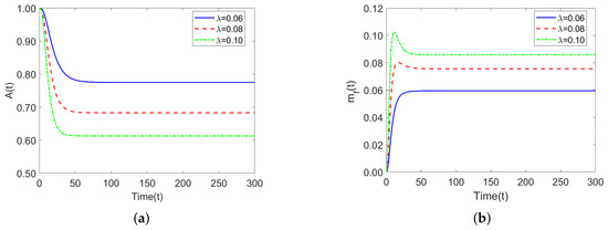
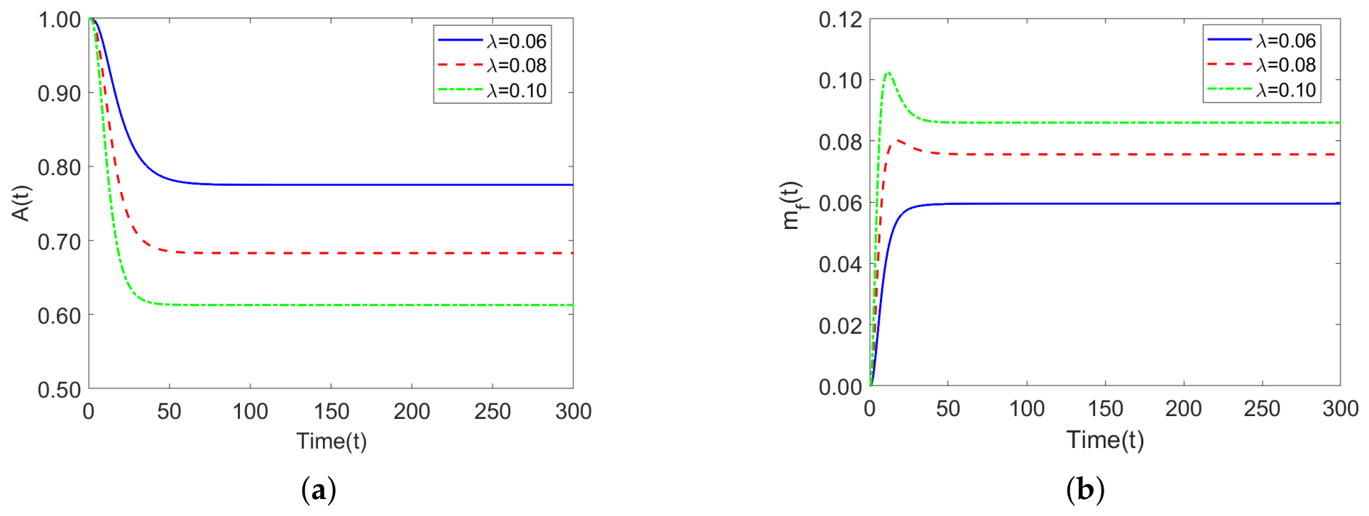
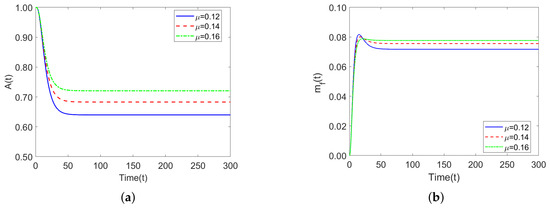
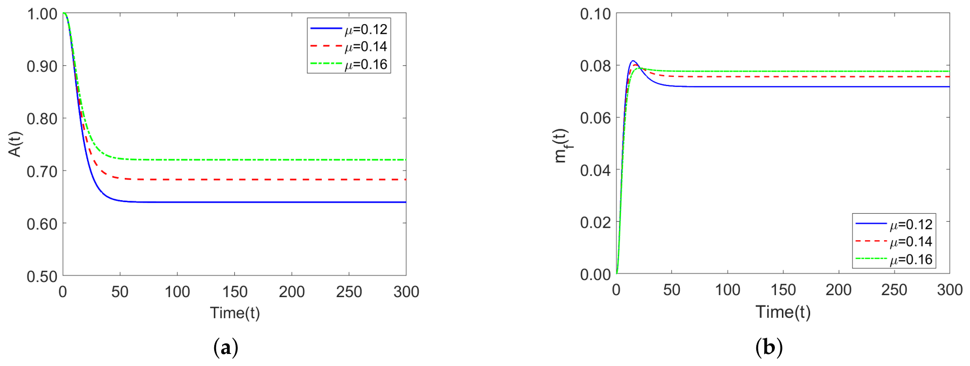
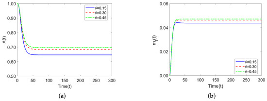
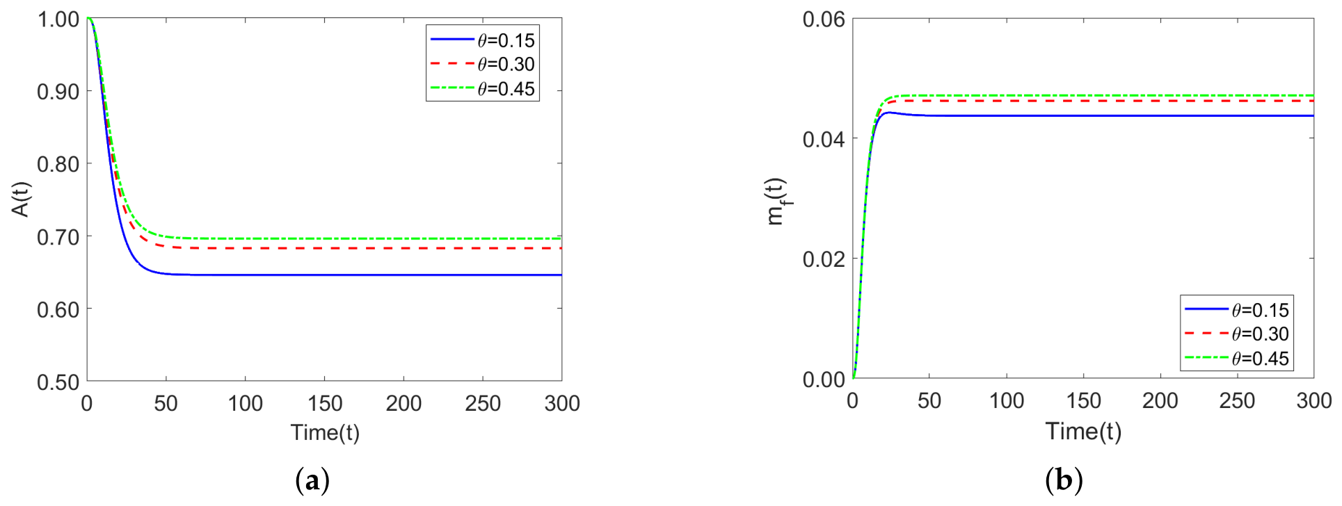
Figure 2a shows the transient availability of the system over time for different values of $\lambda$. At the initial time, the transient availability satisfies $A\left(t\right)=1$. As time increases, $A\left(t\right)$ decreases rapidly and gradually converges to a steady-state value. In addition, the transient availability decreases as $\lambda$ increases. Figure 2b shows the transient failure frequency of the system over time for different values of $\lambda$. The transient failure frequency $m_f\left(t\right)$ increases rapidly from zero, reaches a peak, and then decreases slightly before converging to a steady-state value. Moreover, $m_f\left(t\right)$ increases slightly as $\lambda$ increases.

Figure 2. Effect of parameter $\lambda$ on instantaneous reliability indices of the system. (a) Instantaneous availability, (b) Instantaneous failure frequency.

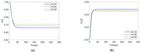
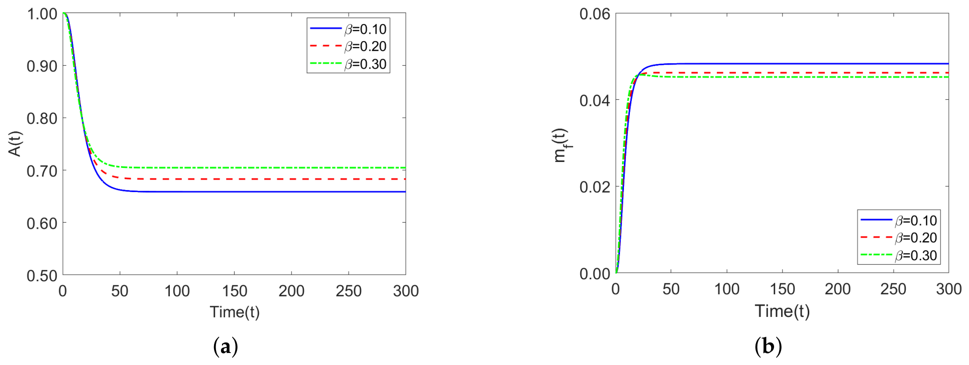
Figure 3a shows the transient availability of the system over time for different values of $\mu$. The transient availability starts from $A\left(t\right)=1$, decreases rapidly with time, and then gradually converges to a steady-state value. As $\mu$ increases, the transient availability $A\left(t\right)$ increases. Figure 3b shows the transient failure frequency of the system over time for different values of $\mu$. The transient failure frequency $m_f\left(t\right)$ rises rapidly from zero, reaches a peak, and subsequently converges to a steady-state value. As $\mu$ increases, $m_f\left(t\right)$ increases slightly.

Figure 3. Effect of parameter $\mu$ on instantaneous reliability indices of the system. (a) Instantaneous availability, (b) Instantaneous failure frequency.

Figure 4a shows the transient availability of the system over time for different values of $\beta$. As time increases, the transient availability $A\left(t\right)$ decreases rapidly from its initial value of one and then gradually approaches a steady-state value. The transient availability increases as $\beta$ increases. Figure 4b shows the transient failure frequency of the system over time for different values of $\beta$. The transient failure frequency $m_f\left(t\right)$ increases rapidly from zero and eventually converges to a constant steady-state value. As $\beta$ increases, $m_f\left(t\right)$ decreases slightly.

Figure 4. Effect of parameter $\beta$ on instantaneous reliability indices of the system. (a) Instantaneous availability, (b) Instantaneous failure frequency.

Figure 5a shows the transient availability of the system over time for different values of $\theta$. As time increases, the transient availability $A\left(t\right)$ decreases rapidly from its initial value of one and then gradually converges to a steady-state value. The transient availability increases as $\theta$ increases. Figure 5b shows the transient failure frequency of the system over time for different values of $\theta$. The transient failure frequency $m_f\left(t\right)$ increases rapidly from zero and eventually converges to a constant steady-state value. As $\theta$ increases, $m_f\left(t\right)$ increases slightly.

Figure 5. Effect of parameter $\theta$ on instantaneous reliability indices of the system. (a) Instantaneous availability, (b) Instantaneous failure frequency.

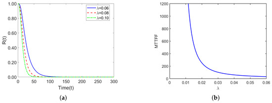
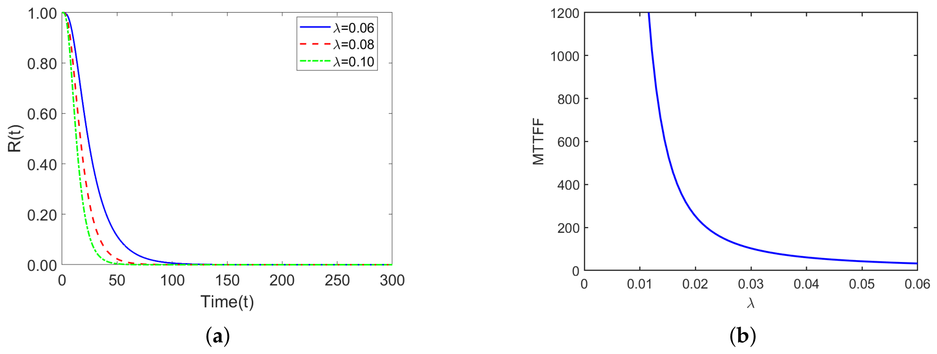
Figure 6a illustrates the effect of different values of $\lambda$ on the system reliability. The system reliability decreases monotonically over time starting from an initial value of 1 and eventually approaches 0. A larger $\lambda$ yields a faster decline of the reliability curve. Figure 6b shows how MTTFF varies with $\lambda$; MTTFF decreases as $\lambda$ increases.

Figure 6. (a) Variation of reliability function over time, (b) Variation of mean time to first failure (MTTFF) with parameter $\lambda$.

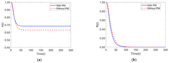
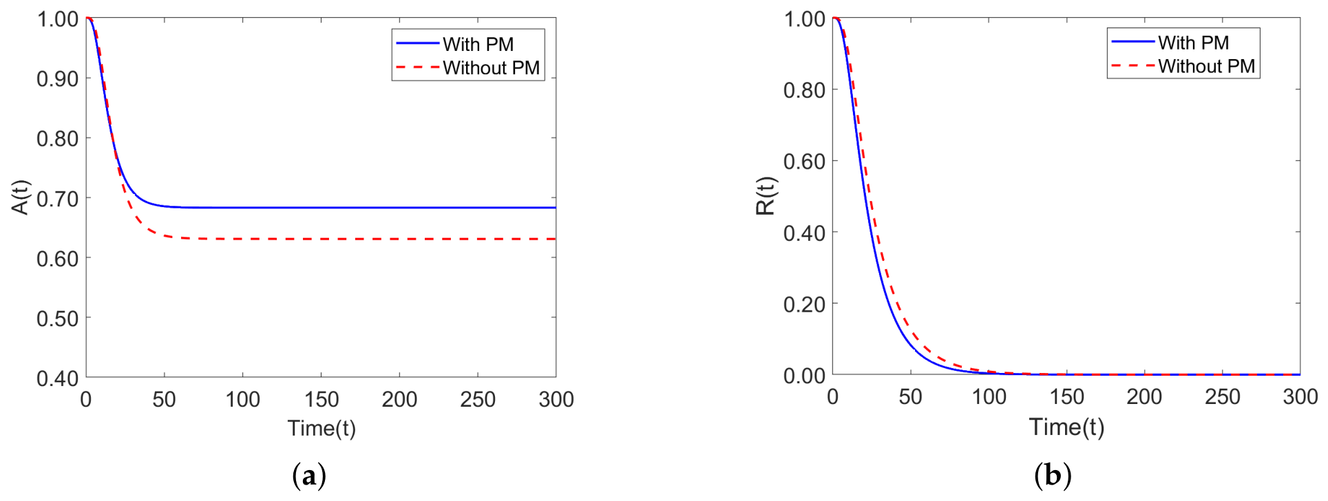
Figure 7a shows the variation of the instantaneous availability over time for the systems with and without preventive maintenance. The instantaneous availability of both systems decreases rapidly from an initial value of 1 and then gradually approaches a steady-state value. The system with preventive maintenance exhibits a higher steady-state availability than that without preventive maintenance. Figure 7b shows the variation of the reliability function over time. The reliability of both systems decreases monotonically from 1 and eventually approaches 0.

Figure 7. Variation of reliability function over time. (a) Instantaneous availability, (b) Variation of reliability function over time.

6. Conclusions

This study establishes a functional-analytic framework for a 2-out-of-6:G repairable system with preventive maintenance and investigates its dynamic behavior. The main findings are summarized as follows.

First, the supplementary variable method is applied to formulate the system, and the resulting model is represented as an abstract Cauchy problem in a Banach space.

Second, $C_0$-semigroup theory establishes that the system operator is the generator of a positive contraction $C_0$-semigroup. Accordingly, a unique nonnegative solution exists and conserves total probability.

Third, zero is established as an eigenvalue of geometric multiplicity one for both the system operator and its adjoint. Greiner’s boundary perturbation method further shows that every nonzero point on the imaginary axis belongs to the resolvent set of the system operator. This spectral property consequently implies strong convergence of the solution to the corresponding steady-state solution.

Fourth, numerical experiments illustrate the effects of model parameters on the instantaneous reliability indices. The numerical findings are consistent with the theoretical analysis.

Future studies may examine whether convergence to the steady-state solution is exponential.

References

- Barlow, R.; Hunter, L. Optimum preventive maintenance policies. Oper. Res. 1960, 8, 90–100. [Google Scholar] [CrossRef] [Scilit]
- Gaver, D. Time to failure and availability of paralleled systems with repair. IEEE Trans. Reliab. 1963, 12, 30–38. [Google Scholar] [CrossRef] [Scilit]
- Nakagawa, T. Optimum policies when preventive maintenance is imperfect. IEEE Trans. Reliab. 1979, R-28, 331–332. [Google Scholar] [CrossRef] [Scilit]
- Goel, L.R.; Sharma, G.; Gupta, P.P. Reliability analysis of a system with preventive maintenance, inspection and 2 types of repair. Microelectron. Reliab. 1986, 26, 429–433. [Google Scholar] [CrossRef] [Scilit]
- Zhang, T.L.; Horigome, M. Availability of 3-out-of-4:G warm standby system. IEICE Trans. Fundam. Electron. Comput. Sci. 2000, E83A, 857–862. [Google Scholar]
- Zheng, R.; Wu, K.; Lu, S.; Li, M. Optimal condition-based replacement policy with unknown degradation parameters. Reliab. Eng. Syst. Saf. 2025, 264, 111288. [Google Scholar] [CrossRef] [Scilit]
- Haggag, M.Y. Cost analysis of two-dissimilar-unit cold standby system with three states and preventive maintenance using linear first order differential equations. J. Math. Stat. 2009, 5, 395–400. [Google Scholar] [CrossRef] [Scilit]
- Mahmoud, M.A.W.; Moshref, M.E. On a two-unit cold standby system considering hardware, human error failures and preventive maintenance. Math. Comput. Model. 2010, 51, 736–745. [Google Scholar] [CrossRef] [Scilit]
- Dwyer, V.M. Reliability of various 2-out-of-4:G redundant systems with minimal repair. IEEE Trans. Reliab. 2012, 61, 170–179. [Google Scholar] [CrossRef] [Scilit]
- Yusuf, I.; Gimba, B. Modeling and evaluation of MTSF of 2-out-of-5 warm standby repairable system with replacement at common cause failure. Appl. Math. Sci. 2013, 7, 6403–6415. [Google Scholar] [CrossRef] [Scilit]
- Zheng, R.; Zhao, T.; Xing, Y.; Wang, X. Optimal condition-based maintenance policy under uncertain environments. Reliab. Eng. Syst. Saf. 2026, 272, 112322. [Google Scholar] [CrossRef] [Scilit]
- Xanthopoulos, A.S.; Koulouriotis, D.E.; Botsaris, P.N. Single-stage Kanban system with deterioration failures and condition-based preventive maintenance. Reliab. Eng. Syst. Saf. 2015, 142, 111–122. [Google Scholar] [CrossRef] [Scilit]
- Ali, U.A.; Bala, S.I.; Yusuf, I. Evaluation of mean time to system failure of a repairable 3-out-of-4 system with online preventive maintenance. Am. J. Appl. Math. Stat. 2014, 2, 29–33. [Google Scholar] [CrossRef] [Scilit][Green Version]
- Anuradha; Malik, S.C. Reliability measures of a 2-out-of-3: G system with priority and failure of service facility during repair. Reliab. Theory Appl. 2023, 18, 214–223. [Google Scholar]
- Yusuf, I. Reliability modelling of a parallel system with a supporting device and two types of preventive maintenance. Int. J. Oper. Res. 2016, 25, 269–287. [Google Scholar] [CrossRef] [Scilit]
- Yusuf, I.; Yusuf, B.; Suleiman, K. Reliability assessment of a repairable system under online and offline preventive maintenance. Life Cycle Reliab. Saf. Eng. 2019, 8, 391–406. [Google Scholar] [CrossRef] [Scilit]
- Zheng, R.; Ma, Y.; Zhou, Y. An optimal sampling-inspection policy for a partially observable production process. Int. J. Prod. Res. 2026, 64, 8444–8458. [Google Scholar] [CrossRef] [Scilit]
- Sultan, K.S.; Moshref, M.E.; Emiliano, C. Stochastic analysis of a priority standby system under preventive maintenance. Appl. Sci. 2021, 11, 3861. [Google Scholar] [CrossRef] [Scilit]
- Zhang, L.; Guo, L.; Li, R.; Wang, Y. A method for safety evaluation of train braking system considering multiple types of preventive maintenance cycles. Appl. Sci. 2022, 12, 4799. [Google Scholar] [CrossRef] [Scilit]
- Wang, J.; Zhang, J.; Wu, J.; Zhang, Q.; Fang, Y.; Huang, X. Optimal inspection-based maintenance strategy for k-out-of-n:G load-sharing systems consisting of three-state components. Comput. Ind. Eng. 2025, 209, 111446. [Google Scholar] [CrossRef] [Scilit]
- Liu, Y.; Wang, G.; Liu, P. A condition-based maintenance policy with non-periodic inspection for k-out-of-n: G systems. Reliab. Eng. Syst. Saf. 2024, 241, 109640. [Google Scholar] [CrossRef] [Scilit]
- Li, J.; Hu, L.; Wang, Y.; Kang, J. Reliability analysis and optimization design of a repairable k-out-of-n retrial system with two failure modes and preventive maintenance. Commun. Stat.—Theory Methods 2024, 53, 5524–5552. [Google Scholar] [CrossRef] [Scilit]
- Qi, F.; Yang, H.; Wei, L.; Shu, X. Preventive maintenance policy optimization for a weighted k-out-of-n: G system using the survival signature. Reliab. Eng. Syst. Saf. 2024, 249, 110247. [Google Scholar] [CrossRef] [Scilit]
- Ning, R.; Wang, X.; Zhao, X.; Li, Z. Joint optimization of preventive maintenance and triggering mechanism for k-out-of-n: F systems with protective devices based on periodic inspection. Reliab. Eng. Syst. Saf. 2024, 251, 110396. [Google Scholar] [CrossRef] [Scilit]
- Gupur, G. Well-posedness of a system consisting of two repairable units. Acta Anal. Funct. Appl. 2001, 3, 188–192. [Google Scholar]
- Cox, D.R. The analysis of non-Markovian stochastic processes by the inclusion of supplementary variables. Math. Proc. Camb. Philos. Soc. 1955, 51, 433–441. [Google Scholar] [CrossRef] [Scilit]
- Gupur, G. Asymptotic stability of the solution of a reliability model. Acta Anal. Funct. Appl. 2005, 7, 299–316. [Google Scholar]
- Kasim, E.; Gupur, G. Dynamic analysis of a complex system under preemptive repeat repair discipline. Bound. Value Probl. 2020, 2020, 71. [Google Scholar] [CrossRef] [Scilit]
- Haji, A.; Radl, A.A. A semigroup approach to the Gnedenko system with single vacation of a repairman. Semigroup Forum 2013, 86, 41–58. [Google Scholar] [CrossRef] [Scilit]
- Lai, C.; Eskar, R.; Kasim, E. Analysis of a k/n(G) retrial system with multiple working vacations. Axioms 2025, 14, 853. [Google Scholar] [CrossRef] [Scilit]
- Fu, C.; Kasim, E. Reliability analysis for a standby repairable system with partial failure and priority. OPSEARCH 2025. [Google Scholar] [CrossRef] [Scilit]
- Gupur, G. Functional Analysis Methods for Reliability Models; Springer Science & Business Media: Berlin/Heidelberg, Germany, 2011. [Google Scholar]
- Greiner, G. Perturbing the boundary conditions of a generator. Houst. J. Math. 1987, 13, 213–229. [Google Scholar]
- Adams, R.A.; Fournier, J.J. Sobolev Spaces; Elsevier: Amsterdam, The Netherlands, 2003. [Google Scholar]
- Fattorini, H.O. The Cauchy Problem; Cambridge University Press: Cambridge, UK, 1983. [Google Scholar]
- Gupur, G. Mathematical Methods in Reliability Theory; Science Press: Beijing, China, 2020. [Google Scholar]
Disclaimer/Publisher’s Note: The statements, opinions and data contained in all publications are solely those of the individual author(s) and contributor(s) and not of MDPI and/or the editor(s). MDPI and/or the editor(s) disclaim responsibility for any injury to people or property resulting from any ideas, methods, instructions or products referred to in the content. |
© 2026 by the authors. Licensee MDPI, Basel, Switzerland. This article is an open access article distributed under the terms and conditions of the Creative Commons Attribution (CC BY) license.