Piston Problem in Common-Velocity Idealized Three-Component Models

Abstract

This paper studies the common-velocity idealized three-component compressible model with pressure law P = ρ^γ (0 < γ ≤ 1) and the constant-pressure model with P = 1. We systematically analyze the piston problem for these two models. When the piston velocity is lower than the initial fluid velocity, fluid blockage or severe blockage occurs, corresponding to a shock or delta shock wave solution. When the piston velocity exceeds the initial fluid velocity, the flow expands, corresponding to a rarefaction wave or vacuum solution. Furthermore, we prove that, as γ → 0⁺, the conservative variables (l,m,q,ρu) of the solutions to the piston problem for the compressible model converge in the sense of distributions to those for the constant-pressure model, and we present numerical simulations for finite values of γ.

1. Introduction

Multi-component and multiphase flow phenomena are common in engineering applications such as energy transport, chemical reactors, high-pressure injections, and fluid machinery. Multi-component flow models are a key class of hyperbolic conservation laws that describe the co-transport of different material components. Based on specific physical assumptions, these models describe mass transport and momentum propagation in multi-component media at the macroscopic scale, providing a rigorous mathematical framework for investigating nonlinear wave phenomena including shock waves, rarefaction waves, contact discontinuities, vacuum states, and mass concentrations.

Real-world multiphase flows typically involve complex physical mechanisms, such as interphase relative slip, mass and momentum exchange across interfaces, viscous dissipation, wall friction, and intricate equations of state. To keep the analysis tractable, this paper does not attempt to describe all these mechanisms; instead, it focuses on a common-velocity idealized three-component model. In this model, the three components share a single velocity. At the same time, the model neglects interphase relative slip, interfacial exchanges, and wall friction, leading to passive transport of the component fractions. The one-dimensional governing equations are given by [1]:

$$\left\{\begin{array}{c}{\left({\alpha }_1{\varrho }_1\right)}_t+{\left({\alpha }_1{\varrho }_{1}u\right)}_x=0,\hfill \\ {\left({\alpha }_2{\varrho }_2\right)}_t+{\left({\alpha }_2{\varrho }_{2}u\right)}_x=0,\hfill \\ {\left({\alpha }_3{\varrho }_3\right)}_t+{\left({\alpha }_3{\varrho }_{3}u\right)}_x=0,\hfill \\ {\left(({\alpha }_1{\varrho }_1+{\alpha }_2{\varrho }_2+{\alpha }_3{\varrho }_3)u\right)}_t+{\left(({\alpha }_1{\varrho }_1+{\alpha }_2{\varrho }_2+{\alpha }_3{\varrho }_3)u^2+P\right)}_x=0,\hfill \end{array}\right.$$

(1)

where ${\alpha }_k>0$ and ${\varrho }_k>0$ represent, respectively, the volume fraction and density of the k-th component ($k=1,2,3$), satisfying ${\alpha }_1+{\alpha }_2+{\alpha }_3=1$; u denotes the common velocity of the three components; and

$$P={\rho }^{\gamma },0<\gamma \le 1,$$

(2)

represents pressure, where $\gamma$ is the equation-of-state exponent, and $\rho ={\alpha }_1{\varrho }_1+{\alpha }_2{\varrho }_2+{\alpha }_3{\varrho }_3$. For convenience in representing component and total masses, let $l={\alpha }_1{\varrho }_1,m={\alpha }_2{\varrho }_2$, and $q={\alpha }_3{\varrho }_3$. As the equation-of-state exponent $\gamma \to 0^{+}$, we obtain the constant-pressure common-velocity idealized three-component model:

$$\left\{\begin{array}{c}{l}_t+{\left(lu\right)}_x=0,\hfill \\ m_t+{\left(mu\right)}_x=0,\hfill \\ q_t+{\left(qu\right)}_x=0,\hfill \\ {\left((l+m+q)u\right)}_t+{\left((l+m+q)u^2+1\right)}_x=0.\hfill \end{array}\right.$$

(3)

In multiphase flow research, researchers have extensively studied two-phase flow models, laying the theoretical and methodological foundations for three-phase flow theory. In 1999, Saurel and Abgrall [2] proposed a two-phase compressible flow model and solution method. In 2004, Andrianov and Warnecke [3] studied the Riemann problem for the Baer–Nunziato two-phase flow model and obtained Riemann solutions. In 2017, Johansen and Liu [4] investigated the Riemann problem for hyperbolic conservation law systems of two-phase flow with general stream-tube geometries, focusing on how variations in flow-tube cross-sections affect flow evolution. In 2022, Wei and Sun [5] studied the Riemann problem for a simplified two-phase flow model with Chaplygin gas under external forces, obtained Riemann solutions, and presented numerical simulations. Research on three-phase flow has also gradually advanced. In 2023, Daude et al. [1] proposed a barotropic three-component hyperbolic conservation model, developed an HLLC Riemann solver, and validated the model and method through numerical simulations. In 2024, Jiang and Shen [6] studied the Riemann problem for an isothermal three-component model, obtained Riemann solutions, and found vacuum and delta shock wave solutions in the vanishing-pressure limit. In 2026, Jiang and Shen [7] investigated the Riemann problem for a one-dimensional ideal isentropic three-component model, revealing that as $\gamma$ approaches 1, Riemann solutions converge to delta shock wave solutions or vacuum solutions. In addition, systematic investigations of delta shock waves and measure-valued solutions arising from multiphase and pressureless flow systems have been well documented in the literature [8,9,10]. For more research results on multiphase flow models, see [11,12,13,14,15].

In bounded flow channels or transport pipelines, physical processes such as sudden valve closures, localized flow restrictions, or external mechanical compressions can be modeled as initial-boundary value problems driven by moving boundaries. As a canonical configuration in hyperbolic conservation laws, the piston problem imposes strict kinematic constraints on the moving boundary, enabling analysis of the generation and evolution of nonlinear waves (such as shock waves and rarefaction waves) and the mathematical structure of solutions. Embedding the common-velocity idealized three-component model into this piston-driven framework allows us to rigorously track the accumulation and attenuation of component masses near the boundary, thereby offering a fundamental theoretical perspective on the evolution mechanism of flow disturbances in multi-component pipeline systems.

As continuum media modeling has evolved, theoretical investigations into the piston problem have progressively deepened. In 1948, Courant and Friedrichs [16] characterized the types, existence, and mathematical structure of solutions to the piston problem, laying the theoretical foundation. In 1978, Liu [17] studied the one-dimensional free-piston problem for the classical compressible Euler equations and proved the existence of global weak solutions. In 1996, Slemrod [18] proved the existence of solutions to the piston problem for spherically symmetric isentropic compressible flows using self-similar viscous limit methods. In 2005, Wang [19] proved the global existence of shock wave solutions to the piston problem for the one-dimensional isentropic Euler equations. In 2017, Ding and Li [20] proved the stability of rarefaction wave solutions to the piston problem for the relativistic Euler equations. In 2020, Qu and Yuan [21] studied the piston problem for the Chaplygin gas Euler equations and obtained Radon measure solutions. In 2024, Wang, Guo, and Wei [22] studied the piston problem for the pressureless hydrodynamic traffic flow model and constructed shock waves, rarefaction waves, delta shock waves, and vacuum solutions. In the same year, Huang, Wang, and Shao [23] studied the piston problem for compressible flows of the generalized Chaplygin gas and proved the global existence of solutions when the piston advances or recedes at a constant speed. For further results concerning piston problems, see [24,25,26,27,28].

Let the piston trajectory be $x=x\left(t\right)$ with initial position $x\left(0\right)=0$, and suppose the fluid initially occupies the region $x<0$, with initial fluid state:

$$(l,m,q,u)(x,0)=(l_0,m_0,q_0,u_0).$$

(4)

The piston moves with the prescribed constant velocity

$$x^{\prime }\left(t\right)=s_0.$$

Whenever the fluid state at the piston is non-vacuum, the kinematic compatibility condition is

$$u(x{\left(t\right)}^{-},t)=s_0.$$

(5)

In a vacuum region, however, the conservative variables satisfy $l=m=q=\rho u=0$, and the primitive velocity u cannot be uniquely recovered from the conservative state. Therefore, when the piston is adjacent to vacuum, $x^{\prime }\left(t\right)=s_0$ specifies the velocity of the moving boundary and should not be interpreted as prescribing a uniquely determined fluid velocity inside the vacuum. For the measure-valued $\delta$-shock considered in Section 3, the corresponding kinematic condition is represented by the singular-layer velocity $u_{\mathrm{\Gamma }}=s_0$. The existence domain of the piston problem solution is:

$$\mathrm{\Omega }:=\left\{(x,t)\right|x<s_{0}t,t>0\}.$$

(6)

Most existing theories of piston problems focus only on single-component fluids. While prior works analyze two-component Riemann problems and vanishing-pressure asymptotics, piston boundary-value problems have not been extended to common-velocity idealized three-component systems, and complete wave-structure derivations for piston-driven three-component flows remain absent. Therefore, existing theories cannot clarify the internal evolution mechanism of flow disturbances in multicomponent flows.

For the common-velocity idealized three-component piston problem in the limit $\gamma \to 0$, to the best of our knowledge, a rigorous mathematical proof regarding the asymptotic relationship has not been previously established. The existing literature has not fully characterized the limiting convergence behavior of solutions to three-component piston problems.

This paper investigates piston problems for common-velocity idealized three-component models, addressing the limitation of existing theories that only cover single-component fluids [19,20,21,23]. We rigorously derive weak solutions including shock waves, rarefaction waves, delta shock waves, and vacuum states. Furthermore, we characterize the accumulation and attenuation laws of the three conserved components, providing a clear theoretical explanation of the compressive blockage and rarefaction attenuation phenomena in multicomponent flow systems. On this basis, we prove that, as the equation-of-state exponent $\gamma \to 0^{+}$, the conservative variables $(l,m,q,\rho u)$ of the solutions to the piston problem for the compressible model converge in the sense of distributions to those for the constant-pressure model, establishing a rigorous mathematical connection between these two models. In addition, we perform numerical simulations for several finite values of $\gamma$ to examine whether the observed numerical trends are consistent with the analytically established asymptotic behavior. This work enriches the theoretical system of three-component piston problems and enhances the applicability and reliability of the corresponding model theories.

To validate our theoretical results, reliable numerical methods are essential, as Noorizadegan et al. [29] recently emphasized for flow-related partial differential equations. For our numerical simulations, we adopt the HLL scheme for discretization. This numerical method has been widely applied to analyze piston flows [1,6,7,22]. The numerical results provide quantitative evidence consistent with the analytical asymptotic behavior.

In this paper, we mainly investigate the piston problem for common-velocity idealized three-component models. First, we analyze the piston problem for the compressible common-velocity idealized three-component model (1) and (2) under the boundary conditions (4)–(6). The main results are summarized in the following theorem:

Theorem 1.

Assuming the piston moves uniformly with velocity $x^{\prime }\left(t\right)=s_0$, the solution to the piston problem for the compressible common-velocity idealized three-component model (1) and (2) and (4)–(6) is given as follows:

(1) If $s_0<u_0$, there exists a shock wave solution

$$(l,m,q,u)(x,t)=\left\{\begin{array}{cc}(l_0,m_0,q_0,u_0),\hfill & \hfill -\infty <x<\sigma t,\\ (l_1,m_1,q_1,s_0),\hfill & \hfill \sigma t\le x\le s_{0}t,\end{array}\right.$$

(7)

where σ represents the shock wave speed, satisfying $l_1>l_0$, $m_1>m_0$, and $q_1>q_0$.

(2) If $u_0<s_0$, there exists a rarefaction wave solution

$$(l,m,q,u)(x,t)=\left\{\begin{array}{cc}(l_0,m_0,q_0,u_0),\hfill & \hfill -\infty <{\displaystyle \frac{x}{t}}\le {\xi }_1(l_0,m_0,q_0,u_0),\\ (l,m,q,u),\hfill & \hfill {\xi }_1(l_0,m_0,q_0,u_0)<{\displaystyle \frac{x}{t}}<{\xi }_1(l_1,m_1,q_1,s_0),\\ (l_1,m_1,q_1,s_0),\hfill & \hfill {\xi }_1(l_1,m_1,q_1,s_0)\le {\displaystyle \frac{x}{t}}\le s_0,\end{array}\right.$$

(8)

where $0<l_1<l_0$, $0<m_1<m_0$, $0<q_1<q_0$, and the state variables $(l,m,q,u)$ satisfy

$$\left\{\begin{array}{cc}u+{\displaystyle \frac{2\sqrt{\gamma {\rho }^{\gamma -1}}}{\gamma -1}}=u_0+{\displaystyle \frac{2\sqrt{\gamma {\rho }_0^{\gamma -1}}}{\gamma -1}},\hfill & \hfill 0<\gamma <1,\\ u+\ln \rho =u_0+\ln {\rho }_0,\hfill & \hfill \gamma =1,\end{array}\right.$$

with ${\displaystyle \frac{l}{l_0}}={\displaystyle \frac{m}{m_0}}={\displaystyle \frac{q}{q_0}}$ and ${\xi }_1=u-\sqrt{\gamma {\rho }^{\gamma -1}}$.

Second, we address the piston problem for the constant-pressure common-velocity idealized three-component model (3)–(6):

Theorem 2.

Assuming the piston moves uniformly with velocity $x^{\prime }\left(t\right)=s_0$, the solution to the piston problem for the constant-pressure common-velocity idealized three-component model (3)–(6) is given as follows:

(1) If $s_0<u_0$, there exists a delta shock wave solution

$$(l,m,q,u)(x,t)=\left\{\begin{array}{cc}(l_0,m_0,q_0,u_0),\hfill & \hfill -\infty <x<s_{0}t,\\ (w_1\left(t\right)\delta (x-s_{0}t),w_2\left(t\right)\delta (x-s_{0}t),w_3\left(t\right)\delta (x-s_{0}t),s_0),\hfill & \hfill x=s_{0}t,\end{array}\right.$$

(9)

where $\delta (·)$ is the delta function, and $w_1\left(t\right)=l_0(u_0-s_0)t$, $w_2\left(t\right)=m_0(u_0-s_0)t$, and $w_3\left(t\right)=q_0(u_0-s_0)t$ are the weight functions corresponding to component densities $l,m,$ and q, respectively.

(2) If $u_0<s_0$, there exists a vacuum solution

$$(l,m,q,\rho u)(x,t)=\left\{\begin{array}{cc}(l_0,m_0,q_0,{\rho }_0{u}_0),\hfill & \hfill -\infty <x<u_{0}t,\\ (0,0,0,0),\hfill & \hfill u_{0}t\le x\le s_{0}t.\end{array}\right.$$

(10)

Finally, as $\gamma \to 0$, we rigorously establish the asymptotic convergence of the solutions:

Theorem 3.

Assuming the piston moves uniformly with velocity $x^{\prime }\left(t\right)=s_0$, as $\gamma \to 0^{+}$, for each fixed $t>0$, the conservative variables $(l,m,q,\rho u)$ of the solution to the piston problem for the compressible common-velocity idealized three-component model (1) and (2) and (4)–(6) converge in the sense of distributions to the corresponding conservative variables of the solution to the piston problem for the constant-pressure common-velocity idealized three-component model (3)–(6).

This paper is structured as follows: In Section 2, we investigate the piston problem for the compressible common-velocity idealized three-component model. In Section 3, we solve the piston problem for the constant-pressure common-velocity idealized three-component model. In Section 4, we prove that, as $\gamma \to 0^{+}$, the conservative variables $(l,m,q,\rho u)$ of the compressible solutions converge in the sense of distributions to those of the constant-pressure solutions. In Section 5, we use the HLL scheme to perform numerical simulations for several finite values of $\gamma$. These computations provide quantitative evidence consistent with the asymptotic behavior established analytically in Section 4.

2. The Piston Problem for the Compressible Common-Velocity Idealized Three-Component Model

In this section, we mainly consider the piston problem for the compressible common-velocity idealized three-component model (1) and (2) and (4)–(6). Assuming the piston moves at constant velocity $x^{\prime }\left(t\right)=s_0$, based on the relative magnitude of piston velocity and initial fluid velocity, we consider the following two cases:

Case 1: $s_0<u_0$; Case 2: $u_0<s_0$.

When $s_0=u_0$, the piston moves with exactly the same velocity as the initial fluid. Consequently, no compression or rarefaction occurs in the flow field. The solution is simply the constant state $(l_0,m_0,q_0,u_0)$ for all $x<s_{0}t$ (or equivalently $x<u_{0}t$), and no shock or rarefaction wave is generated.

2.1. Case 1: $s_0<u_0$

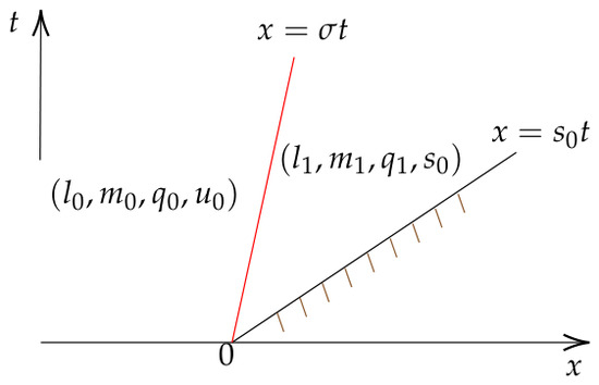
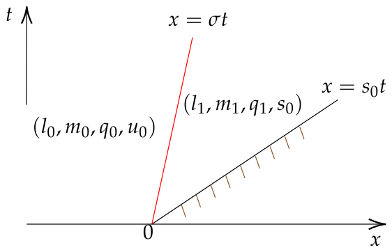
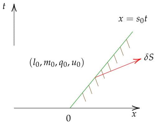
When $s_0<u_0$, i.e., the piston velocity is less than the initial fluid velocity, fluid blockage occurs in the flow field. In this case, we construct a shock wave solution (see Figure 1),

$$(l,m,q,u)(x,t)=\left\{\begin{array}{cc}(l_0,m_0,q_0,u_0),\hfill & \hfill -\infty \le x<\sigma t,\\ (l_1,m_1,q_1,s_0),\hfill & \hfill \sigma t\le x\le s_{0}t,\end{array}\right.$$

(11)

where $l_1>l_0$, $m_1>m_0$, $q_1>q_0$.

Figure 1. Solution corresponding to fluid blockage phenomenon.

Lemma 1.

If the piston moves uniformly with $x^{\prime }\left(t\right)=s_0$ and satisfies $s_0<u_0$, then the piston problem for the compressible common-velocity idealized three-component model (1) and (2) and (4)–(6) admits a shock wave solution (7) satisfying $l_1>l_0$, $m_1>m_0$, $q_1>q_0$.

Proof. 

According to the system of equations and initial conditions, the Rankine–Hugoniot conditions are

$$\left\{\begin{array}{c}\sigma (l_1-l_0)=l_1{s}_0-l_0{u}_0,\hfill \\ \sigma (m_1-m_0)=m_1{s}_0-m_0{u}_0,\hfill \\ \sigma (q_1-q_0)=q_1{s}_0-q_0{u}_0,\hfill \\ \sigma ({\rho }_1{s}_0-{\rho }_0{u}_0)={\rho }_1{s}_0^2-{\rho }_0{u}_0^2+{\rho }_1^{\gamma }-{\rho }_0^{\gamma },\hfill \end{array}\right.$$

(12)

where ${\rho }_0=l_0+m_0+q_0$, ${\rho }_1=l_1+m_1+q_1$. From the first, second, and third equations in (12), we deduce that

$$\sigma ={\displaystyle \frac{l_1{s}_0-l_0{u}_0}{l_1-l_0}}={\displaystyle \frac{m_1{s}_0-m_0{u}_0}{m_1-m_0}}={\displaystyle \frac{q_1{s}_0-q_0{u}_0}{q_1-q_0}}={\displaystyle \frac{{\rho }_1{s}_0-{\rho }_0{u}_0}{{\rho }_1-{\rho }_0}}.$$

(13)

Substituting (13) into the fourth equation in (12) leads to

$${\displaystyle \frac{{({\rho }_1{s}_0-{\rho }_0{u}_0)}^2}{{\rho }_1-{\rho }_0}}={\rho }_1{s}_0^2-{\rho }_0{u}_0^2+{\rho }_1^{\gamma }-{\rho }_0^{\gamma }.$$

(14)

From (13), we have

$$l_1={\displaystyle \frac{l_0(\sigma -u_0)}{\sigma -s_0}},m_1={\displaystyle \frac{m_0(\sigma -u_0)}{\sigma -s_0}},q_1={\displaystyle \frac{q_0(\sigma -u_0)}{\sigma -s_0}},{\rho }_1={\displaystyle \frac{{\rho }_0(\sigma -u_0)}{\sigma -s_0}}.$$

(15)

Let

$$k={\displaystyle \frac{\sigma -u_0}{\sigma -s_0}}.$$

(16)

Since we are seeking a shock wave with $l_1>l_0$, $m_1>m_0$ and $q_1>q_0$, it follows from (15) that

$${\displaystyle \frac{l_1}{l_0}}={\displaystyle \frac{m_1}{m_0}}={\displaystyle \frac{q_1}{q_0}}={\displaystyle \frac{{\rho }_1}{{\rho }_0}}=k.$$

(17)

Thus, we require $k>1$, which is precisely the compression ratio across the shock. Substituting (17) into (14) yields

$${\displaystyle \frac{{(k{s}_0-u_0)}^2{\rho }_0}{k-1}}=(k{s}_0^2-u_0^2){\rho }_0+(k^{\gamma }-1){\rho }_0^{\gamma }.$$

(18)

From (18), we have

$$k{\rho }_0{(u_0-s_0)}^2-(k-1)(k^{\gamma }-1){\rho }_0^{\gamma }=0.$$

(19)

Let

$$G_{\gamma }\left(k\right):={\displaystyle \frac{(k-1)(k^{\gamma }-1)}{k}}={\displaystyle \frac{{\rho }_0{(u_0-s_0)}^2}{{\rho }_0^{\gamma }}}.$$

(20)

Note that

$$G_{\gamma }\left(k\right)=\left(1-{\displaystyle \frac{1}{k}}\right)(k^{\gamma }-1).$$

For $k>1$, both factors $(1-{\displaystyle \frac{1}{k}})$ and $(k^{\gamma }-1)$ are positive and strictly increasing in k. Hence, $G_{\gamma }\left(k\right)$ is strictly increasing on $(1,+\infty )$. Furthermore,

$$\underset{k\to 1+}{\lim }{G}_{\gamma }\left(k\right)=0,\underset{k\to \infty }{\lim }{G}_{\gamma }\left(k\right)=+\infty .$$

Since ${\rho }_0>0$ and $u_0-s_0>0$, the right-hand side of (20) is a positive constant for each fixed $\gamma >0$. By the Intermediate Value Theorem and monotonicity, for every $\gamma >0$, there exists a unique $k\left(\gamma \right)>1$ satisfying (20). Therefore, from ${\rho }_1=k{\rho }_0$, we obtain the unique physical solution satisfying $l_1=k{l}_0>l_0$, $m_1=k{m}_0>m_0$, and $q_1=k{q}_0>q_0$.

We now show that the shock speed satisfies $\sigma <s_0$. From (13), it follows that

$$\sigma -s_0={\displaystyle \frac{l_1{s}_0-l_0{u}_0}{l_1-l_0}}-s_0={\displaystyle \frac{l_0(s_0-u_0)}{l_1-l_0}}.$$

Since $s_0<u_0$ and $l_1>l_0$, we conclude that

$$\sigma -s_0<0.$$

We verify that the constructed shock satisfies the Lax entropy admissibility condition. From (13) and ${\rho }_1=k{\rho }_0$, we rewrite the shock speed as

$$\sigma =s_0-{\displaystyle \frac{u_0-s_0}{k-1}}.$$

Substituting the above expression of $\sigma$ into $s_0-c_1<\sigma$, this inequality is equivalent to

$${\displaystyle \frac{u_0-s_0}{k-1}}<c_1.$$

Combining the sound speed relation $c_1^2=\gamma {\rho }_1^{\gamma -1}$ and the implicit relation (19), we find that the above inequality is further equivalent to

$$1-k^{-\gamma }<\gamma (k-1).$$

Similarly, substituting the formula of $\sigma$ into $\sigma <u_0-c_0$ shows that this inequality is equivalent to

$$c_0<{\displaystyle \frac{k(u_0-s_0)}{k-1}}.$$

Using the sound speed relation $c_0^2=\gamma {\rho }_0^{\gamma -1}$ together with (19), the above inequality is equivalent to

$${\displaystyle \frac{k(k^{\gamma }-1)}{k-1}}>\gamma .$$

Define

$$f\left(k\right)=\gamma (k-1)-1+k^{-\gamma }.$$

It is obvious that $f\left(1\right)=0$. Direct calculation gives

$$f^{\prime }\left(k\right)=\gamma \left(1-k^{-\gamma -1}\right)>0,k>1.$$

Thus, $f\left(k\right)$ is strictly increasing for $k>1$, which implies $f\left(k\right)>0$. Consequently,

$$1-k^{-\gamma }<\gamma (k-1).$$

Define

$$g\left(k\right)=k(k^{\gamma }-1)-\gamma (k-1).$$

We have $g\left(1\right)=0$ and

$$g^{\prime }\left(k\right)=(\gamma +1)(k^{\gamma }-1)>0,k>1.$$

Hence, $g\left(k\right)$ is strictly increasing for $k>1$, so $g\left(k\right)>0$, which yields

$${\displaystyle \frac{k(k^{\gamma }-1)}{k-1}}>\gamma .$$

Combining the above estimates, we obtain the complete Lax inequalities

$${\lambda }_1\left(U_1\right)=s_0-c_1<\sigma <u_0-c_0={\lambda }_1\left(U_0\right).$$

Together with $\sigma <s_0={\lambda }_2\left(U_1\right)={\lambda }_3\left(U_1\right)$, we conclude that the constructed discontinuity is a compressive shock of the first characteristic family and satisfies the Lax entropy admissibility condition. Finally, the 4-wave family is geometrically incompatible with the piston flow configuration. A direct computation shows

$${\lambda }_4\left(U_1\right)=s_0+c_1>s_0.$$

Thus, any wave of the 4-family propagates toward the region $x>s_{0}t$, which lies outside the fluid domain $\mathrm{\Omega }$. As a result, the 4-shock structure cannot appear in the present piston problem.

Therefore, for $s_0<u_0$, we have constructed an admissible 1-shock wave solution (7) satisfying the piston problem for the compressible common-velocity idealized three-component model (1) and (2) and (4)–(6). □

2.2. Case 2: $u_0<s_0$

When $u_0<s_0$, i.e., the piston velocity exceeds the initial fluid velocity, rarefaction occurs in the flow field. From (1) and (2), we obtain

$$\left(\begin{array}{cccc}1& 0& 0& 0\\ 0& 1& 0& 0\\ 0& 0& 1& 0\\ u& u& u& \rho \end{array}\right){\left(\begin{array}{c}l\\ m\\ q\\ u\end{array}\right)}_t+\left(\begin{array}{cccc}u& 0& 0& l\\ 0& u& 0& m\\ 0& 0& u& q\\ u^2+c^2& u^2+c^2& u^2+c^2& 2u\rho \end{array}\right){\left(\begin{array}{c}l\\ m\\ q\\ u\end{array}\right)}_x=\left(\begin{array}{c}0\\ 0\\ 0\\ 0\end{array}\right),$$

(21)

where $c=\sqrt{\gamma {\rho }^{\gamma -1}}(\gamma >0)$. From (21), we obtain the eigenvalues of system (1) and (2) as

$${\lambda }_1=u-c,{\lambda }_2={\lambda }_3=u,{\lambda }_4=u+c.$$

(22)

The corresponding right eigenvectors are

$${\overrightarrow{r}}_1={\left(l,m,q,-c\right)}^T,{\overrightarrow{r}}_2={\left(1,0,-1,0\right)}^T,{\overrightarrow{r}}_3={\left(1,-1,0,0\right)}^T,{\overrightarrow{r}}_4={\left(l,m,q,c\right)}^T.$$

(23)

From (22) and (23), it follows that

$$\nabla {\lambda }_1·{\overrightarrow{r}}_1=-{\displaystyle \frac{1}{2}}(\gamma +1)\sqrt{\gamma {\rho }^{\gamma -1}}\ne 0,\nabla {\lambda }_2·{\overrightarrow{r}}_2=\nabla {\lambda }_3·{\overrightarrow{r}}_3=0,\nabla {\lambda }_4·{\overrightarrow{r}}_4={\displaystyle \frac{1}{2}}(\gamma +1)\sqrt{\gamma {\rho }^{\gamma -1}}\ne 0.$$

(24)

From (24), ${\lambda }_1$ and ${\lambda }_4$ are genuinely nonlinear, while ${\lambda }_2$ and ${\lambda }_3$ are linearly degenerate. From ${\lambda }_1=u-\sqrt{\gamma {\rho }^{\gamma -1}}$ and ${\overrightarrow{r}}_1={\left(l,m,q,-c\right)}^T$, we have

$${\displaystyle \frac{dl}{l}}={\displaystyle \frac{dm}{m}}={\displaystyle \frac{dq}{q}}={\displaystyle \frac{du}{-c}}.$$

(25)

Integrating (25) subject to the initial data (4) yields

$$\left\{\begin{array}{cc}u+{\displaystyle \frac{2\sqrt{\gamma {\rho }^{\gamma -1}}}{\gamma -1}}=u_0+{\displaystyle \frac{2\sqrt{\gamma {\rho }_0^{\gamma -1}}}{\gamma -1}},\hfill & \hfill 0<\gamma <1,\\ u+\ln \rho =u_0+\ln {\rho }_0,\hfill & \hfill \gamma =1,\end{array}\right.$$

(26)

and

$${\displaystyle \frac{l}{l_0}}={\displaystyle \frac{m}{m_0}}={\displaystyle \frac{q}{q_0}}.$$

(27)

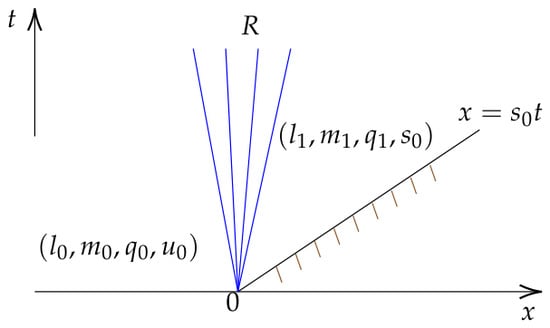
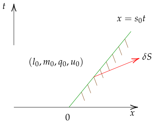
Let $\xi ={\displaystyle \frac{x}{t}}$. Using (26) and (27) together with ${\xi }_1={\lambda }_1=u-c$, we construct a rarefaction wave solution (see Figure 2),

$$(l,m,q,u)(x,t)=\left\{\begin{array}{cc}(l_0,m_0,q_0,u_0),\hfill & \hfill -\infty <{\displaystyle \frac{x}{t}}\le {\xi }_1(l_0,m_0,q_0,u_0),\\ (l,m,q,u),\hfill & \hfill {\xi }_1(l_0,m_0,q_0,u_0)<{\displaystyle \frac{x}{t}}<{\xi }_1(l_1,m_1,q_1,s_0),\\ (l_1,m_1,q_1,s_0),\hfill & \hfill {\xi }_1(l_1,m_1,q_1,s_0)\le {\displaystyle \frac{x}{t}}\le s_0,\end{array}\right.$$

(28)

where $0<l_1<l_0$, $0<m_1<m_0$, $0<q_1<q_0$, and $l,m,q,u$ satisfy (26) and (27).

Figure 2. Solution corresponding to fluid rarefaction phenomenon.

Lemma 2.

If the piston moves uniformly with $x^{\prime }\left(t\right)=s_0$ and satisfies $u_0<s_0$, then the piston problem for the compressible common-velocity idealized three-component model (1) and (2) and (4)–(6) admits a rarefaction wave solution (8), with $l_1<l_0$, $m_1<m_0$, $q_1<q_0$.

Proof. 

We need to prove that the solution (8) to the piston problem for the compressible common-velocity idealized three-component model (1) and (2) and (4)–(6) satisfies $0<{\rho }_1<{\rho }_0$ and that the characteristic speeds satisfy ${\xi }_1(l_0,m_0,q_0,u_0)<{\xi }_1(l_1,m_1,q_1,s_0)<s_0.$

First, we prove the existence of $l,m,q$ satisfying $0<l_1<l_0$, $0<m_1<m_0$, $0<q_1<q_0$. The states $(l_0,m_0,q_0,u_0)$ and $(l_1,m_1,q_1,s_0)$ satisfy

$$\left\{\begin{array}{cc}{s}_0+{\displaystyle \frac{2\sqrt{\gamma {\rho }_1^{\gamma -1}}}{\gamma -1}}=u_0+{\displaystyle \frac{2\sqrt{\gamma {\rho }_0^{\gamma -1}}}{\gamma -1}},\hfill & \hfill 0<\gamma <1,\\ s_0+\ln {\rho }_1=u_0+\ln {\rho }_0,\hfill & \hfill \gamma =1,\end{array}\right.$$

(29)

and

$${\displaystyle \frac{l_1}{l_0}}={\displaystyle \frac{m_1}{m_0}}={\displaystyle \frac{q_1}{q_0}}={\displaystyle \frac{{\rho }_1}{{\rho }_0}}.$$

(30)

From (29), we have

$$\left\{\begin{array}{cc}{\displaystyle \frac{2\sqrt{\gamma {\rho }_1^{\gamma -1}}-2\sqrt{\gamma {\rho }_0^{\gamma -1}}}{\gamma -1}}=u_0-s_0,\hfill & \hfill 0<\gamma <1,\\ \ln {\rho }_1-\ln {\rho }_0=u_0-s_0,\hfill & \hfill \gamma =1.\end{array}\right.$$

Since $u_0<s_0$, it follows that

$$0<{\rho }_1<{\rho }_0.$$

Together with (30), this implies

$$0<l_1={\displaystyle \frac{{\rho }_1}{{\rho }_0}}{l}_0<l_0.$$

Similarly,

$$0<m_1<m_0,0<q_1<q_0.$$

Second, we prove ${\xi }_1(l_0,m_0,q_0,u_0)<{\xi }_1(l_1,m_1,q_1,s_0)<s_0.$ For $0<\gamma <1$, from (29), we obtain

$$c_1-c_0={\displaystyle \frac{1-\gamma }{2}}(s_0-u_0),$$

where

$$c_i=\sqrt{\gamma {\rho }_i^{\gamma -1}},i=0,1.$$

Hence,

$$\begin{array}{cc}\hfill {\xi }_1(l_1,m_1,q_1,s_0)-{\xi }_1(l_0,m_0,q_0,u_0)& =(s_0-u_0)-(c_1-c_0)\hfill \\ & ={\displaystyle \frac{1+\gamma }{2}}(s_0-u_0)>0.\hfill \end{array}$$

For $\gamma =1$, since $c_0=c_1=1$,

$${\xi }_1(l_1,m_1,q_1,s_0)-{\xi }_1(l_0,m_0,q_0,u_0)=s_0-u_0>0.$$

From (22),

$${\xi }_1(l_1,m_1,q_1,s_0)=s_0-\sqrt{\gamma {\rho }_1^{\gamma -1}}<s_0.$$

Therefore, when $u_0<s_0$, the piston problem for the compressible common-velocity idealized three-component model (1) and (2) and (4)–(6) admits a rarefaction wave solution (8). □

Based on Lemmas 1 and 2, Theorem 1 is proved.

3. The Piston Problem for the Constant-Pressure Common-Velocity Idealized Three-Component Model

This section mainly considers the piston problem for the constant-pressure common-velocity idealized three-component model (3)–(6). Assuming the piston moves at constant velocity $x^{\prime }\left(t\right)=s_0$, based on the relative magnitude of the piston velocity and the initial fluid velocity, we consider the following two cases:

Case 1: $s_0<u_0$; Case 2: $u_0<s_0$.

When $s_0=u_0$, the piston moves with exactly the same velocity as the initial fluid. Consequently, no compression or rarefaction occurs in the flow field. The solution is simply the constant state $(l_0,m_0,q_0,u_0)$ for all $x<s_{0}t$ (or equivalently $x<u_{0}t$), and no shock or rarefaction wave is generated.

3.1. Case 1: $s_0<u_0$

When $s_0<u_0$, i.e., the piston velocity is less than the initial fluid velocity, severe blockage occurs in the flow field. From (3), we obtain

$$\left(\begin{array}{cccc}1& 0& 0& 0\\ 0& 1& 0& 0\\ 0& 0& 1& 0\\ 0& 0& 0& 1\end{array}\right){\left(\begin{array}{c}l\\ m\\ q\\ u\end{array}\right)}_t+\left(\begin{array}{cccc}u& 0& 0& l\\ 0& u& 0& m\\ 0& 0& u& q\\ 0& 0& 0& u\end{array}\right){\left(\begin{array}{c}l\\ m\\ q\\ u\end{array}\right)}_x=\left(\begin{array}{c}0\\ 0\\ 0\\ 0\end{array}\right).$$

(31)

This system admits a quadruply repeated eigenvalue ${\lambda }_1={\lambda }_2={\lambda }_3={\lambda }_4=u$, with the corresponding right eigenvector $\mathit{r}={(a_1,a_2,a_3,0)}^T$, where $a_1,a_2,a_3$ are arbitrary constants. The eigenvalue u has algebraic multiplicity four and geometric multiplicity three. Hence, the system fails to be strictly hyperbolic and is only weakly hyperbolic. When $s_0<u_0$, classical bounded weak solutions do not exist, and measure-valued solutions must be introduced.

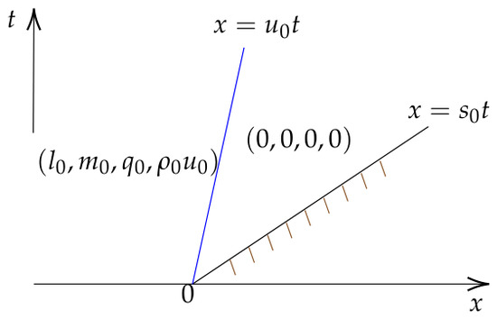
Since classical weak solutions break down and fluid mass accumulates along the piston trajectory, we introduce a delta shock solution to describe this singular flow structure (see Figure 3):

$$(l,m,q,u)(x,t)=\left\{\begin{array}{cc}(l_0,m_0,q_0,u_0),\hfill & \hfill -\infty \le x<s_{0}t,\\ (w_1\left(t\right)\delta (x-s_{0}t),w_2\left(t\right)\delta (x-s_{0}t),w_3\left(t\right)\delta (x-s_{0}t),s_0),\hfill & \hfill x=s_{0}t,\end{array}\right.$$

(32)

where $w_1\left(t\right)=l_0(u_0-s_0)t$, $w_2\left(t\right)=m_0(u_0-s_0)t$, $w_3\left(t\right)=q_0(u_0-s_0)t$.

Figure 3. Solution corresponding to severe fluid blockage phenomenon.

First, to give a mathematically rigorous formulation of the delta shock wave solution, we define the two-dimensional weighted $\delta$-function supported on a smooth curve.

Definition 1.

Let $\mathrm{\Gamma }=\{(x,t)\mid x=s_{0}t,t\ge 0\}$ be a smooth straight line of the $(x,t)$-plane. A two-dimensional weighted δ-function $w\left(t\right){\delta }_{\mathrm{\Gamma }}$ supported on Γ is defined as a distribution such that for any test function $\phi (x,t)\in C_0^{\infty }(\mathbb{R}\times [0,+\infty ))$,

$$⟨w\left(t\right){\delta }_{\mathrm{\Gamma }},\phi (x,t)⟩={\int }_0^{+\infty }w\left(t\right)\phi (s_{0}t,t)\mathrm{d}t.$$

(33)

Second, we present the definition of measure-valued weak solutions for the piston problem of the constant-pressure common-velocity idealized three-component model (3)–(6).

Definition 2.

A state $(l,m,q,u)(x,t)$ is given in the form

$$\left\{\begin{array}{cc}\hfill l(x,t)& =\widehat{l}(x,t)+w_1\left(t\right){\delta }_{\mathrm{\Gamma }},\hfill \\ \hfill m(x,t)& =\widehat{m}(x,t)+w_2\left(t\right){\delta }_{\mathrm{\Gamma }},\hfill \\ \hfill q(x,t)& =\widehat{q}(x,t)+w_3\left(t\right){\delta }_{\mathrm{\Gamma }},\hfill \\ \hfill u(x,t)& \in L^{\infty }\left(\mathrm{\Omega }\right),\hfill \end{array}\right.$$

(34)

where $\widehat{l},\widehat{m},\widehat{q}\in L^{\infty }\left(\mathrm{\Omega }\right)$ are the absolutely continuous parts, $w_i\left(t\right){\delta }_{\mathrm{\Gamma }}$$(i=1,2,3)$ are the singular (Dirac) parts of the component densities, and $u\in L^{\infty }\left(\mathrm{\Omega }\right)$ denotes the bulk fluid velocity. The singular mass concentration supported on Γ moves with the velocity

$$u_{\mathrm{\Gamma }}=s_0,$$

as follows from the piston kinematic condition. The corresponding component mass-flux distributions are defined by

$$\begin{array}{cc}\hfill lu& :=\widehat{l}u+s_0{w}_1\left(t\right){\delta }_{\mathrm{\Gamma }},\hfill \\ \hfill mu& :=\widehat{m}u+s_0{w}_2\left(t\right){\delta }_{\mathrm{\Gamma }},\hfill \\ \hfill qu& :=\widehat{q}u+s_0{w}_3\left(t\right){\delta }_{\mathrm{\Gamma }}.\hfill \end{array}$$

(35)

Here, the singular parts of the fluxes are transported with $u_{\mathrm{\Gamma }}=s_0$. This state is called a δ-shock weak solution of the piston problem (3)–(6) if and only if it satisfies the integral identities (36) for any test function $\phi \in C_0^{\infty }(\mathbb{R}\times [0,+\infty ))$:

$$\left\{\begin{array}{c}{\int \int }_{\mathrm{\Omega }}\left(\widehat{l}{\phi }_t+\widehat{l}u{\phi }_x\right)\mathrm{d}x\mathrm{d}t+{\int }_0^{+\infty }{w}_1\left(t\right)\left({\phi }_t(s_{0}t,t)+s_0{\phi }_x(s_{0}t,t)\right)\mathrm{d}t+{\int }_{-\infty }^{0}l(x,0)\phi (x,0)\mathrm{d}x=0,\hfill \\ {\int \int }_{\mathrm{\Omega }}\left(\widehat{m}{\phi }_t+\widehat{m}u{\phi }_x\right)\mathrm{d}x\mathrm{d}t+{\int }_0^{+\infty }{w}_2\left(t\right)\left({\phi }_t(s_{0}t,t)+s_0{\phi }_x(s_{0}t,t)\right)\mathrm{d}t+{\int }_{-\infty }^{0}m(x,0)\phi (x,0)\mathrm{d}x=0,\hfill \\ {\int \int }_{\mathrm{\Omega }}\left(\widehat{q}{\phi }_t+\widehat{q}u{\phi }_x\right)\mathrm{d}x\mathrm{d}t+{\int }_0^{+\infty }{w}_3\left(t\right)\left({\phi }_t(s_{0}t,t)+s_0{\phi }_x(s_{0}t,t)\right)\mathrm{d}t+{\int }_{-\infty }^{0}q(x,0)\phi (x,0)\mathrm{d}x=0,\hfill \\ {\int \int }_{\mathrm{\Omega }}\left\{(\widehat{l}+\widehat{m}+\widehat{q})u{\phi }_t+\left((\widehat{l}+\widehat{m}+\widehat{q})u^2+1\right){\phi }_x\right\}\mathrm{d}x\mathrm{d}t\hfill \\ +{\int }_0^{+\infty }(w_1\left(t\right)+w_2\left(t\right)+w_3\left(t\right))s_0\left({\phi }_t(s_{0}t,t)+s_0{\phi }_x(s_{0}t,t)\right)\mathrm{d}t\hfill \\ +{\int }_{-\infty }^0(\widehat{l}+\widehat{m}+\widehat{q})(x,0)u(x,0)\phi (x,0)\mathrm{d}x-{\int }_0^{+\infty }{F}_p\left(t\right)\phi (s_{0}t,t)\mathrm{d}t=0.\hfill \end{array}\right.$$

(36)

where $w_i\left(t\right)$$(i=1,2,3)$ denote the strength of the mass concentration for each component carried by the δ-shock along the piston trajectory Γ, and $F_p\left(t\right)$ denotes the reaction force exerted on the moving piston boundary.

Remark 1.

The singular-layer velocity $u_{\mathrm{\Gamma }}=s_0$ follows from the piston kinematic condition and represents the velocity of the mass concentration supported on Γ, whereas $u\in L^{\infty }\left(\mathrm{\Omega }\right)$ denotes the bulk fluid velocity. The boundary term involving $F_p\left(t\right)$ in the weak formulation ensures that the momentum balance is compatible with the uniform motion of the piston.

Next, we prove that the delta shock wave solution (34) is a weak solution of the piston problem for the constant-pressure three-component model (3)–(6).

Lemma 3.

If the piston moves uniformly with $x^{\prime }\left(t\right)=s_0$ and satisfies $s_0<u_0$, then the piston problem for the constant-pressure common-velocity idealized three-component model (3)–(6) admits a delta shock wave solution as given in (9).

Proof. 

From the weak solution definition (36), the first equation in (36) can be written as

$$\begin{array}{cc}\hfill 0& ={\int }_0^{+\infty }{\int }_{-\infty }^{s_{0}t}{l}_0{\phi }_t+l_0{u}_0{\phi }_{x}dxdt+{\int }_{-\infty }^0{l}_0\phi (x,0)dx\hfill \\ & +{\int }_0^{+\infty }{w}_1\left(t\right)\left\{{\phi }_t\left(s_{0}t,t\right)+s_0{\phi }_x\left(s_{0}t,t\right)\right\}dt\hfill \\ & ={\int }_0^{+\infty }{l}_0(u_0-s_0)\phi \left(s_{0}t,t\right)dt-w_1\left(0\right)\phi (0,0)\hfill \\ & -{\int }_0^{+\infty }{\displaystyle \frac{d{w}_1\left(t\right)}{dt}}\phi \left(s_{0}t,t\right)dt\hfill \\ & ={\int }_0^{+\infty }\left\{l_0(u_0-s_0)-{\displaystyle \frac{d{w}_1\left(t\right)}{dt}}\right\}\phi \left(s_{0}t,t\right)dt-w_1\left(0\right)\phi (0,0).\hfill \end{array}$$

Due to the arbitrariness of $\phi \in C_0^{\infty }(\mathbb{R}\times {\mathbb{R}}_{+})$, we have

$${\displaystyle \frac{d{w}_1\left(t\right)}{dt}}=l_0(u_0-s_0),$$

(37)

and

$$w_1\left(0\right)=0.$$

(38)

From (37) and (38), it follows that

$$w_1\left(t\right)=l_0(u_0-s_0)t\ge 0.$$

(39)

Similarly, from the second and third equations in (36), we obtain

$$w_2\left(t\right)=m_0(u_0-s_0)t\ge 0,$$

(40)

and

$$w_3\left(t\right)=q_0(u_0-s_0)t\ge 0.$$

(41)

The fourth equation in (36) can be written as

$$\begin{array}{cc}\hfill 0& ={\int }_0^{+\infty }{\int }_{-\infty }^{s_{0}t}\left\{\left(l_0+m_0+q_0\right)u_0{\phi }_t+\left(l_0+m_0+q_0\right)u_0^2{\phi }_x\right\}dxdt\hfill \\ & +{\int \int }_{\mathrm{\Omega }}{\phi }_{x}dxdt+{\int }_{-\infty }^0\left(l_0+m_0+q_0\right)u_0\phi (x,0)dx-{\int }_0^{+\infty }{F}_p\left(t\right)\phi \left(s_{0}t,t\right)dt\hfill \\ & +{\int }_0^{+\infty }(w_1\left(t\right)+w_2\left(t\right)+w_3\left(t\right))s_0\left\{{\phi }_t\left(s_{0}t,t\right)+s_0{\phi }_x\left(s_{0}t,t\right)\right\}dt\hfill \\ & ={\int }_0^{+\infty }\left(\left(l_0+m_0+q_0\right)u_0(u_0-s_0)\right)\phi \left(s_{0}t,t\right)dt+{\int }_0^{+\infty }\phi (s_{0}t,t)dt\hfill \\ & -{\int }_0^{+\infty }{s}_0\left({\displaystyle \frac{d{w}_1\left(t\right)}{dt}}+{\displaystyle \frac{d{w}_2\left(t\right)}{dt}}+{\displaystyle \frac{d{w}_3\left(t\right)}{dt}}\right)\phi \left(s_{0}t,t\right)dt-{\int }_0^{+\infty }{F}_p\left(t\right)\phi \left(s_{0}t,t\right)dt\hfill \\ & -(w_1\left(0\right)+w_2\left(0\right)+w_3\left(0\right))s_0\phi \left(0,0\right)\hfill \\ & ={\int }_0^{+\infty }\left[\left(l_0+m_0+q_0\right)u_0(u_0-s_0)-s_0\left({\displaystyle \frac{d{w}_1\left(t\right)}{dt}}+{\displaystyle \frac{d{w}_2\left(t\right)}{dt}}+{\displaystyle \frac{d{w}_3\left(t\right)}{dt}}\right)-F_p\left(t\right)+1\right]\phi \left(s_{0}t,t\right)dt\hfill \\ & -(w_1\left(0\right)+w_2\left(0\right)+w_3\left(0\right))s_0\phi \left(0,0\right),\hfill \end{array}$$

Due to the arbitrariness of $\phi$, we obtain

$$F_p\left(t\right)=(l_0+m_0+q_0)u_0\left(u_0-s_0\right)-s_0\left({\displaystyle \frac{d{w}_1\left(t\right)}{dt}}+{\displaystyle \frac{d{w}_2\left(t\right)}{dt}}+{\displaystyle \frac{d{w}_3\left(t\right)}{dt}}\right)+1.$$

From (39)–(41),

$$F_p\left(t\right)=(l_0+m_0+q_0){(u_0-s_0)}^2+1\ge 0.$$

(42)

The delta shock wave solution (9) satisfies the one-sided compressive admissibility condition $s_0<u_0$. Therefore, when $s_0<u_0$, we can construct a delta shock wave solution (9) satisfying the piston problem (3)–(6). This condition acts as the admissibility criterion, and the delta shock solution is unique within the class of solutions consisting of the constant left state and a single Dirac mass supported on $\mathrm{\Gamma }$. □

3.2. Case 2: $u_0<s_0$

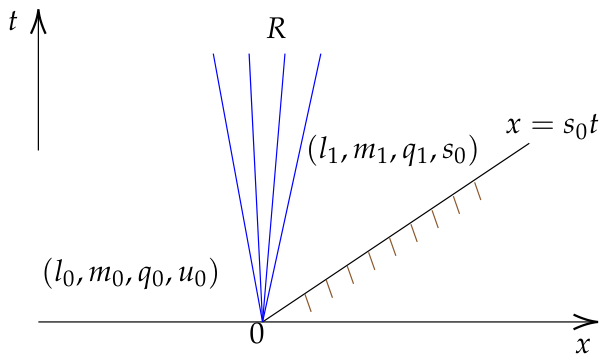
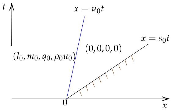
When $u_0<s_0$, i.e., the piston velocity exceeds the initial fluid velocity, a vacuum region forms in the flow field. A cavity free of all components emerges behind the piston, representing an extreme state of interrupted fluid transport. To describe this vacuum phenomenon, we can construct a vacuum solution (see Figure 4):

$$(l,m,q,\rho u)(x,t)=\left\{\begin{array}{cc}(l_0,m_0,q_0,{\rho }_0{u}_0),\hfill & \hfill -\infty <x<u_{0}t,\\ (0,0,0,0),\hfill & \hfill u_{0}t\le x\le s_{0}t.\end{array}\right.$$

(43)

Figure 4. Solution corresponding to vacuum phenomenon.

Lemma 4.

If the piston moves uniformly with $x^{\prime }\left(t\right)=s_0$ and satisfies $u_0<s_0$, then the piston problem for the constant-pressure common-velocity idealized three-component model (3)–(6) admits a vacuum solution (10).

Proof. 

We only need to prove that the constructed solution satisfies the system (3) and that $0\le l_1<l_0$, $0\le m_1<m_0$, $0\le q_1<q_0$ hold.

From the system (3),

$$J(l_0,m_0,q_0,u_0):{\displaystyle \frac{x}{t}}=u=u_0=\sigma ,$$

(44)

and when $u_0<s_0$, $0=l_1<l_0$, $0=m_1<m_0$, $0=q_1<q_0$, the constructed solution is a solution to the piston problem (3)–(6). □

Remark 2.

In the vacuum region, $l=m=q=\rho u=0.$ Hence, the primitive velocity u is not uniquely determined by the conservative state and has no effect on the weak formulation. Therefore, the vacuum solution is understood in terms of the conservative variables.

Based on Lemmas 3 and 4, Theorem 2 is proved.

4. Asymptotic Behavior of Solutions

As $\gamma \to 0^{+}$, we prove that the conservative variables $(l,m,q,\rho u)$ of solutions to the piston problem for the compressible common-velocity idealized three-component model (1) and (2) and (4)–(6) converge in the sense of distributions to the corresponding conservative variables of solutions to the piston problem for the constant-pressure common-velocity idealized three-component model (3)–(6). Based on the relationship between the initial fluid velocity and the piston velocity, we discuss the following two nontrivial cases:

Case 1: $s_0<u_0$; Case 2: $u_0<s_0$.

If $s_0=u_0$, the initial uniform state already satisfies the piston kinematic condition, and no shock wave, rarefaction wave, delta shock wave, or vacuum state is generated. In this case, the convergence is immediate.

4.1. Case 1: $s_0<u_0$

Lemma 5.

If the piston moves uniformly with $x^{\prime }\left(t\right)=s_0$ and satisfies $s_0<u_0$, then as $\gamma \to 0^{+}$, for each fixed $t>0$, the conservative variables of the shock wave solution (7) of the piston problem for the compressible common-velocity idealized three-component model (1) and (2) and (4)–(6) converge in the sense of distributions with respect to x to the corresponding conservative variables of the delta shock wave solution (9) of the piston problem for the constant-pressure common-velocity idealized three-component model (3)–(6).

Proof. 

When $s_0<u_0$, the common-velocity idealized three-component model piston problem admits a shock wave solution (7). From (19), we obtain

$$k={\left(1+{\displaystyle \frac{k{\rho }_0{(u_0-s_0)}^2}{(k-1){\rho }_0^{\gamma }}}\right)}^{{\displaystyle \frac{1}{\gamma }}},k>1.$$

(45)

If k were bounded as $\gamma \to 0^{+}$, then the base

$$1+{\displaystyle \frac{k{\rho }_0{(u_0-s_0)}^2}{(k-1){\rho }_0^{\gamma }}}$$

would be strictly greater than 1 and would not tend to 1, so the right-hand side would tend to $+\infty$, a contradiction. Therefore,

$$k={\left(1+{\displaystyle \frac{k{\rho }_0{(u_0-s_0)}^2}{(k-1){\rho }_0^{\gamma }}}\right)}^{{\displaystyle \frac{1}{\gamma }}}\to +\infty ,\mathrm{as}\gamma \to 0^{+}.$$

(46)

Consequently, from (17) and (46), we have

$${\rho }_1=k{\rho }_0\to +\infty ,$$

(47)

and

$$\sigma ={\displaystyle \frac{{\rho }_1{s}_0-{\rho }_0{u}_0}{{\rho }_1-{\rho }_0}}\to s_0.$$

(48)

We next characterize the pressure limit. Denote the pressures in the initial state and the post-shock state by

$$P_{0,\gamma }={\rho }_0^{\gamma },P_{1,\gamma }={\rho }_1^{\gamma }={\left(k{\rho }_0\right)}^{\gamma }.$$

From (45),

$$k^{\gamma }=1+{\displaystyle \frac{k{\rho }_0{(u_0-s_0)}^2}{(k-1){\rho }_0^{\gamma }}}.$$

Hence,

$$\begin{array}{cc}\hfill P_{1,\gamma }& ={\rho }_0^{\gamma }{k}^{\gamma }\hfill \\ & ={\rho }_0^{\gamma }+{\displaystyle \frac{k}{k-1}}{\rho }_0{(u_0-s_0)}^2.\hfill \end{array}$$

Since $k\to +\infty$ and ${\rho }_0^{\gamma }\to 1$, it follows that

$$P_{1,\gamma }⟶1+{\rho }_0{(u_0-s_0)}^2.$$

Thus, although ${\rho }_1\to +\infty$, the post-shock pressure has the finite limit

$$1+{\rho }_0{(u_0-s_0)}^2.$$

By (48), the width of the post-shock region satisfies

$$(s_0-\sigma )t\to 0.$$

For any $\phi \in C_0^{\infty }\left(\mathbb{R}\right)$ and fixed $t>0$,

$$\begin{array}{cc}& {\int }_{-\infty }^{s_{0}t}(P_{\gamma }(x,t)-1)\phi \left(x\right)\mathrm{d}x\hfill \\ \hfill =& ({\rho }_0^{\gamma }-1){\int }_{-\infty }^{\sigma t}\phi \left(x\right)\mathrm{d}x+(P_{1,\gamma }-1){\int }_{\sigma t}^{s_{0}t}\phi \left(x\right)\mathrm{d}x.\hfill \end{array}$$

The first term tends to zero because ${\rho }_0^{\gamma }\to 1$, while the second term tends to zero because $(s_0-\sigma )t\to 0$. Therefore, as $\gamma \to 0^{+}$,

$$P_{\gamma }(·,t)\rightharpoonup 1\mathrm{in}{\mathcal{D}}^{\prime }\left(\mathbb{R}\right)$$

for each fixed $t>0$.

As $\gamma \to 0^{+}$, the limiting force acting on the piston satisfies

$$F_{p,\gamma }=P_{\gamma }(s_0{t}_{-},t)=P_{1,\gamma }⟶1+{\rho }_0{(u_0-s_0)}^2.$$

We now show that the integrals of the component densities remain finite. From

$$\begin{array}{cc}\hfill \underset{\gamma \to 0^{+}}{\lim }{\int }_{\sigma t}^{s_{0}t}l\mathrm{d}x& =\underset{\gamma \to 0^{+}}{\lim }{l}_1(s_0-\sigma )t\hfill \\ & =\underset{\gamma \to 0^{+}}{\lim }{l}_0(u_0-\sigma )t\hfill \\ & =l_0(u_0-s_0)t,\hfill \end{array}$$

(49)

the integral of l is finite. Similarly, the integrals of m and q are also finite, and

$$\underset{\gamma \to 0^{+}}{\lim }{\int }_{\sigma t-0}^{s_{0}t}m\mathrm{d}x=m_0(u_0-s_0)t,$$

(50)

$$\underset{\gamma \to 0^{+}}{\lim }{\int }_{\sigma t-0}^{s_{0}t}q\mathrm{d}x=q_0(u_0-s_0)t.$$

(51)

For any test function $\phi \in C_0^{\infty }\left(\mathbb{R}\right)$, we use the self-similar variable $\xi =x/t$. Recall that the shock wave solution (7) is piecewise constant in the self-similar variable $\xi$. Then,

$$\begin{array}{cc}\hfill {\int }_{-\infty }^{+\infty }l\left(\xi \right)\phi \left(\xi \right)\mathrm{d}\xi & ={\int }_{-\infty }^{\sigma }{l}_0\phi \left(\xi \right)\mathrm{d}\xi +{\int }_{\sigma }^{s_0}{l}_1\phi \left(\xi \right)\mathrm{d}\xi .\hfill \end{array}$$

(52)

As $\gamma \to 0^{+}$, we have $\sigma \to s_0$, and hence

$${\int }_{-\infty }^{\sigma }{l}_0\phi \left(\xi \right)\mathrm{d}\xi \to {\int }_{-\infty }^{s_0}{l}_0\phi \left(\xi \right)\mathrm{d}\xi .$$

Moreover, by the mean value theorem for integrals, there exists ${\xi }_{\gamma }\in (\sigma ,s_0)$ such that

$${\int }_{\sigma }^{s_0}{l}_1\phi \left(\xi \right)\mathrm{d}\xi =l_1(s_0-\sigma )\phi \left({\xi }_{\gamma }\right).$$

Using $l_1(s_0-\sigma )=l_0(u_0-\sigma ),$ together with $\sigma \to s_0$ and ${\xi }_{\gamma }\to s_0$, we obtain

$$l_1(s_0-\sigma )\phi \left({\xi }_{\gamma }\right)=l_0(u_0-\sigma )\phi \left({\xi }_{\gamma }\right)\to l_0(u_0-s_0)\phi \left(s_0\right),\mathrm{as}\gamma \to 0^{+}.$$

Thus,

$$\begin{array}{cc}\hfill \underset{\gamma \to 0^{+}}{\lim }{\int }_{-\infty }^{+\infty }l\left(\xi \right)\phi \left(\xi \right)\mathrm{d}\xi & ={\int }_{-\infty }^{s_0}{l}_0\phi \left(\xi \right)\mathrm{d}\xi +l_0(u_0-s_0)\phi \left(s_0\right)\hfill \\ & =⟨l_{0}H(s_0-\xi )+l_0(u_0-s_0)\delta (\xi -s_0),\phi ⟩.\hfill \end{array}$$

(53)

Similarly, we obtain

$$\begin{array}{cc}\hfill \underset{\gamma \to 0^{+}}{\lim }{\int }_{-\infty }^{+\infty }m\left(\xi \right)\phi \left(\xi \right)\mathrm{d}\xi & =⟨m_{0}H(s_0-\xi )+m_0(u_0-s_0)\delta (\xi -s_0),\phi ⟩,\hfill \\ \hfill \underset{\gamma \to 0^{+}}{\lim }{\int }_{-\infty }^{+\infty }q\left(\xi \right)\phi \left(\xi \right)\mathrm{d}\xi & =⟨q_{0}H(s_0-\xi )+q_0(u_0-s_0)\delta (\xi -s_0),\phi ⟩.\hfill \end{array}$$

(54)

For any $\phi \in C_0^{\infty }\left(\mathbb{R}\right)$,

$${\int }_{-\infty }^{+\infty }\rho u\left(\xi \right)\phi \left(\xi \right)\mathrm{d}\xi ={\int }_{-\infty }^{\sigma }{\rho }_0{u}_0\phi \left(\xi \right)\mathrm{d}\xi +{\int }_{\sigma }^{s_0}{\rho }_1{s}_0\phi \left(\xi \right)\mathrm{d}\xi .$$

(55)

As $\gamma \to 0^{+}$, we have $\sigma \to s_0$, and hence

$${\int }_{-\infty }^{\sigma }{\rho }_0{u}_0\phi \left(\xi \right)\mathrm{d}\xi \to {\int }_{-\infty }^{s_0}{\rho }_0{u}_0\phi \left(\xi \right)\mathrm{d}\xi .$$

By the mean value theorem for integrals, there exists ${\eta }_{\gamma }\in (\sigma ,s_0)$ such that

$${\int }_{\sigma }^{s_0}{\rho }_1{s}_0\phi \left(\xi \right)\mathrm{d}\xi ={\rho }_1{s}_0(s_0-\sigma )\phi \left({\eta }_{\gamma }\right).$$

Using ${\rho }_1(s_0-\sigma )={\rho }_0(u_0-\sigma ),$ together with $\sigma \to s_0$ and ${\eta }_{\gamma }\to s_0$, we obtain

$$\begin{array}{cc}\hfill {\rho }_1{s}_0(s_0-\sigma )\phi \left({\eta }_{\gamma }\right)& ={\rho }_0{s}_0(u_0-\sigma )\phi \left({\eta }_{\gamma }\right)\hfill \\ & \to {\rho }_0{s}_0(u_0-s_0)\phi \left(s_0\right).\hfill \end{array}$$

Thus,

$$\begin{array}{cc}\hfill \underset{\gamma \to 0^{+}}{\lim }{\int }_{-\infty }^{+\infty }\rho u\left(\xi \right)\phi \left(\xi \right)\mathrm{d}\xi & ={\int }_{-\infty }^{s_0}{\rho }_0{u}_0\phi \left(\xi \right)\mathrm{d}\xi +{\rho }_0{s}_0(u_0-s_0)\phi \left(s_0\right)\hfill \\ & =⟨{\rho }_0{u}_{0}H(s_0-\xi )+{\rho }_0{s}_0(u_0-s_0)\delta (\xi -s_0),\phi ⟩.\hfill \end{array}$$

(56)

Combining all the above results, we arrive at

$$\begin{array}{cc}\hfill \underset{\gamma \to 0^{+}}{\lim }l& =l_{0}H(s_{0}t-x)+l_0(u_0-s_0)t\delta (x-s_{0}t),\hfill \\ \hfill \underset{\gamma \to 0^{+}}{\lim }m& =m_{0}H(s_{0}t-x)+m_0(u_0-s_0)t\delta (x-s_{0}t),\hfill \\ \hfill \underset{\gamma \to 0^{+}}{\lim }q& =q_{0}H(s_{0}t-x)+q_0(u_0-s_0)t\delta (x-s_{0}t),\hfill \\ \hfill \underset{\gamma \to 0^{+}}{\lim }\rho u& ={\rho }_0{u}_{0}H(s_{0}t-x)+{\rho }_0{s}_0(u_0-s_0)t\delta (x-s_{0}t).\hfill \end{array}$$

(57)

Consequently, as $\gamma \to 0^{+}$, the shock wave solution (7) of the piston problem (1) and (2) and (4)–(6) converges in the sense of distributions to the delta shock wave solution (9) of the piston problem (3)–(6). □

4.2. Case 2: $u_0<s_0$

Lemma 6.

If the piston moves uniformly with $x^{\prime }\left(t\right)=s_0$ and satisfies $u_0<s_0$, then as $\gamma \to 0^{+}$, the conservative variables $(l,m,q,\rho u)$ of the rarefaction wave solution (8) of the piston problem for the compressible common-velocity idealized three-component model (1) and (2) and (4)–(6) converge in the sense of distributions to the corresponding conservative variables of the vacuum solution (10) for the piston problem (3)–(6).

Proof. 

When $u_0<s_0$, the common-velocity idealized three-component model piston problem admits a rarefaction wave solution (8). Since we are concerned with the limit $\gamma \to 0^{+}$, we may take $0<\gamma <1$ for all sufficiently small $\gamma$. From (29),

$$\sqrt{{\rho }_1^{\gamma -1}}={\displaystyle \frac{(\gamma -1)(u_0-s_0)}{2\sqrt{\gamma }}}+\sqrt{{\rho }_0^{\gamma -1}}.$$

(58)

As $\gamma \to 0^{+}$, the first term on the right-hand side behaves as ${\displaystyle \frac{s_0-u_0}{2\sqrt{\gamma }}}\to +\infty$, whereas the second term $\sqrt{{\rho }_0^{\gamma -1}}\to 1/\sqrt{{\rho }_0}$ remains bounded. Hence, $\sqrt{{\rho }_1^{\gamma -1}}\to +\infty$, and because $\gamma -1<0$, it follows that

$${\rho }_1\to 0.$$

(59)

From (30), we deduce that

$$l_1={\displaystyle \frac{{\rho }_1}{{\rho }_0}}{l}_0\to 0,$$

(60)

and similarly,

$$m_1={\displaystyle \frac{{\rho }_1}{{\rho }_0}}{m}_0\to 0,q_1={\displaystyle \frac{{\rho }_1}{{\rho }_0}}{q}_0\to 0.$$

(61)

As $\gamma \to 0^{+}$, the head and tail speeds of the rarefaction wave satisfy

$${\xi }_1(l_0,m_0,q_0,u_0)=u_0-\sqrt{\gamma {\rho }_0^{\gamma -1}}\to u_0,$$

and

$${\xi }_1(l_1,m_1,q_1,s_0)=s_0-\sqrt{\gamma {\rho }_1^{\gamma -1}}\to {\displaystyle \frac{u_0+s_0}{2}},$$

respectively. Moreover, the post-rarefaction constant state $(l_1,m_1,q_1,s_0)$ also satisfies ${\rho }_1\to 0$. Consequently, the entire region $u_{0}t\le x\le s_{0}t$ becomes vacuum in the limit.

From the rarefaction wave expression, $\rho$ and u satisfy

$$u+{\displaystyle \frac{2\sqrt{\gamma {\rho }^{\gamma -1}}}{\gamma -1}}=u_0+{\displaystyle \frac{2\sqrt{\gamma {\rho }_0^{\gamma -1}}}{\gamma -1}},$$

(62)

where $u>u_0$. As $\gamma \to 0^{+}$, from (62), we have

$$\rho \to 0$$

in the region that becomes vacuum.

From

$$c=\sqrt{\gamma {\rho }^{\gamma -1}},$$

we have

$${\rho }^{\gamma }={\left({\displaystyle \frac{\gamma }{c^2}}\right)}^{{\displaystyle \frac{\gamma }{1-\gamma }}}.$$

Thus,

$$c_0\le c\le c_1,c_0=\sqrt{\gamma {\rho }_0^{\gamma -1}},$$

and, from (58), as $\gamma \to 0^{+}$,

$$c_1={\displaystyle \frac{(\gamma -1)(u_0-s_0)}{2}}+c_0={\displaystyle \frac{(1-\gamma )(s_0-u_0)}{2}}+c_0⟶{\displaystyle \frac{s_0-u_0}{2}}.$$

Moreover,

$${\displaystyle \frac{\gamma }{c_0^2}}={\rho }_0^{1-\gamma },$$

which remains bounded, while $c_1=O\left(1\right)$. Thus, we have

$$\left|\log \left({\displaystyle \frac{\gamma }{c^2}}\right)\right|\le C(1+|\log \gamma \left|\right),$$

for sufficiently small $\gamma$. Therefore, as $\gamma \to 0^{+}$,

$$\left|\log \left({\rho }^{\gamma }\right)\right|={\displaystyle \frac{\gamma }{1-\gamma }}\left|\log \left({\displaystyle \frac{\gamma }{c^2}}\right)\right|⟶0,$$

and

$$P_{\gamma }={\rho }^{\gamma }⟶1.$$

In particular, as $\gamma \to 0^{+}$, the limiting force acting on the piston satisfies

$$F_{p,\gamma }=P_{\gamma }(s_0{t}_{-},t)={\rho }_1^{\gamma }⟶1.$$

By the dominated convergence theorem, we exchange the limit $\gamma \to 0^{+}$ and integration. Therefore,

$$\underset{\gamma \to 0^{+}}{\lim }\int P_{\gamma }{\varphi }_{x}dx=\int {\varphi }_{x}dx,$$

which yields $P_{\gamma }\rightharpoonup 1$ in the sense of distributions.

As $\gamma \to 0^{+}$, from (62), we have $\rho \to 0$. Consequently, the limiting solution should be described by the conservative variables

$$(l,m,q,\rho u),$$

rather than the primitive variables

$$(l,m,q,u).$$

Indeed, when $\rho =0$, the velocity variable u is not uniquely determined by the conservative quantities. Hence, the velocity in the vacuum region has no intrinsic physical meaning and is not included in the limiting state. Therefore, the limiting state is given by

$$(l,m,q,\rho u)(x,t)=\left\{\begin{array}{cc}(l_0,m_0,q_0,{\rho }_0{u}_0),\hfill & -\infty <x<u_{0}t,\hfill \\ (0,0,0,0),\hfill & u_{0}t\le x\le s_{0}t.\hfill \end{array}\right.$$

(63)

Here, the vacuum region is characterized by

$$l=m=q=\rho u=0.$$

The velocity inside the vacuum region is omitted because it is not uniquely determined. Thus, the convergence result is established only for the conservative variables $(l,m,q,\rho u)$, or equivalently their corresponding measures.

We now prove that the solution (63) is a weak solution of the piston problem (3)–(6). From (63), the first discontinuity line is $x=u_{0}t$, and the second discontinuity line is $x=s_{0}t$. Let $x=\sigma t$ be a discontinuity line; then, the weak solution definition can be described as

$$\left\{\begin{array}{c}\sigma \left[l\right]=\left[lu\right],\hfill \\ \sigma \left[m\right]=\left[mu\right],\hfill \\ \sigma \left[q\right]=\left[qu\right],\hfill \\ \sigma \left[\rho u\right]=\left[\rho u^2\right],\hfill \end{array}\right.$$

(64)

where $\left[f\right]=f(\sigma t+0,t)-f(\sigma t-0,t)$ denotes the jump. We verify that the states $(l_0,m_0,q_0,{\rho }_0{u}_0)$ and $(0,0,0,0)$ on both sides of the first discontinuity line satisfy the weak solution definition. According to (63), the left side of the first equation in (64) is

$$u_0(0-l_0)=-l_0{u}_0,$$

and the right side of the first equation in (64) is

$$0-l_0{u}_0=-l_0{u}_0.$$

Similarly, the left and right sides of the second and third equations in (64) are also equal. The left side of the fourth equation in (64) is

$$u_0(0-{\rho }_0{u}_0)=-{\rho }_0{u}_0^2,$$

and the right side of the fourth equation in (64) is

$$0-{\rho }_0{u}_0^2=-{\rho }_0{u}_0^2.$$

Thus, the states on both sides of the first discontinuity line satisfy the weak solution definition. For the second discontinuity line $x=s_{0}t$, both sides correspond to vacuum states. Therefore,

$$\left[l\right]=\left[m\right]=\left[q\right]=\left[\rho u\right]=0,$$

and all jump conditions in (64) are automatically satisfied.

Hence, as $\gamma \to 0^{+}$, the conservative variables $(l,m,q,\rho u)$ of the rarefaction wave solution (8) for the piston problem (1) and (2) and (4)–(6) converge in the sense of distributions to the corresponding conservative variables of the vacuum solution (10) for the piston problem (3)–(6). □

Combining Lemmas 5 and 6, together with the trivial case $s_0=u_0$, we obtain Theorem 3.

5. Numerical Simulation

To examine whether the numerical solutions are consistent with the theoretical asymptotic behavior as $\gamma \to 0^{+}$, we perform comprehensive numerical experiments using the HLL (Harten–Lax–van Leer) approximate Riemann solver.

All simulations are carried out in the piston–stationary frame:

$$\left\{\begin{array}{c}{t}^{\prime }=t,\hfill \\ x^{\prime }=x-s_{0}t,\hfill \\ l^{\prime }(x^{\prime },t^{\prime })=l(x^{\prime }+s_0{t}^{\prime },t^{\prime }),\hfill \\ m^{\prime }(x^{\prime },t^{\prime })=m(x^{\prime }+s_0{t}^{\prime },t^{\prime }),\hfill \\ q^{\prime }(x^{\prime },t^{\prime })=q(x^{\prime }+s_0{t}^{\prime },t^{\prime }),\hfill \\ z^{\prime }=u-s_0,\hfill \\ P^{\prime }(x^{\prime },t^{\prime })=P(x^{\prime }+s_0{t}^{\prime },t^{\prime }),\hfill \end{array}\right.$$

(65)

where $z^{\prime }$ denotes the relative flow velocity in the piston-fixed frame, and $x^{\prime }=0$ corresponds to the piston trajectory $x=s_{0}t$ in the original coordinate system. For simplicity, the prime symbol is omitted hereafter, and we primarily analyze the variations in $l,m,q$, and z on the computational domain $x\in [-3,0]$ up to the final time $t=2$.

5.1. HLL Scheme and Boundary Treatment

In the frame (65), the governing system reads

$${\mathbf{U}}_t+\mathbf{F}{\left(\mathbf{U}\right)}_x=0,$$

with the conserved variables and physical flux

$$\mathbf{U}=\left[\begin{array}{c}l\\ m\\ q\\ \rho z\end{array}\right],\mathbf{F}\left(\mathbf{U}\right)=\left[\begin{array}{c}lz\\ mz\\ qz\\ \rho z^2+P\end{array}\right],P={\rho }^{\gamma },$$

where $l,m,q$ are the three component densities, and $\rho z$ is the momentum density relative to the piston.

The computational domain $[-3,0]$ is divided into N uniform cells of size $\mathrm{\Delta }x=3/N$. We employ piecewise-constant reconstruction (no slope limiter) and the forward Euler time discretization so that the explicit update for the cell-averaged state ${\mathbf{U}}_j^n$ reads

$${\mathbf{U}}_j^{n+1}={\mathbf{U}}_j^n-{\displaystyle \frac{\mathrm{\Delta }t}{\mathrm{\Delta }x}}\left({\mathbf{F}}_{j+1/2}^{\mathrm{HLL}}-{\mathbf{F}}_{j-1/2}^{\mathrm{HLL}}\right),j=1,\dots ,N,$$

(66)

where the HLL numerical flux at each cell interface is defined as

$${\mathbf{F}}_{j+1/2}^{\mathrm{HLL}}=\left\{\begin{array}{cc}\mathbf{F}\left({\mathbf{U}}_L\right),\hfill & S_L\ge 0,\hfill \\ \mathbf{F}\left({\mathbf{U}}_R\right),\hfill & S_R\le 0,\hfill \\ {\displaystyle \frac{S_R\mathbf{F}\left({\mathbf{U}}_L\right)-S_L\mathbf{F}\left({\mathbf{U}}_R\right)+S_L{S}_R({\mathbf{U}}_R-{\mathbf{U}}_L)}{S_R-S_L}},\hfill & S_L<0<S_R,\hfill \end{array}\right.$$

(67)

and the left/right wave speeds are estimated by the standard HLL approach [30]:

$$S_L=\min (z_L-c_L,z_R-c_R),S_R=\max (z_L+c_L,z_R+c_R),$$

with $c=\sqrt{\gamma {\rho }^{\gamma -1}}$ the local sound speed. The time step satisfies the CFL condition $\max \left(\right|z|+c)\mathrm{\Delta }t/\mathrm{\Delta }x\le 0.45$.

Prescribed-state boundary conditions are imposed at both ends of the domain. At $x=-3$, the state is fixed to the uniform initial state $(l_0,m_0,q_0,u_0)$ of the undisturbed upstream flow. At $x=0$, the physical boundary condition of the continuous piston problem is the kinematic compatibility condition $u=s_0$ (equivalently $z=0$ in the piston-fixed frame), which applies whenever the fluid state at the piston is non-vacuum and prescribes the fluid velocity only; the component densities at the boundary are determined by the corresponding shock or rarefaction relations, not by the kinematic condition. In the vacuum limit, only the conservative vacuum state $(l,m,q,\rho u)=(0,0,0,0)$ is determined, while the fluid velocity inside the vacuum is not uniquely defined.

In the numerical implementation, for each value of $\gamma$, the analytical piston-side state is recomputed from the Rankine–Hugoniot relations in the blockage case or the Riemann invariants in the rarefaction case. The complete state is assigned to the ghost cells at $x=0$ and held fixed in time. This full-state assignment is a numerical boundary treatment used to reduce boundary errors and to facilitate comparison with the analytical solution, rather than the physical boundary condition of the piston problem.

5.2. Grid Refinement Study and Empirical Error Behavior

Systematic mesh refinement is performed on four uniform grids: $\mathrm{\Delta }x=$ 0.004, 0.002, 0.001, and 0.0005. Table 1 and Table 2 list the $L_1$ and $L_2$ discrepancies and observed orders for the blockage case at $\gamma =0.05$ and the rarefaction case at $\gamma =0.0001$, respectively, using the finest mesh ($\mathrm{\Delta }x=0.0005$) as the numerical reference. The $L_1$ and $L_2$ discrepancies decrease monotonically with mesh refinement. Because the reference solution is itself a discrete numerical solution rather than the exact solution, the observed orders obtained from the finer refinement pairs may overestimate the formal first-order accuracy of the scheme. The estimates from the coarser refinement pairs, which are approximately $0.8$–$1.1$, are therefore more representative of the expected first-order behavior. The computed convergence orders are used only for a qualitative consistency check, rather than a rigorous measurement of the formal accuracy of the numerical scheme.

Table 1. Grid refinement for the HLL scheme (blockage case, $\gamma =0.05$): $L_1$ and $L_2$ discrepancies relative to the reference mesh $\mathrm{\Delta }x=0.0005$, with observed orders.

Variable	$\mathrm{\Delta }\mathit{x}$	${\mathit{L}}_1$ Discrepancy	${\mathit{L}}_2$ Discrepancy	Observed Order (${\mathit{L}}_1$)
Total density $\rho$	$0.004$	$4.82\times {10}^{-2}$	$4.20\times {10}^{-1}$	—
	$0.002$	$2.28\times {10}^{-2}$	$3.05\times {10}^{-1}$	$1.08$
	$0.001$	$6.35\times {10}^{-3}$	$1.25\times {10}^{-1}$	$1.84$
Velocity z	$0.004$	$7.96\times {10}^{-4}$	$8.54\times {10}^{-3}$	—
	$0.002$	$4.50\times {10}^{-4}$	$7.23\times {10}^{-3}$	$0.82$
	$0.001$	$1.28\times {10}^{-4}$	$2.97\times {10}^{-3}$	$1.81$

Table 2. Grid refinement for the HLL scheme (rarefaction case, $\gamma =0.0001$): $L_1$ and $L_2$ discrepancies relative to the reference mesh $\mathrm{\Delta }x=0.0005$, with observed orders.

Variable	$\mathrm{\Delta }\mathit{x}$	${\mathit{L}}_1$ Discrepancy	${\mathit{L}}_2$ Discrepancy	Observed Order (${\mathit{L}}_1$)
Total density $\rho$	$0.004$	$3.96\times {10}^{-2}$	$1.06\times {10}^{-1}$	—
	$0.002$	$2.12\times {10}^{-2}$	$6.30\times {10}^{-2}$	$0.90$
	$0.001$	$8.65\times {10}^{-3}$	$2.81\times {10}^{-2}$	$1.29$
Momentum density $\rho z$	$0.004$	$1.19\times {10}^{-2}$	$3.20\times {10}^{-2}$	—
	$0.002$	$6.41\times {10}^{-3}$	$1.91\times {10}^{-2}$	$0.90$
	$0.001$	$2.61\times {10}^{-3}$	$8.54\times {10}^{-3}$	$1.29$

5.3. Asymptotic Behavior When $0<s_0<u_0$ (Blockage Case)

The initial data are prescribed as

$$(l_0,m_0,q_0,u_0)=(1.0,0.8,0.6,2.0),s_0=1.8,$$

so that the initial relative velocity is $z_0=u_0-s_0=0.2$, and the theoretical constant-pressure limit predicts a delta shock located at the piston surface $x=0$ with bounded weights

$$w_l\left(t\right)=l_0{z}_{0}t=0.4,w_m\left(t\right)=m_0{z}_{0}t=0.32,w_q\left(t\right)=q_0{z}_{0}t=0.24,w_{\rho }\left(t\right)={\rho }_0{z}_{0}t=0.96.$$

These weights correspond to the accumulated masses in the vanishingly thin layer adjacent to the piston as $\gamma \to 0^{+}$.

Simulations are performed for $\gamma =1.0,0.5,0.3,0.2,0.1,0.05$. The smallest value considered is $\gamma =0.05$, for which the post-shock density ratio already reaches $k\approx 7.5$. Decreasing $\gamma$ further would cause k to grow rapidly (in fact exponentially as $\gamma \to 0^{+}$), producing an extremely sharp and tall peak adjacent to the piston. On a linear scale, such a profile collapses into a near-vertical line, rendering the horizontal structure invisible and making conventional profile plots unsuitable for quantitative comparison. For this reason, we restrict the parameter study to $\gamma \ge 0.05$.

5.3.1. Flow Profiles and Grid Refinement

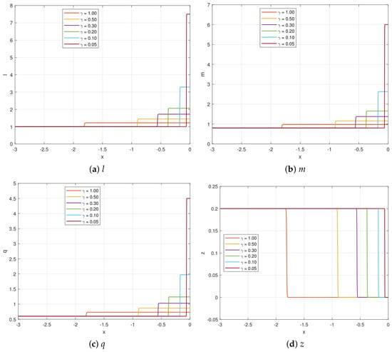
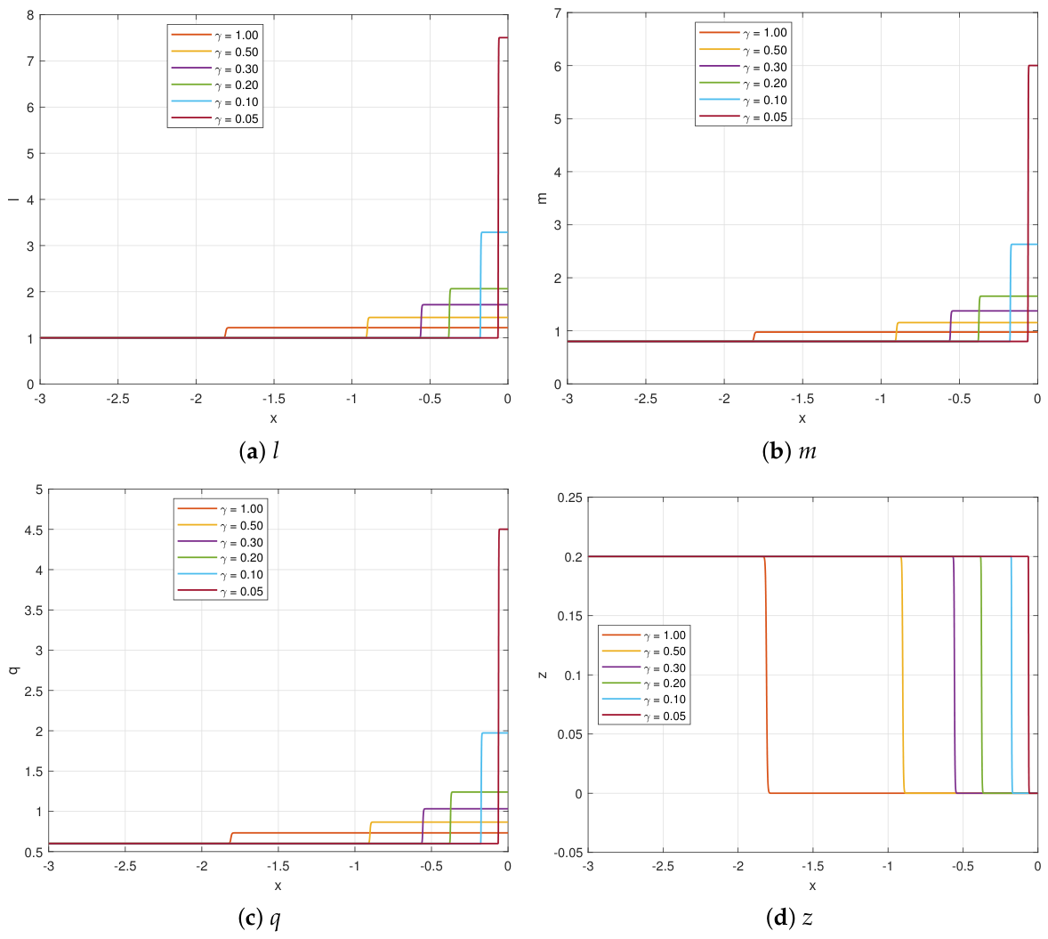
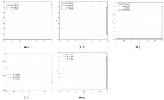
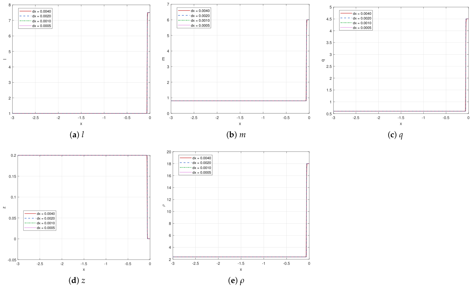
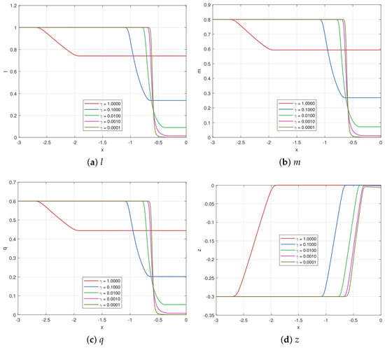
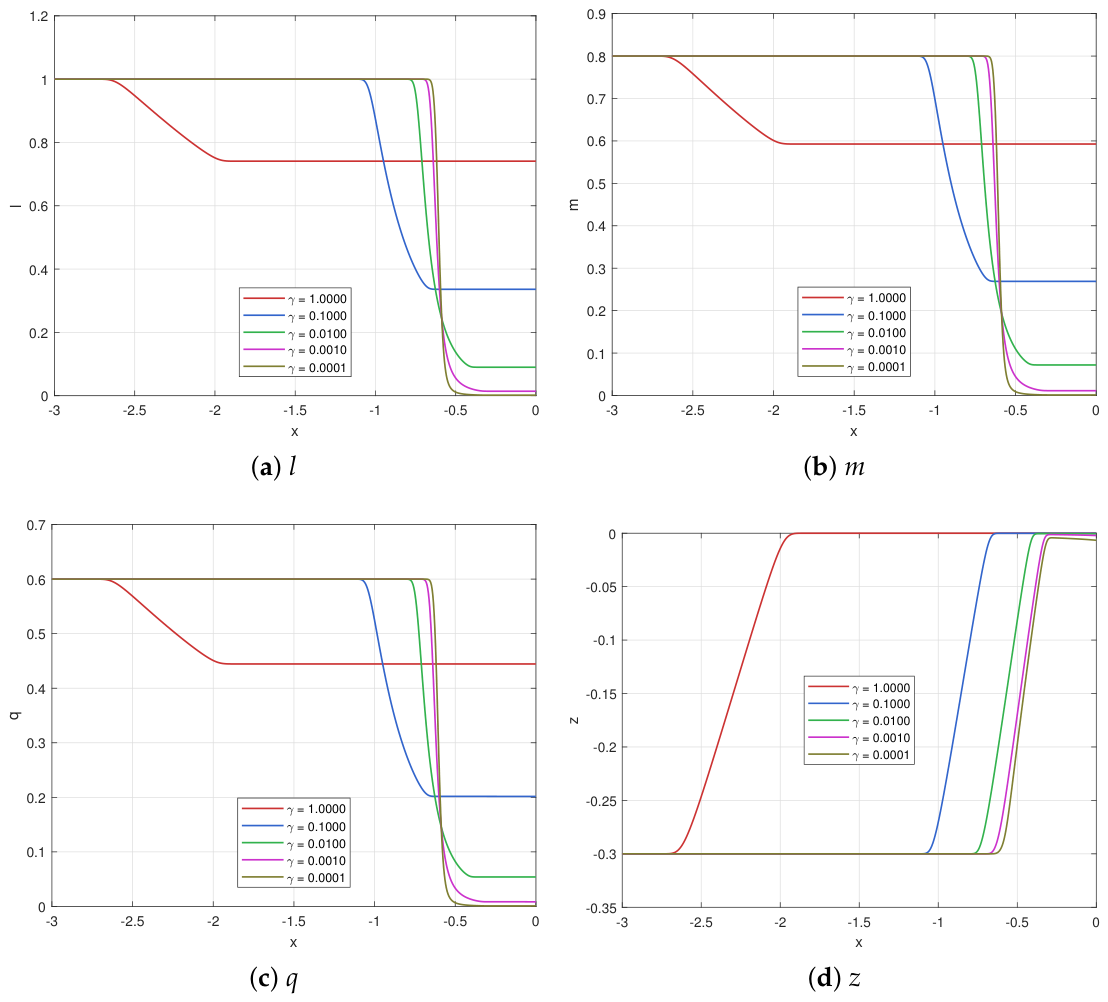
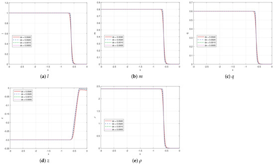
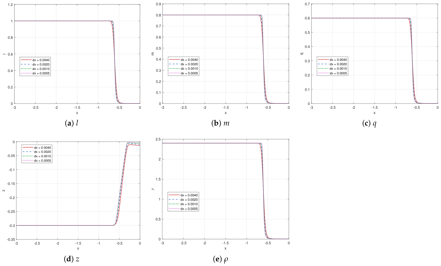
Figure 5 displays the l, m, q, and z profiles at $\mathrm{\Delta }x=0.001$ for decreasing values of $\gamma$. As $\gamma$ is reduced, the three component densities develop increasingly sharp peaks adjacent to the piston, while the relative velocity z approaches zero in an increasingly narrow post-shock region. Figure 6 presents the mesh-refinement results for $\gamma =0.05$. The four tested meshes yield closely agreeing macroscopic profiles, indicating weak mesh sensitivity over the investigated grid range.

Figure 5. HLL solutions of the blockage case for different $\gamma$ values ($\mathrm{\Delta }x=0.001$).

Figure 6. Grid refinement for the blockage case at $\gamma =0.05$.

5.3.2. Quantitative Diagnostics and Approach Toward the Delta-Shock Limit

Table 3 records the numerically measured shock front $x_s$ and the integral weights on the mesh $\mathrm{\Delta }x=0.001$. The shock position is identified as the grid point where $|{\partial }_{x}z|$ attains its maximum. Over the tested finite values of $\gamma$, two asymptotic trends are evident:

Table 3. Quantitative diagnostics for the blockage case at $t=2$ ($\mathrm{\Delta }x=0.001$).

$\mathit{\gamma }$	Scheme	${\mathit{x}}_{\mathit{s}}$	$\int \mathit{l}$	$\int \mathit{m}$	$\int \mathit{q}$	$\int \mathit{\rho }$
$1.00$	HLL	$-1.8105$	$2.2107$	$1.7685$	$1.3264$	$5.3056$
$0.50$	HLL	$-0.9025$	$1.3027$	$1.0422$	$0.7816$	$3.1265$
$0.30$	HLL	$-0.5575$	$0.9577$	$0.7662$	$0.5746$	$2.2986$
$0.20$	HLL	$-0.3765$	$0.7769$	$0.6215$	$0.4661$	$1.8645$
$0.10$	HLL	$-0.1765$	$0.5775$	$0.4620$	$0.3465$	$1.3861$
$0.05$	HLL	$-0.0625$	$0.4650$	$0.3720$	$0.2790$	$1.1159$
Theory ($\gamma \to 0^{+}$)	—	0	$0.4000$	$0.3200$	$0.2400$	$0.9600$

1.

The shock front $x_s$ moves toward the piston from $-1.8105$ at $\gamma =1$ to $-0.0625$ at $\gamma =0.05$, approaching the theoretical limiting position $x_s=0$.

2.

The integral weights move toward the theoretical delta-shock values. For example, $\int \rho dx$ decreases from $5.3056$ to $1.1159$, while the analytical limiting value is $0.96$.

These finite-$\gamma$ results are consistent with the delta-shock asymptotics established analytically in Section 4. Table 4 further examines the mesh sensitivity of these diagnostics at $\gamma =0.05$: the shock position and all integral quantities vary by less than $6\%$ between $\mathrm{\Delta }x=0.004$ and $\mathrm{\Delta }x=0.0005$.

Table 4. Mesh sensitivity of the diagnostics for the blockage case at $\gamma =0.05$.

$\mathrm{\Delta }\mathit{x}$	${\mathit{x}}_{\mathit{s}}$	$\int \mathit{l}$	$\int \mathit{m}$	$\int \mathit{q}$	$\int \mathit{\rho }$
$0.0040$	$-0.0660$	$0.4763$	$0.3810$	$0.2858$	$1.1430$
$0.0020$	$-0.0650$	$0.4703$	$0.3763$	$0.2822$	$1.1288$
$0.0010$	$-0.0625$	$0.4650$	$0.3720$	$0.2790$	$1.1159$
$0.0005$	$-0.0623$	$0.4636$	$0.3709$	$0.2782$	$1.1126$
Theory	0	$0.4000$	$0.3200$	$0.2400$	$0.9600$

5.3.3. Conservation Check

Global mass conservation on the standard mesh $\mathrm{\Delta }x=0.001$ is examined in Table 5. The relative mass error remains below ${10}^{-3}$ for all $\gamma$ values, with the largest error $6.40\times {10}^{-4}$ occurring at $\gamma =0.05$. The theoretical final mass is $M_{\mathrm{theory}}=M_0+{\rho }_0{z}_0{T}_{\mathrm{final}}=7.2+0.96=8.16$, which accounts for the net mass influx across the left boundary ($z_0=0.2$) with the right boundary being impermeable ($z=0$).

Table 5. Conservation check for the blockage case on the standard mesh $\mathrm{\Delta }x=0.001$ ($M_{\mathrm{theory}}=8.16$).

$\mathit{\gamma }$	$\mathrm{\Delta }\mathit{x}$	${\mathit{M}}_{\mathbf{total}}$	$|\mathit{M}-{\mathit{M}}_{\mathbf{theory}}|$	Relative Error
$1.00$	$0.0010$	$8.1601$	$0.0001$	$1.23\times {10}^{-5}$
$0.50$	$0.0010$	$8.1602$	$0.0002$	$2.81\times {10}^{-5}$
$0.30$	$0.0010$	$8.1604$	$0.0004$	$4.99\times {10}^{-5}$
$0.20$	$0.0010$	$8.1606$	$0.0006$	$7.94\times {10}^{-5}$
$0.10$	$0.0010$	$8.1616$	$0.0016$	$1.92\times {10}^{-4}$
$0.05$	$0.0010$	$8.1652$	$0.0052$	$6.40\times {10}^{-4}$

5.4. Asymptotic Behavior When $0<u_0<s_0$ (Rarefaction Case)

The initial data are

$$(l_0,m_0,q_0,u_0)=(1.0,0.8,0.6,0.5),s_0=0.8,$$

yielding the initial relative velocity $z_0=u_0-s_0=-0.3$. The constant-pressure limit predicts a rarefaction head at $x_{\mathrm{head}}=-(s_0-u_0)t=-0.6$, a vacuum region of width $0.6$, and zero minimum density. We select $\gamma =1.0,0.1,0.01,0.001,0.0001$, with the extreme value $\gamma =0.0001$.

5.4.1. Flow Profiles and Grid Refinement

Figure 7 presents the l, m, q, z profiles. As $\gamma$ decreases, the three component densities drop, a vacuum region develops and expands toward the theoretical vacuum interval, and the relative velocity changes from $-0.3$ toward 0 across an increasingly thin transition layer. The mesh-refinement results at $\gamma =0.0001$ shown in Figure 8 indicate that the identified vacuum boundary and the rarefaction transition are similarly resolved on the four tested meshes.

Figure 7. HLL solutions of the rarefaction case for different $\gamma$ values ($\mathrm{\Delta }x=0.001$).

Figure 8. Grid refinement for the rarefaction case at $\gamma =0.0001$.

5.4.2. Quantitative Diagnostics: Vacuum Formation and Asymptotic Trends

Table 6 shows the rarefaction-head position, minimum density, vacuum-width diagnostic, and total mass. The rarefaction-front position $x_{\mathrm{head}}$ is identified numerically as the location of the maximum velocity gradient, $x_{\mathrm{head}}=x\left(\arg \max \right|{\partial }_{x}z\left|\right)$. Since the velocity gradient is approximately uniform across the rarefaction fan, this identification serves as a numerical diagnostic whose limiting position agrees with the theoretical head location $-(s_0-u_0)t$. In the diagnostics below, a cell is labeled as vacuum if $\rho <0.1{\rho }_0$; this is a numerical vacuum criterion on the mesh, not the exact state $\rho =0$. The vacuum region is defined as the set of such grid cells. The minimum density ${\rho }_{\min }$ is the smallest cell-averaged value on the mesh.

Table 6. Quantitative diagnostics for the rarefaction case at $t=2$ ($\mathrm{\Delta }x=0.001$).

$\mathit{\gamma }$	Regime	Scheme	${\mathit{x}}_{\mathbf{head}}$	${\mathit{\rho }}_{\min }$	Vacuum Width	${\mathit{M}}_{\mathbf{total}}$
$1.0000$	No vacuum	HLL	$-2.2845$	$1.7779$	$0.0000$	$5.7603$
$0.1000$	No vacuum	HLL	$-0.8355$	$0.8067$	$0.0000$	$5.7606$
$0.0100$	Vacuum	HLL	$-0.5515$	$0.2159$	$0.4360$	$5.7607$
$0.0010$	Vacuum	HLL	$-0.4995$	$0.0339$	$0.5410$	$5.7603$
$0.0001$	Vacuum	HLL	$-0.5195$	$0.0039$	$0.5680$	$5.7601$
Theory ($\gamma \to 0^{+}$)	—	—	$-0.6000$	0	$0.6000$	$5.7600$

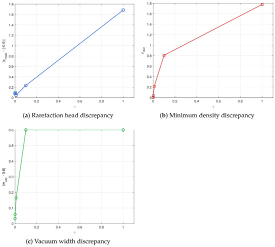
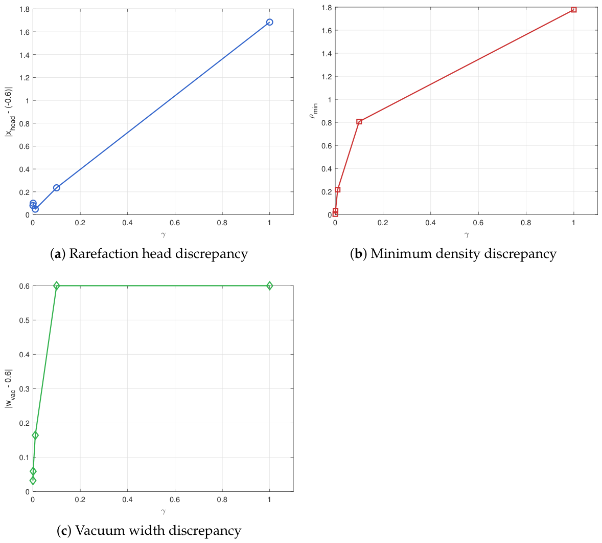
Over the tested values of $\gamma$, the following trends are observed: the identified rarefaction-head position changes from $-2.2845$ at $\gamma =1$ to $-0.5195$ at $\gamma =0.0001$, moving toward the theoretical limiting value $-0.6$; the minimum density decreases from $1.7779$ to $0.0039$; and the vacuum width increases from $0.4360$ to $0.5680$ for the cases in which such a region is detected, while the theoretical vacuum width is $0.6$.

Because the measured width depends on the diagnostic threshold, Table 7 reports the corresponding values for $\rho <0.1{\rho }_0$, $\rho <0.05{\rho }_0$, and $\rho <0.01{\rho }_0$. For $\gamma =0.0001$, the resulting widths are $0.5680$, $0.5520$, and $0.4930$, respectively. For each fixed threshold, the measured width shows an overall tendency toward the theoretical vacuum width as $\gamma$ is reduced. Table 8 indicates that these diagnostics are only weakly sensitive to the mesh at $\gamma =0.0001$: the measured width varies by less than $5\%$ across the meshes. These results indicate that the observed expansion of the numerically resolved vacuum region is robust with respect to the threshold choice over the tested range.

Table 7. Sensitivity of the identified vacuum width to the density threshold ($\mathrm{\Delta }x=0.001$). Theory: $0.6$.

$\mathit{\gamma }$	Regime	${\mathit{w}}_{\mathbf{vac}}(\mathit{\rho }<0.1{\mathit{\rho }}_0)$	${\mathit{w}}_{\mathbf{vac}}(\mathit{\rho }<0.05{\mathit{\rho }}_0)$	${\mathit{w}}_{\mathbf{vac}}(\mathit{\rho }<0.01{\mathit{\rho }}_0)$
$1.0000$	No vacuum	$0.0000$	$0.0000$	$0.0000$
$0.1000$	No vacuum	$0.0000$	$0.0000$	$0.0000$
$0.0100$	Vacuum	$0.4360$	$0.0000$	$0.0000$
$0.0010$	Vacuum	$0.5410$	$0.4910$	$0.0000$
$0.0001$	Vacuum	$0.5680$	$0.5520$	$0.4930$

Table 8. Mesh sensitivity of the diagnostics for the rarefaction case at $\gamma =0.0001$.

$\mathrm{\Delta }\mathit{x}$	${\mathit{x}}_{\mathbf{head}}$	${\mathit{\rho }}_{\min }$	Vacuum Width	${\mathit{M}}_{\mathbf{total}}$
$0.0040$	$-0.4540$	$0.0037$	$0.5480$	$5.7601$
$0.0020$	$-0.4930$	$0.0038$	$0.5600$	$5.7601$
$0.0010$	$-0.5195$	$0.0039$	$0.5680$	$5.7601$
$0.0005$	$-0.5398$	$0.0040$	$0.5740$	$5.7601$
Theory	$-0.6000$	0	$0.6000$	$5.7600$

Mass conservation is again excellent: the relative error is below $3\times {10}^{-4}$ on all grids (Table 9). The theoretical final mass is $M_{\mathrm{theory}}=M_0+{\rho }_0{z}_0{T}_{\mathrm{final}}=7.2-1.44=5.76$, reflecting the net mass efflux across the left boundary ($z_0=-0.3$).

Table 9. Conservation check for the rarefaction case ($M_{\mathrm{theory}}=5.76$).

$\mathit{\gamma }$	$\mathrm{\Delta }\mathit{x}$	${\mathit{M}}_{\mathbf{total}}$	$|\mathit{M}-{\mathit{M}}_{\mathbf{theory}}|$	Relative Error
$1.0000$	$0.0040$	$5.7607$	$0.0007$	$1.23\times {10}^{-4}$
	$0.0020$	$5.7605$	$0.0005$	$7.85\times {10}^{-5}$
	$0.0010$	$5.7603$	$0.0003$	$4.86\times {10}^{-5}$
	$0.0005$	$5.7602$	$0.0002$	$2.93\times {10}^{-5}$
$0.0001$	$0.0040$	$5.7601$	$0.0001$	$1.12\times {10}^{-5}$
	$0.0020$	$5.7601$	$0.0001$	$1.34\times {10}^{-5}$
	$0.0010$	$5.7601$	$0.0001$	$1.21\times {10}^{-5}$
	$0.0005$	$5.7601$	$0.0001$	$9.58\times {10}^{-6}$

Table 10 reports the $L^1$ and $L^2$ profile discrepancies of $\rho$ and $\rho z$ relative to the theoretical vacuum-limit profile. The $L^1$ discrepancy of $\rho z$ decreases from $1.24$ at $\gamma =1$ to $1.48\times {10}^{-2}$ at $\gamma =0.0001$, showing a systematic reduction over the tested values of $\gamma$. This trend is consistent with the constant-pressure rarefaction/vacuum limit established analytically in Section 4.

Table 10. Profile discrepancies relative to the vacuum limit for the rarefaction case ($\mathrm{\Delta }x=0.001$). Limit: $\rho =2.4$ for $x<-0.6$, 0 for $x>-0.6$; $\rho z=-0.72$ for $x<-0.6$, 0 for $x>-0.6$.

$\mathit{\gamma }$	${\mathit{L}}_1\left(\mathit{\rho }\right)$	${\mathit{L}}_2\left(\mathit{\rho }\right)$	${\mathit{L}}_1\left(\mathit{\rho }\mathit{z}\right)$	${\mathit{L}}_2\left(\mathit{\rho }\mathit{z}\right)$
$1.0000$	$2.13\times {10}^0$	$1.59\times {10}^0$	$1.24\times {10}^0$	$9.17\times {10}^{-1}$
$0.1000$	$9.68\times {10}^{-1}$	$1.01\times {10}^0$	$2.26\times {10}^{-1}$	$3.66\times {10}^{-1}$
$0.0100$	$3.17\times {10}^{-1}$	$5.01\times {10}^{-1}$	$6.29\times {10}^{-2}$	$1.59\times {10}^{-1}$
$0.0010$	$1.12\times {10}^{-1}$	$2.75\times {10}^{-1}$	$2.67\times {10}^{-2}$	$8.32\times {10}^{-2}$
$0.0001$	$5.27\times {10}^{-2}$	$1.85\times {10}^{-1}$	$1.48\times {10}^{-2}$	$5.53\times {10}^{-2}$

Figure 9 summarizes the dependence of the three diagnostic discrepancies on the tested values of $\gamma$. The reported discrepancies generally decrease as $\gamma$ is reduced.

Figure 9. Diagnostic discrepancies vs. $\gamma$ for the rarefaction case ($\mathrm{\Delta }x=0.001$).

5.5. Summary

Numerical experiments are performed for finite values of $\gamma$ using the HLL scheme together with $\gamma$-dependent analytical boundary states. Their purpose is to examine whether the observed numerical trends are consistent with the asymptotic results proved in Section 4.

For $s_0<u_0$, as the tested value of $\gamma$ is reduced, the shock front moves toward the piston surface and the integral masses in the post-shock region move toward the corresponding delta-shock weights. On the standard mesh $\mathrm{\Delta }x=0.001$, the relative global mass error remains below ${10}^{-3}$ for all tested values of $\gamma$. These results provide quantitative numerical evidence consistent with the analytically derived delta-shock limit.

For $u_0<s_0$, the minimum density decreases to $O\left({10}^{-3}\right)$ and the numerically identified vacuum region reaches a width of $0.568$ at $\gamma =0.0001$, compared with the theoretical vacuum width $0.6$. The rarefaction-head position, vacuum width, and profile discrepancies of the conservative momentum density $\rho z$ all show an overall tendency toward their corresponding theoretical limiting values as $\gamma$ is reduced. Similar tendencies are obtained for several density thresholds.

Thus, over the tested parameter and mesh ranges, the HLL computations provide quantitative consistency checks for the asymptotic predictions established analytically in Section 4.

6. Conclusions

This paper investigates piston problems for two idealized one-dimensional common-velocity three-component models: the compressible model with $P={\rho }^{\gamma }$($0<\gamma \le 1$) and the constant-pressure model with $P=1$. The models are mathematical prototypes in which all three components share a common velocity and more complex physical effects, such as interphase slip, interfacial momentum exchange, viscosity, and wall friction, are neglected.

According to the relative magnitude of the piston velocity $s_0$ and the initial fluid velocity $u_0$, two basic flow regimes are obtained. For $s_0<u_0$, the compressible model admits an admissible shock solution (7), whereas the constant-pressure model admits a measure-valued delta-shock solution (9) with mass concentration on the piston trajectory. For $u_0<s_0$, the compressible model admits a rarefaction-wave solution (8), while the constant-pressure model admits a vacuum solution (10).

We rigorously establish the asymptotic relation between the two models as $\gamma \to 0^{+}$. More precisely, for each fixed $t>0$, the conservative variables $(l,m,q,\rho u)$ of the solutions to the piston problem for the compressible model converge in the sense of distributions to the corresponding conservative variables of the solutions to the piston problem for the constant-pressure model. In the rarefaction-to-vacuum regime, the convergence statement is formulated only for the conservative variables, because the primitive velocity is not uniquely determined when the total density vanishes.

The HLL computations presented in Section 5 are carried out for finite values of $\gamma$. Over the tested values of $\gamma$, the computed shock locations, accumulated component masses, minimum densities, and vacuum widths move toward their analytically predicted limiting values as $\gamma$ is reduced, providing quantitative numerical evidence consistent with the analytical asymptotic results.

The resulting framework provides a basis for future investigations of more general multicomponent hyperbolic systems and piston problems that incorporate additional physical mechanisms and more complex constitutive laws.

References

- Daude, F.; Galon, P.; Potapov, S.; Beccantini, A.; Mianné, G. A hyperbolic conservative one-velocity one-pressure barotropic three-component model for fast-transient fluid-structure interaction problems. Appl. Math. Comput. 2023, 447, 127919. [Google Scholar] [CrossRef] [Scilit]
- Saurel, R.; Abgrall, R. A multiphase Godunov method for compressible multifluid and multiphase flows. J. Comput. Phys. 1999, 150, 425–467. [Google Scholar] [CrossRef] [Scilit]
- Andrianov, N.; Warnecke, G. The Riemann problem for the Baer-Nunziato two-phase flow model. J. Comput. Phys. 2004, 195, 434–464. [Google Scholar] [CrossRef] [Scilit]
- Johansen, T.E.; Liu, X. Solution of Riemann problems for hyperbolic systems of conservation laws modeling two-phase flow in general stream tube geometries. J. Eng. Math. 2017, 105, 137–155. [Google Scholar] [CrossRef] [Scilit]
- Wei, Z.J.; Sun, M.N. The Riemann problem for a simplified two-phase flow model with the Chaplygin pressure law under the external force. Int. J. Non-Linear Mech. 2022, 144, 104082. [Google Scholar] [CrossRef] [Scilit]
- Jiang, Y.H.; Shen, C. Concentration and cavitation phenomena of Riemann solutions for the isothermal three-component model. Phys. Fluids 2024, 36, 126123. [Google Scholar] [CrossRef] [Scilit]
- Jiang, Y.H.; Shen, C. The adiabatic exponential limits of Riemann solutions in the isentropic three-component model. Math. Comput. Simul. 2026, 241, 48–70. [Google Scholar] [CrossRef] [Scilit]
- Wei, Z.J.; Guo, L.H. The Riemann solutions of the Chaplygin Euler equations with discontinuity terms: The disappearance and generation of a delta shock wave. Commun. Nonlinear Sci. Numer. Simul. 2026, 152, 109170. [Google Scholar] [CrossRef] [Scilit]
- Li, S.W. Delta shock wave as limits of vanishing viscosity for zero-pressure gas dynamics with energy conservation law. ZAMM-Z. Angew. Math. Mech. 2022, 102, E202100377. [Google Scholar]
- Zhang, Q.L. Delta waves and vacuum states in the vanishing pressure limit of Riemann solutions to Baer-Nunziato two-phase flow model. Commun. Pure Appl. Anal. 2021, 20, 3235–3258. [Google Scholar] [CrossRef] [Scilit]
- Evje, S. Global weak solutions for a compressible gas-liquid model with well-formation interaction. J. Differ. Equ. 2011, 251, 2352–2386. [Google Scholar] [CrossRef] [Scilit][Green Version]
- Friis, H.A.; Evje, S. Well-posedness of a compressible gas-liquid model with a friction term important for well control operations. SIAM J. Appl. Math. 2011, 71, 2014–2047. [Google Scholar] [CrossRef] [Scilit]
- Hao, C.C.; Li, H.L. Well-posedness for a multidimensional viscous liquid-gas two-phase flow model. SIAM J. Math. Anal. 2012, 44, 1304–1332. [Google Scholar] [CrossRef] [Scilit]
- Shen, C. The transition of Riemann solutions for the drift-flux model with the pressure law for the extended Chaplygin gas. Phys. Fluids 2023, 35, 046105. [Google Scholar] [CrossRef] [Scilit]
- Shen, C.; Sun, M.N. Exact Riemann solutions for the drift-flux equations of two-phase flow under gravity. J. Differ. Equ. 2022, 314, 1–55. [Google Scholar] [CrossRef] [Scilit]
- Courant, R.; Friedrichs, K.O. Supersonic Flow and Shock Waves; Springer: New York, NY, USA, 1948. [Google Scholar]
- Liu, T.P. The free piston problem for gas dynamics. J. Differ. Equ. 1978, 30, 175–191. [Google Scholar] [CrossRef] [Scilit]
- Slemrod, M. Resolution of the spherical piston problem for compressible isentropic gas dynamics via a self-similar viscous limit. Proc. R. Soc. Edinb. Sect. A Math. 1996, 126, 1309–1340. [Google Scholar] [CrossRef] [Scilit]
- Wang, Z.J. Global existence of shock wave solutions for the one-dimensional piston problem. Chin. Ann. Math. Ser. A 2005, 26, 549–560. [Google Scholar]
- Ding, M.; Li, Y.C. Stability and non-relativistic limits of rarefaction wave to the 1-d piston problem for the relativistic Euler equations. Z. Angew. Math. Phys. 2017, 68, 43. [Google Scholar] [CrossRef] [Scilit]
- Qu, A.F.; Yuan, H.R. Measure solutions of one-dimensional piston problem for compressible Euler equations of Chaplygin gas. J. Math. Anal. Appl. 2020, 481, 123486. [Google Scholar] [CrossRef] [Scilit]
- Wang, Z.Q.; Guo, L.H.; Wei, Z.J. Piston problem for the pressureless hydrodynamic traffic flow model. Phys. Fluids 2024, 36, 056118. [Google Scholar] [CrossRef] [Scilit]
- Huang, M.; Wang, Y.; Shao, Z. Piston problem for the generalized Chaplygin Euler equations of compressible fluid flow. Chin. J. Phys. 2024, 89, 810–819. [Google Scholar] [CrossRef] [Scilit]
- Whitham, G.B. Linear and Nonlinear Waves; Wiley-Interscience: New York, NY, USA, 1974. [Google Scholar]
- Chen, H.H.; Sheng, W.C. Piston problem for Euler equations of Van der Waals gas. Chin. Ann. Math. Ser. A 2020, 41, 263–278. [Google Scholar]
- Lefrançois, E.; Boufflet, J.P. An introduction to fluid-structure interaction: Application to the piston problem. SIAM Rev. 2010, 52, 747–767. [Google Scholar] [CrossRef] [Scilit]
- Feireisl, E.; Mácha, V.; Nečasová, Š.; Tucsnak, M. Analysis of the adiabatic piston problem via method of continuum mechanics. Ann. Inst. Henri Poincaré Anal. Non Linéaire 2018, 35, 1377–1408. [Google Scholar] [CrossRef] [Scilit]
- Huang, M.X.; Wang, Y.J.; Shao, Z.Q. Piston problem for the isentropic Euler equations for a modified Chaplygin gas. Phys. Fluids 2023, 35, 016119. [Google Scholar] [CrossRef] [Scilit]
- Noorizadegan, A.; Cavoretto, R.; Young, D.L.; Chen, C.S. Stable weight updating: A key to reliable PDE solutions using deep learning. Eng. Anal. Bound. Elem. 2024, 168, 105933. [Google Scholar] [CrossRef] [Scilit]
- Davis, S.F. Simplified Second-Order Godunov-Type Methods. SIAM J. Sci. Stat. Comput. 1988, 9, 445–473. [Google Scholar] [CrossRef] [Scilit]
Disclaimer/Publisher’s Note: The statements, opinions and data contained in all publications are solely those of the individual author(s) and contributor(s) and not of MDPI and/or the editor(s). MDPI and/or the editor(s) disclaim responsibility for any injury to people or property resulting from any ideas, methods, instructions or products referred to in the content. |
© 2026 by the authors. Licensee MDPI, Basel, Switzerland. This article is an open access article distributed under the terms and conditions of the Creative Commons Attribution (CC BY) license.