


Abstract
Group decision-making sometimes involves evaluating the decision-makers themselves, e.g., selecting the best expert or assigning rewards within a team. In such cases, all participants should be involved, but their influence should reflect their competence or contribution. This article proposes two new opinion aggregation models in which a person’s assessment weight depends on their ranking, preventing low-performing members from exerting the same influence and promoting respected experts. The proposed aggregation methods uphold the principle of distributive justice by ensuring that individual contributions are proportional to the rewards they receive. In addition to formulating new methods for aggregating results, we presented several of their formal properties and indicated practical ways to calculate the results. For one of the methods, which is more challenging to compute, we conducted a Monte Carlo experiment demonstrating the practical feasibility of computing the aggregated weight vector.
Keywords:
group decision-making; aggregation of individual rankings; pairwise comparisons; distributive justice; equity theory; softmax; aggregation operators; Analytic Hierarchy Process MSC:
90B50; 15A24; 47J26; 60J20
1. Introduction
From time to time, we see discussions about which expert is more competent, which of specialist is more professional, which of specialist of merit to the country is more distinguished, etc. The reason for such discussions is most often the need for an award, a diploma of recognition, or a medal in recognition of service to the country or work for an organization. Sometimes, the award is financial and given to everyone who has earned it. In this case, the issue to be resolved is the award’s distribution among all concerned. A specific group of people with expertise in the subject being evaluated selects the best candidate or decides on the award distribution. Having such expertise, however, means that these individuals may be the subject of the evaluation. A similar situation occurs with the distribution of awards for various other team achievements, such as grants, organizational projects, or software projects in IT companies. The solution proposed in this paper is based on the aggregation procedure used in the group decision-making (GDM) process, which is used in the pairwise comparison method. This approach has also resulted in several studies in group decision-making. Traditionally, the Analytic Hierarchy Process (AHP) builds on two opinion aggregation procedures: aggregation of individual judgments (AIJ) and aggregation of individual priorities (AIP) [1,2,3,4]. In the AIJ procedure, experts first combine their pairwise comparison (PC) matrices into a collective judgment matrix and then derive a group priority vector. In contrast, in the AIP procedure, they first compute individual priority vectors and subsequently aggregate them into a collective priority structure. Section 2.2.3 presents the latter approach in greater detail. The literature widely accepts and applies both procedures for aggregating preferences expressed in the form of PC matrices (see Section 2.1); however, Forman and Peniwati [4] recommend AIJ in situations where experts agree in advance on a common assessment framework, as this agreement facilitates coherent judgment aggregation at the group level. Ramanathan and Ganesh [5] advocate aggregating individual priorities (AIP), showing that this procedure satisfies the Pareto principle when decision-makers derive priorities using the eigenvector method (EVM) introduced by Saaty [1]. In contrast, their analysis demonstrates that aggregation of individual judgments (AIJ) may violate the Pareto principle under the same prioritization scheme, highlighting a fundamental theoretical distinction between the two aggregation approaches and informing the choice of aggregation procedure in AHP-based group decision-making contexts. Both methods are equivalent when using the geometric mean method (GMM) or logarithmic least square method (LLSM) (both GMM and LLSM are equivalent for complete and incomplete PC matrices [6]) for the ranking calculation [7]. In addition to the two methods mentioned above, other methods of aggregating preferences have emerged. Blagojević et al. [8] introduce a GED-based aggregation method for AHP group decision-making, employing simulated annealing to heuristically minimize the distance between individual and group judgments. While effective in handling complex preference structures, the approach is computationally demanding and lacks explicit consensus and consistency in modeling. Dong et al. [9] propose a consensus model for AHP group decision=making in which individual preference matrices are iteratively adjusted to minimize a geometric consensual consistency index (GCCI), showing that this process improves group agreement under the row geometric mean method; nevertheless, the approach is developed for static expert settings and fixed consensus parameters, leaving room for later extensions addressing its adaptability and scalability. Altuzarra et al. propose the Bayesian prioritization procedure (BPP), allowing for the aggregation procedure to be extended to preferences (utilities, priorities) among alternatives, which are presented as probability distributions [10]. Escobar and Moreno-Jimenez [11] propose the Aggregation of Individual Preference Structures (AIPS) method for AHP group decision-making, demonstrating that aggregating individual preference structures can better preserve decision-makers’ preference information; nevertheless, the method does not explicitly incorporate consensus control or a means of inconsistency reduction, which is addressed in later studies. Lin et al. [12] propose an aggregation framework for AHP-based group decision-making in which individual pairwise comparison matrices are first transformed into their nearest consistent matrices and then aggregated under an acceptable-consensus constraint. The study demonstrates that incorporating a consensus adjustment improves group agreement while preserving individual consistency properties; however, the proposed approach assumes fixed consensus thresholds and focuses on static group settings, without addressing computational scalability or the dynamic evolution of opinions, which motivates subsequent research on adaptive, computationally efficient, consensus-driven aggregation methods.
Researchers have extended classical aggregation procedures to decision models that represent preferences using interval-valued judgments [13] and fuzzy sets [14], thereby capturing the uncertainty and imprecision inherent in group assessments. Building on this line of research, Mateos et al. [15] introduce a group decision-making (GDM) methodology for settings with incomplete individual beliefs, in which the voting weight of political representatives reflects the electoral support they receive. This approach illustrates how aggregation mechanisms can incorporate contextual information beyond preference judgments; however, it also raises concerns regarding the strategic manipulation of expert influence. Addressing this issue, Kułakowski et al. [16] propose a resilient heuristic aggregation framework that adaptively adjusts expert weights to mitigate manipulation attempts, thereby enhancing the robustness of opinion aggregation in pairwise comparison-based decision models. Zhao et al. [17] focus on individual participation and satisfaction in group decision-making and explicitly incorporate fairness and tolerance into the consensus-formation process. They propose a consensus model that maximizes aggregated utility expressed through an additive Choquet integral, which captures interactions among decision-makers’ preferences rather than treating them as independent. Their results show that the model can balance collective agreement with individual utility and satisfaction; however, the approach relies on eliciting interaction indices and assumes a static preference structure, which may limit its applicability in large-scale or dynamically evolving decision environments, and motivates further research on scalable, adaptive utility-based consensus models.
Decision-making methods are also used in situations where the interested parties (evaluators) evaluate each other. James et al. [18] address the peer assessment problem as a specific instance of group decision-making and focus on improving the reliability of aggregated evaluations. They propose a moderation-oriented framework that identifies potentially unreliable assessors by combining reliability indices with a consensus analysis of peer scores. Their numerical experiments show that this two-angle approach can effectively flag a subset of peer assessments for expert moderation, thereby increasing scoring accuracy while reducing the overall workload of subject experts. However, the proposed methodology targets static assessment settings. It assumes access to sufficient peer-evaluation data, which limits its applicability in highly dynamic environments or in cases with sparse or strategically biased assessments, thereby motivating further research on adaptive and manipulation-resistant moderation mechanisms within GDM frameworks. Luo et al. [19] investigate peer grading in the context of Massive Open Online Courses (MOOCs) by analyzing 1825 peer-reviewed assignments collected from a Coursera course. The authors assess the reliability and validity of peer grading by comparing aggregated peer scores with instructor evaluations and by examining students’ perceptions of the assessment process. Their empirical results show that student graders’ collective judgments closely match instructor scores, and that most participants perceive peer grading as fair and beneficial, supporting the practical usefulness of peer assessment in large-scale learning environments. Nevertheless, the study focuses on a single MOOC setting. It relies on aggregate agreement measures, leaving open questions about individual grader bias, strategic behavior, and the robustness of peer-grading mechanisms across diverse courses and learner populations. Capuano et al. [20] address the problem of peer assessment in MOOCs by using Fuzzy Ordinal Peer Assessment (FOPA), a group decision-making model designed to handle unreliable and incomplete ordinal evaluations provided by students. The two-step FOPA procedure first completes partial rankings by transforming them into fuzzy preference relations and estimating missing values. Then, it aggregates the enriched preferences using ordered weighted averaging (OWA) operators. Experimental results show that FOPA improves both ranking reconstruction and grade estimation when compared with existing ordinal and cardinal peer assessment methods, thereby demonstrating the practical value of fuzzy aggregation in large-scale educational settings. However, the approach requires eliciting fuzzy intensity judgments and entails additional computational overhead, which may limit its scalability and ease of adoption in very large or time-constrained MOOC environments, and motivates further research on simpler yet robust ordinal aggregation mechanisms. Langan et al. [21] examine evaluation and self-evaluation within the student–teacher relationship by analyzing peer, self, and tutor assessments of oral presentations in higher education. The authors investigate how student characteristics, such as gender and academic attainment, influence assessment outcomes and compare the resulting marks across the three evaluation modes. Their findings show that peer assessments align more closely with tutor evaluations than self-assessments, while self-evaluation exhibits systematic biases, notably gender-related underestimation of performance by female students. The study also reveals contextual effects, including grading compression among peers and variability linked to session structure and student conditions, such as fatigue. Although the empirical analysis provides valuable insights into sources of bias in educational assessment, the work focuses on a specific assessment format and institutional setting, limiting the generalizability of the results and motivating further research on bias-aware, context-adaptive aggregation mechanisms for self- and peer evaluations.
In the above-mentioned works, even when differences in experts’ priorities appear, they result either from external intervention (moderation) [18], from automatic rules aimed at achieving decision consensus [9,12], or from assessments of an expert’s quality based on their past performance [22]. To the best of our knowledge, however, no study has addressed a situation in which an expert’s priority (i.e., an assessment of their quality) is determined simultaneously with their participation in the decision-making process. This gap in the literature is precisely what the present work aims to address.
To address this gap, we introduce two alternative opinion aggregation methods for situations in which evaluators and evaluated individuals coincide. Both methods (additive and multiplicative) make the strength of a given expert’s voice (the weight of their opinion) dependent on the evaluation result they have received. Thus, the more respected a given expert is (and, therefore, the more they deserve the award), the greater the weight assigned to their opinions. Conversely, the less respect a person enjoys within the group, the less influence their opinion has on the final result. A defined additive method always admits a solution that is computable via an iterative procedure. In our work, we indicate the convergence speed of iterations. The additive method also always has a solution. However, it is not always possible to calculate it using the iterative procedure. In this case, the use of optimization methods is more important. Formal analysis proves the existence of a global solution and identifies the condition for its uniqueness. In addition, Monte Carlo experiments demonstrate the effectiveness of the calculations in the multiplicative case. The paper also analyzes the properties of both aggregation functions. One of the motivations for undertaking this topic in the paper was the problem of fairness, often colloquially expressed in the statement “equal does not mean fair.” For this reason, in the conclusion of the paper, we discuss the relationship between the proposed aggregation methods and the equity theory. The presented research will help to create more fair models for aggregating the opinions of experts and decision-makers.
The article consists of eight parts. The Introduction (Section 1) and Preliminaries (Section 2) are intended to familiarize the reader with the subject’s literature and recall the necessary concepts and definitions related to the pairwise comparison method and group decision-making. The third section, “Peer Ranking Aggregation,” describes the problem of a group of experts’ self-assessment, introduces the proposed two methods of aggregating the results, additive and multiplicative, and indicates how to calculate the results. This section also contains theorems concerning the existence of a solution and its uniqueness in the multiplicative problem. Section 4 analyzes the properties of the defined methods. The next section indicates the place of the proposed aggregation methods in the decision-making process. The sixth section contains an analysis based on Montecarlo’s experiments, showing, in practice, the possibility of calculating the result in the multiplicative case. The last two sections of the paper discuss the relationship between the proposed aggregation methods and the issue of equity, and summarize the proposed aggregation functions and the obtained results.
2. Preliminaries
2.1. Pairwise Comparisons
Many methods, including AHP, HRE, MACBETH, and BWM, as well as outranking methods like PROMETHEE [6,23], and various hybrid solutions, use pairwise comparisons (PC) as a source of information about decision-makers’ preferences. The approach has been extended to cover different data representations, including intervals [24], fuzzy sets [14], or gray numbers [25]. The best-known method based on pairwise comparisons of alternatives is AHP. This is also the most criticized, although the criticism is often constructive and has led to many improvements and extensions of the original proposal. Among the more critical areas of improvement are the methods for calculating the vector of weights [26], including ranking incomplete matrices [27,28,29], methods for measuring inconsistencies [30,31], and others. One can find an interesting critical analysis of the AHP method in the work of Munier and Hontoria [32].
In the PC method, experts, also known as decision-makers, compare alternatives in pairs. Let be a finite set of alternatives and a set of experts. Each expert compares the alternatives with each other to form a set of comparisons represented in the form of a square matrix where , and q indicates the number of the expert. A single denotes the relative importance of the i-th alternative compared to the j-th alternative according to the expert’s opinion . For the sake of legibility of notation, whenever possible we will omit the expert index q by writing the PC matrix as . The PC matrix is used to synthesize a vector of weights. Let us define the function resulting from this calculation.
Definition 1.
Let A be a set of alternatives. The priority function for A is the mapping assigning a real and positive number to each alternative.
The priority vector for A resulting from takes the following form:
Many methods have been described in the literature to calculate the value of priority vector w. The first one, which is still quite popular, is the eigenvalue method (EVM). Saaty proposed this approach in his seminal paper [1], and it consists of calculating a principal eigenvector and then normalizing it so the sum of entries is one. Another method is based on calculating the geometric means (referred to as the geometric mean method (GMM).) of the matrix rows and taking the result of the i-th row as the priority of the i-th alternative [33]. The result thus obtained is also subject to normalization at the end of the calculation. In addition to the two mentioned methods, several others for calculating the priority vector exist. For example, Srdjevic et al. compare the performance of the six popular priority-deriving methods [34]. Other examples of prioritization methods can be found in [35,36].
The matrices used in the pairwise comparison method have several specific properties. Below, we recall the Frobenius–Perron theorem as it applies to matrices used in opinion aggregation.
Definition 2.
A square matrix A is stochastic if all of its entries are non-negative, and the entries of each column sum to . A matrix is positive if all of its entries are positive numbers [37] (p. 349).
Theorem 1.
Let A be a positive stochastic matrix. Then, A admits a unique normalized steady state vector x, which spans the -eigenspace. Moreover, for any vector with entries summing to some number c, the iterates
approach as t becomes large [37] (p. 351).
Claim 1.
From the above assertion, the following statements are true [37] (p. 351):
- 1.
- The -eigenspace of a positive stochastic matrix is a line.
- 2.
- The -eigenspace contains a vector with positive entries.
- 3.
- All vectors approach the -eigenspace upon repeated multiplication by A.
In pairwise comparison matrix analysis, an important element is the analysis of matrix inconsistency.
Definition 3.
The pairwise comparisons matrix with dimensions is consistent if for every holds .
The basic methods for determining the degree of inconsistency among pairwise comparison matrices are inconsistency indices. Many different inconsistency indicators can be found in the literature [30,31]. The most commonly used and earliest introduced is that defined by Saaty [1], as follows:
where is the spectral radius of a square matrix C with dimensions . For a valid multiplicative pairwise comparison matrix with reciprocity, i.e., for every holds , it is true that . Whereby when C is consistent, i.e., . For the purposes of AHP, Saaty also defined the consistency ratio , understood as the quotient of the inconsistency index of matrix C and the average value of the inconsistency index for a random matrix of pairwise comparisons with the given dimensions and comparison scale. He suggested that matrices for which the value of CR is no greater than (a matrix at least 10 times more consistent than a comparable random matrix) should be treated as sufficiently coherent and the weight vector calculated on this basis is considered credible.
The measurement of inconsistency applies to a single matrix in pairs. In the case of multiple experts and multiple matrices, a different method of determining their concordance is required. One such method is Saaty’s compatibility index [6,38], given as follows:
where ⊙ is a Hadamard product of and . If both matrices are fully compatible with each other, their compatibility index (3) is equal to 1. Other ways of determining and improving the concordance (consensus) of weight vectors from different experts can be found in the literature [39]. These could include, for example, checking the distance of a given expert’s opinion from the average recommendation, combined with the elimination of outliers [16] or calculating the GCCI (Geometric Cardinal Consensus Index) and GOCI (Geometric Ordinal Consensus Index) group incompatibility measures [9], among others.
2.2. Group Decision-Making
2.2.1. Aggregation Procedures
When more than one expert participates in decision-making, their opinions must be aggregated. As with a single PC matrix, the final result should be a vector of weights assigning real numbers to each alternative. The aggregation of expert opinions can be achieved both at the level of individual comparisons and at the level of individual weight vectors. An example of the first approach is the AIJ (aggregating of individual judgments) [4] procedure, according to which each comparison of the i-th and j-th alternatives by each of k experts is averaged, and then a vector of weights is calculated for the matrix composed of the averaged values. In addition to AIJ, several optimization methods directly use expert comparison results. The previously mentioned model, based on minimization of group Euclidean distance (GED) values [8], is an example. A different approach is the AIP procedure, in which priority vectors for individual experts are calculated first, and only then are the results aggregated. Compared to AIJ, the AIP approach has several significant advantages. One undoubted advantage of the AIP approach is that both geometric and arithmetic averages can be used to aggregate preferences [4]. Moreover, the second method does not impose the need for a group of experts to act as a unit, leaving them more freedom to make individual judgments [4]. It can also be easily implemented in the case of incomplete data from different experts. In such cases, it is sufficient to use appropriate prioritization methods for incomplete PC matrices [27,29] to calculate individual weight vectors. The weight vectors obtained in this way may then be subjected to aggregation. In addition, AIP satisfies the Pareto principle with an arithmetic or a geometric mean.
Aggregation procedures allow each expert’s opinion to be assigned a different strength (priorities). Thus, experts considered less competent can have less influence on the final opinion, while more recognized experts can significantly impact the final outcome. In the following two sections, we will look at two variants of the AIP method that allow for different priorities to be assigned to individual experts.
2.2.2. Additive Aggregation of Individual Priorities
Let the vector of weights calculated from the pairwise comparison matrix provided by the q-th expert be denoted as follows:
Then, let W be a matrix of weight vectors so that
i.e.,
and let p be the vector of priorities for individual experts, i.e.,
so that . Then,
denotes the AIP procedure using a weighted arithmetic mean. To simplify the notation, we will omit the vector p when the priorities of the experts are equal, i.e.,
2.2.3. Multiplicative Aggregation of Individual Priorities
Let the priority vector provided by the q-th expert be (4), the matrix of priority vectors be W (5), and the vector of expert priorities be p (6), so that . Then,
denotes the AIP procedure using a weighted geometric mean. As before, we will drop the vector p in a situation of equal priorities, i.e.,
3. Peer Ranking Aggregation
3.1. Problem Description
Sometimes, the expert team members have to perform a peer self-assessment. This may be related, for example, to selecting the best expert, distributing a reward for achieving an intended goal, or creating a ranking of experts for any other purpose. The evaluation criterion can be professionalism, commitment to the team, or simply appreciation of others. In such a situation, team members, on the one hand, become the subjects of evaluation themselves; on the other hand, they have the knowledge and appropriate competence to participate as experts (decision-makers) in the review. However, while their participation as experts in the decision-making process seems necessary, the weight of their opinions should be tied to the assessment they received. For example, an expert who is recognized by their colleagues should have a greater influence on the team’s work outcomes than those rated lower. We may encounter such a situation when the team is small, and there is no possibility of selecting or naming an impartial person to evaluate team members. Such a team may, for example, be a small group of collaborating scientists preparing a joint publication, a team of peer programmers developing a joint application, an autonomous task force in an organization that needs to distribute bonuses, etc. To handle such situations, we propose two methods of aggregating expert evaluations. In our proposal, the weight of a given expert’s voice depends on the ranking score they receive.
3.2. Assessment-Driven Aggregation Model (ADAM)
The above considerations led us to propose a modified peer-review model based on pairwise comparisons of alternatives. In the solution presented, group members have a dual role. They are simultaneously the object of comparison, i.e., the alternatives in the PC method, and the experts providing their judgments, i.e., . Each of the experts, i.e., team members, provides comparisons in the form of a PC matrix , where , in which they assess the relative level of recognition of the other members of the group. Based on the collected ratings ,…,, vectors of weights are created for individual experts. The calculated vectors are then subjected to aggregation, resulting in the formation of a final priority vector:
reflecting the share of each person evaluated for the award. However, in line with the observation that people who are more respected are often more competent judges of others, the priorities given to expert opinions during aggregation may differ to reflect this regularity. Therefore, let be an expert priority function such that, for two experts and , if their final evaluation share meets , then their priorities during the aggregation process also meet . This regularity follows from the observation that individuals held in higher esteem by their peers have a correspondingly stronger claim to influence the distribution of the reward. Accordingly, we adopt the identity mapping , which assigns decision-making power is directly in proportion to the level of recognition expressed in the assessment process. This choice preserves the proportional relationship between recognition and influence without introducing additional normative assumptions or distortions, ensures that aggregation remains strictly assessment-driven, and offers a transparent and easily interpretable mechanism. For these reasons, the identity function constitutes not only the simplest but also, in the considered context, the most equitable specification of p. Below, following [4], we propose two assessment-driven aggregation methods to support the proposed ADAM model: multiplicative and additive.
3.3. Additive Assessment-Driven Aggregation Method (AADAM)
When proceeding to aggregate the results, we assume that each team member provided a PC matrix , based on which the ranking vector was calculated. These vectors form a matrix W (see (5)). Denoting the vector of experts’ priorities as we obtain an extra condition that the final solution must satisfy:
where for and for any it holds that . The above condition (9) states that the ranking values of the individual alternatives/experts (i.e., the right side of the equation) are equal to the priorities (after normalization) with which the opinions of the individual experts were considered (the left side of the equation). The Equation (9) is
Since W is a stochastic matrix and irreducible and aperiodic, i.e., , and for ; thus, due to the Perron–Frobenus theorem (see Theorem 1) there is a unique and positive eigenvector with the eigenvalue 1 whose entries add up to one. Thus, (10) takes the form
Moreover, the vector p can be calculated iteratively as the limit of the iteration procedure where entries of the initial vector have to sum up to 1. Using properties of W, we can easily estimate the convergence speed of an iterative method.
Property 1.
Since , the matrix is primitive, so its principal eigenvalue is and all other eigenvalues satisfy . Let be the second largest eigenvalue (SLEM). Then, [40] (p. 331). Hence, the number of iterations needed to achieve accuracy ε (e.g., ) is in the order of , and for the number is .
It is worth noting that eigenvector calculation algorithms W, as well as global optimization methods, can also be used to calculate the solution. For example, condition (9) induces the following optimization problem:
whose solution is the sought-after vector p (10).
Regardless of the calculation method adopted, we will denote the aggregation result using this model as , where W is a matrix in which the columns are vectors of weights derived from individual experts.
3.4. Multiplicative Assessment-Driven Aggregation Method (MADAM)
In the case of the geometric mean, the condition (9) takes the following form:
where for .
The equivalent non-linear optimization problem is as follows:
The accepted constraints correspond to the conditions of the MAIP problem, i.e., the value of priorities for each expert is positive and their sum is 1. The above (13) can be solved using constrained global optimization methods. One can also attempt to find the final vector of weights using a direct iterative algorithm (DIA); however, is should be noted that it may not always converge. The iterative algorithm works according to the following scheme.
If the Algorithm 1 returns the correct value of the vector of weights, this result can be taken as the correct solution. If the calculated result is too inaccurate, we can increase the number of iterations and try to run the algorithm again. However, if the calculation does not converge despite increasing parameters and , it is necessary to use dedicated software with optimization algorithms. Regardless of the calculation method adopted, we denote the aggregation result using this model as , where W is a matrix in which the columns are vectors of weights derived from individual experts.
| Algorithm 1 Direct Iterative Algorithm (DIA) |
|
The computational complexity of the DIA algorithm, assuming that the standard 64-bit representation of a real number, is the maximum of the computational complexity of , and vector normalization multiplied by the maximum number of iterations . Since , have a complexity of and normalization has a linear complexity, the final execution time of the DIA algorithm is = ( is a constant).
3.5. The Existence of a Solution in the Multiplicative Approach
In both approaches, i.e., additive AADAM and multiplicative MADAM, the solution exists. However, while in AADAM its existence was almost immediate and resulted from a well-known property of the stochastic matrix, in the multiplicative case this fact requires separate justification. Let us, therefore, show that the MADAM optimization problem (13) always has a solution, i.e., function g always reaches the global minimum. To present this statement in the form of a theorem, for convenience, let us shorten the notation by assuming , , , and .
Theorem 2.
For such that where and for there is always a global minimizer , such that .
Proof.
Note that the condition is equivalent to , where . Thus, . It is the case that , where is a closed unit sphere in [41] (p. 11). Let us define
and . Since for every , then for every , holds. It is also true that the function is a continuous function on . Let have the following mapping:
Function F is continuous and well-defined. The denominator is positive because and, for the same reason, all its components are strictly positive. Since is a closed unit sphere (compact and convex), and F is continuous, then according to Brouwer’s theorem [41] (p. 220) there exists such that .
Let us adopt the following as the minimum required:
where, of course, it holds that
Unfortunately, the above statement does not guarantee that the minimum found is unique. However, we can attempt to formulate a sufficient condition for the existence of a unique solution to problem (13). To achieve this end, let us define a measure of agreement between the expert opinions contained in W (5).
Definition 4.
For a given matrix , where the rows are weight vectors derived from experts, let us take the matrix of logarithms . Let be given as
We will refer to as the index of disagreement among the experts’ opinions presented in matrix W, where
In deed, if the i-th and k-th rows in matrix W are identical, then . If they are similar, i.e., , then . The introduction of the disagreement index allows us to set an easily numerically verifiable condition for the existence of a unique global solution using the MADAM method.
Theorem 3.
The solution to problem (13) is unique if the preferences of the experts expressed in the matrix W are sufficiently similar, i.e., if .
Proof.
Using the notation from Theorem 2, let us observe that Hence,
Therefore, for the matrix , we have
Thus, taking the definition (15), we can see that , where is the softmax function, given as
Let us consider , where , i.e., ; we obtain
Thus,
Let us define the variance of the vector elements as . Thus, due to (20), it holds that
From Lemma 1 (proven below), it holds that . Bearing in mind that , we obtain the following:
From Banach’s fixed point principle [41,42] we know that there is exactly one , such that if F is a contraction, i.e., there exists a Lipszyc constant , such that . Therefore, for F to be a contraction, the following is necessary:
which is true when
□
Additionally, let us prove the property of the softmax function that we used in the above theorem.
Lemma 1.
For the softmax function , defined as , and the variance of variables for vector r, given as , it holds that
Proof.
Let denote the Jacobian matrix of the softmax function. We know [43] that , where . Furthermore, for , the following inequality holds:
Hence, due to Minkowski’s integral inequality
For any , denote (weighted average x as ). Since and , then
Therefore,
For any numbers and any weight distribution , the following holds:
where . Hence, in particular, it follows that
□
Theorem 3 defines a simple, numerically verifiable, sufficient condition for a global solution to be a unique solution of an optimization problem (13). However, this is not a necessary condition. This means that even if the conditions of this theorem are not met, the global minimum of the function g may still be unique.
3.6. Illustrative Example
The opinion aggregation models proposed above can be applied in many cases. To illustrate how and in what context the above models can be used, let us consider the following example.
Example 1.
Four scientists—John, Samantha, Michael, and Frank—of equal seniority and professional experience worked on a joint project that resulted in a scientific article. John proposed the research idea and coordinated the team’s activities. However, during the project, Samantha’s ideas substantially reshaped the research plan, and she ultimately made the largest contribution. She also collaborated most intensively with the other team members. Michael wrote the software and ran the experiments. After completing the initial programming tasks, he focused mainly on testing various data sets and collaborated only occasionally with other team members. Frank collected and prepared the experimental data but did not participate in most team meetings. The team published the results in a respected journal. The university awarded the team a financial prize and left its distribution to the project participants. John, Samantha, Michael, and Frank agreed that each researcher’s share of the award should reflect their contribution and involvement in the project. At the same time, they noted that the ability to evaluate contributions accurately increases with the level of involvement. As a result, they proposed that each participant evaluate all team members using pairwise comparisons and aggregate the resulting opinions with the AADAM method, which appropriately differentiates the priorities of individual experts.
John observed that Samantha invested substantially more effort and commitment than the others. However, he believed that the original idea and initiative carried equal importance. Therefore, he rated Samantha’s contribution as equal to his own. He rated Michel’s and Frank’s contributions as two and three times smaller than his own, respectively. Consequently, his pairwise comparison matrix takes the following form:
Samantha believes that the actual amount of work performed should guide the distribution of the award. Moreover, she considers her ideas to be at least as relevant as, and possibly more relevant than, John’s. Accordingly, she rated her contribution slightly higher than John’s. She rated Michael’s and Frank’s contributions as three and four times lower than her own, respectively. Consequently, her set of judgments, represented by the matrix looks as follows:
Michael recognizes that his contribution to the project was smaller than that of the others. However, he communicated more frequently with Samantha than with the other team members. Consequently, he perceives her contribution as more important than John’s. In his view, the amount of work and time Frank devoted exceeded half of his own contribution. Accordingly, his judgments, represented by the matrix are as follows:
Frank realistically assesses his role in the project. He considers his participation in the project to be non-critical. He assigns similar importance to the contributions of the two key researchers, John and Samantha. Accordingly, he does not differentiate between their levels of participation. He views his own involvement in the project as ancillary. He holds a similar view of Michael’s role. Therefore, he evaluates Michael’s contribution as comparable to his own. As a result, his set of evaluations, given as matrix , is as follows:
After calculating the priority vectors using GMM for each participant, we obtain the following:
After aggregation using the AADAM the final priority vector is as follows:
whereas the result using MADAM is
All project participants agreed that the obtained result represented a reasonable compromise between their expectations regarding the distribution of the prize.
4. Properties of the Aggregation Methods
4.1. Formal Properties
When considering various aggregation methods, one of the most important questions is whether they satisfy the Pareto principle [4,12], according to which if all experts prefer one alternative to another, this preference is reflected in the final results. The MAIP and AAIP aggregation methods satisfy the Pareto postulate [4]. This property carries over to the MADAM and AADAM aggregation methods. Similarly, both methods satisfy the homogeneity condition.
Proposition 1.
Both modified aggregation methods, MAIP and AAIP, satisfy the Pareto principle [44], i.e., if for any two alternatives , all experts prefer the i-th alternative over the j-th alternative, i.e., for , then this relationship holds in the aggregated vector of weights, i.e., .
Proof.
Let MAIP and AAIP be as defined in (8) and (7) correspondingly. We fix . For each and for each
which implies that
and
The above inequalities complete the proof. □
In addition, it is possible to estimate the norm value of both resultant vectors.
Proposition 2.
MAIP and AAIP maps are bounded by , which is also a Lipschitz constant for , for any initial matrix W.
Proof.
Since for with a scalar product , by virtue of the Cauchy–Schwarz inequality, the following holds: . Thus, using the inequality between the geometric mean and the arithmetic mean, we obtain
Obviously, the map is linear, so for each
□
Notice that for , the norm
so
On the other hand, if for each we have
then, for each and each p, it follows that
This means that if all the experts scored each other the same way, then neither of the two algorithms will influence the resulting ranking.
One of the arguments for using the geometric mean to aggregate results, in addition to satisfying the Pareto principle, is that it satisfies the homogeneity postulate. According to [2,4], if all experts judge a pair of alternatives t times as large as another pair of alternatives, then the resulting vector also preserves this ratio. For this reason, Aczel and Saaty [2] argue that for AIJ (see Section 2.2.1), the geometric mean must be used. As the weighted geometric and arithmetic means also support the homogeneity postulate [2], then this condition also holds for MADAM and AADAM.
Definition 5.
The homogeneity condition [2] states the following:
and and , where R is a positive set of numbers also containing their reciprocity values, i.e., if , then .
The homogeneity condition means that the aggregating transformation f is invariant due to a change in scale or unit (e.g., converting kilograms to pounds).
Proposition 3.
The MADAM and AADAM aggregation methods satisfy the homogeneity postulate.
Proof.
For the additive case, we have
As , then . Hence, for , there is
Similarly, for the multiplicative aggregation,
Thus, for
□
The proof of homogeneity of MADAM and AADAM shows that if all the experts evaluate the ratio between the two chosen alternatives and in the same way, i.e.,
then the same ratio will also be preserved in the aggregate result, i.e.,
In particular, it follows from the above that if all experts agree on the quantitative relationship between two alternatives, then this relationship holds in the resulting vector. This observation also means that the Pareto condition is satisfied.
4.2. Numerical Examples
When discussing a new method for computing rankings, it is helpful to examine its behavior on concrete and simple examples. Below, we present four examples that illustrate how the proposed methods operate in practice.
Example 2 models a situation of unanimity and shows that, as expected, the aggregation functions reproduce each expert’s opinion in the output. Example 3 models a coalition of experts and demonstrates that averaging-based aggregation functions favor coalitions. Example 4 represents a tie situation and confirms the intuition that if each expert receives the same level of support, then all experts obtain the same evaluation. The final example reflects on the role of expert priority, showing that an expert who enjoys high recognition from others may, when the proposed aggregation methods are applied, exert a real and significant influence on the final outcome.
Example 2.
Following the observation at the end of Section 4.1, let us consider case of unanimity, i.e., a situation in which each of the five experts expressed exactly the same opinions, which translated into five identical vectors of weights. In this case, one can expect that the aggregation function will duplicate the selection of each expert. Thus, the considered matrix will look as follows:
Indeed, all the experts expressed exactly the same opinion. It is easy to check that the result of the aggregation of vectors in W using MADAM and AADAM is identical to each of the columns in W:
Example 3.
It is easy to imagine a situation in which two participants support each other. This is a case of a coalition of two experts who support each other. Let us consider a situation in which expert will rate highly and, vice versa, will rate highly. The other experts will rate everyone the same. The matrix W corresponding to such a case will look as follows:
Using the arithmetic mean with equal experts’ priorities to aggregate the results (8) leads to a weight vector of the following form:
while AADAM leads to the following:
Both of these means of aggregation lead to higher expert priorities of and than the others; however, in AADAM, the priorities are slightly higher. Indeed, someone considered these experts more important, which further strengthened their opinion. A similar, but slightly stronger, effect can be observed with the geometric approach, i.e.,
The stronger influence of the opinions of the first and last experts translates into a larger difference between the weight vectors in the multiplicative case. Thus, while the euclidean distance for the additive method is very small , for the multiplicative one it is an order of magnitude larger: .
Example 4.
In Example 3, experts and mutually assigned the same weight to each other. Thus, in a situation where the indications form a cycle, i.e., expert prefers over all others, will similarly indicate , etc., and the last expert, again, will prefer , a tie can be expected. Indeed for
the following result is obtained:
Example 5.
One may be concerned about bestowing too much influence on one expert, who will end up dominating the ranking. Let us try to consider an example where four experts, back-to-back, will decisively identify a fifth person as the ranking winner. The fifth expert, with a separate opinion, will not give himself (i.e., the fifth alternative) as much weight. Let us consider an example matrix W corresponding to such a situation:
Aggregation using the simple arithmetic mean leads to the following weight vector:
while the AADAM calculation leads to the following result:
We can note that the fifth expert did not manage to “avoid” the fate of the ranking winner. The weight assigned to them by the rest of the team is still the highest, i.e., , although less than that achieved with the standard aggregation method (value: ). This reduction occurred at their own request. The strong voice of the fifth expert had a noticeable effect on increasing the weight of the second expert. However, it is worth noting that this expert, using the standard way of counting, has a significant advantage over the others (excluding expert no. ). The influence of the last expert is noticeable, but their influence is effectively limited by the will of the majority.
In the multiplicative case, we obtain the following:
and
As before, the weight of the fifth expert decreases and the value of the second expert increases. The weights of the remaining experts behave similarly. Interestingly, the overall change in the vector of weights in the second case is slightly larger, i.e., , where is an Euclidean distance, while for the additive case we have .
5. Self-Assessment Process
The AADAM and MADAM aggregation methods can effectively support group self-assessment processes. Such a process can consist of four phases (Figure 1). In the first stage, each expert constructs an individual preference vector. To this end, they may use the pairwise comparison method. When experts use this method, they should check the consistency of their judgments, for example, by applying Saaty’s consistency index CI (2) and the consistency ratio If the consistency check fails, the process may incorporate additional measures, such as improving consistency through negotiation, applying automatic consistency-improvement procedures [45] or excluding the expert’s opinion and treating it as an outlier. The next step involves computing the individual preference vector for each expert. In many decision-making methods (e.g., TOPSIS, PROMETHEE [23]), this step constitutes the first stage of the process. In these methods, experts specify the weight vector directly rather than deriving it through calculations. After computing the individual preference vectors, the process should assess the compatibility of experts’ judgments. To this end, the procedure may apply a compatibility index (3) or the disagreement index introduced in this study (Definition 4). When experts’ judgments differ significantly, the process may initiate steps aimed at reaching consensus. A good overview of methods used for reaching consensus in group decision-making methods can be found in the works of Tran et al. and Dong [39,46]. In the third phase, the process aggregates the experts’ preferences. In this case, the preferred methods are MADAM and AADAM (Section 3.3 and Section 3.4). The aggregated result can further support the consensus-building process. In particular, it enables the comparison of individual experts’ opinions with the aggregated outcome. Excessive differences may indicate the need for additional consensus-building steps. In the final phase, the process formulates a recommendation and presents it to all interested parties.
Figure 1.
Place of the AADAM and MADAM aggregation methods in the group peer assessment process using the pairwise comparisons method.
The four-stage peer review process described above (Figure 1) is consistent with the general consensus framework [39] (pp. 7–9). However, depending on the method applied, reaching consensus often requires an iterative process. After computing the aggregated result, the procedure may ask one or more experts to revise their positions, which, in turn, triggers a recalculation of the model.
6. Montecarlo Experiments
6.1. Test Preparation
From a practical perspective, the key issue concerns how easily one can compute the desired result. The additive APDAM method allows for straightforward computation of the solution and poses no practical difficulties (Property 1 reports the asymptotic convergence speed of the iterative algorithm). In contrast, the multiplicative variant of PDAM may require substantially greater computational effort. The DIA procedure presented in Section 3.4) runs quickly and is easy to implement, but it does not guarantee success. In such cases, global optimization methods can provide a viable alternative. However, this effectiveness comes at the cost of longer computation times. For this reason, we propose a hybrid approach, in which we first try to use DIA, and in the event of failure, we explore optimization methods (one or more in turn). Following this hybrid strategy, we first execute DIA in the tests (with a maximum of iterations and success defined as ); if DIA fails, we then apply library algorithms such as simulated annealing, Nelder–Mead, and differential evolution. We used implementations of these three algorithms from the standard Wolfram Mathematica library (https://reference.wolfram.com/language/tutorial/ConstrainedOptimizationGlobalNumerical.html, accessed 27 December, 2025).
To evaluate the effectiveness of MPDAM using this hybrid computational scheme, we generated W matrices (5), where each column represents the weight vector of an individual expert.
We created each vector by randomly selecting successive elements from the range to 15 and then normalizing them. As a result, the vectors provided by different experts may differ substantially. For the case of two experts, we generated matrices of 2 by 2, for three experts matrices of 3 by 3, similar matrices for four experts, and so on up to the case of 10 experts, i.e., matrices of 10 by 10. We assumed that each expert provides a normalized weight vector, meaning that the sum of the weights in each matrix column equals 1.
6.2. Numerical Results
In the multiplicative method, DIA does not always find a solution. The mere existence of a correct solution does not guarantee the convergence of an iterative algorithm. However, as the number of experts increases, i.e., the size of the W matrix containing their weights, the DIA’s success frequency increases significantly. For two experts, the DIA procedure returns the correct solution in times out of cases, for five times out of cases, and for 10 experts, times out of tested cases. This means that in the case of ten experts, only in two cases, i.e., of all decision scenarios, was it necessary to use optimization algorithms (Figure 2).
Figure 2.
The increase in DIA effectiveness alongside the increase in the number of experts.
The computational experiments were performed on a server equipped with an Apple M2 Max processor (Apple Inc., Cupertino, CA, USA). The experimental environment for the conducted tests was Wolfram MathematicaTM software version 13.3. Although the tests were conducted in parallel, the algorithms that were executed were run sequentially. The DIA procedure used the following parameter values: and . The other algorithms were run with standard parameterization in the Wolfram MathematicaTM environment, except the accuracy goal, which was set to 5. This parameter specifies how many effective digits of accuracy should be sought in the final result. The average times of sequential execution of the calculations are shown in Figure 3. As expected, execution times increase as the number of experts increases. For most cases, the DIA procedure was able to return the correct solution very quickly. In the case that after 10,000 iterations () it was unable to provide an acceptable solution, i.e., one for which (), the execution time DIA was significantly higher but still shorter than the other global optimization algorithms. The running time of the professional-grade implementations of optimization algorithms used for the considered decision models also increases along with the size of the decision model. The average solution running times for the best optimization algorithm in each case are presented in Figure 3. For larger models (number of experts greater than 3), optimization calculations take longer for the given case than calculations using DIA in the event of failure. However, what is essential from a practical point of view is that as the size of the model increases, the efficiency of DIA rapidly increases. So, while for a model with two experts (W matrix 2 by 2), DIA was unable to return the correct result in of cases (Figure 2), for a W of size 6 by 6, the percentage is just slightly over , and for a W of size 10 by 10, it drops to an imperceptible .
Figure 3.
Average, minimum, and maximum solution computation times for the DIA algorithm and optimization algorithms.
Adopting a hybrid strategy according to which we first try to calculate the solution using DIA, and if the algorithm fails then we use optimization methods, allows us to calculate the expected computation time for a given size of decision model. Let denote the expected time required to compute the solution for the i-th model of size n, i.e.,
where is the set of indices of models for which DIA is able to calculate the solution, is the set of indices of models for which DIA fails (i.e., it performs the maximum set number of iterations but does not achieve satisfactory accuracy), is the running time of DIA for the i-th model of size n, and is the average running time of the optimization algorithms (Nelder–Mead, simulated annealing and differential evolution) for the i-th model of size n. It turns out that the average expected running time for the hybrid strategy decreases along with the model’s size (Figure 4). The decline slows down around the model size 9, caused by a significant reduction in the share of global optimization algorithms, and begins a slow, natural growth based on the increasing computation time of the DIA algorithm.
Figure 4.
The average expected running time using the hybrid strategy combining the DIA and optimization algorithms.
7. Discussion
7.1. The Problem of Equity
Although the ADAM model originates from judgment aggregation methods for group pairwise comparisons, its underlying idea extends beyond the domain of decision-making techniques. At its core, ADAM aims to strengthen the perceived sense of justice among peer team members. More specifically, this discussion concerns distributive justice—the problem of fair reward allocation. This problem is not new, and has been explored by researchers, philosophers, and politicians since the time of Aristotle. Ulpian (Gnaeus Domitius Annius Ulpianus), a Roman jurist and politician in the second century AD, defines justice as “the firm and perpetual will to give to each his due.” (lat. “Iustitia est firma et perpetua voluntas suum cuique tribuendi” in Gnaeus Domitius Annius Ulpianus, Iustiniani Augusti Digesta seu Pandectae.). Ulpian’s definition indicates that justice remains in the quantitative relationship between the reward and merit of the individual. We can also find similar ways of defining justice today. For example, Homans [47,48] and Adams [49,50] argue that distributive justice (Adams prefers to use the term “equity” when referring to distributive justice; thus, a lack of “justice” is referred to as “inequity”) between people who are in an exchange relationship with each other takes place when the profits of each correspond to their investment. Schematically, we can represent this relationship for two individuals, A and B, by equating two ratios:
If such correspondence exists, distributive justice between A and B holds. If not, participants in the exchange experience a sense of injustice. The exchange relationship can take different forms. It is often an exchange of services (labor) for money (salary) between an employee and employer. In other words, as a rule, profit should be proportional to the work performed. Of course, the researchers point out that there may be differences in education, experience, length of service between employees, and the cost they incurred in performing the work. All these elements are considered by appropriately expanding the concepts of profit (outcome) and investment (input). Sayles [51] suggests that the group of workers under consideration “calculate” the fairness of their wages using the following equation:
As before, as long as the above equality is maintained, workers perceive their pay as fair. “Importance in the factory” can be considered equivalent to the perceived investments of group members, including skills and type of work performed, seniority, etc. Patchen [52] defines the condition for distributive justice very similarly. This proportional view of justice becomes particularly relevant when interpreted through the lens of the ADAM model defined above (Section 3.2). In ADAM, an expert’s priority directly corresponds to “importance in the factory,” while the ranking score plays the role of earnings. Thus, by proposing that the “priority of expert X” should be equal to their ranking score, the ADAM model implements the distributive justice relation for which:
These considerations show that ADAM works well in settings where an expert’s priority reliably represents inputs such as effort, experience, or commitment to the project. The ranking result, which translates into a share of the final prize, corresponds to earnings. In the context of the company’s peer team, investments in terms of equity theory, such as education, experience, and seniority, are similar. Hence, the time spent on a task (often equated with commitment) will play a primary role. Similarly, at a university, a group of researchers at a similar career level working together on a scientific article can be considered a team of peers. In this case, the amount of work may be the main or only input represented by the team member’s ranking result.
Therefore, the ADAM model is a good solution if an individual’s priority effectively represents its inputs. Specifically, this means that all members of a peer-reviewing group should have the ability to evaluate the investments of others, including both workload and education, seniority, position, responsibility held, etc. When team members cannot access or reliably assess such information, the rationale for using the ADAM model becomes questionable.
The proposed solution seeks a compromise between two extremes: equal distribution of priorities among experts and the dominance of a single individual. We deal with the first case when we use a simple arithmetic or geometric mean for aggregation. In a situation where there are significant differences in the inputs of individuals, this method of aggregation can create an understandable sense of injustice among participants. Even if those who made substantial contributions received more in the end than those with small inputs, it remains an open question as to why these people had the same influence on the decision as those whose input was small, perhaps almost none. The second case is when everyone unanimously offers a large share of the award, and thus the final decision, to one distinguished person. In such a situation, in the ADAM model, the final vector of weights begins to look more and more like the vector of weights of a recognized individual. Of course, total agreement would occur if everyone unanimously gave a rating of 1 to the chosen one and all the others 0, which is rather unlikely. However, giving a relatively significant influence on the final decision to one recognized person may raise additional concerns. The primary concern is whether such a person can remain fair and objective when they gain significant influence over the final weight vector. This observation leads us to believe that the ADAM model is worth special consideration when other team members trust those likely to earn a high ranking. Otherwise, there may be a tactical “downgrading of priority” of the giving individuals due to concerns about their honesty. The assumption of mutual trust in a team of peers is also a limitation of the scope of the ADAM model, underscoring the crucial role of trust in decision-making processes.
Despite this concern, however, it is worth noting that there is often a dictatorial approach to reward distribution in practice. This happens when a group leader, a manager, is authorized by, for example, the company’s board of directors to distribute the reward according to his best judgment.
Consequently, a situation in which one individual’s priority and share of the reward dominates the rest of the team closely resembles a model in which a single leader assumes full responsibility for reward distribution.
7.2. Limitations and Extensions
The presented solutions primarily provide procedures for the quantitative aggregation of weight vectors. Their unusual (unique) nature lies in the fact that the voting power of a given expert is directly dependent on the rating that they receive in the decision-making process. Other self-assessment models [18,19,20] usually assume that each participant in the process has constant, equal voting power. Similarly, in most studies focusing on weight aggregation functions, the aggregated values do not depend on the ranking results [53,54,55]. This distinctive feature has important implications for the applicability of the proposed approach in existing group decision-making frameworks.
On the one hand, the fundamental nature of the proposed solution may facilitate its integration with various other solutions; on the other hand, there may be particular difficulties in its direct application. Many decision-making methods use functions aggregating assessments from different experts. Often, these functions are various forms of weighted arithmetic or geometric means. Mohd and Abdullach [53] cite at least 25 studies that use these types of means in group decision-making methods. Of course, the mere fact that such averages are used to aggregate opinions does not mean that the AADAM or MADAM can be directly used in these solutions, i.e., that those methods could automatically become self-assessment techniques. However, this may be a good starting point for further research. These challenges become particularly evident in more realistic, technically complex decision-making settings.
In practice, many solutions are more complex and have various additional mechanisms. For example, if the source of the weight vectors is a pairwise comparison matrix, it undergoes inconsistency verification. If this check fails, the expert who prepared the set of comparisons is asked to revise their opinions to be more consistent, or their views are deemed unreliable and may be excluded from aggregation. In the literature, there are many papers describing various methods for determining the inconsistency of pairwise comparisons [30,31,56,57]. Similarly, it may occur that while experts are consistent enough, their weight vectors differ significantly. These differences may indeed result from discrepancies in how the problem is assessed. Still, they may also be attempts to manipulate the decision-making process or manifestations of uncooperative behavior. Many studies address the issue of weight vector aggregation in the case of manipulation risk [16,58,59]. Similarly, several studies aim to eliminate or reduce differences of opinion among experts by proposing a compromise (consensus) solution [12,60,61]. Although these works do not essentially concern mutual evaluation by experts, they contain many elements that could be used in the self-assessment process. One example is a simple procedure that eliminates extreme opinions, or an iterative approach in which the degree of consensus is assessed and, if it is too low, the assessment is repeated in whole or in part [60]. We believe that integrating the proposed aggregation procedures with frameworks that enable consensus to be reached or manipulative behavior to be detected is an interesting direction for further research.
8. Conclusions
In the paper, we propose ADAM, a new judgment aggregation model for group decision-making based on the pairwise comparison method, in which experts’ priorities directly influence the aggregation result. The model reflects situations where experts both evaluate others and are themselves evaluated. As an illustrative example, we consider the problem of distributing rewards for team achievements within a peer group, such as preparing and publishing a scientific article or reaching a milestone in a software engineering team.
Beyond its formal formulation, ADAM also admits a natural normative interpretation within the theory of injustice [49,50,51], according to which an individual’s contribution should be proportional to earnings. In the case of ADAM, this contribution (understood as a substitute for components such as work effort, commitment, position, education, etc.) is reflected in the priority assigned to each team member’s opinion. Under the above assumptions, the solution calculated by our model satisfies the condition of fair employee remuneration.
To operationalize these assumptions, we introduce two new priority aggregation methods within the ADAM framework: additive (AADAM) and multiplicative (MADAM). For AADAM, we demonstrated the existence of an admissible solution and a simple iterative method for computing it. While AADAM admits a straightforward computational procedure, MADAM requires a different approach. For MADAM, we propose a method for calculating the result based on an optimization model and an iterative algorithm. Although the latter cannot always find the right solution, Monte Carlo tests indicate that the chance of success increases with problem size. In the tests conducted for the MADAM method, we obtained the correct solution with the assumed numerical accuracy in each case. Both aggregation methods, AADAM and MADAM, satisfy the Pareto principle and the homogeneity condition.
Taken together, these results suggest that ADAM is not limited to the specific setting studied in this paper. Although our research focuses on group decision-making using the pairwise comparison method, the presented approach can be extended to many other decision-making frameworks. It would be sufficient if the input to the aggregation procedure were vectors of weights representing the positions of individual experts. The ADAM model can also have applications other than counterpart reviews of peer team members. For these reasons, we plan to focus on future research on extending the applicability of the proposed model to other decision-making methods and application areas.
Author Contributions
Conceptualization, K.K.; methodology, K.K.; software, K.K.; validation, K.K. and J.S.; investigation, K.K. and J.S.; resources, K.K.; data curation, K.K.; writing—original draft preparation, K.K. and J.S.; writing—review and editing, K.K.; visualization, K.K.; supervision, K.K.; project administration, K.K.; funding acquisition, K.K. and J.S. All authors have read and agreed to the published version of the manuscript.
Funding
Preliminary research was conducted with the support of the National Science Centre, Poland, as a part of the project SODA no. 2021/41/B/HS4/03475. Later, Konrad Kułakowski also received support from the program “Excellence initiative–research university” for the AGH University of Krakow (no. 14982). Jacek Szybowski was also partially supported by the Polish Ministry of Science and Higher Education and AGH University of Krakow, subsidy number 11.11.420.004.
Data Availability Statement
The Monte Carlo experiment described in the paper used artificially generated data available as a publicly accessible data set: https://doi.org/10.58032/AGH/LPCQ56.
Acknowledgments
Special thanks to Ryszard Szwarc for his comments on the existence of a solution in the additive case.
Conflicts of Interest
The authors declare no conflicts of interest.
Abbreviations
The following abbreviations are used in this manuscript:
| AADAM | additive assessment-driven aggregation method |
| AAIP | additive aggregation of individual priorities |
| ADAM | assessment-driven aggregation model |
| AHP | analytic hierarchy process |
| AIJ | aggregation of individual judgments |
| AIP | aggregation of individual priorities |
| AIPS | aggregation of individual preference structures |
| AVGOPT | average running time of the optimization algorithms |
| BPP | bayesian prioritization procedure |
| BWM | best–worst method |
| DIA | direct iterative algorithm |
| EVM | eigenvector (prioritization) method |
| FOPA | fuzzy ordinal peer assessment |
| GCCI | geometric consensual consistency index |
| GDM | group decision making |
| GED | group Euclidean distance |
| GMM | geometric mean method |
| HRE | heuristic rating estimation |
| LLSM | logarithmic least square method |
| MADAM | multiplicative assessment-driven aggregation method |
| MAIP | multiplicative aggregation of individual priorities |
| MOOC | massive open online courses |
| PC | pairwise comparison |
References
- Saaty, T.L. A scaling method for priorities in hierarchical structures. J. Math. Psychol. 1977, 15, 234–281. [Google Scholar] [CrossRef] [Scilit]
- Aczél, J.; Saaty, T.L. Procedures for synthesizing ratio judgements. J. Math. Psychol. 1983, 27, 93–102. [Google Scholar] [CrossRef] [Scilit]
- Saaty, T.L.; Hu, G. Ranking by eigenvector versus other methods in the analytic hierarchy process. Appl. Math. Lett. 1998, 11, 121–125. [Google Scholar] [CrossRef] [Scilit]
- Forman, E.; Peniwati, K. Aggregating individual judgments and priorities with the analytic hierarchy process. Eur. J. Oper. Res. 1998, 108, 165–169. [Google Scholar] [CrossRef] [Scilit]
- Ramanathan, R.; Ganesh, L. Group preference aggregation methods employed in AHP: An evaluation and an intrinsic process for deriving members’ weightages. Eur. J. Oper. Res. 1994, 79, 249–265. [Google Scholar] [CrossRef] [Scilit]
- Kułakowski, K. Understanding the Analytic Hierarchy Process; Chapman and Hall/CRC Press: Boca Raton, FL, USA, 2020. [Google Scholar] [CrossRef] [Scilit]
- Barzilai, J.; Golany, B. AHP rank reversal, normalization and aggregation rules. INFOR-Inf. Syst. Oper. Res. 1994, 32, 57–64. [Google Scholar] [CrossRef] [Scilit]
- Blagojevic, B.; Srdjevic, B.; Srdjevic, Z.; Zoranovic, T. Heuristic aggregation of individual judgments in AHP group decision making using simulated annealing algorithm. Inf. Sci. 2016, 330, 260–273. [Google Scholar] [CrossRef] [Scilit]
- Dong, Y.; Zhang, G.; Hong, W.; Xu, Y. Consensus models for AHP group decision making under row geometric mean prioritization method. Decis. Support Syst. 2010, 49, 281–289. [Google Scholar] [CrossRef] [Scilit]
- Altuzarra, A.; Moreno-Jiménez, J.M.; Salvador, M. A Bayesian priorization procedure for AHP-group decision making. Eur. J. Oper. Res. 2007, 182, 367–382. [Google Scholar] [CrossRef] [Scilit]
- Escobar, M.T.; Moreno-Jiménez, J.M. Aggregation of Individual Preference Structures in AHP-Group Decision Making. Group Decis. Negot. 2007, 16, 287–301. [Google Scholar] [CrossRef] [Scilit]
- Lin, C.; Kou, G.; Peng, Y.; Alsaadi, F.E. Aggregation of the nearest consistency matrices with the acceptable consensus in AHP-GDM. Ann. Oper. Res. 2022, 316, 179–195. [Google Scholar] [CrossRef] [Scilit]
- Zadnik, S.L.; Groselj, P. Estimating Priorities in Group AHP Using Interval Comparison Matrices. Mult. Criteria Decis. Mak. 2013, 8, 143–159. [Google Scholar]
- Karczmarek, P.; Pedrycz, W.; Kiersztyn, A. Fuzzy Analytic Hierarchy Process in a Graphical Approach. In Group Decision and Negotiation; Springer: Dordrecht, The Netherlands, 2021; ISBN 0123456789. [Google Scholar] [CrossRef] [Scilit]
- Mateos, A.; Jiménez-Martín, A.; Ríos-Insua, S. A Group Decision-Making Methodology with Incomplete Individual Beliefs Applied to e-Democracy. Group Decis. Negot. 2015, 24, 633–653. [Google Scholar] [CrossRef] [Scilit]
- Kułakowski, K.; Szybowski, J.; Mazurek, J.; Ernst, S. Resilient heuristic aggregation of judgments in the pairwise comparisons method. Inf. Sci. 2024, 657, 119979. [Google Scholar] [CrossRef] [Scilit]
- Zhao, Y.; Gong, Z.; Wei, G.; Słowiński, R. Consensus modeling with interactive utility and partial preorder of decision-makers, involving fairness and tolerant behavior. Inf. Sci. 2023, 638, 118933. [Google Scholar] [CrossRef] [Scilit]
- James, S.; Lanham, E.; Mak-Hau, V.; Pan, L.; Wilkin, T.; Wood-Bradley, G. Identifying items for moderation in a peer assessment framework. Knowl.-Based Syst. 2018, 162, 211–219. [Google Scholar] [CrossRef] [Scilit]
- Luo, H.; Robinson, A.C.; Park, J.Y. Peer Grading in a MOOC: Reliability, Validity, and Perceived Effects. Online Learn. 2014, 18, 1–14. [Google Scholar] [CrossRef] [Scilit]
- Capuano, N.; Loia, V.; Orciuoli, F. A Fuzzy Group Decision Making Model for Ordinal Peer Assessment. IEEE Trans. Learn. Technol. 2017, 10, 247–259. [Google Scholar] [CrossRef] [Scilit]
- Langan, A.M.; Shuker, D.M.; Cullen, W.R.; Penney, D.; Preziosi, R.F.; Wheater, C.P. Relationships between student characteristics and self, peer and tutor evaluations of oral presentations. Assess. Eval. High. Educ. 2008, 33, 179–190. [Google Scholar] [CrossRef] [Scilit]
- Hartley, D.; French, S. A Bayesian method for calibration and aggregation of expert judgement. Int. J. Approx. Reason. 2021, 130, 192–225. [Google Scholar] [CrossRef] [Scilit]
- Greco, S.; Ehrgott, M.; Figueira, J.R. (Eds.) Multiple Criteria Decision Analysis: State of the Art Surveys; International Series in Operations Research & Management Science; Springer: New York, NY, USA, 2016. [Google Scholar]
- Grošelj, P.; Dolinar, G. Group AHP framework based on geometric standard deviation and interval group pairwise comparisons. Inf. Sci. 2023, 626, 370–389. [Google Scholar] [CrossRef] [Scilit]
- Duleba, S.; Çelikbilek, Y.; Moslem, S.; Esztergár-Kiss, D. Application of grey analytic hierarchy process to estimate mode choice alternatives: A case study from Budapest. Transp. Res. Interdiscip. Perspect. 2022, 13, 100560. [Google Scholar] [CrossRef] [Scilit]
- Hefnawy, E.A.; Mohammed, A.S. Review of different methods for deriving weights in The Analytic Hierarchy Process. Int. J. Anal. Hierarchy Process 2014, 6, 92–123. [Google Scholar] [CrossRef] [Scilit]
- Bozóki, S.; Fülöp, J.; Rónyai, L. On optimal completion of incomplete pairwise comparison matrices. Math. Comput. Model. 2010, 52, 318–333. [Google Scholar] [CrossRef] [Scilit]
- Bozóki, S.; Tsyganok, V. The (logarithmic) least squares optimality of the arithmetic (geometric) mean of weight vectors calculated from all spanning trees for incomplete additive (multiplicative) pairwise comparison matrices. Int. J. Gen. Syst. 2019, 48, 362–381. [Google Scholar] [CrossRef] [Scilit]
- Kułakowski, K. On the Geometric Mean Method for Incomplete Pairwise Comparisons. Mathematics 2020, 8, 1873. [Google Scholar] [CrossRef] [Scilit]
- Brunelli, M. A survey of inconsistency indices for pairwise comparisons. Int. J. Gen. Syst. 2018, 47, 751–771. [Google Scholar] [CrossRef] [Scilit]
- Kułakowski, K.; Talaga, D. Inconsistency indices for incomplete pairwise comparisons matrices. Int. J. Gen. Syst. 2020, 49, 174–200. [Google Scholar] [CrossRef] [Scilit]
- Munier, N.; Hontoria, E. Uses and Limitations of the AHP Method: A Non-Mathematical and Rational Analysis; Management for Professionals; Springer International Publishing: Cham, Germany, 2021. [Google Scholar] [CrossRef] [Scilit]
- Crawford, G.B. The geometric mean procedure for estimating the scale of a judgement matrix. Math. Model. 1987, 9, 327–334. [Google Scholar] [CrossRef] [Scilit]
- Srdjevic, B.; Srdjevic, Z. Prioritisation in the analytic hierarchy process for real and generated comparison matrices. Expert Syst. Appl. 2023, 225, 120015. [Google Scholar] [CrossRef] [Scilit]
- Choo, E.U.; Wedley, W.C. A common framework for deriving preference values from pairwise comparison matrices. Comput. Oper. Res. 2004, 31, 893–908. [Google Scholar] [CrossRef] [Scilit]
- Mazurek, J.; Kułakowski, K. On the derivation of weights from incomplete pairwise comparisons matrices via spanning trees with crisp and fuzzy confidence levels. Int. J. Approx. Reason. 2022, 150, 242–257. [Google Scholar] [CrossRef] [Scilit]
- Margalit, D.; Rabinoff, J.; Williams, B. Interactive Linear Algebra; Georgia Institute of Technology, University of British Columbia: Atlanta, GA, USA, 2024. [Google Scholar]
- Saaty, T.L. Relative Measurement and Its Generalization in Decision Making. Why Pairwise Comparisons are Central in Mathematics for the Measurement of Intangible Factors. The Analytic Hierarchy/Network Process. Estadística Investig. Oper./Stat. Oper. Res. (RACSAM) 2008, 102, 251–318. [Google Scholar] [CrossRef] [Scilit]
- Dong, Y.; Xu, J. Consensus Building in Group Decision Making: Searching the Consensus Path with Minimum Adjustments; Springer: Warszawa, Poland, 2016. [Google Scholar] [CrossRef] [Scilit]
- Golub, G.H.; Van Loan, C.F. Matrix Computations, 3rd ed.; Johns Hopkins Series in the Mathematical Sciences; Johns Hopkins University Press: Baltimore, MD, USA, 1996. [Google Scholar]
- Subrahmanyam, P.V. Elementary Fixed Point Theorems; Forum for Interdisciplinary Mathematics; Springer: Singapore, 2018. [Google Scholar] [CrossRef] [Scilit]
- Ciesielski, K. On Stefan Banach and some of his results. Banach J. Math. Anal. 2007, 1, 1–10. [Google Scholar] [CrossRef] [Scilit]
- Nair, P. Softmax is 1/2-Lipschitz: A tight bound across all ℓp norms. arXiv 2025, arxiv.2510.23012. [Google Scholar] [CrossRef] [Scilit]
- Arrow, K.J. Social Choice and Individual Values, 2nd ed.; Cowles Foundation Monographs; Yale University Press: New Haven, CT, USA, 1977. [Google Scholar]
- Koczkodaj, W.W.; Szarek, S.J. On distance-based inconsistency reduction algorithms for pairwise comparisons. Log. J. IGPL 2010, 18, 859–869. [Google Scholar] [CrossRef] [Scilit]
- Tran, T.N.T.; Felfernig, A.; Le, V.M. An overview of consensus models for group decision-making and group recommender systems. User Model. User-Adapt. Interact. 2023, 34, 489–547. [Google Scholar] [CrossRef] [Scilit]
- Homans, G.C. Status Among Clerical Workers. Hum. Organ. 1953, 12, 5–10. [Google Scholar] [CrossRef] [Scilit]
- Homans, G.C. Social Behavior; Its Elementary Forms, rev. ed.; Harcourt, Brace, Jovanovich: New York, NY, USA, 1974; Chapter xi; 386p. [Google Scholar]
- Adams, J.S. Towards an understanding of inequity. J. Abnorm. Soc. Psychol. 1963, 67, 422. [Google Scholar] [CrossRef] [Scilit]
- Adams, J.S. Inequity In Social Exchange. In Advances in Experimental Social Psychology; Elsevier: Amsterdam, The Netherlands, 1965; Volume 2, pp. 267–299. [Google Scholar] [CrossRef] [Scilit]
- Sayles, L.R. Behavior of Industrial Work Groups: Prediction and Control; John Wiley: Oxford, UK, 1958. [Google Scholar]
- Patchen, M. The Choice of Wage Comparisons; Prentice-Hall: Englewood Cliffs, NJ, USA, 1961. [Google Scholar]
- Mohd, W.R.W.; Abdullah, L. Aggregation Methods in Group Decision Making: A Decade Survey. Informatica 2017, 41, 71–86. [Google Scholar]
- Petrović, G.; Mihajlović, J.; Marković, D.; Hashemkhani Zolfani, S.; Madić, M. Comparison of Aggregation Operators in the Group Decision-Making Process: A Real Case Study of Location Selection Problem. Sustainability 2023, 15, 8229. [Google Scholar] [CrossRef] [Scilit]
- Dombi, J.; Jónás, T. Weighted aggregation systems and an expectation level-based weighting and scoring procedure. Eur. J. Oper. Res. 2022, 299, 580–588. [Google Scholar] [CrossRef] [Scilit]
- Ágoston, K.C.; Csató, L. Inconsistency thresholds for incomplete pairwise comparison matrices. Omega 2022, 108, 102576. [Google Scholar] [CrossRef] [Scilit]
- Kułakowski, K. Inconsistency in the ordinal pairwise comparisons method with and without ties. Eur. J. Oper. Res. 2018, 270, 314–327. [Google Scholar] [CrossRef] [Scilit]
- Dong, Y.; Liu, Y.; Liang, H.; Chiclana, F.; Herrera-Viedma, E. Strategic weight manipulation in multiple attribute decision making. Omega 2018, 75, 154–164. [Google Scholar] [CrossRef] [Scilit]
- Sun, Q.; Wu, J.; Chiclana, F.; Wang, S.; Herrera-Viedma, E.; Yager, R.R. An approach to prevent weight manipulation by minimum adjustment and maximum entropy method in social network group decision making. Artif. Intell. Rev. 2022, 56, 7315–7346. [Google Scholar] [CrossRef] [Scilit]
- Tan, J.; Wang, Y.; Chu, J. A consensus method in social network large-scale group decision making with interval information. Expert Syst. Appl. 2024, 237, 121560. [Google Scholar] [CrossRef] [Scilit]
- Liang, X.; Guo, J.; Liu, P. A consensus model considers managing manipulative and overconfident behaviours in large-scale group decision-making. Inf. Sci. 2024, 654, 119848. [Google Scholar] [CrossRef] [Scilit]
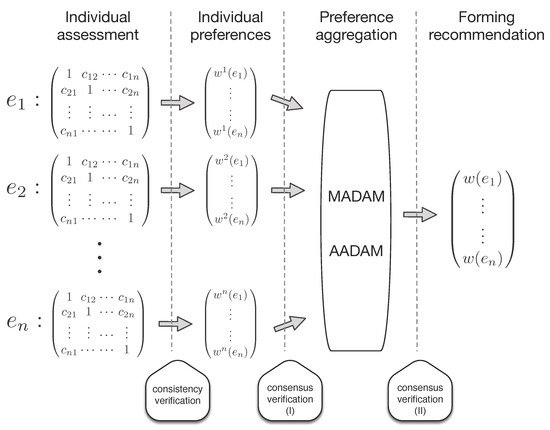
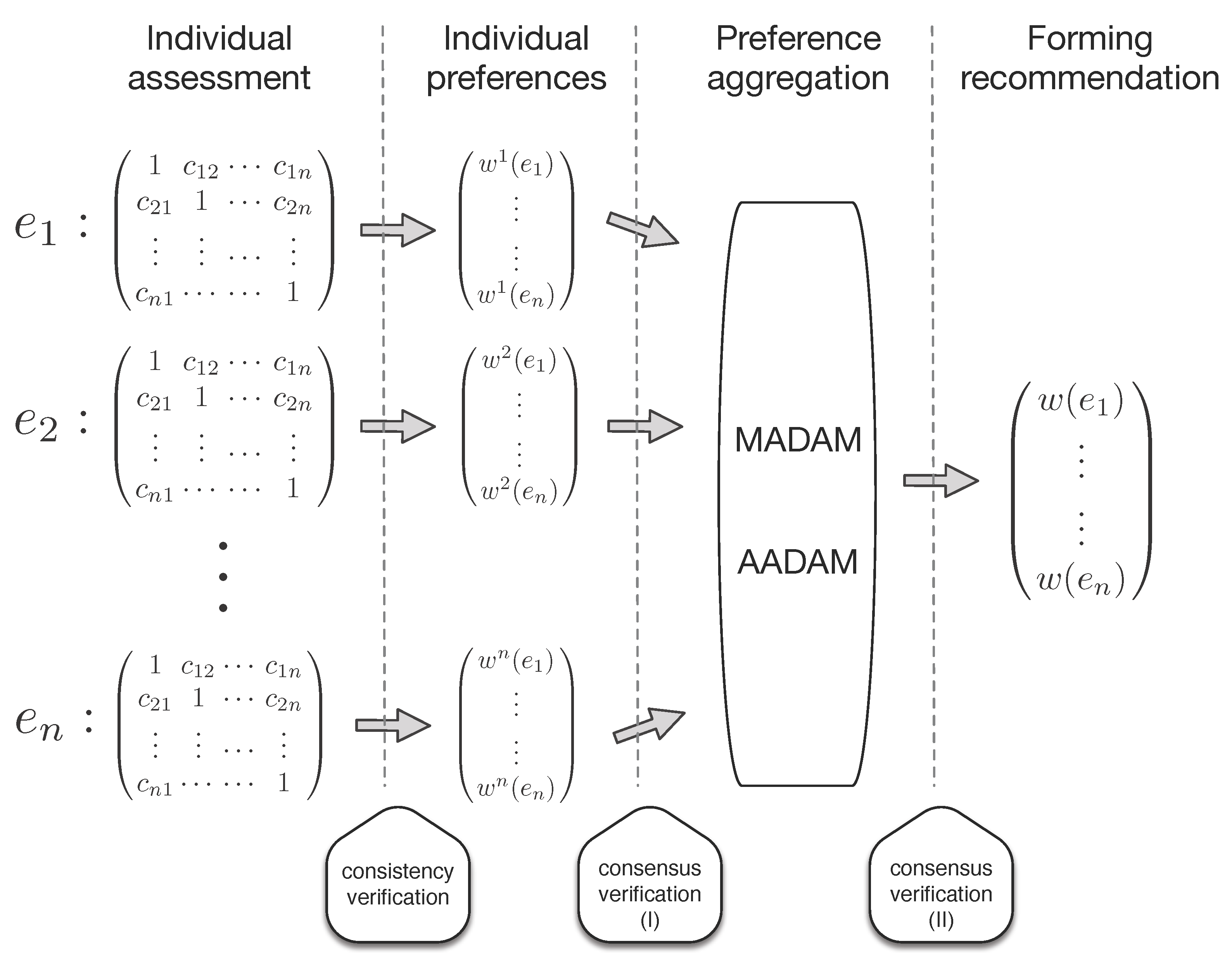
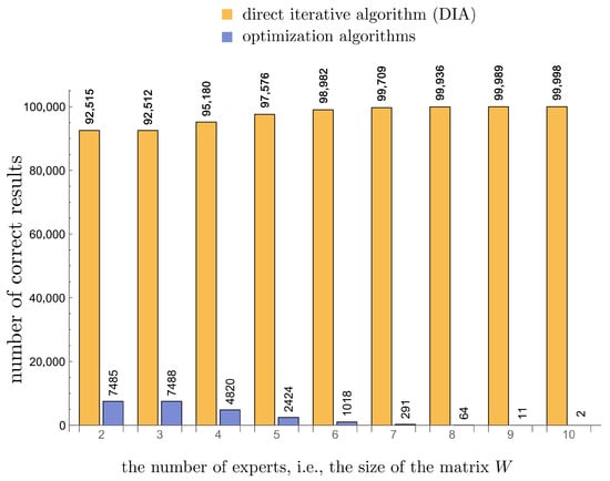
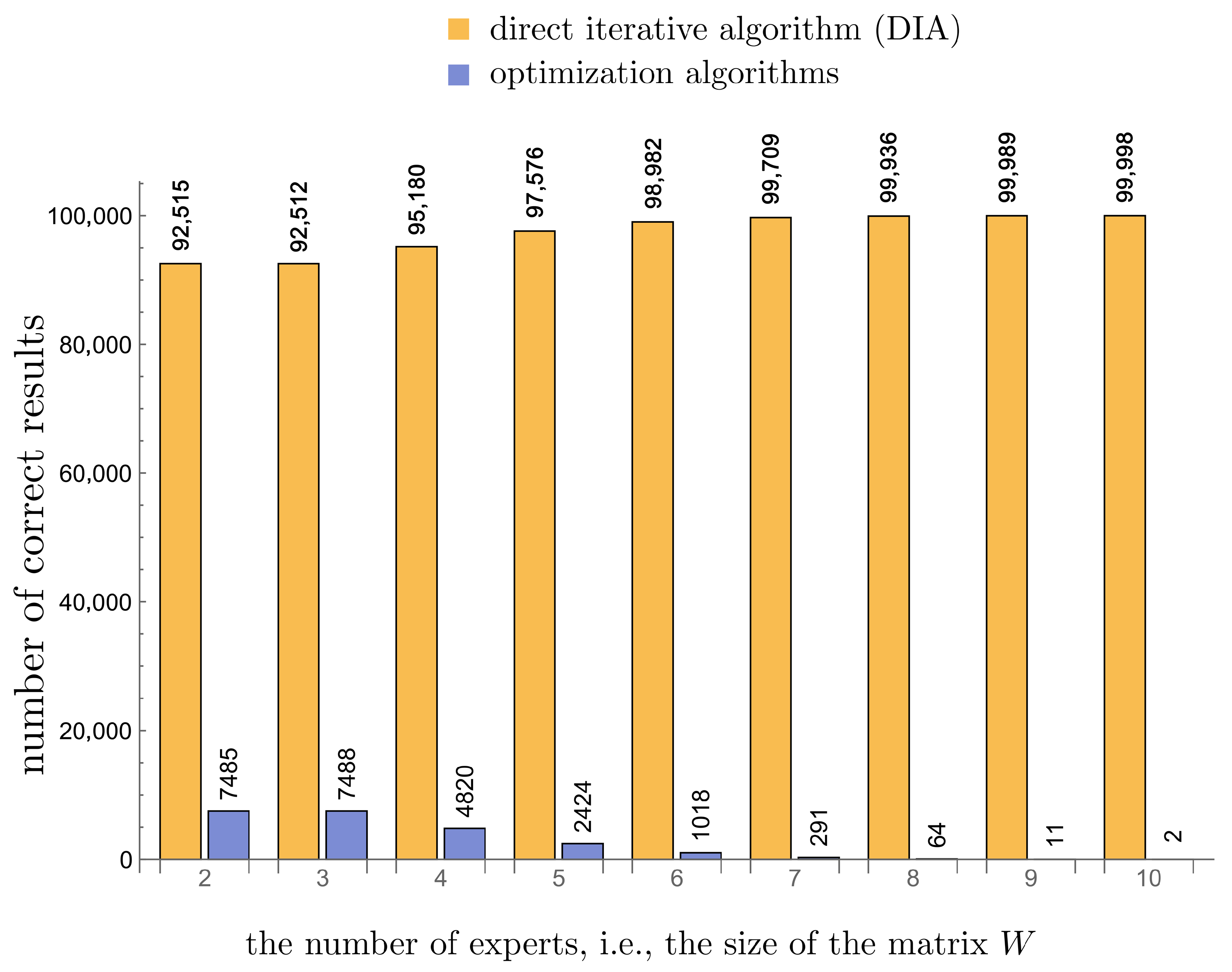
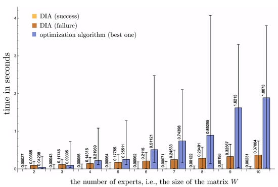
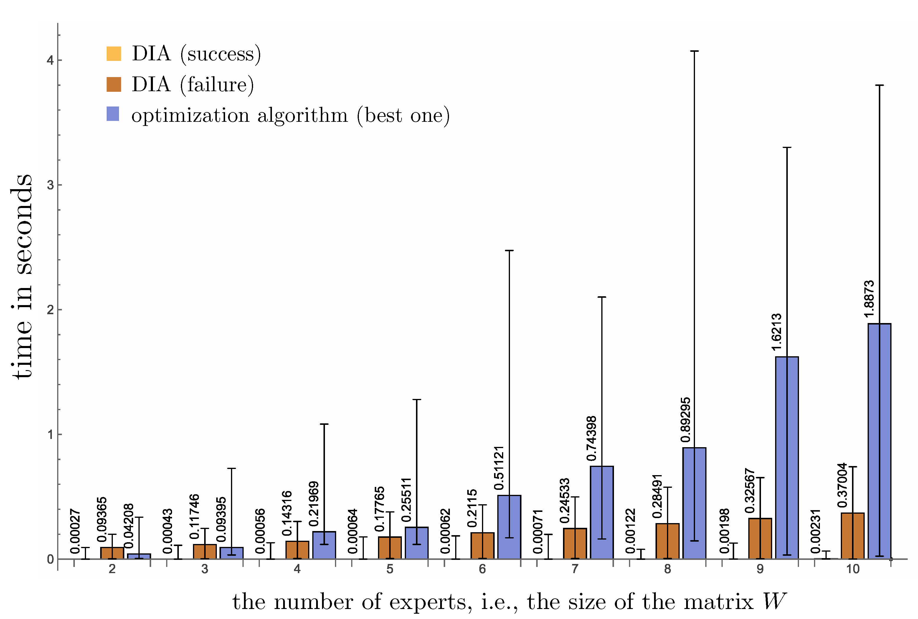
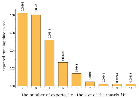
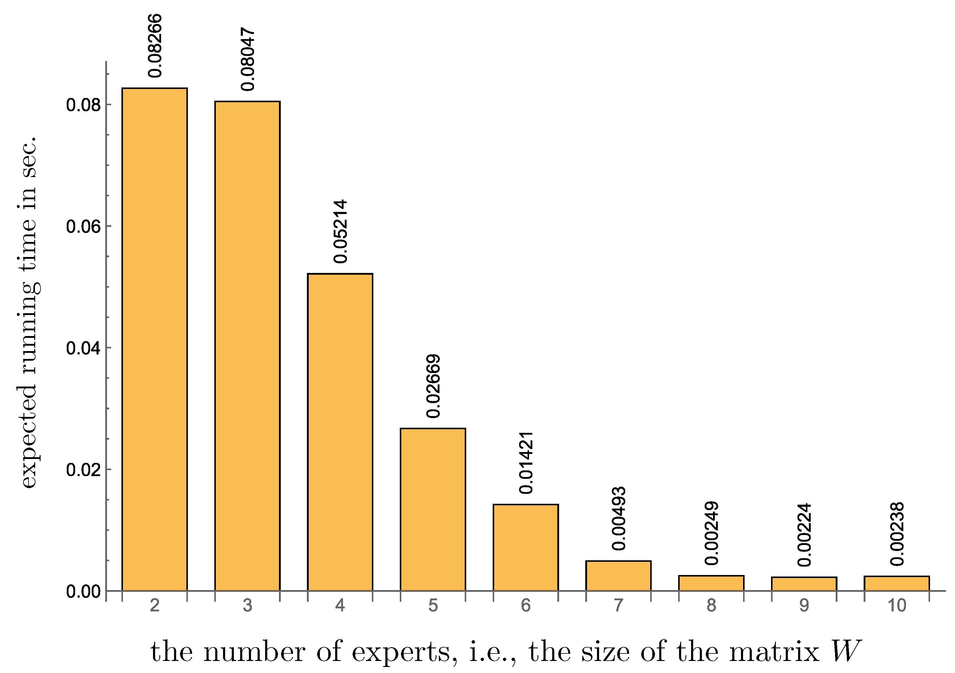
Disclaimer/Publisher’s Note: The statements, opinions and data contained in all publications are solely those of the individual author(s) and contributor(s) and not of MDPI and/or the editor(s). MDPI and/or the editor(s) disclaim responsibility for any injury to people or property resulting from any ideas, methods, instructions or products referred to in the content. |
© 2026 by the authors. Licensee MDPI, Basel, Switzerland. This article is an open access article distributed under the terms and conditions of the Creative Commons Attribution (CC BY) license.