Article

Color Image Storage and Retrieval via Sliding Mode Control of Quaternion-Valued Neural Networks

Department of Mathematics, Jinan University, Guangzhou 510632, China
*
Author to whom correspondence should be addressed.
Axioms 2026, 15(1), 72; https://doi.org/10.3390/axioms15010072
Submission received: 10 December 2025 / Revised: 14 January 2026 / Accepted: 18 January 2026 / Published: 20 January 2026
(This article belongs to the Special Issue Complex Networks and Dynamical Systems)

Abstract

This paper investigates the global polynomial synchronization (GPS) problem for quaternion-valued neural networks (QVNNs) featuring proportional delay, parameter uncertainty, and external disturbance. A combined approach of sliding mode control (SMC) and a non-separation strategy is adopted to achieve this goal. First, an integral-type sliding surface is designed for the system. Then, by constructing a delay-free Lyapunov functional and leveraging the properties of the quaternion vector norm and inequality techniques, sufficient conditions are derived to achieve GPS for the sliding mode dynamics. Furthermore, both a SMC law and an adaptive SMC law are designed, with a reachability analysis confirming that the system trajectories reach the predefined sliding surface in finite time. Finally, numerical examples with graphical analysis are provided to verify the obtained results, along with their application in color image pattern storage and retrieval.

1. Introduction

Over recent decades, neural networks (NNs) have demonstrated significant potential in solving complex nonlinear problems. This capability stems from their powerful information processing. Their success is evidenced by applications in diverse fields like pattern recognition [1], intelligent control [2], medical diagnosis [3,4], and biological modeling [5]. Both real-valued neural networks (RVNNs) [6,7,8,9] and complex-valued neural networks (CVNNs) [10,11,12] have yielded positive results in theoretical analysis and engineering applications. However, traditional real-valued or complex-valued models exhibit limitations in processing efficiency and structural representation when dealing with high-dimensional data tasks, such as 3D motion and color image processing. In 1843, Hamilton proposed quaternions, which consist of one real component and three imaginary components and do not satisfy the commutative law of multiplication. This is one of the reasons why research on quaternions progressed slowly after their introduction. In 2010, quaternions were first introduced into neural network models by Isokawa. Leveraging their algebraic structure, quaternion systems can effectively tackle numerous high-dimensional data issues in practical scenarios, such as 3D wind field forecasting [13] and computer graphics [14]. A prominent application is color image processing [15], where the red, green, and blue channels can be naturally mapped to the three imaginary parts of a quaternion. This representation enables holistic processing, often yielding superior performance compared to traditional real/complex-valued systems [16]. This structural advantage enables QVNNs to demonstrate potential efficiency in color image storage and retrieval tasks [17]. Therefore, in-depth research on the dynamic behaviors of QVNNs holds significant theoretical and practical value.
To date, various synchronization modes in NNs have been extensively studied, including quasi-synchronization [18,19], projective synchronization [20,21], exponential synchronization, and asymptotic synchronization [14,16,22]. In ref. [6], the global exponential synchronization (GES) and GPS were investigated for NNs with and without proportional delay. This study first proposed GPS and demonstrated its slower convergence rate compared to GES. This characteristic makes GPS not only more suitable for practical modeling but also an effective solution to the issue of excessively fast convergence inherent in GES. Consequently, GPS has attracted growing scholarly attention [10,11,12,23]. For instance, Zhang and Zhou [12] employed Lyapunov–Krasovskii functionals and linear matrix inequalities (LMI) to investigate GPS in CVNNs with multiple delays and impulses. In ref. [10], two adaptive controllers were designed, accompanied by the development of a lemma applicable to differential inequality systems with proportional delay, which collectively achieved adaptive GPS for memristive CVNNs. These achievements have laid the foundation for research on GPS and provided motivation for its extension to the QVNNs.
Despite the notable advantages of QVNNs in processing high-dimensional data, the non-commutativity of quaternion multiplication poses fundamental challenges to their dynamical analysis. Early studies often employed decomposition methods, transforming the system into four RVNNs or two CVNNs for separate investigation. For instance, Liu et al. [24] decomposed QVNNs into two complex-valued systems and constructed a Lyapunov function using Hermitian matrices to analyze the global μ -stability of QVNNs with unbounded delays. In ref. [16], a class of memristor-based quaternion-valued fuzzy neural networks with impulsive and time-varying delays was decomposed into four RVNNs. Based on the Halanay differential inequality, a new lemma applicable to delayed impulsive systems was proposed, and criteria for GES of the system were established. However, such methods not only significantly increase computational complexity but also lead to information loss and result deviation because they disrupt the intrinsic algebraic structure of quaternions. To overcome these limitations, many researchers have focused on directly analyzing the dynamical characteristics of QVNNs using non-decomposition methods [14,22,25]. For example, in ref. [25], leveraging the homeomorphic mapping theorem and Lyapunov theory, the global robust stability of equilibrium points (EPs) for delayed QVNNs with parameter uncertainty was derived using quaternion modulus inequality techniques. In ref. [22], based on quaternion theory and inequality techniques, two novel Lyapunov functionals were constructed to directly analyze the GES and GAS of the inertial QVNNs. In ref. [26], by introducing an improved 1-norm method and adopting a direct analysis approach, the GES of quaternion-valued memristive Cohen–Grossberg neural networks was studied. Therefore, investigating the dynamic behaviors of delayed QVNNs within a non-decomposition framework is both highly important and intriguing.
Time delay constitutes another critical factor in neural network modeling. Traditional research has predominantly focused on bounded delays [7,8,9,25,26]. However, such models are limited in characterizing real-world processes with continuously increasing delays, such as network congestion and signal accumulation. Consequently, scholars have gradually shifted their attention to unbounded delays [23,24,27,28,29,30,31], among which proportional delay is a typical form. Since proportional delay was first introduced into cellular neural networks in [30], a series of advances have been made in related studies. For example, ref. [31] investigated the projective synchronization of a class of inertial quaternion neural networks with proportional delay by constructing a Lyapunov function with adjustable parameters. Meanwhile, ref. [23] studied the polynomial synchronization of quaternion-valued fuzzy cellular neural networks with proportional delay by constructing a delay-free Lyapunov function. It is noteworthy that most of the aforementioned studies are based on idealized assumptions where system parameters are precisely known and free from external disturbances. In practice, however, parameter uncertainties and external disturbances are ubiquitous. The coupling effects of these factors within proportional delay systems have not been sufficiently studied, and the corresponding dynamic and control analyses remain notably underdeveloped.
For such composite uncertain systems, SMC is regarded as an effective strategy due to its strong robustness against parameter perturbations and external disturbances, finite-time convergence, and ease of physical implementation. Its core idea involves designing a sliding surface and a corresponding discontinuous control law to drive and confine the system states to this surface within finite time. In recent years, SMC theory has advanced significantly in synchronization. For example, ref. [32] combined nonsingular terminal sliding mode with adaptive neural networks for finite-time tracking in rehabilitation robots. Meanwhile, ref. [33] designed robust controllers for multi-input multi-output systems to achieve fixed-time synchronization. However, existing achievements in applying SMC to NNs synchronization are mostly concentrated on real-valued or complex-valued systems [34,35,36,37,38,39]. These studies often rely on system decomposition [37,38], lack completeness in the reachability analysis of the sliding surface [34], or introduce strong conservatism [35]. Current research on sliding mode synchronization control for QVNNs remains relatively limited. Although a preliminary exploration of sliding mode synchronization for delayed QVNNs with disturbance was presented in [40], a systematic investigation into the GPS of QVNNs subject to parameter uncertainty, external disturbance, and proportional delay based on the SMC method within a non-decomposition framework remains an open research problem.
Motivated by the above discussions, this paper aims to propose a SMC strategy investigate the GPS of QVNNs with parameter uncertainty, external disturbances, and proportional delays. This significant subject holds some measure of academic and practical importance, and as a result is accompanied by intrinsic difficulties. To achieve this goal, the primary challenges are listed below: (i) How to construct a systematic analytical framework to achieve GPS of QVNNs subject to parameter uncertainty, external disturbance, and proportional delay? (ii) How to establish synchronization criteria independent of proportional delay, thereby ensuring the universality of the obtained theoretical results? (iii) How to design an effective SMC to ensure the synchronization of QVNNs, particularly in scenarios where the upper bounds of disturbances are unknown? To address these core challenges, the main contributions of this work are as follows:
(1)
For the first time, the SMC strategy is introduced to address GPS for QVNNs with uncertain parameter, external disturbance, and proportional delay. An integral-type sliding surface and a SMC law are designed to effectively suppress external disturbance. Furthermore, an adaptive SMC law is proposed for the scenario where the upper bound of the disturbance is unknown, thereby enhancing the practicality of the control strategy.
(2)
In contrast to [34], this paper not only analyzes the accessibility of the sliding surface but also integrates SMC and the integral characteristics of the sliding surface to derive synchronization criteria that are independent of proportional delays.
(3)
Unlike the decomposition methods in [16,24], we use a direct analysis method that preserves the original system structure and reduces computational complexity.
(4)
Two numerical experiments are conducted to validate the correctness and effectiveness of the proposed method, along with a demonstration of its practical value in color image pattern storage and retrieval tasks.
Notations: R and R + denote the sets of all real and nonnegative numbers, respectively. Q denotes the set of all quaternions. The set of all ϑ -dimensional quaternion is denoted by Q ϑ . Q ϑ × ϑ represents the set of all ϑ × ϑ quaternion matrices. For y = y R + i y I + j a J + k y K Q , where y S R , S Ξ = { R , I , J , K }, the conjugate of y is denoted by y = y R i y I j y J k y K , and the module of y is written as y = y y = ( y R ) 2 + ( y I ) 2 + ( y J ) 2 + ( y K ) 2 , y 1 = | y R | + | y I | + | y J | + | y K | , for each y ( t ) = ( y 1 ( t ) , y 2 ( t ) , , y ϑ ( t ) ) Q ϑ , y ( t ) 0 = max p Π { y p ( t ) } , and H p + = sup t R H p ( t ) . Here i , j and k are standard imaginary units in Q which obey the Hamilton rules: i j = j i = k , j k = k j = i , k i = i k = j and i 2 = j 2 = k 2 = 1 . Π denotes the set of { 1 , 2 , , ϑ } .

2. Preliminaries

Consider QVNNs with uncertain parameters, external disturbance and proportional delay as the drive system,
m ˙ p ( t ) = θ p m p ( t ) + q = 1 ϑ α p q + Δ α p q ( t ) f q ( m q ( t ) ) + q = 1 ϑ β p q + Δ β p q ( t ) g q ( m q ( κ q t ) ) + J p ( t ) ,
and corresponding response system,
n ˙ p ( t ) = θ p n p ( t ) + q = 1 ϑ α p q + Δ α p q ( t ) f q ( n q ( t ) ) + q = 1 ϑ β p q + Δ β p q ( t ) g q ( n q ( κ q t ) ) + J p ( t ) + δ p H p ( t ) + U p ( t ) ,
where p Π , t t 0 ; m p ( t ) Q , n p ( t ) Q denote the state of the p-th neuron of QVNNs (1) and (2), respectively; θ p R is self-feedback coefficient; α p q Q , β p q Q represent the connection weights; Δ α p q ( t ) Q , Δ β p q ( t ) Q denote the bounded uncertain parameters; f q ( · ) , g q ( · ) Q are the activation functions; κ q is the proportional delay factor of qth neuron and satisfy 0 < κ q < 1 and κ q t = t ( 1 κ q ) t ; J p ( t ) Q denotes the external input; H p ( t ) Q represents the external disturbance; δ p R is a given constant, and U p ( t ) is the control input.
The initial conditions for systems (1) and (2) are given, respectively, by m p ( ι ) = m ^ p ( ι ) and n p ( ι ) = n ^ p ( ι ) for ι [ κ ˜ t 0 , t 0 ] , where κ ˜ = min q Π { κ q } , and m ^ p ( ι ) , n ^ p ( ι ) C ( [ κ ˜ t 0 , t 0 ] , Q ) .
Denote E p ( t ) = n p ( t ) m p ( t ) . Then, through systems (1) and (2), the error system can be calculated as
E ˙ p ( t ) = θ p E p ( t ) + q = 1 ϑ α p q + Δ α p q ( t ) F q ( E q ( t ) ) + q = 1 ϑ β p q + Δ β p q ( t ) G q ( E q ( κ q t ) ) + δ p H p ( t ) + U p ( t ) ,
where F q ( E q ( t ) ) = f q ( n q ( t ) ) f q ( m q ( t ) ) , G q ( E q ( κ q t ) ) = g q ( n q ( κ q t ) ) g q ( m q ( κ q t ) ) , the initial conditions of system (3) are E p ( ι ) = E ^ p ( ι ) = n ^ p ( ι ) m ^ p ( ι ) , ι [ κ ˜ t 0 , t 0 ] .
Remark 1.
As a type of monotonically increasing and unbounded time-varying delay, proportional delay is distinct from constant delays [41], bounded time-varying delays [26], and distributed delays [42]. It simultaneously exhibits time dependence, unbounded growth, and low conservatism. This form of delay is prevalent in real-world applications such as routing decision-making and Quality-of-Service assurance in communication networks [43].
Definition 1
([44]). Systems (1) and (2) are said to be globally polynomially synchronized if there exist positive constants Υ m ^ , n ^ and ξ such that
n ( t ) m ( t ) 0 Υ m ^ , n ^ 1 + t 1 + t 0 ξ ,
where ξ denotes the polynomial synchronous decay rate, and Υ m ^ , n ^ represents a positive constant that depend on the initial functions m ^ , n ^ , in which m ^ ( ι ) = ( m ^ p ( ι ) ) , n ^ ( ι ) = ( n ^ p ( ι ) ) C ( [ κ ˜ t 0 , t 0 ] , Q ϑ ) .
Definition 2.
For χ Q , the sign function of χ is defined as χ = s i g n ( χ R ) + i s i g n ( χ I ) + j s i g n ( χ J ) + k s i g n ( χ K ) .
Lemma 1
([45]). Let χ ( t ) Q , then
χ ( t ) χ ( t ) + χ ( t ) χ ( t ) = 2 χ ( t ) 1 2 χ ( t ) ,
D + χ ( t ) χ ( t ) + χ ( t ) χ ( t ) = χ ( t ) χ ˙ ( t ) + χ ˙ ( t ) χ ( t ) .
Lemma 2
([46]). If ϖ , η Q , then
ϖ η + η ϖ 2 ϖ η , ϖ η + η ϖ ϖ ϖ + η η .
Remark 2.
For any ϖ , η , ϱ Q ,
( ϖ η ) ϱ + ( ϖ η ) ϱ = ϖ ϖ ϱ ϱ + η η .
Lemma 3.
For p Π , let v p ( t ) : R + R be a set of locally Lipschitz continuous functions, where Π is a finite index set. Define
V ( t ) = max p Π v p ( t ) .
Then, the upper right Dini derivative of V ( t ) satisfies
D + V ( t ) = max p A ( t ) D + v p ( t ) ,
where A ( t ) = { p Π : v p ( t ) = V ( t ) } is the set of active indices at time t.
Proof. 
Fix t 0 , for any p A ( t ) and h > 0 , we have v p ( t ) = V ( t ) and V ( t + h ) v p ( t + h ) . Hence,
V ( t + h ) V ( t ) h v p ( t + h ) v p ( t ) h .
Taking the upper limit as h 0 + yields D + V ( t ) D + v p ( t ) for all p A ( t ) . Therefore,
D + V ( t ) max p A ( t ) D + v p ( t ) .
For sufficiently small h > 0 , choose p h Π such that V ( t + h ) = v p h ( t + h ) . Since v p h ( t ) V ( t ) , then
V ( t + h ) V ( t ) h = v p h ( t + h ) V ( t ) h v p h ( t + h ) v p h ( t ) h ,
Taking the upper limit as h 0 + gives
D + V ( t ) lim sup h 0 + v p h ( t + h ) v p h ( t ) h .
Since Π is finite, there exists a sequence h k 0 + such that p h k = p is constant. Thus,
D + V ( t ) lim sup k v p ( t + h k ) v p ( t ) h k D + v p ( t ) .
Moreover, by continuity, v p ( t ) = lim k v p ( t + h k ) = lim k V ( t + h k ) = V ( t ) , which implies p A ( t ) . Consequently,
D + V ( t ) D + v p ( t ) max p A ( t ) D + v p ( t ) .
Combining (4) and (5) completes the proof. □
Assumption 1.
For any q Π , the expression of activation function f q ( · ) , g q ( · ) satisfies f q ( · ) = f q ( · ) R + i f q ( · ) I + j f q ( · ) J + k f q ( · ) K , g q ( · ) = g q ( · ) R + i g q ( · ) I + j g q ( · ) J + k g q ( · ) K , and there exist L q f , L q g R + such that for each x , y Q ,
f q ( y ) f q ( x ) L q f y x ,
g q ( y ) g q ( x ) L q g y x .
Assumption 2.
Δ α p q ( t ) = α ˜ p q λ p q ( t ) ,
Δ β p q ( t ) = β ˜ p q ϰ p q ( t ) ,
where α ˜ p q , β ˜ p q are constants, and λ p q ( t ) , ϰ p q ( t ) Q are uncertain functions such that λ p q ( t ) λ p q ( t ) 1 and ϰ p q ( t ) ϰ p q 1 .

3. Main Results

In this section, we first design a sliding mode surface from the drive-response and error systems, using an equivalent controller to achieve GPS of the sliding mode dynamics. Then, a SMC law is designed based on this surface, and its reachability is verified. To address unknown disturbance bounds, an adaptive SMC law is subsequently developed.
For convenience, the key notations employed in this section are summarized as follows: ξ denotes the polynomial decay rate; H p + = sup t R H p ( t ) represents the upper bound of the external disturbance; and L q f and L q g are the Lipschitz constants of the activation functions f q ( · ) and g q ( · ) , respectively.
The sliding-mode surface function is constructed as
χ p ( t ) = E p ( t ) + 0 t θ p E p ( s ) q = 1 ϑ α p q F q ( E q ( s ) ) q = 1 ϑ β p q G q ( E q ( κ q s ) ) + ζ p E p ( s ) d s ,
where ζ p > 0 denotes the gain coefficient.
Then, combining (3) with (6), we obtain
χ p ( t ) = E p ( t ) + 0 t ( δ p H p ( s ) + U p ( s ) + ζ p E p ( s ) + q = 1 ϑ Δ α p q ( s ) F q ( E q ( s ) ) + q = 1 ϑ Δ β p q G q ( E q ( κ q s ) ) E ˙ p ( s ) ) d s .
By applying SMC theory and the sliding surface existence condition χ p ( t ) = χ ˙ p ( t ) = 0 , the equivalent control law is derived as
U p ( t ) = ζ p E p ( t ) q = 1 ϑ Δ α p q ( t ) F q ( E q ( t ) ) q = 1 ϑ Δ β p q G q ( E q ( κ q t ) ) δ p H p ( t ) .
Substituting (8) into (3) yields the sliding mode dynamics as
E ˙ p ( t ) = θ p E p ( t ) ζ p E p ( t ) + q = 1 ϑ α p q F q ( E q ( t ) ) + q = 1 ϑ β p q G q ( E q ( κ q t ) ) .
Theorem 1.
Under the Assumption 1, if a positive constant ξ satisfies
2 ( θ p + ζ p ) + 2 ξ + q = 1 ϑ ( α p q 2 + β p q 2 ) + ϑ ( L q f ) 2 + ϑ ( L q g ) 2 < 0 ,
then, the sliding mode dynamics (9) achieve GPS, and the systems (1) and (2) can be synchronized under the SMC (8).
Proof. 
Define for each p Π ,
v p ( t ) = E p ( t ) E p ( t ) 1 + t 1 + t 0 2 ξ ,
and construct the Lyapunov function as
V ( t ) = max p Π { v p ( t ) } .
Note that this is equivalent to
V ( t ) = max p Π { E p ( t ) E p ( t ) } 1 + t 1 + t 0 2 ξ .
By Lemma 3, we have
D + V ( t ) = max p A ( t ) D + v p ( t ) ,
where A ( t ) = { p Π : v p ( t ) = V ( t ) } . Under the Lemma 2, the upper right Dini derivative of V ( t ) along the trajectories of (9) is given by
D + V ( t ) = max p A ( t ) E ˙ p ( t ) E p ( t ) + E p ( t ) E ˙ p ( t ) + E p ( t ) E p ( t ) 2 ξ 1 + t 1 + t 1 + t 0 2 ξ = max p A ( t ) E ˙ p ( t ) E p ( t ) + E p ( t ) E ˙ p ( t ) + E p ( t ) E p ( t ) 2 ξ 1 + t 1 + t 1 + t 0 2 ξ = max p A ( t ) { θ p E p ( t ) ζ p E p ( t ) + q = 1 ϑ α p q F q ( E q ( t ) ) + q = 1 ϑ β p q G q ( E q ( κ q t ) ) E p ( t ) + E p ( t ) θ p E p ( t ) ζ p E p ( t ) + q = 1 ϑ α p q F q ( E q ( t ) ) + q = 1 ϑ β p q G q ( E q ( κ q t ) ) + E p ( t ) E p ( t ) 2 ξ 1 + t } 1 + t 1 + t 0 2 ξ = max p A ( t ) { ( θ p + ζ p ) E p ( t ) E p ( t ) E p ( t ) ( θ p + ζ p ) E p ( t ) + q = 1 ϑ α p q F q ( E q ( t ) ) E p ( t ) + E p ( t ) α p q F q ( E q ( t ) ) + q = 1 ϑ β p q G q ( E q ( κ q t ) ) E p ( t ) + E p ( t ) β p q G q ( E q ( κ q t ) ) + E p ( t ) E p ( t ) 2 ξ 1 + t } 1 + t 1 + t 0 2 ξ max p A ( t ) { ( θ p + ζ p ) E p ( t ) E p ( t ) E p ( t ) ( θ p + ζ p ) E p ( t ) + q = 1 ϑ α p q α p q E q ( t ) E p ( t ) + F q ( E q ( t ) ) F q ( E q ( t ) ) + q = 1 ϑ β p q β p q E q ( t ) E p ( t ) + G q ( E q ( κ q t ) ) G q ( E q ( κ q t ) ) + E p ( t ) E p ( t ) 2 ξ 1 + t } 1 + t 1 + t 0 2 ξ .
Based on Assumption 1, we yield
D + V ( t ) max p A ( t ) { 2 ( θ p + ζ p ) E p ( t ) E p ( t ) + q = 1 ϑ α p q 2 E p ( t ) E p ( t ) + ϑ L f 2 E p ( t ) E p ( t ) + q = 1 ϑ β p q 2 E p ( t ) E p ( t ) + ϑ L g 2 E p ( t ) E p ( t ) + E p ( t ) E p ( t ) 2 ξ 1 + t } 1 + t 1 + t 0 2 ξ max p Π { [ 2 ( θ p + ζ p ) + 2 ξ + q = 1 ϑ ( α p q 2 + β p q 2 ) + ϑ ( L q f ) 2 + ϑ ( L q g ) 2 ] E p ( t ) E p ( t ) } 1 + t 1 + t 0 2 ξ 0 .
Obviously, we can obtain V ( t ) V ( t 0 ) , which indicates
max p Π { E p ( t ) E p ( t ) } 1 + t 1 + t 0 2 ξ V ( t 0 ) .
This is equivalent to
E ( t ) E ( t ) 0 V ( t 0 ) 1 + t 1 + t 0 2 ξ .
Consequently,
E ( t ) 0 V ( t 0 ) 1 + t 1 + t 0 ξ .
Let Υ m ^ , n ^ = V ( t 0 ) , we have
n ( t ) m ( t ) 0 Υ m ^ , n ^ 1 + t 1 + t 0 ξ .
Therefore, according to Definition 1, the sliding mode dynamics (9) achieve GPS, which implies that systems (1) and (2) are synchronized. □
Remark 3.
In this paper, by constructing a delay-free Lyapunov functional incorporating state variable derivatives, designing an integral-type sliding surface and corresponding sliding mode controller for the system, selecting the infinity norm as the quaternion vector norm, and employing a non-decomposition approach, we not only establish sufficient conditions for GPS of the sliding mode dynamics, but also ensure the entire proof process remains concise and efficient.
Remark 4.
The LMI method relies heavily on matrix representations and linear transformations of system dynamics. For complex NNs, its applicability is often limited, and it tends to increase the computational dimensionality. This issue is particularly pronounced for QVNNs, where decomposition-based LMI approaches incur substantial computational complexity [47]. In contrast, the method proposed in this paper imposes a lighter computational burden compared to matrix-based operations. Moreover, the complexity of its stability conditions does not scale sharply with the number of neurons ϑ. As a result, it offers favorable scalability when applied to large-scale networks.
Remark 5.
L q f and L q g can be derived from the analysis of activation functions. The connection weights are determined by the network topology and can serve as design parameters in practice. The self-feedback coefficient θ p is an inherent system parameter, typically regarded as an adjustable design basis. ζ p acts as the feedback gain of the controller and is a key design variable that can be freely tuned. Once these parameters are chosen, the maximum achievable decay rate ξ max is determined by solving the equality condition associated with the inequality in Theorem 1. Although increasing ζ p raises ξ max , it also amplifies the linear feedback term ζ p E p ( t ) , potentially resulting in excessive control effort. Hence, a practical trade-off exists between the convergence speed and the control input magnitude.
To ensure the reachability of the sliding surface designed above, a SMC law is developed as
U p ( t ) = ζ p E p ( t ) Θ p ( t ) χ p ( t ) ,
where Θ p ( t ) = μ p + q = 1 ϑ L q f α ˜ p q E q ( t ) + q = 1 ϑ L q g β ˜ p q E q ( t ) .
Theorem 2.
Under the SMC law (13) and Assumptions 1 and 2, the state trajectories of the closed-loop (3) will converge to the sliding surface χ p ( t ) = 0 in finite time, where μ p > 2 δ p H p + .
Proof. 
Construct the following Lyapunov function
V ( t ) = max p Π { χ p ( t ) χ p ( t ) } .
Applying Lemma 3, we obtain
D + V ( t ) = max p A ( t ) D + [ χ p ( t ) χ p ( t ) ] ,
where A ( t ) = { p Π : χ p ( t ) χ p ( t ) = V ( t ) } .
Calculating the upper right Dini derivative of V ( t ) yields
D + V ( t ) = max p A ( t ) { χ ˙ p ( t ) χ p ( t ) + χ p ( t ) χ ˙ p ( t ) } = max p A ( t ) { ( δ p H p ( t ) + q = 1 ϑ Δ α p q ( t ) F q ( E q ( t ) ) + q = 1 ϑ Δ β p q G q ( E q ( κ q t ) ) Θ p ( t ) χ p ( t ) ) χ p ( t ) + χ p ( t ) ( δ p H p ( t ) + q = 1 ϑ Δ α p q ( t ) F q ( E q ( t ) ) + q = 1 ϑ Δ β p q G q ( E q ( κ q t ) ) Θ p ( t ) χ p ( t ) ) } .
According to Lemma 2 and Assumptions 1 and 2, we have
δ p H p ( t ) χ p ( t ) + χ p ( t ) ( δ p H p ( t ) ) 2 δ p H p ( t ) χ p ( t ) ,
q = 1 ϑ ( Δ α p q ( t ) F q ( E q ( t ) ) χ p ( t ) + χ p ( t ) Δ α p q ( t ) F q ( E q ( t ) ) ) 2 q = 1 ϑ Δ α p q ( t ) F q ( E q ( t ) ) χ p ( t ) 2 q = 1 ϑ L q f α ˜ p q E q ( t ) χ p ( t ) ,
q = 1 ϑ ( Δ β p q ( t ) G q ( E q ( κ q t ) ) χ p ( t ) + χ p ( t ) Δ β p q ( t ) G q ( E q ( κ q t ) ) ) 2 q = 1 ϑ Δ β p q ( t ) G q ( E q ( κ q t ) ) χ p ( t ) 2 q = 1 ϑ L q g β ˜ p q E q ( κ q t ) χ p ( t ) ,
Based on Lemma 1, we yield
D + V ( t ) 2 max p A ( t ) { δ p H p ( t ) χ p ( t ) + q = 1 ϑ L q f α ˜ p q E q ( t ) χ p ( t ) + q = 1 ϑ L q g β ˜ p q E q ( κ q t ) χ p ( t ) Θ p ( t ) χ p ( t ) 1 } 2 max p A ( t ) { δ p H p + χ p ( t ) + q = 1 ϑ L q f α ˜ p q E q ( t ) χ p ( t ) + q = 1 ϑ L q g β ˜ p q E q ( t ) χ p ( t ) Θ p ( t ) χ p ( t ) } max p A ( t ) { 2 δ p H p + χ p ( t ) 2 μ p χ p ( t ) } max p Π { 2 δ p H p + χ p ( t ) μ p χ p ( t ) } = ( μ p 2 δ p H p + ) χ p ( t ) .
When t > ( μ p 2 δ p H p + ) V ( 0 ) , χ p ( t ) = 0 . Therefore, the sliding surface χ p ( t ) = 0 is reached by the state trajectories of the error system (3) in finite time. □
Corollary 1.
In the absence of external disturbances and parameter uncertainties, and under mismatched external inputs, the following controller is designed to achieve synchronization between the drive-response systems (1) and (2)
U p ( t ) = ζ p E p ( t ) Δ J p μ p χ p ( t ) .
Under this condition, the dynamics of χ p ( t ) simplify to
χ ˙ p ( t ) = μ p χ p ( t ) .
Due to the fact that H p + in Theorem 2 is not always known a priori in practice, a corresponding adaptive SMC law is designed for system (3) as
U p ( t ) = ζ p E p ( t ) Θ ˜ p ( t ) χ p ( t ) ,
where Θ ˜ p ( t ) = μ p + q = 1 ϑ L q f α ˜ p q E q ( t ) + q = 1 ϑ L q g β ˜ p q E q ( t ) + δ p H ˜ P + ( t ) . Here, H ˜ P + ( t ) is the estimation of H p + , and the adaptive law is designed as
H ˜ ˙ p + ( t ) = δ p ρ χ p ( t ) ,
with H ˜ p + ( 0 ) = 0 , and ρ > 0 is a given scalar.
Theorem 3.
Suppose that the bound H p + is unknown. Under the adaptive SMC law (22) and Assumptions 1 and 2, the state trajectories of the closed-loop (3) will converge to the sliding surface χ p ( t ) = 0 in finite time, where μ p > 0 .
Proof. 
The Lyapunov function is designed as
V ( t ) = max p Π { χ p ( t ) χ p ( t ) + ρ ( H ˜ P + ( t ) H p + ) 2 } .
Similar to the proof of Theorem 2, one obtains
D + V ( t ) 2 max p Π { δ p H p ( t ) χ p ( t ) + q = 1 ϑ L q f α ˜ p q E q ( t ) χ p ( t ) + q = 1 ϑ L q g β ˜ p q E q ( κ q t ) χ p ( t ) Θ p ( t ) χ p ( t ) 1 + δ p ( H ˜ P + ( t ) H p + ) χ p ( t ) } 2 max p Π { δ p H p + χ p ( t ) + q = 1 ϑ L q f α ˜ p q E q ( t ) χ p ( t ) + q = 1 ϑ L q g β ˜ p q E q ( t ) χ p ( t ) Θ p ( t ) χ p ( t ) + δ p ( H ˜ P + ( t ) H p + ) χ p ( t ) } 2 max p Π { δ p H p + χ p ( t ) μ p χ p ( t ) δ p H ˜ P + ( t ) χ p ( t ) + δ p ( H ˜ P + ( t ) H p + ) χ p ( t ) } μ p max p Π { χ p ( t ) } .
Therefore, the error dynamics (3) will converge to the sliding surface χ p ( t ) = 0 within a finite time. □
Remark 6.
In ref. [34], reachability analysis is not performed on the sliding mode surface χ p ( t ) and, in [40], fails to discuss the scenario where the constraint H p + is unavailable. Accordingly, Theorem 2 introduces a SMC law to analyze the reachability, and Theorem 3 proposes an adaptive SMC law tailored for cases with unknown H p + .
Remark 7.
Refs. [37,38] utilized SMC based on the decomposition method to investigate the asymptotic synchronization and finite/fixed-time synchronization of CVNNs. However, the decomposition approach inevitably increases the number of subsystems to be analyzed, resulting in substantially higher computational complexity. Additionally, the decomposition process forces the non-commutative multiplication of quaternions into linear combinations of real and imaginary parts, which undermines the unique structure of the original model. In contrast, this paper integrates SMC with non-decomposition analysis, thereby avoiding the conservativeness introduced by decomposition and obtaining synchronization criteria that are easy to verify.

4. Numerical Examples

This section presents numerical examples with graphical analyses to demonstrate the efficacy of the proposed theoretical results, along with their application in color image pattern storage and retrieval.
Example 1.
Consider the following models:
m ˙ p ( t ) = θ p m p ( t ) + q = 1 2 α p q + Δ α p q ( t ) f q ( m q ( t ) ) + q = 1 2 β p q + Δ β p q ( t ) g q ( m q ( κ q t ) ) + J p ( t ) ,
n ˙ p ( t ) = θ p n p ( t ) + q = 1 2 α p q + Δ α p q ( t ) f q ( n q ( t ) ) + q = 1 2 β p q + Δ β p q ( t ) g q ( n q ( κ q t ) ) + J p ( t ) + δ p H p ( t ) + U p ( t ) .
The parameters are set as: p = 1 , 2 ; κ 1 = κ 2 = 0.5 ; θ 1 = 1 , θ 2 = 1.9 ; L 1 f = L 2 f = 0.3 ; L 1 g = L 2 g = 0.5 ; δ 1 = 0.5 , δ 2 = 0.55 ; ζ 1 = ζ 2 = 2.5 ; and J 1 = J 2 = 0 . The activation functions are defined as f ( · ) = 0.3 sin ( 3 · ) and g ( · ) = 0.5 sin ( 2 · ) . The external disturbances are given by:
H 1 ( t ) = 0.3 sin ( 3 t ) + 0.4 sin ( 2 t ) i + 0.8 cos ( t ) j + 0.8 sin ( t ) k , H 2 ( t ) = 0.3 sin ( 2 t ) + 0.4 sin ( 3 t ) i + 0.8 cos ( 3 t ) j + 0.8 sin ( 3 t ) k .
The connection weight matrices are selected as:
A = ( α p q ) 2 × 2 = 0.5 + 0.2 i + 0.2 j + 0.5 k 0.3 + 0.22 i 1.2 j + 0.6 k 0.5 0.31 i + 0.3 j + 0.42 k 0.3 + 0.1 i + 0.1 j 0.5 k ,
B = ( β p q ) 2 × 2 = 0.1 0.71 i + 0.5 j 0.41 k 0.3 + 0.41 i + 0.1 j + 0.4 k 0.6 0.2 i + 0.3 j 0.4 + 0.1 i 0.11 j 0.1 k .
The uncertain parameters are described by:
Δ α 11 ( t ) = 0.4 sin ( t ) 0.6 cos ( t ) i 0.4 cos ( t ) j + 0.4 sin ( t ) k , Δ α 12 ( t ) = 0.4 cos ( t ) + 0.4 sin ( t ) i 0.6 sin ( t ) j 0.4 sin ( t ) k , Δ α 21 ( t ) = 0.4 cos ( t ) 0.4 cos ( t ) i + 0.4 sin ( t ) j + 0.6 cos ( t ) k , Δ α 22 ( t ) = 0.6 sin ( t ) + 0.6 cos ( t ) i + 0.4 sin ( t ) j 0.4 cos ( t ) k , Δ β 11 ( t ) = 0.4 cos ( t ) + 0.6 cos ( t ) i + 0.4 sin ( t ) j 0.4 cos ( t ) k , Δ β 12 ( t ) = 0.6 cos ( t ) 0.4 cos ( t ) i + 0.4 cos ( t ) j + 0.4 sin ( t ) k , Δ β 21 ( t ) = 0.4 sin ( t ) 0.4 cos ( t ) i + 0.4 sin ( t ) j 0.6 sin ( t ) k , Δ β 22 ( t ) = 0.4 sin ( t ) + 0.6 cos ( t ) i + 0.6 sin ( t ) j + 0.4 cos ( t ) k .
The initial condition of drive system is [ m 1 ( 0 ) , m 2 ( 0 ) ] T = [ 0.8 0.6 i + 0.7 j 0.5 k , 0.7 + 0.9 i 0.8 j + 0.6 k ] T , and the initial condition of the response system is [ n 1 ( 0 ) , n 2 ( 0 ) ] T = [ 0.3 0.2 i + 0.4 j 0.1 k , 0.1 + 0.2 i 0.3 j + 0.1 k ] T .
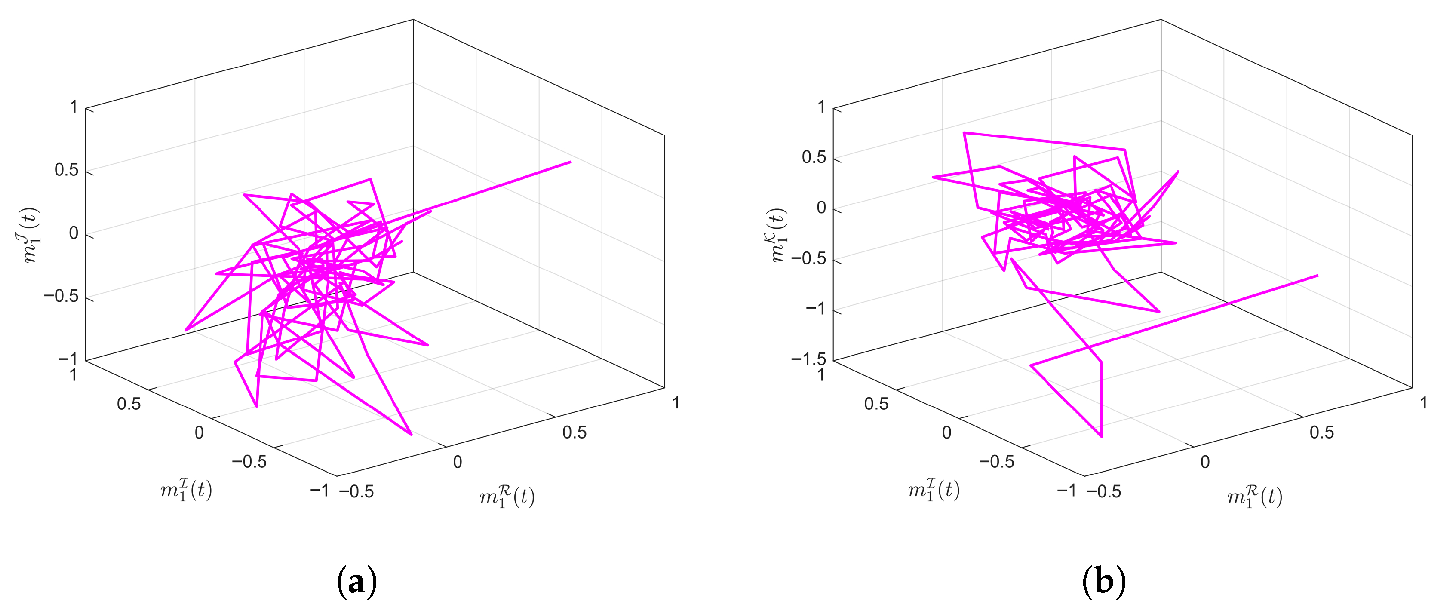
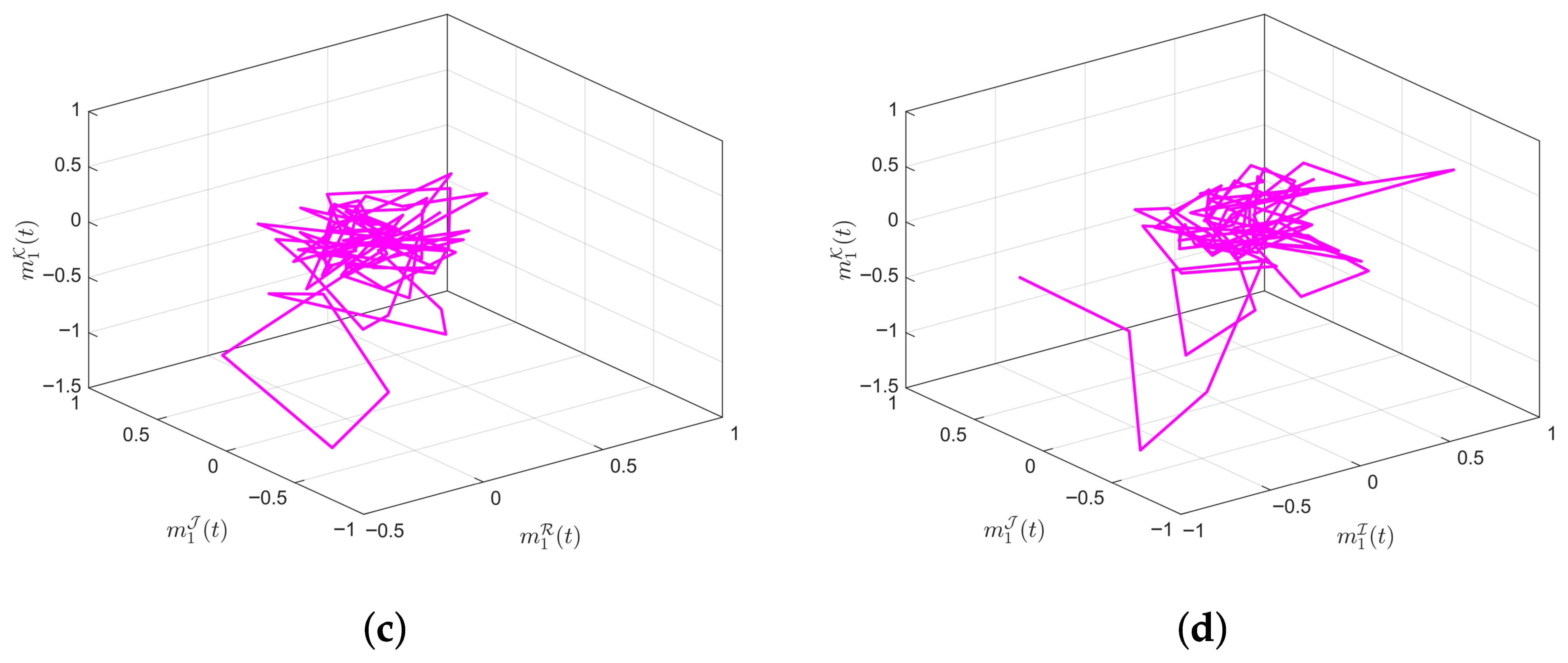
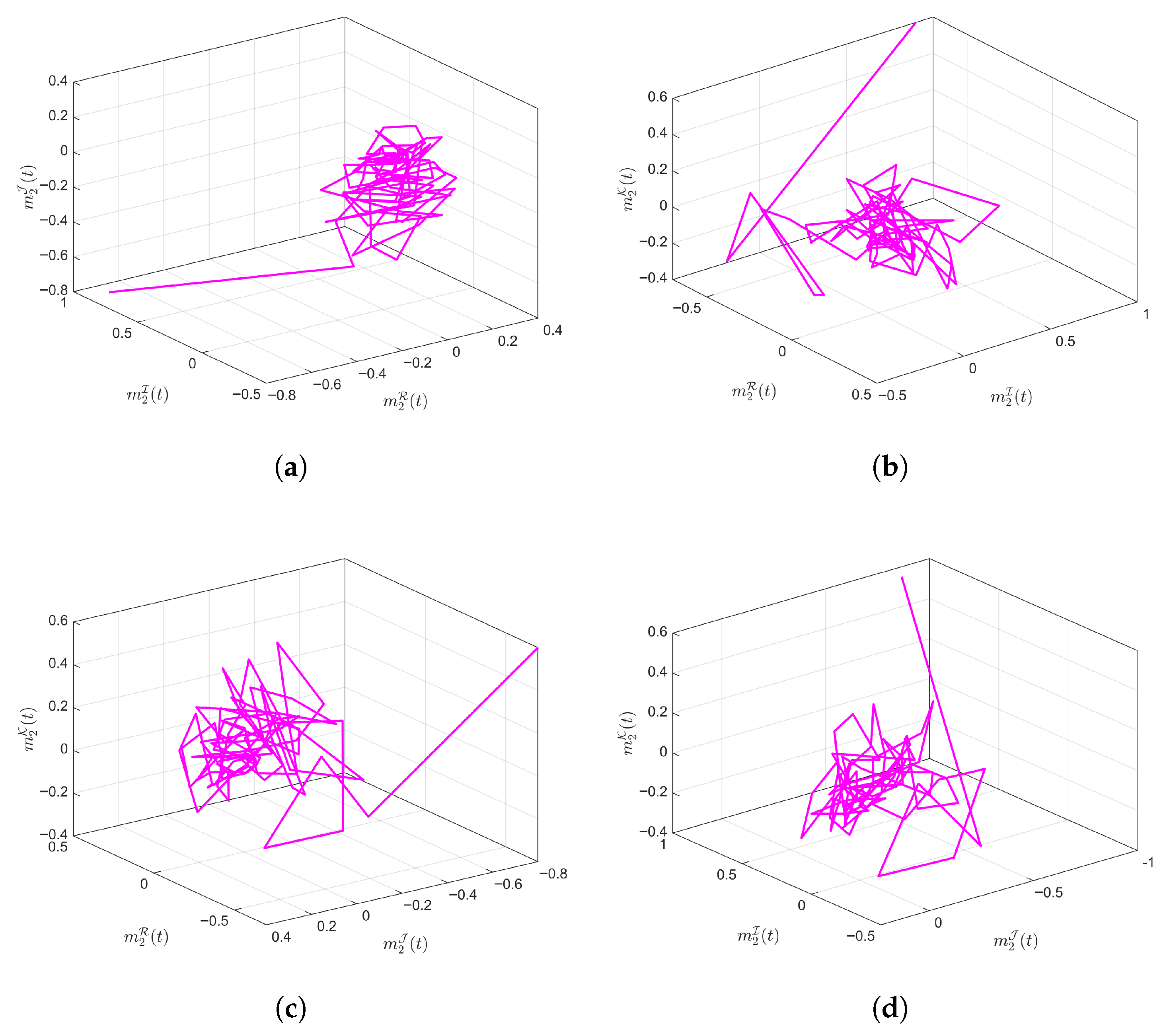
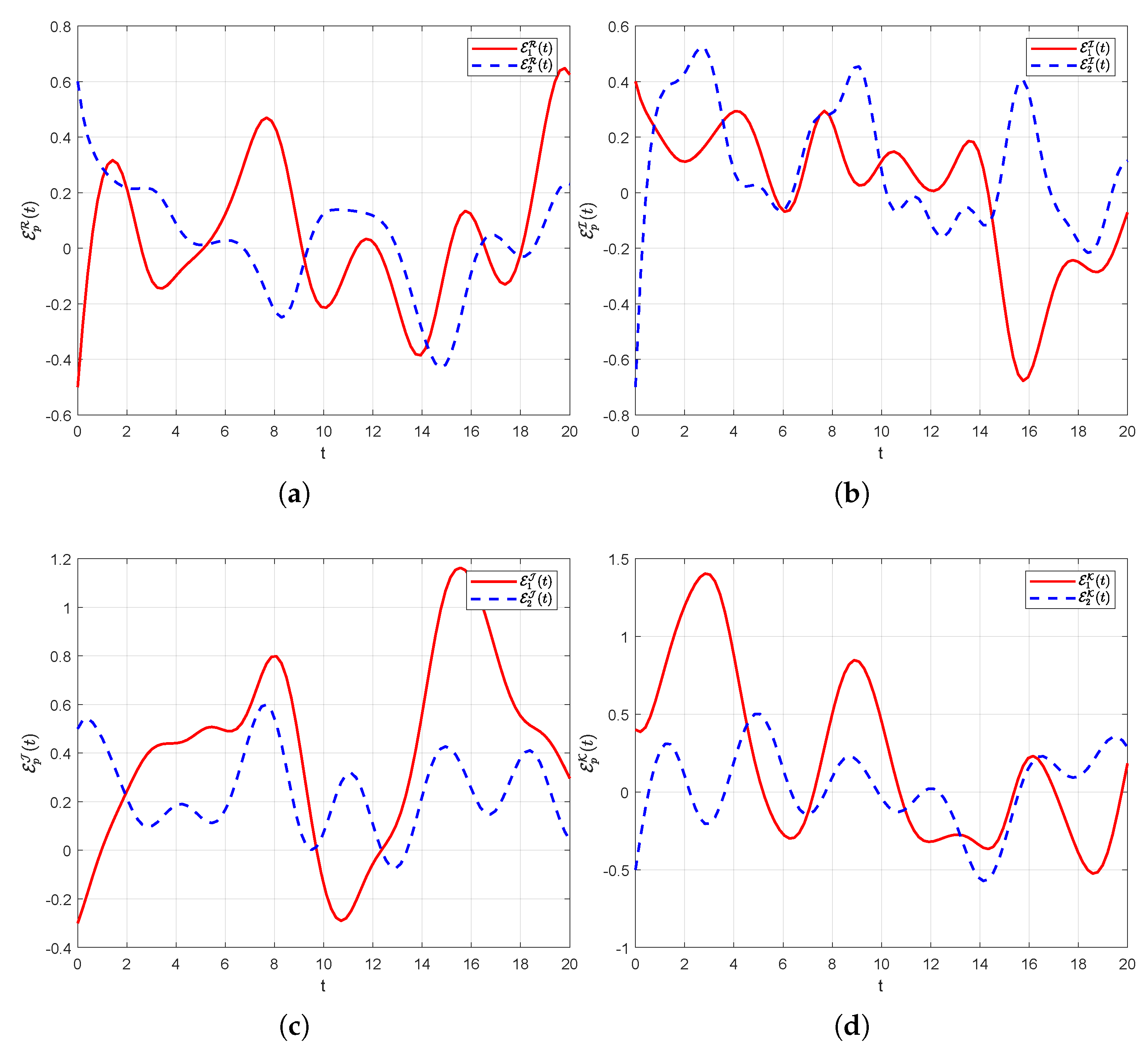
Figure 1 and Figure 2 display the chaotic attractors of the first and second neurons, respectively, for the drive system (26) under different initial conditions. In the absence of the control input (8), the response system (27) fails to synchronize with the drive system (26), as shown in Figure 3.
By plugging in ξ = 0.5 , the following computation is derived:
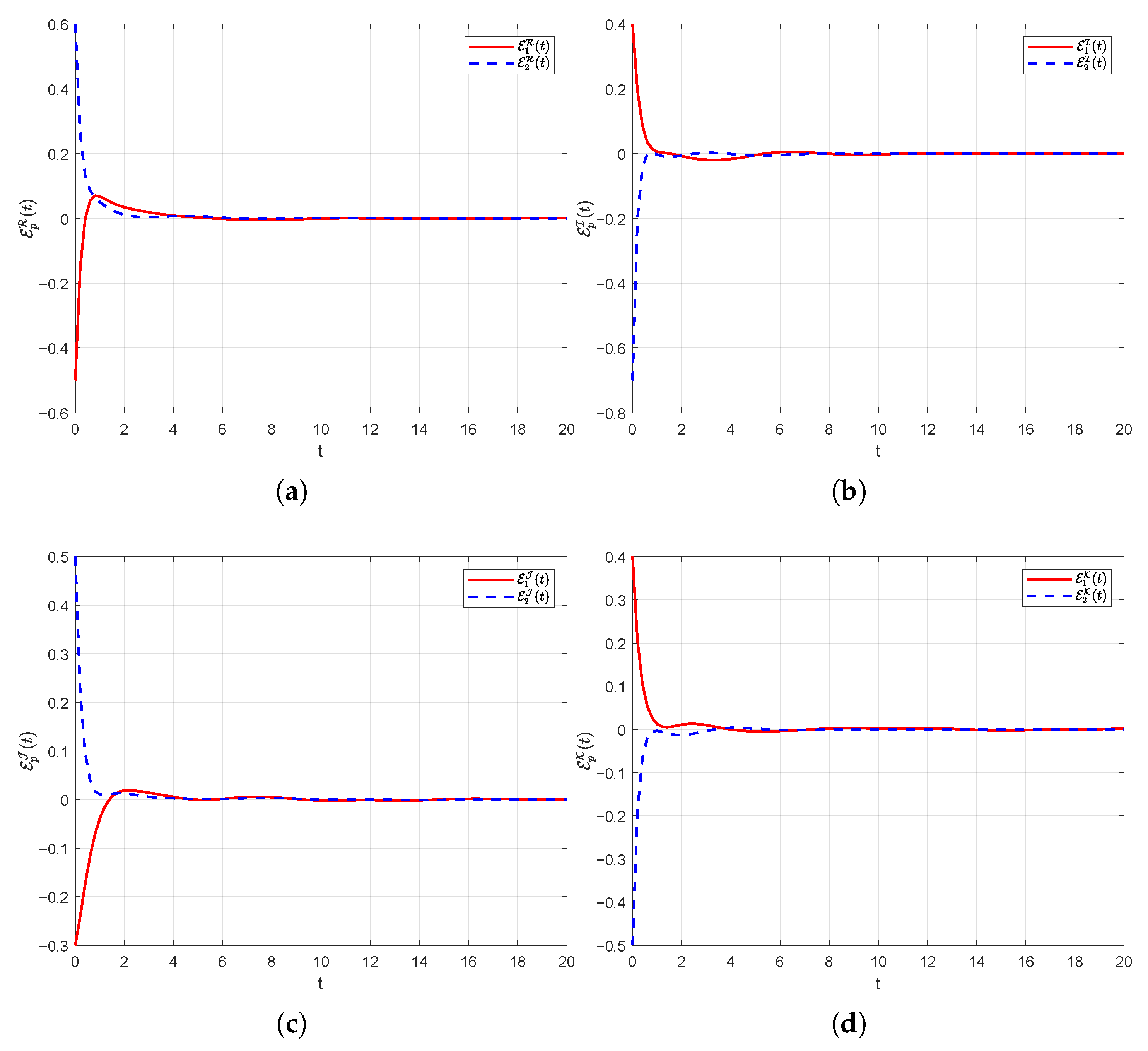
max p = 1 , 2 2 ( θ p + ζ p ) + 2 ξ + q = 1 ϑ ( α p q 2 + β p q 2 ) + n ( L q f ) 2 + n ( L q g ) 2 = 0.4413 < 0 .
The condition of Theorem 1 is thus satisfied, confirming that synchronization is achieved between the drive and response systems. The corresponding synchronization results are illustrated in Figure 4.
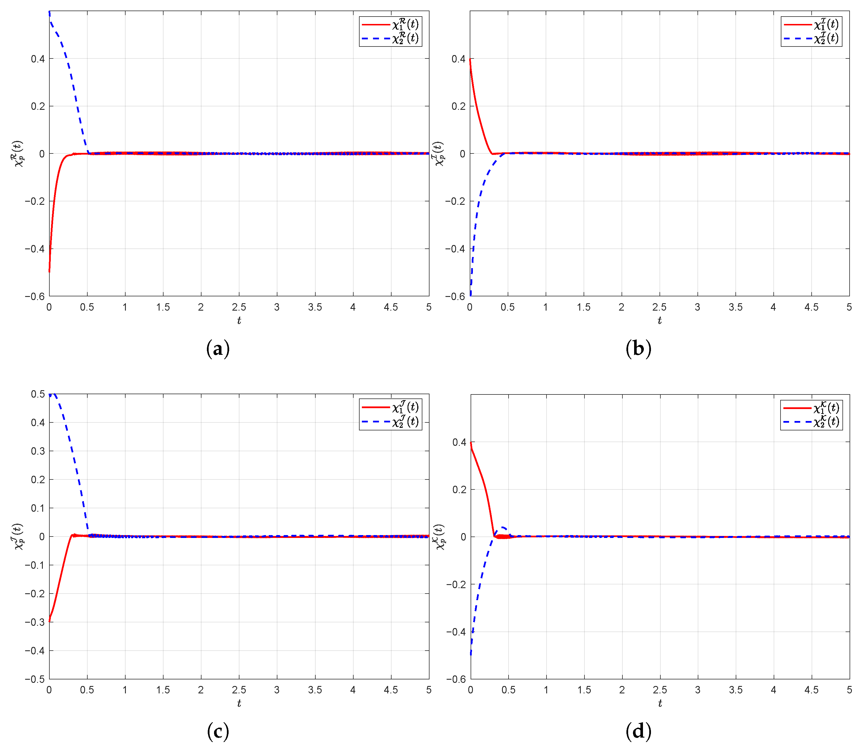
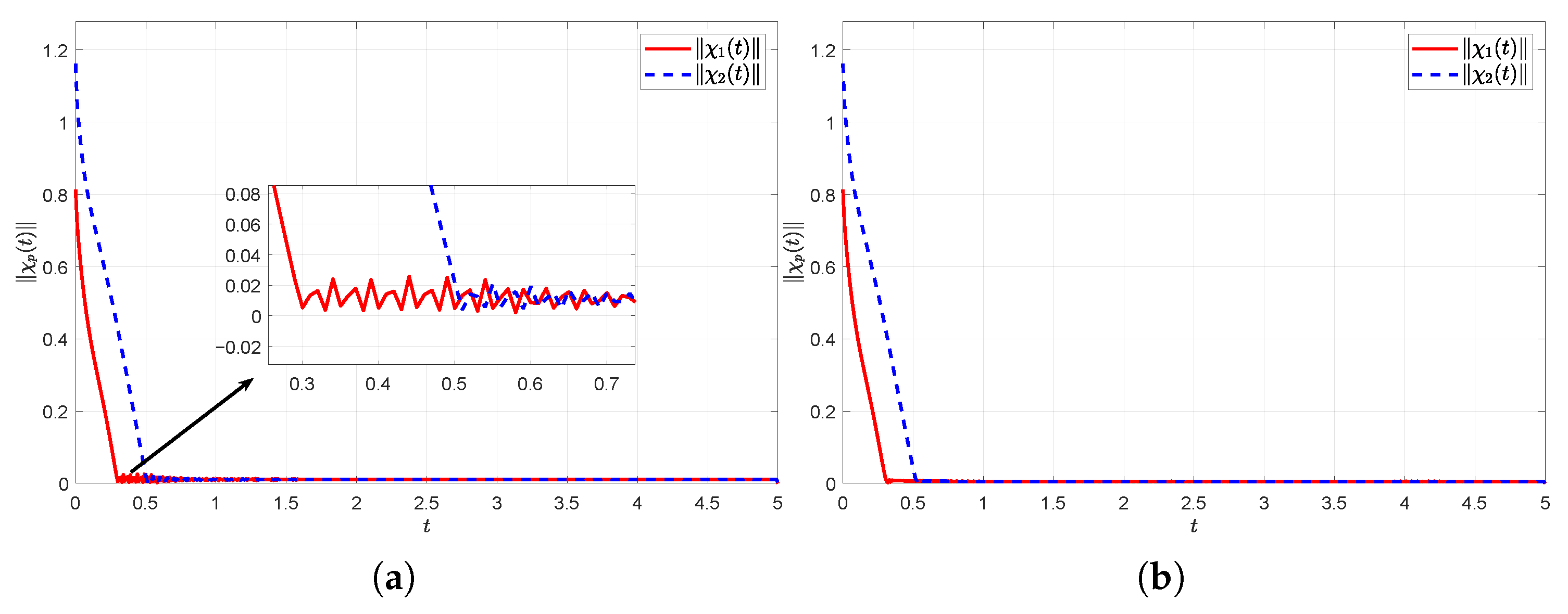
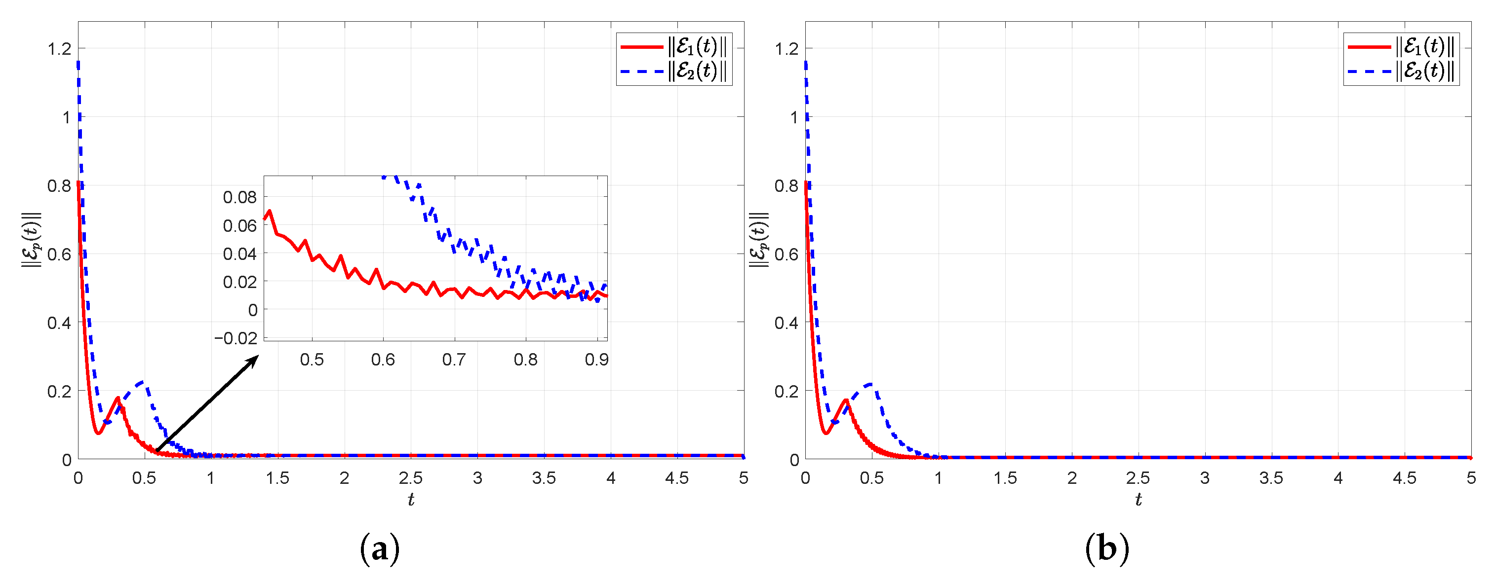
The conditions of Theorem 2 are satisfied with μ 1 = μ 2 = 2 . Consequently, under the control input (13), the sliding surface (6) is reached within a finite time, thus driving the error system states to the manifold χ p = 0 . This finite-time convergence is numerically verified in Figure 5, Figure 6 and Figure 7. In particular, Figure 5 confirms the reachability of the sliding surface, while Figure 6 and Figure 7 depict the norms of the system error and the sliding surface, respectively, converging to zero within the specified finite time.
Remark 8.
The sign function in control law (13) may lead to chattering phenomena, which can be handled in practical implementations via smooth continuous approximations. Common engineering strategies include the boundary layer method [48] and smooth function substitution [39]. In this paper, the smooth function χ p ( t ) ς + χ p ( t ) is adopted to approximate χ p ( t ) , where ς is a small positive design parameter. Smaller ς better approximates ideal SMC law but retains more chattering; larger ς yields smoother control but sacrifices accuracy and convergence speed. To balance both, this paper sets ς = 0.005 . As can be observed from Figure 6 and Figure 7, this approach effectively reduces chattering.
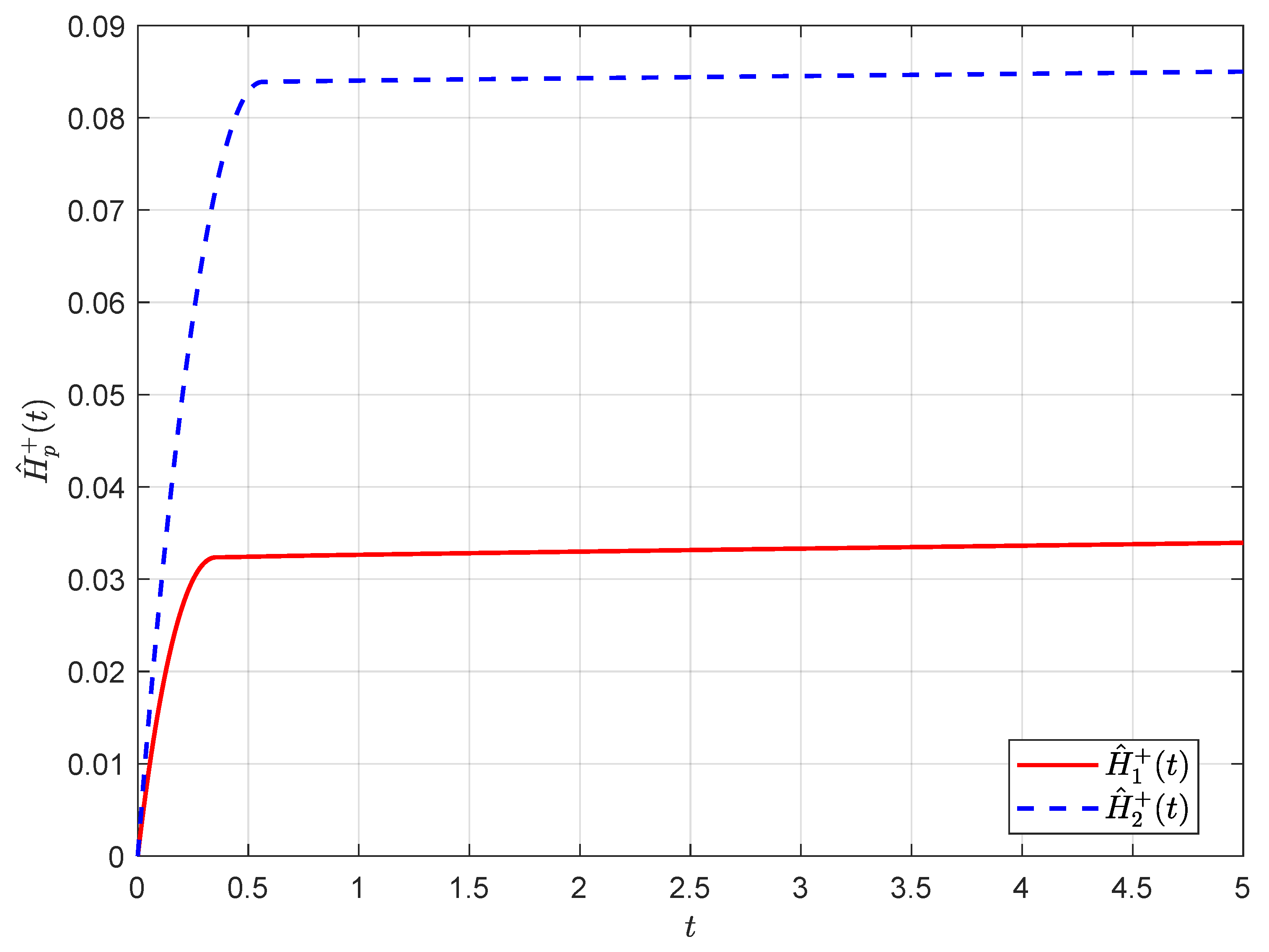
When the upper bound H p + is unknown, the assignment μ ˜ 1 = μ ˜ 2 = 2 is applied according to Theorem 3. The resulting transients of the adaptive laws H ˜ p + ( t ) are presented in Figure 8.
Example 2.
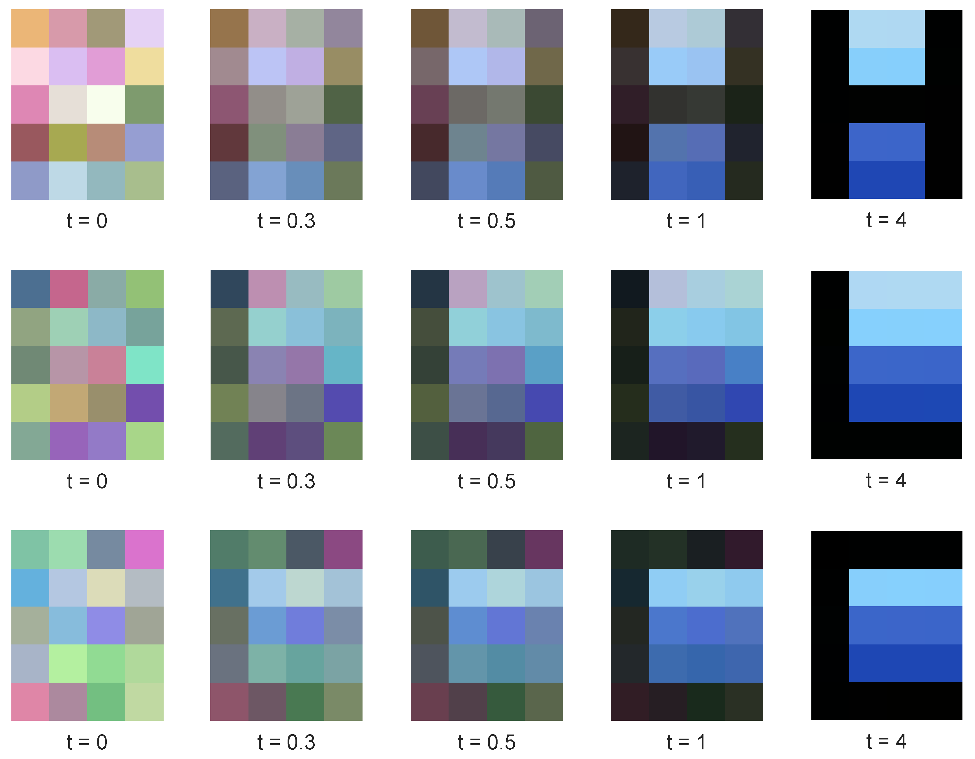
For the “H”, “L”, and “C” color patterns presented in Figure 9, QVNNs structured as in (1) are applied for image storage and retrieval.
As shown in Figure 9, each image has a resolution of 5 × 4 pixels. Thus, we construct QVNNs with a 20-D EP, comprising 20 neurons to store the pattern’s color information.
QVNNs (1) with parameters are set as: θ p = 1.5 ,
α p q = 0.3 + 0.22 i 1.2 j + 0.6 k , p < q 0.5 + 0.2 i + 0.2 j + 0.5 k , p = q 0.5 0.31 i + 0.3 j + 0.42 k , p > q
β p q = 0.3 + 0.41 i + 0.1 j + 0.4 k , p < q 0.1 0.71 i + 0.5 j 0.41 k , p = q 0.6 0.2 i + 0.3 j + 0 k , p > q
Δ α p q ( t ) = 0.4 cos ( t ) + 0.4 sin ( t ) i 0.6 sin ( t ) j 0.4 sin ( t ) k , p < q 0.4 sin ( t ) 0.6 cos ( t ) i 0.4 cos ( t ) j + 0.4 sin ( t ) k , p = q 0.4 cos ( t ) 0.4 cos ( t ) i + 0.4 sin ( t ) j + 0.6 cos ( t ) k , p > q
Δ β p q ( t ) = 0.6 cos ( t ) 0.4 cos ( t ) i + 0.4 cos ( t ) j + 0.4 sin ( t ) k , p < q 0.4 cos ( t ) + 0.6 cos ( t ) i + 0.4 sin ( t ) j 0.4 cos ( t ) k , p = q 0.4 sin ( t ) 0.4 cos ( t ) i + 0.4 sin ( t ) j 0.6 sin ( t ) k , p > q
where p , q = 1 , 2 , 20 . The activation functions are identical to those in Example 1.
Digital color images are characterized by color models that establish a standardized system for interpreting color information. This study utilizes the widely adopted R G B (Red, Green, Blue) framework. Within this system, all colors are synthesized by adjusting the intensity levels of its three primary color channels. Each channel’s intensity is encoded as an integer value (gray level) spanning from 0 (minimum) to 255 (maximum). To enable integrated processing of color data, we implement a quaternion-based approach. According to [49], there exists a bijection from the R G B components ( r , g , b ) to pure imaginary quaternions, defined by r i + g j + b k . This mapping maintains color integrity while offering mathematical convenience for computation.
The EPs are essential for the QVNNs to store and recall the “H”, “L”, and “C” color images. Those given in Table 1 serve as stable memory states, enabling accurate pattern retrieval under appropriate external input.
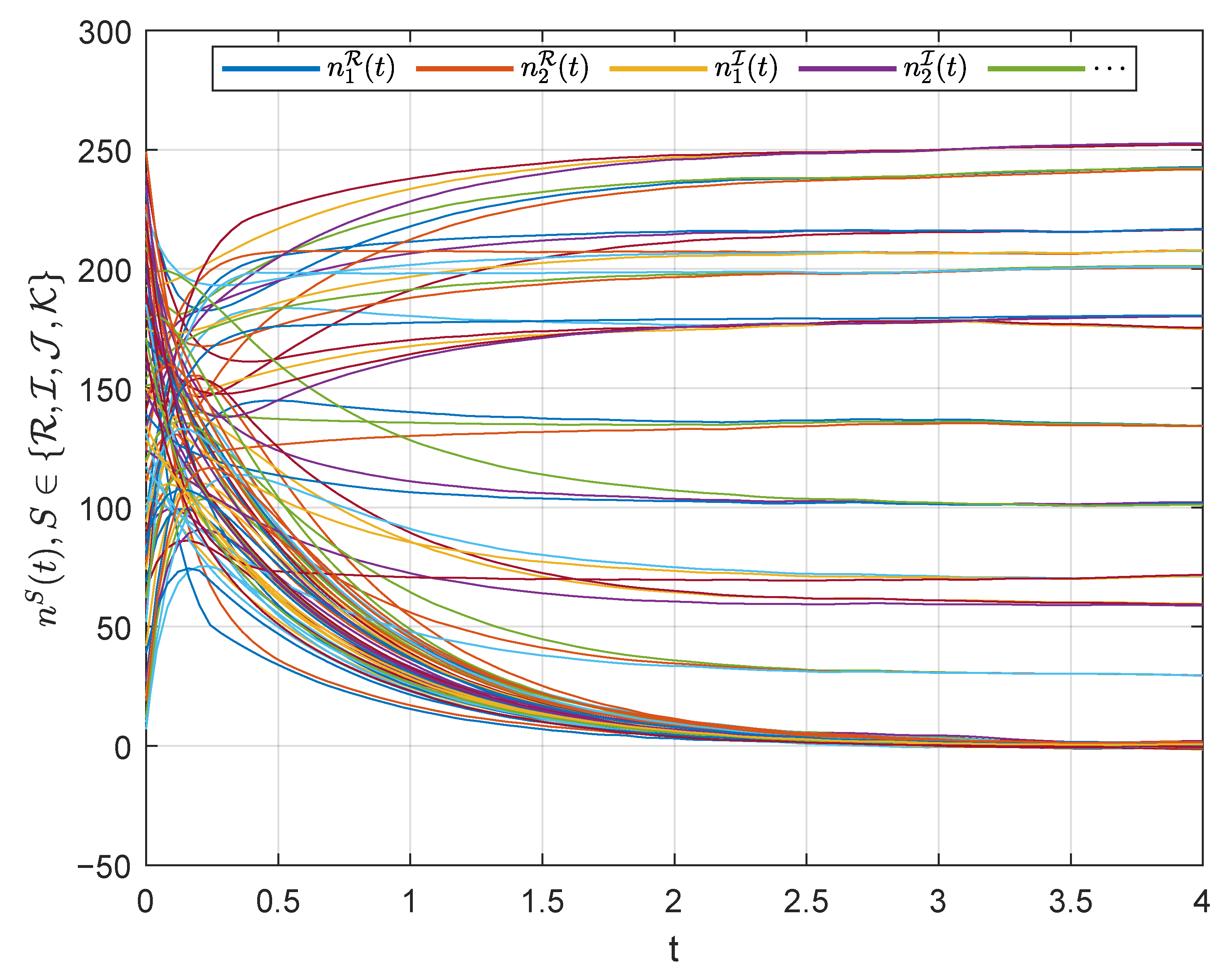
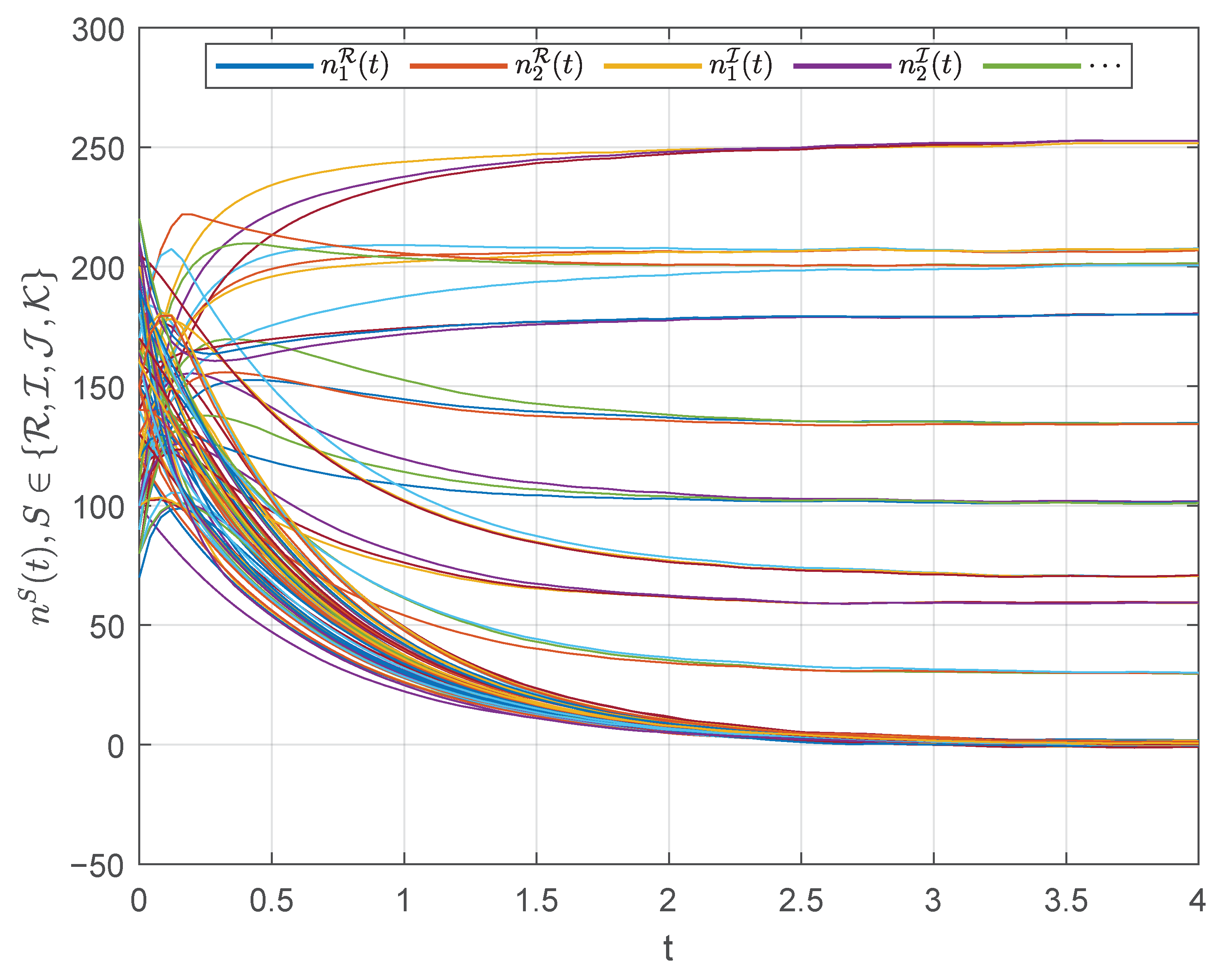
Using the EPs listed in Table 1, the external input quaternion vector is constructed as J ( t ) = [ J 1 ( t ) , J 2 ( t ) , . . . , J 20 ( t ) ] T Q 20 . The ability of the designed network to retrieve the patterns “H”, “L”, and “C” is displayed in Figure 10, beginning from the random initial states m ^ ( 0 ) = [ m ^ 1 ( 0 ) , m ^ 2 ( 0 ) , . . . , m ^ 20 ( 0 ) ] T . The figure displays the evolution of the retrieved patterns at distinct time instances: t = 0 , t = 0.3 , t = 0.5 , t = 1 , and t = 4 .
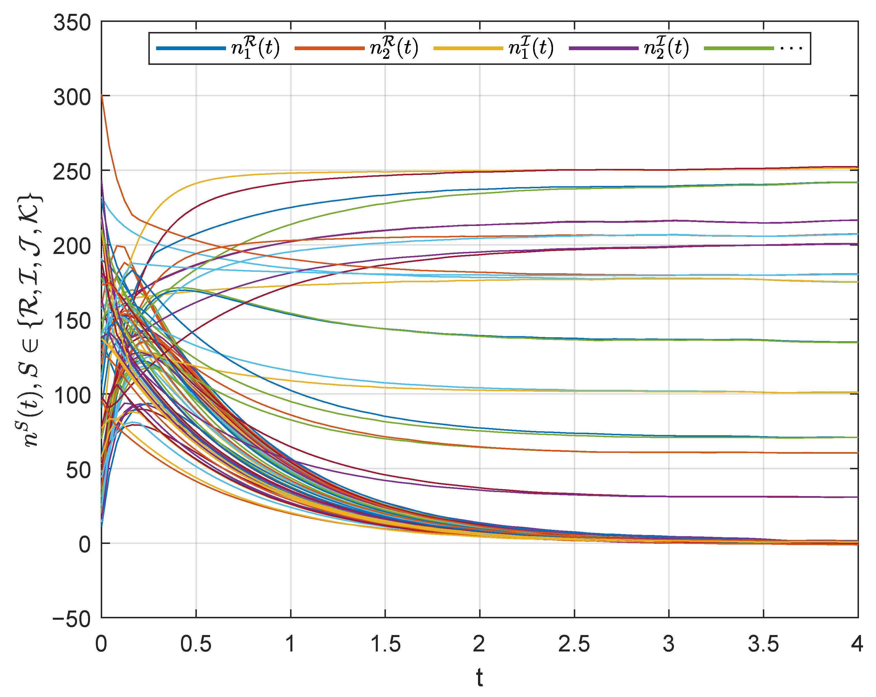
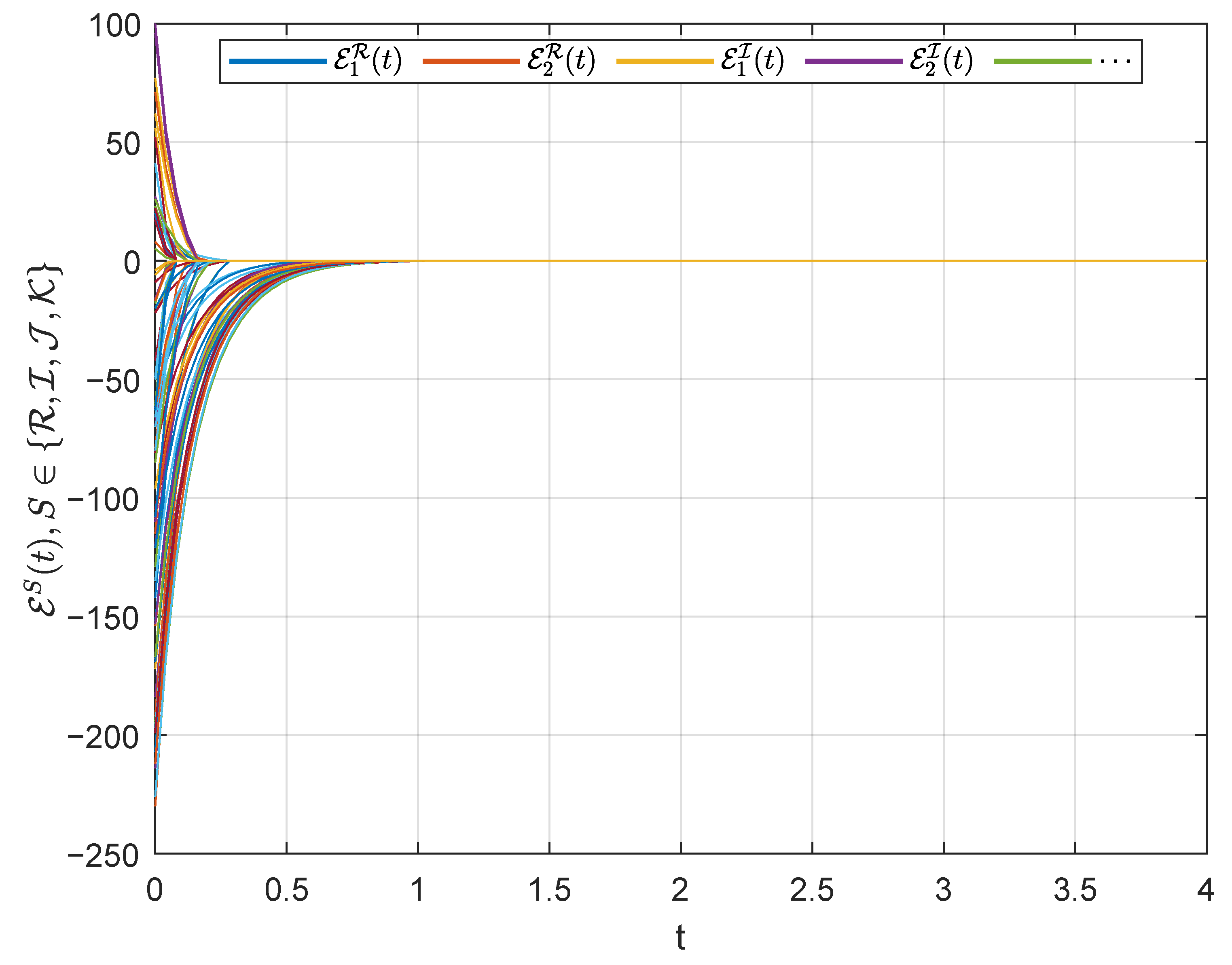
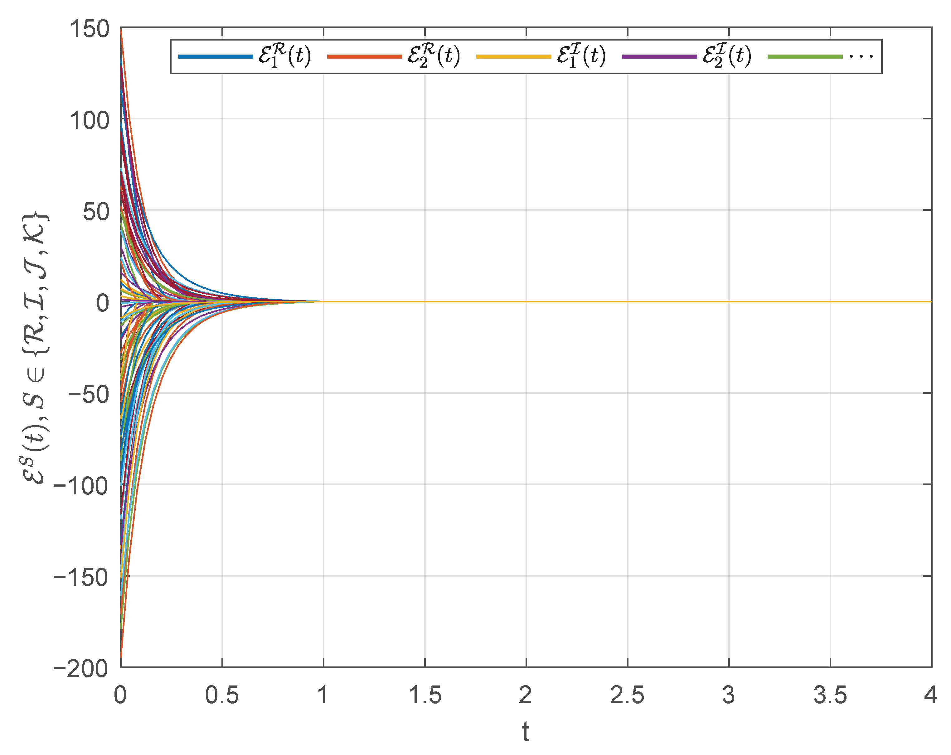
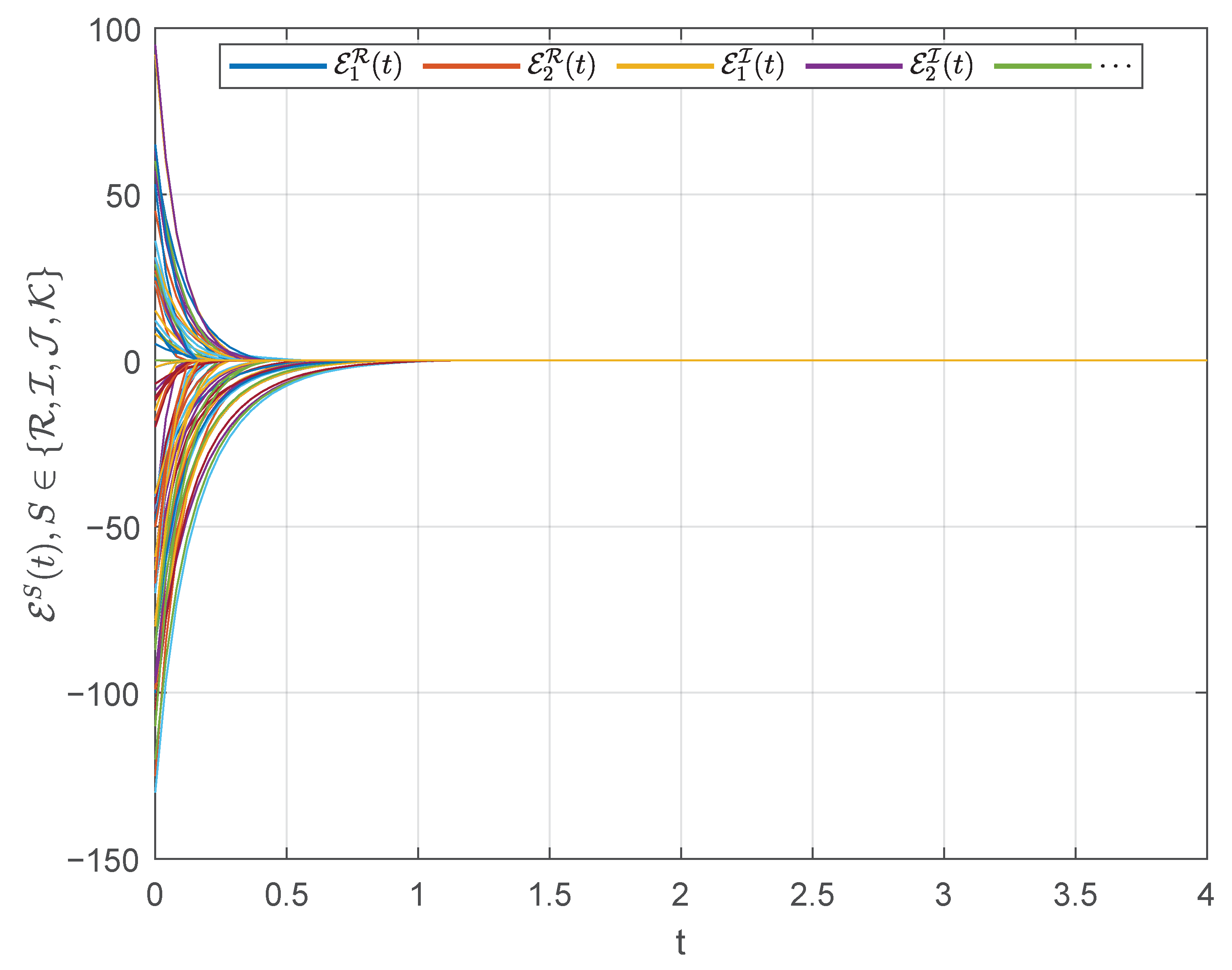
The initial state of the network at t = 0 is characterized by random values, yielding patterns that are not yet clearly identifiable, a result presented in Figure 10. Over time, the images progressively take form, increasingly resembling the target patterns. By t = 0.5 , recognizable structural traits of the letters “H”, “L”, and “C” start to emerge, highlighting the network’s capacity to enhance recall accuracy. Ultimately, at t = 4 , the restored images match the initial images exactly, verifying the effective performance of the implemented QVNNs. Such progressive improvement demonstrates the presented network’s robust synchronization capacity for precisely storing and reconstructing color image patterns. As shown in Figure 11, Figure 12, Figure 13, Figure 14, Figure 15 and Figure 16, the dynamic reconstruction process of the images “H”, “L”, and “C” can be synchronized.
Remark 9.
Whereas RVNNs encode the RGB channels of a pixel across three neurons, QVNNs compactly represent them in a single neuron via pure quaternion components. As Example 2 illustrates, a 5 × 4 color image thus requires only 20 neurons in a QVNN, compared to 60 in a real-valued network for similar performance.

5. Conclusions

This paper investigates the polynomial sliding mode synchronization control for QVNNs subject to proportional delays, parameter uncertainties, and external disturbances. The infinity norm is selected as the norm for quaternion vectors to simplify the derivation process. First, an appropriate integral sliding mode surface is constructed for the system, and the corresponding equivalent controller is derived. Then, owing to quaternion non-commutativity, a non-decomposition strategy is adopted. By constructing a delay-free Lyapunov functional and utilizing certain properties of quaternions, sufficient delay-independent criteria for synchronization are derived. Subsequently, a SMC law is devised, with reachability analysis conducted for the sliding mode surface. For cases where the upper bound of external disturbance is unknown, an adaptive SMC law is further developed. Finally, the effectiveness of the conclusions is comprehensively verified through a two-dimensional numerical example, and the research results are applied to color image pattern storage and retrieval. The impulse phenomenon is regarded as an intrinsic characteristic that cannot be overlooked in both natural and artificial NNs. Therefore, designing effective control synthesis methods for quaternion-valued models with such characteristics will become a critical and urgent research topic.

Author Contributions

Conceptualization, L.Q.; methodology, L.Q. and L.W.; software, Z.J. All authors have read and agreed to the published version of the manuscript.

Funding

This research received no external funding.

Data Availability Statement

The original contributions presented in this study are included in the article. Further inquiries can be directed to the corresponding author.

Conflicts of Interest

The authors declare no conflicts of interest.

References

  1. Zeng, Z.; Wang, J. Associative memories based on continuous-time cellular neural networks designed using space-invariant cloning templates. Neural Netw. 2009, 22, 651–657. [Google Scholar] [CrossRef]
  2. Bao, G.; Wen, S.; Zeng, Z. Robust stability analysis of interval fuzzy Cohen-Grossberg neural networks with piecewise constant argument of generalized type. Neural Netw. 2012, 33, 32–41. [Google Scholar] [CrossRef]
  3. Taluja, A.; Kumar, H.; Thangarasu, J.; Pingle, Y.P. A blockchain-enabled quaternion evolutionary gravitational neocognitron neural network for securing IoT healthcare data in cloud environment. Evol. Syst. 2025, 16, 90. [Google Scholar] [CrossRef]
  4. Suganthi, P.; Kavitha, R. Secure and privacy in healthcare data using quaternion based neural network and encoder-elliptic curve deep neural network with blockchain on the cloud environment. Sādhanā 2023, 48, 206. [Google Scholar] [CrossRef]
  5. Fernández-Torras, A.; Comajuncosa-Creus, A.; Duran-Frigola, M.; Aloy, P. Connecting chemistry and biology through molecular descriptors. Curr. Opin. Chem. Biol. 2022, 66, 102090. [Google Scholar] [CrossRef]
  6. Zhou, L.; Zhao, Z. Exponential synchronization and polynomial synchronization of recurrent neural networks with and without proportional delays. Neurocomputing 2020, 372, 109–116. [Google Scholar] [CrossRef]
  7. Cheng, L.; Tang, F.; Shi, X.; Chen, X.; Qiu, J. Finite-time and fixed-time synchronization of delayed memristive neural networks via adaptive aperiodically intermittent adjustment strategy. IEEE Trans. Neural Netw. Learn. Syst. 2022, 34, 8516–8530. [Google Scholar] [CrossRef] [PubMed]
  8. Gong, S.; Guo, Z.; Wen, S. Finite-time synchronization of T-S fuzzy memristive neural networks with time delay. Fuzzy Sets Syst. 2023, 459, 67–81. [Google Scholar] [CrossRef]
  9. Sheng, Y.; Huang, T.; Zeng, Z. Exponential stabilization of fuzzy memristive neural networks with multiple time delays via intermittent control. IEEE Trans. Syst. Man Cybern. Syst. 2022, 52, 3092–3101. [Google Scholar] [CrossRef]
  10. Zhou, L.; Han, J.; Yang, X. Adaptive synchronization of memristive complex-Valued neural networks with proportional delays and its application to image encryption. Nonlinear Dyn. 2025, 113, 35255–35271. [Google Scholar] [CrossRef]
  11. Zhang, J.; Li, Z.; Cao, J.; Meng, X. Global polynomial synchronization of quaternion-valued inertial neural networks with proportional delay and mismatched parameters. Math. Methods Appl. Sci. 2025, 48, 11113–11123. [Google Scholar] [CrossRef]
  12. Zhang, Y.; Zhou, L. Novel global polynomial stability criteria of impulsive complex-valued neural networks with multi-proportional delays. Neural Comput. Appl. 2022, 34, 2913–2924. [Google Scholar] [CrossRef]
  13. Wang, W.; Wang, J. Convex combination of two geometric-algebra least mean square algorithms and its performance analysis. Signal Process. 2022, 192, 108333. [Google Scholar] [CrossRef]
  14. Cheng, Y.; Shi, Y. The exponential synchronization and asymptotic synchronization of quaternion-valued memristor-based Cohen-Grossberg neural networks with time-varying delays. Neural Process. Lett. 2023, 55, 6637–6656. [Google Scholar] [CrossRef]
  15. Ke, Y.; Ma, C.; Jia, Z.; Xie, Y.; Liao, R. Quasi non-negative quaternion matrix factorization with application to color face recognition. J. Sci. Comput. 2023, 95, 38. [Google Scholar] [CrossRef]
  16. Zhao, N.; Qiao, Y.; Xu, C. New results on synchronization control of memristor-based quaternion-valued fuzzy neural networks with delayed impulses. Fuzzy Sets Syst. 2024, 484, 108940. [Google Scholar] [CrossRef]
  17. Baluni, S.; Yadav, V.K.; Das, S. Quasi-projective synchronization of non-identical time-varying delayed quaternion-valued neural networks with interaction terms: Direct method. Eng. Appl. Artif. Intell. 2024, 136, 108866. [Google Scholar] [CrossRef]
  18. Kandasamy, U.; Li, X.; Rajan, R. Quasi-synchronization and bifurcation results on fractional-order quaternion-valued neural networks. IEEE Trans. Neural Netw. Learn. Syst. 2020, 31, 4063–4072. [Google Scholar] [CrossRef]
  19. Li, R.; Cao, J.; Li, N. Quasi-synchronization control of quaternion-valued fuzzy memristive neural networks. Fuzzy Sets Syst. 2023, 472, 108701. [Google Scholar] [CrossRef]
  20. Huang, Q.; Yu, Y.; Cao, J. Projective synchronization of inertial quaternion-valued neural networks via non-reduced order approach. Neural Process. Lett. 2024, 56, 21. [Google Scholar] [CrossRef]
  21. Zhao, H.; Zhou, L.; Liu, A.; Niu, S.; Gao, X.; Zong, X.; Li, X.; Li, L. A novel predefined-time projective synchronization strategy for multi-modal memristive neural networks. Cogn. Neurodyn. 2025, 19, 50. [Google Scholar] [CrossRef]
  22. Xiong, K.; Hu, C.; Yu, J. Direct approach-based synchronization of fully quaternion-valued neural networks with inertial term and time-varying delay. Chaos Solitons Fractals 2023, 172, 113556. [Google Scholar] [CrossRef]
  23. Zhang, J.; Li, Z.; Cao, J.; Abdel-Aty, M.; Meng, X. Polynomial synchronization of quaternion-valued fuzzy cellular neural networks with proportional delays. Nonlinear Dyn. 2025, 113, 3523–3542. [Google Scholar] [CrossRef]
  24. Liu, Y.; Zhang, D.; Lu, J.; Cao, J. Global μ-stability criteria for quaternion-valued neural networks with unbounded time-varying delays. Inf. Sci. 2016, 360, 273–288. [Google Scholar] [CrossRef]
  25. Chen, X.; Li, Z.; Song, Q.; Hu, J.; Tan, Y. Robust stability analysis of quaternion-valued neural networks with time delays and parameter uncertainties. Neural Netw. 2017, 91, 55–65. [Google Scholar] [CrossRef]
  26. Cheng, Y.; Shi, Y.; Guo, J. Exponential synchronization of quaternion-valued memristor-based Cohen-Grossberg neural networks with time-varying delays: Norm method. Cogn. Neurodyn. 2024, 18, 1943–1953. [Google Scholar] [CrossRef] [PubMed]
  27. Singh, S.; Das, S.; Chouhan, S.; Cao, J. Anti-synchronization of inertial neural networks with quaternion-valued and unbounded delays: Non-reduction and non-separation approach. Knowl.-Based Syst. 2023, 278, 110903. [Google Scholar] [CrossRef]
  28. Zhang, H.; Zeng, Z.; Han, Q. Synchronization of multiple reaction–diffusion neural networks with heterogeneous and unbounded time-varying delays. IEEE Trans. Cybern. 2019, 49, 2980–2991. [Google Scholar] [CrossRef]
  29. Sheng, Y.; Zhang, H.; Zeng, Z. Stability and robust stability of stochastic reaction–diffusion neural networks with infinite discrete and distributed delays. IEEE Trans. Syst. Man Cybern. Syst. 2020, 50, 1721–1732. [Google Scholar] [CrossRef]
  30. Zhou, L. On the global dissipativity of a class of cellular neural networks with multipantograph delays. Adv. Artif. Neural Syst. 2011, 2011, 941426. [Google Scholar] [CrossRef]
  31. Assali, E.A. Direct approach on projective synchronization of inertial quaternion-valued neural networks with proportional delays. Comput. Appl. Math. 2024, 43, 441. [Google Scholar] [CrossRef]
  32. Liang, X.; Wang, H.; Zhang, Y. Adaptive nonsingular terminal sliding mode control for rehabilitation robots. Comput. Electr. Eng. 2022, 99, 107718. [Google Scholar] [CrossRef]
  33. Jiang, W.; Ge, S.S.; Li, D. Fixed-time-synchronized control: A system-dimension-categorized approach. Sci. China Inf. Sci. 2023, 66, 172203. [Google Scholar] [CrossRef]
  34. Wan, Y.; Zhou, L.; Han, J. Global polynomial synchronization of proportional delay memristive neural networks with uncertain parameters and its application to image encryption. Eng. Appl. Artif. Intell. 2025, 147, 110290. [Google Scholar] [CrossRef]
  35. Guo, R.; Xu, S.; Guo, J. Sliding-mode synchronization control of complex-valued inertial neural networks with leakage delay and time-varying delays. IEEE Trans. Syst. Man Cybern. Syst. 2023, 53, 1095–1103. [Google Scholar] [CrossRef]
  36. Wang, L.; Song, Q.; Zhao, Z.; Liu, Y.; Alsaadi, F.E. Synchronization of two nonidentical complex-valued neural networks with leakage delay and time-varying delays. Neurocomputing 2019, 356, 52–59. [Google Scholar] [CrossRef]
  37. Zhang, H.; Wang, X.; Lin, X. Synchronization of complex-valued neural network with sliding mode control. J. Frankl. Inst. 2016, 353, 345–358. [Google Scholar] [CrossRef]
  38. Aouiti, C.; Bessifi, M. Sliding mode control for finite-time and fixed-time synchronization of delayed complex-valued recurrent neural networks with discontinuous activation functions and nonidentical parameters. Eur. J. Control 2021, 59, 109–122. [Google Scholar] [CrossRef]
  39. Guo, R.; Xu, S.; Ahn, C.K. Dissipative sliding-mode synchronization control of uncertain complex-valued inertial neural networks: Non-reduced-order strategy. IEEE Trans. Circuits Syst. I Regul. Pap. 2023, 70, 860–871. [Google Scholar] [CrossRef]
  40. Bi, C.; Li, Z.; Cao, J.; Meng, X.; Karamti, H. Sliding mode synchronization control of delayed quaternion-valued neural networks and its application. J. Frankl. Inst. 2025, 362, 107926. [Google Scholar] [CrossRef]
  41. Huang, Y.; Li, A. General decay anti-synchronization of coupled delayed memristive neural networks with constant and time-varying distributed-delay coupling. Neurocomputing 2025, 618, 129058. [Google Scholar] [CrossRef]
  42. Zhang, X.; Li, C.; Li, H.; Xu, J. Synchronization of neural networks involving distributed-delay coupling: A distributed-delay differential inequalities approach. IEEE Trans. Neural Netw. Learn. Syst. 2024, 35, 8086–8096. [Google Scholar] [CrossRef]
  43. Li, L.; Chen, W.; Wu, X. Global exponential stability and synchronization for novel complex-valued neural networks with proportional delays and inhibitory factors. IEEE Trans. Cybern. 2021, 51, 2142–2152. [Google Scholar] [CrossRef] [PubMed]
  44. Zhou, L.; Zhu, Q.; Huang, T. Global polynomial synchronization of proportional delayed inertial neural networks. IEEE Trans. Syst. Man Cybern. Syst. 2023, 53, 4487–4497. [Google Scholar] [CrossRef]
  45. Peng, T.; Qiu, J.; Lu, J.; Tu, Z.; Cao, J. Finite-time and fixed-time synchronization of quaternion-valued neural networks with/without mixed delays: An improved one-norm method. IEEE Trans. Neural Netw. Learn. Syst. 2022, 33, 7475–7487. [Google Scholar] [CrossRef] [PubMed]
  46. Shang, W.; Zhang, W.; Chen, D.; Cao, J. New criteria of finite time synchronization of fractional-order quaternion-valued neural networks with time delay. Appl. Math. Comput. 2023, 436, 127484. [Google Scholar] [CrossRef]
  47. Sun, X.; Song, X.; Man, J.; Wu, N. Quasi-synchronization for fractional-order reaction–diffusion quaternion-valued neural networks: An LMI approach. Neural Process. Lett. 2023, 55, 4499–4517. [Google Scholar] [CrossRef]
  48. Zheng, W.; Qu, S.; Tang, Q. Sliding mode synchronization of uncertain memristor cellular neural network and application in secure communication. Neural Comput. Appl. 2024, 36, 7845–7859. [Google Scholar] [CrossRef]
  49. Chen, X.; Song, Q.; Li, Z. Design and analysis of quaternion-valued neural networks for associative memories. IEEE Trans. Syst. Man Cybern. Syst. 2018, 48, 2305–2314. [Google Scholar] [CrossRef]
Figure 1. Chaotic behavior of first neuron. (a) Trajectories of the chaotic attractor for n 1 R ( t ) , n 1 I ( t ) , and n 1 J ( t ) . (b) Trajectories of the chaotic attractor for n 1 R ( t ) , n 1 I ( t ) , and n 1 K ( t ) . (c) Trajectories of the chaotic attractor for n 1 R ( t ) , n 1 J ( t ) , and n 1 K ( t ) . (d) Trajectories of the chaotic attractor for n 1 I ( t ) , n 1 J ( t ) , and n 1 K ( t ) .
Axioms 15 00072 g001aAxioms 15 00072 g001b
Figure 2. Chaotic behavior of second neuron. (a) Trajectories of the chaotic attractor for n 2 R ( t ) , n 2 I ( t ) , and n 2 J ( t ) . (b) Trajectories of the chaotic attractor for n 2 R ( t ) , n 2 I ( t ) , and n 2 K ( t ) . (c) Trajectories of the chaotic attractor for n 2 R ( t ) , n 2 J ( t ) , and n 2 K ( t ) . (d) Trajectories of the chaotic attractor for n 2 I ( t ) , n 2 J ( t ) , and n 2 K ( t ) .
Axioms 15 00072 g002
Figure 3. Phase trajectories of the error system without controller for p = 1 , 2 . (a) Phase trajectories of the E p R . (b) Phase trajectories of the E p I . (c) Phase trajectories of the E p J . (d) Phase trajectories of the E p K .
Axioms 15 00072 g003
Figure 4. Phase trajectories of the error system under controller (8) for p = 1 , 2 . (a) Phase trajectories of the E p R . (b) Phase trajectories of the E p I . (c) Phase trajectories of the E p J . (d) Phase trajectories of the E p K .
Axioms 15 00072 g004
Figure 5. Phase trajectories of the sliding-mode surface in (6) under controller (13) for p = 1 , 2 . (a) Phase trajectories of the χ p R . (b) Phase trajectories of the χ p I . (c) Phase trajectories of the χ p J . (d) Phase trajectories of the χ p K .
Axioms 15 00072 g005
Figure 6. Norm of the sliding surface χ p ( t ) for p = 1 , 2 . (a) Without the smooth approximation. (b) With the smooth approximation.
Axioms 15 00072 g006
Figure 7. Evolution of the synchronization error norm E p ( t ) between (26) and (27) under the SMC law (13) for p = 1 , 2 . (a) Without the smooth approximation. (b) With the smooth approximation.
Axioms 15 00072 g007
Figure 8. Adaptive law of H ^ p + ( t ) , where p = 1 , 2 .
Axioms 15 00072 g008
Figure 9. Original color images of patterns “H”, “L”, and “C”.
Axioms 15 00072 g009
Figure 10. Simulation of retrieving the patterns “H”, “L”, and “C” at time t = 0, 0.3, 0.5, 1 and 4 with the different initial value.
Axioms 15 00072 g010
Figure 11. Trajectories of the response system for the image pattern “H”.
Axioms 15 00072 g011
Figure 12. Trajectories of the synchronization errors for the image pattern “H”.
Axioms 15 00072 g012
Figure 13. Trajectories of the response system for the image pattern “L”.
Axioms 15 00072 g013
Figure 14. Trajectories of the synchronization errors for the image pattern “L”.
Axioms 15 00072 g014
Figure 15. Trajectories of the response system for the image pattern “C”.
Axioms 15 00072 g015
Figure 16. Trajectories of the error system for the image pattern “C”.
Axioms 15 00072 g016
Table 1. EPs selected for the “H”, “L”, and “C” color images.
EPColor Image “H”Color Image “L”Color Image “C”
m ¯ 1 0 ( 0 + 0 i + 0 j + 0 k ) 00
m ¯ 2 176 i + 216 j + 242 k 176 i + 216 j + 242 k 0
m ¯ 3 176 i + 216 j + 242 k 176 i + 216 j + 242 k 0
m ¯ 4 0 176 i + 216 j + 242 k 0
m ¯ 5 000
m ¯ 6 135 i + 206 j + 251 k 135 i + 206 j + 251 k 135 i + 206 j + 251 k
m ¯ 7 135 i + 206 j + 251 k 135 i + 206 j + 251 k 135 i + 206 j + 251 k
m ¯ 8 0 135 i + 206 j + 251 k 135 i + 206 j + 251 k
m ¯ 9 000
m ¯ 10 0 60 i + 100 j + 200 k 60 i + 100 j + 200 k
m ¯ 11 0 60 i + 100 j + 200 k 60 i + 100 j + 200 k
m ¯ 12 0 60 i + 100 j + 200 k 60 i + 100 j + 200 k
m ¯ 13 000
m ¯ 14 60 i + 100 j + 200 k 30 i + 70 j + 180 k 30 i + 70 j + 180 k
m ¯ 15 60 i + 100 j + 200 k 30 i + 70 j + 180 k 30 i + 70 j + 180 k
m ¯ 16 0 30 i + 70 j + 180 k 30 i + 70 j + 180 k
m ¯ 17 000
m ¯ 18 30 i + 70 j + 180 k 00
m ¯ 19 30 i + 70 j + 180 k 00
m ¯ 20 000
Disclaimer/Publisher’s Note: The statements, opinions and data contained in all publications are solely those of the individual author(s) and contributor(s) and not of MDPI and/or the editor(s). MDPI and/or the editor(s) disclaim responsibility for any injury to people or property resulting from any ideas, methods, instructions or products referred to in the content.