Bifurcation Analysis of a Semilinear Generalized Friction System with Time-Delayed Feedback Control

Abstract

In this paper, we investigate a semilinear parabolic friction system with time-delay feedback control and diffusion. This model more accurately describes the coupled dynamic behavior between vibrations induced by time-delayed control forces and the diffusion-driven evolution of material surface properties in practical friction processes. Through eigenvalue analysis, it is proven that the system’s stability does not vary monotonically with parameters. Instead, as the time delay varies, the system undergoes a finite number of alternating switches between stability and instability, before eventually losing its stability. The established stability criteria and bifurcation formulae can provide a predictive basis for and strategies to avoid the frictional vibration caused by time-delayed feedback in mechanical systems, providing significant guidance for vibration-reducing design and control parameter optimization in equipment such as braking systems and precision machine tools.

1. Introduction

Friction is a critical aspect of many mechanical systems (such as hydraulic systems, high-quality servo mechanisms, and simple aerodynamic systems); therefore, a good friction model is necessary for predicting the limit cycle, analyzing stability, finding controller gain, and simulating. At present, several friction models have been proposed with frictional sliding [1,2,3,4,5,6,7,8,9,10]. In engineering, many dynamical systems can be described by differential equations of state variables with time evolution [11]. Through studying the friction model with time-delayed feedback control, friction compensation technology can help reduce and prevent engineering accidents caused by friction. The research on semilinear parabolic equations with time delay has attracted many scholars [12,13,14,15]. Unlike dynamical systems described by ordinary differential equations, the solution space of a semilinear parabolic dynamical system with delay is infinite dimensional. The delay may result in changes in dynamic properties (such as the system stability and the existence of periodic solutions) and more complex orbital topology.

Originally, time-delayed feedback control was a method used to control chaos in continuous time systems. This method was first proposed by Pyragas in 1992 [16], and its main idea is to stabilize the unstable periodic orbits contained in the chaotic attractor by using delayed feedback control, thereby transforming the system from a disordered motion state to an ordered one. In [17,18,19], Chen’s system with time-delayed feedback control, the electromagnetic bearing system and van der Pol equation are studied respectively. In [20], the resonance of a cantilever column with time-delayed feedback control is studied, and the time delay and feedback parameters that ensure the system’s stability are obtained. In [21,22], via time-delayed feedback control, the van der Pol oscillators are discussed under three conditions: without external force, with external force, and with parameters.

The paper is structured as follows: Section 2 presents the model’s establishment and the existence of equilibrium points. Section 3 analyzes the stability of equilibria and the stability switches, and explains mathematically that the “stability switch” phenomenon originates from characteristic roots crossing the imaginary axis. Section 4 investigates the Hopf bifurcation properties of the friction system, applying the center manifold theorem and normal form theory to reduce the infinite-dimensional system to a finite-dimensional center manifold. Explicit calculation formulae are derived to determine the direction of Hopf bifurcation (subcritical/supercritical) and the stability of bifurcating periodic solutions. Section 5 provides numerical simulations to intuitively demonstrate the stability switching process.

2. Establishment of the Model

A. Saha et al. [23] proposed two different types of friction models, each incorporating two different time-delayed control forces; the local and global stability boundaries for control gain $K_{c_1}\left(K_{c_2}\right)$ with the time delay ${\tau }_1\left({\tau }_2\right)$ are given when all other parameters are fixed, and the critical belt velocity for the two control forces are compared. Moreover, they used belt velocity as the bifurcation parameter and compared the bifurcation diagrams of two different models. However, they did not provide the detailed Hopf bifurcation analysis with the time delay parameter. After dimensionless processing, the following four models are obtained:

$$\begin{array}{cc}\hfill & \left\{\begin{array}{c}\dot{x}\left(t\right)=y\left(t\right)\hfill \\ \dot{y}\left(t\right)=-\left(1+K_{c_1}\right)x\left(t\right)+K_{c_2}x\left(t-{\tau }_1\right)+h_{1}y\left(t\right)+h_2{y}^2\left(t\right)+h_3{y}^3\left(t\right)\hfill \end{array}\right.\hfill \end{array}$$

(1)

$$\begin{array}{cc}\hfill & \left\{\begin{array}{c}\dot{x}\left(t\right)=y\left(t\right)\hfill \\ \dot{y}\left(t\right)=-x\left(t\right)+K_{c_2}x\left(t-{\tau }_2\right)+h_{1}y\left(t\right)+h_2{y}^2\left(t\right)+h_3{y}^3\left(t\right)\hfill \end{array}\right.\hfill \end{array}$$

(2)

$$\begin{array}{cc}\hfill & \left\{\begin{array}{c}\dot{x}\left(t\right)=y\left(t\right)\hfill \\ \dot{y}\left(t\right)=-x\left(t\right)+K_{c_2}x\left(t-{\tau }_2\right)-2\xi y\left(t\right)+\gamma \left(e^{ay\left(t\right)}-1\right)\hfill \end{array}\right.\hfill \end{array}$$

(3)

$$\begin{array}{cc}\hfill & \left\{\begin{array}{c}\dot{x}\left(t\right)=y\left(t\right)\hfill \\ \dot{y}\left(t\right)=-\left(1+K_{c_1}\right)x\left(t\right)+K_{c_2}x\left(t-{\tau }_1\right)-2\xi y\left(t\right)+\gamma \left(e^{ay\left(t\right)}-1\right)\hfill \end{array}\right.\hfill \end{array}$$

(4)

in which ${\tau }_1\left({\tau }_2\right)$ is time delay of control force 1 (control force 2); for the physical meanings of $K_{c_1},K_{c_2},h_1,h_2,h_3,\xi ,\gamma ,a$, see [23]. Equation (4) is the most widely used exponential model with Stribeck velocity in engineering.

The previous friction model with time-delayed feedback control is a lumped parameter ODE model. Its limitations are mainly reflected in the following three aspects:

(1) It ignores the spatial effect and microscopic process, failing to describe the key physical processes that accompany friction and which are spatially inhomogeneous in distribution within the contact surface.

(2) Heat conduction and thermoelastic instability. Frictional heating will form an inhomogeneous temperature field in the contact area, and thermal expansion will alter the contact pressure distribution and thus exerts a reverse effect on the friction force, forming a spatial–thermal coupled feedback loop that may lead to intense vibration.

(3) Spatial evolution of surface topography and stress. Prolonged frictional wear will alter the surface’s micro-geometric topography and introduce a residual stress field, with these changes varying gradually in space.

Introducing diffusion terms into the friction model with time-delayed feedback represents a key leap from an idealized, localized, abstract model to a physically realistic, global, high-fidelity model. It addresses the fundamental shortcomings of the classical model in terms of its physical completeness, long-term predictability, and the practicality of control strategies. It opens a completely new direction for researching spatiotemporal complex dynamics, multi-physics field coupling, and predictive intelligent control in friction systems. Therefore, introducing diffusion terms into the model (usually in the form of PDEs, such as the heat conduction equations and the diffusion equations) is a fundamental improvement.

Based on this, we generalize the four models proposed by A. Saha et al., and abstract the friction into a function of velocity, $f=f\left(v(x,t)\right)$. At the same time, in the process of friction, the friction surface is repeatedly affected by stress and heat, which will lead to diffusion . Diffusion alters the microstructure and properties of the surface layer, and affects the friction and wear process. Therefore, studying the diffusion process in friction holds great practical significance and theoretical value. Under the homogeneous Neumann boundary conditions, introducing the diffusion term into the generalized friction model, we propose a semilinear parabolic friction model with time-delayed feedback control:

$$\left\{\begin{array}{c}{\displaystyle \frac{\partial u(x,t)}{\partial t}}=d_1\Delta u+v(x,t),t>0,\hfill \\ {\displaystyle \frac{\partial v(x,t)}{\partial t}}=d_2\Delta v+K_{1}u(x,t)+K_{2}u(x,t-\tau )+f\left(v(x,t)\right),t>0,\hfill \\ u_x(0,t)=v_x(0,t)=0, u_x(l\pi ,t)=v_x(l\pi ,t)=0,t>0,\hfill \\ u(x,0)=u_0\left(x\right)\ge 0, v(x,0)=v_0\left(x\right)\ge 0,\hfill \end{array}\right.$$

(5)

where $x\in \mathsf{\Omega }=(0,l\pi ), l>0, f\in C^3\left(\mathbb{R}\right)$, and $f\left(0\right)=0$ is satisfied.

Thermal diffusion d1: The rate at which heat generated at the friction interface diffuses into the bulk material. Wear/damage diffusion d2: The spatial redistribution of material properties caused by wear debris migration and changes in surface topography.

Below, we discuss the conditions that ensure system (5) has meaningful equilibrium points. We make the following assumptions:

(H₁)

$K_1+K_2\ne 0$,

(H₂)

$K_1+K_2=0$,

(H₃)

$f^{\prime }\left(0\right)<0$,

(H₄)

$f^{\prime }\left(0\right)>0$.

Theorem 1. 

For system (5), we can draw the following conclusions:

• (1) If $\left({\mathbf{H}}_{\mathbf{1}}\right)$ is satisfied, then the system has a unique trivial equilibrium $P_0=\left(u_0,v_0\right)=(0,0)$;
• (2) If $\left({\mathbf{H}}_{\mathbf{2}}\right)$ is satisfied, then the system has a semi-trivial equilibrium $P_1=(c,0),c\in \mathbb{R}\setminus \left\{0\right\}$.

3. Stability Analysis of the Semilinear Parabolic Friction System

When $\tau =0$, system (5) becomes

$$\left\{\begin{array}{c}{\displaystyle \frac{\partial u(x,t)}{\partial t}}=d_1\Delta u+v(x,t),x\in \mathsf{\Omega }=(0,l\pi ),t>0,\hfill \\ {\displaystyle \frac{\partial v(x,t)}{\partial t}}=d_2\Delta v+(K_1+K_2)u(x,t)+f\left(v(x,t)\right),x\in \mathsf{\Omega }=(0,l\pi ),t>0,\hfill \\ u_x(0,t)=v_x(0,t)=0,u_x(l\pi ,t)=v_x(l\pi ,t)=0,t>0,\hfill \\ u(x,0)=u_0\left(x\right)\ge 0,v(x,0)=v_0\left(x\right)\ge 0,x\in \mathsf{\Omega }=(0,l\pi ).\hfill \end{array}\right.$$

(6)

We define the real-valued Sobolev space

$$X:=\left\{{\left(u,v\right)}^T\left|u,v\in H^2\left(0,l\pi \right),\left(u_x,v_x\right)\right.{|}_{x=0,l\pi }=\left(0,0\right)\right\},$$

where the complexification of X is

$$X_c:=X\oplus iX=\left\{x_1+i{x}_2\left|x_1,x_2\in X\right.\right\}.$$

Let $U=\left(u,v\right)\in H^2\left(0,l\pi \right),D=diag\left(d_1,d_2\right),$ and $F\left(\alpha ,U\right)=\left(f,g\right)$; then, system (6) can be represented abstractly as follows:

$$\dot{U}\left(t\right)=D\Delta U\left(t\right)+F\left(\alpha ,U\right).$$

We use $J\left(F\right)$ to represent Jacobian matrix of F; then, the linearized operator at $\left(\alpha ,0,0\right)$ is as follows:

$$L\left(\alpha \right)=D{\displaystyle \frac{{\partial }^2}{\partial x^2}}+J\left(F\right){|}_{U\equiv 0}=\left(\begin{array}{cc}{a}_{11}+d_1{\displaystyle \frac{{\partial }^2}{\partial x^2}}& a_{12}\\ a_{21}& a_{22}+d_2{\displaystyle \frac{{\partial }^2}{\partial x^2}}\end{array}\right).$$

Using ${\mu }_n={\displaystyle \frac{n^2}{l^2}}\left(n=0,1,2\dots \right)$ as the nth eigenvalue of $-{\phi }_{xx}=\mu \phi ,{\phi }_x{|}_{x=0,l\pi }=0$, we define the linear operator as follows:

$$L_n\left(\alpha \right)=\left(\begin{array}{cc}{a}_{11}-d_1{\mu }_n& a_{12}\\ a_{21}& a_{22}-d_2{\mu }_n\end{array}\right).$$

Its eigenequation is as follows:

$${\lambda }^2+E_n\left(\alpha \right)\lambda +F_n\left(\alpha \right)=0,$$

(7)

in which

$$\begin{array}{cc} & E_n\left(\alpha \right)=-tr\left(L_n\left(\alpha \right)\right)=-\left(a_{11}+a_{22}\right)+\left(d_1+d_2\right){\mu }_n,\hfill \\ & F_n\left(\alpha \right)=\left|L_n\left(\alpha \right)\right|=d_1{d}_2{{\mu }_n}^2-\left(a_{11}{d}_2+a_{22}{d}_1\right){\mu }_n+a_{11}{a}_{22}-a_{12}{a}_{21}.\hfill \end{array}$$

The corresponding Jacobian matrix of system (6) at $P_0=\left(u_0,v_0\right)=(0,0)$ is $\left(\begin{array}{cc}{a}_{11}& a_{12}\\ a_{21}& a_{22}\end{array}\right)$, with $a_{11}=0, a_{12}=1, a_{21}=K_1+K_2,$ and $a_{22}=f^{\prime }\left(0\right).$ Its characteristic roots are as follows:

$${\lambda }_{1,2}^{\left(n\right)}={\displaystyle \frac{-E_n\pm \sqrt{{E_n}^2-4F_n}}{2}},n\in {\mathbb{N}}_0\triangleq \left\{0\right\}\cup \mathbb{N}.$$

Lemma 1.

Suppose $\left({\mathbf{H}}_{\mathbf{1}}\right)$ holds; we can draw the following conclusions:

• (1) If $\left({\mathbf{H}}_{\mathbf{3}}\right)$ is satisfied, and $K_1+K_2<0$, then $E_n>0, F_n>0$, and all the roots of Equation (7) have negative real parts;
• (2) If $\left({\mathbf{H}}_{\mathbf{4}}\right)$ is satisfied, or $K_1+K_2>0$, then $E_0<0$, and Equation (7) has at least one root with positive real part.

Theorem 2.

Suppose $\left({\mathbf{H}}_{\mathbf{1}}\right)$ holds; the conclusions can be drawn as follows:

• (1) If $\left({\mathbf{H}}_{\mathbf{3}}\right)$ is satisfied, and $K_1+K_2<0$, then system (6) is locally asymptotically stable at $P_0=\left(u_0,v_0\right)=(0,0);$
• (2) If $\left({\mathbf{H}}_{\mathbf{4}}\right)$ is satisfied, or $K_1+K_2>0$, then system (6) is unstable at $P_0=\left(u_0,v_0\right)=(0,0).$

Theorem 3.

Assume $\left({\mathbf{H}}_{\mathbf{2}}\right)$ holds, then the eigenvalues of system (6) at the equilibrium $P_1=(c,0)$ are ${\lambda }_1^n=d_1{\mu }_n\ge 0, {\lambda }_2^n=d_2{\mu }_n-f^{\prime }\left(0\right)$, and the semi-trivial equilibrium $P_1=(c,0)$ is unstable.

4. Hopf Bifurcation Analysis of the Friction System with Time-Delayed Feedback Control

4.1. Existence of Hopf Bifurcation

In this section, we will study the time delay effect on system (5).

In phase space ${\mathbb{C}}_{\tau }=C\left(\left[-\tau ,0\right],X\right)$, system (5) can be represented abstractly as follows:

$$\dot{U}\left(t\right)=D\Delta U\left(t\right)+L\left(U_t\right)+F\left(U_t\right),$$

(8)

in which $\phi ={\left({\phi }_1,{\phi }_2\right)}^T$ and $D=\left(\begin{array}{cc}{d}_1& \\ & d_2\end{array}\right).$ Define $L:{\mathbb{C}}_{\tau }\to X$ and $F:{\mathbb{C}}_{\tau }\to X$ as

$$L\left(\phi \right)=\left(\begin{array}{cc}0& 1\\ K_1& f^{\prime }\left(0\right)\end{array}\right)\left(\begin{array}{c}{\phi }_1\left(0\right)\\ {\phi }_2\left(0\right)\end{array}\right)+\left(\begin{array}{cc}0& 0\\ K_2& 0\end{array}\right)\left(\begin{array}{c}{\phi }_1\left(-\tau \right)\\ {\phi }_2\left(-\tau \right)\end{array}\right),F\left(\varphi \right)=\left(\begin{array}{c}{F}_1\left(\varphi \right)\\ F_2\left(\varphi \right)\end{array}\right),$$

with $F_1\left(\varphi \right)=0,F_2\left(\varphi \right)=f\left({\varphi }_2\left(0\right)\right)-f^{\prime }\left(0\right){\varphi }_2\left(0\right).$ Then, the linearized equation of system (8) at $(0,0)$ is as follows:

$$\dot{U}\left(t\right)=D\Delta U\left(t\right)+L\left(U_t\right),$$

(9)

where

$$L\left(U_t\right)=L_{1}U+L_2{U}_t,L_1=\left(\begin{array}{cc}0& 1\\ K_1& f^{\prime }\left(0\right)\end{array}\right), L_2=\left(\begin{array}{cc}0& 0\\ K_2& 0\end{array}\right).$$

For $-{\phi }^{″}=\mu \phi ,x\in \left(0,l\pi \right),$ and ${\phi }^{\prime }\left(0\right)={\phi }^{\prime }\left(l\pi \right)=0$, denote ${\left\{b_n\right\}}_{n=0}^{\infty }$ as the eigenvectors of the eigenvalues ${\mu }_n=n^2/l^2,n\in {\mathbb{N}}_0$, where $b_n=\cos {\displaystyle \frac{n\pi }{l}},n\in {\mathbb{N}}_0.$ Substituting $y={\displaystyle \sum _{n=0}^{\infty }}\left(\begin{array}{c}{y}_{1n}\\ y_{2n}\end{array}\right)\cos {\displaystyle \frac{n\pi }{l}}$ into $\lambda y-d\Delta y-L\left(e^{\lambda }y\right)=0$, we obtain

$$\left(\begin{array}{cc}-d_1{\mu }_n& 1\\ K_1+K_2{e}^{-\lambda \tau }& f^{\prime }\left(0\right)-d_2{\mu }_n\end{array}\right)\left(\begin{array}{c}{y}_{1n}\\ y_{2n}\end{array}\right)=\lambda \left(\begin{array}{c}{y}_{1n}\\ y_{2n}\end{array}\right),n\in {\mathbb{N}}_0.$$

Thus, we can deduce

$$\det \left(\lambda I+{\mu }_{n}D-L_1-L_2{e}^{-\lambda \tau }\right)=0,n\in {\mathbb{N}}_0.$$

It is equivalent to

$$f_n\left(\lambda ,\tau \right)={\lambda }^2+A_n\lambda +B_n+C_n{e}^{-\lambda \tau }=0,$$

(10)

with

$$\begin{array}{c}\hfill A_n=\left(d_1+d_2\right){\mu }_n-f^{\prime }\left(0\right),B_n=d_1{d}_2{{\mu }_n}^2-f^{\prime }\left(0\right)d_1{\mu }_n-K_1,C_n=-K_2.\end{array}$$

We make the following hypotheses:

(A₁)

$K_1-K_2>0$;

(A₂)

$K_1-K_2<0$;

(A₃)

$K_1+K_2>0$;

(A₄)

${\left(f^{\prime }\left(0\right)\right)}^2+2K_2<0$;

(A₅)

${\left(f^{\prime }\left(0\right)\right)}^2+2K_2>0$.

Lemma 2. 

([24]). Suppose $\left({\mathbf{H}}_{\mathbf{1}}\right)$ and $\left({\mathbf{H}}_{\mathbf{3}}\right)$ hold, for $n\in {\mathbb{N}}_0$, the following conclusions are true:

• (1)When $\tau =0$, all the characteristic roots of Equation (10) have negative real parts, and system (5) is locally asymptotically stable at $P_0=\left(u_0,v_0\right)=(0,0)$;
• (2) $\lambda =0$ is not the root of Equation (10).

Lemma 3.

Assume $\left({\mathbf{H}}_{\mathbf{1}}\right)$ and $\left({\mathbf{H}}_{\mathbf{3}}\right)$ are true, when $\tau \ne 0$, we obtain the following conclusions:

• (1) If $\left({\mathbf{A}}_{\mathbf{2}}\right),\left({\mathbf{A}}_{\mathbf{4}}\right)$, and $\left({\mathbf{A}}_{\mathbf{5}}\right)$ hold, then Equation (10) has two pairs of pure imaginary roots $\pm i{\omega }_n^{\pm }$ at $\tau ={\tau }_n^{j,\pm }$ for $0<n\le N_1$, and Equation (10) has no pure imaginary root for $n>N_1$;
• (2) If $\left({\mathbf{A}}_{\mathbf{2}}\right),\left({\mathbf{A}}_{\mathbf{4}}\right)$, and $\left({\mathbf{A}}_{\mathbf{6}}\right)$ hold, then Equation (10) has no pure imaginary root for $n\ge 0$;
• (3) If $\left({\mathbf{A}}_{\mathbf{1}}\right),\left({\mathbf{A}}_{\mathbf{4}}\right)$, and $\left({\mathbf{A}}_{\mathbf{5}}\right)$ hold, then Equation (10) has a pair of pure imaginary roots $\pm i{\omega }_n^{+}$ at $\tau ={\tau }_n^{j,+}$ for $0<n<N_2$, and Equation (10) has two pairs of pure imaginary roots $\pm i{\omega }_n^{+}$ at $\tau ={\tau }_n^{j,\pm }$ for $N_2<n<N_1(N_2<N_1)$;
• (4) If $\left({\mathbf{A}}_{\mathbf{1}}\right),\left({\mathbf{A}}_{\mathbf{4}}\right)$, and $\left({\mathbf{A}}_{\mathbf{6}}\right)$ hold, then for $0<n\le N_2$, Equation (10) has a pair of pure imaginary roots $\pm i{\omega }_n^{+}$ at $\tau ={\tau }_n^{j,+}$; for $n>N_2$, Equation (10) has no pure imaginary root;
• (5) If $\left({\mathbf{A}}_{\mathbf{2}}\right),\left({\mathbf{A}}_{\mathbf{3}}\right)$, and $\left({\mathbf{A}}_{\mathbf{5}}\right)$ hold, then when $0<n<N_3$, Equation (10) has a pair of pure imaginary roots $\pm i{\omega }_n^{+}$ at $\tau ={\tau }_n^{j,+}$; when $N_3<n<N_1(N_3<N_1)$, Equation (10) has two pairs of pure imaginary roots $\pm i{\omega }_n^{\pm }$ at $\tau ={\tau }_n^{j,\pm }$;
• (6) If $\left({\mathbf{A}}_{\mathbf{2}}\right),\left({\mathbf{A}}_{\mathbf{3}}\right)$, and $\left({\mathbf{A}}_{\mathbf{6}}\right)$ hold, then for $0<n\le N_3$, Equation (10) has a pair of pure imaginary roots $\pm i{\omega }_n^{+}$ at $\tau ={\tau }_n^{j,+}$; for $n>N_3$, Equation (10) has no pure imaginary root;
• (7) If $\left({\mathbf{A}}_{\mathbf{1}}\right),\left({\mathbf{A}}_{\mathbf{3}}\right)$, and $\left({\mathbf{A}}_{\mathbf{5}}\right)$ hold, then when $\min \left\{N_2,N_3\right\}<n<\max \left\{N_3,N_2\right\}$, Equation (10) has a pair of pure imaginary roots $\pm i{\omega }_n^{+}$ at $\tau ={\tau }_n^{j,+}$; when $0<n<\min \left\{N_1,N_2,N_3\right\}$ or $\max \left\{N_2,N_3\right\}<n<N_1$, Equation (10) has two pairs of pure imaginary roots $\pm i{\omega }_n^{\pm }$ at $\tau ={\tau }_n^{j,\pm }$;
• (8) If $\left({\mathbf{A}}_{\mathbf{1}}\right),\left({\mathbf{A}}_{\mathbf{3}}\right)$, and $\left({\mathbf{A}}_{\mathbf{6}}\right)$ hold, then for $\min \left\{N_2,N_3\right\}<n<\max \left\{N_3,N_2\right\}$, Equation (10) has a pair of pure imaginary roots $\pm i{\omega }_n^{+}$ at $\tau ={\tau }_n^{j,+}$; for $0<n<\min \left\{N_2,N_3\right\}$ or $n>\max \left\{N_3,N_2\right\}$, Equation (10) has no pure imaginary root,

where

$$\begin{array}{cc} & N_1=\left\{\begin{array}{c}\left[\tilde{N}=l\sqrt{{\displaystyle \frac{1}{\left(d_1^2+d_2^2\right)}}\left[f^{\prime }\left(0\right)d_2+\sqrt{d_2^2{\left(f^{\prime }\left(0\right)\right)}^2-\left(d_1^2+d_2^2\right)({\left(f^{\prime }\left(0\right)\right)}^2+2K_2)}\right]}\right],\tilde{N}\notin \mathbb{N}\hfill \\ \left[\tilde{N}=l\sqrt{{\displaystyle \frac{1}{\left(d_1^2+d_2^2\right)}}\left[f^{\prime }\left(0\right)d_2+\sqrt{d_2^2{\left(f^{\prime }\left(0\right)\right)}^2-\left(d_1^2+d_2^2\right)({\left(f^{\prime }\left(0\right)\right)}^2+2K_2)}\right]}\right]-1,\tilde{N}\in \mathbb{N}\hfill \end{array}\right.\hfill \end{array}$$

$$\begin{array}{cc} & N_2=\left\{\begin{array}{c}\left[\widehat{N}=l\sqrt{{\displaystyle \frac{1}{2d_1{d}_2}}\left[f^{\prime }\left(0\right)d_1+\sqrt{{\left(f^{\prime }\left(0\right)d_1\right)}^2+4d_1{d}_2(K_1-K_2)}\right]}\right],\widehat{N}\notin \mathbb{N}\hfill \\ \left[\widehat{N}=l\sqrt{{\displaystyle \frac{1}{2d_1{d}_2}}\left[f^{\prime }\left(0\right)d_1+\sqrt{{\left(f^{\prime }\left(0\right)d_1\right)}^2+4d_1{d}_2(K_1-K_2)}\right]}\right]-1,\widehat{N}\in \mathbb{N}\hfill \end{array}\right.\hfill \end{array}$$

$$\begin{array}{cc} & N_3=\left\{\begin{array}{c}\left[\widehat{N}=l\sqrt{{\displaystyle \frac{1}{2d_1{d}_2}}\left[f^{\prime }\left(0\right)d_1+\sqrt{{\left(f^{\prime }\left(0\right)d_1\right)}^2+4d_1{d}_2(K_1+K_2)}\right]}\right],\widehat{N}\notin \mathbb{N}\hfill \\ \left[\widehat{N}=l\sqrt{{\displaystyle \frac{1}{2d_1{d}_2}}\left[f^{\prime }\left(0\right)d_1+\sqrt{{\left(f^{\prime }\left(0\right)d_1\right)}^2+4d_1{d}_2(K_1+K_2)}\right]}\right]-1,\widehat{N}\in \mathbb{N}\hfill \end{array}\right.\hfill \\ & {\tau }_n^{j,\pm }=\left\{\begin{array}{c}{\displaystyle \frac{\arccos \frac{B_n-{\left({\omega }_n^{\pm }\right)}^2}{K_2}+2j\pi }{{\omega }_n^{\pm }}},{\displaystyle \frac{A_n{\omega }_n^{\pm }}{K_2}}\le 0\hfill \\ {\displaystyle \frac{-\arcsin \frac{A_n{\omega }_n^{\pm }}{K_2}+2\left(j+1\right)\pi }{{\omega }_n^{\pm }}},{\displaystyle \frac{A_n{\omega }_n^{\pm }}{K_2}}>0{\displaystyle \frac{B_n-{\left({\omega }_n^{\pm }\right)}^2}{K_2}}\ge 0, n,j\in {\mathbb{N}}_0\hfill \\ {\displaystyle \frac{\arcsin \frac{A_n{\omega }_n^{\pm }}{K_2}+\left(2j+1\right)\pi }{{\omega }_n^{\pm }}},{\displaystyle \frac{A_n{\omega }_n^{\pm }}{K_2}}>0{\displaystyle \frac{B_n-{\left({\omega }_n^{\pm }\right)}^2}{K_2}}<0\hfill \end{array}\right.\hfill \end{array}$$

Proof of Lemma 3. 

We seek the critical value $\tau$ such that Equation (10) has a pair of pure imaginary roots. Let $\lambda =i\omega \left(\omega >0\right)$ be the root of Equation (10); for some $n\in {\mathbb{N}}_0,\omega$ satisfies

$$-{\omega }^2+i\omega A_n+B_n-K_2\left(\cos \omega \tau -i\sin \omega \tau \right)=0.$$

(11)

By separating the real and imaginary parts for (11), we can obtain

$$\left\{\begin{array}{c}-K_2\cos \omega \tau ={\omega }^2-B_n\hfill \\ -K_2\sin \omega \tau =A_n\omega \hfill \end{array}\right.$$

This implies that

$${\omega }^4+({A_n}^2-2B_n){\omega }^2+{B_n}^2-{K_2}^2=0.$$

(12)

Let $z={\omega }^2$; then, Equation (12) becomes

$$z^2+({A_n}^2-2B_n)z+{B_n}^2-{K_2}^2=0.$$

(13)

Now, we verify that (1) is true. If $\left({\mathbf{H}}_{\mathbf{3}}\right)$ and $\left({\mathbf{A}}_{\mathbf{4}}\right)$ hold, then for any $n\ge 0$, obviously,

$$B_n-K_2=d_1{d}_2{{\mu }_n}^2-f^{\prime }\left(0\right)d_1{\mu }_n-(K_1+K_2)>0,$$

$$B_n+K_2=d_1{d}_2{{\mu }_n}^2-f^{\prime }\left(0\right)d_1{\mu }_n-(K_1-K_2)>0.$$

So ${B_n}^2-{K_2}^2=(B_n+K_2)(B_n-K_2)>0$.

Under $\left({\mathbf{H}}_{\mathbf{3}}\right)$ and $\left({\mathbf{A}}_{\mathbf{5}}\right)$, ${A_n}^2-2B_n=({d_1}^2+{d_2}^2){{\mu }_n}^2-2f^{\prime }\left(0\right)d_2{\mu }_n+{\left(f^{\prime }\left(0\right)\right)}^2+2K_2.$ When $0\le n<N_1$, ${A_n}^2-2B_n<0$, then $n\ge N_1$, ${A_n}^2-2B_n\ge 0$. Thus, the conclusions hold, and the roots of Equation (13) are

$$z^{\pm }={\displaystyle \frac{-({A_n}^2-2B_n)\pm \sqrt{{({A_n}^2-2B_n)}^2-4({B_n}^2-{K_2}^2)}}{2}}.$$

Similarly, (2)–(8) can be proven, meaning that all the conclusions are true, and ${\omega }_n^{\pm }=\sqrt{z_n^{\pm }}$. □

Let $\lambda \left(\tau \right)=\alpha \left(\tau \right)+i\omega \left(\tau \right)$ be the root of Equation (10), satisfying $\alpha \left({\tau }_n^{j,\pm }\right)=0, \omega \left({\tau }_n^{j,\pm }\right)={\omega }_n^{\pm }$ at $\tau ={\tau }_n^{j,\pm }$; then, the following transversality conditions hold.

Lemma 4. 

Suppose $\left({\mathbf{H}}_{\mathbf{1}}\right)$ and $\left({\mathbf{H}}_{\mathbf{3}}\right)$ are true; then, ${\alpha }^{\prime }\left({\tau }_n^{j,+}\right)={\displaystyle \frac{d\lambda }{d\tau }}{|}_{\tau ={\tau }_n^{j,+}}>0, {\alpha }^{\prime }\left({\tau }_n^{j,-}\right)={\displaystyle \frac{d\lambda }{d\tau }}{|}_{\tau ={\tau }_n^{j,-}}<0.$

Proof of Lemma 4. 

Differentiating Equation (10) with $\tau$, we have

$${\left({\displaystyle \frac{d\lambda }{d\tau }}\right)}^{-1}={\displaystyle \frac{(2\lambda +A_n)e^{\lambda \tau }}{C_n\lambda }}-{\displaystyle \frac{\tau }{\lambda }}.$$

According to

$$\mathrm{sign}{\left\{\mathrm{Re}\left({\displaystyle \frac{d\lambda }{d\tau }}\right)\right\}}_{\lambda =\pm i{\omega }_{\pm }}=\mathrm{sign}{\left\{\mathrm{Re}{\left({\displaystyle \frac{d\lambda }{d\tau }}\right)}^{-1}\right\}}_{\lambda =\pm i{\omega }_{\pm }},$$

we can obtain

$$\begin{array}{cc}\hfill & \mathrm{sign}{\left\{\mathrm{Re}\left({\displaystyle \frac{d\lambda }{d\tau }}\right)\right\}}_{\lambda =\pm i{\omega }_{\pm }}=\mathrm{sign}{\left\{\mathrm{Re}\left({\displaystyle \frac{(2\lambda +A_n)e^{\lambda \tau }}{C_n\lambda }}-{\displaystyle \frac{\tau }{\lambda }}\right)\right\}}_{\lambda =\pm i{\omega }_{\pm }}\hfill \\ \hfill & =\mathrm{sign}\left\{{\displaystyle \frac{2{\omega }^2-2B_n+{A_n}^2}{{K_2}^2}}\right\}\hfill \\ \hfill & =\mathrm{sign}\left\{{\displaystyle \frac{\pm \sqrt{{({A_n}^2-2B_n)}^2-4({B_n}^2-{K_2}^2)}}{{K_2}^2}}\right\}.\hfill \end{array}$$

Therefore, ${\alpha }^{\prime }\left({\tau }_n^{j,+}\right)={\displaystyle \frac{d\lambda }{d\tau }}{|}_{\tau ={\tau }_n^{j,+}}>0, {\alpha }^{\prime }\left({\tau }_n^{j,-}\right)={\displaystyle \frac{d\lambda }{d\tau }}{|}_{\tau ={\tau }_n^{j,-}}<0.$ By the Rouche theorem, for system (5), when $\tau ={\tau }_n^{j,\pm }$, Hopf bifurcation occurs. □

According the above analysis, we obtain the following theorem.

Theorem 4. 

For system (5), under $\left({\mathbf{H}}_{\mathbf{1}}\right)$ and $\left({\mathbf{H}}_{\mathbf{3}}\right)$, the conclusions are as follows:

• (1) If ${\tau }_{1,0}^{-}>{\tau }_{1,1}^{+}$, then the system is locally asymptotically stable for $\tau \in \left[0,{\tau }_{1,0}^{+}\right)$, and unstable for $\tau \in \left({\tau }_{1,0}^{+},+\infty \right)$. A family of nonhomogeneous bifurcating periodic solutions occur nearby, for $\tau ={\tau }_{1,j}^{\pm },(j\in {\mathbb{N}}_0)$;
• (2) If ${\tau }_{1,0}^{-}<{\tau }_{1,1}^{+}$, then there exists a positive integer k, such that the system undergoes k times stability transitions (stable → unstable → stable → unstable) as the time delay parameter varies, i.e., when

  $$\tau \in \left[0,{\tau }_{1,0}^{+}\right)\bigcup \left({\tau }_{1,0}^{-},{\tau }_{1,1}^{+}\right)\bigcup \dots \bigcup \left({\tau }_{1,k-1}^{-},{\tau }_{1,k}^{+}\right),$$

  the system is locally asymptotically stable, and when

  $$\tau \in \left({\tau }_{1,0}^{+},{\tau }_{1,0}^{-}\right)\bigcup \left({\tau }_{1,1}^{+},{\tau }_{1,1}^{-}\right)\bigcup \dots \bigcup \left({\tau }_{1,k-1}^{+},{\tau }_{1,k-1}^{-}\right)\bigcup \left({\tau }_{1,k}^{+},+\infty \right),$$

  the system is unstable;
• (3) When $\tau ={\tau }_{1,j}^{\pm },(j\in {\mathbb{N}}_0)$, Hopf bifurcation occurs at $P_0=\left(u_0,v_0\right)=(0,0)$, and the bifurcating periodic solutions are nonhomogeneous.

4.2. Stability and Direction of Hopf Bifurcation

In this section, by Wu [25], Faria [26], and Hassard [24], we use the normal form theory and center manifold theorem to derive the formulae determining the direction of Hopf bifurcation and the stability of bifurcating periodic solutions. For convenience, we fix $j\in {\mathbb{N}}_0, 0\le n\le N_{*}=\left\{N_1,N_2,N_3\right\}$, denote ${\tau }_{*}={\tau }_n^{j,\pm }$ and let $u(t,x)=u(\tau t,x)-u_0, v(t,x)=v(\tau t,x)-v_0$; system (5) becomes

$$\left\{\begin{array}{c}{\displaystyle \frac{\partial u(x,t)}{\partial t}}=\tau [d_1\Delta u+v(x,t)],x\in \mathsf{\Omega }=(0,l\pi ),t>0\hfill \\ {\displaystyle \frac{\partial v(x,t)}{\partial t}}=\tau [d_2\Delta v+K_{1}u(x,t)+K_{2}u(x,t-1)+f\left(v(x,t)\right)],x\in \mathsf{\Omega }=(0,l\pi ),t>0\hfill \\ u_x(0,t)=v_x(0,t)=0,u_x(l\pi ,t)=v_x(l\pi ,t)=0,t>0\hfill \\ u(x,0)=u_0\left(x\right)\ge 0,v(x,0)=v_0\left(x\right)\ge 0,x\in \mathsf{\Omega }=(0,l\pi )\hfill \end{array}\right.$$

(14)

Let $\mu =\tau -{\tau }_{*},\mu \in \mathbb{R},U={\left(u\right(t,·),v(t,·\left)\right)}^T,$ and $\mathrm{C}=\mathrm{C}(\left[-1,0\right],\mathrm{X})$; then,

$$\dot{U}\left(t\right)={\tau }_{*}D\Delta U\left(t\right)+L\left({\tau }_{*}\right)\left(U_t\right)+F\left(U_t,\mu \right).$$

(15)

where $D=\mathrm{diag}\left(d_1,d_2\right),L\left({\tau }_{*}\right)\left(\varphi \right)$ and $F(\varphi ,\mu )$ are as follows:

$$\begin{array}{cc} & L\left({\tau }_{*}\right)\left(\varphi \right)={\tau }_{*}\left(\begin{array}{c}{\varphi }_2\left(0\right)\\ K_1{\varphi }_1\left(0\right)+f^{\prime }\left(0\right){\varphi }_2\left(0\right)+K_2{\varphi }_1(-1)\end{array}\right),\hfill \\ & F(\varphi ,\mu )=\mu D\Delta \varphi +L\left(\mu \right)\left(\varphi \right)+f(\varphi ,\mu ),\hfill \end{array}$$

with

$$\begin{array}{cc} & f(\varphi ,\mu )=\left({\tau }_{*}+\mu \right){\left(F_1(\varphi ,\mu ),F_2(\varphi ,\mu )\right)}^T,\hfill \\ & {\left({\varphi }_1,{\varphi }_2\right)}^T\in C,F_1(\varphi ,\mu )=0,\hfill \\ & F_2\left(\varphi \right)=f\left({\varphi }_2\left(0\right)\right)-f^{\prime }\left(0\right){\varphi }_2\left(0\right)={\displaystyle \frac{f^{″}\left(0\right)}{2!}}{\phi }_2^2\left(0\right)+{\displaystyle \frac{f^{‴}\left(0\right)}{3!}}{\phi }_2^3\left(0\right)+O\left({\phi }_2^4\right).\hfill \end{array}$$

The linearized equation of Equation (15) at $(0,0)$ is

$${\displaystyle \frac{dU\left(t\right)}{dt}}={\tau }_{*}D\Delta U\left(t\right)+L\left({\tau }_{*}\right)\left(U_t\right).$$

(16)

We can obtain that the characteristic Equation (16) has a pair of pure imaginary eigenvalues ${\mathsf{\Lambda }}_n=\left\{i{\omega }_n{\tau }_{*},-i{\omega }_n{\tau }_{*}\right\}$. Considering the functional differential equation

$${\displaystyle \frac{dU\left(t\right)}{dt}}=-{\tau }_{*}D{\displaystyle \frac{n^2}{l^2}}{U}_t+L\left({\tau }_{*}\right)\left(U_t\right),$$

(17)

by the Risze representation theorem, there exists a 2 × 2 matrix whose components are bounded variation functions $\eta (\theta ,\tau ,n)(-1\le \theta \le 0)$, such that

$$-{\tau }_{*}D{\displaystyle \frac{n^2}{l^2}}\varphi \left(0\right)+L\left({\tau }_{*}\right)\left(\varphi \right)={\int }_{-1}^0\left[d\eta \left(\theta ,{\tau }_{*},n\right)\right]\varphi \left(\theta \right),\varphi \in C$$

Here, we can choose

$$\eta \left(\theta ,{\tau }_{*},n\right)=\left\{\begin{array}{cc}{\tau }_{*}\left(\begin{array}{cc}{a}_{11}-d_1{\displaystyle \frac{n^2}{l^2}}& a_{12}\\ 0& a_{22}-d_2{\displaystyle \frac{n^2}{l^2}}\end{array}\right),\hfill & \theta =0\hfill \\ 0,\hfill & \theta \in (-1,0)\hfill \\ {\tau }_{*}\left(\begin{array}{cc}0& 0\\ -a_{21}& 0\end{array}\right),\hfill & \theta =-1\hfill \end{array}\right.$$

Define $C^{*}=C\left([0,1],{\mathbb{R}}^{2*}\right)$, for any $\varphi \in C,\psi \in C^{*}$, denote $A\left({\tau }_{*}\right)$ as the infinitesimal generator of semigroup induced by the solution of Equation (17), and define a bilinear pairing

$$\begin{array}{cc} & (\psi \left(s\right),\varphi \left(\theta \right))=\psi \left(0\right)\varphi \left(0\right)-{\int }_{\theta =-1}^0{\int }_{\xi =0}^{\theta }\psi (\xi -\theta )d\eta \left(\theta \right)\varphi \left(\xi \right)d\xi \hfill \\ & =\psi \left(0\right)\varphi \left(0\right)+{\tau }_{*}{\int }_{-1}^0\psi (\xi +1)\left(\begin{array}{cc}0& 0\\ a_{21}& 0\end{array}\right)\varphi \left(\xi \right)d\xi ,\hfill \end{array}$$

under the bilinear pairing, $A\left({\tau }_{*}\right)$ is the normal adjoint operator of $A^{*}$. We know that $\pm i{\omega }_n{\tau }_{*}$ are the eigenvectors of $A\left({\tau }_{*}\right)$ and $A^{*}$. Let P and $P^{*}$ be the eigenspaces of $A\left({\tau }_{*}\right)$ and $A^{*}$ with ${\mathsf{\Lambda }}_n$, respectively; then, $P^{*}$ is the conjugate space of P, and $dimP=dim{P}^{*}=2$. Let $q\left(\theta \right)={(1,M)}^T{e}^{i{\omega }_n{\tau }_{*}\theta }(-1\le \theta \le 0)$ be the eigenvector of $A\left({\tau }_{*}\right)$ with the eigenvalue $i{\omega }_n{\tau }_{*}$, and $q^{*}\left(s\right)=(1,N)e^{-i{\omega }_n{\tau }_{*}s}(0\le s\le 1)$ be the eigenvector of $A^{*}$ with the eigenvalue $-i{\omega }_n{\tau }_{*}$, where

$$M=i{\omega }_n+d_1{\displaystyle \frac{n^2}{l^2}},N={\displaystyle \frac{i{\omega }_n+d_1\frac{n^2}{l^2}}{K_1+K_2{e}^{-i{\omega }_n{\tau }_{*}}}}.$$

Let $\mathsf{\Phi }=({\mathsf{\Phi }}_1,{\mathsf{\Phi }}_2)$ and ${\mathsf{\Psi }}^{*}={\left({\mathsf{\Psi }}_1^{*},{\mathsf{\Psi }}_2^{*}\right)}^T$; then, we can derive that for $\theta \in (-1,0),s\in (0,1)$,

$$\begin{array}{cc} & {\mathsf{\Phi }}_1\left(\theta \right)={\displaystyle \frac{q\left(\theta \right)+\overline{q\left(\theta \right)}}{2}}=\left(\begin{array}{c}\mathrm{Re}\left(e^{i{\omega }_n{\tau }_{*}\theta }\right)\\ \mathrm{Re}\left(M{e}^{i{\omega }_n{\tau }_{*}\theta }\right)\end{array}\right),{\mathsf{\Phi }}_2\left(\theta \right)={\displaystyle \frac{q\left(\theta \right)-\overline{q\left(\theta \right)}}{2i}}=\left(\begin{array}{c}\mathrm{Im}\left(e^{i{\omega }_n{\tau }_{*}\theta }\right)\\ \mathrm{Im}\left(M{e}^{i{\omega }_n{\tau }_{*}\theta }\right)\end{array}\right),\hfill \\ & {\mathsf{\Psi }}_1^{*}\left(s\right)={\displaystyle \frac{q^{*}\left(s\right)+\overline{q^{*}\left(s\right)}}{2}}=\left(\begin{array}{c}\mathrm{Re}\left(e^{-i{\omega }_n{\tau }_{*}s}\right)\\ \mathrm{Re}\left(N{e}^{-i{\omega }_n{\tau }_{*}\theta }\right)\end{array}\right),{\mathsf{\Psi }}_2^{*}\left(s\right)={\displaystyle \frac{q^{*}\left(s\right)-\overline{q^{*}\left(s\right)}}{2i}}=\left(\begin{array}{c}\mathrm{Im}\left(e^{-i{\omega }_n{\tau }_{*}s}\right)\\ \mathrm{Im}\left(N{e}^{-i{\omega }_n{\tau }_{*}s}\right)\end{array}\right).\hfill \end{array}$$

Define

$$\left({\mathsf{\Psi }}^{*},\mathsf{\Phi }\right)=\left(\begin{array}{cc}\left({\mathsf{\Psi }}_1^{*},{\mathsf{\Phi }}_1\right)\hfill & \left({\mathsf{\Psi }}_1^{*},{\mathsf{\Phi }}_2\right)\\ \left({\mathsf{\Psi }}_2^{*},{\mathsf{\Phi }}_1\right)\hfill & \left({\mathsf{\Psi }}_2^{*},{\mathsf{\Phi }}_2\right)\end{array}\right),$$

and construct a basis $\mathsf{\Psi }$ of $P^{*}$, $\mathsf{\Psi }={\left({\mathsf{\Psi }}_1,{\mathsf{\Psi }}_2\right)}^T={\left({\mathsf{\Psi }}^{*},\mathsf{\Phi }\right)}^{-1}{\mathsf{\Psi }}^{*}$; then, $(\mathsf{\Psi },\mathsf{\Phi })=I_2$. In addition, define $f_n=\left({\phi }_n^1,{\phi }_n^2\right)$, $\alpha ·f_n={\alpha }_1{\phi }_n^1+{\alpha }_2{\phi }_n^2$ for $\alpha ={\left({\alpha }_1,{\alpha }_2\right)}^T\in C$. We also define the inner product $⟨·,·⟩$ in Hilbert space $X_C$, such that for $U_1=\left(u_1,u_2\right)$ and $U_2=\left(v_1,v_2\right)\in X_C,$

$$⟨U_1,U_2⟩={\displaystyle \frac{1}{l\pi }}{\int }_0^{l\pi }\left(u_1{\overline{v}}_1+u_2{\overline{v}}_2\right)dx,$$

and $⟨\varphi ,f_1⟩=\left(⟨\varphi ,{\beta }_1^1⟩⟨\varphi ,{\beta }_1^2⟩\right)$ for $\varphi \in C\left(\right[-1,0],X).$ Thus, when $\alpha =0$, the central subspace of linear equation (17) is ${\mathrm{P}}_{CN}\mathbb{C}$, and

$$\begin{array}{c}{P}_{CN}\mathbb{C}\left(\varphi \right)=\mathsf{\Phi }\left(\mathsf{\Psi },⟨\varphi ,f_1⟩\right)·f_1,\varphi \in \mathbb{C},\hfill \\ P_S\mathbb{C}=\left\{(q\left(\theta \right)z+\overline{q}\left(\theta \right)\overline{z})·f_1,z\in \mathbb{C}\right\}.\hfill \end{array}$$

(18)

Decompose $\mathbb{C}=P_{CN}\mathbb{C}\oplus P_S\mathbb{C}$, where $P_S\mathbb{C}$ is the complement subspace of ${\mathrm{P}}_{CN}\mathbb{C}$ in $\mathbb{C}$. Let $A\left({\tau }_{*}\right)$ be the infinitesimal generator of a semigroup generated by linear system (16); then, Equation (15) can be written the following abstract form:

$${\displaystyle \frac{dU\left(t\right)}{dt}}=A\left({\tau }_{*}\right)U_t+X_{0}F\left(U_t,\mu \right),X_0\left(\theta \right)=\left\{\begin{array}{c}0,-1\le \theta <0\hfill \\ I,\theta =0\hfill \end{array}\right.$$

(19)

Then, the solution of Equation (19) is

$$\begin{array}{cc} & U_t=\mathsf{\Phi }\left(\mathsf{\Psi },<U_t,f_n>\right)f_n+h\left(x_1,x_2,\mu \right),\hfill \\ & U\left(t\right)=\mathsf{\Phi }\left(\begin{array}{c}{x}_1\hfill \\ x_2\hfill \end{array}\right)f_n+h\left(x_1,x_2,\mu \right),\hfill \end{array}$$

where

$$h\left(x_1,x_2,\mu \right)\in P_{s}C, h(0,0,0)=0, Dh(0,0,0)=0.$$

The solution of Equation (15) is

$$U_t=\mathsf{\Phi }\left(\begin{array}{c}{x}_1\left(t\right)\hfill \\ x_2\left(t\right)\hfill \end{array}\right)f_n+h\left(x_1,x_2,0\right).$$

Let $z=x_1-\mathrm{i}{x}_2$, because $p_1={\mathsf{\Phi }}_1+\mathrm{i}{\mathsf{\Phi }}_2$; therefore,

$$U_t={\displaystyle \frac{1}{2}}\left(p_{1}z+\overline{p_1}z\right)f_n+h\left({\displaystyle \frac{z+\overline{z}}{2}},{\displaystyle \frac{\mathrm{i}(z-\overline{z})}{2}},0\right)={\displaystyle \frac{1}{2}}\left(p_{1}z+\overline{p_1}\overline{z}\right)f_n+W(z,\overline{z}).$$

(20)

By [25], z satisfies

$$\dot{z}=i{\omega }_n{\tau }_{*}z+g(z,\overline{z}),$$

(21)

in which

$$g(z,\overline{z})=\left({\mathsf{\Psi }}_1\left(0\right)-i{\mathsf{\Psi }}_2\left(0\right)\right)⟨F\left(U_t,0\right),f_n⟩.$$

(22)

Let

$$W(z,\overline{z})=W_{20}{\displaystyle \frac{z^2}{2}}+W_{11}z\overline{z}+W_{02}{\displaystyle \frac{{\overline{z}}^2}{2}}+\dots ,$$

(23)

$$g(z,\overline{z})=g_{20}{\displaystyle \frac{z^2}{2}}+g_{11}z\overline{z}+g_{02}{\displaystyle \frac{{\overline{z}}^2}{2}}+\dots ,$$

(24)

and ${\mathsf{\Psi }}_1\left(0\right)-i{\mathsf{\Psi }}_2\left(0\right)=\left({\chi }_1,{\chi }_2\right)$; then, according Equations (20) and (23), we can obtain

$$\begin{array}{cc} & u_t\left(0\right)={\displaystyle \frac{1}{2}}(z+\overline{z}){\beta }_n\left(x\right)+W_{20}^{\left(1\right)}\left(0\right){\displaystyle \frac{z^2}{2}}+W_{11}^{\left(1\right)}\left(0\right)z\overline{z}+W_{02}^{\left(1\right)}\left(0\right){\displaystyle \frac{{\overline{z}}^2}{2}}+\dots ,\hfill \\ & v_t\left(0\right)={\displaystyle \frac{1}{2}}(Mz+\overline{M}\overline{z}){\beta }_n\left(x\right)+W_{20}^{\left(2\right)}\left(0\right){\displaystyle \frac{z^2}{2}}+W_{11}^{\left(2\right)}\left(0\right)z\overline{z}+W_{02}^{\left(2\right)}\left(0\right){\displaystyle \frac{{\overline{z}}^2}{2}}+\dots ,\hfill \\ & u_t(-1)={\displaystyle \frac{1}{2}}\left(z{e}^{-i{\omega }_n{\tau }_{*}}+\overline{z}{e}^{i{\omega }_n{\tau }_{*}}\right){\beta }_n\left(x\right)+W_{20}^{\left(1\right)}(-1){\displaystyle \frac{z^2}{2}}+W_{11}^{\left(1\right)}(-1)z\overline{z}\hfill \\ & +W_{02}^{\left(1\right)}(-1){\displaystyle \frac{{\overline{z}}^2}{2}}+\dots ,\hfill \\ & v_t(-1)={\displaystyle \frac{1}{2}}\left(Mz{e}^{-i{\omega }_n{\tau }_{*}}+\overline{M}\overline{z}{e}^{i{\omega }_n{\tau }_{*}}\right){\beta }_n\left(x\right)+W_{20}^{\left(2\right)}(-1){\displaystyle \frac{z^2}{2}}+W_{11}^{\left(2\right)}(-1)z\overline{z}\hfill \\ & +W_{02}^{\left(2\right)}(-1){\displaystyle \frac{{\overline{z}}^2}{2}}+\dots ,\hfill \end{array}$$

and

$$\begin{array}{cc} & \overline{F_1}\left(U_t,0\right)={\displaystyle \frac{1}{{\tau }_{*}}}{F}_1={\displaystyle \frac{b_{20}}{2}}{u}_t^2\left(0\right)+b_{11}{u}_t\left(0\right)v_t\left(0\right)+{\displaystyle \frac{b_{02}}{2}}{v}_t^2\left(0\right)+{\displaystyle \frac{b_{30}}{6}}{u}_t^3\left(0\right)\hfill \\ & +{\displaystyle \frac{b_{21}}{2}}{u}_t^2\left(0\right)v_t\left(0\right)+{\displaystyle \frac{b_{12}}{2}}{u}_t\left(0\right)v_t^2\left(0\right)+{\displaystyle \frac{b_{03}}{6}}{v}_t^3\left(0\right)+\dots ,\hfill \\ & \overline{F_2}\left(U_t,0\right)={\displaystyle \frac{1}{{\tau }_{*}}}{F}_2={\displaystyle \frac{c_{20}}{2}}{u}_t^2(-1)+c_{11}{u}_t(-1)v_t\left(0\right)+{\displaystyle \frac{c_{02}}{2}}{v}_t^2\left(0\right)+{\displaystyle \frac{c_{30}}{6}}{u}_t^3(-1)\hfill \\ & +{\displaystyle \frac{c_{21}}{2}}{u}_t^2(-1)v_t\left(0\right)+{\displaystyle \frac{c_{12}}{2}}{u}_t(-1)v_t^2\left(0\right)+{\displaystyle \frac{c_{03}}{6}}{v}_t^3\left(0\right)+\dots ,\hfill \\ & b_{20}=0,b_{11}=0,b_{02}=0,b_{30}=0,b_{21}=0,b_{12}=0,b_{03}=0,\hfill \\ & c_{20}=0,c_{11}=0,c_{02}=f^{″}\left(0\right),c_{30}=0,c_{21}=0,c_{12}=0,c_{03}=f^{‴}\left(0\right).\hfill \end{array}$$

Therefore,

$$\begin{array}{cc} & {\overline{F}}_1\left(U_t,0\right)=\left({\displaystyle \frac{z^2}{2}}{\zeta }_{20}+z\overline{z}{\zeta }_{11}+{\displaystyle \frac{{\overline{z}}^2}{2}}{\overline{\zeta }}_{20}\right){\beta }_n^2+{\displaystyle \frac{z^2\overline{z}}{2}}\left({\zeta }_1{\beta }_n+{\zeta }_2{\beta }_n^3\right)\dots ,\hfill \\ & {\overline{F}}_2\left(U_t,0\right)=\left({\displaystyle \frac{z^2}{2}}{v}_{20}+z\overline{z}{v}_{11}+{\displaystyle \frac{{\overline{z}}^2}{2}}{\overline{v}}_{20}\right){\beta }_n^2+{\displaystyle \frac{z^2\overline{z}}{2}}\left(v_1{\beta }_n+v_2{\beta }_n^3\right)\dots ,\hfill \\ & \hfill \begin{array}{cc}\hfill ⟨F\left(U_t,0\right),f_n⟩& ={\tau }_{*}⟨\overline{F}\left(U_t,0\right),f_n⟩={\tau }_{*}\left({\overline{F}}_1\left(U_t,0\right){\phi }_n^1+{\overline{F}}_2\left(U_t,0\right){\phi }_n^2\right)\hfill \\ \hfill & ={\displaystyle \frac{z^2}{2}}{\tau }_{*}\left(\begin{array}{c}{\zeta }_{20}\hfill \\ v_{20}\hfill \end{array}\right)\mathsf{\Gamma }+z\overline{z}{\tau }_{*}\left(\begin{array}{c}{\zeta }_{11}\hfill \\ v_{11}\hfill \end{array}\right)\mathsf{\Gamma }+{\displaystyle \frac{{\overline{z}}^2}{2}}{\tau }_{*}\left(\begin{array}{c}{\overline{\zeta }}_{20}\hfill \\ {\overline{v}}_{20}\hfill \end{array}\right)\mathsf{\Gamma }\hfill \\ & +{\displaystyle \frac{z^2\overline{z}}{2}}{\tau }_{*}\left(\begin{array}{c}{\gamma }_1\hfill \\ {\gamma }_2\hfill \end{array}\right)+\dots ,\hfill \end{array}\end{array}$$

with

$$\begin{array}{cc} & \mathsf{\Gamma }={\displaystyle \frac{1}{l\pi }}{\int }_0^{l\pi }{\beta }_n^3\left(x\right)dx,{\gamma }_1={\displaystyle \frac{1}{l\pi }}{\int }_0^{l\pi }\left({\zeta }_1{\beta }_n^2\left(x\right)+{\zeta }_2{\beta }_n^4\left(x\right)\right)dx,\hfill \\ & {\gamma }_2={\displaystyle \frac{1}{l\pi }}{\int }_0^{l\pi }\left(v_1{\beta }_n^2\left(x\right)+v_2{\beta }_n^4\left(x\right)\right)dx,{\zeta }_{20}=0,{\zeta }_{11}=0,{\zeta }_1=0,{\zeta }_2=0,\hfill \\ & v_{20}={\displaystyle \frac{1}{4}}{M}^2{f}^{″}\left(0\right),v_{11}={\displaystyle \frac{1}{4}}M\overline{M}{f}^{″}\left(0\right),\hfill \\ & v_1=\left(W_{20}^{\left(2\right)}\left(0\right){\displaystyle \frac{\overline{M}}{2}}+W_{11}^{\left(2\right)}\left(0\right)M\right)f^{″}\left(0\right),v_2={\displaystyle \frac{M^2\overline{M}}{8}}{f}^{‴}\left(0\right).\hfill \end{array}$$

Considering

$${\displaystyle \frac{1}{l\pi }}{\int }_0^{l\pi }{\beta }_n^3\left(x\right)dx=0,n\in {\mathbb{N}}_0,$$

(25)

we have

$$\begin{array}{cc} & g(z,\overline{z})=\left({\mathsf{\Psi }}_1\left(0\right)-i{\mathsf{\Psi }}_2\left(0\right)\right)⟨F\left(U_t,0\right),f_n⟩\hfill \\ & ={\displaystyle \frac{z^2}{2}}{v}_{20}{\chi }_2\mathsf{\Gamma }{\tau }_{*}+z\overline{z}{v}_{11}{\chi }_2\mathsf{\Gamma }{\tau }_{*}+{\displaystyle \frac{{\overline{z}}^2}{2}}{\overline{v}}_{20}{\chi }_2\mathsf{\Gamma }{\tau }_{*}+{\displaystyle \frac{z^2\overline{z}}{2}}\left({\gamma }_1{\chi }_1+{\gamma }_2{\chi }_2\right){\tau }_{*}+\dots .\hfill \end{array}$$

By Equation (18), $g_{20}=g_{11}=g_{02}=0, n=1,2,3,\dots$ Hence, when $n=0$, $g_{20}=v_{20}{\chi }_2{\tau }_{*},g_{11}=v_{11}{\chi }_2{\tau }_{*},$ and $g_{02}={\overline{v}}_{20}{\chi }_2{\tau }_{*}$, and when $n\in {\mathbb{N}}_0$, $g_{21}=\left({\gamma }_1{\chi }_1+{\gamma }_2{\chi }_2\right){\tau }_{*}$. We can then derive

$$\dot{W}(z,\overline{z})=W_{20}z\dot{z}+W_{11}(\dot{z}\overline{z}+z\dot{\overline{z}})+W_{02}\stackrel{.}{\overline{z}\overline{z}}+\dots ,$$

(26)

$$A\left({\tau }_{*}\right)W=A\left({\tau }_{*}\right)W_{20}{\displaystyle \frac{z^2}{2}}+A\left({\tau }_{*}\right)W_{11}z\overline{z}+A\left({\tau }_{*}\right)W_{02}{\displaystyle \frac{{\overline{z}}^2}{2}}+\dots$$

(27)

Moreover, $W(z,\overline{z})$ satisfies

$$\dot{W}(z,\overline{z})=A\left({\tau }_{*}\right)W(z,\overline{z})+H(z,\overline{z}),$$

(28)

where

$$\begin{array}{cc} & H(z,\overline{z})=H_{20}{\displaystyle \frac{z^2}{2}}+H_{11}z\overline{z}+H_{02}{\displaystyle \frac{{\overline{z}}^2}{2}}+\dots \hfill \\ & =X_0\left(\theta \right)F\left(U_t,0\right)-\mathsf{\Phi }\left(\mathsf{\Psi },⟨X_0\left(\theta \right)F\left(U_t,0\right),f_n⟩\right)·f_n.\hfill \end{array}$$

Therefore, according to Equations (22), (24) and (26)–(28), we have

$$\left\{\begin{array}{c}\left(2i{\omega }_n{\tau }_{*}-A\left({\tau }_{*}\right)\right)W_{20}=H_{20}\hfill \\ -A\left({\tau }_{*}\right)W_{11}=H_{11}\hfill \\ \left(-2i{\omega }_n{\tau }_{*}-A\left({\tau }_{*}\right)\right)W_{02}=H_{02}\hfill \end{array}\right.$$

(29)

In order to get $W_{ij}$ of Equation (29), we need to calculate $H_{ij}\left(\theta \right),\theta \in [-1,0]$. Because

$$\begin{array}{cc} & H(z,\overline{z})\left(\theta \right)=-\mathsf{\Phi }\left(\theta \right)\mathsf{\Psi }\left(0\right)⟨F\left(U_t,0\right),f_n⟩·f_n\hfill \\ & =-\left({\displaystyle \frac{q\left(\theta \right)+\overline{q\left(\theta \right)}}{2}},{\displaystyle \frac{q\left(\theta \right)-\overline{q\left(\theta \right)}}{2i}}\right)\left(\begin{array}{c}{\mathsf{\Psi }}_1\left(0\right)\\ {\mathsf{\Psi }}_2\left(0\right)\end{array}\right)⟨F\left(U_t,0\right),f_n⟩·f_n\hfill \\ & =-{\displaystyle \frac{1}{2}}\left(\left(q\left(\theta \right)g_{20}+\overline{q\left(\theta \right)}{\overline{g}}_{02}\right){\displaystyle \frac{z^2}{2}}+\left(q\left(\theta \right)g_{11}+\overline{q\left(\theta \right)}{\overline{g}}_{11}\right)z\overline{z}\right.\hfill \\ & +\left.\left(q\left(\theta \right)g_{02}+\overline{q\left(\theta \right)}{\overline{g}}_{20}\right){\displaystyle \frac{{\overline{z}}^2}{2}}\right)·f_n+\dots ,\hfill \end{array}$$

hence,

$$H(z,\overline{z})\left(0\right)=F\left(U_t,0\right)-\mathsf{\Phi }\left(0\right)\mathsf{\Psi }\left(0\right)⟨F\left(U_t,0\right),f_n⟩·f_n.$$

We can then obtain

$$\begin{array}{cc} & H_{20}\left(\theta \right)=\left\{\begin{array}{c}-{\displaystyle \frac{1}{2}}\left(q\left(\theta \right)g_{20}+\overline{q\left(\theta \right)}{\overline{g}}_{02}\right)·f_n,-1\le \theta <0\hfill \\ {\tau }_{*}\left(\begin{array}{c}0\hfill \\ v_{20}\hfill \end{array}\right){\beta }_n^2-{\displaystyle \frac{1}{2}}\left(q\left(\theta \right)g_{20}+\overline{q\left(\theta \right)}{\overline{g}}_{02}\right)·f_n,\theta =0\hfill \end{array}\right.\hfill \\ & H_{11}\left(\theta \right)=\left\{\begin{array}{c}-{\displaystyle \frac{1}{2}}\left(q\left(\theta \right)g_{11}+\overline{q\left(\theta \right)}{\overline{g}}_{11}\right)·f_n,-1\le \theta <0\hfill \\ {\tau }_{*}\left(\begin{array}{c}0\hfill \\ v_{11}\hfill \end{array}\right){\beta }_n^2-{\displaystyle \frac{1}{2}}\left(q\left(\theta \right)g_{11}+\overline{q\left(\theta \right)}{\overline{g}}_{11}\right)·f_n,\theta =0\hfill \end{array}\right.\hfill \end{array}$$

According to $A\left({\tau }_{*}\right)$ and Equation (29), we can deduce

$$\begin{array}{cc} & {\dot{W}}_{20}=A\left({\tau }_{*}\right)W_{20}=2i{\omega }_n{\tau }_{*}{W}_{20}-H_{20},-1\le \theta <0,\hfill \\ & {\dot{W}}_{11}=A\left({\tau }_{*}\right)W_{11}=-H_{11},-1\le \theta <0.\hfill \end{array}$$

where

$$\begin{array}{cc} & W_{20}\left(\theta \right)={\displaystyle \frac{i}{2{\omega }_n{\tau }_{*}}}\left(q\left(\theta \right)g_{20}+{\displaystyle \frac{\overline{q\left(\theta \right)}{\overline{g}}_{02}}{3}}\right)·f_n+E_1{e}^{2i{\omega }_n{\tau }_{*}\theta },\hfill \\ & W_{11}\left(\theta \right)={\displaystyle \frac{i}{2{\omega }_n{\tau }_{*}}}\left(\overline{q\left(\theta \right)}{\overline{g}}_{11}-q\left(\theta \right)g_{11}\right)·f_n+E_2.\hfill \end{array}$$

According to the above discussions, it follows that

$$\begin{array}{cc} & E_1={\left(\begin{array}{cc}2i{\omega }_n+d_1{\displaystyle \frac{n^2}{2}}& -1\\ K_1-K_2{e}^{2i{\omega }_n{\tau }_{*}}& 2i{\omega }_n+d_2{\displaystyle \frac{n^2}{2}}-f^{\prime }\left(0\right)\end{array}\right)}^{-1}\left(\begin{array}{c}0\\ v_{20}\end{array}\right){\beta }_n^2,\hfill \\ & E_2={\left(\begin{array}{cc}{d}_1{\displaystyle \frac{n^2}{l^2}}& -1\\ K_1-K_2& d_2{\displaystyle \frac{n^2}{l^2}}-f^{\prime }\left(0\right)\end{array}\right)}^{-1}\left(\begin{array}{c}0\\ v_{11}\end{array}\right){\beta }_n^2.\hfill \end{array}$$

In conclusion, we can compute the following values:

$$\left\{\begin{array}{c}{C}_1\left(0\right)={\displaystyle \frac{i}{2{\omega }_n{\tau }_{*}}}\left(g_{11}{g}_{20}-2{\left|g_{11}\right|}^2-{\displaystyle \frac{1}{3}}{\left|g_{02}\right|}^2\right)+{\displaystyle \frac{1}{2}}{g}_{21}\hfill \\ {\mu }_2=-{\displaystyle \frac{\mathrm{Re}\left(C_1\left(0\right)\right)}{\mathrm{Re}\left({\lambda }^{\prime }\left({\tau }_{*}\right)\right)}}\hfill \\ {\beta }_2=2\mathrm{Re}\left(C_1\left(0\right)\right)\hfill \\ T_2=-{\displaystyle \frac{\mathrm{Im}\left(C_1\left(0\right)\right)+{\mu }_2\mathrm{Im}\left({\lambda }^{\prime }\left({\tau }_{*}\right)\right)}{{\omega }_n{\tau }_{*}}}\hfill \end{array}\right.$$

(30)

Theorem 5.

For any critical values ${\tau }_n^{j,\pm }$, the following properties of Hopf bifurcation can be drawn:

• (1) If ${\mu }_2>0({\mu }_2<0)$, then the Hopf bifurcation is forward (backward), i.e.,the bifurcation periodic solutions exist in the right (left) neighborhood of ${\tau }_n^{j,\pm }$;
• (2) If ${\beta }_2<0({\beta }_2>0)$, the bifurcating periodic solutions are asymptotically stable (unstable) on the central manifold;
• (3) If $T_2>0(T_2<0)$, the period of the periodic solutions increases (decreases).

5. Numerical Simulations

For system (5), we give some numerical simulations. The following semilinear parabolic friction system with time-delayed feedback control is studied by selecting specific parameters. For $v_b, {\mu }_s, {\mu }_m, v_m, K_{c_1}, K_{c_2}, {\mu }_k, \Delta \mu , a$, and $\xi$, their physical meanings, detailed explanations, and the relationship between the parameters, see [3,10,23].

1. The stability of diffusion system without delay

E.g., 5.1. In system (6), let

$$f\left(v(x,t)\right)=h_{1}v(x,t)+h_2{v}^2(x,t)+h_3{v}^3(x,t),\tau =0.$$

In the following, we will simulate in three cases.

Case 1. We take the parameter values as

$$d_1=1,d_2=0.5,K_1=-1.2,K_2=0.4,h_1=-0.1,h_2=0.1,h_3=0.1.$$

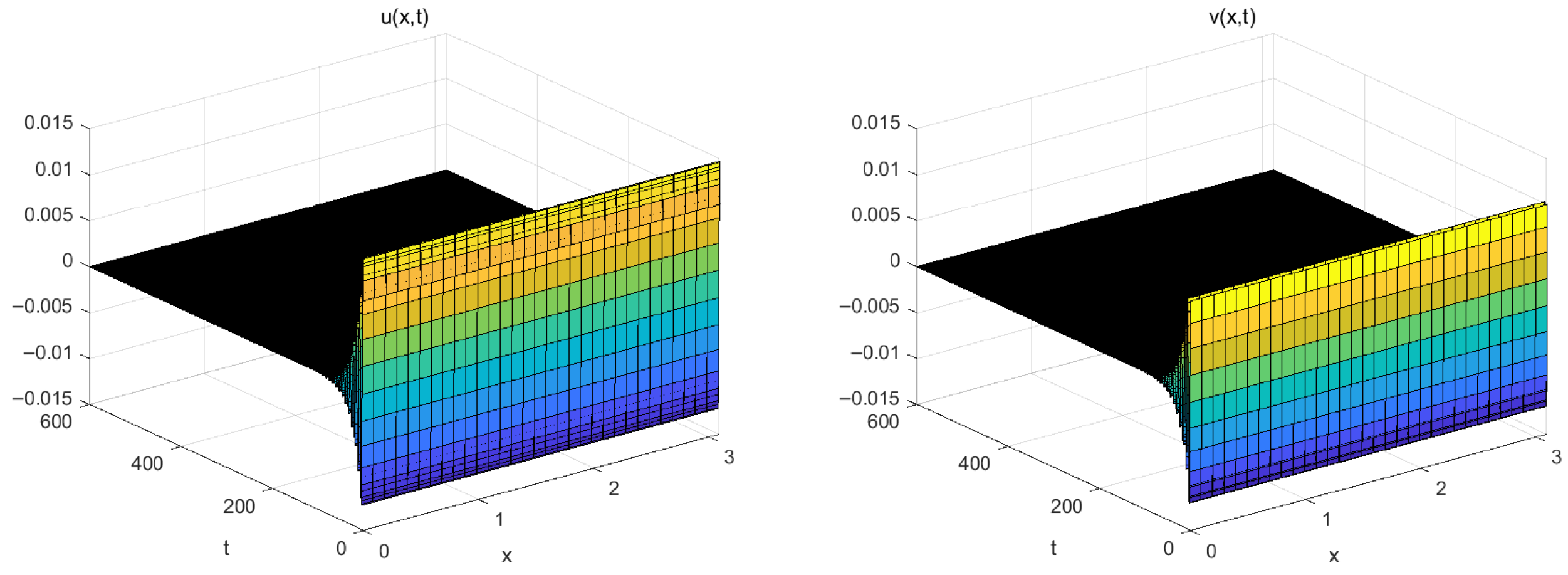
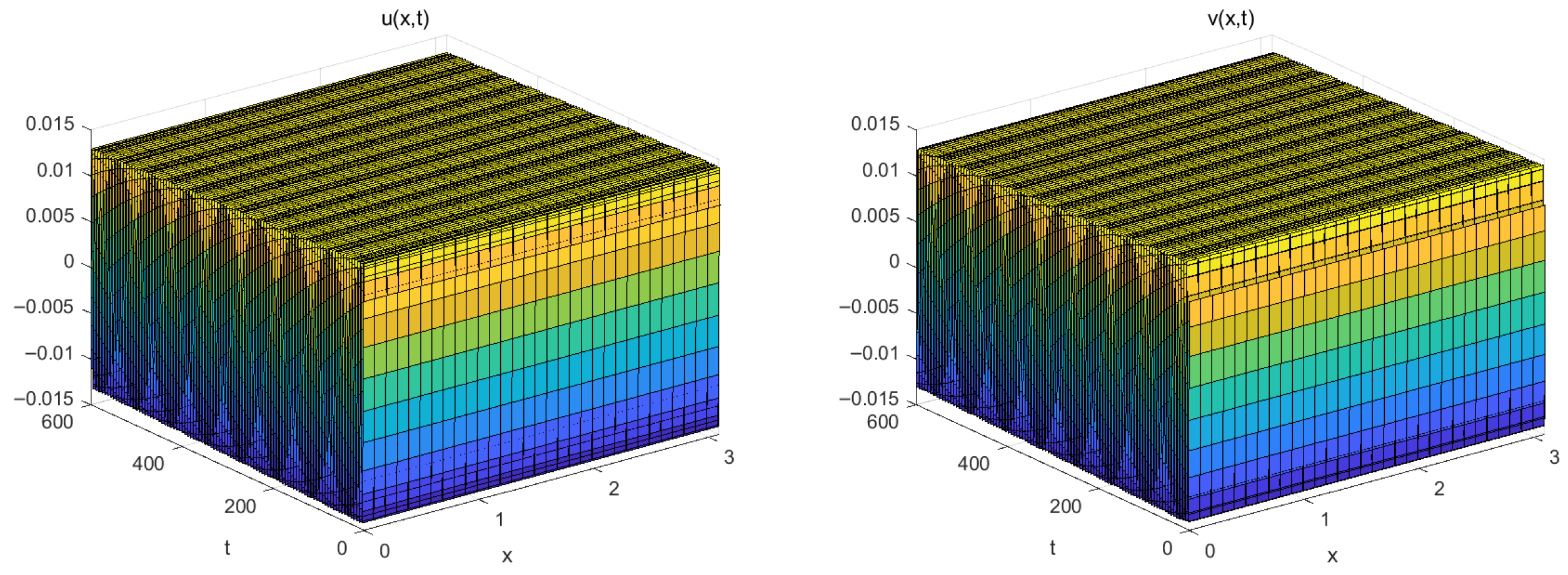
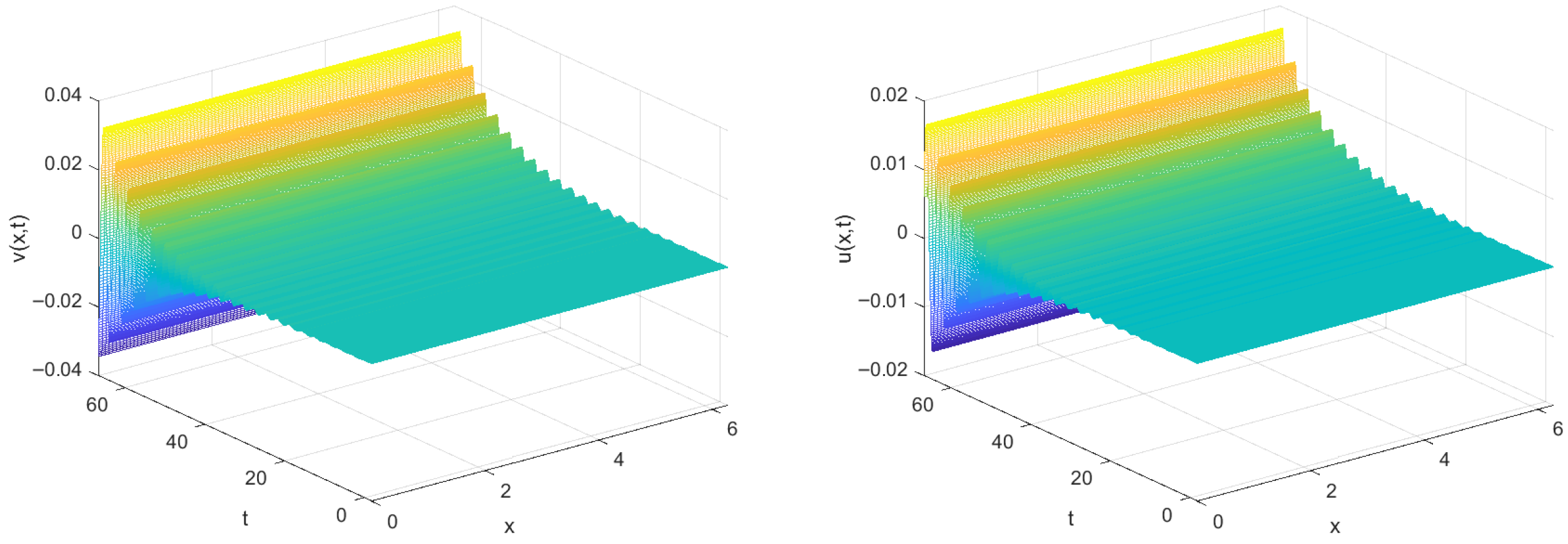
By computing, we obtain $f^{\prime }\left(0\right)=-0.1<0$ and $K_1+K_2=-0.8<0$. According to Theorem 2, system (5) is locally asymptotically stable at $P_0=\left(u_0,v_0\right)=(0,0)$, as shown in Figure 1.

Figure 1. The initial value is $(0.015,0.01)$; $P_0=(0,0)$ is locally asymptotically stable.

Case 2. We take the parameter values as

$$d_1=0.3,d_2=0.5,K_1=-1.2,K_2=0.4,h_1=0.5,h_2=0.1,h_3=-0.1.$$

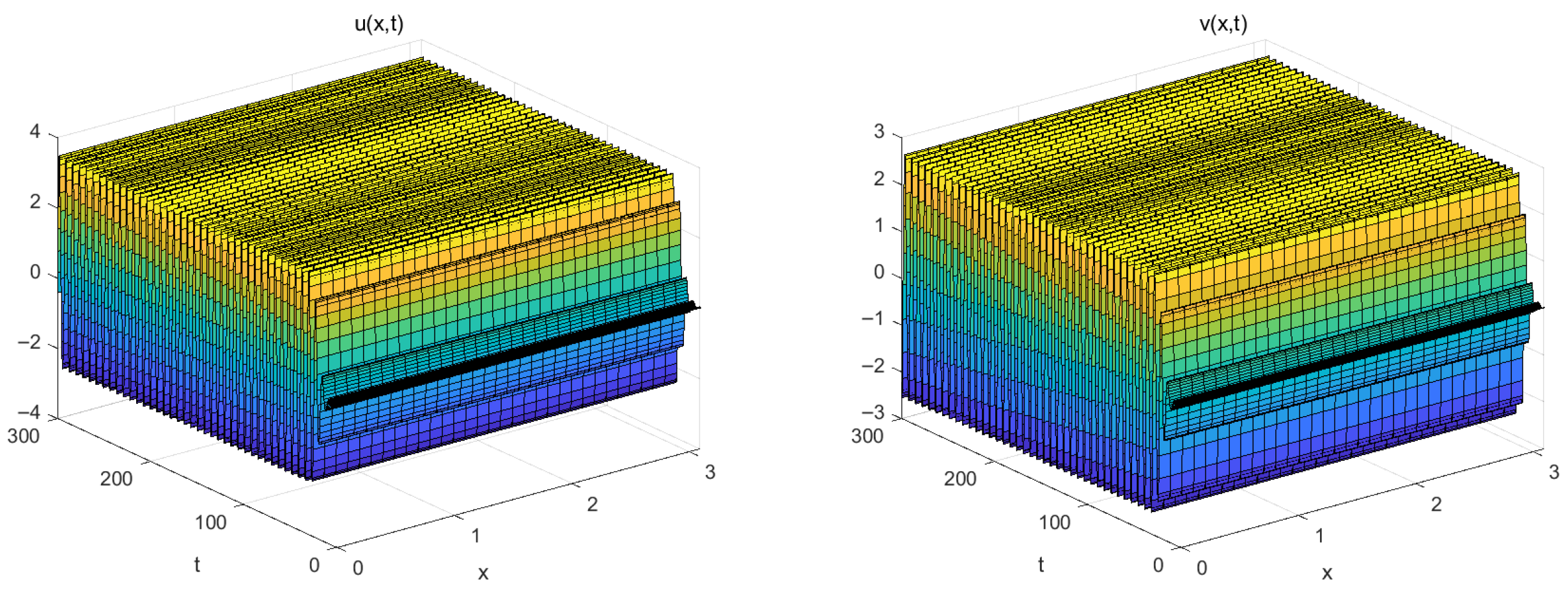
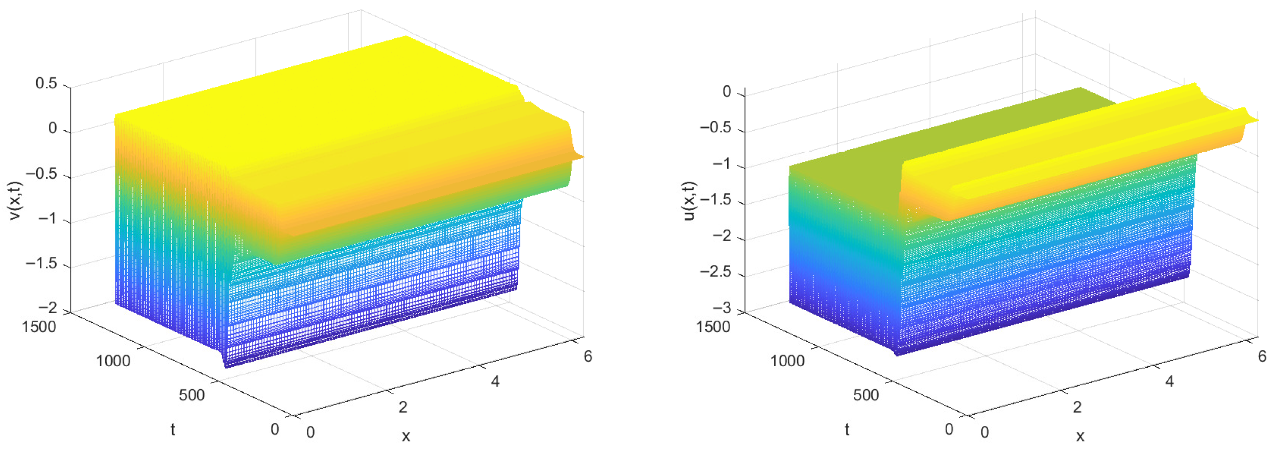
By computing, we obtain $f^{\prime }\left(0\right)=0.5>0$. According to Theorem 2, system (5) is unstable at $P_0=\left(u_0,v_0\right)=(0,0)$, as shown in Figure 2.

Figure 2. $d_1=0.3,d_2=0.5$, and the initial value is $(0.015,0.01)$; the system produces periodic solutions.

Case 3. We take the parameter values as

$$d_1=1,d_2=0.5,K_1=0.1,K_2=0.4,h_1=-0.1,h_2=0.1,h_3=0.1.$$

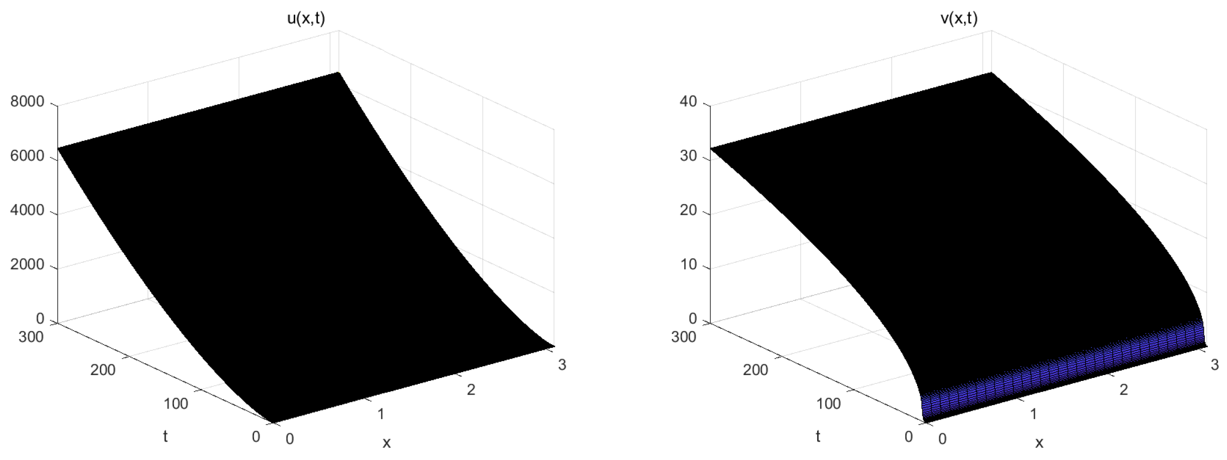
By computing, we have $K_1+K_2=0.5>0$. According to Theorem 2, system (5) is unstable at $P_0=\left(u_0,v_0\right)=(0,0)$, as shown in Figure 3.

Figure 3. $K_1+K_2=0.5>0$, and the system is unstable at $P_0=(0,0)$.

E.g., 5.2. In system (5), we select $f\left(v(x,t)\right)=\gamma \left(e^{av(x,t)}-1\right)-cv(x,t),\tau =0$; then it becomes the most widely used exponential model with Stribeck velocity in engineering. The numerical simulations of a semilinear parabolic Stribeck friction system are performed in the following three cases.

Case 1. Select the parameters as

$$d_1=1,d_2=0.5,K_1=-1.625,K_2=0.625,\gamma =-0.045,a=10,c=0.05.$$

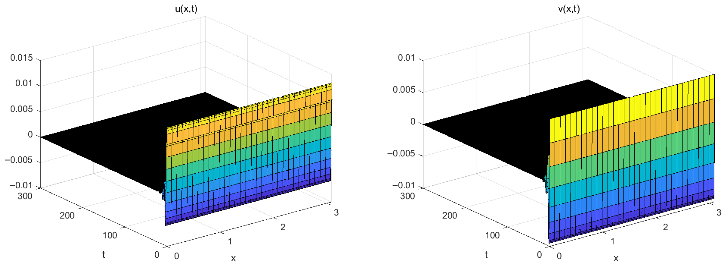
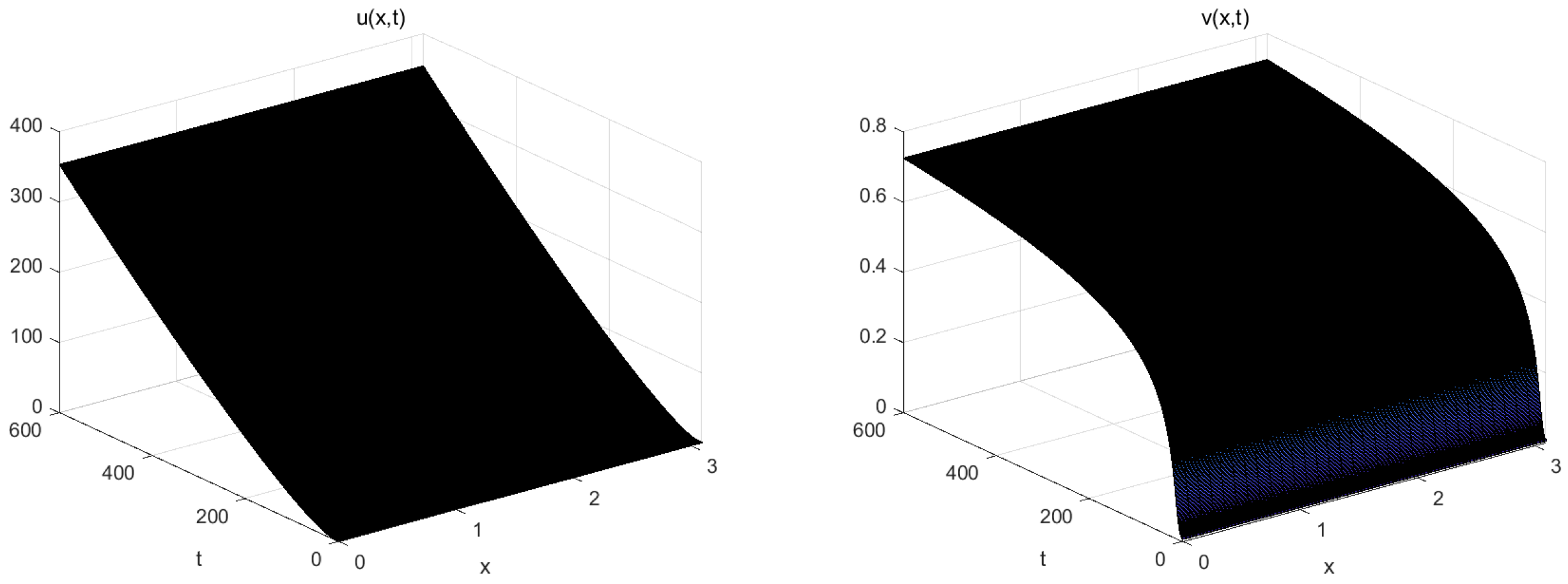
By computing, we obtain $f^{\prime }\left(0\right)=\gamma a-c=-0.5<0$ and $K_1+K_2=-1<0$. According to Theorem 2, system (5) is locally asymptotically stable at $P_0=\left(u_0,v_0\right)=(0,0)$, as shown in Figure 4.

Figure 4. $d_1=1,d_2=0.5$, and the initial value is $(0.015,0.01)$; $P_0=(0,0)$ is locally asymptotically stable.

Case 2. Select the parameters as

$$d_1=0.25,d_2=0.5,K_1=-1.625,K_2=0.625,\gamma =-0.01,a=10,c=-0.101.$$

By computing, we obtain $f^{\prime }\left(0\right)=\gamma a-c=0.001>0$. According to Theorem 2, system (5) is unstable at $P_0=\left(u_0,v_0\right)=(0,0)$, and the stable periodic solutions bifurcate from the equilibrium, as shown in Figure 5.

Figure 5. $d_1=0.23,d_2=0.5$, and the initial value is $(0.015,0.01)$; the system produces periodic solutions.

Case 3. Select the parameters as

$$d_1=1,d_2=0.5,K_1=1,K_2=1,\gamma =-0.5,a=10,c=1.$$

By computing, we obtain $K_1+K_2=2>0$. According to Theorem 2, system (5) is unstable at $P_0=\left(u_0,v_0\right)=(0,0)$, as shown in Figure 6.

Figure 6. $K_1+K_2=0.5>0$ and the initial value is $(0.015,0.01)$; the system is unstable at $P_0=(0,0)$.

2. Stability switch induced by time delay

E.g., 5.3. In system (5), we let $f\left(v(x,t)\right)=h_{1}v(x,t)+h_2{v}^2(x,t)+h_3{v}^3(x,t)$ and select the following parameters:

$$d_1=1,d_2=0.5,K_1=-1.625,K_2=0.625,\gamma =-0.045,a=10,c=0.05.$$

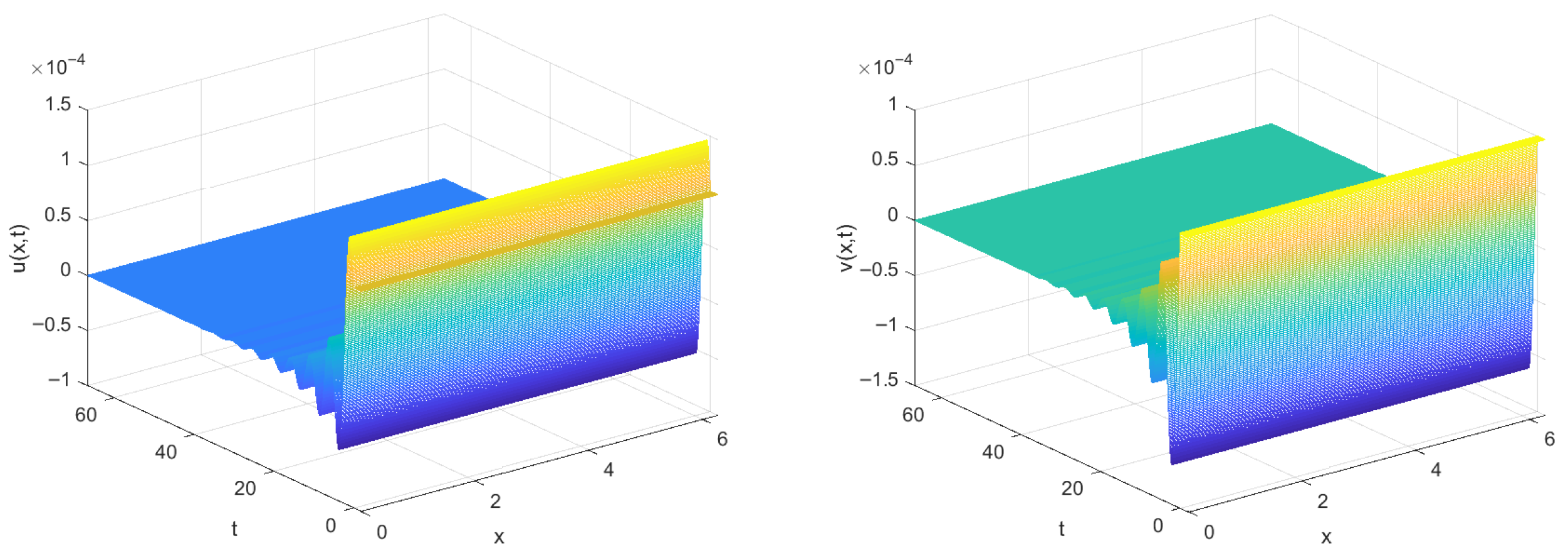
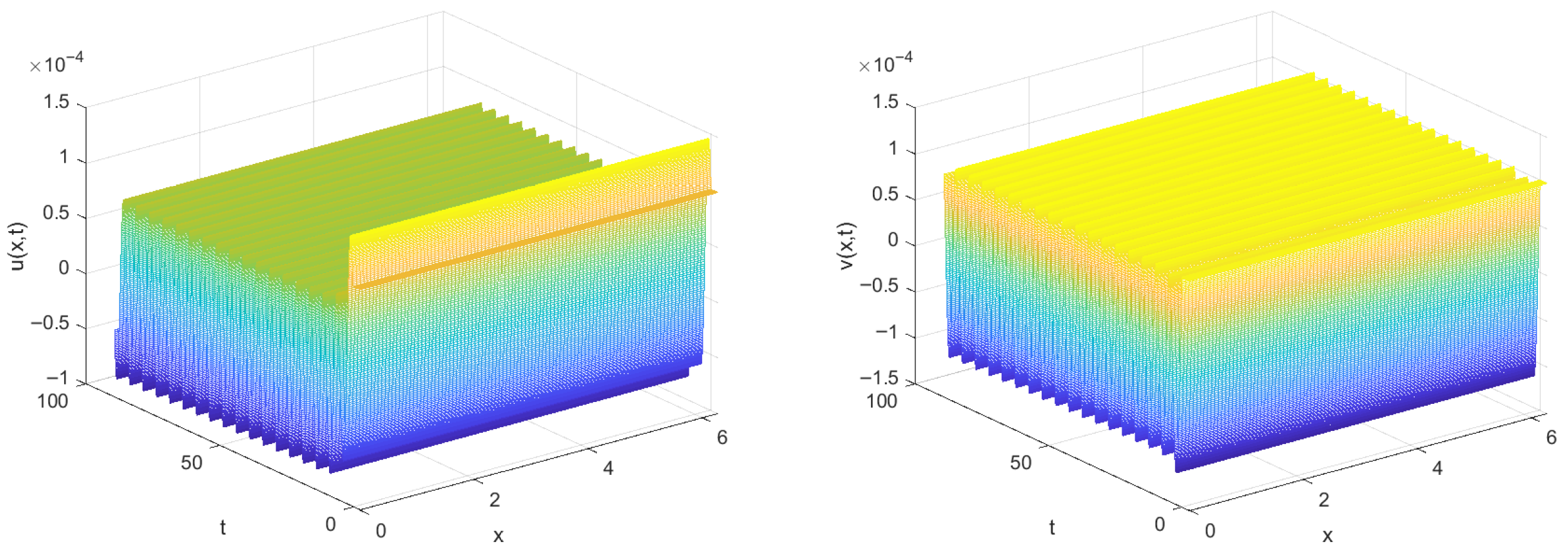
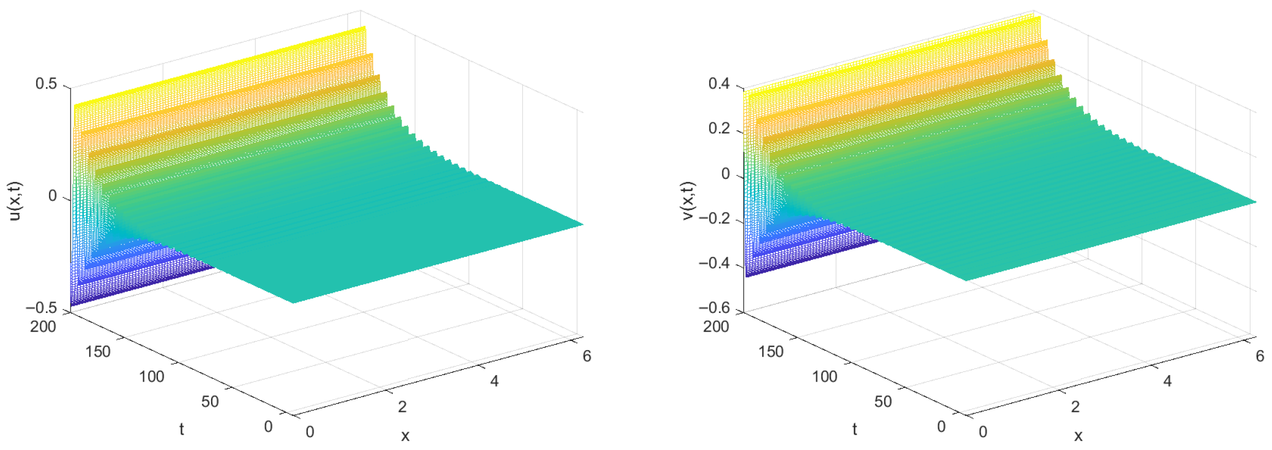
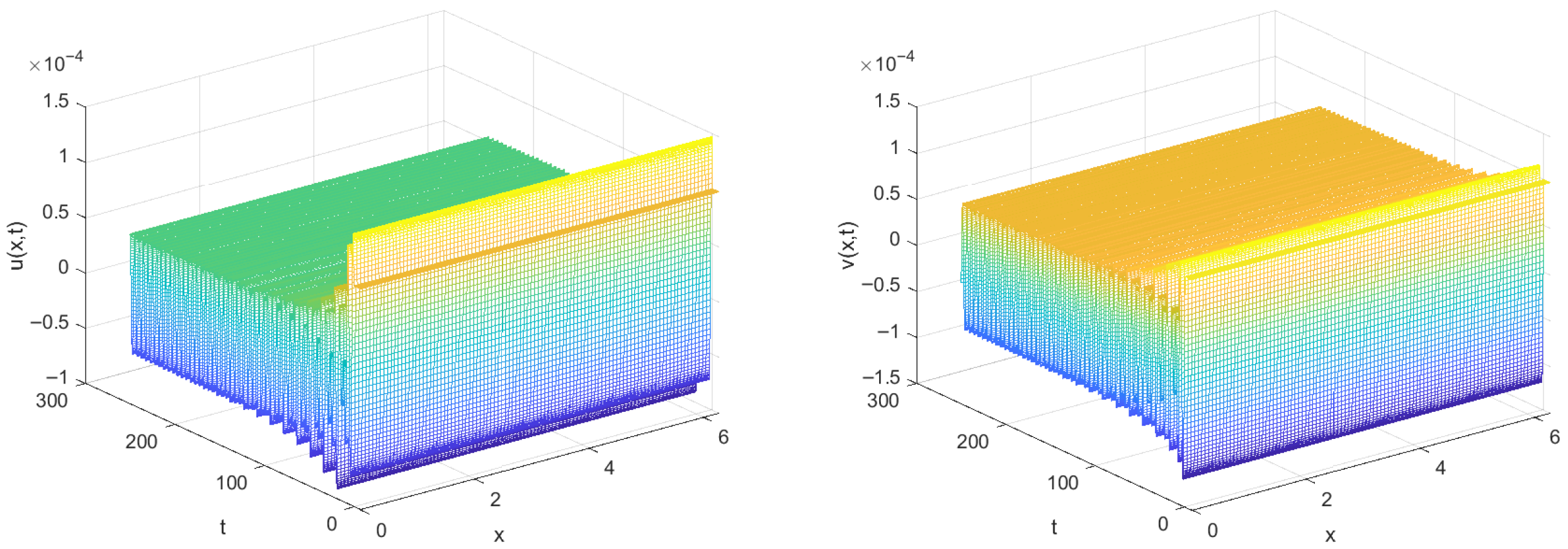
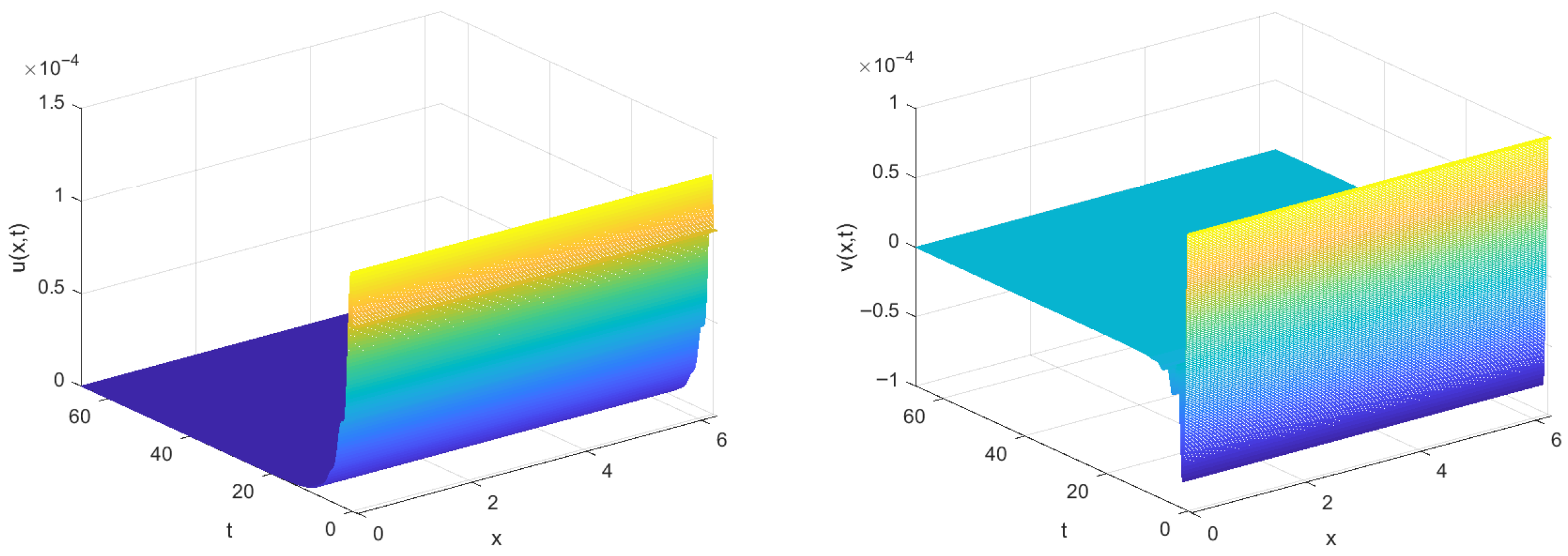
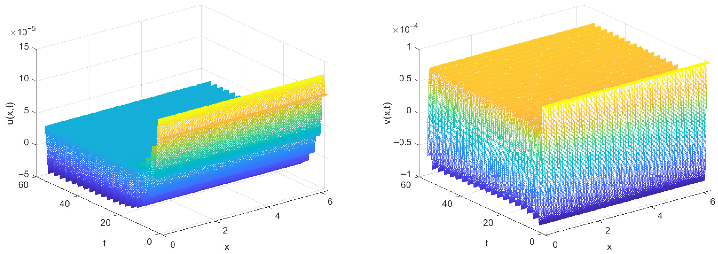
Let $\mathsf{\Omega }=(0,2\pi )$, i.e., $l=2$, By calculation, at the equilibrium $P_0=(0,0)$, ${\tau }_{1,0}^{+}\doteq 2.362<{\tau }_{1,0}^{-}\doteq 2.937<{\tau }_{1,1}^{+}\doteq 7.324$. When ${\tau }_{1,0}^{-}<{\tau }_{1,1}^{+}$, by theorem, $P_0=(0,0)$ is locally asymptotically stable for $\tau \in \left(0,{\tau }_{1,0}^{+}\right)\bigcup \left({\tau }_{1,0}^{-},{\tau }_{1,1}^{+}\right)$ and unstable for $\tau \in \left({\tau }_{1,0}^{+},{\tau }_{1,0}^{-}\right)\bigcup \left({\tau }_{1,1}^{+},+\infty \right)$. When $\tau$ crosses ${\tau }_{1,0}^{\pm }$, the equilibrium $P_0=(0,0)$ loses its stability, and Hopf bifurcation occurs. Additionally, the direction is forward (backward) at $\tau ={\tau }_{1,j}^{+}\left(\tau ={\tau }_{1,j}^{-}\right), j\in {\mathbb{N}}_0$, and the periodic solutions are stable at ${\tau }_{1,0}^{\pm }$. The stability of the equilibrium will change with $\tau$, and there exists “stability switch” in the system, as shown in Figure 7, Figure 8, Figure 9 and Figure 10.

Figure 7. $\tau =2$; $P_0=(0,0)$ is locally asymptotically stable.

Figure 8. $\tau =2.675$; the stable periodic solutions bifurcate from $P_0=(0,0)$.

Figure 9. $\tau =6$; $P_0=(0,0)$ is locally asymptotically stable.

Figure 10. $\tau =7.5$; the stable periodic solutions bifurcate from $P_0=(0,0)$.

E.g., 5.4. In system (5), let $f\left(v(x,t)\right)=\gamma \left(e^{av(x,t)}-1\right)-cv(x,t)$, select the following parameters:

$$d_1=1,d_2=0.5,K_1=-3,K_1=2,{\gamma }_1=-0.045,a=10,c=0.05.$$

Let $l=2$, by calculation, at the equilibrium $P_0=(0,0)$, ${\tau }_{1,0}^{+}\doteq 1.223<{\tau }_{1,0}^{-}\doteq 1.835<{\tau }_{1,1}^{+}\doteq 4.128$. When ${\tau }_{1,0}^{-}<{\tau }_{1,1}^{+}$, by theorem, $P_0=(0,0)$ is locally asymptotically stable for $\tau \in \left(0,{\tau }_{1,0}^{+}\right)\bigcup \left({\tau }_{1,0}^{-},{\tau }_{1,1}^{+}\right)$ and unstable for $\tau \in \left({\tau }_{1,0}^{+},{\tau }_{1,0}^{-}\right)\bigcup \left({\tau }_{1,1}^{+},+\infty \right)$. The stability of the equilibrium will change with $\tau$; there exists “stability switch” in the system, as shown in Figure 11, Figure 12, Figure 13 and Figure 14.

Figure 11. $\tau =1$; $P_0=(0,0)$ is locally asymptotically stable.

Figure 12. $\tau =1.68$; the stable periodic solutions bifurcate from $P_0=(0,0)$.

Figure 13. $\tau =2$; $P_0=(0,0)$ is locally asymptotically stable.

Figure 14. $\tau =4.5$; the stable periodic solutions bifurcate from $P_0=(0,0)$.

6. Conclusions

This paper performs an in-depth dynamic analysis of a semilinear parabolic friction system incorporating the diffusion effect and time-delayed feedback control. Theoretical analysis reveals that stability can switch multiple times as the delay varies. This finding demonstrates that time-delayed friction systems exhibit richer dynamic characteristics compared to systems without time delays. The conclusions of this study have clear significance in engineering applications; the established stability criteria and bifurcation formulae can provide a critical theoretical basis for predicting and suppressing frictional vibration caused by time-delayed feedback in practical mechanical systems. This research not only deepens the understandings of the complex dynamics of friction systems under the coupled time delay and diffusion effects, but also provides a solid theoretical foundation and practical analytical tool for solving vibration control problems in relevant engineering fields.

References

- Canudas, d.W.C.; Olsson, H.; Astrom, K.J. A new model for control of systems with friction. IEEE Trans. Autom. Control 1995, 40, 419–425. [Google Scholar] [CrossRef] [Scilit]
- Dupont, P.; Hayward, V.; Armstrong, B. Single state elastoplastic friction models. IEEE Trans. Autom. Control 2002, 47, 787–792. [Google Scholar] [CrossRef]
- Hinrichs, N.; Oestreich, M.; Popp, K. On the Modeling of Friction Oscillators. J. Sound Vib. 1998, 216, 435–459. [Google Scholar] [CrossRef] [Scilit]
- Lampaert, V.; Swevers, J.; Al-Bender, F. Modification of the Leuven integrated friction model structure. IEEE Trans. Autom. Control 2002, 47, 683–687. [Google Scholar] [CrossRef] [Scilit]
- Lampaert, V.; Al-Bender, F.; Swevers, J. A generalized Maxwell-slip friction model appropriate for control purposes. In Proceedings of the 2003 IEEE International Workshop on Workload Characterization (IEEE Cat. No. 03EX775), St. Petersburg, Russia, 20–22 August 2003; Volume 4, pp. 1170–1177. [Google Scholar]
- Mcmillan, A.J. A Non-Linear Friction Model For Self-Excited Vibrations. J. Sound Vib. 1997, 205, 323–335. [Google Scholar] [CrossRef] [Scilit]
- Panovko, Y.G.; Gubanova, I.I. Stability and Oscillations of Elastic Systems, Paradoxes. In Fallacies and New Concepts; Consultants Bureau: New York, NY, USA, 1965. [Google Scholar]
- Ruina, A. Slip Instability and State Variable Friction Laws. J. Geophys. Res. Atmos. 1983, 881, 10359–10370. [Google Scholar] [CrossRef] [Scilit]
- Swevers, J.; Al-Bender, F. An integrated friction model structure with improved presliding behavior for accurate friction compensation. IEEE Trans. Autom. Control 2000, 45, m675–m686. [Google Scholar] [CrossRef] [Scilit]
- Thomsen, J.J. Using Fast Vibrations to Quench Frictioninduced Oscillations. J. Sound Vib. 1999, 228, 1079–1102. [Google Scholar] [CrossRef] [Scilit]
- Hale, J.K. Theory of Functional Differential Equations; Springer: New York, NY, USA, 1977. [Google Scholar]
- Maccari, A. Vibration control for the primary resonance of a cantilever beam by a time delay state feedback. J. Sound Vib. 2003, 259, 241–251. [Google Scholar] [CrossRef] [Scilit]
- Maccari, A. Vibration control for parametrically excited Linard systems. Int. J. Non-Linear Mech. 2006, 41, 146–155. [Google Scholar] [CrossRef] [Scilit]
- Li, X.; Ji, J.C.; Hansen, C.H. The response of a Duffing-van der Pol oscillator under delayed feedback control. J. Sound Vib. 2006, 291, 644–655. [Google Scholar] [CrossRef] [Scilit]
- Yi, F.; Wei, J.; Shi, J. Bifurcation and spatiotemporal patterns in a homogeneous diffusive predator-prey system. J. Differ. Equ. 2009, 246, 1944–1977. [Google Scholar] [CrossRef] [Scilit]
- Pyragas, K. Control of Chaos by Self-Controlling Feedback. Phys. Lett. A 1992, 170, 421–428. [Google Scholar] [CrossRef] [Scilit]
- Song, Y.; Wei, J. Bifurcation analysis for Chen’s system with delayed feedback and its application to control of chaos. Chaos Solitons Fractals 2004, 22, 75–91. [Google Scholar] [CrossRef] [Scilit]
- Wang, H.; Liu, J. Stability and bifurcation analysis in a magnetic bearing system with time delays. Chaos Solitons Fractals 2005, 26, 813–825. [Google Scholar] [CrossRef] [Scilit]
- Wei, J.; Jiang, W. Stability and bifurcation analysis in Van der Pol’s oscillator with delayed feedback. J. Sound Vib. 2005, 283, 801–819. [Google Scholar] [CrossRef] [Scilit]
- Faria, T. Stability and Bifurcation for a Delayed Predator-Prey Model and the Effect of Diffusion. J. Math. Anal. Appl. 2001, 254, 433–463. [Google Scholar] [CrossRef] [Scilit]
- Li, W.T.; Yan, X.P.; Zhang, C.H. Stability and Hopf bifurcation for a delayed cooperation diffusion system with Dirichlet boundary conditions. Chaos Solitons Fractals 2008, 38, 227–237. [Google Scholar] [CrossRef] [Scilit]
- Yan, P.; Li, W.T. Bifurcation and global periodic solutions in a delayed facultative mutualism system. Phys. D Nonlinear Phenom. 2007, 227, 51–69. [Google Scholar] [CrossRef] [Scilit]
- Saha, A.; Bhattacharya, B.; Wahi, P. A comparative study on the control of friction-driven oscillations by time-delayed feedback. Nonlinear Dyn. 2010, 60, 15–37. [Google Scholar] [CrossRef] [Scilit]
- Hassard, B.D.; Kazarino, N.D.; Wan, Y.H. Theory and Applications of Hopf Bifurcation; Cambridge University: Cambridge, UK, 1981. [Google Scholar]
- Wu, J. Theory and Applications of Partial Functional Differential Equations; Springer: New York, NY, USA, 1996. [Google Scholar]
- Faria, T. Normal Forms and Hopf Bifurcation for Partial Differential Equations with Delays. Trans. Am. Math. Soc. 2000, 352, 2217–2238. [Google Scholar] [CrossRef] [Scilit]
Disclaimer/Publisher’s Note: The statements, opinions and data contained in all publications are solely those of the individual author(s) and contributor(s) and not of MDPI and/or the editor(s). MDPI and/or the editor(s) disclaim responsibility for any injury to people or property resulting from any ideas, methods, instructions or products referred to in the content. |
© 2025 by the authors. Licensee MDPI, Basel, Switzerland. This article is an open access article distributed under the terms and conditions of the Creative Commons Attribution (CC BY) license.