


Abstract
Mineralogical data acquired from drillcores provide important constraints for resource estimation, geometallurgical modelling, mineral exploration, and geological interpretation. While hyperspectral imaging is rapidly gaining traction for these applications, it lacks the ability to accurately quantify mineral abundances without extensive calibration data. Here, we build on previous work to demonstrate and benchmark workflows that combine scanning electron microscope (SEM) mineral maps with large-extent multimodal hyperspectral imaging data. The goal is to relate hyperspectral features and mineral abundances using supervised machine learning models, and then apply these models to infer mineralogy across entire drillcores. We adapt the learning process to the non-uniform (unbalanced) composition of most rocks, and achieve reasonable accuracy for most rock-forming minerals. However, we also find that prediction accuracy depends strongly on the representativity of training data—so models often fail to produce accurate maps of rare and accessory minerals. Robust, adaptive and ideally semi-automated sampling approaches might address this shortcoming by identifying locations which ensure optimal coverage of hyperspectral variance. We also emphasise that upscaling from SEM to drillcore scale inevitably involves extrapolation, meaning predictions should always be validated. However, once validated, upscaled mineralogy predictions could provide crucial quantitative data that bridge the scale gap between petrographic observations, metallurgical tests, and geometallurgical models.
1. Introduction
Hyperspectral drillcore imaging data is becoming widely used in the resource sector, with diverse applications across mineral exploration [1,2,3,4], geometallurgy [5,6,7], mine-face mapping [1,6,8,9], and sensor-based sorting for primary [10,11] and secondary [12] resource streams. These applications take advantage of hyperspectral imaging sensors’ ability to rapidly acquire continuous data at high spatial resolution (mm–cm) over large areas (tens to hundreds of kilometers of drillcore). The resulting ‘big data’ contains many hundreds of highly correlated spectral bands, capturing absorption or emission features characteristic of a wide range of materials, including minerals (see [13] for a detailed review).
However, hyperspectral data are often ambiguous because identical spectra can result from multiple minerals, and spectral response depends additionally on texture and surface properties (grain size, roughness, etc. [14,15]). This ambiguity makes the link between mineralogy and hyperspectral data non-unique in two directions: a single composition can have many spectral responses, and an observed spectrum can result from many mineral mixtures.
For example, many carbonate minerals can be characterised using the C-O absorption between ~2300–2350 nm (calcite and dolomite end-members, although Fe-, Mn-, and Mg- can also shift this feature [13]). Clay minerals often also show an absorption in this range, complicating the interpretation of mixtures. Further challenges arise as the depth and shape of carbonate (and clay) absorptions also change as texture, grain size and surface properties vary [14,16,17].
Expert-based approaches can be applied to map specific spectral features and interpret useful qualitative information on mineralogy [18,19,20,21,22,23,24,25] or characterise overall variability [26,27]. These simpler methods have the advantage that training information is not strictly needed, but require careful interpretation to resolve ambiguities. Established feature-mapping or unmixing methods can also be challenging to apply across broad spectral ranges, due to inherently different information provided by, e.g., the shortwave vs. longwave infrared [25].
While these challenges can be overcome in simple systems, quantification of complex mineralogy requires a supervised-learning approach. Several studies have demonstrated this potential, using coregistered hyperspectral and mineralogical information to derive locally accurate mineralogy predictions [11,28,29]. However, the application of supervised learning techniques to large drillhole databases requires methods that can handle (1) the large amounts of data involved, and (2) extended range spectra needed to reduce non-uniqueness and facilitate extrapolation and upscaling. Differences between training samples and drillcore scans (in, e.g., illumination, topography or surface roughness) can also present challenges, especially if the scanned drillcores are uncut.
In this contribution, we present a diverse and extended-spectral range benchmark dataset for testing emerging machine learning approaches. The dataset contains SEM-mineralogy and coregistered visible-near (VNIR; 350–900 nm), short-wave (SWIR; 900–2500 nm), mid-wave (MWIR; 3000–5200 nm) and long-wave (LWIR; 7000–12,000 nm) infrared spectra for 206 thick-section billets sampled across hyperspectrally scanned drillcores from diverse locations and geological settings. We also complement these data with an open-source Python (v3.8.13) package (hklearn; http://github.com/hifexplo/hklearn, accessed on 10 June 2026) that aims to facilitate usage and help further the development of robust machine learning-based upscaling methods.
1.1. Pixel-Scale Predictions
Hyperspectral upscaling (Figure 1) is a technique by which localised high-spatial resolution measurements are used to train regression or classification models that predict across much larger areas covered by hyperspectral data [3,29,30]. In the context of this paper, the target variable is mineralogy, although promising attempts have recently been made to predict other physical, chemical, and mechanical rock properties [5,15,31,32,33,34]. Supervised hyperspectral regression or classification tasks have also been applied in a similar way to upscale local information in ecology [35,36,37], soil science [38,39,40] and agriculture [41,42].
Figure 1.
Schematic outline of the hyperspectral upscaling workflow, in which detailed SEM mineralogy data are used to make predictions across a large database of hyperspectrally scanned drillcores. Values of n show the approximate number of data involved in each step, emphasising the significant change in spatial extent when upscaling localised mineralogy information across large drillcore datasets.
Various machine learning approaches have been deployed to predict mineralogy from hyperspectral data. These can be grouped into three broad categories: pixel classification, spectral unmixing, and regression of mineral composition. Classification approaches assign each hyperspectral measurement (pixel) to a specific class, typically the most abundant mineral phase [18,19,29,43,44,45,46]. While the low dimensionality of the prediction (class ID) is easier to visualise and makes the learning task simpler, accessory phases that are rarely (or never) the most abundant phase can be systematically underestimated.
Spectral unmixing approaches decompose pixel spectra into a weighted sum of endmembers, each representing a pure mineral. When training data are available, a least-squares estimation of the pure endmember spectra can be made [3,47] and then applied to unknown data to predict mineralogy. While the simplicity and interpretability of this approach are attractive, nonlinear spectral mixing effects and varying response across extended spectral ranges pose significant challenges. For example, minerals that dominate spectral response in the SWIR range often differ from those that determine LWIR signal [25,48]. Unmixing is also often posed as the least-squares minimisation of residuals across many hyperspectral bands, giving results that are more influenced by broad spectral features than the narrow absorptions characteristic of specific mineral groups.
Finally, multivariate regression approaches model the relationship between spectral data and mineral abundance [11,28]. Although theoretically robust, regression methods also face several challenges. Firstly, mineral abundance data are compositional, meaning model predictions should sum to one, introducing a closure problem that requires all minerals to be predicted simultaneously. Secondly, minerals often occur in associations, making it impossible for algorithms to accurately learn individual minerals’ spectral features unless pure pixels are present in the training set, or data from diverse settings are included (to break these associations). Finally, mineral abundances often exhibit extremely skewed distributions, including many true zeroes, making it difficult to apply established compositional data approaches and to derive loss functions that are not strongly biased towards more abundant phases.
1.2. Aggregate Predictions
It is important to note at this point that most applications of hyperspectral (drillcore) mineralogy involve an aggregation or averaging of predicted compositions into larger (e.g., 1 m) intervals or geometallurgical domains. This averaging can reduce some of the errors that occur in individual pixel predictions, though systematic biases (e.g., under-prediction of low-abundance phases) can also remain. Regardless of the approach applied, the distinction between pixel-scale and interval- or domain-scale predictions should be considered when evaluating accuracy and validating results.
In this study (and benchmark), we compare modal mineralogy at both pixel and aggregated thick-section billet scale. Real applications would ideally also include further validation derived from bulk mineralogy measurements (e.g., X-ray diffraction (XRD)) of larger (multi-meter) drillcore intervals. Comparison against bulk measurements can also identify potential biases between surface-area and volume-based composition estimates.
2. Methods
2.1. Sample Set and Geological Context
Samples from drillholes intersecting a diverse range of geological settings were compiled for use in this study (Table 1), to create a dataset capturing the hyperspectral characteristics of minerals in many different mixtures and rock types. These sites include Variscan crystalline basement (three regions from Saxony, Germany, and one from the Massif Central, France) and Paleozoic sedimentary cover from Spremberg (Permian Basin, Germany) and the Irish Midlands (Stonepark and Collinstown, Ireland).
Table 1.
Summary of the amount of drillcore scanned and number of sampled thick-section billets at each study site. The resulting breadth of covered lithology is also described.
Each sample was cut into a 25 mm × 40 mm thick-section billet and lapped to a 3 mm thickness. This relatively thick sample dimension was necessary to limit section transparency, a common problem when conducting hyperspectral scans of conventional thin sections. Superglue was used for adhesion instead of epoxy resin to reduce spectral interference and minimise infiltration into pore spaces.
Hyperspectral data were collected across the unpolished thick-section billets using a SiSuROCK drillcore scanner (Specim; Oulu, Finland), following the workflow described by [49]. Most samples appeared completely opaque during scanning, with the exception of some quartz-rich lithologies. These thick-section billets were placed on a Spectralon white panel prior to scanning to limit spectral interference from underlying material.
2.1.1. Spremberg (Germany)
A total of 25 thick-section billets were prepared for Mineral Liberation Analysis (MLA) from three mineralised drillcores extracted from the Spremberg–Graustein Kupferschiefer exploration zone (Lusatia, Germany) by Kupferschiefer Lausitz (KSL) between 2009 and 2010. These samples comprise Weissliegend and Rotliegend sandstones, Zechstein Kupferschiefer mudstone, and overlying Zechstein limestone/dolostone. The suite thus captures the mineralised Kupferschiefer horizon and its immediate footwall red-bed sandstones and hanging-wall carbonates, representative of the stratabound Cu–Ag system of the Central European Kupferschiefer basin [4,50,51].
2.1.2. Collinstown (Ireland)
Cores from five holes drilled by Teck Ireland in the Collinstown Zn–Pb prospect (Lower Carboniferous Irish Midlands Basin, County Westmeath, Ireland) were sampled to prepare a total of 30 thick-section billets. The sampled stratigraphy includes Upper Dark Limestones of the Lucan Formation, the Feltrim Formation (Boulder Conglomerate), argillaceous bioclastic limestones of the Slane Castle Formation, shaley pale limestones of the Meath Formation, mixed beds of the Liscarton Formation, and underlying Lower Palaeozoic basement rocks. The suite captures variable sedimentary facies, dolomitisation, structurally controlled hydrothermal alteration and mineralisation, typical of epigenetic Irish-type Zn–Pb systems emplaced during burial diagenesis in carbonate platforms [52,53].
2.1.3. Stonepark (Ireland)
A total of 44 thick-section billets were prepared from four drillholes at the Stonepark prospect, County Limerick, Ireland, drilled by Group Eleven Resources. The sampled lithologies comprise Waulsortian Limestone (mudbank facies), argillaceous bioclastic limestones of the Ballysteen Formation, cherty mudstones of the Lough Gur Formation, and volcanic rocks of the Knockroe and Knockseefin formations (basalts, tuffs and intrusive dykes). Mineralisation is hosted within hydrothermal dissolution breccias developed in the lower Waulsortian Limestone and consists of pyrite–marcasite, sphalerite, and galena with Fe-dolomite and calcite gangue, representing an epigenetic Irish-type Zn–Pb system spatially associated with intrusive rocks [54].
2.1.4. Massif Central (France)
Cores extracted by Imerys Beauvoir from the Li-Sn-W-rich Beauvoir granite were sampled to prepare 47 thick-section billets. All samples are thus granitic, though they present variation in lithium mica (lepidolite) content and alteration style and intensity. Early stages of greisenisation at Beauvoir consist of albitisation followed by the partial or complete breakdown of the feldspars and their replacement by quartz and muscovite. Phosphorus is brought into the system during this alteration, and lepidolite appears to be replaced by muscovite and secondary lithium minerals like montebrasite. Late low-temperature kaolinitisation and hematitisation are present in confined, often previously greisenised, zones [55].
2.1.5. Freiberg District (Germany)
A total of 20 thick-section billets were prepared from gneiss, meta-sedimentary and meta-igneous rocks intersected by four exploration drillholes in the northern Freiberg district, drilled by Excellon Resources in 2020. The meta-igneous rocks include silicified mafic to ultra-mafic (meta-gabbro, serpentinite) and volcanic (basalts and volcano-sedimentary) lithologies. Several of the gneisses are also altered, likely by high-temperature fluids associated with latest-Carboniferous to early-Permian epithermal Ag-Pb-Zn veins [56,57,58].
2.1.6. Schönbrunn/Bösenbrunn (Germany)
Twenty samples were selected from two exploration holes (SbrOV 7/73 and Bou 21/77) drilled in the 1970s by VEB Geologische Erkundung und Forschung through the Schönbrunn/Bösenbrunn fluorite deposits, southwestern Vogtland (hereafter referred to as Bösenbrunn for clarity). The samples are composed of lapilli- and ash-tuffs, basalt flows, and clastic sedimentary rocks that locally underwent low-grade metamorphism [59]. The sequence is spatially associated with concealed granitic intrusions and cut by structurally controlled fluorite-bearing veins [59]. The Eichigt–Schönbrunn apical granite shows pervasive hydrothermal alteration, interpreted to be genetically linked to the fluorite mineralisation [60].
2.1.7. Geyer (Germany)
Finally, 20 thick-section billets were prepared from drillhole Z606A1/2011 at the Geyer SW skarn deposit (Erzgebirge, Germany), drilled by Deutsche Rohstoff AG in 2011. Sampled lithologies comprise muscovite and muscovite–biotite schists (locally garnet-bearing) and muscovite gneiss, together with a range of skarn assemblages including pyroxene-, pyroxene–garnet, pyroxene–magnetite, pyroxene–feldspar, and (retrograde) amphibole–chlorite skarn. This paragenetic spectrum reflects a prograde clinopyroxene–garnet skarn stage followed by hydrothermal tin mineralisation and a later retrograde overprint, consistent with recent studies of the Geyer SW deposit [61,62].
2.2. Hyperspectral Data Acquisition and Processing
A SiSuROCK hyperspectral drillcore scanner fitted with cameras covering the visible (RGB-Jai), VNIR-SWIR (AisaFENIX), MWIR (FX50) and LWIR (AisaOWL) spectral ranges was used to acquire 1 mm (FX50) to 1.5 mm (AisaFENIX) spatial resolution hyperspectral data covering drillcores from each of the study areas. Most of these cores were cut and cleaned prior to scanning, and approximately levelled to present a horizontal surface to the scanner. The same instrument (and settings) was used to acquire matching hyperspectral data over the thick-section billets to derive training and testing data. Instrument setup, drillcore data, data collection and preprocessing processes are described in detail in [49].
The real-time processing workflow described by [49] was used to remove lens distortions, dead and blinking pixels, convert to reflectance (relative to a white-reference mounted next to each scanned core box) and coregister data from each sensor to the FX50 image using an affine transform. Background pixels (e.g., core-boxes) were masked using a semi-automatic workflow based on the Segment Anything Model [63,64], followed by manual QAQC and adjustment using a plugin (napari-hippo; [49]) for napari [65].
2.3. Sample Selection
The selection of adequate test and training samples is crucial to successful upscaling and meaningful assessment of prediction accuracy. This can be a significant challenge when working with large numbers of lithologically and/or mineralogically diverse drillcores, as each target mineral needs to be present (in different mixtures) in both the testing and training datasets.
To help mitigate some of these challenges, we developed a novel workflow that uses the hyperspectral data output from the real-time processing workflow [49] to suggest optimal sample locations that (1) cover the spectral diversity observed in one or more scanned drill holes, (2) contain infill samples of intermediate composition that help constrain nonlinear mixing effects, and (3) maximise the spectral diversity (and hence information) within each sample.
Our approach (Figure 2) builds on the method described by [17]. Data for each drillcore box and hyperspectral sensor was passed through a MNF [26] to reduce noise and dimensionality (to 15 components), and a principal component analysis (PCA) applied to the concatenated MNF results to remove intra-sensor correlation and further reduce dimensionality (Figure 2a–c). Superpixels were then defined in this low-dimensional latent space by grouping spatially and spectrally clustered pixels (Figure 2d) using SLIC (Simple Linear Iterative Clustering, a spatially aware k-means classification; [66]).
Figure 2.
Overview of the data-driven sampling workflow. Hyperspectral reflectance images were acquired and processed in real-time (a), then reduced in dimensionality (b,c) to define superpixels (d) and create a drillcore-scale spectral library. A small set of target spectra was then selected from this library by finding extrema (e) and infill points (f) that optimally cover the spectral variance. Finally, a sliding window (g) with dimensions similar to the thick-section billets was used to identify a minimum set of blocks (h) that includes each target spectrum (within a threshold distance) and maximises the sampled spectral diversity (number of superpixels in each block).
Full spectra (concatenated VNIR-SWIR-MWIR-LWIR) were then averaged for each superpixel and added to a library covering the entire drillhole. Target superpixels were then selected from this library using N-FINDR (n-endmembers = samples/2; Figure 2e) and k-means (n-classes = samples/2; Figure 2f). N-FINDR selects superpixels with extreme spectra, while k-means was used in a PCA-reduced component space to identify superpixels closest to the centroid of classes distributed approximately equally through the range of spectral variability. The combination of N-FINDR and k-means selected superpixels provides a small set of target spectra that systematically covers the spread of spectral diversity with a limited number of samples.
Optimally located sample blocks were then found (Figure 2g) using a sliding window (approximately the same size as a thick-section billet) to identify locations that (1) include many superpixels (indicating local spectral diversity/high information content), and (2) contain spectra matching (based on the spectral angle) the target superpixels. This approach fits as much information as possible into each sample while ensuring coverage of the overall spectral diversity.
Finally, hand-sample sized pieces of core were extracted from the suggested locations. To ensure some overlap in the resulting dataset (for subsequent splitting into testing and training subsets), suggestions were generated independently for each sampled drillhole from Spremberg, Stonepark, and Collinstown. Conventional (geologist-based) sampling was applied at the remaining sites because the rapid hyperspectral processing [49] needed to apply the above algorithm was not available during these data acquisition campaigns.
2.4. Sample Preparation and Automated Mineralogy
After hyperspectral scanning, the samples were lightly polished to achieve a smooth surface (while removing as little material as possible), carbon-coated, and analysed using SEM-based MLA. Polishing was conducted after hyperspectral scanning as specular reflections from polished surfaces cause misleading hyperspectral artefacts.
An FEI (Hillsboro, OR, USA) Quanta 650 F field emission SEM equipped with Bruker (Billerica, MA, USA) Quantax X-Flash 5030 energy dispersive X-ray detectors was used to acquire back-scatter electron (BSE) images and energy-dispersive X-ray spectra (EDS) for automated mineral mapping using the MLA software (version 3.1.5). This approach leverages the compositional information in the EDS spectra and density information in the BSE images to predict mineralogy with considerable accuracy.
Two measurement modes were used: Grain-based X-ray mapping (GXMAP) for detailed mineralogical analysis in fine-grained or texturally complex areas, and X-ray modal analysis (XMOD) for determining mineral proportions more rapidly over large areas. The combined EDS and BSE data were then classified using a mineralogical reference list generated separately for each site, and iteratively cross-checked against whole-rock X-ray diffraction (XRD) and X-ray fluorescence data to address uncertainties (e.g., distinguishing illite and muscovite) inherent to the MLA method (cf. Section 4.1, [51]). Lookup tables describing the classes (columns) and corresponding mineral abundances (rows) used for MLA mineral classification at each site are included in the Supplementary Sheets. Finally, the resulting 3 µm resolution mineral classification map was exported to an indexed bitmap format for subsequent processing, including conversion from per-pixel class to per-pixel abundance (cf. Section 2.5).
2.5. MLA Coregistration and Spectral Preprocessing
Classification maps were imported into napari-hippo [49] to coregister them with the RGB drillcore scanner images. The RGB image was used because of its 6 times higher (160 µm) spatial resolution, making keypoint matching easier compared to the ~1 mm resolution hyperspectral data. The matched keypoints were used to find an affine transform aligning data for each thick-section, generally resulting in alignment to within ~3 RGB pixels (0.5 hyperspectral pixels after downsampling). We note that the incomparability between MLA classifications and optical images prevented automated keypoint matching and alignment, and makes it challenging to perform quantitative assessments of coregistration error.
The lookup table describing modal mineralogy for each MLA class (cf. Supplementary Sheets) was then applied to derive mineral abundance images, in which each band represents the modal abundance of one mineral. This was necessary because many fine-grained samples required mixed-mineral classes to be included during the MLA processing.
The resulting abundance images were then downsampled spatially using area-weighted averaging (implemented in OpenCV [67]) and the previously described affine transform applied to warp and resample the mineral abundance data to match the RGB image. A 15 × 15 pixel Gaussian kernel (σ = 2.6 pixels, selected through manual comparison of mineralogical and optical edges in the blurred mineral maps and RGB imagery) was also applied to simulate focal blur affecting the optical sensors and to reduce aliasing artefacts. Finally, OpenCV was used again to downsample the result by a factor of 6 and derive ~1 mm resolution mineral abundance maps that are spatially co-registered with the hyperspectral data. These images serve as training and testing data for our machine learning models.
Finally, we applied several spectral “polishing” methods to the hyperspectral data. Each spectrum was subset to remove the (often noisy) first and last 10 bands of each sensor and smoothed using a Savitzky–Golay filter (1st order polynomial and window size of 5 bands). This smoothing was followed by continuum-removal (convex-hull upper hull division VNIR-SWIR and MWIR; lower hull division LWIR) using hylite [8], to amplify spectral absorption features and reduce illumination artefacts during inference on drillcores with potentially non-planar geometry.
2.6. Machine Learning Approaches
The coregistered abundance maps contain 63 identified minerals, although most of these make up only a very small part of the rock volume. Minerals were thus grouped based on their mineralogical and hyperspectral affinity (cf. Supplementary Sheets) and then filtered to remove groups represented by fewer than 30 pixels above 25% abundance (across the whole dataset). The 25% threshold was chosen because (for most minerals) the hyperspectral response becomes rapidly diluted as per-pixel abundance drops, while the 30 pixel limit was considered an approximate minimum number of training spectra required to reasonably learn a mineral’s spectral response. We note that these thresholds are conservative, retaining mineral groups at such low overall abundance that they are likely very difficult to predict.
A total of 22 mineral groups remained after this filtering (Table 2), and the remainder were considered impossible to predict given the limited spectral response of low-abundance phases. Note that we have included the ungrouped mineralogy data in the published dataset, in case follow-up studies wish to apply different groupings or exclusion criteria.
Table 2.
Mineral groups that were defined to simplify the MLA maps, based on mineralogical and hyperspectral similarity. These groups form the output of our regression models. The abundance columns show the maximum and average abundance of each mineral at the pixel scale, highlighting the strong class imbalance and substantial number of uncommon groups.
A 30:70 test–train split was then defined by assigning 30% of the thick-section billets to an independent test set, used only for evaluating accuracy. This split was done at the sample level (rather than the pixel level) because pixels within a single sample are not statistically independent (due to spatial correlation). A simple optimisation procedure was used to ensure each mineral phase was represented in both the test and train datasets. This is implemented in hklearn and works by iteratively selecting random test subsets, computing the average difference in variance (normalised by the mean) of each mineral phase between the two (test and train) subsets, and keeping the split in which this difference in variance is minimised. A single test-train split was used rather than k-fold cross-validation due to the difficulty of finding even one split in which all minerals are present in both folds. See Supplementary Figures S1 and S2 for a summary of individual sample mineralogy and the distribution between splits.
Hyperspectral data (from the Fenix, FX50, and Owl sensors) and MLA mineral abundance maps were then combined into a single data structure using hklearn, to easily extract feature and target vectors for input into the tested machine learning workflows (e.g., concatenate spectra from the different sensors and retrieve corresponding pixel mineralogy while accounting for NaNs and masks). The Jupyter notebooks used to perform this data preprocessing, mineral selection, and splitting can be found at https://doi.org/10.14278/rodare.4582 (accessed on 10 June 2026).
2.6.1. Supervised Unmixing
The dictionary learning/least-squares unmixing approach of [3] was applied as the first of our upscaling approaches. As already mentioned, this method uses the training data and a least-squares minimisation to find theoretical “pure” endmembers which linearly mix to give the measured spectra (given their known abundance). We have implemented this in hklearn as a “linear mixture transform” (LMT).
We also extended this method to account for the broader spectral range covered by our dataset. This approach, which we term a “linear mixture estimator” (LME), applies the LMT method [3] separately to each spectral range (VNIR-SWIR, MWIR, and LWIR) and combines the resulting abundances using a Lasso regression. This allows: (1) prediction of each mineral using the most informative spectral range, and (2) correction for some non-linear mixing effects. To ensure closure, a centred log transform (CLR) was applied prior to fitting this regression to both the input data (mineral abundances estimated from the three spectral ranges) and target data (MLA mineral abundances), replacing zeroes with 0.1%. This threshold was selected as it is well below the realistic detection limit for hyperspectral mineral identification (expected to be ~1%–5%, depending on the mineral). The remaining non-zero components were proportionally adjusted to maintain the closure property (sum to 100%).
2.6.2. Shallow Machine Learning
Following various previous works [11,28], we have also implemented and tested several “shallow” machine learning methods. We distinguish these from “deep” machine learning methods (described in the following section) because a linear dimensionality reduction technique was used, rather than the model learning specific/potentially complex features from high-dimensional input spectra.
Scikit-learn [68] was used to fit two different models: a Lasso regression and a partial least squares (PLSR) regression. A CLR was applied to the target variable prior to model fitting in both instances, to ensure closure (using a detection limit of 0.1%, as described in Section 2.6.1) of the predictions. The PLSR includes an inbuilt (learned) dimensionality reduction, while principal component analysis (PCA) was used to reduce dimensionality prior to fitting the Lasso regression. To mitigate issues resulting from the differing spectral resolutions and band counts of the hyperspectral sensors, this PCA was fitted in two steps: first to each sensor individually, and then to the concatenated PCA-transformed data from each sensor, resulting in a de-correlated feature set encoding 99% of the hyperspectral information.
2.6.3. Deep Machine Learning
We implemented three multilayer-perceptron (MLP) architectures using Pytorch [69]. The first of these is a typical MLP regression model that takes the concatenated hyperspectral data as input, passes it through several fully connected layers with batch normalisation and ResNet-like skip-connections, and outputs mineral abundance predictions. ReLU activation functions were used to facilitate non-linearity, and a final softmax layer included to ensure closure. Softmax happens to equal the inverse centred log ratio transformation.
Symmetric mean absolute percent error (SMAPE) was used as a loss function during training to help mitigate bias towards more abundant phases, and ADAM [70] used to optimise the network weights. Following extensive hyperparameter optimisation (see Supplementary Methods), a backbone containing four fully connected layers, each with 256 neurons, was found to give the best overall results. A small batch size was used to help limit overfitting, at the expense of slower convergence. Batch normalisation was found to be important for model convergence, while the role of the skip-connections was less clear. Models without (MLP) and with (RMLP) skip-connections were thus included in our benchmark.
Lastly, a 1-D convolutional neural network (CNN) was also tested. The network architecture is similar to the MLP but the input spectrum is split into three parts (VNIR-SWIR, MWIR, and LWIR) and then passed through a 1-D (spectral dimension) convolutional layer, to potentially extract more complex spectral features. As each sensor has different spectral resolution, a stride of 1 and kernel lengths of 40, 30, and 20 were chosen for the three spectral ranges (VNIR-SWIR, MWIR, and LWIR) respectively. The resulting feature maps were flattened and concatenated before being passed through four fully-connected layers with 256 neurons each.
The CNN was optimised using ADAM, using an inverse scale weighted loss function. This scaled the loss for each mineral with the inverse of its mean abundance before backpropagation (the CNN model was found not to converge when using the SMAPE loss).
No threshold-moving or post-hoc calibration of predicted abundances was applied beyond each model’s built-in compositional constraints (softmax closure for MLP/RMLP; CLR with 0.1% zero replacement for other models). Implementations of these neural networks can be found in the hklearn source code (http://github.com/hifexplo/hklearn, accessed on 10 June 2026), as well as the Jupyter notebooks used to generate our benchmark results (https://doi.org/10.14278/rodare.4582, accessed on 10 June 2026).
3. Results
3.1. Benchmark Dataset and Test–Train Split
The benchmark dataset resulting from this study contains 206 samples (Table 1) with coregistered MLA and hyperspectral information, including a range of sedimentary, metamorphic and volcanic lithologies. It includes 22 mineral groups (Table 2) above the previously described threshold (>30 pixels above a limit of 25%), although this threshold can be adapted as all 63 identified minerals have been retained in the benchmark dataset. The minerals are distributed across >160,000 pixels, each of which also has a coregistered VNIR-SWIR-MWIR-LWIR spectrum, although spatial correlation means that many pixels are very similar (i.e., the measurements are not independent).
Visualisations of the MLA maps are included in Supplementary Figure S3 (testing billets) and S4 (training billets). The test subset contains 61 thick-sections (50,146 pixels), each from a spatially distinct location (not overlapping with the training data) to reduce spatial autocorrelation. This stringent splitting strategy results in a more challenging test than if random pixels were selected [28,29], but is necessary to ensure meaningful test scores.
Corrected and coregistered datasets for both the testing and training subsets can be downloaded from https://doi.org/10.14278/rodare.4582 (accessed on 10 June 2026).
3.2. General Benchmark
A general benchmarking exercise was conducted by fitting the shallow (LME, LMT, PLSR and Lasso) and deep (MLP, RMLP, CNN) regression methods to the combined training subset and evaluating their performance on the (combined) test subset.
3.2.1. Per-Pixel Predictions
Per-pixel prediction accuracy was measured at three different levels, to test if each model can accurately predict:
- the most abundant mineral in each pixel (multi-class classification)
- the presence or absence of each mineral in each pixel (binary classification)
- the quantity of each mineral in each pixel (multivariate regression)
The first measure was assessed using the Matthews Correlation Coefficient (MCC) for a most-abundant phase classification derived from each estimated and measured composition (Figure 3a). This MCC was calculated using a one-vs-rest confusion matrix to derive more interpretable per-mineral scores rather than an overall model average score. The second measure was assessed by converting the compositions to binary “present” vs. “absent” classifications using a threshold of 2.5%, hereafter referred to as occurrence, and again deriving MCC scores (Figure 3b). The 2.5% threshold was selected as (1) we consider this a reasonable approximation of the hyperspectral detection limit for most minerals, and (2) it results in sufficient numbers of both “present” and “absent” classes across the dataset. Finally, the accuracy of the abundance predictions was assessed by calculating the R2 score for pixels in which each mineral was either identified or was present (i.e., all pixels except true zeros), using the 2.5% threshold described previously. This multifaceted accuracy assessment accounts for the varied mineral abundance distributions and large number of true-zeros in the dataset.
Figure 3.
Test scores showing the accuracy of (a) the most abundant phase predictions (multi-class classification), (b) phase occurrence (binary classification), and (c) phase abundance (regression). The Matthews Correlation Coefficient (MCC) was used to measure classification accuracy, while regression accuracy was quantified using the R2 score of predictions excluding true negatives (due to the large number of true-zero abundances). In both metrics, 0 represents a bad score (random classification for MCC, mean prediction for R2 score) while 1 indicates perfect predictions. Below-zero scores (i.e., worse than random/mean prediction) have been clipped to zero to simplify visualisation, as comparison of such poor predictions is not particularly meaningful. The angle between the different phases in the spider plot is proportional to their relative abundance in the overall dataset (with a minimum angle enforced for uncommon phases to ensure legibility).
The most abundant minerals (calcite, quartz, dolomite, muscovite and plagioclase) were generally predicted well, with MCC scores > 0.7. The one exception was the LMT method [3], which achieved anomalously low MCC scores (Figure 3a,b).
Reasonable (>0.5) classification accuracies were sometimes achieved for less abundant but spectrally distinctive minerals (e.g., pyroxene, garnet, chlorite and epidote), including the multi-layer perceptron based models (MLP, RMLP or CNN) and partial least squares regression (PLSR). Other spectrally distinct minerals (e.g., sulphate, illite, and iron oxides) were predicted poorly (<0.5) by all models, emphasising challenges in identifying trace minerals. Surprisingly, pixels containing sulphide as the most-abundant phase were well identified by the MLP and RMLP models, which achieved scores > 0.7 despite the lack of diagnostic spectral features for sulphide minerals (in the measured spectral ranges). Occurrence classifications were much less accurate, with MCC scores generally < 0.5.
The per-pixel regression accuracies (Figure 3c) range from nearly one for abundant and spectrally active minerals (calcite, dolomite, pyroxene), to below zero for uncommon and/or spectrally challenging phases (iron oxides, phosphates and fluorite). The MLP models, especially the RMLP model, performed best overall, with some exceptions (e.g., garnet) that appear well predicted by the PLSR and LMT methods but not by the MLP methods. These results emphasise the challenges of high-dimensional multivariate regression.
Additional test-score results, including metrics like RMSE, MAE, precision and recall are included in the Supplementary Sheets.
3.2.2. Aggregated Predictions
Regression accuracies were also calculated for the measured and predicted bulk-mineralogy of each thick-section billet in the test dataset, to gain a larger-scale accuracy assessment. Spearman’s rank correlation coefficients (Figure 4a) and R2 scores (Figure 4b) were both calculated, as relative mineral abundance is as relevant as absolute value in many contexts. The MLP and RMLP models generally performed best for both metrics.
Figure 4.
Relative (a) and absolute (b) accuracy for predictions of the bulk mineralogy of the MLA blocks in the test set. The Spearman rank coefficient was used to assess relative accuracy because mineral abundance predictions are often assessed more qualitatively (i.e., high vs. low predictions can matter more than the absolute values). Absolute accuracies of the model predictions were assessed using the R2 score. The grey filled area indicates the performance of a perfect (pixelwise) most-abundant-phase classification, and shows how systematic errors from most-abundant-phase approaches can result in erroneous aggregated predictions (e.g., for K-feldspar and topaz). Below-zero scores (i.e., worse than predicting the mean) have been clipped to zero to simplify visualisation.
Thick-section scale regression accuracies for bulk-mineralogy predictions that assume pure (mm-size) pixels (i.e., derive a composition from most-abundant mineral classifications) were also calculated from the ground-truth (MLA) mineralogy. These scores (grey filled area in Figure 4) provide a reference for how accurately a perfect most-abundant classification model would estimate aggregated modal mineralogy. Our regression-model predictions match or exceed these predictions for most phases.
3.2.3. Ablation Study
Finally, an ablation study was conducted to explore the role of different spectral ranges on prediction accuracy. Two model classes (Lasso and PLSR) were fitted to spectral subsets to test the change in performance between, e.g., VNIR-SWIR only and extended spectral range models. More complex models (MLP, RMLP and CNN) were not used for these experiments, due to their extensive training time and need for manual hyperparameter tuning.
The results (Figure 5) show substantially improved performance when spectral information from the full VNIR-SWIR-MWIR-LWIR range is used. VNIR-SWIR models gave reasonable results for calcite and dolomite but, as might be expected, failed to accurately predict silicates. Similarly, the LWIR model worked well for abundant rock-forming phases (quartz, calcite, dolomite, muscovite and plagioclase), but struggled with SWIR-active accessory minerals (chlorite, ankerite, lepidolite, etc.). Curiously, muscovite was well predicted by the LWIR-only model but not by the SWIR-only one.
Figure 5.
R2 scores for test-set billet-scale Lasso and PLSR mineralogy predictions derived using (a) VNIR-SWIR, (b) MWIR and (c) LWIR data only. Combined models including the VNIR-SWIR + MWIR (d), LWIR (e) or full range (f) result in improved performance. Below-zero scores (i.e., worse than predicting the mean) have been clipped to zero to simplify visualisation.
While these results will not exactly match a similar ablation study conducted for the higher-performing deep learning models, we interpret them as indicative of the relative information available in each spectral range.
3.3. Generalisation and Site-Specific Performance
Most mineralogical upscaling applications focus on a specific site or geological context. Hence, in the following section, we use the RMLP architecture to compare several training strategies and explore their influence on results in three different geological settings: Stonepark (carbonate-rich sediments), Geyer (paragneisses and skarns) and Bösenbrunn (volcanics and meta-sediments). These sites individually have less mineral diversity than the combined dataset. However, to ensure consistency, we have not changed the number of output minerals on our model, meaning erroneous predictions of phases that are not present can reduce the overall accuracy.
Four RMLP models were trained using different strategies:
- A “general” model, trained on all data except those from Stonepark, Geyer, or Bösenbrunn
- A set of “local” models, trained respectively on data from Stonepark, Geyer, and Bösenbrunn
- Tuned models, in which a network was initialised to the general model before re-training using local data from each site
- Combined models that used both the general and local data for training
The same test samples as used in the previous benchmark were excluded during training to allow independent and comparable evaluation, and per-sample R2 scores were calculated as described in the previous section. Models were trained for a maximum of 1000 epochs (with early stopping if models converged earlier) and a learning rate of 0.001. For the tuned model, the learning rate was reduced by a factor of 10 (0.0001) during retraining.
The results (Figure 6) highlight the value of site-specific information, with the general model giving poor performance except for some common and spectrally distinct phases (e.g., quartz, dolomite, muscovite, and calcite). Significantly, the tuned and combined models often outperformed the local model, especially at Bösenbrunn.
Figure 6.
Performance (R2 score) of the RMLP model at Stonepark (a), Geyer (b) and Bösenbrunn (c) using different training strategies: training on all data except these sites (general), initialising network weights using the general model before training locally (tuned), training from scratch on training data from all sites (combined), and training using local data only (local). Accuracy was assessed for independent test samples, using the R2 score to quantify the absolute accuracy of the predicted mineral abundances. Below-zero scores (i.e., worse than predicting the mean) have been clipped to zero to simplify visualisation.
3.4. Upscaling Results
We applied the three tuned RMLP models described in the previous section to hyperspectral data covering drillholes (masked to remove non-rock pixels) from Stonepark, Geyer, and Bösenbrunn. As the interval-scale mineralogy data (e.g., from XRD) needed to validate these predictions is not available, we caution that these results should be treated as illustrative demonstrations.
However, predictions were qualitatively compared against geological logs and classical hyperspectral analyses, including minimum wavelength mapping (MWL; [71]) and band-ratios (presented as ternary images), to assess their plausibility. Results from Stonepark (https://tinyurl.com/upstonepark, accessed on 10 June 2026) closely match the MWL maps, with predictions of calcite, dolomite, and muscovite matching their expected absorption features in the SWIR range (Figure 7). Sulphide minerals also appear surprisingly well predicted (based on comparison to geological assays and logs), even though they are not spectrally active in the measured wavelength ranges. Predictions could thus be based on a measurable mineral association, or because sulphide is the only spectrally “opaque” phase at this location. This shows how models might produce locally useful predictions even when the underlying causal spectral feature is indirect or site-specific. Such relationships can be locally helpful, but can also cause incorrect predictions when context or paragenesis changes.
Figure 7.
Comparison of RGB imagery, hyperspectral feature mapping results (a), upscaled mineralogy predictions (b), spectral angle (c) to most-similar training spectra (blue = 0°, red = 45°) and geological logging observations (d) for 230 m of drillcores from Stonepark, Ireland. The predictions were created using the RMLP model tuned for Stonepark. Geological logging and qualitative hyperspectral results (MWL maps of the 2350 nm carbonate absorption, F2350, and 2200 nm Al-OH absorption, F2200) are both consistent with the model predictions, and clearly delineate the main carbonate mineralogy (calcitic vs. dolomitic), mineralised zone (massive sulphide mineralisation) and crosscutting muscovite- and quartz-rich dykes. A sharp transition to more quartz-rich lithofacies is also evident below the logged base of the Waulsortian limestones. These predictions can be viewed in more detail online at https://tinyurl.com/upstonepark, accessed on 10 June 2026.
Mineral predictions for garnet, pyroxene, and K-feldspar at Geyer coincide well with the logged occurrence of skarns or skarn alteration. The muscovite and chlorite predictions also correlate well with minimum wavelength results for Al-OH and Fe-OH, respectively, while quartz abundances show a similar distribution to that given by a standard quartz band ratio [13]. The full upscaling results for Geyer can be seen online at: https://tinyurl.com/upgeyer (accessed on 10 June 2026).
Predictions for Bösenbrunn (https://tinyurl.com/upbosenbrunn, accessed on 10 June 2026) are less easy to validate, due to the complex mineralogy of this site and the fragmented nature of the (legacy) cores. A comparison between the hyperspectral absorption feature (MWL) mapping and upscaling results also suggests broad consistency. For example, in drillcore SbrOV 7/73 (Figure 8), the ~2250 nm Fe-OH absorption feature corresponds well with the distribution of chlorite, while the ~2200 nm Al-OH absorption feature follows the distribution that would be expected based on the muscovite and illite predictions (noting interference with the ~2160 nm carbonate overtone in some areas of the MWL map). The MWIR F4660 carbonate map (sensitive to both carbonate mineralogy and quartz content) also matches the upscaling predictions for calcite, ankerite, and quartz.
Figure 8.
Comparison of RGB imagery and hyperspectral absorption feature mapping results with upscaled mineralogy predictions for two intervals (a,b) of drillcore SbrOV 7/73 from Bösenbrunn. The mineralogy predictions were created using the RMLP model tuned for Bösenbrunn and are broadly consistent with MWL maps of the 4660 nm carbonate feature (F4660), 2250 nm Fe-OH feature (F2250) and 2200 nm Al-OH feature (F2200). That said, the SWIR range is unusually featureless in greywacke units predicted to consist of quartz, muscovite and chlorite (c). Muscovite was not detected at Point D despite a small but notable 2200 nm absorption here, likely as the LWIR quartz feature dominates the signal. Predictions can be viewed in more detail online at https://tinyurl.com/upbosenbrunn (accessed on 10 June 2026). Reference spectra for quartz, muscovite and chlorite are from the USGS spectral library [72].
Interestingly, the grey to black laminated greywacke unit in Figure 8a is predicted to (plausibly) contain a mixture of quartz, muscovite, and chlorite, yet shows no clear Al-OH or Fe-OH absorptions in the SWIR (Figure 8a,c). This apparent contradiction could be attributed to a reduction in spectral contrast caused by grain-size related scattering [13,14] and associated low SWIR-range reflectance. Inspection of the greywacke spectra (Figure 8c) reinforces this interpretation, with flat to subtle Al-OH absorptions in the SWIR range yet a LWIR spectrum consistent with mixed quartz and muscovite (±chlorite, although this is less clear).
4. Discussion
4.1. Predicting Mineralogy from Hyperspectral Data
Our results highlight that mineralogy predicted using hyperspectral data can be accurate for major minerals (>ca. 5% overall abundance; Table 2), though accurately predicting the abundance of less common (accessory) minerals remains a significant challenge. The deep learning models (RMLP, MLP and CNN) generally performed best for both major and accessory minerals, highlighting the non-linearity of the regression problem (Figure 3). Importantly, these models outperformed aggregate predictions derived from a theoretical perfect per-pixel most-abundant-phase classification for many minerals (Figure 4), demonstrating the need to treat mineralogical upscaling as a regression (or unmixing) task rather than a most-abundant-phase classification.
Interestingly, several spectrally distinctive minerals proved difficult to accurately predict, most notably iron oxides (FeOx), illite, sulphate, ankerite, and kaolinite. Although typically present in relatively minor amounts (<10%), these minerals all have distinctive spectral features that allow them to be (qualitatively) identified using traditional spectral analysis techniques [13]. We speculate that the models’ limited ability to predict these phases stems from (1) their under-representation in the training dataset and generally low abundance, which limits their importance during training, and (2) the tendency of these minerals to concentrate on grain boundaries rather than act as framework grains, exaggerating their spectral effect relative to the actual abundances determined by conventional methods like MLA and XRD. This latter effect is likely especially pronounced for the FeOx group, which in this dataset, results nearly exclusively from grain-coatings in red-bed sandstones. Extending our dataset to include examples in which these minerals are major phases (e.g., from banded-iron formation, clay-rich and/or evaporitic lithologies) might ameliorate some of these challenges.
When applied at the drillhole scale (Section 3.4), our site-specific (tuned) models gave predictions that were consistent with geological constraints (logging) and established spectral analysis techniques (Figure 7 and Figure 8). While the numerical accuracy assessment (Section 3.2 and Section 3.3) is a useful guide, we suggest that this form of qualitative validation is an essential step in any upscaling workflow. Upscaling from thick-section billets to entire drillholes inherently involves some degree of extrapolation, especially given likely changes in illumination, weathering and/or surface roughness, so predictions away from sampling locations need to be carefully scrutinised.
Finally, we note that although we have used MLA results as a reference, SEM-based “automated” mineralogy is also susceptible to misclassification. The distinction between fine-grained illite and muscovite, for example, can be especially challenging—so it is possible that the poor prediction of illite in our models is partially due to MLA misclassifications. Due to similar EDS spectra, other potential candidates for misclassification in the MLA data include epidote and Fe-Ca garnet, fluorite and calcite, pyroxene and amphibole, and ankerite and Fe-bearing dolomite. These MLA classification errors could then be propagated into the hyperspectral upscaling models (and their accuracy assessment), including for phases that are generally considered to be spectrally distinctive (e.g., epidote and garnet).
4.2. Not All Minerals Are Equal
Based on our benchmarking results, we also suggest that future work applying mineral upscaling methods should carefully consider the abundance distributions of the minerals being predicted (Figure 9). For a given dataset or geological setting, minerals can be broadly divided into the following four categories:
Figure 9.
Biplot showing mineral dispersion vs. abundance for our benchmark dataset. Dispersion is defined as the fraction of pixels containing a mineral (above a detection limit, 1% in this case), while abundance is the average modal abundance of the mineral in these pixels. Each corner of the plot represents a mineral distribution type, highlighting that in this dataset, dolomite, calcite and quartz are common and abundant (i.e., as rock-forming minerals), while illite, kaolinite, ankerite and phosphate minerals are relatively widespread but occur in small amounts (as accessory minerals). Conversely, iron oxide minerals (FeOx) are generally rare (locally present in small amounts), while garnet, sulphate, fluorite and pyroxene are locally abundant (locally present in larger amounts). Note that minerals will have different distribution types in different datasets and geological settings.
- Rock-forming (major) minerals, which are abundant and widespread (e.g., quartz, feldspar)
- Locally abundant minerals, which are uncommon but, where present, are highly abundant (e.g., vein-fill, massive sulphides)
- Accessory minerals, that are widespread but always in low abundance (e.g., clay cements or iron oxides)
- Rare minerals, which are both uncommon and occur only in low abundance (e.g., disseminated sulphides, localised cement minerals)
Unsurprisingly, the last two classes of mineral are the most difficult to sample and predict. Hence, special attention should be paid to rare or accessory minerals in situations where they are important (e.g., indicator or alteration minerals relevant for exploration, or disseminated sulphide or clay minerals relevant for ore processing). Consideration of these different abundance distributions is necessary for all stages of a mineral upscaling workflow, including: (1) planning a sampling strategy, (2) deciding on a test-train split, (3) developing a machine learning architecture, (4) deciding on an appropriately balanced loss-function to use during learning, and (5) selecting accuracy metrics and validation strategies.
4.3. Training Strategies and Generalisation
The “general” model, trained only on data from Collinstown, Spremberg, Freiberg, and the Massif Central, performed surprisingly well for common and spectrally distinct minerals (quartz, chlorite, plagioclase, muscovite, calcite and dolomite), but gave poor predictions for all other phases. Hence, although predictions from this model should not be used, generalisable mineral upscaling models might be achievable for specific geological settings (e.g., sedimentary basins, metamorphic gneisses, etc.), if more training data were available.
Our finding that models trained on information from several geological areas (the tuned and combined models) gave better predictions than those trained exclusively on a single site (local models) also has important implications for the development of future mineralogical upscaling tools. It demonstrates the value provided by large and open databases of coregistered hyperspectral and mineralogical information, and implies that data reuse could limit the amount of (expensive) training data needed to accurately predict mineralogy for individual projects. Geologically diverse training data may also help to break non-generalisable mineral associations in local sample sets..
4.4. Implications for Geometallurgy and Exploration
Rapid, accurate and scalable prediction of mineralogy across large drillcore datasets could unlock several exciting possibilities in exploration and geometallurgy, by quantitatively bridging the scale gap between petrographic observation, metallurgical tests, and three-dimensional models [7]. However, we also caution that limitations and extrapolation uncertainties mean that upscaled predictions need to be treated sceptically: scanning of uncut or legacy drillcores can introduce significant spectral variability due to complex surface topography and/or weathering effects, likely exposing machine learning models to variability outside of their training. This can lead to incorrect or unexpected predictions, including from models that perform well on curated test data, emphasising the need to validate predictions for each application.
It is our experience that the process of qualitative and quantitative validation extends across multiple iterations of hyperspectral analysis. Early results can be excellent for hypothesis generation, as interactive and multi-scale visualisations(e.g., Figure 7 and Figure 8) highlight unnoticed mineralogical trends or anomalies and focus attention for further work. Even if these initial predictions prove incorrect, data and learning gained through the validation process can improve geological understanding in unexpected ways. Subsequent validation of refined models might then slowly build confidence until results are sufficient for the task requirements. Crucially, this iterative process is less susceptible to observation biases that result from specific geological models or ideas, possibly leading to valuable fresh perspectives.
For example, regionally tuned upscaling models might be applied to derive initial (and highly uncertain) near-real-time maps [49] of mineralogical variation, helping exploration geologists identify cryptic alteration trends, map lithological contacts and domains, and select intervals for assay. Systematic updating and validation of these initial mineral maps might then be conducted as a project advances towards resource definition. During this latter stage, it is likely that requirements for the mineral upscaling model will change, as different minerals become relevant and error tolerances become stringent. In this case, a data-driven sampling algorithm (e.g., Section 2.3, although this remains to be robustly tested and can likely be improved) might be applied to acquire targeted mineralogy information for site- and application-specific tuning, allowing models to evolve and meet new requirements. Adaptations to resource characterisation guidelines are likely needed to help guide this tuning process and ensure predictions are rigorously validated.
Finally, we would like to note that the machine learning approaches benchmarked in this paper could be rapidly extended to incorporate data from emerging drillcore X-ray fluorescence (XRF) or laser-induced breakdown spectroscopy (LIBS) scanners [28,73,74,75,76,77], assuming comparable thick-section scale training information can be acquired and co-registered [28,76]. The sensitivity of hyperspectral data to chemically subtle mineralogical changes, and its insensitivity to chemically distinct minerals like sulphides, suggests that such a fusion approach would be highly complementary.
5. Conclusions
We have developed a benchmark dataset containing >160,000 coregistered VNIR-SWIR-MWIR-LWIR hyperspectral pixels and MLA modal mineralogy measurements, from 206 samples of diverse lithologies. These data allow the training and comparison of different machine learning approaches for mineralogical upscaling.
Our results suggest that the major rock-forming minerals can be accurately detected and quantified, and that some spectrally distinct and less abundant minerals can be predicted with moderate confidence. However, rare or accessory minerals remain challenging due to difficulties acquiring representative training samples and constructing machine learning loss functions that appropriately weight errors from rare phases.
Data-driven sampling strategies and multi-step refinement of machine learning models may mitigate some of these challenges, to help unlock the potential of hyperspectral drillcore scanning for large-scale 3D geometallurgical modelling. However, systematic validation remains essential, due to non-trivial extrapolation when inferring composition away from training locations.
Supplementary Materials
The following supporting information can be downloaded at https://www.mdpi.com/article/10.3390/min16070674/s1: Figure S1: MLA sample mineralogy; Figure S2: Mineral abundance distributions between test and train subsets; Figure S3: Mineral abundance of MLA thick-section billets in test set; Figure S4: Mineral abundance of MLA thick-sectionbillets in training set; Table S1: Versions of key python packages used during the benchmarking experiments; Table S2: Details on the dimensionality reduction, compositional transformation, loss function and searched hyperparameter space used for each model. Selected hyperparameters are in bold; Table S3: Training and testing data used for each of the local models; Sheet S1: abundanceTables; Sheet S2: testTrainSplit; Sheet S3: benchmarkMetrics.
Author Contributions
Conceptualization, S.T.T., M.F., R.T.-D. and R.G.; methodology, S.T.T., M.F., A.V.K., R.T.-D., Y.K., B.M.G. and L.T.; software, S.T.T. and A.V.K.; validation, S.T.T., M.K., Y.K. and T.J.; formal analysis, S.T.T., M.F., and R.T.-D.; resources, M.K., and R.G.; data curation, S.T.T.; writing—original draft preparation, S.T.T., L.T., and M.K.; writing—review and editing, all authors; funding acquisition, M.K. and R.G. All authors have read and agreed to the published version of the manuscript.
Funding
This research was supported by multiple research initiatives. The VECTOR project received funding from the European Union’s Horizon Europe research and innovation programme under Grant Agreement No. 101058483 and from UK Research and Innovation (UKRI). Further funding was provided through a Research and Development (R&D) project entitled “Hyperspektrales Scannen von Bohrkernen”, financed by the Saxon State Office for Environment, Agriculture and Geology (LfULG Sachsen).
Data Availability Statement
The code and benchmark data presented in this paper are publicly available. The benchmark MLA and hyperspectral data can be downloaded from https://doi.org/10.14278/rodare.4582. Jupyter notebooks documenting data preparation and the training of the machine learning models described above, as well as saved versions of the trained models, can also be found at https://doi.org/10.14278/rodare.4582. The Python packages used to generate our results (hklearn, hycore and hywiz, respectively) are archived on Zenodo for reproducibility: https://doi.org/10.5281/zenodo.20714782, https://doi.org/10.5281/zenodo.20714515 and https://doi.org/10.5281/zenodo.20714502. All links were accessed on 10 June 2026.
Acknowledgments
Excellon Resources and Imerys Beauvoir (EMILI project) are thanked for kindly providing access to the samples analysed from the Freiberg district and Massif Central, respectively. We would also like to thank Group Eleven Resources Corp, Teck Ireland, Boliden Tara Mines Limited, KSL Kupferschiefer Lausitz GmbH, the Geological Survey of Ireland and the Geological Survey of Brandenburg for their support during sampling and hyperspectral scanning conducted as part of the VECTOR project.
Conflicts of Interest
Laura Tuşa is employed by TheiaX GmbH. The paper reflects the views of the scientists and not the company.
References
- Kruse, F.A.; Bedell, R.L.; Taranik, J.V.; Peppin, W.A.; Weatherbee, O.; Calvin, W.M. Mapping alteration minerals at prospect, outcrop and drill core scales using imaging spectrometry. Int. J. Remote Sens. 2012, 33, 1780–1798. [Google Scholar] [PubMed]
- Mathieu, M.; Roy, R.; Launeau, P.; Cathelineau, M.; Quirt, D. Alteration mapping on drill cores using a HySpex SWIR-320m hyperspectral camera: Application to the exploration of an unconformity-related uranium deposit (Saskatchewan, Canada). J. Geochem. Explor. 2017, 172, 71–88. [Google Scholar]
- De La Rosa, R.; Khodadadzadeh, M.; Tuşa, L.; Kirsch, M.; Gisbert, G.; Tornos, F.; Tolosana-Delgado, R.; Gloaguen, R. Mineral quantification at deposit scale using drillcore hyperspectral data: A case study in the Iberian Pyrite Belt. Ore Geol. Rev. 2021, 139, 104514. [Google Scholar] [CrossRef] [Scilit]
- Géring, L.; Kirsch, M.; Thiele, S.; De Lima Ribeiro, A.; Gloaguen, R.; Gutzmer, J. Spectral characterisation of hydrothermal alteration associated with sediment-hosted Cu–Ag mineralisation in the central European Kupferschiefer. Solid Earth 2023, 14, 463–484. [Google Scholar]
- Johnson, C.L.; Browning, D.A.; Pendock, N.E. Hyperspectral Imaging Applications to Geometallurgy: Utilizing Blast Hole Mineralogy to Predict Au-Cu Recovery and Throughput at the Phoenix Mine, Nevada. Econ. Geol. 2019, 114, 1481–1494. [Google Scholar] [CrossRef] [Scilit]
- Barton, I.F.; Gabriel, M.J.; Lyons-Baral, J.; Barton, M.D.; Duplessis, L.; Roberts, C. Extending geometallurgy to the mine scale with hyperspectral imaging: A pilot study using drone- and ground-based scanning. Min. Metall. Explor. 2021, 38, 799–818. [Google Scholar] [CrossRef] [Scilit]
- Tuşa, L.; Frenzel, M.; Pereira, L.; Thiele, S.; Tolosana-Delgado, R.; Gutzmer, J. Geometallurgy: Future Directions. SEG Discov. 2025, 140, 27–39. [Google Scholar] [CrossRef] [Scilit]
- Thiele, S.T.; Lorenz, S.; Kirsch, M.; Acosta, I.C.C.; Tuşa, L.; Hermann, E.; Möckel, R.; Gloaguen, R. Multi-scale, multi-sensor data integration for automated 3-D geological mapping using hylite. Ore Geol. Rev. 2021, 136, 104252. [Google Scholar]
- Kirsch, M.; Mavroudi, M.; Thiele, S.; Lorenz, S.; Tuşa, L.; Booysen, R.; Herrmann, E.; Fatihi, A.; Möckel, R.; Dittrich, T.; et al. Underground hyperspectral outcrop scanning for automated mine-face mapping: The lithium deposit of Zinnwald/Cínovec. Photogramm. Rec. 2023, 38, 408–429. [Google Scholar]
- Dalm, M.; Buxton, M.W.N.; van Ruitenbeek, F.J.A. Discriminating ore and waste in a porphyry copper deposit using short-wavelength infrared (SWIR) hyperspectral imagery. Miner. Eng. 2017, 105, 10–18. [Google Scholar] [CrossRef] [Scilit]
- Tuşa, L.; Kern, M.; Khodadadzadeh, M.; Blannin, R.; Gloaguen, R.; Gutzmer, J. Evaluating the performance of hyperspectral short-wave infrared sensors for the pre-sorting of complex ores using machine learning methods. Miner. Eng. 2020, 146, 106150. [Google Scholar]
- Paclík, P.; Leitner, R.; Duin, R.P.W. A study on design of object sorting algorithms in the industrial application using hyperspectral imaging. J. Real-Time Image Process. 2006, 1, 101–108. [Google Scholar] [CrossRef] [Scilit]
- Laukamp, C.; Rodger, A.; LeGras, M.; Lampinen, H.; Lau, I.C.; Pejcic, B.; Stromberg, J.; Francis, N.; Ramanaidou, E. Mineral Physicochemistry Underlying Feature-Based Extraction of Mineral Abundance and Composition from Shortwave, Mid and Thermal Infrared Reflectance Spectra. Minerals 2021, 11, 347. [Google Scholar] [CrossRef] [Scilit]
- Zaini, N.; der Meer, F.V.; der Werff, H.V. Effect of Grain Size and Mineral Mixing on Carbonate Absorption Features in the SWIR and TIR Wavelength Regions. Remote Sens. 2012, 4, 987–1003. [Google Scholar] [CrossRef] [Scilit]
- Thiele, S.T.; Kereszturi, G.; Heap, M.J.; de Lima Ribeiro, A.; Kamath, A.V.; Kidd, M.; Tramontini, M.; Rosas-Carbajal, M.; Gloaguen, R. Hyperspectral mapping of density, porosity, stiffness, and strength in hydrothermally altered volcanic rocks. Solid Earth 2025, 16, 1249–1267. [Google Scholar] [CrossRef] [Scilit]
- Jacq, K.; Giguet-Covex, C.; Sabatier, P.; Perrette, Y.; Fanget, B.; Coquin, D.; Debret, M.; Arnaud, F. High-resolution grain size distribution of sediment core with hyperspectral imaging. Sediment. Geol. 2019, 393–394, 105536. [Google Scholar]
- Gairola, G.; Thiele, S.; Khanna, P.; Ramdani, A.; Gloaguen, R.; Vahrenkamp, V. A data-driven hyperspectral method for sampling of diagenetic carbonate fabrics—A case study using an outcrop analogue of Jurassic Arab-D reservoirs, Saudi Arabia. Mar. Pet. Geol. 2024, 161, 106691. [Google Scholar]
- Clark, R.N.; Swayze, G.A.; Livo, K.E.; Kokaly, R.F.; Sutley, S.J.; Dalton, J.B.; McDougal, R.R.; Gent, C.A. Imaging spectroscopy: Earth and planetary remote sensing with the USGS Tetracorder and expert systems. J. Geophys. Res. 2003, 108, 5131. [Google Scholar] [CrossRef] [Scilit]
- Kokaly, R.F.; King, T.V.V.; Hoefen, T.M. Mapping the distribution of materials in hyperspectral data using the USGS Material Identification and Characterization Algorithm (MICA). In Proceedings of the IGARSS 2011—2011 IEEE International Geoscience and Remote Sensing Symposium, Vancouver, BC, Canada, 24–29 July 2011; pp. 1569–1572. [Google Scholar]
- van der Meer, F.D.; van der Werff, H.M.A.; van Ruitenbeek, F.J.A.; Hecker, C.A.; Bakker, W.H.; Noomen, M.F.; van der Meijde, M.; Carranza, E.J.M.; de Smeth, J.B.; Woldai, T. Multi- and hyperspectral geologic remote sensing: A review. Int. J. Appl. Earth Obs. Geoinf. 2012, 14, 112–128. [Google Scholar] [CrossRef] [Scilit]
- Schodlok, M.C.; Whitbourn, L.; Huntington, J.; Mason, P.; Green, A.; Berman, M.; Martinez, R. HyLogger-3, a visible to shortwave and thermal infrared reflectance spectrometer system for drill core logging: Functional description. Aust. J. Earth Sci. 2016, 63, 929–940. [Google Scholar] [CrossRef] [Scilit]
- Hecker, C.; van Ruitenbeek, F.J.A.; van der Werff, H.M.A.; Bakker, W.H.; Hewson, R.D.; van der Meer, F.D. Spectral Absorption Feature Analysis for Finding Ore: A Tutorial on Using the Method in Geological Remote Sensing. IEEE Geosci. Remote Sens. Mag. 2019, 7, 51–71. [Google Scholar] [CrossRef] [Scilit]
- Thiele, S.T.; Bnoulkacem, Z.; Lorenz, S.; Bordenave, A.; Menegoni, N.; Madriz, Y.; Dujoncquoy, E.; Gloaguen, R.; Kenter, J. Mineralogical Mapping with Accurately Corrected Shortwave Infrared Hyperspectral Data Acquired Obliquely from UAVs. Remote Sens. 2022, 14, 5. [Google Scholar]
- van Ruitenbeek, F.J.A.; Bakker, W.H.; van der Werff, H.M.A.; Hecker, C.A.; Hein, K.A.A.; van Eijndthoven, W. A Knowledge-Based Strategy for Interpretation of SWIR Hyperspectral Images of Rocks. Remote Sens. 2025, 17, 2555. [Google Scholar] [CrossRef] [Scilit]
- Green, A.A.; Green, D.; Mason, P.; Berman, M. Joint unmixing of SWIR and TIR reflectance spectra for mineral composition. Aust. J. Earth Sci. 2025, 72, 1–10. [Google Scholar] [CrossRef] [Scilit]
- Green, A.A.; Berman, M.; Switzer, P.; Craig, M.D. A transformation for ordering multispectral data in terms of image quality with implications for noise removal. IEEE Trans. Geosci. Remote Sens. 1988, 26, 65–74. [Google Scholar] [CrossRef] [Scilit]
- Lorenz, S.; Ghamisi, P.; Kirsch, M.; Jackisch, R.; Rasti, B.; Gloaguen, R. Feature extraction for hyperspectral mineral domain mapping: A test of conventional and innovative methods. Remote Sens. Environ. 2021, 252, 112129. [Google Scholar] [CrossRef] [Scilit]
- Barker, R.D.; Barker, S.L.L.; Cracknell, M.J.; Stock, E.D.; Holmes, G. Quantitative Mineral Mapping of drillcore Surfaces II: Long-Wave Infrared Mineral Characterization Using μXRF and Machine Learning. Econ. Geol. 2021, 116, 821–836. [Google Scholar]
- Rotem, A.; Vidal, A.; Pfaff, K.; Tenorio, L.; Chung, M.; Tharalson, E.; Monecke, T. Interpretation of Hyperspectral Shortwave Infrared Core Scanning Data Using SEM-Based Automated Mineralogy: A Machine Learning Approach. Geosciences 2023, 13, 192. [Google Scholar] [CrossRef] [Scilit]
- Linton, P.; Kosanke, T.; Greene, J.; Porter, B. The application of hyperspectral core imaging for oil and gas. Geol. Soc. Lond. Spec. Publ. 2023, 527, 95–119. [Google Scholar]
- Guerra Prado, E.M.; de Souza Filho, C.R.; Muico Carranza, E.J. Ore-Grade Estimation from Hyperspectral Data Using Convolutional Neural Networks: A Case Study at the Olympic Dam Iron Oxide Copper-Gold Deposit, Australia. Econ. Geol. 2023, 118, 1899–1921. [Google Scholar]
- Lee, J.; Cook, O.J.; Argüelles, A.P.; Mehmani, Y. Imaging geomechanical properties of shales with infrared light. Fuel 2023, 334, 126467. [Google Scholar]
- Kereszturi, G.; Heap, M.; Schaefer, L.N.; Darmawan, H.; Deegan, F.M.; Kennedy, B.; Komorowski, J.-C.; Mead, S.; Rosas-Carbajal, M.; Ryan, A.; et al. Porosity, strength, and alteration—Towards a new volcano stability assessment tool using VNIR-SWIR reflectance spectroscopy. Earth Planet. Sci. Lett. 2023, 602, 117929. [Google Scholar]
- Kamath, A.; Thiele, S.; Kirsch, M.; Gloaguen, R. Multiphysics property prediction from hyperspectral drillcore data. Solid Earth 2025, 16, 351–365. [Google Scholar]
- Adam, E.; Mutanga, O.; Rugege, D. Multispectral and hyperspectral remote sensing for identification and mapping of wetland vegetation: A review. Wetl. Ecol. Manag. 2010, 18, 281–296. [Google Scholar]
- Shang, X.; Chisholm, L.A. Classification of Australian Native Forest Species Using Hyperspectral Remote Sensing and Machine-Learning Classification Algorithms. IEEE J. Sel. Top. Appl. Earth Obs. Remote Sens. 2014, 7, 2481–2489. [Google Scholar]
- Vaglio Laurin, G.; Puletti, N.; Hawthorne, W.; Liesenberg, V.; Corona, P.; Papale, D.; Chen, Q.; Valentini, R. Discrimination of tropical forest types, dominant species, and mapping of functional guilds by hyperspectral and simulated multispectral Sentinel-2 data. Remote Sens. Environ. 2016, 176, 163–176. [Google Scholar] [CrossRef] [Scilit]
- Gomez, C.; Lagacherie, P.; Coulouma, G. Regional predictions of eight common soil properties and their spatial structures from hyperspectral Vis–NIR data. Geoderma 2012, 189–190, 176–185. [Google Scholar] [CrossRef] [Scilit]
- Peng, Y.; Xiong, X.; Adhikari, K.; Knadel, M.; Grunwald, S.; Greve, M.H. Modeling Soil Organic Carbon at Regional Scale by Combining Multi-Spectral Images with Laboratory Spectra. PLoS ONE 2015, 10, e0142295. [Google Scholar] [CrossRef] [Scilit] [PubMed]
- Vohland, M.; Ludwig, M.; Thiele-Bruhn, S.; Ludwig, B. Quantification of Soil Properties with Hyperspectral Data: Selecting Spectral Variables with Different Methods to Improve Accuracies and Analyze Prediction Mechanisms. Remote Sens. 2017, 9, 1103. [Google Scholar] [CrossRef] [Scilit]
- Lu, B.; Dao, P.D.; Liu, J.; He, Y.; Shang, J. Recent Advances of Hyperspectral Imaging Technology and Applications in Agriculture. Remote Sens. 2020, 12, 2659. [Google Scholar] [CrossRef] [Scilit]
- Wang, S.; Guan, K.; Zhang, C.; Zhou, Q.; Wang, S.; Wu, X.; Jiang, C.; Peng, B.; Mei, W.; Li, K.; et al. Cross-scale sensing of field-level crop residue cover: Integrating field photos, airborne hyperspectral imaging, and satellite data. Remote Sens. Environ. 2023, 285, 113366. [Google Scholar]
- Acosta, I.C.C.; Khodadadzadeh, M.; Tuşa, L.; Ghamisi, P.; Gloaguen, R. A Machine Learning Framework for drillcore Mineral Mapping Using Hyperspectral and High-Resolution Mineralogical Data Fusion. IEEE J. Sel. Top. Appl. Earth Obs. Remote Sens. 2019, 12, 4829–4842. [Google Scholar]
- Tuşa, L.; Andreani, L.; Khodadadzadeh, M.; Contreras, C.; Ivascanu, P.; Gloaguen, R.; Gutzmer, J. Mineral Mapping and Vein Detection in Hyperspectral drillcore Scans: Application to Porphyry-Type Mineralization. Minerals 2019, 9, 122. [Google Scholar]
- Krupnik, D.; Khan, S.D. High-Resolution Hyperspectral Mineral Mapping: Case Studies in the Edwards Limestone, Texas, USA and Sulfide-Rich Quartz Veins from the Ladakh Batholith, Northern Pakistan. Minerals 2020, 10, 967. [Google Scholar]
- Contreras Acosta, I.C.; Khodadadzadeh, M.; Gloaguen, R. Resolution Enhancement for drillcore Hyperspectral Mineral Mapping. Remote Sens. 2021, 13, 2296. [Google Scholar] [CrossRef] [Scilit]
- Khodadadzadeh, M.; Gloaguen, R. Upscaling High-Resolution Mineralogical Analyses to Estimate Mineral Abundances in drillcore Hyperspectral Data. In Proceedings of the IGARSS 2019—2019 IEEE International Geoscience and Remote Sensing Symposium, Yokohama, Japan, 28 July–2 August 2019; pp. 1845–1848. [Google Scholar]
- Booysen, R.; Lorenz, S.; Thiele, S.T.; Fuchsloch, W.C.; Marais, T.; Nex, P.A.M.; Gloaguen, R. Accurate hyperspectral imaging of mineralised outcrops: An example from lithium-bearing pegmatites at Uis, Namibia. Remote Sens. Environ. 2022, 269, 112790. [Google Scholar] [CrossRef] [Scilit]
- Thiele, S.T.; Kirsch, M.; Lorenz, S.; Saffi, H.; El Alami, S.; Contreras Acosta, I.C.; Madriz, Y.; Gloaguen, R. Maximising the value of hyperspectral drillcore scanning through real-time processing and analysis. Front. Earth Sci. 2024, 12, 1433662. [Google Scholar] [CrossRef] [Scilit]
- Kopp, J.; Simon, A.; Göthel, M. Die Kupfer-Lagerstätte Spremberg-Graustein in Südbrandenburg. Geowiss. Beitr. Kleinmachnow 2006, 13, 117–132. [Google Scholar]
- Nourizenouz, Z.; Guy, B.M.; Gutzmer, J.; Ebert, D.; Braumann, R.; Frenzel, M. The deportment of silver in Kupferschiefer ores at the Spremberg-Graustein-Schleife deposit, Germany. Miner. Depos. 2026, 61, 67–89. [Google Scholar]
- Hitzman, M.W.; Beaty, D.W. The Irish Zn-Pb-(Ba) Orefield. In Carbonate-Hosted Lead-Zinc Deposits: 75th Anniversary Volume; Sangster, D.F., Anderson, G.M., Garven, G., Hagni, R.D., Shelton, K.L., Coveney, R.M., Jr., Gregg, J.M., Kesler, S.E., Eds.; Society of Economic Geologists: Littleton, CO, USA, 1996. [Google Scholar]
- Hitzman, M.W.; Redmond, P.B.; Beaty, D.W. The Carbonate-Hosted Lisheen Zn-Pb-Ag Deposit, County Tipperary, Ireland. Econ. Geol. 2002, 97, 1627–1655. [Google Scholar]
- McCusker, J.; Reed, C. The role of intrusions in the formation of Irish-type mineralisation. Miner. Depos. 2013, 48, 687–695. [Google Scholar] [CrossRef] [Scilit]
- Monnier, L.; Salvi, S.; Melleton, J.; Bailly, L.; Béziat, D.; de Parseval, P.; Gouy, S.; Lach, P. Multiple Generations of Wolframite Mineralization in the Echassieres District (Massif Central, France). Minerals 2019, 9, 637. [Google Scholar] [CrossRef] [Scilit]
- Burisch, M.; Hartmann, A.; Bach, W.; Krolop, P.; Krause, J.; Gutzmer, J. Genesis of hydrothermal silver-antimony-sulfide veins of the Bräunsdorf sector as part of the classic Freiberg silver mining district, Germany. Miner. Depos. 2019, 54, 263–280. [Google Scholar]
- Ostendorf, J.; Henjes-Kunst, F.; Seifert, T.; Gutzmer, J. Age and genesis of polymetallic veins in the Freiberg district, Erzgebirge, Germany: Constraints from radiogenic isotopes. Miner. Depos. 2019, 54, 217–236. [Google Scholar]
- Swinkels, L.J.; Schulz-Isenbeck, J.; Frenzel, M.; Gutzmer, J.; Burisch, M. Spatial and Temporal Evolution of the Freiberg Epithermal Ag-Pb-Zn District, Germany. Econ. Geol. 2021, 116, 1649–1667. [Google Scholar]
- Kuschka, E.; Hahn, W. Flußspatlagerstätten des Südwestvogtlandes: Schönbrunn, Bösenbrunn, Wiedersberg; Bergbau in Sachsen; State Office for Environment, Agriculture and Geology: Dresden, Germany, 1996; Volume 2, 283p. [Google Scholar]
- Gottesmann, B.; Förster, H.-J.; Müller, A.B.; Kämpf, H. The concealed granite massif of Eichigt−Schönbrunn (Vogtland, Germany): Petrography, mineralogy, geochemistry and age of the Eichigt apical intrusion. FOG-Freib. Online Geosci. 2017, 49, 1–49. [Google Scholar]
- Meyer, N.; Markl, G.; Gerdes, A.; Gutzmer, J.; Burisch, M. Timing and origin of skarn-, greisen-, and vein-hosted tin mineralization at Geyer, Erzgebirge (Germany). Miner. Depos. 2024, 59, 1–22. [Google Scholar]
- Meyer, N.; Burisch, M.; Gutzmer, J.; Krause, J.; Scheibert, H.; Markl, G. Mineral chemistry of the Geyer SW tin skarn deposit: Understanding variable fluid/rock ratios and metal fluxes. Miner. Depos. 2025, 60, 85–111. [Google Scholar]
- Arbash, E.; de Lima Ribeiro, A.; Thiele, S.; Gnann, N.; Rasti, B.; Fuchs, M.; Ghamisi, P.; Gloaguen, R. Masking Hyperspectral Imaging Data with Pretrained Models. In Proceedings of the 13th Workshop on Hyperspectral Imaging and Signal Processing: Evolution in Remote Sensing (WHISPERS), Athens, Greece, 31 October–2 November 2023. [Google Scholar]
- Kirillov, A.; Mintun, E.; Ravi, N.; Mao, H.; Rolland, C.; Gustafson, L.; Xiao, T.; Whitehead, S.; Berg, A.C.; Lo, W.-Y.; et al. Segment Anything. In Proceedings of the IEEE/CVF International Conference on Computer Vision, Paris, France, 1–6 October 2023; pp. 4015–4026. [Google Scholar]
- Chiu, C.-L.; Clack, N. napari: A Python Multi-Dimensional Image Viewer Platform for the Research Community. Microsc. Microanal. 2022, 28, 1576–1577. [Google Scholar] [CrossRef] [Scilit]
- Achanta, R.; Shaji, A.; Smith, K.; Lucchi, A.; Fua, P.; Süsstrunk, S. SLIC Superpixels; EPFL: Lausanne, Switzerland, 2010. [Google Scholar]
- Bradski, G.; Kaehler, A. Learning OpenCV: Computer Vision with the OpenCV Library; O’Reilly Media, Inc.: Sebastopol, CA, USA, 2008. [Google Scholar]
- Pedregosa, F.; Varoquaux, G.; Gramfort, A.; Michel, V.; Thirion, B.; Grisel, O.; Blondel, M.; Prettenhofer, P.; Weiss, R.; Dubourg, V. Scikit-learn: Machine learning in Python. J. Mach. Learn. Res. 2011, 12, 2825–2830. [Google Scholar]
- Paszke, A.; Gross, S.; Massa, F.; Lerer, A.; Bradbury, J.; Chanan, G.; Killeen, T.; Lin, Z.; Gimelshein, N.; Antiga, L.; et al. PyTorch: An Imperative Style, High-Performance Deep Learning Library. In Advances in Neural Information Processing Systems; Curran Associates, Inc.: Red Hook, NY, USA, 2019. [Google Scholar]
- Kingma, D.P.; Ba, J. Adam: A Method for Stochastic Optimization. arXiv 2014, arXiv:1412.6980. [Google Scholar]
- van der Meer, F.; Kopačková, V.; Koucká, L.; van der Werff, H.M.A.; van Ruitenbeek, F.J.A.; Bakker, W.H. Wavelength feature mapping as a proxy to mineral chemistry for investigating geologic systems: An example from the Rodalquilar epithermal system. Int. J. Appl. Earth Obs. Geoinf. 2018, 64, 237–248. [Google Scholar] [CrossRef] [Scilit]
- Kokaly, R.F.; Clark, R.N.; Swayze, G.A.; Livo, K.E.; Hoefen, T.M.; Pearson, N.C.; Wise, R.A.; Benzel, W.; Lowers, H.A.; Driscoll, R.L.; et al. USGS Spectral Library Version 7 (No. 1035); Data Series; U.S. Geological Survey: Reston, VA, USA, 2017. [Google Scholar]
- Sjöqvist, A.S.L.; Arthursson, M.; Lundström, A.; Calderón Estrada, E.; Inerfeldt, A.; Lorenz, H. An innovative optical and chemical drillcore scanner. Sci. Drill. 2015, 19, 13–16. [Google Scholar]
- Nikonow, W.; Wilhelm, W.; Rammlmair, D.; Meima, J.A.; Schodlok, M.C. Advanced mineral characterization and petrographic analysis by μ-EDXRF, LIBS, HSI and hyperspectral data merging. Miner. Petrol. 2019, 113, 417–431. [Google Scholar] [CrossRef] [Scilit]
- Paradis, M.-C.M.; Doucet, F.R.; Rifai, K.; Özcan, L.Ç.; Azami, N.; Vidal, F. ECORE: A New Fast Automated Quantitative Mineral and Elemental Core Scanner. Minerals 2021, 11, 859. [Google Scholar] [CrossRef] [Scilit]
- Barker, R.D.; Barker, S.L.L.; Wilson, S.; Stock, E.D. Quantitative Mineral Mapping of drillcore Surfaces I: A Method for µXRF Mineral Calculation and Mapping of Hydrothermally Altered, Fine-Grained Sedimentary Rocks from a Carlin-Type Gold Deposit. Econ. Geol. 2021, 116, 803–819. [Google Scholar]
- Luth, S.; Sahlström, F.; Bergqvist, M.; Hansson, A.; Lynch, E.P.; Sädbom, S.; Jonsson, E.; Andersson, S.S.; Arvanitidis, N. Combined X-Ray Computed Tomography and X-Ray Fluorescence drillcore Scanning for 3-D Rock and Ore Characterization: Implications for the Lovisa Stratiform Zn-Pb Deposit and Its Structural Setting, Bergslagen, Sweden. Econ. Geol. 2022, 117, 1255–1273. [Google Scholar] [CrossRef] [Scilit]
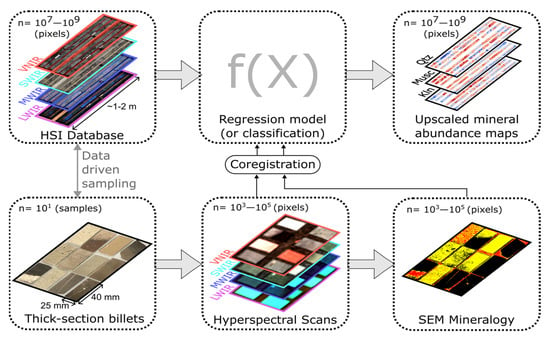
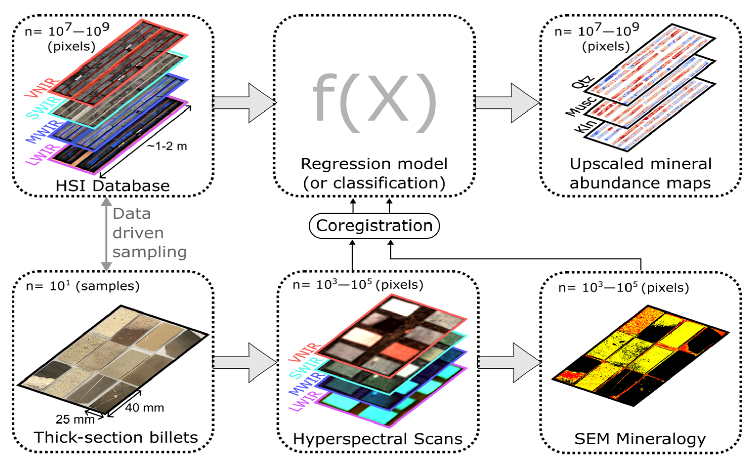
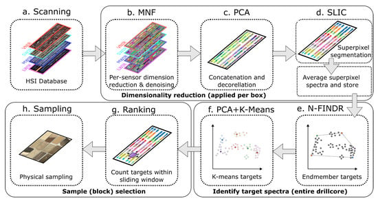
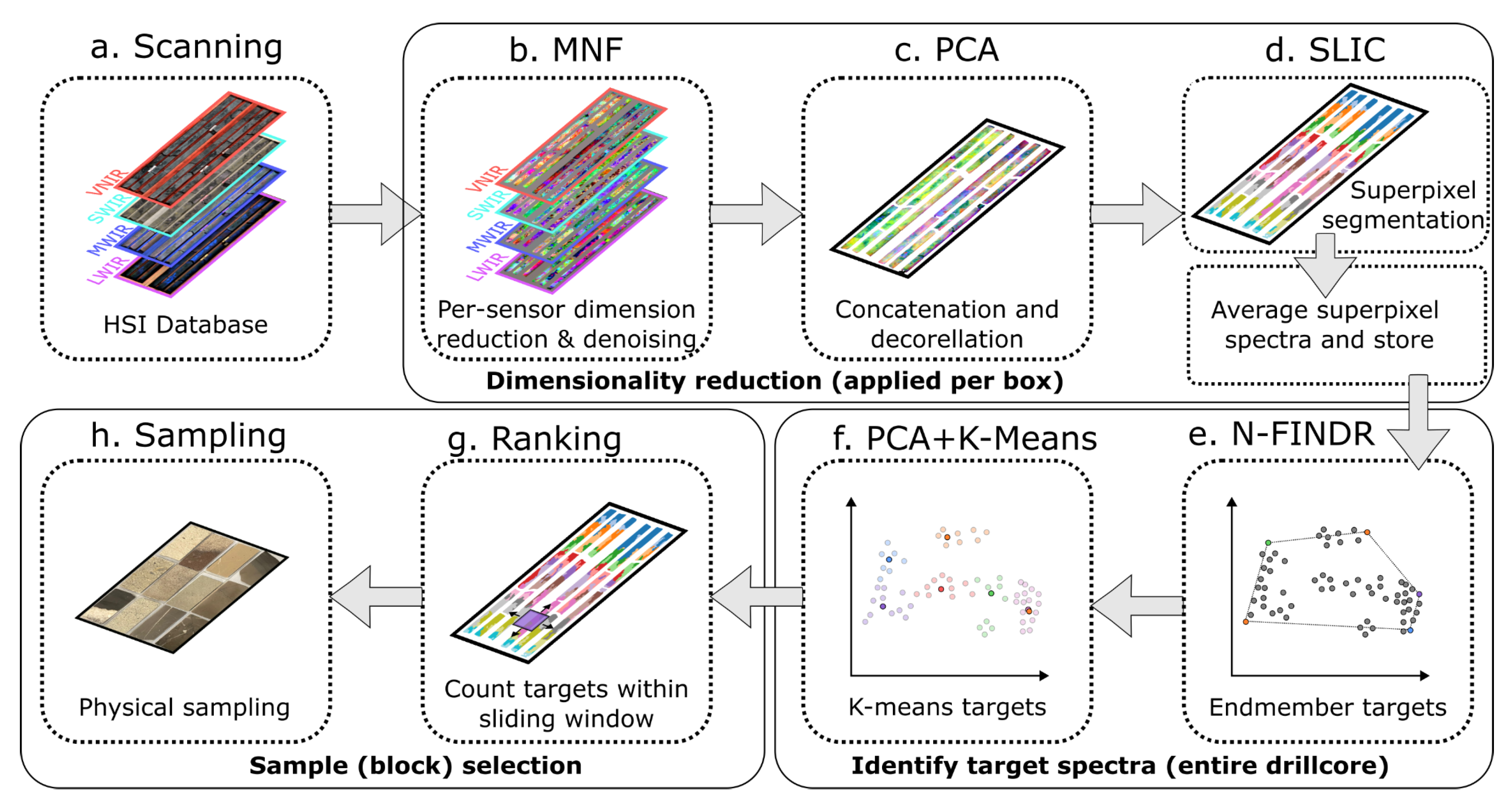
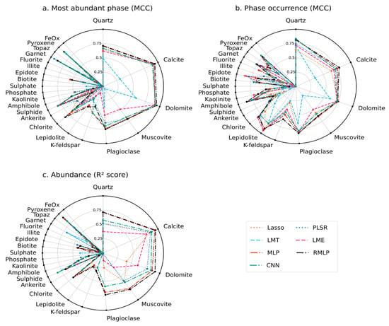
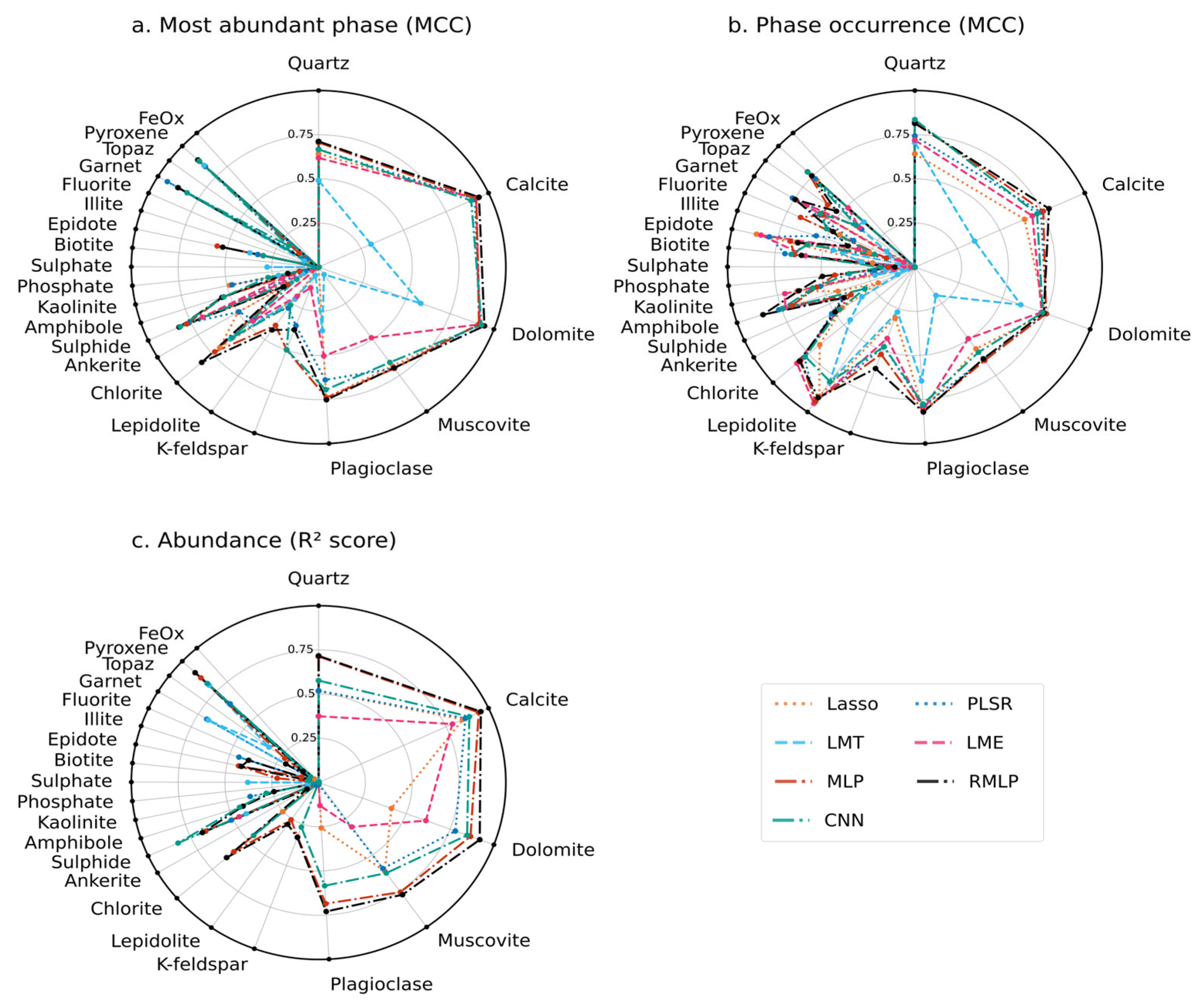
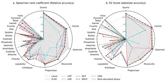
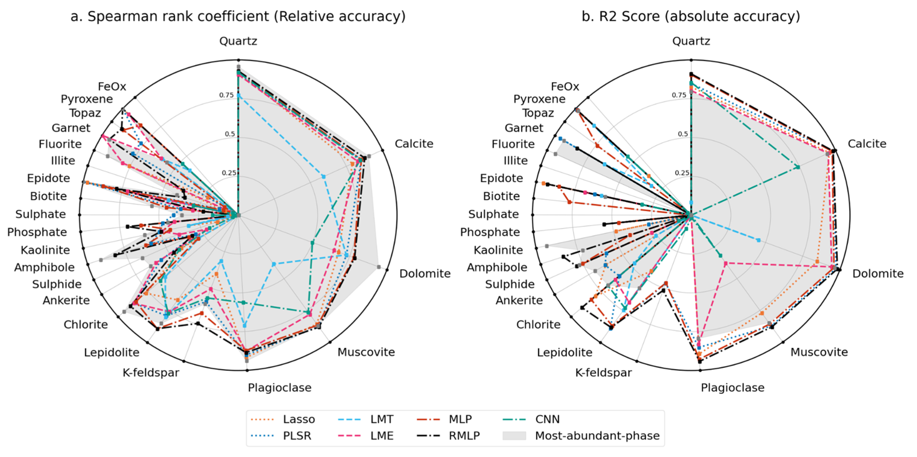
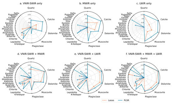
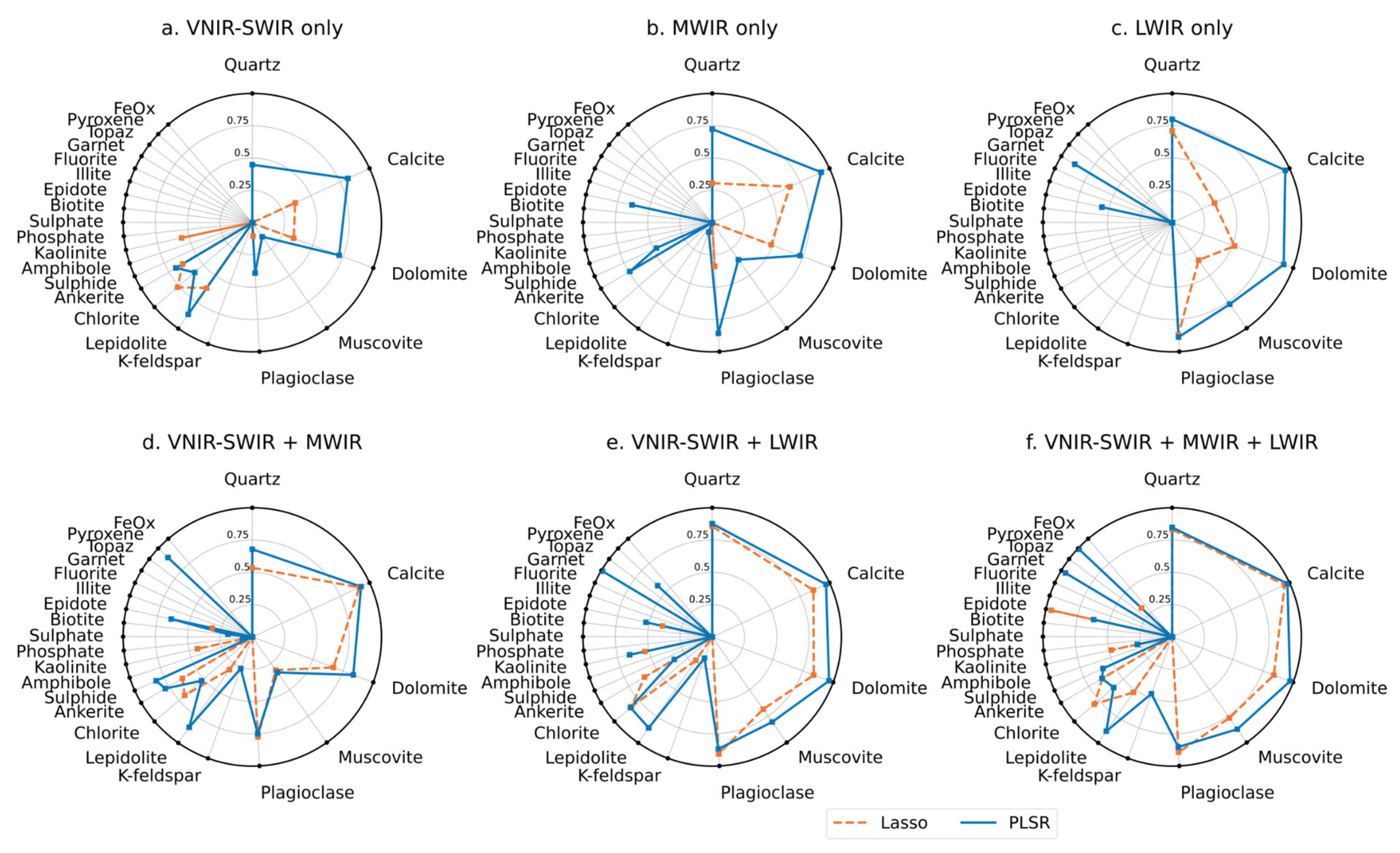
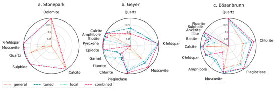
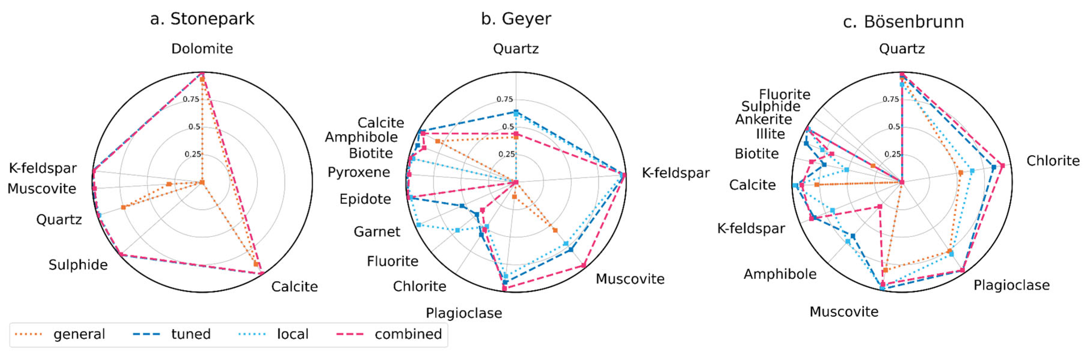
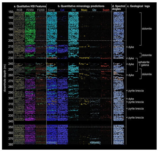
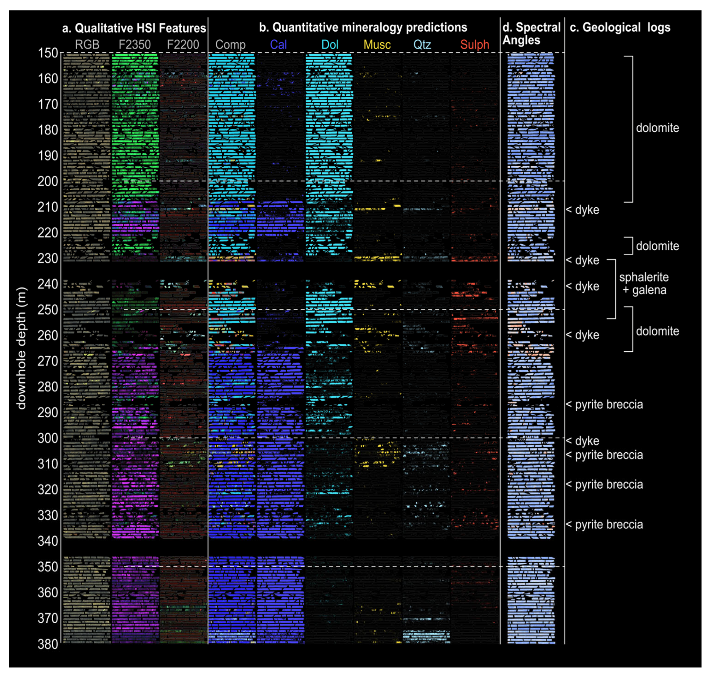
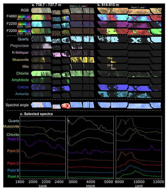
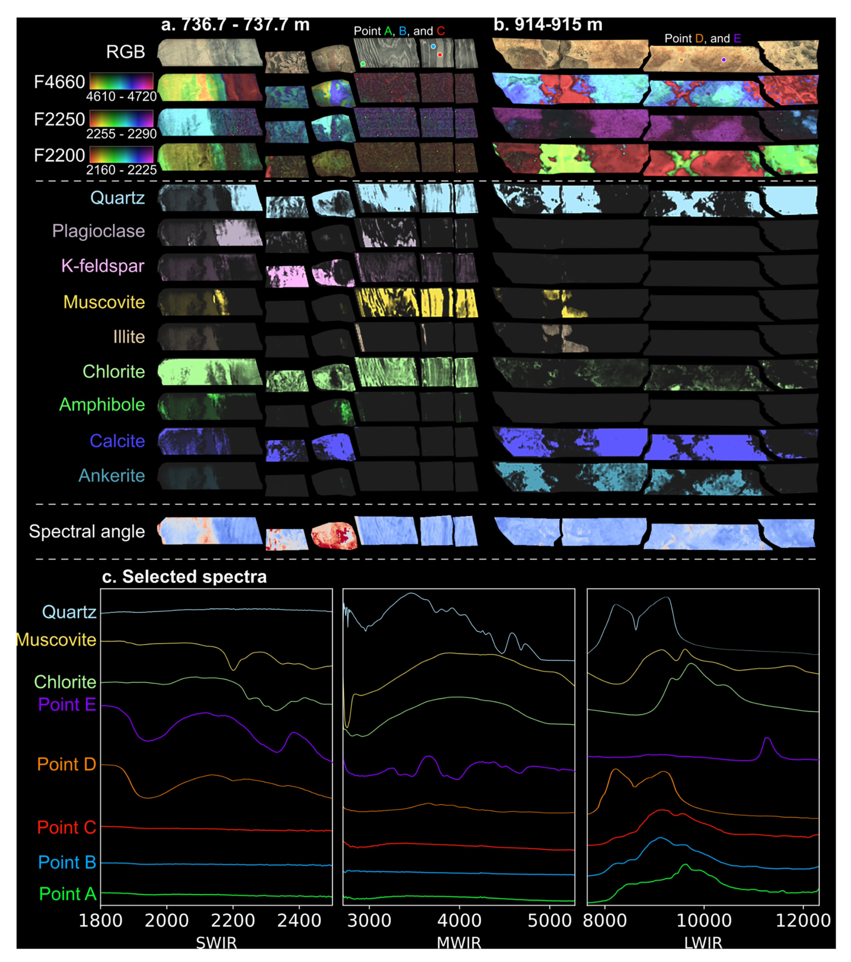
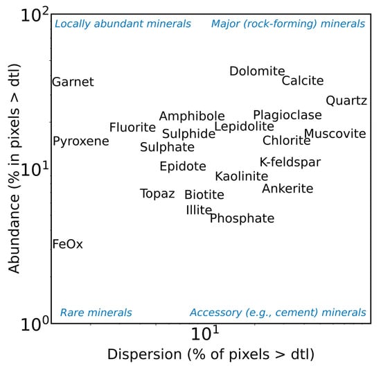

Disclaimer/Publisher’s Note: The statements, opinions and data contained in all publications are solely those of the individual author(s) and contributor(s) and not of MDPI and/or the editor(s). MDPI and/or the editor(s) disclaim responsibility for any injury to people or property resulting from any ideas, methods, instructions or products referred to in the content. |
© 2026 by the authors. Licensee MDPI, Basel, Switzerland. This article is an open access article distributed under the terms and conditions of the Creative Commons Attribution (CC BY) license.