Delineation of Concealed Copper–Cobalt Mineralization Targets Using Semi-Airborne Transient Electromagnetic Data in the Kambove Mining District, Democratic Republic of the Congo

Abstract

As supply risks for cobalt and other critical metals increase, detecting concealed orebodies in mature mining districts has become increasingly important for resource renewal. The Ksignal area, located on the margin of the Kambove mining district in the Democratic Republic of the Congo, lies near the M’sesa-Shangolowe structural system and exhibits copper geochemical anomalies. Together with the district’s position in the core of the Central African Copperbelt, these features indicate strong potential for concealed copper–cobalt mineralization. To investigate this potential, we conducted a semi-airborne transient electromagnetic survey in the Ksignal area. Because induced polarization effects can distort transient electromagnetic responses and complicate resistivity interpretation, we account for these effects and jointly estimate resistivity and chargeability from the observed data. The resulting resistivity–chargeability framework reveals an electrical discontinuity, which we interpret as an electrical structural interface in the Ksignal area. By integrating this inferred interface with borehole constraints and copper geochemical anomalies, we identify and interpret composite anomalies related to concealed mineralization. The results delineate a coherent candidate zone east of the inferred electrical structural interface, trending from near north–south to north-northwest and partly coinciding with the copper geochemical anomaly. This work provides geophysical evidence for deep and peripheral exploration in the Kambove mining district and supports the development of multiparameter target-delineation workflows for brownfield exploration.

1. Introduction

The global transition towards low-carbon and electrified energy systems is intensifying concerns over the supply security of critical metals such as cobalt [1,2]. Cobalt is an important component of cathode materials in high-energy-density lithium-ion batteries. It is closely linked to battery thermal stability, cycle life and safety, giving it strategic importance in the new-energy supply chain [3]. The Central African Copperbelt (CACB) is one of the world’s most important sediment-hosted copper–cobalt metallogenic provinces and a core region for global cobalt supply [4,5,6]. It hosts numerous stratabound, stratiform and structurally modified copper–cobalt deposits, and long-term mining has formed several mature mining districts [7,8,9,10]. As shallow resources that are easy to identify and mine become depleted, detecting deep and peripheral concealed orebodies in the CACB and its mature mining districts is important for improving cobalt resource replacement and supporting sustained mine development [11,12].

Electromagnetic methods can image subsurface structure by exploiting electrical contrasts among orebodies, host rocks and structural zones, making them important tools for deep exploration of metallic deposits [13,14,15,16]. Conventional ground-based controlled source electromagnetic methods are sensitive to conductive targets, but receiver deployment is often constrained in areas with complex surface conditions. Open pits, water bodies, roads, industrial buildings, vegetation and rugged topography can prevent continuous and high-density observation coverage [17,18]. Conventional airborne electromagnetic methods offer high operational efficiency and broad regional coverage. However, for small-scale, low-volume and high-precision exploration in and around mining districts, they can be costly per line kilometre and less flexible in flight planning, site coordination and operational windows [19]. The semi-airborne transient electromagnetic method (SATEM) deploys a high-power transmitter on the ground and carries a lightweight receiver on an unmanned aerial vehicle (UAV) or other airborne platform, combining strong-source transmission with rapid mobile acquisition [18,20,21,22,23,24,25]. This configuration combines the deep-probing capability of a ground-based source with the high-density sampling advantage of low-altitude flight, providing a more adaptable technical approach for deep and peripheral exploration in mining districts [26,27,28].

Copper–cobalt mineralized bodies can exhibit induced polarization (IP) responses because metallic minerals and associated sulphides promote charge accumulation and relaxation at mineral-grain, pore-fluid and solid–liquid interfaces [29,30]. This effect is particularly useful for identifying disseminated and veinlet mineralization. In time-domain electromagnetic data, IP effects modify the post-turn-off decay curve, commonly producing slower late-time decay, curve distortion and, in some cases, sign reversal [31,32,33]. If these effects are ignored, SATEM inversion based only on a non-polarizable resistivity model may bias the inferred resistivity structure, anomaly boundaries and target geometry. SATEM interpretation for copper–cobalt mineralization should therefore not rely solely on resistivity. Instead, resistivity and chargeability should be jointly extracted to better distinguish conductive anomalies, polarization-related anomalies and their possible geological causes.

This study focuses on the Ksignal area in the Kambove mining district, Democratic Republic of the Congo. The area lies on the margin of the Kambove district, close to the M’sesa-Shangolowe structural system, and contains copper geochemical anomalies, indicating potential for concealed copper–cobalt mineralization. To address the challenges of complex surface conditions, restricted ground-based receiver deployment and deep peripheral exploration, we conducted UAV-based SATEM surveys in the Ksignal area. Using the SATEM data, we first established the subsurface resistivity–chargeability framework and identified an electrical discontinuity that is interpreted as an electrical structural interface. We then integrated this inferred interface with copper geochemical anomalies and borehole constraints to evaluate composite anomalies and delineate a candidate concealed copper–cobalt mineralized zone. This integrated workflow delineates a candidate concealed mineralized zone in the Ksignal area and provides a reproducible strategy for interpreting SATEM multiparameter data in deep and peripheral exploration around the Kambove mining district.

2. Materials and Methods

2.1. Geological Setting

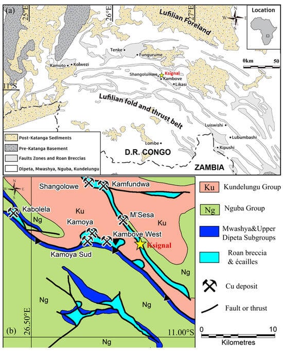
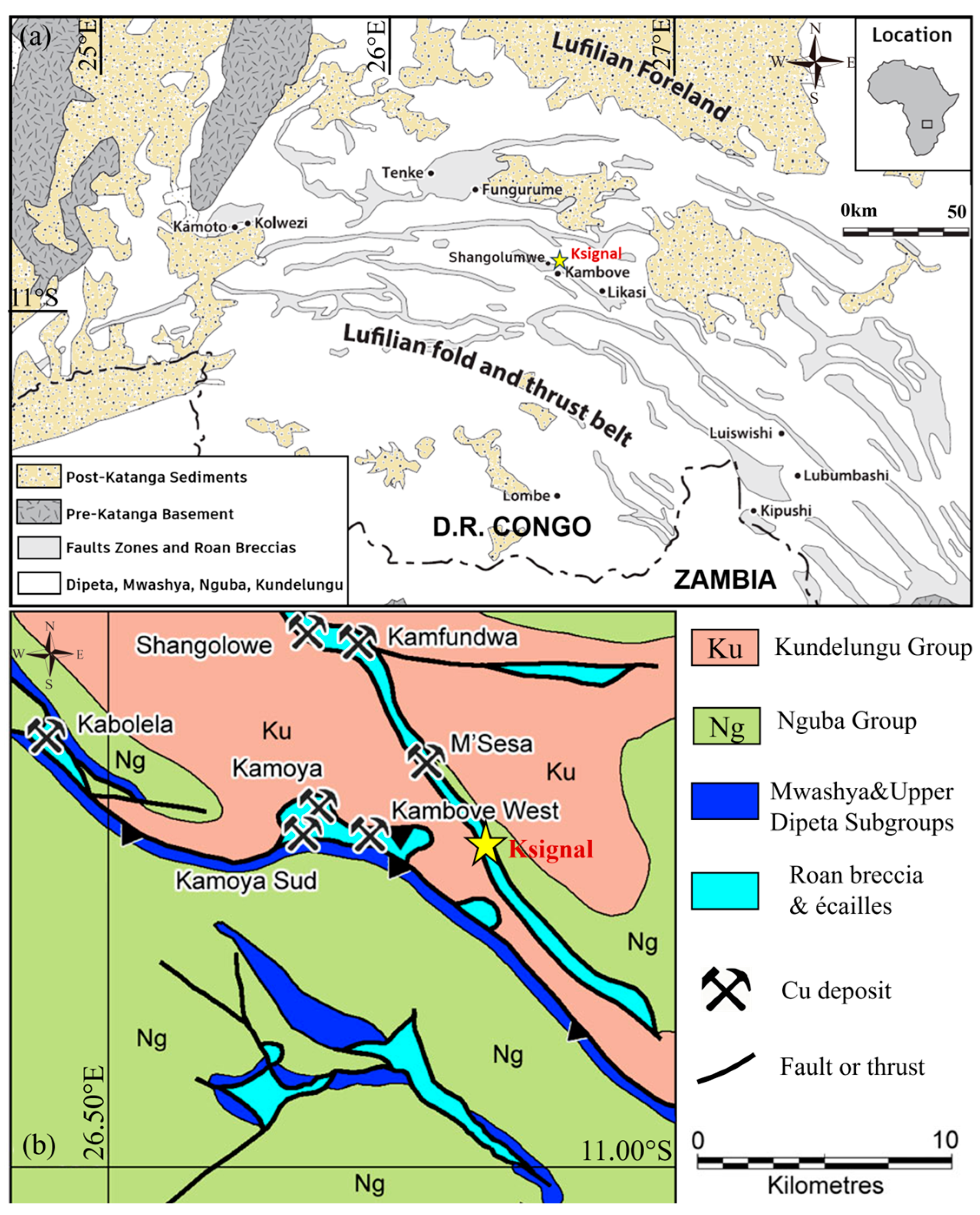
The Central African Copperbelt (CACB) extends across northern Zambia and southern Democratic Republic of the Congo. It is one of the world’s major sediment-hosted copper–cobalt metallogenic provinces and a core region for global cobalt supply [4]. As shown in Figure 1a, the belt developed within the Neoproterozoic Katanga Basin. Its formation is closely linked to rift-related sedimentation during the breakup of Rodinia and subsequent Lufilian orogenesis [34,35]. The Katanga Supergroup is commonly divided into the Roan, Nguba and Kundelungu groups. Of these, the Roan Group, especially the Mines Subgroup, hosts the most concentrated copper–cobalt mineralization [6,36]. Assemblages of reduced carbonate rocks, shale, dolomite and siliceous rocks provided favourable redox interfaces and storage space for copper–cobalt precipitation [37].

Figure 1. Regional and local geological setting of the Ksignal survey area in the Kambove mining district. (a) Regional tectonic framework of southeastern Democratic Republic of the Congo, showing the location of the Ksignal survey area within the Lufilian fold-and-thrust belt. (b) Simplified geological map of the Kambove–Shangolowe area, showing the local geological context and the location of the Ksignal survey area. (Modified after Refs. [38,39]).

Copper–cobalt mineralization in the CACB is jointly controlled by sedimentary architecture, basin-fluid migration and later structural modification [40]. Metal-rich oxidized basin brines migrated along faults, permeable strata and structurally weakened zones. When these fluids encountered organic-rich rocks, sulphides or reduced carbonate rocks, metal precipitation produced stratabound or stratiform copper–cobalt mineralization [41]. Lufilian orogenesis subsequently folded, thrusted and inverted the original sedimentary basin, locally transforming mineralized horizons into tectonic slices, breccia bodies or lenticular orebodies [42]. Mineralization interpretation in the study area must therefore consider the superposition of stratigraphic and structural controls [43].

The Kambove mining district lies in the core of the Congolese segment of the CACB. As shown in Figure 1b, it contains several deposits and mineralized occurrences, including Kambove, Kambove West, Kamoya, Kabolela, Kamfundwa, Shangolowe and M’sesa. The district is controlled by the Kambove anticline, the M’sesa-Shangolowe structural zone and associated subsidiary faults. Breccia windows, tectonic slices, thrust-nappe interfaces and strike-slip shear zones are locally developed [42]. Known copper–cobalt orebodies are commonly associated with mineralized horizons of the Roan Group, structurally fractured zones and breccia systems. Their morphologies include tabular, lenticular, banded and irregular tectonic-slice forms [42,44].

As shallow oxidized ore resources are progressively depleted, deep primary sulphide orebodies, concealed orebodies near structural interfaces and peripheral anomaly zones have become important targets for resource replacement in the district. The Ksignal area lies on the margin of the Kambove district, close to the M’sesa-Shangolowe structural system and areas where breccias and tectonic slices are developed. The area also shows pronounced copper enrichment anomalies. These geological and geochemical features indicate potential for concealed copper–cobalt mineralization.

2.2. Data Acquisition

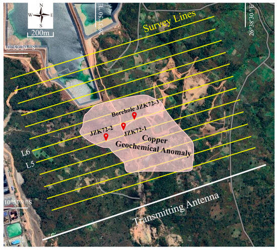
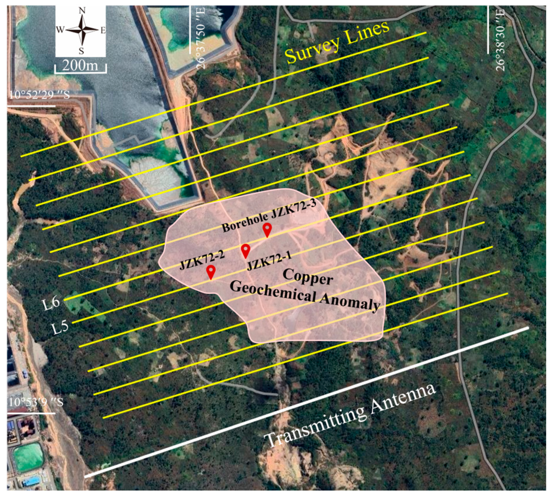
The Ksignal area was surveyed using a UAV-based SATEM configuration with a grounded transmitter and a single-coil airborne receiver. As shown in Figure 2, the survey lines covered the main copper geochemical anomaly and its surrounding area, and were arranged approximately parallel to the ground transmitting wire.

Figure 2. Satellite image and survey layout of the Ksignal area. The yellow parallel lines indicate the UAV-based semi-airborne transient electromagnetic survey lines, while the white line marks the position of the grounded transmitting antenna. Red location markers denote the boreholes used for geological control, and the shaded area outlines the projected extent of the known copper geochemical anomaly.

Dense survey lines crossed the main anomaly zone, allowing the geometry, burial depth and continuity of resistivity and polarization responses to be compared across different profiles. This layout was designed to establish the spatial variation in electrical anomalies through multiple near-parallel lines, thereby constraining subsequent prediction of concealed mineralized bodies.

The distance between the two grounding electrodes was approximately 2 km. The transmitter delivered a bipolar square-wave current with a base frequency of 25 Hz through the grounded wire, with a current amplitude of 25 ± 0.2 A. Receiver lines were deployed north of the transmitting wire. A total of 12 lines were acquired, each approximately parallel to the transmitting wire. Each line was about 1700 m long, with a line spacing of 100 m and a minimum transmitter-receiver offset of about 200 m.

The receiving system consisted of a lightweight receiver and a vertical induction-coil sensor. The receiver used a 32-bit ADC with a sampling rate of 100 kHz, consumed approximately 3.4 W, weighed about 620 g and could operate continuously for nearly 10 h on a single charge. The transmitter and receiver were synchronized using GPS-disciplined oven-controlled crystal oscillators, with a synchronization accuracy of about 100 ns. The vertical induction-coil sensor had a resonant frequency of 52 kHz, a noise level of approximately 0.1 nT/s and a total weight of about 2.29 kg.

Because the UAV motors and airframe can generate electromagnetic interference, the induction-coil sensor was not rigidly mounted directly beneath the aircraft. Instead, it was suspended below the UAV using a flexible connection to reduce platform-related electromagnetic noise in the recorded signal. Suspended deployment can introduce motion noise caused by air resistance and attitude variations. This problem can be amplified during terrain-following flight in areas with pronounced topographic relief, where sensor motion becomes more complex and both the amplitude and frequency bandwidth of motion noise may increase. These effects can increase the difficulty of subsequent data processing.

We therefore used constant-altitude flight to keep the sensor motion relatively stable. Because this flight mode causes the sensor ground clearance to vary among measurement points, the survey area was first reconstructed in three dimensions using a small aerial-photography UAV. Surface elevation was then extracted at each measurement point. The actual sensor ground clearance was calculated as the difference between the sensor GPS elevation and the corresponding surface elevation, and was used as an auxiliary parameter in subsequent data processing and inversion interpretation.

2.3. Data Processing and Inversion

UAV-based SATEM observations must be converted from raw time series into windowed decay curves for inversion, and processing quality directly affects interpretation of deep electrical structure. The raw data from the Ksignal area may be affected by sferic pulses, power-line and industrial background noise, motion-induced noise from the UAV platform, and swing or attitude changes in the suspended sensor. Motion-induced noise and low-frequency drift are especially pronounced at late-time gates, where the response is closely related to deeper subsurface information. Data processing must therefore suppress non-geological noise while preserving the continuity and physical form of the transient decay curves, so that real deep anomalies are not oversmoothed or weakened.

Conventional processing workflows usually address different noise types with separate procedures, including removal of abnormal segments, stacking and averaging, filtering, motion-noise correction and channel-by-channel quality control. These methods have clear physical meaning, but involve multiple processing steps, and their parameter choices often depend strongly on operator experience. To improve workflow consistency and automation, we used a denoising autoencoder (DAE) to suppress multi-source noise in the raw time series.

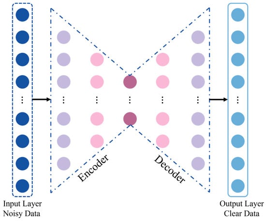
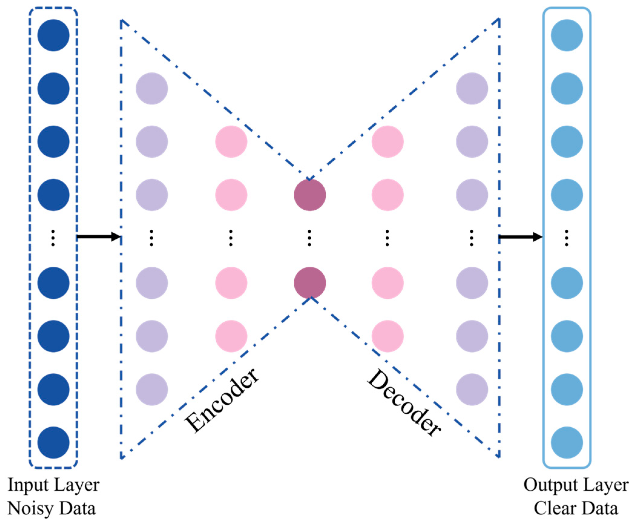
The DAE architecture used in this study is shown in Figure 3. Both the input and output layers contain 1000 sampling points, corresponding to a 10 ms observation window at a sampling rate of 100 kHz. The encoder and decoder each consist of four layers, and the final latent layer contains 100 nodes. ReLU was used as the activation function, and mean squared error (MSE) was used as the loss function. The encoder extracts the main features of the time series, and the decoder reconstructs the denoised curve. Compared with conventional noise-specific processing, this approach suppresses multi-source noise within a unified data-driven framework while preserving response morphology related to subsurface electrical structure.

Figure 3. Schematic architecture of the denoising autoencoder used for transient electromagnetic data processing.

The DAE training dataset was constructed by combining synthetic SATEM responses with measured environmental noise. To enhance the generalization capability of the DAE, the synthetic training dataset was constructed using three-, four-, and five-layer geoelectric models covering a broad range of electrical and polarization properties. Layer resistivities were sampled at logarithmically equal intervals between 10¹~10⁴ Ω∙m, and the layer interfaces were distributed within a depth range of 0–1500 m. Chargeability values were then randomly assigned according to the resistivity of each layer. For layers with resistivities lower than 10² Ω∙m, chargeability was randomly selected between 65% and 100%. For resistivities ranging from 10²~10³ Ω∙m, chargeability was selected between 35% and 70%, whereas values between 0% and 40% were assigned to layers with resistivities ranging from 10³~10⁴ Ω∙m. This parameterization allowed the training dataset to include conductive and strongly polarizable media, moderately polarizable formations, and relatively resistive backgrounds with weak polarization responses. Measured noise was obtained from pure-noise flights conducted with the transmitter switched off [45]. The noise records were superimposed on the synthetic responses to form the network input data, while the corresponding noise-free synthetic responses were used as the target outputs. Because transient electromagnetic decay curves have a large dynamic range, amplitude compression was applied before network input to reduce the contrast between strong early-time signals and weak late-time signals. The corresponding inverse transformation was then applied to the network output to recover decay curves in their original physical units. For the independent synthetic test data, the relative differences between the DAE outputs and the corresponding noise-free theoretical responses were generally less than 2%. Detailed descriptions of the network architecture, training strategy, signal-to-noise-ratio evaluation, and model-validation procedure have been reported in our previous study [46].

To improve the applicability of the network to the Ksignal survey, additional pure-noise flight data were collected in the study area and incorporated into the training dataset. Synthetic models representing the resistivity, chargeability, and burial-depth ranges inferred from the available geological information were also added, after which the network was retrained. These procedures were intended to reduce the risk that incomplete noise characteristics or inadequate geological representation in the training dataset would cause attenuation or distortion of valid geological signals.

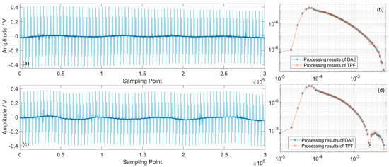
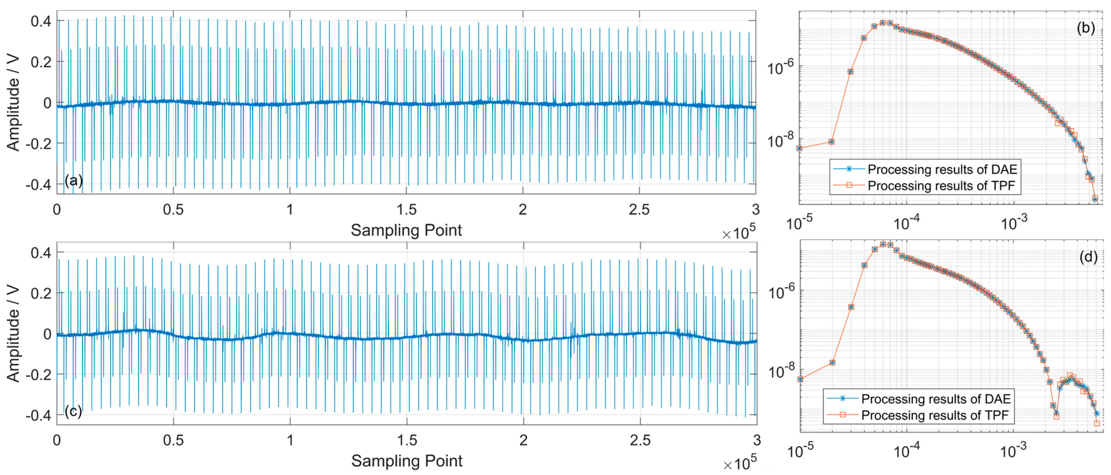
The performance of the DAE on the field data was evaluated by comparison with the traditional processing flow (TPF), as shown in Figure 4. For both conventional decay responses and responses containing observable induced polarization effects, the two methods preserve similar overall decay characteristics. Between 1 × 10⁻⁴~2 × 10⁻³ s, the mean relative difference between the DAE and TPF results is less than 1%. At later times, the mean difference increases to approximately 5%, mainly because of the lower signal-to-noise ratio, whereas the DAE results exhibit better continuity between adjacent time channels and measurement stations. These comparisons indicate that the network does not simply attenuate anomalous curves. Instead, it improves late-time data quality while retaining the main decay characteristics, providing a more stable data basis for subsequent multiparameter inversion.

Figure 4. Comparison of representative transient electromagnetic records and the corresponding denoised decay curves. Panels (a,c) show two raw time-series records. Panels (b,d) compare the decay curves recovered using the denoising autoencoder (DAE) and the traditional processing flow (TPF). The close agreement between the two processing results indicates that the DAE preserves the principal transient-response characteristics during noise suppression. Compared with (b), the decay curve in (d) exhibits a more pronounced late-time sign reversal, indicating a stronger induced-polarization response.

Copper–cobalt mineralized bodies commonly have strong electronic conductivity and can generate interfacial polarization. In time-domain electromagnetic responses, induced polarization effects modify the decay of the secondary field after current turn-off. These effects appear as slower late-time decay, curve distortion and, in some cases, local sign reversal. If the subsurface is simplified as a non-polarizable medium during inversion, the inferred position, scale and amplitude of resistivity anomalies may be biased [31,32]. To characterize both electromagnetic induction and polarization responses, we used the Cole–Cole complex resistivity model to describe the dispersive behaviour of subsurface media:

$$\sigma \left(\omega \right)= {\sigma }_{\infty } \left[1 - {\displaystyle \frac{\eta }{1 +{\left(i\omega \tau \right)}^c }}\right]$$

(1)

where $\sigma \left(\omega \right)$ is the complex conductivity, ${\sigma }_{\mathrm{\infty }}$ is the high-frequency conductivity, $\eta$ is the polarization parameter (chargeability), $\tau$ is the time constant, $c$ is the frequency-dependence coefficient, $\mathsf{\omega }$ is the angular frequency, and $i$ is the imaginary unit. This model provides the physical basis for jointly extracting resistivity and polarization parameters from UAV-based SATEM data.

Because of late-time signal-to-noise limitations and differences in parameter sensitivity, it is usually difficult to stably invert resistivity, chargeability, time constants and frequency-dependence coefficients simultaneously. To reduce the non-uniqueness associated with the four-parameter Cole–Cole inversion, the time constant ($\tau$) and frequency-dependence coefficient (c) were fixed, whereas resistivity and chargeability were treated as the principal inversion parameters [47]. The time constant was estimated from the observed SATEM decay curves. A total of 150 stations were randomly selected from the subset of measurement points exhibiting clear induced polarization effects. The decay curves at these stations were decomposed in the $\tau$ domain [48]. For each station, the relative contribution of each time-constant component was calculated, and components with contributions greater than 10% were retained as statistically significant [49]. The resulting time constants were primarily distributed between 1 × 10⁻³~1 × 10⁻² s. Within this interval, the value occurring at the largest number of stations was 5 × 10⁻³ s; therefore, τ was fixed at 5 × 10⁻³ s in the subsequent inversion. The frequency-dependence coefficient was fixed at 0.5. This value corresponds approximately to a Warburg-type response and is commonly considered representative of induced polarization associated with disseminated metallic minerals [30]. A synthetic sensitivity analysis was subsequently performed to evaluate the influence of the selected τ and $c$ values on the recovered resistivity and chargeability. With all other parameters held constant, $\tau$ was varied from 3 × 10⁻³~7 × 10⁻³ s, whereas c was varied from 0.4 to 0.6. Within the tested ranges, the errors were less than 0.6% for variations in $\tau$ and less than 0.5% for variations in $c$. These results indicate that the recovered resistivity and chargeability are only weakly affected by moderate variations in the fixed Cole–Cole parameters under the present survey configuration and geological model. Therefore, fixing $\tau$ at 5 × 10⁻³ s and c at 0.5 provides a reasonable simplification that improves inversion stability while preserving the principal resistivity and chargeability characteristics relevant to geological interpretation.

The model parameters can be expressed as:

$$m={[{\rho }_1,{\rho }_2,\cdots ,{\rho }_N,{\eta }_1,{\eta }_2,\cdots ,{\eta }_N]}^T,$$

(2)

where ${\rho }_N$ and ${\eta }_N$ are the resistivity and chargeability of the $N$-th layer, respectively, and $N$ is the number of layers. The subsurface model was parameterized as a one-dimensional layered-earth model at each measurement station. The thicknesses of the model layers were prescribed before inversion and remained fixed throughout the optimization. The thickness of the first layer was set to 10 m, and the thickness of each subsequent layer was increased geometrically by a factor of 1.06. This discretization provides relatively fine resolution in the shallow subsurface, where early-time electromagnetic data contain greater high-frequency information, while progressively increasing the layer thickness at depth to account for the decreasing vertical resolution caused by diffusive attenuation of the electromagnetic field. A total of 35 layers were used, extending the inversion model to a depth of approximately 1.2 km. Because the layer geometry was fixed, only the electrical parameters of the individual layers were updated during inversion. The initial resistivity model was assigned a uniform value of 500 Ω∙m. The initial chargeability model was selected according to the characteristics of the observed decay curve. For stations exhibiting directly identifiable induced polarization effects, the initial chargeability was set to 0.8, whereas a lower initial value of 0.2 was used for stations without an evident induced polarization response. The Cole–Cole time constant and frequency-dependence coefficient were fixed at 5 × 10⁻³ s and 0.5, respectively, and only resistivity and chargeability were updated during inversion.

The inversion objective function consists of a data misfit term and a model regularization term:

$$\mathsf{\Phi }\left(m\right)={\left|\right|W_d\left[F\right(m) - d_{obs}]\left|\right|}_2^2+{\alpha \left|\right|W_{m}m\left|\right|}_2^2$$

(3)

where $d_{obs}$ is the observed decay curve, $F\left(m\right)$ is the forward response, $W_d$ is the data-weighting matrix, $W_m$ is the model-constraint matrix, and $\alpha$ is the regularization parameter. Data weights were assigned according to noise level, time-gate stability and curve quality to reduce the influence of anomalous noisy gates on the inversion. The model-constraint term suppresses unrealistic oscillations between adjacent layers, allowing the inversion to fit the data while maintaining the required vertical stability.

The inversion was terminated when either the maximum number of 15 iterations was reached, or the relative RMS fitting error decreased to 5% or less. If the inversion terminated with a relative RMS error greater than 10%, the initial resistivity and chargeability models were adjusted, and the inversion was repeated. Only inversion results with relative RMS errors of 10% or less were retained for subsequent interpretation. These settings were adopted to balance data fitting, inversion stability, and computational efficiency.

3. Results

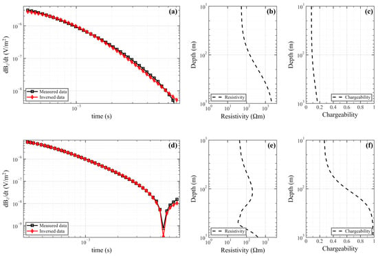
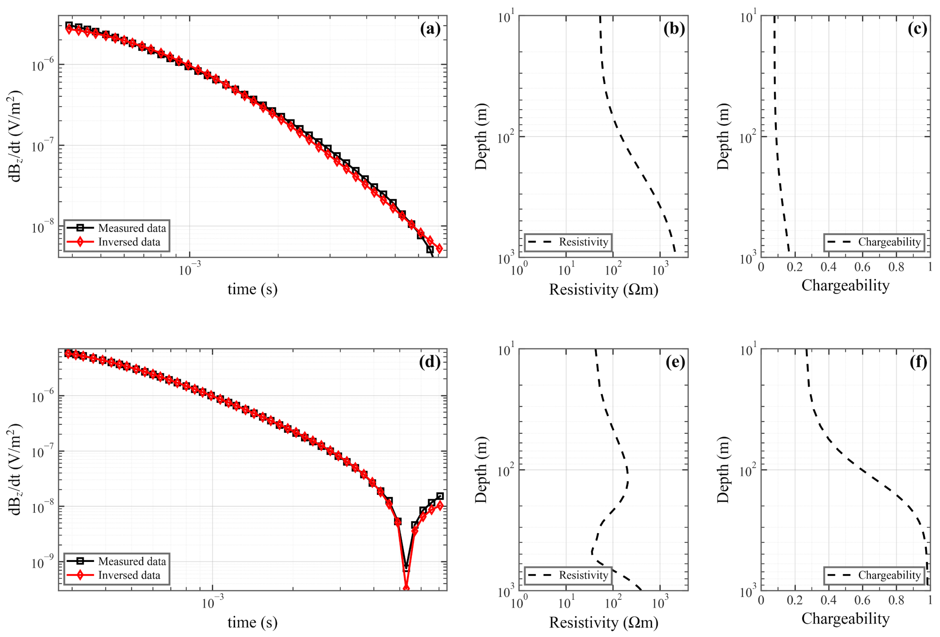
To quantitatively evaluate the performance of the data-processing and inversion workflow, two representative stations were selected for detailed analysis, as shown in Figure 5. The two stations are characterized by a conventional transient electromagnetic decay response and a decay response strongly affected by induced polarization, respectively. The relative fitting errors of the two stations are approximately 10% and 5%, respectively. At the station exhibiting a conventional electromagnetic response, the observed decay curve is generally smooth and continuous, without pronounced late-time distortion. The inversion recovers a relatively stable resistivity structure and a low-chargeability background. At the station exhibiting a pronounced induced polarization response, the late-time channels are characterized by a slower decay rate and localized anomalous variations. The inversion recovers a distinct high-chargeability layer while maintaining good agreement between the predicted and observed decay curves. These results indicate that the decay curves obtained after data processing retain the principal information required for inversion. They also support the ability of the joint resistivity–chargeability inversion to reproduce both conventional electromagnetic induction responses and responses containing substantial induced polarization effects.

Figure 5. Inversion results for two representative stations. Panels (a–c) show a station characterized by a conventional transient electromagnetic decay response, including the measured and predicted decay curves (a), inverted resistivity model (b), and inverted chargeability model (c). Panels (d–f) show a station with a pronounced induced-polarization response, including the measured and predicted decay curves (d), inverted resistivity model (e), and inverted chargeability model (f).

The inversion results also show that resistivity and chargeability differ in their sensitivity to subsurface anomalies. Resistivity mainly reflects conductive structures, stratigraphic contacts and the geometric boundaries of anomalous bodies. Chargeability is more sensitive to media with strong interfacial polarization. Because chargeability may provide weaker constraints on the lower boundaries of deep anomalous bodies than resistivity, subsequent interpretation used resistivity structure to constrain anomaly geometry and chargeability to assist in evaluating anomaly properties.

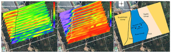
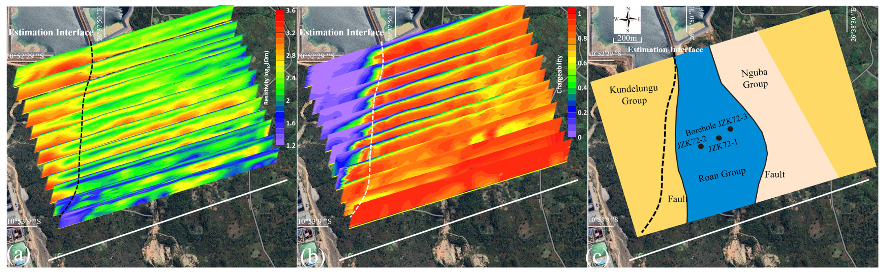
Based on the inversion-quality assessment, the resistivity and chargeability sections from all survey lines were projected onto the satellite image according to their actual spatial coordinates to examine the lateral continuity and spatial distribution of the anomalies, as shown in Figure 6. The resistivity sections exhibit generally good continuity between adjacent survey lines. The electrical anomalies are not restricted to isolated positions along individual lines but form relatively consistent spatial zones across the survey area. A pronounced electrical discontinuity, trending approximately north–south to north-northwest, can be identified from the western to central part of the survey area and traced across multiple survey lines. The chargeability sections further emphasize this boundary. The area west of the inferred interface is dominated by relatively low chargeability, whereas moderate-to-high chargeability responses are widely distributed to the east. The spatial coincidence of the resistivity discontinuity and the chargeability contrast indicates a systematic lateral change in subsurface electrical and polarization properties.

Figure 6. Spatial projection of the inversion results and corresponding geological interpretation in the Ksignal survey area. (a) Inverted resistivity sections. (b) Inverted chargeability sections. The dashed line indicates the estimated interface separating the relatively resistive and weakly polarizable western domain from the relatively conductive and highly polarizable eastern domain. (c) Simplified geological map showing the distribution of the Kundelungu, Roan, and Nguba groups, the fault structures, and the locations of boreholes JZKT2-1, JZKT2-2, and JZKT2-3.

To provide independent geological evidence for this interpretation, a simplified geological map covering the survey area was reconstructed from the geological map supplied by the mining company and compared with the geophysical results. As shown in Figure 6c, the central part of the survey area is mainly occupied by the Roan Group, which is bounded by the Kundelungu Group to the west and the Nguba Group to the east. Several mapped faults occur along or near these lithological boundaries. The inferred geophysical interface broadly follows the north–south to north-northwest structural trend shown on the geological map and is spatially close to the mapped western boundary of the Roan Group. The general agreement in orientation and regional position supports the interpretation that the electrical discontinuity is related to a major lithological or structural boundary rather than to an isolated geophysical anomaly. A local offset remains between the inferred electrical interface and the mapped geological boundary, particularly in the southern part of the survey area closer to the transmitter. The local discrepancy between the inferred geophysical interface and the mapped geological boundary may be attributed to two main factors. First, the geophysical interface represents the position of the strongest subsurface electrical contrast rather than the surface trace of the geological boundary. If the stratigraphic contact or fault is inclined, its geophysical expression at depth may be laterally displaced relative to its surface outcrop. Second, in the very short-offset region close to the transmitter, source-related three-dimensional effects become pronounced, and the electromagnetic field cannot be adequately represented by a one-dimensional layered-earth approximation.

Therefore, the inferred interface should not be regarded as an exact reproduction of the mapped geological contact. Instead, it represents a subsurface electrical boundary that is broadly consistent with the mapped structural and lithological framework. The combined resistivity and chargeability results suggest that the two sides of the interface differ in lithological composition, fracture development, groundwater conditions, alteration, or mineralization-related polarization properties. In the geological context of the Kambove district, the interface is interpreted as part of the fault- and stratigraphy-controlled structural framework associated with the Roan Group. Such boundaries may influence the migration, alteration, and spatial concentration of copper–cobalt mineralization.

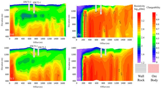
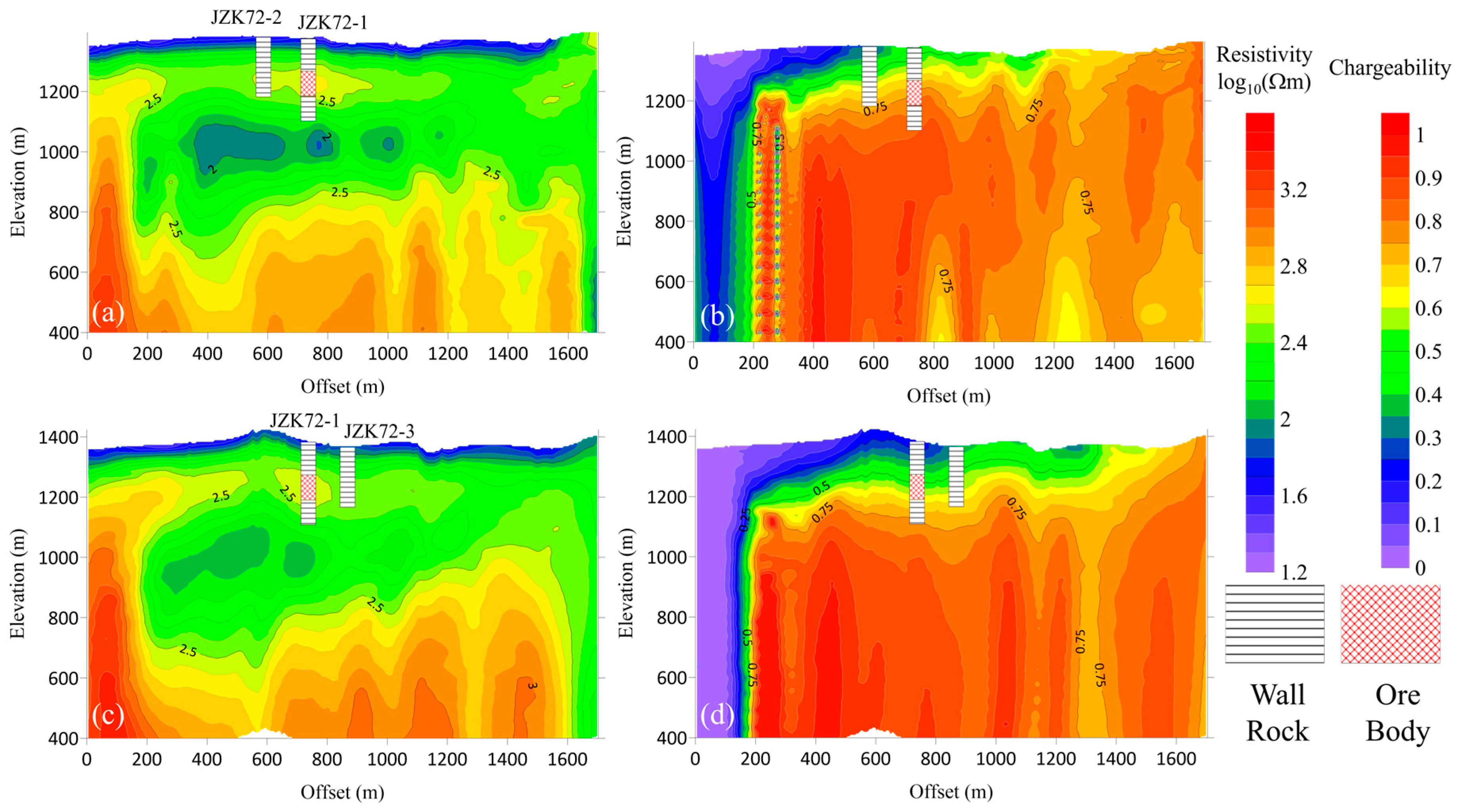
After establishing the survey-wide electrical framework, we selected the borehole-constrained L5 and L6 survey lines for detailed interpretation, with the aim of linking geophysical anomalies to known mineralization. Borehole data provide local calibration for assigning geological meaning to resistivity and chargeability anomalies. As shown in Figure 7, the intersected mineralized intervals do not simply coincide with the lowest-resistivity zones. Instead, they occur mainly within a relatively stable moderate-to-high resistivity background and are commonly associated with medium-to-high chargeability responses. This pattern indicates that chargeability is a useful indicator of mineralization-related properties. By contrast, low-resistivity anomalies without simultaneous chargeability enhancement are more likely to reflect water-bearing fractured zones, shallow conductive media or other non-mineral factors.

Figure 7. Inversion sections and borehole constraints for survey lines L5 and L6. Panels (a,b) show the inverted resistivity and chargeability sections along line L5, respectively, whereas panels (c,d) show the corresponding resistivity and chargeability sections along line L6.

Specifically, the mineralized interval intersected by JZK72-1 corresponds well to zones with ${\log }_{10}\left(\rho \right)\ge 2.5$ and $\eta \ge 0.45$, suggesting that this threshold can partly constrain favourable mineralized positions in the study area. JZK72-3 lies outside this resistivity range and does not show a physical-property response consistent with the main mineralized anomaly. Although no orebody was identified in the deeper part of JZK72-2, this interval still shows a certain degree of mineralization. Its position near the edge of the ${\log }_{10}\left(\rho \right)\ge 2.5$ and $\eta \ge 0.45$ a nomaly suggests a possible relationship between the physical-property threshold and mineralization. These borehole comparisons indicate that the joint resistivity and chargeability response provides a more useful local indicator of favourable mineralized positions than either parameter considered independently.

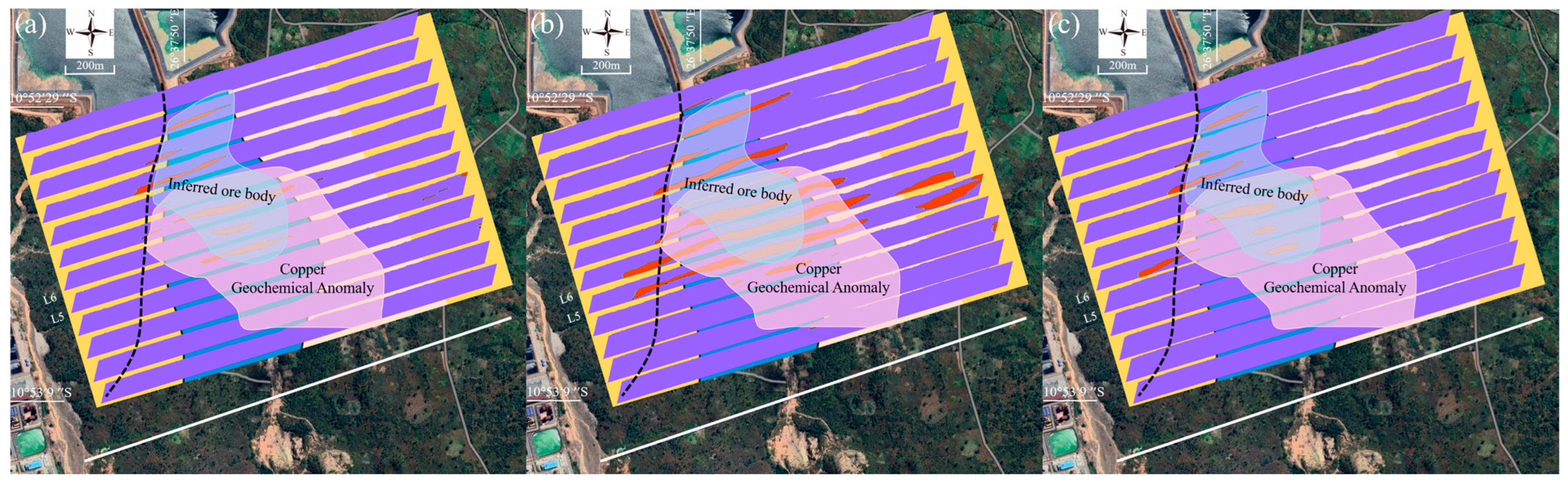
Owing to the limited number of boreholes available in the survey area, the screening thresholds were not derived from a formal population-based statistical optimization. Instead, they were empirically calibrated using the physical-property responses associated with the borehole-confirmed mineralized intervals. The lower limit of ${\log }_{10}\left(\rho \right)$ observed within the principal mineralized interval was approximately 2.5, while the minimum corresponding chargeability was approximately 0.45. These values were therefore adopted as the baseline resistivity and chargeability thresholds. The elevation threshold of 1100 m was selected because it approximately corresponds to the lowest elevation of the borehole-confirmed mineralized intervals. In addition, the sensitivity and vertical resolution of the chargeability inversion decrease with depth, making the deeper chargeability distribution less reliably constrained. Consequently, inversion results below an elevation of 1100 m were not used for target delineation. Based on these observations, the baseline screening criteria for candidate mineralized zones were defined as ${\log }_{10}\left(\rho \right)\ge 2.5$, $\eta \ge 0.45$, and elevation ≥1100 m. To evaluate the dependence of the delineated target on the selected thresholds, the classification procedure was repeated using two alternative threshold combinations. The first test was designed to represent a scenario in which mineralization may be associated with stronger polarization but relatively lower resistivity than observed in the borehole-constrained interval. In this case, the resistivity threshold was reduced to ${\log }_{10}\left(\rho \right)\ge 2.4$, while the chargeability threshold was kept at $\eta \ge 0.45$. The second test was designed to represent a scenario in which mineralization may have weaker polarization characteristics. In this case, a higher resistivity threshold of ${\log }_{10}\left(\rho \right)\ge 2.6$ was used together with a lower chargeability threshold of $\eta \ge 0.4$. These two threshold-perturbation tests were used to examine whether the delineated target was sensitive to reasonable variations in the assumed resistivity–chargeability relationship.

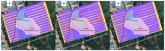
Using the joint screening criteria, the classification results from all survey lines were projected into three-dimensional space, and anomalies satisfying the resistivity–chargeability criteria and showing continuity between adjacent lines were delineated. As shown in Figure 8, the principal composite anomaly is located east of, and locally adjacent to, the inferred structural interface. It trends approximately north–south to north-northwest–south-southeast and can be traced across multiple survey lines. The anomaly exhibits banded, lenticular, and locally irregular geometries rather than a simple tabular form. To evaluate the influence of threshold selection, the delineation was repeated using two alternative resistivity–chargeability combinations. Changes in the thresholds mainly affected the peripheral extent and local continuity of the classified anomalies, whereas the principal overlapping anomaly remained largely unchanged. This result indicates that the position of the core candidate mineralized zone is relatively stable.

Figure 8. Distribution and threshold sensitivity of the inferred concealed copper–cobalt mineralized zone. (a) Baseline delineation using ${\mathrm{l}\mathrm{o}\mathrm{g}}_{10}\left(\rho \right)\ge 2.5$, $\eta \ge 0.45$ and and elevation ≥1100 m, based on the lower resistivity and chargeability limits and the lowest elevation observed within the borehole-confirmed mineralized intervals. (b) Sensitivity test with a reduced resistivity threshold of log⁡₁₀ (ρ) ≥ 2.4 and chargeability threshold of η ≥ 0.45, representing a scenario of stronger polarization but relatively lower resistivity. (c) Sensitivity test with log⁡₁₀ (ρ) ≥2.6 and η ≥ 0.4, representing a scenario of weaker polarization characteristics. The elevation threshold is fixed at 1100 m in all cases.

The delineated anomaly also shows a clear spatial relationship with the regional geological and geochemical framework. The stable core is located mainly within the Roan Group, east of the inferred electrical structural interface, and lies within or near the margin of the surface copper geochemical anomaly. This spatial correspondence suggests a possible relationship between near-surface copper enrichment and the deeper electrical-polarization response. However, the geochemical and geophysical anomaly boundaries do not coincide completely, indicating that the surface copper anomaly cannot be used directly to define the geometry of the concealed mineralized body. By integrating resistivity, chargeability, borehole constraints, the inferred structural interface, geological-unit distribution, and copper geochemical information, a candidate concealed mineralized zone was identified in the Ksignal area. Its continuity across multiple survey lines, stability under moderate threshold variations, location within the Roan Group, and spatial association with the copper geochemical anomaly support its designation as a priority target for subsequent drilling and geological verification.

These results show that, in geologically complex areas, a single geophysical parameter cannot be directly equated with an orebody. Resistivity anomalies may be caused by mineralization, but they may also reflect water-bearing fractured zones, conductive cover, clay alteration or surface water. Chargeability anomalies generally indicate strong interfacial polarization, but they can also be influenced by clay minerals, complex pore structures, magnetic minerals or mining-related accumulations. We therefore did not use any single-parameter anomaly as an orebody criterion. Instead, interpretation was constrained jointly by resistivity, chargeability, borehole information, structural interfaces and copper geochemical anomalies.

The relationship between copper geochemical anomalies and geophysical anomalies is important for interpretation. Areas where the two overlap can be regarded as favourable zones jointly indicated by near-surface elemental enrichment and deep physical-property anomalies. Local offsets may reflect weathering, leaching and secondary migration [50]. Copper geochemical anomalies are therefore useful references for evaluating the geological significance of geophysical anomalies, but should not be used directly to define the boundaries of deep orebodies. Multi-line interpretation also reduces the uncertainty associated with judging anomaly continuity from a single profile, and helps identify the trend and spatial association of anomalies along structural interfaces.

The target delineation presented in this study should be regarded as a geophysical interpretation rather than a uniquely resolved geological boundary. The inversion results remain affected by transmitter geometry, receiver elevation, topographic relief, survey-line coverage and data noise. The joint resistivity–chargeability interpretation was conservatively restricted to model cells above an elevation of 1100 m. This elevation threshold represents a conservative interpretation limit. To reduce uncertainties associated with terrain and receiver height, a high-resolution topographic surface was obtained using a mapping UAV, while the receiver elevations were determined from the onboard GPS records. These measured elevations were incorporated into the survey geometry used for data processing and inversion. The resulting resistivity and chargeability values are effective physical-property parameters at a given investigation scale and cannot be directly converted into ore grade, mineral abundance or resource estimates. We therefore describe the anomaly as an inferred concealed mineralized body or a candidate mineralized zone, rather than as a verified orebody boundary.

4. Conclusions

This study delineates a candidate concealed copper–cobalt mineralized zone in the Ksignal area of the Kambove district, Democratic Republic of the Congo, through an integrated interpretation of UAV-based SATEM data, borehole constraints and copper geochemical anomalies. The inversion results reveal clear electrical zonation across the inferred electrical structural interface. West of the interface, the subsurface is generally characterized by relatively high resistivity and low chargeability, whereas a composite resistivity–chargeability anomaly occurs to the east. The delineated anomaly is continuous across multiple survey lines, corresponds spatially with the copper geochemical anomaly, and trends from near north–south to north-northwest. These features suggest that the candidate zone is controlled by the inferred electrical structural interface and associated tectonic slices. The results show that SATEM multiparameter data interpretation can provide useful constraints for deep and peripheral exploration in mature mining districts. The delineated zone remains a geophysical target rather than a verified orebody boundary, and its mineralization significance and spatial extent require further validation by drilling and rock physical-property testing.

References

- Sovacool, B.K.; Ali, S.H.; Bazilian, M.; Radley, B.; Nemery, B.; Okatz, J.; Mulvaney, D. Sustainable Minerals and Metals for a Low-Carbon Future. Science 2020, 367, 30–33. [Google Scholar] [CrossRef] [Scilit] [PubMed]
- Boer, L.; Pescatori, A.; Stuermer, M. Energy Transition Metals: Bottleneck for Net-Zero Emissions? J. Eur. Econ. Assoc. 2024, 22, 200–229. [Google Scholar] [CrossRef] [Scilit]
- Li, W.; Erickson, E.M.; Manthiram, A. High-Nickel Layered Oxide Cathodes for Lithium-Based Automotive Batteries. Nat. Energy 2020, 5, 26–34. [Google Scholar] [CrossRef] [Scilit]
- Hitzman, M.W.; Broughton, D.; Selley, D.; Woodhead, J.; Wood, D.; Bull, S. The Central African Copperbelt: Diverse Stratigraphic, Structural, and Temporal Settings in the World’s Largest Sedimentary Copper District. In Geology and Genesis of Major Copper Deposits and Districts of the World: A Tribute to Richard H. Sillitoe; Society of Economic Geologists: Littleton, CO, USA, 2012. [Google Scholar]
- Banza Lubaba Nkulu, C.; Casas, L.; Haufroid, V.; De Putter, T.; Saenen, N.D.; Kayembe-Kitenge, T.; Musa Obadia, P.; Kyanika Wa Mukoma, D.; Lunda Ilunga, J.-M.; Nawrot, T.S. Sustainability of Artisanal Mining of Cobalt in DR Congo. Nat. Sustain. 2018, 1, 495–504. [Google Scholar] [CrossRef] [Scilit] [PubMed]
- Cailteux, J.; Kampunzu, A.; Lerouge, C.; Kaputo, A.; Milesi, J. Genesis of Sediment-Hosted Stratiform Copper–Cobalt Deposits, Central African Copperbelt. J. Afr. Earth Sci. 2005, 42, 134–158. [Google Scholar] [CrossRef] [Scilit]
- Capistrant, P.L.; Hitzman, M.W.; Wood, D.; Kelly, N.M.; Williams, G.; Zimba, M.; Kuiper, Y.; Jack, D.; Stein, H. Geology of the Enterprise Hydrothermal Nickel Deposit, North-Western Province, Zambia. Econ. Geol. 2015, 110, 9–38. [Google Scholar] [CrossRef] [Scilit]
- Dewaele, S.; Muchez, P.; Vets, J.; Fernandez-Alonzo, M.; Tack, L. Multiphase Origin of the Cu–Co Ore Deposits in the Western Part of the Lufilian Fold-and-Thrust Belt, Katanga (Democratic Republic of Congo). J. Afr. Earth Sci. 2006, 46, 455–469. [Google Scholar] [CrossRef] [Scilit]
- Herrington, R. Road Map to Mineral Supply. Nat. Geosci. 2013, 6, 892–894. [Google Scholar] [CrossRef] [Scilit]
- McCuaig, T.C.; Hronsky, J.M. The Mineral System Concept: The Key to Exploration Targeting; Society of Economic Geologists: Littleton, CO, USA, 2014. [Google Scholar]
- Jowitt, S.M.; Mudd, G.M.; Thompson, J.F. Future Availability of Non-Renewable Metal Resources and the Influence of Environmental, Social, and Governance Conflicts on Metal Production. Commun. Earth Environ. 2020, 1, 13. [Google Scholar] [CrossRef] [Scilit]
- Northey, S.; Mohr, S.; Mudd, G.M.; Weng, Z.; Giurco, D. Modelling Future Copper Ore Grade Decline Based on a Detailed Assessment of Copper Resources and Mining. Resour. Conserv. Recycl. 2014, 83, 190–201. [Google Scholar] [CrossRef] [Scilit]
- Xue, G.; Wu, X.; Chen, W.; Zhou, N. Grounded-Source Short Offset Transient Electromagnetic Method: Theory and Applications in Deep Mineral Exploration. Sci. China Earth Sci. 2025, 68, 626–638. [Google Scholar] [CrossRef] [Scilit]
- Di, Q.-Y.; Fang, G.-Y.; Zhang, Y.-M. Research of the surface electromagnetic prospecting (SEP) system. Chin. J. Geophys. 2013, 56, 3629–3639. [Google Scholar] [CrossRef]
- Smith, R. Electromagnetic Induction Methods in Mining Geophysics from 2008 to 2012. Surv. Geophys. 2014, 35, 123–156. [Google Scholar] [CrossRef] [Scilit]
- Yang, D.; Fournier, D.; Kang, S.; Oldenburg, D.W. Deep Mineral Exploration Using Multi-Scale Electromagnetic Geophysics: The Lalor Massive Sulphide Deposit Case Study. Can. J. Earth Sci. 2019, 56, 544–555. [Google Scholar] [CrossRef] [Scilit]
- Wu, X.; Rao, L.-T.; Luan, X.-D.; Shi, J.-J.; Wang, Y.-B. Design and Development of a Semiairborne Transient Electromagnetic System. Geophysics 2024, 89, E255–E266. [Google Scholar] [CrossRef] [Scilit]
- Mogi, T.; Kusunoki, K.; Kaieda, H.; Ito, H.; Jomori, A.; Jomori, N.; Yuuki, Y. Grounded Electrical-Source Airborne Transient Electromagnetic (GREATEM) Survey of Mount Bandai, North-Eastern Japan. Explor. Geophys. 2009, 40, 1–7. [Google Scholar] [CrossRef] [Scilit]
- Kotowski, P.O.; Becken, M.; Thiede, A.; Schmidt, V.; Schmalzl, J.; Ueding, S.; Klingen, S. Evaluation of a Semi-Airborne Electromagnetic Survey Based on a Multicopter Aircraft System. Geosciences 2022, 12, 26. [Google Scholar] [CrossRef] [Scilit]
- Wu, X.; Xue, G.Q.; Fang, G.Y.; Li, X.; Ji, Y. The Development and Applications of the Semi-Airborne Electromagnetic System in China. IEEE Access 2019, 7, 104956–104966. [Google Scholar] [CrossRef] [Scilit]
- Associates Australasia Pty. Ltd. TURAIR: A Recent Development in Semi-Airborne Electromagnetic Prospecting. Explor. Geophys. 1971, 2, 25–45. [Google Scholar] [CrossRef] [Scilit]
- Elliott, P. The Principles and Practice of FLAIRTEM. Explor. Geophys. 1998, 29, 58–59. [Google Scholar] [CrossRef] [Scilit]
- Becken, M.; Nittinger, C.G.; Smirnova, M.; Steuer, A.; Martin, T.; Petersen, H.; Meyer, U.; Mörbe, W.; Yogeshwar, P.; Tezkan, B. DESMEX: A Novel System Development for Semi-Airborne Electromagnetic Exploration. Geophysics 2020, 85, E253–E267. [Google Scholar] [CrossRef] [Scilit]
- Liu, Y.; Yin, C.; Qiu, C.; Hui, Z.; Zhang, B.; Ren, X.; Weng, A. 3-D Inversion of Transient EM Data with Topography Using Unstructured Tetrahedral Grids. Geophys. J. Int. 2019, 217, 301–318. [Google Scholar] [CrossRef] [Scilit]
- Lu, J.; Wang, X.; Xu, Z.; Zhdanov, M.S.; Guo, M.; Teng, M.; Liu, Z. Quasi-2-D Robust Inversion of Semi-Airborne Transient Electromagnetic Data with IP Effects. IEEE Trans. Geosci. Remote Sens. 2022, 60, 2008210. [Google Scholar] [CrossRef] [Scilit]
- Wu, X.; Xue, G.-Q.; Liu, Y.; Wang, Y.-B.; Zhang, J.-E.; Chen, W.-Y.; He, L.-F.; Zhao, Y.-G. Brownfields Exploration Using Semi-Airborne Transient Electromagnetic Surveys at the Giant Bayan Obo REE-Nb-Fe Deposit, Inner Mongolia, China. Ore Geol. Rev. 2025, 181, 106610. [Google Scholar] [CrossRef] [Scilit]
- Steuer, A.; Smirnova, M.; Becken, M.; Schiffler, M.; Günther, T.; Rochlitz, R.; Yogeshwar, P.; Mörbe, W.; Siemon, B.; Costabel, S. Comparison of Novel Semi-Airborne Electromagnetic Data with Multi-Scale Geophysical, Petrophysical and Geological Data from Schleiz, Germany. J. Appl. Geophys. 2020, 182, 104172. [Google Scholar] [CrossRef] [Scilit]
- He, K.; Wang, X.; Guo, M.; Wang, S.; Yi, G.; Xie, X.; Guo, Y. Spatially Constrained Inversion of Semi-Airborne Transient Electromagnetic Data Based on a Mixed Norm. J. Appl. Geophys. 2022, 200, 104616. [Google Scholar] [CrossRef] [Scilit]
- Pelton, W.H.; Ward, S.; Hallof, P.; Sill, W.; Nelson, P.H. Mineral Discrimination and Removal of Inductive Coupling with Multifrequency IP. Geophysics 1978, 43, 588–609. [Google Scholar] [CrossRef] [Scilit]
- Wong, J. An Electrochemical Model of the Induced-Polarization Phenomenon in Disseminated Sulfide Ores. Geophysics 1979, 44, 1245–1265. [Google Scholar] [CrossRef] [Scilit]
- Marchant, D.; Haber, E.; Oldenburg, D.W. Three-Dimensional Modeling of IP Effects in Time-Domain Electromagnetic Data. Geophysics 2014, 79, E303–E314. [Google Scholar] [CrossRef] [Scilit]
- Macnae, J. Quantifying Airborne Induced Polarization Effects in Helicopter Time Domain Electromagnetics. J. Appl. Geophys. 2016, 135, 495–502. [Google Scholar] [CrossRef] [Scilit]
- Revil, A.; Vaudelet, P.; Su, Z.; Chen, R. Induced Polarization as a Tool to Assess Mineral Deposits: A Review. Minerals 2022, 12, 571. [Google Scholar] [CrossRef] [Scilit]
- Cailteux, J.L.; De Putter, T. The Neoproterozoic Katanga Supergroup (DR Congo): State-of-the-Art and Revisions of the Lithostratigraphy, Sedimentary Basin and Geodynamic Evolution. J. Afr. Earth Sci. 2019, 150, 522–531. [Google Scholar] [CrossRef] [Scilit]
- Kampunzu, A.; Cailteux, J.; Kamona, A.; Intiomale, M.; Melcher, F. Sediment-Hosted Zn–Pb–Cu Deposits in the Central African Copperbelt. Ore Geol. Rev. 2009, 35, 263–297. [Google Scholar] [CrossRef] [Scilit]
- Zientek, M.L.; Bliss, J.D.; Broughton, D.W.; Christie, M.; Denning, P.; Hayes, T.S.; Hitzman, M.W.; Horton, J.D.; Frost-Killian, S.; Jack, D.J. Sediment-Hosted Stratabound Copper Assessment of the Neoproterozoic Roan Group, Central African Copperbelt, Katanga Basin, Democratic Republic of the Congo and Zambia; US Geological Survey: Reston, VA, USA, 2014.
- Hitzman, M.; Kirkham, R.; Broughton, D.; Thorson, J.; Selley, D. The Sediment-Hosted Stratiform Copper Ore System; Society of Economic Geologists: Littleton, CO, USA, 2005. [Google Scholar] [CrossRef] [Scilit]
- Wu, X.; Xue, G.; Gao, Y.; Wang, Y.; Li, Y.; Qian, Z.; Zhao, Y.; Xue, J.; Cui, S.; Zhou, N. A Method of Deep Mineralization Potential Exploration Based on UAVs and Its Application in an Abandoned Mine in the Democratic Republic of the Congo. Drones 2026, 10, 293. [Google Scholar] [CrossRef] [Scilit]
- Van Langendonck, S.; Muchez, P.; Dewaele, S.; Kalubi, A.K.; Cailteux, J. Petrographic and Mineralogical Study of the Sediment-Hosted Cu-Co Ore Deposit at Kambove West in the Central Part of the Katanga Copperbelt (DRC). Geol. Belg. 2013, 16, 179–190. [Google Scholar]
- Saintilan, N.J.; Selby, D.; Creaser, R.A.; Dewaele, S. Sulphide Re-Os Geochronology Links Orogenesis, Salt and Cu-Co Ores in the Central African Copperbelt. Sci. Rep. 2018, 8, 14946. [Google Scholar] [CrossRef] [Scilit] [PubMed]
- El Desouky, H.A.; Muchez, P.; Cailteux, J. Two Cu–Co Sulfide Phases and Contrasting Fluid Systems in the Katanga Copperbelt, Democratic Republic of Congo. Ore Geol. Rev. 2009, 36, 315–332. [Google Scholar] [CrossRef] [Scilit]
- Mambwe, P.; Kipata, L.; Chabu, M.; Muchez, P.; Lubala, T.; Jébrak, M.; Delvaux, D. Sedimentology of the Shangoluwe Breccias and Timing of the Cu Mineralisation (Katanga Supergroup, DR of Congo). J. Afr. Earth Sci. 2017, 132, 1–15. [Google Scholar] [CrossRef] [Scilit]
- Van Wilderode, J.; Debruyne, D.; Torremans, K.; Elburg, M.A.; Vanhaecke, F.; Muchez, P. Metal Sources for the Nkana and Konkola Stratiform Cu–Co Deposits (Zambian Copperbelt): Insights from Sr and Nd Isotope Ratios. Ore Geol. Rev. 2015, 67, 127–138. [Google Scholar] [CrossRef] [Scilit]
- Cailteux, J. Lithostratigraphy of the Neoproterozoic Shaba-Type (Zaire) Roan Supergroup and Metallogenesis of Associated Stratiform Mineralization. J. Afr. Earth Sci. 1994, 19, 279–301. [Google Scholar] [CrossRef] [Scilit]
- Wu, X.; Xue, G.; Zhao, Y.; Lv, P.; Zhou, Z.; Shi, J. A Deep Learning Estimation of the Earth Resistivity Model for the Airborne Transient Electromagnetic Observation. J. Geophys. Res. Solid Earth 2022, 127, e2021JB023185. [Google Scholar] [CrossRef] [Scilit]
- Wu, X.; Xue, G.Q.; He, Y.M.; Xue, J.J. Removal of Multisource Noise in Airborne Electromagnetic Data Based on Deep Learning. Geophysics 2020, 85, B207–B222. [Google Scholar] [CrossRef] [Scilit]
- Oldenburg, D.W. Computation of ColeCole Parameters from IP Data. Geophysics 1997, 62, 436–448. [Google Scholar] [CrossRef] [Scilit]
- Stolz, E.M.; Macnae, J. Evaluating EM Waveforms by Singular-Value Decomposition of Exponential Basis Functions. Geophysics 1998, 63, 64–74. [Google Scholar] [CrossRef] [Scilit]
- Kratzer, T.; Macnae, J.C. Induced Polarization in Airborne EM. Geophysics 2012, 77, E317–E327. [Google Scholar] [CrossRef] [Scilit]
- Gigler, G.M.; Kinnaird, J.A. Element Mobility in the Weathering Environment and Surface Vectors to Mineralisation—A Case Study from the Mashitu South Cu-Co Deposit, Katanga, Democratic Republic of Congo. J. Geochem. Explor. 2017, 183, 127–137. [Google Scholar] [CrossRef] [Scilit]
Disclaimer/Publisher’s Note: The statements, opinions and data contained in all publications are solely those of the individual author(s) and contributor(s) and not of MDPI and/or the editor(s). MDPI and/or the editor(s) disclaim responsibility for any injury to people or property resulting from any ideas, methods, instructions or products referred to in the content. |
© 2026 by the authors. Licensee MDPI, Basel, Switzerland. This article is an open access article distributed under the terms and conditions of the Creative Commons Attribution (CC BY) license.