A Stochastic Gauss–Newton Framework with Full-Data Line Search for Efficient 3D Magnetotelluric Inversion

Abstract

3D magnetotelluric (MT) inversion based on the Gauss–Newton (GN) framework plays an important role in deep mineral exploration by imaging subsurface electrical conductivity structures. However, large-scale 3D MT inversion remains computationally expensive due to the high cost of sensitivity-matrix construction. To address this challenge, we develop a stochastic Gauss–Newton (SGN) framework that reduces computational cost through random data subsampling while preserving the practical convergence behavior of GN inversion. In the proposed framework, only a randomly selected subset of data is used to approximate the GN search direction. By exploiting a key property of MT forward modelling, namely that responses at all receivers are obtained simultaneously for each frequency, the line search is performed using the full dataset, ensuring stable convergence of the inversion process. The SGN framework is validated using both a synthetic multiblock model and a field dataset from the Akebasitao area in Xinjiang, China. The recovered models remain highly consistent with those obtained using conventional full-data Gauss–Newton inversion across a wide range of sampling ratios. For the synthetic example, reducing the sampling ratio from 100% to 10% decreases peak memory consumption from approximately 433 GB to 242 GB and reduces runtime from 86.8 h to 23.9 h while maintaining comparable inversion quality. Similar computational savings are achieved for the field-data inversion. The field application successfully recovers the major conductive structures along the margins of the intrusion that are associated with hydrothermal alteration and fluid activity, highlighting the capability of SGN to delineate geologically meaningful targets relevant to deep mineral exploration. These results demonstrate that SGN provides an efficient and scalable approach for large-scale 3D MT inversion.

1. Introduction

3D magnetotelluric (MT) inversion has become a standard tool for imaging subsurface electrical conductivity structures [1,2,3,4,5,6]. Its applications range from mineral exploration [7,8,9] and geothermal resource assessment [10,11] to crustal tectonic studies [12,13,14,15,16,17,18,19,20,21,22]. Despite its wide applicability, 3D MT inversion remains computationally demanding, particularly for large-scale problems with fine discretization.

Among the available inversion strategies, the Gauss–Newton (GN) method [23,24,25,26] and its variants, such as the Occam approach [27,28,29], are widely used due to their fast convergence and their ability to incorporate second-order information. These methods have been successfully applied in both model-space and data-space inversion frameworks. In the GN framework, the inversion relies on the sensitivity (Jacobian) matrix, which maps perturbations in model parameters to variations in observed data [30]. The Jacobian is typically of size $N_d\times N_m$, where $N_d$ denotes the number of observations and $N_m$ the number of model parameters. For large-scale 3D MT problems, both $N_d$ and $N_m$ can be very large, making the computation of the Jacobian and the solution of the associated normal equations the dominant computational bottleneck.

To alleviate this challenge, a variety of acceleration strategies have been proposed, including reduced-basis approximations [31], quasi-Newton methods such as L-BFGS [32,33,34], and stochastic approaches [35] that aim to reduce the computational cost per iteration. Stochastic optimisation methods have been extensively developed in machine learning, where stochastic gradient descent (SGD) and its variants approximate the full gradient using randomly selected subsets of data (mini-batches) [36,37,38,39,40]. This strategy significantly reduces computational cost and has proven effective for large-scale optimisation problems. However, SGD-type methods typically require a large number of iterations to converge. This slow convergence arises not only from the use of noisy gradient estimates but also from the lack of accurate objective function evaluation when only a subset of data is used. These limitations motivate the integration of stochastic sampling with second-order methods, which provide more reliable search directions and improved convergence behaviour.

Stochastic second-order optimization methods have been extensively studied for large-scale inverse and optimization problems. Representative approaches include subsampled Newton methods [41,42], the Newton–Sketch framework [43], and stochastic Gauss–Newton (SGN) variants [44,45]. Theoretical foundations of these methods have been well established in the above optimization literature, where their convergence properties are analyzed under standard assumptions. These methods reduce computational cost by constructing approximate gradients, Jacobians, or Hessians from randomly selected subsets of data while retaining the essential characteristics of second-order optimization. In geophysical inversion, stochastic strategies have been investigated in a variety of applications, including seismic inversion [46,47] and airborne electromagnetic inversion [48,49,50,51,52]. These studies demonstrated that substantial computational savings can be achieved by evaluating the search direction using only a subset of observations at each iteration.

Motivated by these observations, we develop the SGN framework for 3D MT inversion. In the proposed framework, only a randomly selected subset of observations is used to construct the Jacobian matrix and residual vector, yielding an approximate search direction through a reduced system of normal equations. A key feature of MT forward modelling is that, for a given frequency, a single forward simulation simultaneously provides responses at all receiver locations. Therefore, even though only a subset of observations is used to construct the Jacobian matrix, the objective function can still be evaluated exactly using the complete dataset. This property enables the step length to be determined through a line search based on the full-data objective function, thereby ensuring monotonic reduction of the true objective function despite the stochastic approximation used in the search direction.

Unlike data-space Gauss–Newton approaches [28], which reduce the cost of solving the normal equations while still requiring construction of the full Jacobian matrix, the proposed method directly reduces the cost of Jacobian construction through stochastic subsampling. Furthermore, many existing stochastic geophysical inversion approaches require additional procedures to estimate the contribution of unsampled observations [50]. Missing responses are often reconstructed or approximated using compressed sensing or related data-recovery techniques [53], introducing additional computational overhead and potential approximation errors. By exploiting the characteristics of MT forward modelling, the proposed framework avoids such reconstruction procedures, making SGN particularly attractive for large-scale 3D MT inversion.

The remainder of this paper is organized as follows. Section 2 introduces the proposed SGN framework and its implementation for 3D MT inversion. Section 3 presents synthetic and field examples together with computational performance analyses. Section 4 discusses the results, and Section 5 summarizes the main conclusions.

2. Methodology

2.1. Standard Gauss–Newton Inversion with Full Data

The MT inverse problem seeks to recover a subsurface resistivity model from observed data. The inverse problem is formulated as a regularized least-squares objective function

$$\mathsf{\Phi }\left(\mathbf{m}\right)={\displaystyle \frac{1}{2}}{∥{\mathbf{W}}_d\left[\mathbf{F}\left(\mathbf{m}\right)-{\mathbf{d}}_{\mathrm{obs}}\right]∥}_2^2+{\displaystyle \frac{1}{2}}\beta {∥{\mathbf{W}}_m(\mathbf{m}-{\mathbf{m}}_0)∥}_2^2,$$

(1)

where the vector ${\mathbf{d}}_{\mathrm{obs}}\in {\mathbb{R}}^{N_d}$ denotes the observed data, and the vectors $\mathbf{m},{\mathbf{m}}_0\in {\mathbb{R}}^{N_m}$ represent the model and reference model in logarithmic resistivity space, respectively. The forward operator $\mathbf{F}\left(\mathbf{m}\right)$ computes the predicted responses. ${\mathbf{W}}_m$ is the model regularization matrix, and $\beta$ is the regularization parameter. The data weighting matrix ${\mathbf{W}}_d$ is defined as a diagonal matrix:

$${\mathbf{W}}_d=\mathrm{diag}\left({\displaystyle \frac{1}{{\sigma }_1}},{\displaystyle \frac{1}{{\sigma }_2}},\dots ,{\displaystyle \frac{1}{{\sigma }_{N_d}}}\right),$$

(2)

where ${\sigma }_i$ denotes the estimated standard deviation of each data component obtained from impedance tensor error analysis, ensuring that each observation is properly normalized according to its noise level.

Differentiating the objective function with respect to $\mathbf{m}$ yields the gradient

$$\mathbf{g}\left(\mathbf{m}\right)=\mathbf{J}{\left(\mathbf{m}\right)}^T{\mathbf{W}}_d^T{\mathbf{W}}_d\mathbf{r}+\beta {\mathbf{W}}_m^T{\mathbf{W}}_m(\mathbf{m}-{\mathbf{m}}_0),$$

(3)

where $\mathbf{J}\left(\mathbf{m}\right)=\partial \mathbf{F}\left(\mathbf{m}\right)/\partial \mathbf{m}\in {\mathbb{R}}^{N_d\times N_m}$ is the Jacobian (sensitivity) matrix, and $\mathbf{r}=\mathbf{F}\left(\mathbf{m}\right)-{\mathbf{d}}_{\mathrm{obs}}$ is the residual vector.

The inversion problem is nonlinear and can be solved iteratively using the GN method. At iteration k, the model update (or search direction) $\Delta {\mathbf{m}}_k$ is obtained by solving the normal equations

$$\left[{\mathbf{J}}_k^T{\mathbf{W}}_d^T{\mathbf{W}}_d{\mathbf{J}}_k+\beta {\mathbf{W}}_m^T{\mathbf{W}}_m+\lambda \mathbf{I}\right]\Delta {\mathbf{m}}_k=-{\mathbf{g}}_k,$$

(4)

where ${\mathbf{J}}_k=\mathbf{J}\left({\mathbf{m}}_k\right)$, ${\mathbf{g}}_k=\mathbf{g}\left({\mathbf{m}}_k\right)$, and $\lambda$ is a small damping parameter (Levenberg–Marquardt type) [54,55] introduced for numerical stability. In this work, we use a fixed small $\lambda$ (e.g., ${10}^{-6}$).

Once $\Delta {\mathbf{m}}_k$ is computed, a line search finds the step length ${\alpha }_k>0$ that satisfies the Armijo condition or simply minimizes $\mathsf{\Phi }({\mathbf{m}}_k+\alpha \Delta {\mathbf{m}}_k)$ [56]. The model is then updated according to

$${\mathbf{m}}_{k+1}={\mathbf{m}}_k+{\alpha }_k\Delta {\mathbf{m}}_k.$$

(5)

The computational bottleneck lies in constructing the Jacobian matrix ${\mathbf{J}}_k$, which requires solving one adjoint linear system per data component, resulting in a total of $N_d$ adjoint solves [30,57].

2.2. Stochastic Sensitivity Approximation via Data Subsampling

To reduce the cost of each GN iteration, we compute the sensitivity matrix using only a randomly selected subset of the data. At iteration k, a subset $S_k\subset \{1,\dots ,N_d\}$ is generated by uniform random sampling from the complete data vector, with size $|S_k|=p{N}_d$, where $p\in (0,1]$ denotes the sampling ratio. Thus, each observation has an equal probability of being selected, independent of frequency, station location, and impedance tensor component.

Let ${\tilde{\mathbf{J}}}_k\in {\mathbb{R}}^{p{N}_d\times N_m}$ and ${\tilde{\mathbf{r}}}_k\in {\mathbb{R}}^{p{N}_d}$ denote the Jacobian and residual restricted to the selected indices, and let ${\tilde{\mathbf{W}}}_d$ be the corresponding data weighting matrix. The SGN step is then obtained by solving the normal equations formed using the reduced sensitivity matrix

$$\left[{\tilde{\mathbf{J}}}_k^T{\tilde{\mathbf{W}}}_d^T{\tilde{\mathbf{W}}}_d{\tilde{\mathbf{J}}}_k+\beta {\mathbf{W}}_m^T{\mathbf{W}}_m+\lambda \mathbf{I}\right]\Delta {\tilde{\mathbf{m}}}_k=-{\tilde{\mathbf{g}}}_k,$$

(6)

where

$${\tilde{\mathbf{g}}}_k={\tilde{\mathbf{J}}}_k^T{\tilde{\mathbf{W}}}_d^T{\tilde{\mathbf{W}}}_d{\tilde{\mathbf{r}}}_k+\beta {\mathbf{W}}_m^T{\mathbf{W}}_m({\mathbf{m}}_k-{\mathbf{m}}_0)$$

(7)

is the stochastic approximation of the full gradient.

The resulting $\Delta {\tilde{\mathbf{m}}}_k$ serves as an approximate search direction for the GN iteration. Since only a fraction p of the data is used, the cost of constructing ${\tilde{\mathbf{J}}}_k$ is reduced from $O\left(N_d\right)$ adjoint solves to $O\left(p{N}_d\right)$, leading to a substantial reduction in computational cost, while the cost associated with solving the normal equations is typically much smaller in comparison.

2.3. Line Search with Full-Data Objective Function

A key component of the SGN framework is that the line search is performed using the full-data objective function rather than the sampled subset. Using only the subset would lead to an inconsistent descent condition and may cause convergence instability.

Given the stochastic search direction ${\mathbf{p}}_k=\Delta {\tilde{\mathbf{m}}}_k$, the step length ${\alpha }_k$ is determined by

$${\alpha }_k=arg\underset{\alpha >0}{min}\mathsf{\Phi }({\mathbf{m}}_k+\alpha {\mathbf{p}}_k),$$

(8)

where $\mathsf{\Phi }$ is evaluated using all observed data.

This requires evaluating the forward response $\mathbf{F}({\mathbf{m}}_k+\alpha {\mathbf{p}}_k)$ for several trial step lengths. Importantly, in MT forward modeling, the dominant computational cost arises from solving the underlying field equations for each frequency. Once the field solution is obtained, responses at all receiver locations are computed through interpolation, which incurs negligible additional cost. Therefore, evaluating the full-data objective function incurs nearly the same computational cost as evaluating it on a subset, which makes SGN particularly efficient for MT inversion.

The complete SGN algorithm is summarized in Algorithm 1. In practice, a backtracking line search is performed using the full-data objective function. Starting from an initial step length $\alpha =1$, the step size is iteratively reduced by a factor of 0.5 until either the maximum number of line-search iterations is reached or the Armijo sufficient decrease condition is satisfied,

$$\mathsf{\Phi }({\mathbf{m}}_k+\alpha {\mathbf{p}}_k)\le \mathsf{\Phi }\left({\mathbf{m}}_k\right)+c\alpha \nabla \mathsf{\Phi }{\left({\mathbf{m}}_k\right)}^T{\mathbf{p}}_k,$$

(9)

where $c={10}^{-4}$ controls the sufficient decrease condition.

If no acceptable step length can be found, we reduce the regularization parameter according to a cooling strategy

$$\beta =\tau \beta ,$$

(10)

where $\tau <1$ is a prescribed cooling factor.

To monitor convergence, we use the normalized root-mean-square (NRMS) misfit

$$\mathrm{NRMS}=\sqrt{{\displaystyle \frac{1}{N_d}}{∥{\mathbf{W}}_d\left[\mathbf{F}\left(\mathbf{m}\right)-{\mathbf{d}}_{\mathrm{obs}}\right]∥}_2^2}.$$

(11)

The inversion is terminated when the NRMS falls below a prescribed tolerance or when the regularization parameter reaches a specified minimum value.

Algorithm 1 SGN for 3D MT inversion

1: Input: observed data ${\mathbf{d}}_{\mathrm{obs}}$, initial model ${\mathbf{m}}_0$, data weighting ${\mathbf{W}}_d$, model weighting ${\mathbf{W}}_m$, initial regularization parameter $\beta$, cooling factor $\tau$, minimum regularization parameter ${\beta }_{min}$, damping parameter $\lambda$, sampling ratio p, maximum iterations K, maximum line-search iterations $k_l$, NRMS tolerance $ϵ$  2: Output: inverted model ${\mathbf{m}}_k$  3: for$k=0$ to $K-1$ do  4:     Randomly select data subset $S_k\subset \{1,\dots ,N_d\}$ with $|S_k|=p{N}_d$ using uniform random sampling  5:     Extract ${\tilde{\mathbf{d}}}_{\mathrm{obs}}$, ${\tilde{\mathbf{W}}}_d$ corresponding to $S_k$  6:     Compute forward response $\mathbf{F}\left({\mathbf{m}}_k\right)$ and residual ${\mathbf{r}}_k=\mathbf{F}\left({\mathbf{m}}_k\right)-{\mathbf{d}}_{\mathrm{obs}}$  7:     Form subset residual ${\tilde{\mathbf{r}}}_k$  8:     Compute reduced Jacobian ${\tilde{\mathbf{J}}}_k$  9:     Compute stochastic gradient: $${\tilde{\mathbf{g}}}_k={\tilde{\mathbf{J}}}_k^T{\tilde{\mathbf{W}}}_d^T{\tilde{\mathbf{W}}}_d{\tilde{\mathbf{r}}}_k+\beta {\mathbf{W}}_m^T{\mathbf{W}}_m({\mathbf{m}}_k-{\mathbf{m}}_0)$$ 10:     Solve the normal equations: $$\left[{\tilde{\mathbf{J}}}_k^T{\tilde{\mathbf{W}}}_d^T{\tilde{\mathbf{W}}}_d{\tilde{\mathbf{J}}}_k+\beta {\mathbf{W}}_m^T{\mathbf{W}}_m+\lambda \mathbf{I}\right]\Delta {\tilde{\mathbf{m}}}_k=-{\tilde{\mathbf{g}}}_k$$ 11:     Perform line search to find ${\alpha }_k$ using full-data objective function $\mathsf{\Phi }\left(\mathbf{m}\right)$ 12:     if Armijo condition satisfied within $k_l$ line-search iterations then 13:         Update model: $${\mathbf{m}}_{k+1}={\mathbf{m}}_k+{\alpha }_k\Delta {\tilde{\mathbf{m}}}_k$$ 14:     else 15:         Update regularization parameter: $$\beta =\tau \beta$$ 16:     end if 17:     Compute NRMS 18:     if NRMS <= $ϵ$ or $\beta <{\beta }_{min}$ then 19:         break 20:     end if 21: end for

3. Numerical Experiments

All numerical experiments were performed on the Taiyi high-performance computing cluster at the Southern University of Science and Technology. The cluster consists of 815 compute nodes, each equipped with two Intel Xeon Gold 6148 CPUs (2.4 GHz, 20 cores per CPU; Intel, Santa Clara, CA, USA) and 192 GB of memory. All reported computational times and memory usage were measured under this computing environment.

To quantitatively assess the similarity between the models recovered using different sampling ratios and the full-data GN inversion, we compute the model root-mean-square (mRMS) difference and Pearson correlation coefficient (PCC) in the logarithmic resistivity domain within the core model region, excluding the air layers and padding cells,

$$\mathrm{mRMS}=\sqrt{{\displaystyle \frac{1}{N_m^c}}\sum _{i=1}^{N_m^c}{\left[{log}_{10}{\rho }_i^{\left(p\right)}-{log}_{10}{\rho }_i^{\left(100\right)}\right]}^2},$$

(12)

$$\mathrm{PCC}={\displaystyle \frac{{\sum }_{i=1}^{N_m^c}\left({log}_{10}{\rho }_i^{\left(p\right)}-\overline{{log}_{10}{\rho }^{\left(p\right)}}\right)\left({log}_{10}{\rho }_i^{\left(100\right)}-\overline{{log}_{10}{\rho }^{\left(100\right)}}\right)}{\sqrt{{\sum }_{i=1}^{N_m^c}{\left({log}_{10}{\rho }_i^{\left(p\right)}-\overline{{log}_{10}{\rho }^{\left(p\right)}}\right)}^2}\sqrt{{\sum }_{i=1}^{N_m^c}{\left({log}_{10}{\rho }_i^{\left(100\right)}-\overline{{log}_{10}{\rho }^{\left(100\right)}}\right)}^2}}},$$

(13)

where $N_m^c$ is the number of model parameters within the core model region, ${\rho }_i^{\left(p\right)}$ denotes the resistivity of the ith model cell obtained with sampling ratio p, and ${\rho }_i^{\left(100\right)}$ denotes the corresponding resistivity obtained from the full-data GN inversion ($p=100\%$). The overbar denotes the arithmetic mean over all model cells. Smaller mRMS values indicate higher similarity between the two recovered models, whereas PCC values closer to unity indicate stronger model agreement.

3.1. Synthetic Case

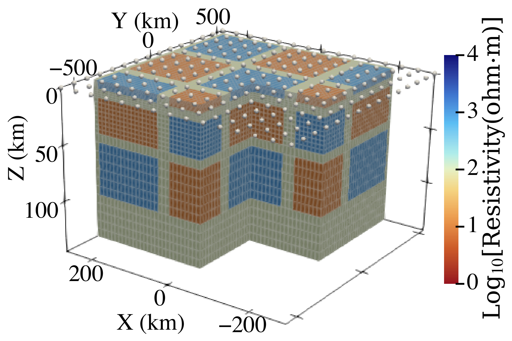
We employed a synthetic 3D MT model to validate the proposed SGN method. The model follows the well-known multi-block benchmark of [30], consisting of a 3D checkerboard distribution of 10 and 1000 ohm·m blocks embedded in a homogeneous half-space of 100 ohm·m (Figure 1). The inversion mesh is discretized with a nominal core resolution of 10 km × 20 km in the horizontal directions, padded by five cells on each lateral boundary, and 66 layers in the vertical direction. This results in a grid of 66 × 66 × 73 cells, including seven air layers. A total of 225 MT sites are arranged on a 15 × 15 regular grid covering an area of 40 km × 80 km. Forward simulations are performed at 12 logarithmically spaced periods ranging from 10 to 10,000 s.

The synthetic MT dataset used for inversion is taken from [58]. No additional random noise is added to the synthetic responses. Error floors are assigned as 5% of $|Z_{xy}|$ for $Z_{xx}$ and $Z_{xy}$, and 5% of $|Z_{yx}|$ for $Z_{yy}$ and $Z_{yx}$. A homogeneous half-space of 100 ohm·m is adopted as both the initial and reference model. The regularization parameter $\beta$ is initialized at ${10}^3$ and reduced by a factor of 0.1 to a minimum value of ${10}^{-3}$. The inversion is terminated when the NRMS reaches 1.05 or lower. We investigate 10 sampling ratios, ranging from 10% to 100%. At each SGN iteration, the data subset is randomly selected, with the stochastic sampling performed without fixing the random seed. The line search is performed using a backtracking strategy with an initial step length of 1.0, a reduction factor of 0.5, and up to 5 full-data forward evaluations per iteration. Sensitivity computation for each sampled subset is carried out using automatic differentiation [57]. All inversions are performed on 6 compute nodes (240 CPU cores) using a hybrid MPI+OpenMP parallelization scheme, with 12 MPI ranks and 20 threads per rank.

The inversion results are shown in Figure 2, and the corresponding performance metrics are summarized in

Table 1. Effect of sampling ratio on inversion accuracy, convergence behavior, and computational efficiency (Multiblock).

Sampling Ratio (%)	NRMS	Iterations	Time (h)	Peak Memory (GB)	mRMS	PCC
10	1.03	25	23.94	242.25	0.016	0.964
20	1.05	27	28.28	257.41	0.016	0.963
30	0.94	20	23.73	263.20	0.003	0.993
40	1.02	40	47.72	275.61	0.017	0.964
50	1.03	30	40.62	303.35	0.015	0.966
60	1.01	34	50.68	342.08	0.017	0.964
70	0.99	29	48.12	366.61	0.001	0.998
80	1.04	34	60.97	388.92	0.016	0.966
90	1.01	32	61.81	407.94	0.0003	0.999
100	1.04	42	86.83	433.26	-	-

. The recovered resistivity models remain highly consistent across different sampling ratios, indicating that the inversion is robust to data reduction. No noticeable structural distortion is observed even at low sampling levels. This observation is further supported by the small mRMS values (generally below 0.02) and high PCC values (0.963–0.999). The reported memory consumption corresponds to the peak memory usage recorded during the entire inversion process by the Taiyi high-performance computing cluster. Therefore, it reflects the overall memory requirement of the inversion workflow rather than the storage cost of any individual component. As the sampling ratio decreases, the peak memory requirement is substantially reduced, from approximately 433 GB at full sampling to about 242 GB at 10% sampling. A similar trend is observed for computational time, which decreases from about 86.8 hours at full sampling to 23.9 hours at 10% sampling. The reduction in both runtime and peak memory consumption demonstrates that stochastic subsampling can significantly improve computational efficiency while maintaining nearly identical inversion quality for this case.

3.2. Real-World Case

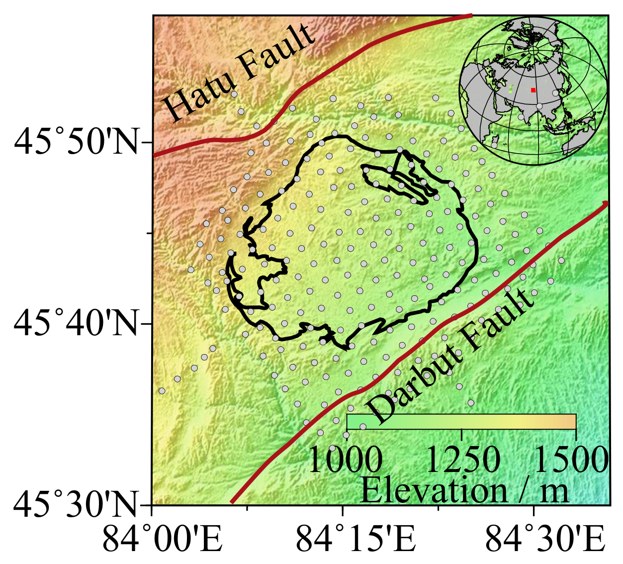
The real-world MT dataset [59] was acquired in the Houshan area of West Junggar, Xinjiang, China (Figure 3). The survey was carried out in 2013 by the electromagnetic group from China University of Geosciences (Wuhan) using Phoenix MTU-5A instruments. The acquisition consists of 16 survey lines with a spacing of approximately 2 km, forming a 3D observation network. At each site, time series data were recorded for more than 90 min and subsequently processed using standard robust techniques to obtain reliable impedance tensor estimates. The study area covers the Akebasitao pluton, a Late Carboniferous to Early Permian A-type granite intrusion.

For inversion, the model domain is discretized using a horizontal core grid of 800 m × 800 m, extended by 7 padding cells on each lateral boundary. The vertical discretization consists of 30 layers, starting from a thickness of 5 m and increasing logarithmically, together with 7 air layers, resulting in a mesh of $70\times 75\times 37$ cells. The inversion incorporates full impedance tensor data from 230 MT sites over 29 frequencies ranging from 759 Hz to 1.4 Hz. Error floors are set to 5% of $|Z_{xy}|$ for $Z_{xx}$ and $Z_{xy}$, and 5% of $|Z_{yx}|$ for $Z_{yy}$ and $Z_{yx}$. A homogeneous half-space of 600 ohm·m is adopted as both the initial and reference model. The inversion setup follows that of the synthetic case, including the regularization schedule, sampling ratios, line-search parameters, and sensitivity computation strategy. Convergence is declared when the NRMS reaches 2.00 or lower. All inversions are performed on 6 compute nodes (232 CPU cores) using a hybrid MPI+OpenMP parallelization scheme, with 29 MPI ranks and 8 threads per rank.

Figure 2. Inverted models for the multiblock case with different sampling ratios (a–j). The spheres represent the locations of MT sites.

Figure 2. Inverted models for the multiblock case with different sampling ratios (a–j). The spheres represent the locations of MT sites.

Figure 3. Map of the Akebasitao area modified from [59]. The black lines represent the surficial boundaries of the Akebasitao pluton, the red lines represent faults, and the gray circles represent the MT sites.

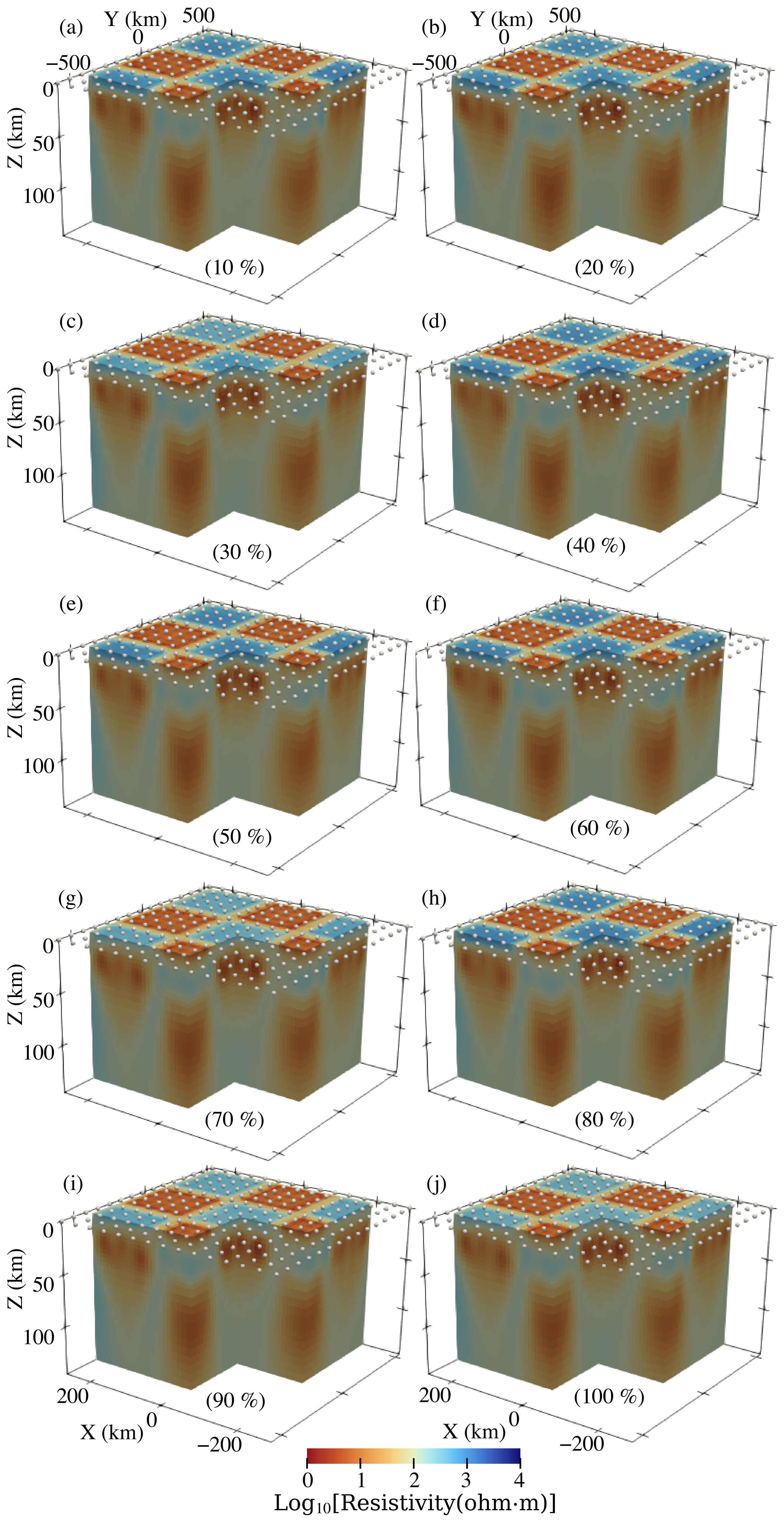
Figure 3. Map of the Akebasitao area modified from [59]. The black lines represent the surficial boundaries of the Akebasitao pluton, the red lines represent faults, and the gray circles represent the MT sites.

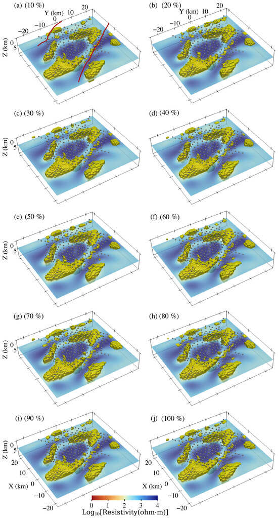
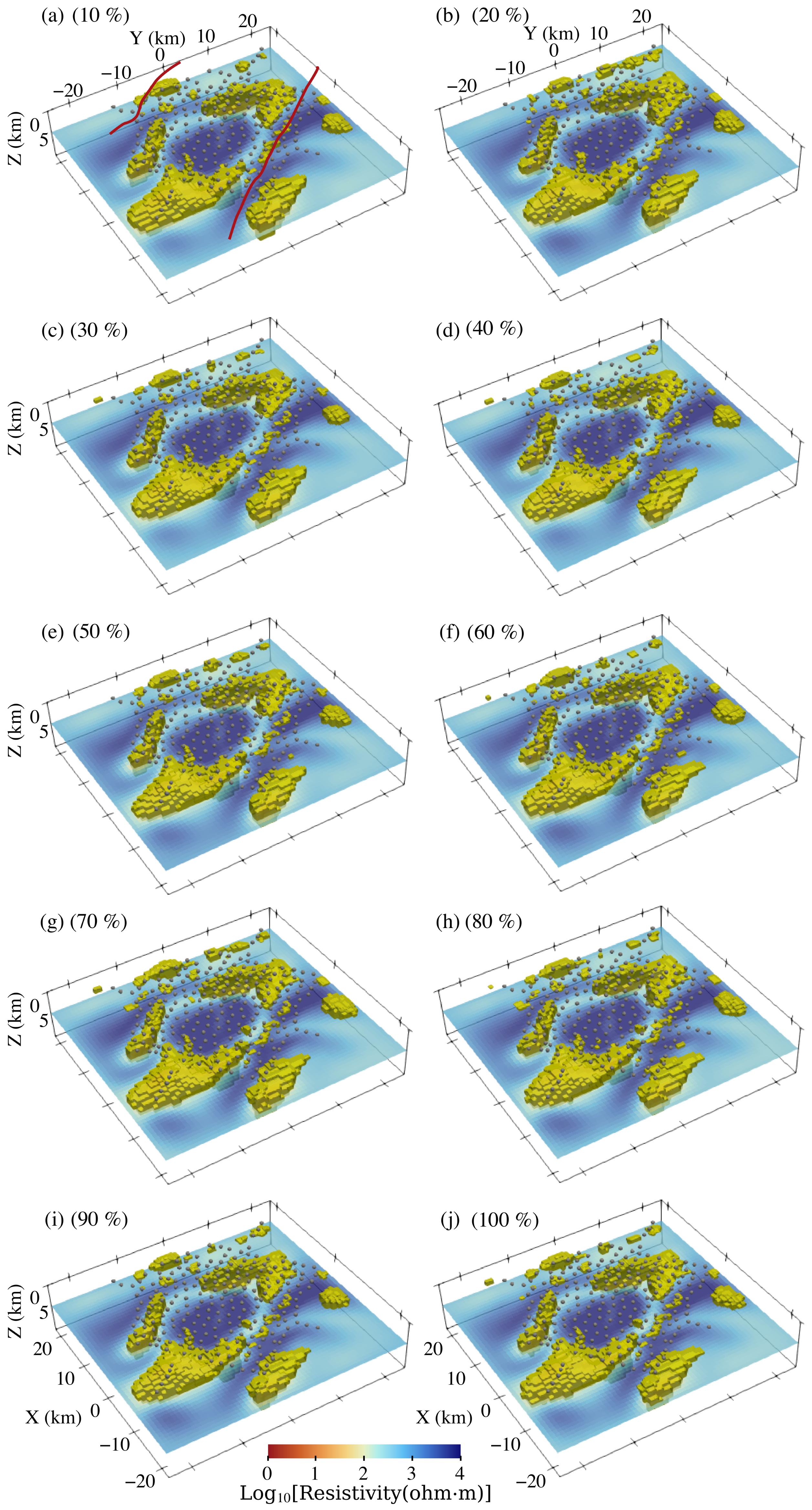
The inversion results are presented in Figure 4, with the corresponding performance metrics summarized in

Table 2. Effect of sampling ratio on inversion accuracy, convergence behavior, and computational efficiency (Akebasitao).

Sampling Ratio (%)	NRMS	Iterations	Time (h)	Peak Memory (GB)	mRMS	PCC
10	1.99	48	49.89	370.40	0.014	0.985
20	1.94	36	43.61	374.99	0.039	0.958
30	1.95	48	49.50	386.90	0.019	0.976
40	1.99	47	50.25	404.54	0.025	0.970
50	1.97	48	69.95	410.69	0.040	0.958
60	1.94	46	76.24	419.60	0.026	0.976
70	1.91	40	70.49	448.30	0.019	0.980
80	2.00	22	44.49	488.12	0.045	0.954
90	1.95	30	66.34	507.39	0.037	0.959
100	1.94	31	71.64	542.50	-	-

. The major resistive and conductive structures are consistently recovered across all sampling ratios. The dominant resistive body corresponds to the Akebasitao pluton, which exhibits relatively high resistivity characteristic of granitic intrusive rocks. In contrast, several conductive anomalies are distributed along the margins of the intrusion and within the major fault-fracture zones. These conductive features are likely associated with fractured and altered rocks related to the Darbut fault system, together with conductive ophiolitic mélanges developed along tectonic boundaries. Although the overall large-scale conductivity framework remains highly consistent across different sampling ratios, some small-scale anomalies within the fractured zones exhibit noticeable variability, reflecting the greater structural complexity and comparatively weaker resolution of these regions. Nevertheless, the mRMS values between the logarithmic resistivity models remain small (0.014–0.045), and the PCC values are consistently high (0.954–0.985), indicating that the recovered large-scale structures are highly consistent with those obtained from the full-data inversion.

From the perspective of mineral exploration, the recovered conductive anomalies are particularly significant because they may indicate hydrothermal alteration and pyrometasomatic mineralization associated with magmatic intrusion processes. Previous studies suggested that the interaction between intrusive activity and fault-controlled fluid migration played an important role in regional metallogenesis [59]. The SGN inversion successfully preserves these major conductive structures over a wide range of sampling ratios, indicating that the proposed stochastic framework retains the key geological features relevant to deep mineral exploration while also revealing the relative stability of different conductive targets within structurally complex regions.

4. Discussion

The effectiveness of the proposed SGN framework originates from two characteristics of MT inversion. First, MT datasets typically contain substantial redundancy because neighboring frequencies and stations often provide correlated constraints on the subsurface conductivity structure. Consequently, a randomly selected subset can retain much of the information contained in the full dataset. Second, MT forward modelling possesses a unique property whereby a single forward simulation for a given frequency simultaneously provides responses at all receiver locations. This property allows the line search to be performed using the complete dataset, ensuring a consistent decrease of the true objective function.

The computational performance analysis demonstrates that reducing the sampling ratio leads to substantial reductions in both memory usage and runtime. This behavior reflects the fact that the dominant computational cost in GN-based MT inversion lies in sensitivity computation, which scales approximately linearly with the number of data components. In contrast, the additional cost associated with solving the normal equations is comparatively small. For the synthetic multiblock case, the computational efficiency improves almost monotonically as the sampling ratio decreases. Although the trend is less systematic for the real-world dataset, lower sampling ratios generally lead to reduced computational cost.

From an optimization perspective, SGN can be interpreted as a stochastic approximation to the deterministic GN search direction. Because the MT inverse problem is highly nonlinear and non-convex, the deterministic GN update is not necessarily optimal and may be influenced by local curvature of the objective function. The stochastic approximation introduces perturbations into the search direction, thereby altering the optimization trajectory and leading to variability in convergence behavior across different sampling ratios.

The influence of stochasticity is also reflected in the recovered geological structures. In the Akebasitao case, the major conductive and resistive anomalies remain highly stable across different sampling ratios, whereas smaller anomalies within the fault-fracture zones exhibit noticeably stronger variability. This observation suggests that the large-scale conductive framework is strongly constrained by the MT data, while smaller-scale structures within fractured regions are comparatively less well resolved and more sensitive to inversion uncertainty owing to intrinsically higher inversion nonuniqueness.

From the perspective of mineral exploration, this distinction is particularly meaningful. The stable large-scale conductive anomalies distributed near the margins of the Akebasitao intrusion are likely to represent robust geological features associated with fault-controlled fluid migration and hydrothermal alteration. In contrast, the variability of smaller anomalies within fractured zones may reflect structural complexity, limited resolution, or the existence of multiple plausible conductivity distributions. Although uncertainty quantification is not the primary focus of this study, these results indicate that the SGN approach may provide qualitative insight into the stability and reliability of inversion-derived exploration targets.

Finally, the efficiency advantage of the SGN framework is expected to become increasingly significant for large-scale MT problems involving dense observation networks or broad frequency ranges, where sensitivity-related operations constitute a major component of the overall inversion cost. In contrast, for sparse MT datasets, the computational burden of conventional inversion is typically much lower, making stochastic subsampling largely unnecessary and potentially exacerbating the difficulties associated with limited data coverage. Future work will focus on evaluating the performance of the proposed framework under more challenging inversion settings, including anisotropic conductivity models and marine MT applications, as well as investigating adaptive sampling strategies for further improving computational efficiency.

5. Conclusions

In this study, we developed an SGN framework for large-scale 3D MT inversion by incorporating random data subsampling into sensitivity computation. By exploiting the intrinsic characteristics of MT forward modelling, the proposed method enables line search using the full-data objective function while constructing the Jacobian matrix from only a subset of data, thereby maintaining stable convergence with substantially reduced computational cost. Numerical experiments on both synthetic and real-world datasets demonstrate that the SGN method can significantly reduce runtime and memory consumption over a wide range of sampling ratios while preserving the major conductive and resistive structures recovered by conventional full-data inversion. The results further suggest that stochastic sampling may alter the optimization trajectory. Overall, the proposed SGN framework provides an efficient and scalable approach for large-scale 3D MT inversion. In addition to computational acceleration, repeated stochastic inversions may offer useful qualitative information regarding the stability of recovered geological structures, indicating potential applications in deep mineral exploration and uncertainty-oriented geophysical interpretation.

References

- Tikhonov, A. On Determining Electrical Characteristics of the Deep Layers of the Earth’s Crust. Dokl. Akad. Nauk SSSR 1950, 73, 295–297. [Google Scholar]
- Cagniard, L. Basic Theory of the Magneto-Telluric Method of Geophysical Prospecting. Geophysics 1953, 18, 605–635. [Google Scholar] [CrossRef] [Scilit]
- Chave, A.D.; Jones, A.G. The Magnetotelluric Method: Theory and Practice; Cambridge University Press: Cambridge, UK, 2012. [Google Scholar]
- Kelbert, A.; Meqbel, N.; Egbert, G.D.; Tandon, K. ModEM: A Modular System for Inversion of Electromagnetic Geophysical Data. Comput. Geosci. 2014, 66, 40–53. [Google Scholar] [CrossRef] [Scilit]
- Li, J.; Liu, J.; Ogawa, Y.; Guo, R.; Wang, X.; Wang, Y.; Zhou, K.; Xu, J. Three-Dimensional Magnetotelluric Inversion Using an Adaptive Algebraic Multi-Resolution Sampling Approach. Geophysics 2025, 90, E225–E239. [Google Scholar] [CrossRef] [Scilit]
- Wang, Y.; Liu, J.; Guo, R. Efficient Multigrid Algorithms for Three-Dimensional Electromagnetic Forward Modeling. Surv. Geophys. 2025, 46, 555–593. [Google Scholar] [CrossRef] [Scilit]
- Di, Q.; Xue, G.; Zeng, Q.; Wang, Z.; An, Z.; Lei, D. Magnetotelluric Exploration of Deep-Seated Gold Deposits in the Qingchengzi Orefield, Eastern Liaoning (China), Using a SEP System. Ore Geol. Rev. 2020, 122, 103501. [Google Scholar] [CrossRef] [Scilit]
- Shi, Y.; Xu, Y.; Yang, B.; Peng, Z.; Liu, S. Three-Dimensional Audio-Frequency Magnetotelluric Imaging of Zhuxi Copper-Tungsten Polymetallic Deposits, South China. J. Appl. Geophys. 2020, 172, 103910. [Google Scholar] [CrossRef] [Scilit]
- Liu, C.; Jing, J.e.; Jin, S.; Yin, Y.; Xie, C.; Ye, G.; Sheng, Y.; Ji, L. The Structurally-Controlled Polyphase Au Mineralization in the Southern Youjiang Basin: Insights from Magnetotelluric Imaging. Ore Geol. Rev. 2024, 169, 106090. [Google Scholar] [CrossRef] [Scilit]
- Patro, P.K. Magnetotelluric Studies for Hydrocarbon and Geothermal Resources: Examples from the Asian Region. Surv. Geophys. 2017, 38, 1005–1041. [Google Scholar] [CrossRef] [Scilit]
- Kang, Z.; Ye, G.; Jin, S.; Xie, W. Deep Thermal Source and Genesis Mechanism of Hot Dry Rock in the Jidong Region: Evidence from Magnetotelluric Array Data. Geothermics 2026, 137, 103592. [Google Scholar] [CrossRef] [Scilit]
- Patro, P.K.; Egbert, G.D. Regional Conductivity Structure of Cascadia: Preliminary Results from 3D Inversion of USArray Transportable Array Magnetotelluric Data. Geophys. Res. Lett. 2008, 35, 2008GL035326. [Google Scholar] [CrossRef] [Scilit]
- Evans, R.L.; Wannamaker, P.E.; McGary, R.S.; Elsenbeck, J. Electrical Structure of the Central Cascadia Subduction Zone: The EMSLAB Lincoln Line Revisited. Earth Planet. Sci. Lett. 2014, 402, 265–274. [Google Scholar] [CrossRef] [Scilit]
- Yang, B.; Egbert, G.D.; Kelbert, A.; Meqbel, N.M. Three-Dimensional Electrical Resistivity of the North-Central USA from EarthScope Long Period Magnetotelluric Data. Earth Planet. Sci. Lett. 2015, 422, 87–93. [Google Scholar] [CrossRef] [Scilit]
- Murphy, B.S.; Egbert, G.D. Synthesizing Seemingly Contradictory Seismic and Magnetotelluric Observations in the Southeastern United States to Image Physical Properties of the Lithosphere. Geochem. Geophys. Geosyst. 2019, 20, 2606–2625. [Google Scholar] [CrossRef] [Scilit]
- Yang, B.; Egbert, G.D.; Zhang, H.; Meqbel, N.; Hu, X. Electrical Resistivity Imaging of Continental United States from Three-Dimensional Inversion of EarthScope USArray Magnetotelluric Data. Earth Planet. Sci. Lett. 2021, 576, 117244. [Google Scholar] [CrossRef] [Scilit]
- Egbert, G.D.; Yang, B.; Bedrosian, P.A.; Key, K.; Livelybrooks, D.W.; Schultz, A.; Kelbert, A.; Parris, B. Fluid Transport and Storage in the Cascadia Forearc Influenced by Overriding Plate Lithology. Nat. Geosci. 2022, 15, 677–682. [Google Scholar] [CrossRef] [Scilit]
- Moorkamp, M.; Özaydın, S.; Selway, K.; Jones, A.G. Probing the Southern African Lithosphere with Magnetotellurics—Part I: Model Construction. J. Geophys. Res. Solid Earth 2022, 127, e2021JB023117. [Google Scholar] [CrossRef] [Scilit]
- Munch, F.D.; Grayver, A. Multi-Scale Imaging of 3-D Electrical Conductivity Structure under the Contiguous US Constrains Lateral Variations in the Upper Mantle Water Content. Earth Planet. Sci. Lett. 2023, 602, 117939. [Google Scholar] [CrossRef] [Scilit]
- Neukirch, M.; Minakov, A.; Smirnov, M.; Gaina, C.; Munteanu, I.; Panea, I. Electrical Resistivity Imaging of the Northeast Carpathian Volcanic Arc with 3-D Magnetotellurics Reveals Shallow Hydrothermal System. J. Geophys. Res. Solid Earth 2024, 129, e2023JB028230. [Google Scholar] [CrossRef] [Scilit]
- Montiel-Álvarez, A.M.; Hübert, J.; Whaler, K.; Beggan, C.D.; Kiyan, D.; Hogg, C. The First Three-Dimensional Electrical Resistivity Model of the Lithosphere beneath Britain. J. Geophys. Res. Solid Earth 2025, 130, e2025JB031813. [Google Scholar] [CrossRef] [Scilit]
- Wang, J.; Zhang, L.; Peng, W.; Zhu, D.; Qi, C.; Chang, J. Deep Electrical Structure and Tectonic Implications of the Yinchuan Basin and Surrounding Areas. Tectonophysics 2026, 929, 231140. [Google Scholar] [CrossRef] [Scilit]
- Grayver, A.V. Parallel Three-Dimensional Magnetotelluric Inversion Using Adaptive Finite-Element Method. Part I: Theory and Synthetic Study. Geophys. J. Int. 2015, 202, 584–603. [Google Scholar] [CrossRef] [Scilit]
- Feng, D.; Su, X.; Wang, X.; Wang, X. A Modified Total Variation Regularization Approach Based on the Gauss–Newton Algorithm and Split Bregman Iteration for Magnetotelluric Inversion. J. Appl. Geophys. 2020, 178, 104073. [Google Scholar] [CrossRef] [Scilit]
- Nádasi, E.; Gribenko, A.V.; Zhdanov, M.S. Large-Scale Inversion of Magnetotelluric Data Using Regularized Gauss–Newton Method in the Data Space. Pure Appl. Geophys. 2022, 179, 3785–3806. [Google Scholar]
- Zhou, J.; Han, B.; Junge, A.; Hu, X.; Xiao, T.; Long, Z.; Bai, N. Effective Gauss–Newton Inversion for 3D Magnetotelluric Data with Arbitrarily Anisotropic Conductivities. Phys. Earth Planet. Inter. 2025, 369, 107465. [Google Scholar] [CrossRef] [Scilit]
- Constable, S.C.; Parker, R.L.; Constable, C.G. Occam’s Inversion: A Practical Algorithm for Generating Smooth Models from Electromagnetic Sounding Data. Geophysics 1987, 52, 289–300. [Google Scholar] [CrossRef] [Scilit]
- Siripunvaraporn, W.; Egbert, G.; Lenbury, Y.; Uyeshima, M. Three-Dimensional Magnetotelluric Inversion: Data-Space Method. Phys. Earth Planet. Inter. 2005, 150, 3–14. [Google Scholar] [CrossRef] [Scilit]
- Key, K. MARE2DEM: A 2-D Inversion Code for Controlled-Source Electromagnetic and Magnetotelluric Data. Geophys. J. Int. 2016, 207, 571–588. [Google Scholar] [CrossRef] [Scilit]
- Egbert, G.D.; Kelbert, A. Computational Recipes for Electromagnetic Inverse Problems. Geophys. J. Int. 2012, 189, 251–267. [Google Scholar] [CrossRef] [Scilit]
- Oldenburg, D.W. Practical Strategies for the Solution of Large-Scale Electromagnetic Inverse Problems. Radio Sci. 1994, 29, 1081–1099. [Google Scholar] [CrossRef] [Scilit]
- Avdeev, D.; Avdeeva, A. 3D Magnetotelluric Inversion Using a Limited-Memory Quasi-Newton Optimization. Geophysics 2009, 74, F45–F57. [Google Scholar] [CrossRef] [Scilit]
- Chen, H.; Ren, Z.; Tang, J. Magnetotelluric Adaptive Inversion Using Multi-resolution Tetrahedral Grids: Application to the North China Craton. J. Geophys. Res. Solid Earth 2025, 130. [Google Scholar] [CrossRef] [Scilit]
- Cockett, R.; Kang, S.; Heagy, L.J.; Pidlisecky, A.; Oldenburg, D.W. SimPEG: An Open Source Framework for Simulation and Gradient Based Parameter Estimation in Geophysical Applications. Comput. Geosci. 2015, 85, 142–154. [Google Scholar] [CrossRef] [Scilit]
- Ruder, S. An Overview of Gradient Descent Optimization Algorithms. arXiv 2017, arXiv:1609.04747. [Google Scholar]
- Duchi, J.; Hazan, E.; Singer, Y. Adaptive Subgradient Methods for Online Learning and Stochastic Optimization. J. Mach. Learn. Res. 2011, 12, 2121–2159. [Google Scholar]
- Kingma, D.P.; Ba, J. Adam: A Method for Stochastic Optimization. arXiv 2015, arXiv:1412.6980. [Google Scholar]
- Dozat, T. Incorporating Nesterov Momentum into Adam. In Proceedings of the Fourth International Conference on Learning Representations; ICLR: San Juan, Puerto Rico, 2016; pp. 1–4. [Google Scholar]
- Phuong, T.T.; Phong, L.T. On the Convergence Proof of AMSGrad and a New Version. IEEE Access 2019, 7, 61706–61716. [Google Scholar] [CrossRef] [Scilit]
- Liu, L.; Jiang, H.; He, P.; Chen, W.; Liu, X.; Gao, J.; Han, J. On the Variance of the Adaptive Learning Rate and Beyond. arXiv 2020, arXiv:1908.03265. [Google Scholar]
- Bellavia, S.; Krejic, N.; Jerinkic, N.K. Subsampled Inexact Newton Methods for Minimizing Large Sums of Convex Functions. arXiv 2018, arXiv:1811.05730. [Google Scholar]
- Bollapragada, R.; Byrd, R.H.; Nocedal, J. Exact and Inexact Subsampled Newton Methods for Optimization. IMA J. Numer. Anal. 2019, 39, 545–578. [Google Scholar] [CrossRef] [Scilit]
- Berahas, A.S.; Bollapragada, R.; Nocedal, J. An Investigation of Newton-Sketch and Subsampled Newton Methods. Optim. Methods Softw. 2020, 35, 661–680. [Google Scholar] [CrossRef] [Scilit]
- Tran-Dinh, Q.; Pham, N.H.; Nguyen, L.M. Stochastic Gauss–Newton Algorithms for Nonconvex Compositional Optimization. In Proceedings of the 37th International Conference on Machine Learning; PMLR: New York, NY, USA, 2020. [Google Scholar]
- Bergou, E.; Chada, N.K.; Diouane, Y. A Stochastic Iteratively Regularized Gauss–Newton Method. Inverse Probl. 2025, 41, 15005. [Google Scholar] [CrossRef] [Scilit]
- Van Leeuwen, T.; Aravkin, A.Y.; Herrmann, F.J. Seismic Waveform Inversion by Stochastic Optimization. Int. J. Geophys. 2011, 2011, 689041. [Google Scholar] [CrossRef] [Scilit]
- Martin, J.; Wilcox, L.C.; Burstedde, C.; Ghattas, O. A Stochastic Newton MCMC Method for Large-Scale Statistical Inverse Problems with Application to Seismic Inversion. SIAM J. Sci. Comput. 2012, 34, A1461–A1487. [Google Scholar] [CrossRef] [Scilit]
- Yang, D.; Oldenburg, D.W.; Haber, E. 3-D Inversion of Airborne Electromagnetic Data Parallelized and Accelerated by Local Mesh and Adaptive Soundings. Geophys. J. Int. 2014, 196, 1492–1507. [Google Scholar] [CrossRef] [Scilit]
- Yang, D.; Oldenburg, D.W. Survey Decomposition: A Scalable Framework for 3D Controlled-Source Electromagnetic Inversion. Geophysics 2016, 81, E69–E87. [Google Scholar] [CrossRef] [Scilit]
- Ren, X.; Lai, M.; Wang, L.; Yin, C.; Liu, Y.; Su, Y.; Zhang, B.; Ben, F.; Huang, W. A Fast 3-D Inversion for Airborne EM Data Using Pre-Conditioned Stochastic Gradient Descent. Geophys. J. Int. 2023, 234, 737–754. [Google Scholar] [CrossRef] [Scilit]
- Ren, X.; Lai, M.; Wang, L.; Yin, C.; Liu, Y.; Su, Y.; Zhang, B. Footprint-Driven Stochastic Approximation Inversion for Time-Domain Airborne Electromagnetic Data. Geophysics 2024, 90, WA17–WA29. [Google Scholar] [CrossRef] [Scilit]
- Su, Y.; Ren, X.; Yin, C.; Wang, L.; Liu, Y.; Zhang, B.; Wang, L. Multiscale 3-D Stochastic Inversion of Frequency-Domain Airborne Electromagnetic Data. Remote Sens. 2024, 16, 3070. [Google Scholar] [CrossRef] [Scilit]
- Donoho, D.L. Compressed sensing. IEEE Trans. Inf. Theory 2006, 52, 1289–1306. [Google Scholar] [CrossRef] [Scilit]
- Levenberg, K. A Method for the Solution of Certain Non-Linear Problems in Least Squares. Q. Appl. Math. 1944, 2, 164–168. [Google Scholar] [CrossRef] [Scilit]
- Marquardt, D.W. An Algorithm for Least-Squares Estimation of Nonlinear Parameters. J. Soc. Ind. Appl. Math. 1963, 11, 431–441. [Google Scholar] [CrossRef] [Scilit]
- Nocedal, J.; Wright, S.J. Numerical Optimization, 2nd ed.; Springer Series in Operations Research; Springer: New York, NY, USA, 2006. [Google Scholar]
- Liu, L.; Yang, B.; Zhang, Y.; Xu, Y.; Peng, Z.; Yang, D. Calculating Sensitivity or Gradient for Geophysical Inverse Problems Using Automatic and Implicit Differentiation. Comput. Geosci. 2024, 193, 105736. [Google Scholar] [CrossRef] [Scilit]
- Curry, M. ModEM-Examples: GitHub Repository. 2025. Available online: https://github.com/magnetotellurics/ModEM-Examples (accessed on 2 January 2026).
- Yang, B.; Zhang, A.; Zhang, S.; Liu, Y.; Zhang, S.; Li, Y.; Xu, Y.; Wang, Q. Three-dimensional audio-frequency magnetotelluric imaging of Akebasitao granitic intrusions in Western Junggar, NW China. J. Appl. Geophys. 2016, 135, 288–296. [Google Scholar] [CrossRef] [Scilit]
Disclaimer/Publisher’s Note: The statements, opinions and data contained in all publications are solely those of the individual author(s) and contributor(s) and not of MDPI and/or the editor(s). MDPI and/or the editor(s) disclaim responsibility for any injury to people or property resulting from any ideas, methods, instructions or products referred to in the content. |
© 2026 by the authors. Licensee MDPI, Basel, Switzerland. This article is an open access article distributed under the terms and conditions of the Creative Commons Attribution (CC BY) license.