


Abstract
The performance of remote sensing-based mineral alteration extraction is significantly restricted in the vegetation area. Spectral unmixing is one of the effective methods to address the vegetation problem during mineral alteration extraction. However, the spectral curves of different tree species vary a lot; if multiple tree species are regarded as a whole during the spectral unmixing stage, the proportions of vegetation would be estimated with more errors. The purpose of this study was to verify the effects of dominant tree species classification on spectral unmixing and reconstruction, and to apply the proposed method to the mineral alteration extraction practice. To accomplish this, the Shabaosi gold deposit region in Mohe City, China, with an area of 650 km2, was selected as the study area. Firstly, reference spectral curves, GaoFen-1/6 (GF-1/6) satellite imageries, ZiYuan-1F (ZY-1F) satellite imageries, Sentinel-1B satellite synthetic aperture radar (SAR) data, the ALOS digital elevation model (DEM), and sub-compartment dominant tree species data were collected; subsequently, simulated mixed-pixel reflectance images of ZY-1F, reflectance images of GF-1/6, ZY-1F, backscattering data of Sentinel-1B, slope, aspect, and 5484 tree species samples were derived from the collected data. Secondly, to verify the effect of dominant tree species classification on mineral alteration extraction, the reference spectra of pine, oak, goethite, and kaolinite were used to construct a simulated ZY-1F mixed-pixel image, and spectral unmixing and reconstruction experiments were conducted. Thirdly, fourteen independent variables were selected from the derived data, five dominant tree species classification models were trained and tested using tree species samples via the ResNet50 algorithm, and the pine- and birch-dominated parts were segmented from the ZY-1F images. Fourthly, minimum noise fraction (MNF), pixel purity index (PPI), n-dimensional visualizer auto-clustering, and spectral angle mapper (SAM) methods were separately applied to the pine- and birch-dominated parts of ZY-1F images to extract and identify endmembers; subsequently, the fully constrained least squares (FCLS) and linear spectral unmixing (LSU) methods were separately applied to the pine- and birch-dominated parts to estimate endmember proportions and generate spectrally reconstructed ZY-1F images. Fifthly, the pine- and birch-dominated parts of spectrally reconstructed ZY-1F images were mosaiced, and the SAM was utilized to extract mineral alteration in the study area. The result showed that in the spectral unmixing and reconstruction experiment, the spectral reconstruction error declined from 0.0594 (simulated ZY-1F image without segmentation) to 0.0292 and 0.0388 (simulated ZY-1F image that was segmented by pine- and oak-dominated parts), suggesting that dominant tree species classification could improve the accuracy of spectral unmixing and reconstruction and help obtain a more reliable mineral alteration extraction result. In the study area, the tested overall accuracies (OA) and Kappa coefficients of the five dominant tree species classification models were 0.75 ± 0.03 and 0.50 ± 0.05, respectively, suggesting that conducting dominant tree species classification was feasible in dense vegetation areas and could facilitate mineral alteration extraction. After segmenting the ZY-1F image by pine- and birch-dominated parts and spectral reconstruction, eight main types of alteration, including kaolinite, vesuvianite, montmorillonite, rutile, limonite, mica, sphalerite, and quartz, were identified, and nine mineral alteration areas (MA) were delineated accordingly.
1. Introduction
Mineral resources are essential to industrialization [1] and sustainable development; there is an urgent call for the primary production increase of many mineral resources [2]. The increasing demand and heterogeneous distribution of critical metal mineral resources [3] are jointly shedding more pressure on mineral prospectivity mapping (MPM), including the 2-dimensional (2D) MPM for new mineralization sites in regional scale [4] and the 3-dimensional (3D) MPM for deeply buried ore bodies in mining district scale [5]. Geological, geophysical, and drilling data are constantly vital in the 3D MPM [6,7,8,9,10], while during the 2D MPM, geological, geophysical, geochemical, and remote sensing data are commonly necessary [11,12,13,14,15]. Being easily accessible, spatially extended, and spectrally wide, the remote sensing data could be significantly assistive during the early stage of mineral exploration [16] and has been introduced to regional 2D MPM since the 1970s [17].
Remote sensing data, covering the visible and near-infrared bands (VNIR) and shortwave-infrared bands (SWIR), plays a role as the basis of visually geological units’ interpretation and quantitative mineral alteration extraction. The spectral intensity of solar radiation reflected by natural surface is influenced by the physical and chemical properties of the materials [18]; they tend to show particular spectral curves and absorption (or reflectance) at some fixed wavelengths [19] and are advantageous to the fundamental mineral alteration extraction methods, including band ratio, principal component analysis (PCA), and spectral angle mapper (SAM). Band ratio is usually applied to the multi-spectral remote sensing imagery and could highlight the trace of iron oxide/hydroxide-class and hydroxyl-bearing minerals [18] by the ratio between reflectance bands and absorption bands. Ousmanou et al. (2024) used the band ratio algorithm to extract iron oxide, clay, and carbonate minerals from Landsat-9 OLI and advanced spaceborne thermal emission and reflection radiometer (ASTER) data in the Banyo area, Cameroon [20]. Madeleine et al. (2025) also used the Landsat-9 OLI data and the band ratio algorithm during the extraction of iron oxide/hydroxide and hydroxyl minerals in the Bonako area, Cameroon [21]. The PCA approach is also designed to deal with multi-spectral remote sensing imagery. PCA is a multi-dimensional data compression algorithm that could remove co-linear relationships between spectral bands [22]; this approach is generally performed on four typical reflectance/absorption bands, and the principal component (PC) holding indicative eigenvector loadings could represent the intensity of iron oxide/hydroxide-class and hydroxyl-bearing minerals [23]. Wanduku et al. (2021) used the Landsat-7 ETM+, ASTER data, and PCA method to identify patterns related to clay and iron alteration in part of the Malumfashi Schist Belt, Nigeria [24]. Orynbassarova et al. (2025) also adopted the PCA algorithm to the Landsat-8 OLI and ASTER data, and distributions of iron oxides/hydroxides and clay minerals were obtained in the Aktogay copper deposit area, Kazakhstan [25]. The SAM method is mainly suitable to hyper-spectral imagery, and it treats every pixel as a vector in the n-dimensional (n-D) space and calculates the spectral angle between the pixel spectra vector and the reference spectrum vector; the spectral angle relies on overall spectral compatibility rather than individual diagnostic absorption feature [26,27], making it robust to images sensed from different dates and solar radiation conditions. Hegab et al. (2024) calculated the spectral angle between the ASTER image and reference spectra and identified sericite, kaolinite, calcite, illite, hematite, montmorillonite, chlorite, alunite, and epidote in the Elkharaza-Dara Area, Egypt [28]. Zhang et al. (2024) also applied SAM to the GaoFen-5 (GF-5) satellite hyper-spectral image, and albite, biotite, chlorite, hornblende, and muscovite clues were spotted in the Lala region, Sichuan, China [29].
Remote sensing imageries authentically provide vivid surface pictures and abundant mineral information in bedrock-exposed regions, for example, the East Junggar in Xinjiang, China [30]. However, due to the tree canopy and the weak penetrability of the VNIR and SWIR bands, the mineral alteration extraction ability is significantly weakened or eliminated in the vegetation area. Measures have been taken to address the vegetation problem during mineral alteration extraction, including masking, directed principal component analysis (DPCA), soil and vegetation spectral coupling difference (SVSCD), spectral unmixing, and integrated methods that are combined with normalized difference vegetation index (NDVI)-based image segmentation and spectral unmixing. The masking method simply removes dense vegetation pixels and results in numerous blank areas or voids in the imagery. Unlike the conventional PCA method, the DPCA method conducts PCA transform on two band ratio images; one of the ratio images highlights mineral alteration information, and the other ratio image highlights vegetation information. Similar to the PCA method, the output principal component (PC) holding indicative eigenvector loadings could represent the intensity of iron oxide/hydroxide-class and hydroxyl-bearing minerals [31,32,33]. The SVSCD method seeks to suppress vegetation information via the difference between three band couples, with every band couple sharing similar vegetation spectral reflectance and different soil/mineral spectral reflectance; subsequently, the PCA is performed on these three band couple difference images, and the PC1 and PC2 would be plotted on a scatter diagram; and finally, the abnormal pixels are selected and identified via spectral feature fitting (SFF) [34]. The spectral unmixing method (i.e., mixed-pixel decomposition) is constantly performed on hyperspectral images; it considers the spectral reflectance of a pixel as the integrated spectral reflectance of different ground substances (i.e., endmembers) within this particular pixel. After the spectral curves of endmembers (collected directly from the spectral dataset or extracted from the image) are provided, various algorithms are developed to estimate the proportions of endmembers within a pixel, including matched filtering (MF), mixture tuned matched filtering (MTMF), constrained energy minimization (CEM), adaptive coherence estimator (ACE), orthogonal subspace projection (OSP), and fully constrained least squares (FCLS) [35,36,37,38,39]. After the endmember proportions are estimated, researchers tend to regard the estimated proportion of the target mineral as the mineral intensity [40,41].
In contrast to the inconvenience of mineral alteration extraction in the vegetation area, the tree species classification verifies the efficiency and reliability of remote sensing technology. Researchers have applied various algorithms to diverse data to obtain the regional distribution of tree species. Raczko et al. (2017) collected airborne hyperspectral data in Szklarska Poręba area, Poland, and compared the performances of support vector machine (SVM), random forest (RF), and artificial neural networks (ANN) algorithm on the classification of spruce, larch, alder, beech, and birch, and the result showed that ANN possessed the highest overall accuracy (OA) of 77% [42]. Knauer et al. (2019) introduced a convolutional neural network (CNN) algorithm to tree species classification in Saxony Anhalt and Thuringia, Germany, where airborne hyperspectral data were obtained, and the OA turned out to be 73% [43]. Liu et al. (2023) obtained true color composite orthophotos and LiDAR point clouds data in the Gaofeng Forest Farm, Nanning, China, and combined the ResNet50 and PointMLP architectures to classify eucalyptus and Chinese fir; an OA of 98.52% was recorded [44].
Considering the mineral alteration extraction and tree species classification methods mentioned above, it would be better to improve the spectral unmixing process in two aspects. Firstly, spectral curves of different tree species are not completely identical, especially the reflectance within 760~1300 nanometers (nm) [45]. During the spectral unmixing stage, the proportions of tree species with higher NIR reflectance tend to be overestimated, and the proportions of tree species with lower NIR reflectance tend to be underestimated, so image segmentation is proposed before the spectral unmixing, and segmentation by tree species is more recommended than by vegetation density. Secondly, in bedrock-exposed regions, the estimated proportion of minerals could be equivalent to the intensity of mineral alteration. However, this hypothesis is not appropriate in the vegetation area; assuming Pixel A is a covered by 80% vegetation and 20% soil (kaolinite accounts for 50% of the soil), and Pixel B is a covered by 20% vegetation and 80% soil (kaolinite accounts for 10% of the soil), the calculated proportion of kaolinite in Pixel A might be lower than in Pixel B, which is opposite to the ground truth that the soil kaolinite content is higher in Pixel A than in Pixel B. It is better to reduce the spectral effects of vegetation and reconstruct the ground spectrum in each pixel, and then extract the mineral alteration intensity via the regular methods that are used in bedrock exposure regions.
As the spectral difference between tree species would pull down the accuracy of spectral unmixing, this study proposed a new methodological workflow, which involved introducing dominant tree species classification to the mineral alteration extraction in the vegetation area. The objective of this study was to find out the effects of dominant tree species classification on mineral alteration, and an experiment and a practice were both implemented. In the experiment stage, a simulated ZiYuan-1F satellite (ZY-1F) hyperspectral mixed-pixel image was constructed, and the simulated image was preprocessed with three separate strategies, including no segmentation, segmentation by tree species, and segmentation by NDVI. Then, images with different processing strategies were spectrally unmixed and reconstructed, and their spectral reconstruction errors were used to verify whether dominant tree species classification could theoretically improve the accuracy of spectral unmixing and reconstruction in the vegetation area. In the practice stage, the Shabaosi gold deposit region in China was selected as the study area, and the sub-compartment data with dominant tree species, the GaoFen-1/6 satellite (GF-1/6) multi-spectral image, the ZY-1F hyperspectral image, Sentinel-1B synthetic aperture radar (SAR) data, and the digital elevation model (DEM) were collected. The ZY-1F image was preprocessed with two separate strategies, including no segmentation and segmentation by tree species via the ResNet50 algorithm, and images with different processing strategies were spectrally unmixed and reconstructed. Then, the SAM method was applied to extract mineral alteration from the spectrally reconstructed ZY-1F images with different processing strategies, and their mineral alteration distribution results were compared with stream sediment Au content to verify whether dominant tree species classification could practically improve the reliability of mineral alteration extraction in the vegetation area.
2. Study Area
The Shabaosi gold deposit region in Mohe City, Heilongjiang Province, China, was selected as the study area; it is a 650 km2 hilly region located in the north of the Greater Khingan Range (Figure 1a). The coldest and hottest months are January and July, respectively, and precipitation is primarily concentrated from July to August. The elevation ranges from 300 m to 850 m, and slopes are mostly less than 30 degrees. Due to environmental preservation policies and moderate slope, most of the study area is unexploited and covered by dense forest; the tree species are mainly pine and birch, and tend to grow in clusters, which is suitable for dominant tree species classification (Figure 1b). Geological units consist of lower washland, higher washland, lower Cretaceous Ganhe formation, middle Jurassic Mohe formation, Ershierzhan formation, Xiufeng formation, lower Devonian Niqiuhe formation, Ordovician-Silurian Jixianggou formation, Meso-Neo-Proterozoic Xinghuadukou formation, early Cretaceous granite porphyry, granite, and diorite, and Ordovician monzonitic granite, granodiorite, and diorite (Figure 1c). The Shabaosi large gold deposit is located in the middle-southwest of the study area, and is controlled by faults and formed by the magma hydrothermal fluid during the early Cretaceous [46,47].
Figure 1.
(a) Location in Northeastern China, (b) true color image from Landsat 8 OLI in August, and (c) regional geological map of the study area.
3. Data and Methods
Figure 2 shows the workflow of this study, comprising five main parts: data acquisition, spectral unmixing and reconstruction experiment, dominant tree species classification, spectral unmixing and reconstruction, and mineral alteration extraction.
Figure 2.
Workflow of the study.
3.1. Data Acquisition
The original data, including reference spectral curves, GF-1/6 Level-1A image, ZY-1F Level-1A image, Sentinel-1B IW GRDH image, DEM, sub-compartment dominant tree species data, and Au content map of stream sediment, were acquired from relevant institutions, and then, various measures were taken to obtain derived data from the original data (Table 1).
Table 1.
Data list.
3.1.1. Simulated ZY-1F Image
The study area was mainly covered by pine and birch; the simulated image constructed using pine, birch, goethite, and kaolinite reference spectral curves would be preferred, but birch was absent from the USGS spectral library, so it was replaced by oak, which possessed an evident NIR reflectance difference with pine. A simulated ZY-1F mixed-pixel reflectance image (200-row, 400-column, 162-band) (Table 1) was constructed using pine, oak, goethite, and kaolinite reference spectral curves from the USGS spectral library. In the simulated ZY-1F image, the left part (200-row, 200-column, 162-band) is composed of pine, goethite, and kaolinite, and the right part (200-row, 200-column, 162-band) is composed of oak, goethite, and kaolinite. To construct the simulated ZY-1F image, firstly, the reference spectral curves of pine, oak, goethite, and kaolinite were spectrally resampled to 162 bands (4 limbic bands were removed from the 166 bands of ZY-1F) to approximate the real ZY-1F image. Secondly, a 200-row 200-column matrix was constructed; its values ranged from 1 to 200, and the lowest value was at the upper-left part, while the highest value was at the lower-right part (Figure 3). Thirdly, in the left part of the simulated ZY-1F image, the proportions of pine, goethite, and kaolinite endmembers were assigned:
where M refers to the 200-row 200-column matrix, Ppine refers to the spatial proportion distribution of pine endmember, which is also a 200-row 200-column matrix, Pgoethite refers to the spatial proportion distribution of goethite endmember, Pkaolinite refers to the spatial proportion distribution of kaolinite endmember, v() refers to an operator which flips the matrix vertically, and vh() refers to an operator which flips the matrix both vertically and horizontally. Fourthly, the left part of the simulated ZY-1F image was generated:
where the Ri refers to the simulated mixed-pixel reflectance matrix at band i (i ranges from 1 to 162), Ripine refers to the reference pine reflectance at band i, Rigoethite refers to the reference goethite reflectance at band i, and Rikaolinite refers to the reference kaolinite reflectance at band i. Then, the left part of the simulated ZY-1F image was constructed by the stack from R1 to R162. Fifthly, repeat Step 3 and Step 4, and replace the pine endmember with the oak endmember; then, the right part of the simulated ZY-1F image was constructed. Sixthly, the left and right parts were mosaiced to construct the simulated ZY-1F image.
Figure 3.
Matrix used for the construction of the simulated ZY-1F mixed-pixel reflectance image.
3.1.2. Optical Reflectance Image
To obtain ground reflectance images of GF-1, GF-6, and ZY-1F (Table 1), image fusion, radiometric calibration, atmospheric correction, orthorectification, and geometric registration were performed using the ENVI5.3 software. Fusion was conducted on GF-1/6 via the “nearest neighbor diffuse (NNDiffuse)” algorithm [48], and the parameters were default. Calibration was conducted on GF-1/6 and ZY-1F through algebra with gain and bias, which were built into ENVI5.3. Atmospheric correction was conducted via the “fast line-of-sight atmospheric analysis of spectral hypercubes (FLAASH)” algorithm [49]. For GF-1/6, the ground elevation was set as 0.50 km, the atmospheric model was set as sub-arctic summer, water retrieval was set as no, the aerosol model was set as rural, the aerosol retrieval method was set as none, and initial visibility was set as 40 km; for ZY-1F, the ground elevation was also set as 0.50 km, the atmospheric model was set as sub-arctic summer, water retrieval was set as yes, water absorption feature was set as 1135 nm, the aerosol model was set as rural, the aerosol retrieval method was set as 2-band (K-T), initial visibility was set as 40 km, spectral polishing was set as yes, the polishing sampling width was set as 9, and wavelength recalibration was set as no. Orthorectification was conducted on GF-1/6 and ZY-1F using ALOS DEM via the “RPC orthorectification workflow” tool. Registration was conducted via ground control points (GCPs), rational polynomial coefficients (RPCs), and the reference digital orthophoto map (DOM) via the “image registration workflow” tool. For GF-1/6, the reference DOM was from the Harbin center for integrated natural resources survey; for ZY-1F, the reference DOM was the Landsat-8 OLI image. The image resampling methods in this study were all set to cubic convolution.
3.1.3. Radar Backscattering Image
To obtain the radar backscattering image (Table 1), the SNAP12.0.0 software was utilized to process the VV and VH bands of Sentinel-1B IW GRDH data on 9 June 2019 and 7 October 2019, respectively. Firstly, the “apply orbit file” tool was used to assign precise orbit parameters to the intensity data. Secondly, the “S-1 thermal noise removal” tool was used to reduce the thermal noise in the intensity data. Thirdly, the “calibrate” tool was performed on the intensity data to obtain the linear backscattering data (Sigma0). Fourthly, the “single product speckle filter” tool was applied to reduce interferometric noise in the backscattering data. Fifthly, the “range Doppler terrain correction” tool was introduced to conduct terrain correction and assign geographic coordinates to image pixels.
3.1.4. Aspect and Slope
Aspect and slope data (Table 1) were built based on the 12.5 m-resolution ALOS DEM. The “aspect” tool in ArcGIS10.2 software was directly utilized to generate aspect; the primary result ranged from 0 to 360 and was divided by 360 to be normalized to 0~1. The “slope” tool was also applied to obtain the primary slope result and was also normalized to 0~1 via the ratio with 90.
3.1.5. Scene Samples for Dominant Tree Species Classification
Fourteen variables were utilized for dominant tree species classification, and they were spatially resampled to 2 m and stacked as one dataset, including four reflectance bands of GF-1 on 12 October 2024, four reflectance bands of GF-6 on 23 June 2024, VV/VH backscattering bands of Sentinel-1B on 9 June 2019 and 7 October 2019, aspect, and slope (Table 1). Firstly, the vector data of sub-compartment dominant tree species was converted to raster data, and the pixel values within sub-compartments of pine and birch were set as 1 and 2, respectively. Secondly, in the smallest rectangle that covered the study area, a n-row n-column scene (n is preliminarily set as 11, 31, 51, 71, and 91) started to jump from the (n − 1)/2 + 1-th row and (n − 1)/2 + 1-th column with a step length of 300 pixels for pine samples (200 pixels for birch samples); if pixels belonging to pine (or birch) exceeds n × n × 0.77, then the (n − 1)/2 + 1-row (n − 1)/2 + 1-column 14-band scene, with other 3 more scenes (the left–right flipped, up–down flipped, and left–right–up–down flipped scenes of this particular scene), would be extracted as the samples for pine (or birch), and the corresponding labels would be set as pine (or birch). Thirdly, the pine and birch samples were divided into five folds and were used to train and test tree classification models via the ResNet50 algorithm; the model performance, sample quantity, and spatial resolution of tree classification results were jointly considered to determine the final size of scene samples.
3.2. Spectral Unmixing and Reconstruction Experiment
This experiment was designed to find out whether dominant tree species classification could improve the performance of spectral unmixing and reconstruction and was conducted via ENVI5.3. Firstly, three separate preprocessing strategies were applied to the simulated ZY-1F image, including no segmentation (SimuImg #0), segmentation by tree species (the simulated ZY-1F image were segmented into the pine-part on the left (SimuImg #1) and the oak-part on the right (SimuImg #2)), and segmentation by NDVI (the simulated ZY-1F image were segmented into the no-vegetation part where NDVI was less than 0.2 (SimuImg #3) and the vegetation part where NDVI was greater than 0.2 (SimuImg #4)). Secondly, minimum noise fraction (MNF) was performed on Image #0 via the “forward MNF estimate noise statistics” tool. Thirdly, the pixel purity index (PPI) was calculated from the first 5 bands of MNF data via the “PPI new output” tool. Fourthly, the PPI (greater than 30) and the first 5 bands of MNF data were input into the “n-dimensional visualizer auto cluster” tool, and the endmembers and their spectral curves were automatically extracted and generated. Fifthly, the reference spectral curves were collected from the USGS library, and the “spectral analyst” tool and SAM algorithm were utilized to find out the most likely type of endmembers. Sixthly, the fully constrained least squares algorithm (FCLS) was used to estimate the proportions of endmembers, and could be accomplished by the “FCLS spectral unmixing” tool. Seventhly, according to the linear spectral unmixing (LSU) model, the vegetation endmembers were removed from SimuImg #0, and pixels were spectrally reconstructed. Two spectrally reconstructed images could be generated in Step 7; one was generated according to the true endmember spectral curves and proportions (namely, SimuImg #0_1), while the other was generated according to the estimated endmember spectral curves and proportions (namely, SimuImg #0_2):
where Rinew refers to spectrally reconstructed reflectance at band i, which would be set to 0 if its value was less than 0, Rioriginal refers to the original reflectance at band i, v refers to the number of vegetation endmembers, n refers to the total quantity of vegetation endmembers, Riv refers to the reflectance of the v-th vegetation endmember at band i, and Wv refers to the spatial proportion distribution of the v-th vegetation endmember. Eighthly, the spectral unmixing and reconstruction errors of band 1~162 between SimuImg #0_1 and SimuImg #0_2 were calculated:
where Ei refers to the spectral unmixing and reconstruction error of band i, abs() refers to the operator which calculates the absolute value, Ri0_1 refers to the spectrally reconstructed band i data according to the true endmember spectral curves and proportions, Ri0_2 refers to the spectrally reconstructed band i data according to the estimated endmember spectral curves and proportions, E refers to the spectrally averaged error, ei refers to the spatially averaged error of band i, and mean() refers to the operator which calculates the mean value. Ninthly, repeat Step 2~8 and calculate the spectral unmixing and reconstruction error of SimuImg #1~#4. Tenthly, the errors of SimuImg #0~#4 were compared to see whether the proposed dominant tree species classification could improve the performance of spectral unmixing and reconstruction, which could be verified by the lower errors of SimuImg #1 and #2 compared to SimuImg #0, #3, and #4.
3.3. Dominant Tree Species Classification
During dominant tree species classification, the model training and testing were performed using a 5-fold cross strategy; the ResNet50 architecture (Figure 4) with pretrained parameters was applied, and a computer with a RTX4060 8G-memory GPU (manufactured by NVIDIA, Santa Clara, CA, USA) and Python 3.11 were utilized. Firstly, during training, pine and birch samples were input into the model, the batch size was set as 8, the max epoch was 30, the initial learning rate was 0.01, and the learning rate was reduced by 0.1 times every 10 epochs; five models would be finally trained according to the 5-fold cross strategy, namely, Model #1~#5. Secondly, in the testing stage, the previous training samples and testing samples were classified by the five trained models, and a confusion matrix was applied to calculate the user’s accuracy (UA), producer’s accuracy (PA), overall accuracy (OA), and Kappa coefficient (Table 2). Thirdly, after training and testing, the stacked image covering the study area with fourteen variables (four reflectance bands of GF-1 on 12 October 2024, four reflectance bands of GF-6 on 23 June 2024, VV/VH backscattering bands of Sentinel-1B on 9 June 2019 and 7 October 2019, aspect, and slope) was input into the five models, and five individual dominant tree species possibility maps (ranged from 0 to 1 to represent the possibility of pine) would be obtained. Fourthly, the five individual possibility maps would be averaged to obtain the final integrated possibility map; then, the five individual possibility maps and the final integrated possibility map would be reclassed as pine (possibility value greater than 0.5) and birch (possibility value less than 0.5), and the six reclassed maps would be filtered four times with the “majority filter” tool in ArcGIS10.2. Fifthly, the confusion matrix between the five individual and final integrated classification maps was used to assess the uncertainty of dominant tree species classification.
Figure 4.
Architecture of ResNet50 (modified from Amsa et al., 2021 [50]).
Table 2.
Accuracy indexes related to the confusion matrix.
3.4. Spectral Unmixing and Reconstruction
Firstly, two separate preprocessing strategies were applied to the real ZY-1F image in the study area, including no segmentation (RealImg #0) and segmentation by tree species (the real ZY-1F image was segmented into the pine-part (RealImg #1) and the birch-part (Image #2) by tree classification models). To conduct spectral unmixing and reconstruction on RealImg #0, #1, and #2, the subsequent processes were similar to Steps 2~7 in “Section 3.2”. Secondly, the MNF data was calculated, PPI was derived from the first 10 bands of MNF data, and the PPI (greater than 30) and the first 7 bands of MNF data were utilized to automatically estimate endmembers and their spectral curves via ENVI5.3. Thirdly, the endmember types were identified by the SAM algorithm, and their proportions were estimated by the FCLS algorithm. Fourthly, the vegetation endmembers were removed, and pixels were spectrally reconstructed via the LSU model.
3.5. Mineral Alteration Extraction
Firstly, before mineral alteration extraction, the spectrally reconstructed RealImg #1 and #2 were mosaiced as the spectrally reconstructed RealImg #3. Secondly, the SAM algorithm [51] was applied to identify possible mineral alterations from the spectrally reconstructed RealImg #0 and #3 separately:
where SA refers to the spectral angle, n refers to the number of bands, Ti refers to the spectrally reconstructed reflectance of band i, and Ri refers to the reflectance of band i of a reference mineral spectrum. During mapping, mineral spectral curves from the USGS library were used as the reference; if a reference mineral spectrum displayed the least spectral angle with a pixel, the pixel would be classified as this particular mineral, and if all the reference mineral spectra displayed spectral angles greater than 0.15 rands with a pixel, the pixel would not be marked with any mineral type. Thirdly, the mineral alteration extraction results of RealImg #0 and #3 would be compared with the Au content map of stream sediment to assess the reliability.
4. Results
4.1. Spectral Unmixing and Reconstruction Experiment
The simulated mixed-pixel reflectance image of ZY-1F (SimuImg #0) was constructed, and its RGB true color composite image and the true endmember proportions are illustrated in Figure 5. Three separate preprocessing strategies were applied to SimuImg #0, including (1) no segmentation, (2) segmentation by tree species, where the SimuImg #0 was segmented into the pine-part on the left (SimuImg #1) and the oak-part on the right (SimuImg #2), and (3) segmentation by NDVI, where the SimuImg #0 was segmented into the no-vegetation part (SimuImg #3) and the vegetation part (SimuImg #4) (Figure 6).
Figure 5.
(a) Simulated mixed-pixel reflectance images of ZY-1F and (b–d) true endmember proportions of pine, oak, goethite, and kaolinite.
Figure 6.
Simulated ZY-1F images that were segmented with three separate strategies (a–c).
Endmember spectral curves were generated by performing MNF transformation, PPI calculation, and n-dimensional visualizer auto-clustering on Image #0~#4. The endmember types were assigned by fitting them with the USGS library via the SAM algorithm, and the FCLS algorithm was used to estimate the endmember proportions in Image #0~#4. The reference spectral curves between pine and oak were evidently different, especially within the NIR range (Figure 7a True). For SimuImg #0, during endmember extraction and proportion estimation, pine was extracted and identified as sage brush and dry long grass, oak was extracted and identified as Russian olive, and the goethite and kaolinite were correctly extracted and identified (Table 3, Figure 7a). For SimuImg #1, pine was extracted and identified as sage brush, and the goethite and kaolinite were correctly extracted and identified (Table 3, Figure 7b). For SimuImg #2, oak was extracted and identified as Russian olive and sage brush, and the goethite and kaolinite were correctly extracted and identified (Table 3, Figure 7c). For SimuImg #3, pine and oak were extracted and identified as dry long grass, and the goethite and kaolinite were correctly extracted and identified, but the extracted spectral curve of kaolinite might be confused with goethite (Table 3, Figure 7d). For SimuImg #4, pine and oak were extracted and identified as Russian olive, dry long grass, and sage brush, and the goethite and kaolinite were incorrectly extracted and identified as sepiolite and kaolinite with ambiguous spectral curves (Table 3, Figure 7e).
Figure 7.
True and estimated endmember spectral curves and proportions in (a) SimuImg #0, (b) SimuImg #1, (c) SimuImg #2, (d) SimuImg #3, and (e) SimuImg #4.
Table 3.
Endmember SAM scores of SimuImg #0~4.
Spectrally reconstructed images of SimuImg #0~#4 were generated on the basis of endmember spectral curves and proportions, including the reference image (generated according to the true endmember spectral curves and proportions) and estimated image (generated according to the estimated endmember spectral curves and proportions). The spectrally averaged error (Figure 8) and spatially averaged error (Figure 9) of spectral unmixing and reconstruction between reference images and estimated images were both calculated. Error results showed that in SimuImg #0, the whole image was interfered with by scattered moderate errors, which deteriorated in the kaolinite-concentrated area, and the spectrally averaged error (Figure 8a) meant at 0.0594. Figure 9 shows that as the wavelength increased, the spatially averaged errors generally decreased, and SWIR bands tended to possess lower errors. In SimuImg #1 and #2, it was different; when pine- and oak-dominated areas were separately treated, the spectrally averaged error (Figure 8b,c) was generally lower, which meant at 0.0292 and 0.0388 for SimuImg #1 and SimuImg #2, respectively. Some moderate errors were mainly focused on the pine- or oak-concentrated area, and this might be because the spectrum of the extracted vegetation endmembers was not quite the same for pine and oak (Figure 7b,c), which would result in relatively higher errors during the spectral reconstruction stage. As the wavelength increased, the spatially averaged errors in SimuImg #1 showed a similar trend with SimuImg #0, and its SWIR bands possessed lower errors. The SimuImg #2 showed a different trend with SimuImg #0 and #1; as wavelength increased, the spatially averaged errors decreased evidently in NIR bands, and then increased in SWIR bands, and the NIR bands possessed lower errors (Figure 9). In SimuImg #3 and #4, it was unexpected that when no-vegetation (NDVI < 0.2) and vegetation areas (NDVI ≥ 0.2) were separately treated, the spectrally averaged error (Figure 8d,e) was notably high, which meant at 0.1202 and 0.1318 for SimuImg #3 and SimuImg #4, respectively. High error values tended to focus on the kaolinite-, pine-, and oak-concentrated areas, and the reason was that the spectrum of the extracted kaolinite, pine, and oak endmembers was different from the true ones (Figure 7d,e), resulting in higher errors during the spectral reconstruction stage. The distribution trend of spatially averaged errors in SimuImg #3 and #4 was not apparent, and both lower and higher error values could be observed in visible, NIR, and SWIR bands (Figure 9).
Figure 8.
Spectrally averaged error of spectral unmixing and reconstruction in (a) SimuImg #0, (b) SimuImg #1, (c) SimuImg #2, (d) SimuImg #3, and (e) SimuImg #4.
Figure 9.
Spatially averaged error of spectral unmixing and reconstruction in SimuImg #0~4.
4.2. Dominant Tree Species Classification
To determine the preferred sample size for the training of dominant tree species classification, samples with different sizes were generated and utilized to train and test the ResNet50 models using the five-fold cross strategy. The result showed that as the sample sizes increased from 11 × 11 to 91 × 91, the sample quantities gradually decreased, while training and testing accuracies increased obviously from size 11 × 11 to 51 × 51 and slightly from size 51 × 51 to 91 × 91 (Table 4). Considering that the accuracy inflection point was located at the size of 51 × 51, and the spatial resolution of dominant tree species classification map was decided by the sample size, five models trained with 51 × 51-sized samples (Figure 10 and Figure 11) were used to conduct dominant tree species classification, and the spatial resolution of dominant tree species possibility map would be 102 m.
Table 4.
Training and testing accuracies of models trained with samples of different sizes.
Figure 10.
Spatial distribution of pine and birch samples with the size of 51 × 51 (sample size was magnified to be seen).
Figure 11.
Examples of (a) pine and (b) birch samples with the size of 51 × 51.
During training with 51 × 51-sized samples, the training curves of each model meet with convergence and saturation after approximately 11,500 iterations, which would require about 20 minutes for each training process. The performances of Models #1~#5 were relatively homogeneous. For the trainset, the pine user’s accuracy (UA) was 0.82 ± 0.01, pine producer’s accuracy (PA) was 0.82 ± 0.03, birch UA was 0.84 ± 0.02, birch PA was 0.83 ± 0.02, overall accuracy (OA) was 0.8263 ± 0.0103, and Kappa was 0.6521 ± 0.0208; for the test set, the pine UA was 0.77 ± 0.07, pine PA was 0.71 ± 0.06, birch UA was 0.75 ± 0.03, birch PA was 0.79 ± 0.09, OA was 0.7526 ± 0.0272, and Kappa was 0.5035 ± 0.0527 (Table 5).
Table 5.
Performance of the five dominant tree species classification models.
Five individual dominant tree species classification maps were obtained by the five models (Figure 12a–e), and these five maps were averaged to obtain the final integrated dominant tree species classification map (Figure 12f), which was used to subsequently segment the ZY-1F image by the dominant tree species. According to the final integrated map, the pine-dominated area was 172.82 km2, accounting for 26.42%, the birch-dominated area was 253.92 km2, accounting for 38.83%, the grass area was 189.69 km2, accounting for 29.00%, and the building and road areas were 37.58 km2, accounting for 5.75%.
Figure 12.
(a–e) Individual dominant tree species maps and (f) the final integrated dominant tree species map.
According to the confusion matrix between five individual tree maps and the final integrated tree map, the pine UA was 0.89 ± 0.05, pine PA was 0.89 ± 0.03, birch UA was 0.93 ± 0.02, birch PA was 0.92 ± 0.05, OA was 0.9063 ± 0.0174, and Kappa was 0.8064 ± 0.0326 (Table 6). The small fluctuation indicated that the classification certainty of five dominant tree species classification models was good, and the models were capable of distinguishing the pine-dominated area from the birch-dominated area; dominant tree species classification could facilitate the subsequent mineral alteration extraction.
Table 6.
Statistics of the confusion matrix between five individual tree maps and the final integrated tree map.
4.3. Spectral Unmixing and Reconstruction
Two separate strategies were applied to the ZY-1F image in the study area, including (1) no segmentation (RealImg #0) and (2) segmentation by tree species; the ZY-1F image was segmented into the pine-part (RealImg #1) and the birch-part (Image #2) by tree classification models. Grass, building, and road areas were removed from RealImg #0~#2, and the pine and birch parts are separately illustrated in Figure 13.
Figure 13.
(a) Pine and (b) birch parts of the original ZY-1F true color image.
Endmember spectral curves were extracted by performing MNF transformation, PPI calculation, and n-D visualizer auto-clustering on RealImg #0~#2. The endmember types were assigned by fitting them with the USGS library via the SAM algorithm, and the FCLS algorithm was used to estimate the endmember proportions in RealImg #0~#2. During fitting the extracted endmembers with the USGS library via the SAM algorithm, the endmembers might be identified as vegetation species that were inconsistent with the study area. In practice, when using the MNF, PPI, and n-D workflow to extract endmembers, the diverse object information would interact with each other, so the complete vegetation information tended to be decomposed or combined with other information and form diverse vegetation endmembers. The very purpose of dominant tree species classification was to reduce the diversity of vegetation and obtain more realistic vegetation endmembers. SAM aimed to recognize endmembers that mainly carry vegetation information and remove their effect by spectral reconstruction, so the endmembers that fitted vegetation best (mainly carry vegetation information) were actually treated as vegetation and were removed from the image by spectral reconstruction, regardless of the specific vegetation name.
As a result, in RealImg #0, eight endmembers were extracted and were identified as one Russian olive, one walnut leaf, six cheat grass, one mica, and one chert endmembers (Table 7); the RealImg #0 was dominated by the cheat grass and mica endmembers (Figure 14).
Table 7.
Endmember SAM scores of RealImg #0~#2.
Figure 14.
Endmember spectral curves and proportions in RealImg #0.
The Russian olive, walnut leaf, and cheat grass endmembers in RealImg #0 belonged to vegetation and were removed by conducting spectral reconstruction on RealImg #0. The spectrally reconstructed RealImg #0 is illustrated in Figure 15, where pixels mainly show dark and purple colors. During spectral reconstruction according to the LSU model, some negative pixel values were obtained and abandoned, and this caused the area of the spectrally reconstructed RealImg #0 to be smaller than the original RealImg #0.
Figure 15.
Spectrally reconstructed RealImg #0.
In RealImg #1, eight endmembers were extracted and were identified as one Russian olive, one walnut leaf, three cheat grass, one kaolinite, one mica, and one chert endmembers (Table 7); the RealImg #1 was dominated by the Russian olive, cheat grass, and kaolinite endmembers (Figure 16a). In RealImg #2, eight endmembers were also extracted, and were identified as one Russian olive, four cheat grass, and three kaolinite endmembers (Table 7); the RealImg #2 was dominated by the cheat grass and kaolinite endmembers (Figure 16b).
Figure 16.
Endmember spectral curves and proportions in (a) RealImg #1 and (b) RealImg #2.
The Russian olive, walnut leaf, and cheat grass endmembers in RealImg #1 and #2 belonged to vegetation and were removed by conducting spectral reconstruction on RealImg #1 and #2 according to the LSU model. The spectrally reconstructed RealImg #1 and #2 are illustrated in Figure 17; compared to the spectrally reconstructed RealImg #0 (Figure 15), the textures of RealImg #1 and #2 were finer and smoother, and speckles with green, purple, and other colors could be easily recognized from the grayish-green background (Figure 17).
Figure 17.
Spectrally reconstructed (a) RealImg #1 and (b) RealImg #2.
4.4. Mineral Alteration Extraction
Field survey showed that the ore bodies in Shabaosi gold deposit originated from the magma hydrothermal fluid and were controlled by faults, and mineral alterations involved quartz, calcite, sericite, chlorite, kaolinite, montmorillonite, pyrite, arsenopyrite, stibnite, cinnabar, chalcopyrite, galena, and sphalerite [46,47]. For RealImg #0 (ZY-1F image without segmentation), mainly five types of minerals were identified, including illite (18,900 m2), mica (14,400 m2), pyroxene (11,700 m2), actinolite (6300 m2), and olivine (6300 m2), and mineral alterations were scarcely distributed and could be mainly seen in the Shabaosi gold deposit region, so the reference value is not obvious (Figure 18a). For RealImg #3 (ZY-1F image which was segmented by dominant tree species), mainly eight types of minerals were identified via the SAM algorithm, including kaolinite (3,408,300 m2), vesuvianite (36,000 m2), montmorillonite (24,300 m2), rutile (13,500 m2), limonite (20,700 m2), mica (6300 m2), sphalerite (5400 m2), and quartz (2700 m2), and mineral alterations were sparsely distributed in the Shabaosi gold deposit region and slopes in the study area (Figure 18b).
Figure 18.
Mineral alteration distribution of (a) RealImg #0 and (b) RealImg #3.
The Au content map of stream sediment was classified as lower anomaly (mean + 1std), moderate anomaly (mean + 2std), and higher anomaly (mean + 3std) (Figure 19a). Compared to the Au anomaly, mineral alteration from RealImg #3 shows relatively more spatial consistency than that from RealImg #0, and the Au anomaly and mineral alteration in RealImg #3 were both mainly distributed in the southwest, the middle east, and the northwest of the study area (Figure 18b and Figure 19a).
Figure 19.
(a) Au anomaly of stream sediment and (b) regional geological map of the study area.
Considering the mineral alteration’s abundance and its spatial consistency with the Au anomaly from stream sediment, the mineral alteration from RealImg #3 was used to delineate and sort the mineral alteration areas (MA). Nine mineral alteration areas were delineated and were reckoned to be the clues of possible mineralization (Figure 19). MA1 was located in the middle-southwest with an area of 1,281,000 m2; it represented the mining region of the Shabaosi gold deposit, the geological unit was the middle Jurassic Mohe formation, and kaolinite, montmorillonite, and mica alterations were identified (Figure 19 and Figure 20). MA2 showed the second-best gold mineralization potential, and it was located in the middle with an area of 1,238,290 m2; the geological units were lower Cretaceous Guanghua formation and early Cretaceous granite, which might be the source of hydrothermal fluids, and kaolinite and mica alterations were identified. MA3 was located in the southwest with an area of 114,375 m2; the geological unit was Ordovician granodiorite, and kaolinite, montmorillonite, and limonite alterations were identified. MA4 was also located in the southwest with an area of 32,975 m2; the geological unit was also Ordovician granodiorite, and kaolinite and mica alterations were identified. MA5 was located in the middle with an area of 306,861 m2; the geological unit was Ordovician monzonitic granite, and kaolinite and quartz alterations were identified. MA6 was located in the northwest with an area of 4,657,940 m2; the geological units were the middle Jurassic Mohe formation, Ordovician-Silurian Jixianggou formation, Ordovician monzonitic granite, and diorite, and a large area of kaolinite alteration was identified. MA7 was located in the Middle East with an area of 640,105 m2; the geological units were Meso-Neo-Proterozoic Xinghuadukou formation and Ordovician granodiorite, and a relatively large area of kaolinite alteration was identified. MA8 was located in the northeast with an area of 970,790 m2; the geological unit was the middle Jurassic Mohe formation, and a relatively large area of kaolinite alteration was identified. MA9 was located in the northeast with an area of 493,617 m2; the geological unit was the middle Jurassic Ershierzhan formation, and kaolinite alteration was identified.
Figure 20.
Characteristics of nine mineral alteration areas.
5. Discussion
5.1. The Effect of Dominant Tree Species Classification on Mineral Alteration Extraction
In the spectral unmixing and reconstruction experiment, it could be seen that the spectral curves of pine and oak were distinct, and the NIR-reflectance of pine was around 0.60, while the NIR-reflectance of oak could exceed 0.80 (Figure 7a-True). The NIR-reflectance difference signified that when the canopy density of pine and oak was the same, oak would display a higher NDVI value than pine. In another case, if the NIR-reflectance of the extracted endmember was similar to that of oak, the proportion of pine would be incorrectly underestimated.
In SimuImg #0, where pine- and oak-dominated parts were treated together, pine information was extracted and identified as one sage brush endmember (spectrum was between the reference pine’s and oak’s) and one dry long grass endmember (spectrum was interfered with by goethite and was ambiguous between dry long grass and sepiolite), oak information was mainly identified as one Russian olive endmember (spectrum was similar to the reference oak’s), goethite information was correctly identified as one goethite endmember (spectrum was similar to the reference goethite’s), and kaolinite information was identified as one kaolinite endmember (spectral reflectance was lower than the reference kaolinite’s) (Table 3—SimuImg #0, Figure 7a—Estimated). After the proportion estimation and spectral reconstruction, the errors mainly focused on the kaolinite- and vegetation-concentrated areas with a mean of 0.0594 (Figure 8a), which was consistent with the endmember extraction results.
In SimuImg #1, which was dominated by pine, the pine information was correctly extracted and identified as two sage brush endmembers (spectra were both similar to the reference pine’s), goethite information was correctly identified as one goethite endmember (spectrum was similar to the reference goethite’s), and kaolinite information was also correctly identified as two kaolinite endmembers (spectra were both similar to the reference kaolinite’s) (Table 3—SimuImg #1, Figure 7b—Estimated). Although two kinds of spectral information from pine and kaolinite were extracted as four endmembers (two pine and two kaolinite endmembers), the four endmembers’ spectra were all similar to their reference counterparts, and would cause relatively small error in proportion estimation and spectral reconstruction. The result showed that the errors mainly focused on the vegetation-concentrated areas with a mean of 0.0292 (Figure 8b), which was obviously improved than the pine-dominated part in SimuImg #0. The SimuImg #2, on the other hand, was dominated by oak; the oak information was extracted and identified as one Russian olive endmember (spectrum was similar to the reference oak’s) and one sage brush endmember (spectral reflectance was lower than the reference oak’s), goethite information was correctly identified as two goethite endmembers (spectra were similar to the reference goethite’s), and kaolinite information was correctly identified as one kaolinite endmember (spectrum was similar to the reference kaolinite’s) (Table 3—SimuImg #2, Figure 7c—Estimated). Unlike SimuImg #1, the sage brush endmember was incorrectly extracted from the oak information in SimuImg #2, and this would result in higher errors than in SimuImg #1, but SimuImg #2’s result was still better than that of SimuImg #0, because the vegetation endmembers in both SimuImg #1 and #2 were not interfered with by other mineral information. The result showed that the errors mainly focused on the vegetation-concentrated areas with a mean of 0.0388 (Figure 8c), which was also improved than the oak-dominated part in SimuImg #0.
In SimuImg #3 and #4 that were segmented by NDVI, the extracted endmembers interacted more intensively with each other, and the spectral unmixing and reconstruction errors (meant at 0.1202 and 0.1318, respectively) were unexpectedly worse than in SimuImg #0 (Figure 8d,e). In SimuImg #3, due to the low vegetation cover, the goethite and kaolinite information were approximately correctly extracted as endmembers (except that one endmember was ambiguous between goethite and kaolinite), but the extracted vegetation endmember was interfered with by minerals (Table 3—SimuImg #3, Figure 7d—Estimated). In SimuImg #4, the vegetation cover was high, and pine and oak information were approximately correctly extracted as endmembers, but the extracted mineral endmembers were severely interfered with by dense vegetation; the reference kaolinite’s information was absent in the endmembers (Table 3—SimuImg #4, Figure 7e—Estimated). The results of SimuImg #3 and #4 were worse than those of SimuImg #0, and the possible reason was that pure vegetation and mineral information could help obtain more accurate endmembers in the spectral unmixing stage. The SimuImg #3 possessed vegetation information but lacked pure vegetation information. The SimuImg #4 possessed mineral information but lacked pure mineral information, so accurate endmembers could not be extracted from SimuImg #3 and #4. The results of SimuImg #3 and #4 also gave a reminder that when some pixels of imagery were mixed by mineral and vegetation, and when conducting spectral unmixing and reconstruction, it would be better if the imagery contained pure vegetation and pure mineral pixels.
By comparing the unmixing results of SimuImg #0~#2 (Table 3—SimuImg #0~#2, Figure 7a–c—Estimated), it could be seen that in SimuImg #0, three endmembers were identified as vegetation, and one of the vegetation member was obviously interfered with by mineral, while in SimuImg #1 and #2, only two endmembers were identified as vegetation, and both were not notably interfered with by mineral. This phenomenon could also be seen by comparing the unmixing results of RealImg #0~#2. In RealImg #0, six endmembers were identified as vegetation (Table 7—RealImg #0, Figure 14) and were removed during spectral reconstruction, resulting in more negative pixel values in the spectral reconstructed RealImg #0 (Figure 15), which further resulted in low mineral alteration abundance during mineral alteration extraction (Figure 18a). In RealImg #1~#2, five endmembers were identified as vegetation (Table 7—RealImg #1~#2, Figure 16) and were removed during spectral reconstruction, and more valid pixels and mineral information were reserved (Figure 17), resulting in proper mineral alteration abundance during mineral alteration extraction (Figure 18b).
Based on the spectral unmixing and reconstruction results in both experiment and practice, it was reasonable to say that dominant tree species classification could benefit the endmember extraction, endmember proportion estimation, and spectral reconstruction, and could subsequently help obtain relatively more reliable mineral alteration extraction results in the vegetation area.
5.2. The Performance of Dominant Tree Species Classification in Practice
During the dominant tree species classification in the study area, eight reflectance bands, four backscattering bands, and two topographical features were selected as input variables. The reflectance bands were derived from GF-1/6 in the years 2021 and 2024, backscattering bands were derived from Sentinel-1B in the year 2019, and a five-year gap existed between the data. The study area belongs to the Greater and Lesser Khingan Forest Ecological Function Zone, and after logging was stopped in 2014, the area was preserved to protect forest resources [52]. Under this environmentally friendly policy, the hilly dominant tree species changed slowly without human disturbance, and the five-year gap would not lead to significant temporal inconsistency in vegetation and other land surface conditions.
The general classification strategy was segmenting the study area into squares and using the ResNet50 algorithm to classify squares as pine- or birch-dominated areas. As the size of squares and samples increased, the classification accuracy initially increased obviously, and then rose gradually; the inflection point was at the size of 51-row 51-column (Table 4), so 51-row 51-column (equal to 102 m × 102 m) was set as the size of squares and samples to strike a compromise between classification accuracy and spatial resolution of the tree classification map. To expand the sample quantity, each sample was flipped to generate another three samples, and 2636 pine samples and 2848 birch samples were finally obtained.
Five models were trained and tested via the ResNet50 algorithm using the 5-fold cross strategy, and the samples were split into five folds according to their geographic locations (Figure 10); this splitting method ensured that the training and testing samples were less spatially interleaved, and could give a more reliable testing result. The testing OA was 0.7526 ± 0.0272, and Kappa was 0.5035 ± 0.0527 (Table 5); this result was consistent with moderate accuracy in the other literature on tree species classification [53], and higher accuracies may be expected with the future incorporation of LiDAR data [54]. In addition to accuracy, stability was also vital to dominant tree species classification. The classification stability was assessed by calculating the confusion matrix between five individual tree maps and the final integrated tree map, and the results showed that the OA was 0.9063 ± 0.0174, and Kappa was 0.8064 ± 0.0326 (Table 6); the small fluctuation indicated that models were capable of distinguishing the pine-dominated area from the birch-dominated area with relatively good certainty (Figure 12), despite that the tree species were spatially mixed to some extent.
The benefit of dominant tree species classification was preliminarily verified by the spectral unmixing and reconstruction experiment, and the methodologies of spectral unmixing and reconstruction were fairly well-developed, so more emphasis should be placed on how to achieve a higher accuracy in dominant tree species classification. In this study, the generally proposed workflow, which included dominant tree species classification, spectral unmixing, spectral reconstruction, and mineral alteration, was considered applicable to other regions. However, the dominant tree species classification could only be applied to places where tree species tended to grow in clusters, and the detailed method of dominant tree species classification, including tree species quantity, variable selection, sample size, and algorithm, should be adjusted to the specific region to obtain ideal classification accuracy.
5.3. Mineral Alteration Extraction and Prospectivity
In the study area, mineral alterations were extracted from the spectrally reconstructed RealImg #0 and RealImg #3. Due to the dense vegetation and hilly landscape, the regional field work and data were very limited, and only the Au content of stream sediment was collected and used to derive the location of the Au anomaly at a spatial resolution of 2000 m. Compared to the spectrally reconstructed RealImg #0, the spectrally reconstructed RealImg #3 provided two advantages for mineral alteration extraction: (1) it retained more valid pixels and mineral information after spectral reconstruction (Figure 15 and Figure 17); (2) the spatial distribution of its mineral alteration was generally consistent with Au anomaly in the southwest, the middle east, and the northwest of the study area (Figure 18b and Figure 19a). The delineation of mineral alteration areas (MA) was based on mineral alteration from the spectrally reconstructed RealImg #3 and the regional geological background.
Although magmatic intrusions were not found in the mining district of the Shabaosi gold deposit, there were diorite and granite veins with pyrite alteration in their wall rocks, and the gold mineralization was considered to be related to deep-seated magmatic intrusions [55]. It was assumed that during the early Cretaceous, magmatic activity provided the initial heat and ore-forming hydrothermal fluids; the fluids also extracted metallogenic materials from the wall rocks during migration, the ore bodies were formed by the depositing of fluids in favorable structural locations, and were controlled by faults [46,47]. For endogenic deposits, the mineral alteration was one of the direct prospecting signs, so MA could be delineated primarily by referencing remote sensing mineral information that was associated with the mineral alteration assemblage in the Shabaosi gold deposit. Previous studies revealed that the wall rock alterations of the Shabaosi gold deposit included quartz, calcite, chlorite, kaolinite, mica, pyrite, and minor limonite [55,56]; Sun et al. (2016) and Tan (2022) also emphasized quartz, feldspar, clay, and pyrite [57,58]. Among the mineral alteration assemblage, kaolinite, montmorillonite, limonite, mica, and quartz were extracted from the ZY-1F image, and nine MAs were delineated accordingly.
As shown in Figure 20, kaolinite, montmorillonite, and mica alterations were recognized from the ZY-1F image in MA1, which was also the mining area of the Shabaosi gold deposit, and was sorted as the first. The MA2, considering the large area of kaolinite alteration, scattered mica alteration, and the existence of early Cretaceous granite (Figure 19b), was delineated and sorted as the second. MA3 exhibited the best mineral alteration diversity, including kaolinite, montmorillonite, limonite, and others, so it was delineated and sorted as the third. MA4 showed an assemblage of kaolinite and mica, and MA5 showed an assemblage of kaolinite and quartz; they were delineated and sorted as the fourth and fifth, respectively. From MA6 to MA9, mainly kaolinite was identified, but it was concentrated in a relatively large area, so these four regions were delineated. Though the mineral alteration result was thought to be improved by dominant tree species classification, it should be noted that these nine mineral alteration areas were delineated according to mineral alteration extracted from the vegetation-covered area and the small-scale regional geological map, and were expected to provide some subtle clues of possible mineralization.
There are still several limitations to this study: (1) The accuracy of dominant tree species classification in the study area was moderate. During model training using the CNN algorithm, a larger sample size could bring more texture information, but as the sample size increased, the probability of obtaining samples with a dominant species would gradually decrease, and the spatial resolution of the classification map would also become coarser. This contradictory trade-off, together with data selection and algorithm, should be further studied and adjusted to a specific region. (2) The spectral unmixing and reconstruction experiment quantitatively and preliminarily verified the positive effect of dominant tree species classification. However, in the study area, due to the lack of field survey data, the effect of dominant tree species classification was only qualitatively analyzed using the Au anomaly with a resolution of 2000 m. Future field work in the study area, or a new practical application in regions with detailed field data, is needed.
6. Conclusions
This study newly introduced the dominant tree species classification to the mineral alteration extraction process in the vegetation area. Experiment and practice were both conducted to verify the effect and obtain mineral alterations in the study area, respectively.
- (1)
- In the spectral unmixing and reconstruction experiment using the simulated ZY-1F image, the application of dominant tree species classification reduced the mean spectral reconstruction error from 0.0594 to 0.0292 and 0.0388. The application on the real ZY-1F image also reduced the interaction between mineral and vegetation information, and retained more valid pixels and mineral information during spectral reconstruction. Dominant tree species classification could help obtain more reliable mineral alteration extraction results by improving the spectral unmixing and reconstruction, and its positive effect was preliminarily verified.
- (2)
- Multi-temporal images, topographical data, and the ResNet50 algorithm were utilized to conduct dominant tree species classification in the study area, which was dominated by pine and birch. According to the test results of five models, the pine UA was 0.77 ± 0.07, the pine PA was 0.71 ± 0.06, the birch UA was 0.75 ± 0.03, the birch PA was 0.79 ± 0.09, OA was 0.7526 ± 0.0272, and Kappa was 0.5035 ± 0.0527. Conducting dominant tree species classification was feasible in the vegetation area and could facilitate mineral alteration extraction, but the detailed classification methodology should be adjusted to the specific region.
- (3)
- Kaolinite, vesuvianite, montmorillonite, rutile, limonite, mica, sphalerite, and quartz were identified from the spectrally reconstructed ZY-1F image, and their spatial distributions were generally consistent with the Au anomaly from stream sediment. According to the mineral alteration assemblage and regional geology, nine mineral alteration areas were delineated as subtle clues of possible mineralization.
Author Contributions
Conceptualization, Z.C. and J.Y.; methodology, Z.C.; software, Z.C. and J.Y.; validation, Z.C.; formal analysis, Z.C. and J.Y.; investigation, Z.C.; resources, Z.C. and J.Y.; data curation, Z.C. and J.Y.; writing—original draft preparation, Z.C.; writing—review and editing, J.Y.; visualization, Z.C.; supervision, Z.C. and J.Y.; project administration, Z.C.; funding acquisition, Z.C. All authors have read and agreed to the published version of the manuscript.
Funding
This research was funded by the Liaoning Provincial Science and Technology Plan Joint Program (Natural Science Foundation-General Program), grant number 2025-MSLH-695; Harbin Center for Integrated Natural Resources Survey, China Geological Survey, grant number DD202607202901; and Liaoning Provincial Science and Technology Plan Joint Program (Natural Science Foundation-General Program), grant number 2024-MSLH-493. The APC was funded by the Harbin Center for Integrated Natural Resources Survey, China Geological Survey, grant number DD202607202901.
Data Availability Statement
The data in this study is available up on request to authors due to the internal policy.
Acknowledgments
The authors thank reviewers for their constructive comments and instructions, and editors for their elaborative, patient assistance. The authors would also like to acknowledge ESA for the access to Sentinel-1 imagery, the China Aero Geophysical Remote Sensing Center for Natural Resources for providing GF-1/6 and ZY-1F imagery, NASA for providing DEM data, NASA for providing Landsat imagery, and other institutions for providing DOM, Au content map of stream sediment, and tree species data, which were all of great help.
Conflicts of Interest
The authors declare no conflicts of interest.
References
- Zhou, L. Towards sustainability in mineral resources. Ore Geol. Rev. 2023, 160, 105600. [Google Scholar] [CrossRef] [Scilit]
- Ali, S.H.; Giurco, D.; Arndt, N.; Nickless, E.; Brown, G.; Demetriades, A.; Durrheim, R.; Enriquez, M.A.; Kinnaird, J.; Littleboy, A.; et al. Mineral supply for sustainable development requires resource governance. Nature 2017, 543, 367–372. [Google Scholar] [CrossRef] [Scilit] [PubMed]
- Groves, D.I.; Müller, D.; Santosh, M.; Yang, C. The heterogeneous distribution of critical metal mineral resources: An impending geopolitical issue. Geosyst. Geoenviron. 2025, 4, 100288. [Google Scholar] [CrossRef] [Scilit]
- Chen, Z.; Chen, J.; Liu, T.; Li, Y.; Yin, Q.; Du, H. Regional quantitative mineral prospectivity mapping of W, Sn, and Nb-Ta based on integrated information in Rwanda, central Africa. Minerals 2023, 13, 189. [Google Scholar] [CrossRef] [Scilit]
- Yang, Y.; Zhang, G.; Yao, C.; Deng, Z.; Ren, Z.; Li, C. Application of induced polarization method in mineral resource exploration. Sustainability 2023, 15, 3840. [Google Scholar] [CrossRef] [Scilit]
- Xiang, J.; Xiao, K.; Carranza, E.J.M.; Chen, J.; Li, S. 3D mineral prospectivity mapping with random forests: A case study of Tongling, Anhui, China. Nat. Resour. Res. 2020, 29, 395–414. [Google Scholar] [CrossRef] [Scilit]
- Li, S.; Chen, J.; Liu, C.; Wang, Y. Mineral prospectivity prediction via convolutional neural networks based on geological big data. J. Earth Sci. 2021, 32, 327–347. [Google Scholar] [CrossRef] [Scilit]
- Kong, Y.; Chen, G.; Liu, B.; Xie, M.; Yu, Z.; Li, C.; Wu, Y.; Gao, Y.; Zha, S.; Zhang, H. 3D mineral prospectivity mapping of Zaozigou gold deposit, west Qinling, China: Machine learning-based mineral prediction. Minerals 2022, 12, 1361. [Google Scholar] [CrossRef] [Scilit]
- Yu, Z.; Liu, B.; Xie, M.; Wu, Y.; Kong, Y.; Li, C.; Chen, G.; Gao, Y.; Zha, S.; Zhang, H.; et al. 3D mineral prospectivity mapping of Zaozigou gold deposit, west Qinling, China: Deep learning-based mineral prediction. Minerals 2022, 12, 1382. [Google Scholar] [CrossRef] [Scilit]
- Zhang, Q.; Chen, J.; Xu, H.; Jia, Y.; Chen, X.; Jia, Z.; Liu, H. Three-dimensional mineral prospectivity mapping by XGBoost modeling: A case study of the Lannigou gold deposit, China. Nat. Resour. Res. 2022, 31, 1135–1156. [Google Scholar] [CrossRef] [Scilit]
- Zhao, Y.; Kumul, C.; Wang, T.; Mosusu, N.; Yao, Z.; Zhu, Y.; Zhang, B.; Wang, X. National-scale geochemical baseline and anomalies of chromium in Papua New Guinea. Minerals 2023, 13, 205. [Google Scholar] [CrossRef] [Scilit]
- Eskandari, A.; Hosseini, M.; Nicotra, E. Application of satellite remote sensing, UAV-geological mapping, and machine learning methods in the exploration of podiform chromite deposits. Minerals 2023, 13, 251. [Google Scholar] [CrossRef] [Scilit]
- Zhang, S.; Carranza, E.J.M.; Xiao, K.; Wei, H.; Yang, F.; Chen, Z.; Li, N.; Xiang, J. Mineral prospectivity mapping based on isolation forest and random forest: Implication for the existence of spatial signature of mineralization in outliers. Nat. Resour. Res. 2021, 31, 1981–1999. [Google Scholar] [CrossRef] [Scilit]
- Uwiduhae, J.D.; Claude Ngaruye, J.; Saibi, H. Defining potential mineral exploration targets from the interpretation of aeromagnetic data in Western Rwanda. Ore Geol. Rev. 2020, 128, 103927. [Google Scholar] [CrossRef] [Scilit]
- Daviran, M.; Maghsoudi, A.; Ghezelbash, R.; Pradhan, B. A new strategy for spatial predictive mapping of mineral pro-spectivity: Automated hyperparameter tuning of random forest approach. Comput. Geosci. 2021, 148, 104688. [Google Scholar] [CrossRef] [Scilit]
- Pour, A.B.; Zoheir, B.; Pradhan, B.; Hashim, M. Editorial for the special issue: Multispectral and hyperspectral remote sensing data for mineral exploration and environmental monitoring of mined areas. Remote Sens. 2021, 13, 519. [Google Scholar] [CrossRef] [Scilit]
- Frutuoso, R.; Lima, A.M.C.; Teodoro, A.C. Application of remote sensing data in gold exploration: Targeting hydrothermal alteration using Landsat 8 imagery in northern Portugal. Arab. J. Geosci. 2021, 14, 459. [Google Scholar] [CrossRef] [Scilit]
- Beiranvand Pour, A.; Hashim, M.; Park, Y.; Hong, J.K. Mapping alteration mineral zones and lithological units in Antarctic regions using spectral bands of ASTER remote sensing data. Geocarto Int. 2017, 33, 1281–1306. [Google Scholar] [CrossRef] [Scilit]
- Agrawal, N.; Govil, H.; Mishra, G.; Gupta, M.; Srivastava, P.K. Evaluating the performance of PRISMA shortwave infrared imaging sensor for mapping hydrothermally altered and weathered minerals using the machine learning paradigm. Remote Sens. 2023, 15, 3133. [Google Scholar] [CrossRef] [Scilit]
- Ousmanou, S.; Martial, F.E.; Jules, T.K.; Ludovic, A.M.; Blandine, K.T.A.; Sufinatu, A.; Mohamed, R.; Maurice, K. Mapping and discrimination of the mineralization potential in granitoids from Banyo area (Adamawa, Cameroon), using Landsat 9 OLI, ASTER images and field observations. Geosyst. Geoenviron. 2024, 3, 100239. [Google Scholar] [CrossRef] [Scilit]
- Madeleine, N.M.; Martial, F.E.; Ousmanou, S.; Ludovic, A.M.; Belmien, S.Y.R.; Sâga, S. Mapping and discrimination of the mineralization potential in the Bonako area (Central Cameroon Domain): Insights from Landsat 9 OLI data, GIS fuzzy modeling techniques and field observations. Geosyst. Geoenviron. 2025, 4, 100347. [Google Scholar] [CrossRef] [Scilit]
- Firozjaei, M.K.; Kiavarz, M.; Alavipanah, S.K.; Lakes, T.; Qureshi, S. Monitoring and forecasting heat island intensity through multi-temporal image analysis and cellular automata-Markov chain modelling: A case of Babol city, Iran. Ecol. Indic. 2018, 91, 155–170. [Google Scholar] [CrossRef] [Scilit]
- Sekandari, M.; Masoumi, I.; Beiranvand Pour, A.; Muslim, A.M.; Hossain, M.S.; Misra, A. ASTER and WorldView-3 satellite data for mapping lithology and alteration minerals associated with Pb-Zn mineralization. Geocarto Int. 2022, 37, 1782–1812. [Google Scholar] [CrossRef] [Scilit]
- Wanduku, T.A.; Jiriko, N.G.; Amuda, A.K.; Rwabuhungu, R.R.D.E.; Mohamed, F.; Yakubu, D.Y. Mapping of hydrothermal alterations related to gold mineralization within parts of the Malumfashi Schist Belt, North-Western Nigeria. Egypt. J. Remote Sens. Space Sci. 2021, 24, 401–417. [Google Scholar] [CrossRef] [Scilit]
- Orynbassarova, E.; Ahmadi, H.; Adebiyet, B.; Bekbotayeva, A.; Abdullayeva, T.; Beiranvand Pour, A.; Ilyassova, A.; Serikbayeva, E.; Talgarbayeva, D.; Bermukhanova, A. Mapping alteration minerals associated with Aktogay porphyry copper mineralization in Eastern Kazakhstan using Landsat-8 and ASTER satellite sensors. Minerals 2025, 15, 277. [Google Scholar] [CrossRef] [Scilit]
- Wang, M.; Huang, Z.; Zhang, X.; Zhang, Y.; Chen, M. Altered mineral mapping based on ground-airborne hyperspectral data and wavelet spectral angle mapper tri-training model: Case studies from Dehua-Youxi-Yongtai Ore District, Central Fujian, China. Int. J. Appl. Earth Obs. Geoinf. 2021, 102, 102409. [Google Scholar] [CrossRef] [Scilit]
- Guan, Z.; Liu, X.; Wang, L.; Wang, M.; Wang, Y.; Cheng, Y. Extraction and analysis of alteration minerals from GF-5 hyperspectral data: A case study of the quartz-vein type tungsten deposit in Jiaoxi, Tibet. Geocarto Int. 2025, 40, 2476600. [Google Scholar] [CrossRef] [Scilit]
- Hegab, M.A.E.; El Magd, I.A.; El Wahid, K.H.A. Revealing potential mineralization zones utilizing Landsat-9, ASTER and airborne radiometric data at Elkharaza-Dara Area, North Eastern Desert, Egypt. Egypt. J. Remote Sens. Space Sci. 2024, 27, 716–733. [Google Scholar] [CrossRef] [Scilit]
- Zhang, G.; Zhao, Z.; Zhang, X.; Wu, X.; Zheng, Y.; Feng, L.; Huang, Z. Comprehensive multi-source remote sensing data integration for enhanced mineralization alteration extraction and geological structure interpretation in the Lala region of Sichuan Province. Ore Geol. Rev. 2024, 168, 106032. [Google Scholar] [CrossRef] [Scilit]
- Wang, W.; Yalikun, Y.; Chen, M.; Wumaier, A.; Tuniyazi, Y. Mineralization alteration extraction based on residual attention and hybrid convolution. Minerals 2025, 15, 510. [Google Scholar] [CrossRef] [Scilit]
- Carranza, E.J.M.; Hale, M. Mineral imaging with Landsat thematic mapper data for hydrothermal alteration mapping in heavily vegetated terrane. Int. J. Remote Sens. 2002, 23, 4827–4852. [Google Scholar] [CrossRef] [Scilit]
- Fraser, S.J.; Green, A.A. A software defoliant for geological analysis of band ratios. Int. J. Remote Sens. 1987, 8, 525–532. [Google Scholar] [CrossRef] [Scilit]
- Shevyrev, S.; Carranza, E.J.M. Application of maximum entropy for mineral prospectivity mapping in heavily vegetated areas of Greater Kurile Chain with Landsat 8 data. Ore Geol. Rev. 2022, 142, 104758. [Google Scholar] [CrossRef] [Scilit]
- Chen, S.; Huang, S.; Liu, Y.; Zhou, C. Soil and vegetation spectral coupling difference (SVSCD) for minerals extraction from hyperion data in vegetation covered area. Chin. Geogr. Sci. 2018, 28, 957–972. [Google Scholar] [CrossRef] [Scilit]
- Oskouei, M.M.; Babakan, S. Detection of alteration minerals using hyperion data analysis in Lahroud. J. Indian Soc. Remote Sens. 2016, 44, 713–721. [Google Scholar] [CrossRef] [Scilit]
- Gabr, S.S.; Diab, H.; Fattah, T.A.A.; Sadek, M.F.; Khalil, K.I.; Youssef, M.A.S. Aeromagnetic and Landsat-8 data interpretation for structural and hydrothermal alteration mapping along the Central and Southern Eastern Desert boundary, Egypt. Egypt. J. Remote Sens. Space Sci. 2022, 25, 11–20. [Google Scholar] [CrossRef] [Scilit]
- Beiranvand Pour, A.; S. Park, T.-Y.; Park, Y.; Hong, J.K.; M Muslim, A.; Läufer, A.; Crispini, L.; Pradhan, B.; Zoheir, B.; Rahmani, O.; et al. Landsat-8, advanced spaceborne thermal emission and reflection radiometer, and WorldView-3 multispectral satellite imagery for prospecting copper-gold mineralization in the Northeastern Inglefield Mobile Belt (IMB), Northwest Greenland. Remote Sens. 2019, 11, 2430. [Google Scholar] [CrossRef] [Scilit]
- Yousefi, M.; Tabatabaei, S.H.; Rikhtehgaran, R.; Pour, A.B.; Pradhan, B. Application of dirichlet process and support vector machine techniques for mapping alteration zones associated with porphyry copper deposit using ASTER remote sensing imagery. Minerals 2021, 11, 1235. [Google Scholar] [CrossRef] [Scilit]
- He, J.; Riley, D.N.; Barton, I. Is endmember extraction a critical step in the analysis of hyperspectral images in mining environments? Remote Sens. 2024, 16, 2137. [Google Scholar] [CrossRef] [Scilit]
- Muavhi, N. Application of per-pixel and sub-pixel unmixing methods on ASTER images to map hydrothermal alterations in a highly metamorphosed terrain: A case of the Musina copper deposit field. Geocarto Int. 2022, 37, 13579–13595. [Google Scholar] [CrossRef] [Scilit]
- Prates Hallal, G.; Porcher, C.C.; Veettil, B.K.; de Almeida Espinoza, J.M.; Beatriz Alves Rolim, S. Distribution of ilmenite minerals in placer deposits along the middle coast of Southern Brazil using spaceborne and ground-based remote sensing. PLoS ONE 2025, 20, e0314238. [Google Scholar] [CrossRef] [Scilit]
- Raczko, E.; Zagajewski, B. Comparison of support vector machine, random forest and neural network classifiers for tree species classification on airborne hyperspectral APEX images. Eur. J. Remote Sens. 2017, 50, 144–154. [Google Scholar] [CrossRef] [Scilit]
- Knauer, U.; von Rekowski, C.S.; Stecklina, M.; Krokotsch, T.; Pham Minh, T.; Hauffe, V.; Kilias, D.; Ehrhardt, I.; Sagischewski, H.; Chmara, S.; et al. Tree species classification based on hybrid ensembles of a convolutional neural network (CNN) and random forest classifiers. Remote Sens. 2019, 11, 2788. [Google Scholar] [CrossRef] [Scilit]
- Liu, B.; Hao, Y.; Huang, H.; Chen, S.; Li, Z.; Chen, E. TSCMDL: Multimodal deep learning framework for classifying tree species using fusion of 2-D and 3-D features. IEEE Trans. Geosci. Remote Sens. 2023, 61, 4402711. [Google Scholar] [CrossRef] [Scilit]
- Pereira Ribeiro Teodoro, L.; Estevão, R.; Santana, D.C.; Oliveira, I.C.d.; Lopes, M.T.G.; Azevedo, G.B.d.; Rojo Baio, F.H.; da Silva Junior, C.A.; Teodoro, P.E. Eucalyptus species discrimination using hyperspectral sensor data and machine learning. Forests 2024, 15, 39. [Google Scholar] [CrossRef] [Scilit]
- Wang, Y.; Tan, W.; Zhao, Y.; Liu, J.; He, L.; Chen, H.; Huang, J.; Gong, X. Geochemical characteristics of pyrite from the Shabaosi gold deposit in the upper Heilongjiang Basin and its mineralization significance. Acta Geosci. Sin. 2024, 45, 320–336, (In Chinese with English Abstract). [Google Scholar] [CrossRef]
- Liu, J.; Wu, G.; Qiu, H.; Gao, D.; Yang, X. 40Ar/39Ar dating of gold bearing quartz vein from the Shabaosi gold deposit at the northern end of the Great Xing’an Range and its tectonic significance. Acta Geol. Sin. 2013, 87, 1570–1579, (In Chinese with English Abstract). [Google Scholar] [CrossRef]
- Zheng, H.; Du, P.; Chen, J.; Xia, J.; Li, E.; Xu, Z.; Li, X.; Yokoya, N. Performance evaluation of downscaling sentinel-2 imagery for land use and land cover classification by spectral-spatial features. Remote Sens. 2017, 9, 1274. [Google Scholar] [CrossRef] [Scilit]
- Yang, M.; Hu, Y.; Tian, H.; Khan, F.A.; Liu, Q.; Goes, J.I.; Gomes, H.d.R.; Kim, W. Atmospheric correction of airborne hyperspectral CASI data using Polymer, 6S and FLAASH. Remote Sens. 2021, 13, 5062. [Google Scholar] [CrossRef] [Scilit]
- Amsa, S.; Nouman, A.; Jameel, A.; Bushra, Z.; Aqsa, R.; Muhammad, S.; Afzal, A.; Saadat, H.D. Satellite and scene image classification based on transfer learning and fine tuning of ResNet50. Math. Probl. Eng. 2021, 2021, 5843816. [Google Scholar] [CrossRef] [Scilit]
- Mishra, G.; Govil, H.; Guha, A.; Rajendran, S. Identification of key altered/weathered minerals near to the base metal mineral in Jahazpur, India using AVIRIS-NG data. Adv. Space Res. 2024, 73, 1535–1548. [Google Scholar] [CrossRef] [Scilit]
- Tang, Z.; Wang, Z.; Liu, H.; Liu, X. Forest resources management situation and existing problems of Songling Forestry Bureau during the 12th Five-Year Plan period. Territ. Nat. Resour. Study 2019, 2, 69–71. (In Chinese) [Google Scholar] [CrossRef]
- Rueva, Y.; Strasser, T.; Klug, H. Comparison of Sentinel-2 multitemporal approaches for tree species mapping within Natura 2000 riparian forest. Remote Sens. 2025, 17, 3194. [Google Scholar] [CrossRef] [Scilit]
- Mustafić, S.; Schardt, M.; Perko, R. Tree type classification from ALS data: A comparative analysis of 1D, 2D, and 3D representations using ML and DL models. Remote Sens. 2025, 17, 2847. [Google Scholar] [CrossRef] [Scilit]
- Li, L.; Sun, F.; Li, B.; Qian, Y.; Xu, Q. Ore-forming fluid features and genesis of Shabaosi gold deposit in Mohe County, Heilongjiang Province. Earth Sci. -J. China Univ. Geosci. 2015, 40, 1163–1176, (In Chinese with English Abstract). [Google Scholar] [CrossRef] [Scilit]
- Li, X.; Liu, Z.; Bai, L.; Wang, J.; Liu, S.; Wang, G. Genesis of the Shabaosi gold field in the western Mohe Basin, Northeast China: Evidence from fluid inclusions and H-O-S-Pb isotopes. Minerals 2025, 15, 721. [Google Scholar] [CrossRef] [Scilit]
- Sun, Q.; Ren, Y.; Li, D.; Yang, Q. Isotopic geochemistry and metallogenic material source of Shabaosi gold deposit in Heilongjiang Province. Gold 2016, 5, 10–15, (In Chinese with English Abstract). [Google Scholar]
- Tan, W. Research on Metallogenic Model of Shabaosi Mining Area in Heilongjiang; China University of Geosciences (Beijing): Beijing, China, 2022; (In Chinese with English Abstract). [Google Scholar] [CrossRef]
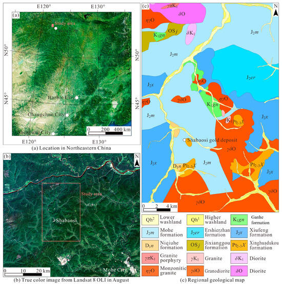
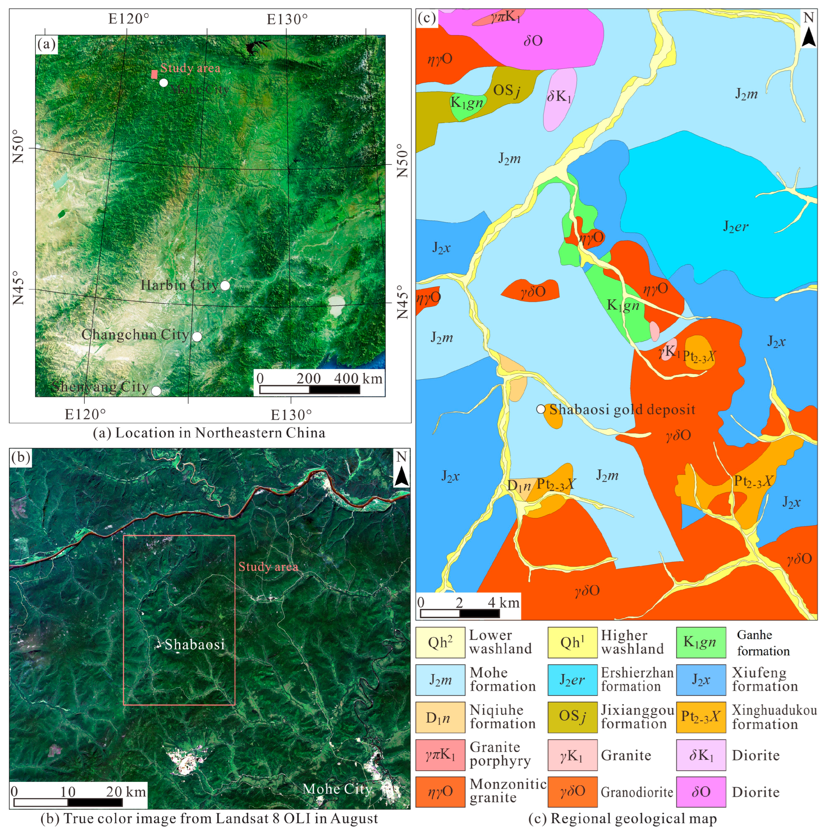
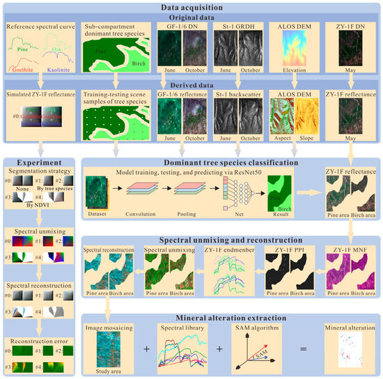
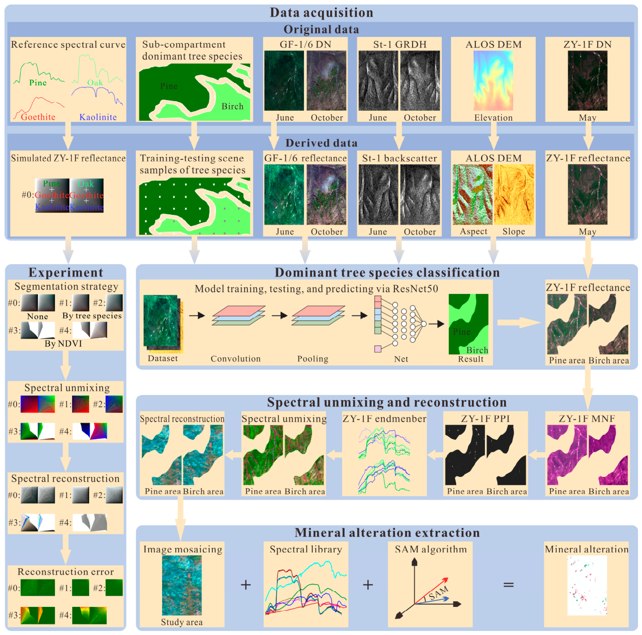
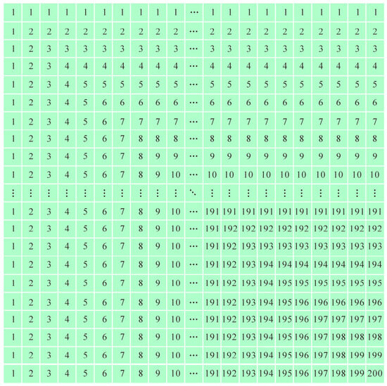
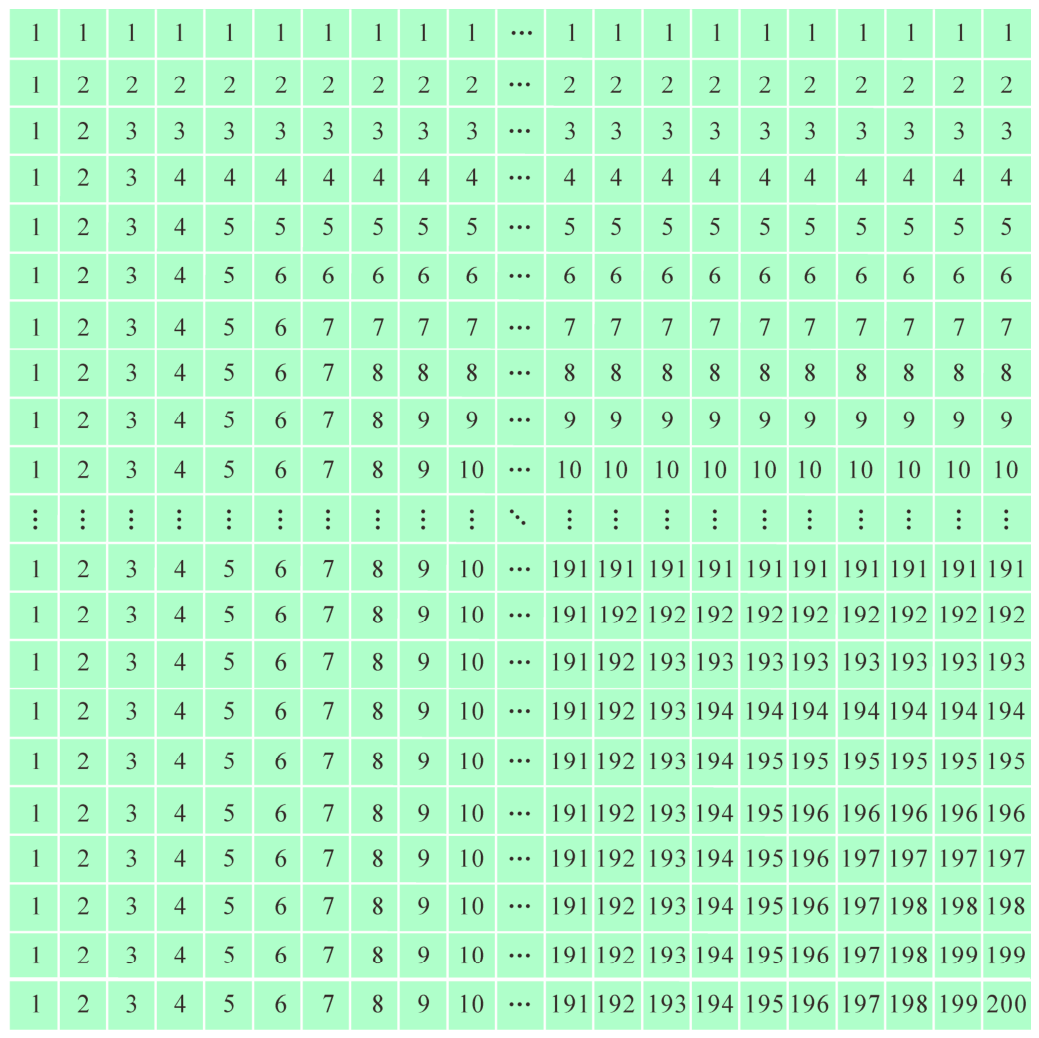
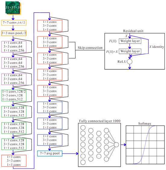
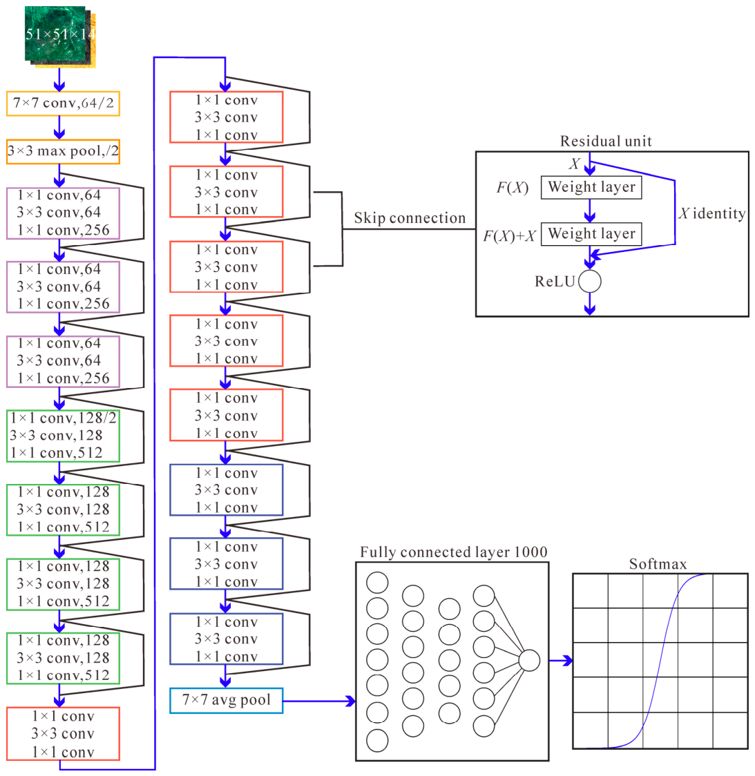
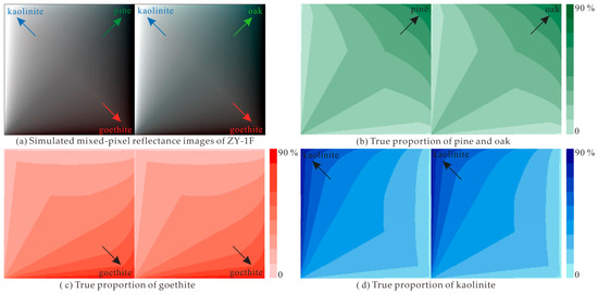
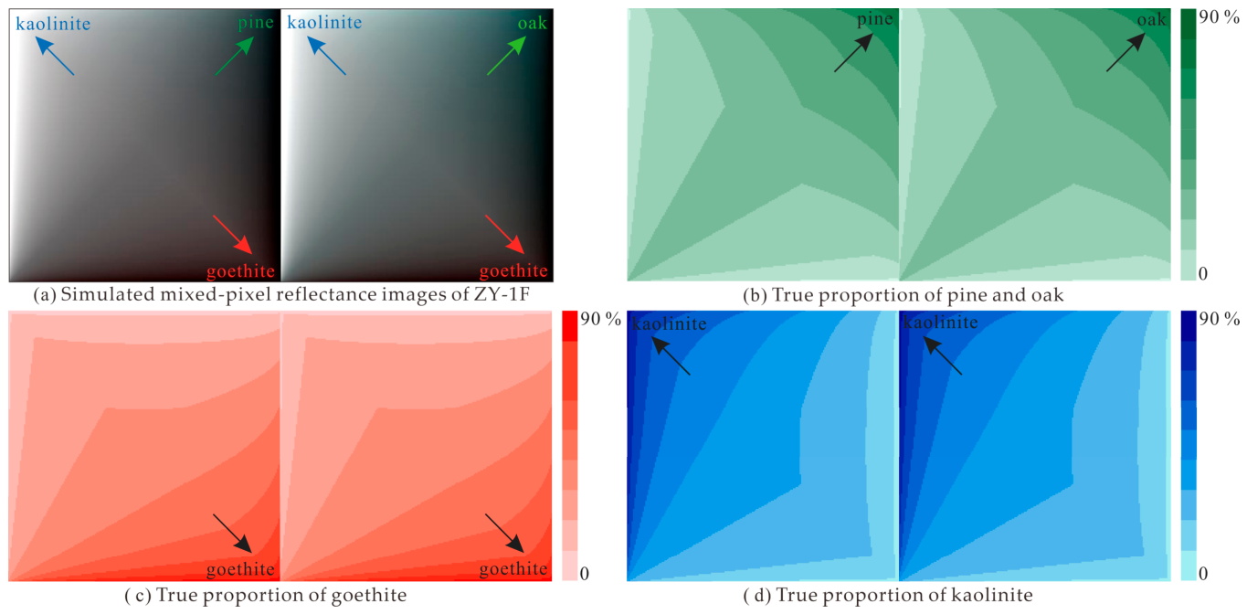
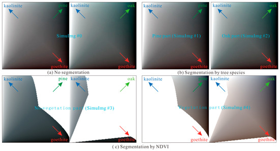
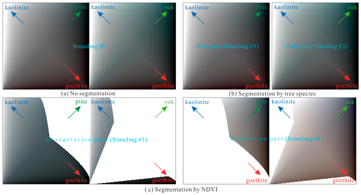
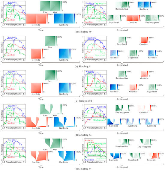
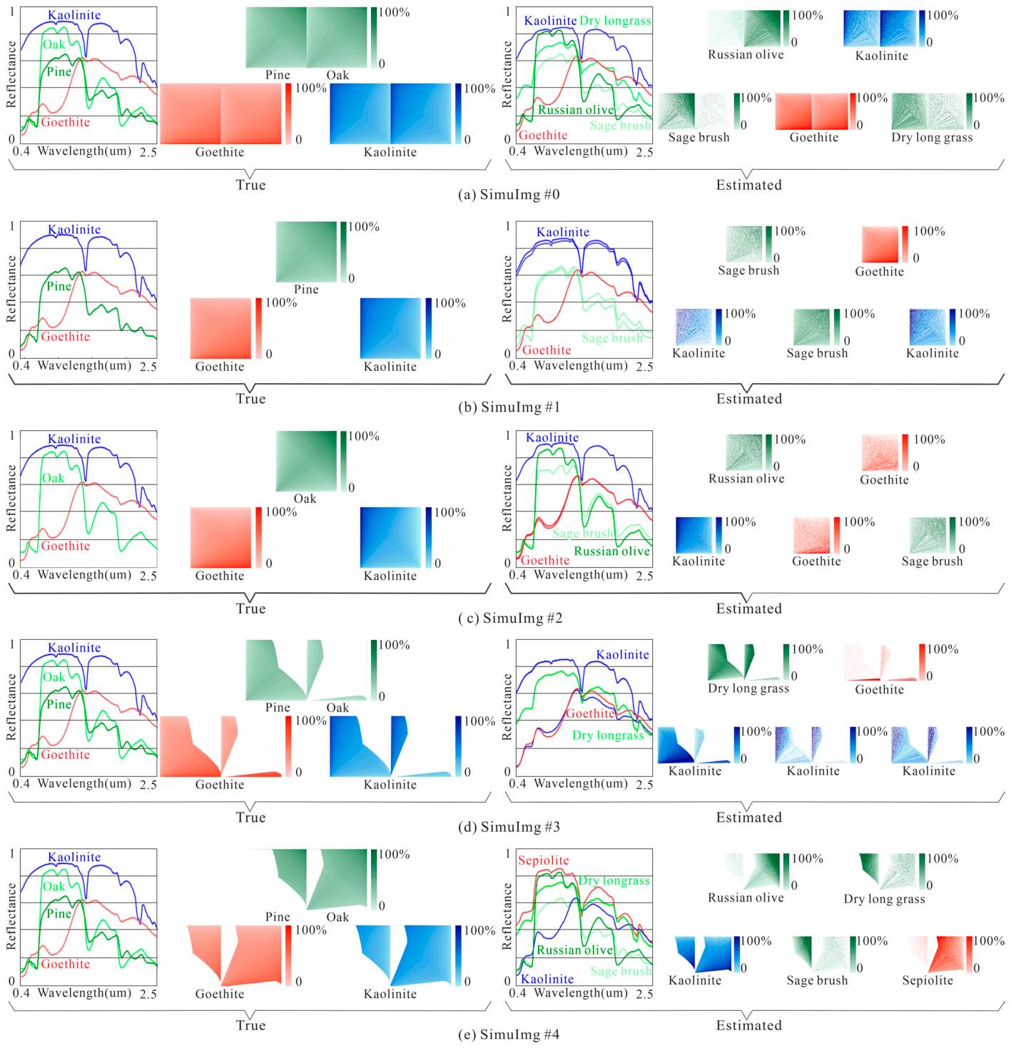
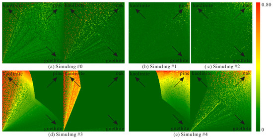
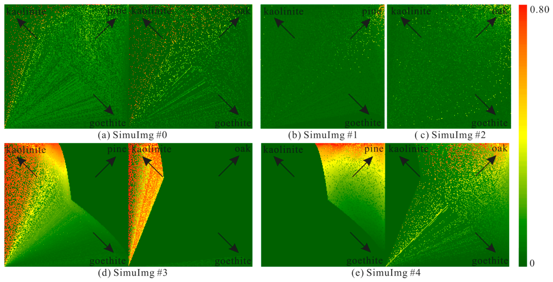
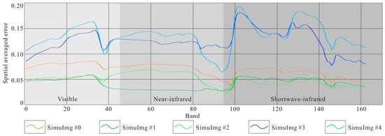
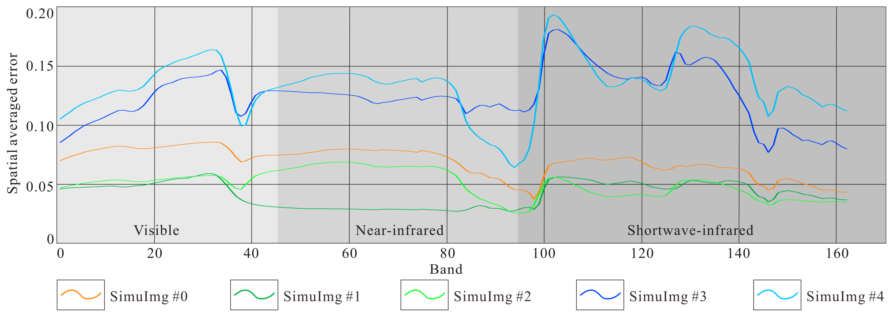
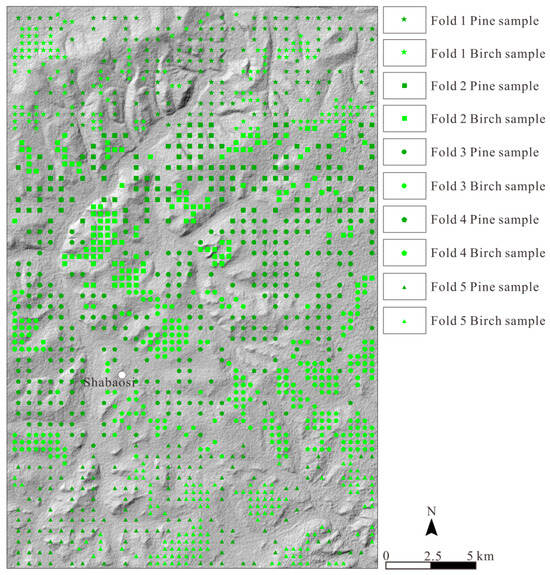
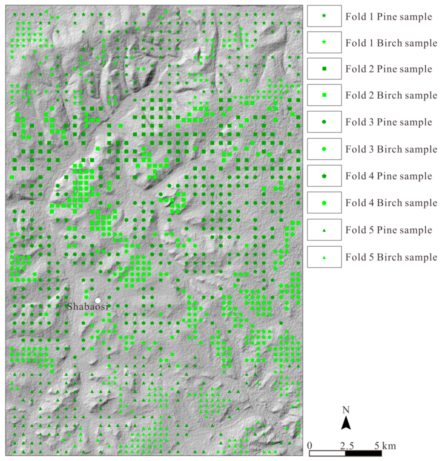
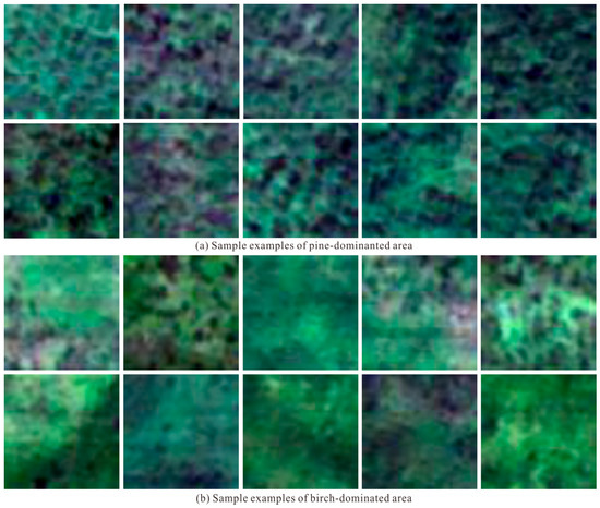
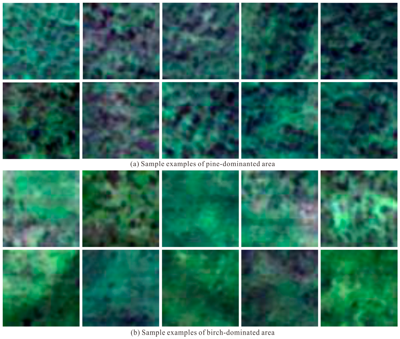
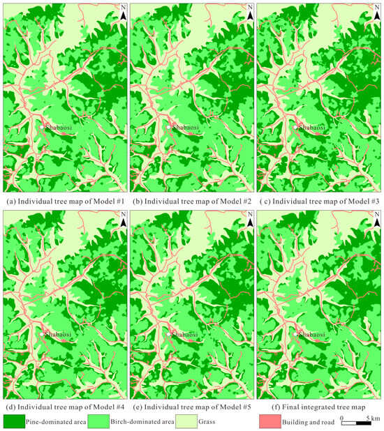
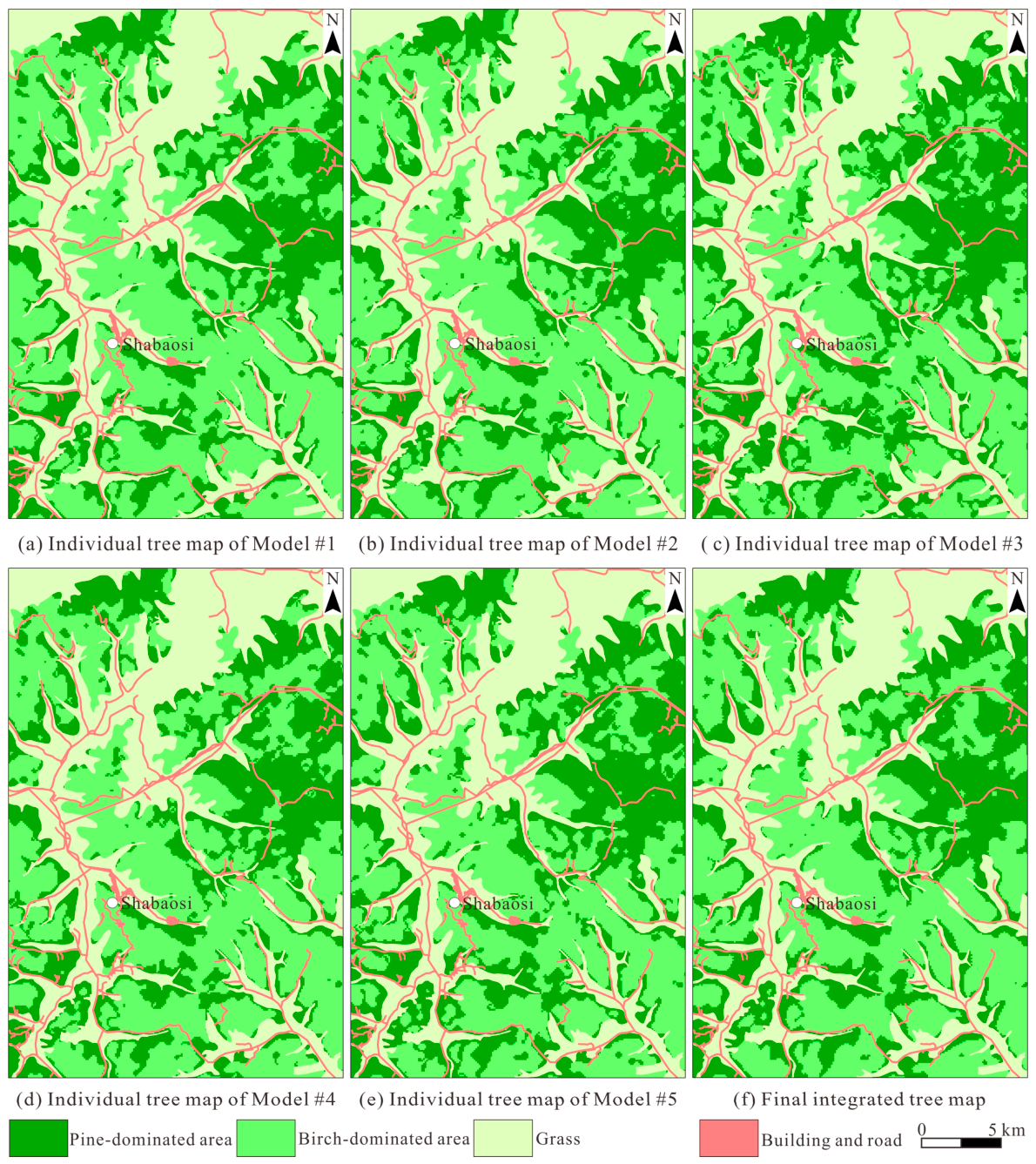
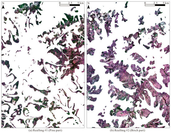
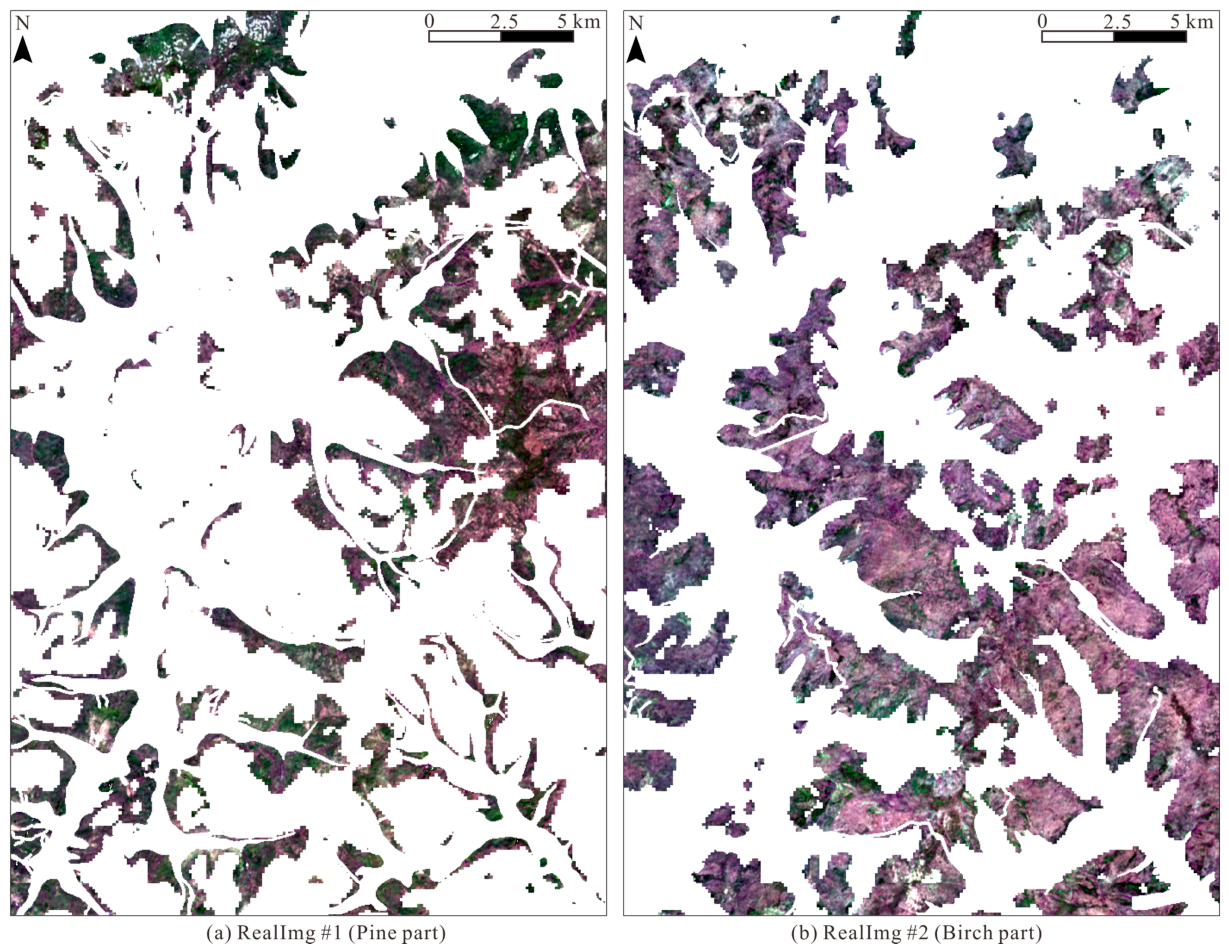
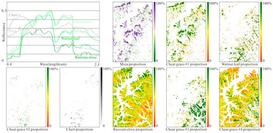
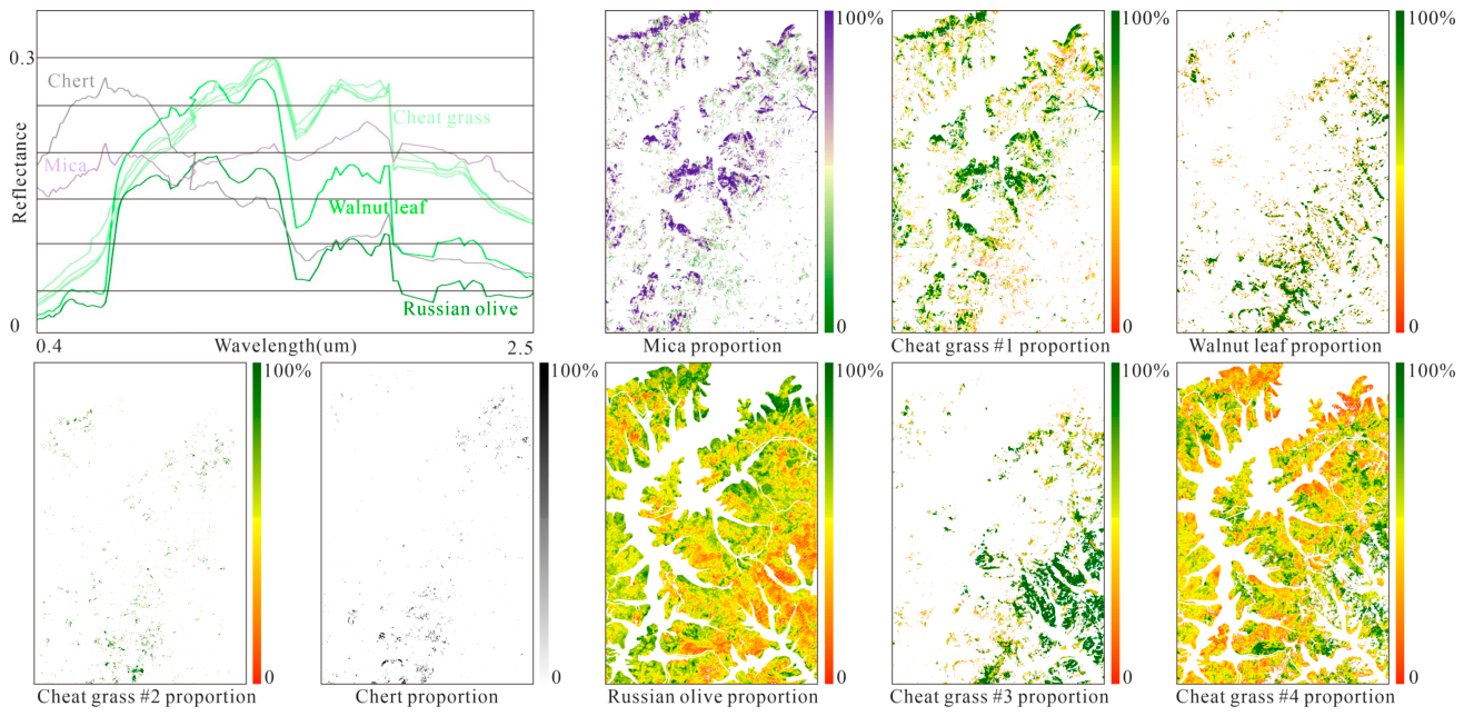
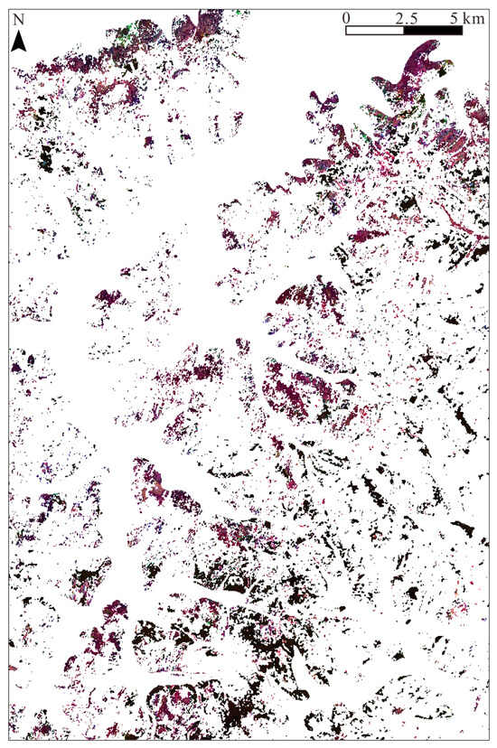
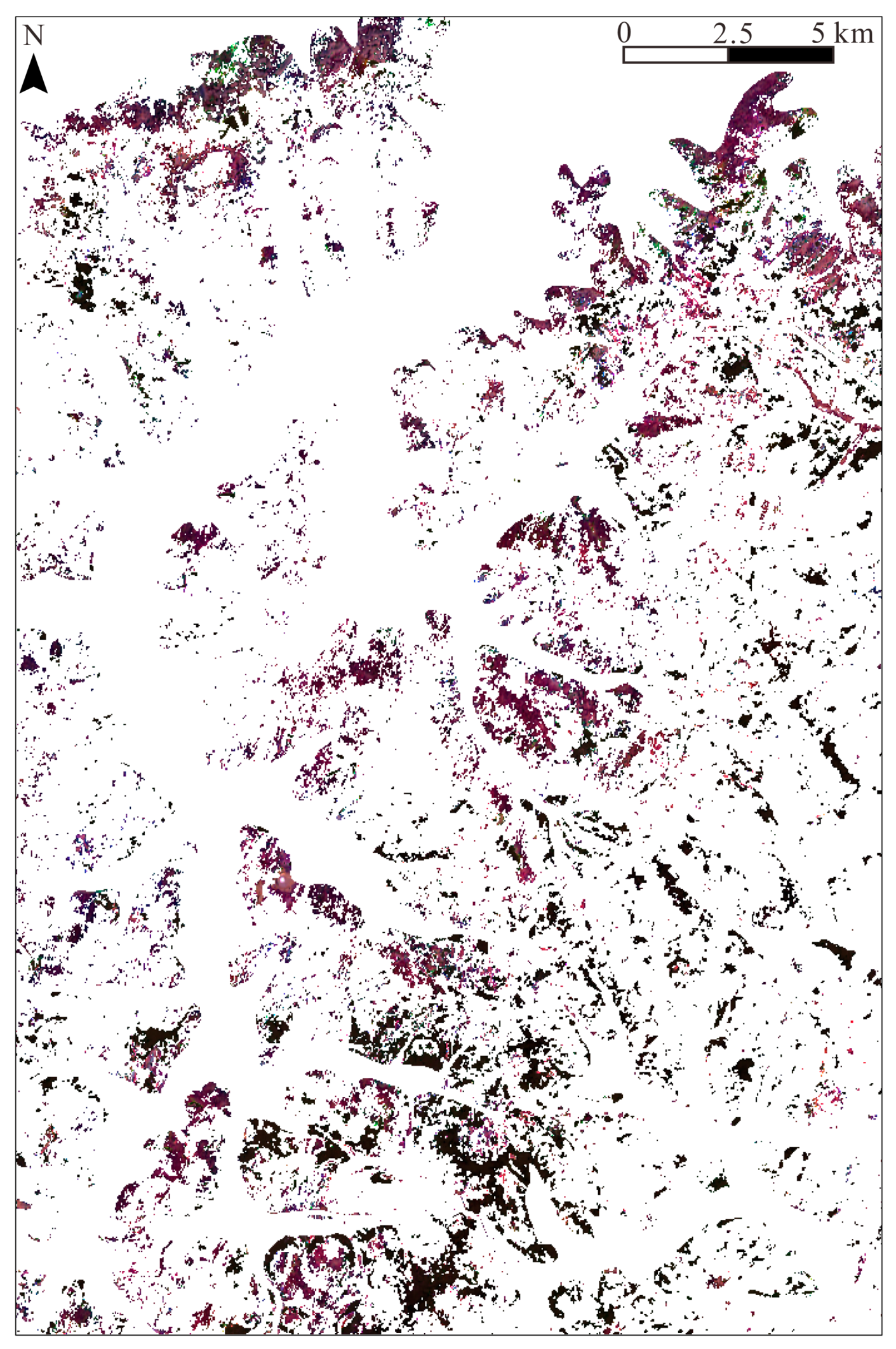
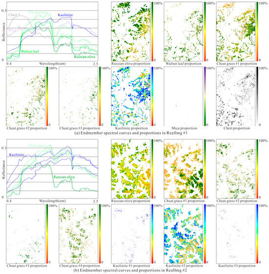
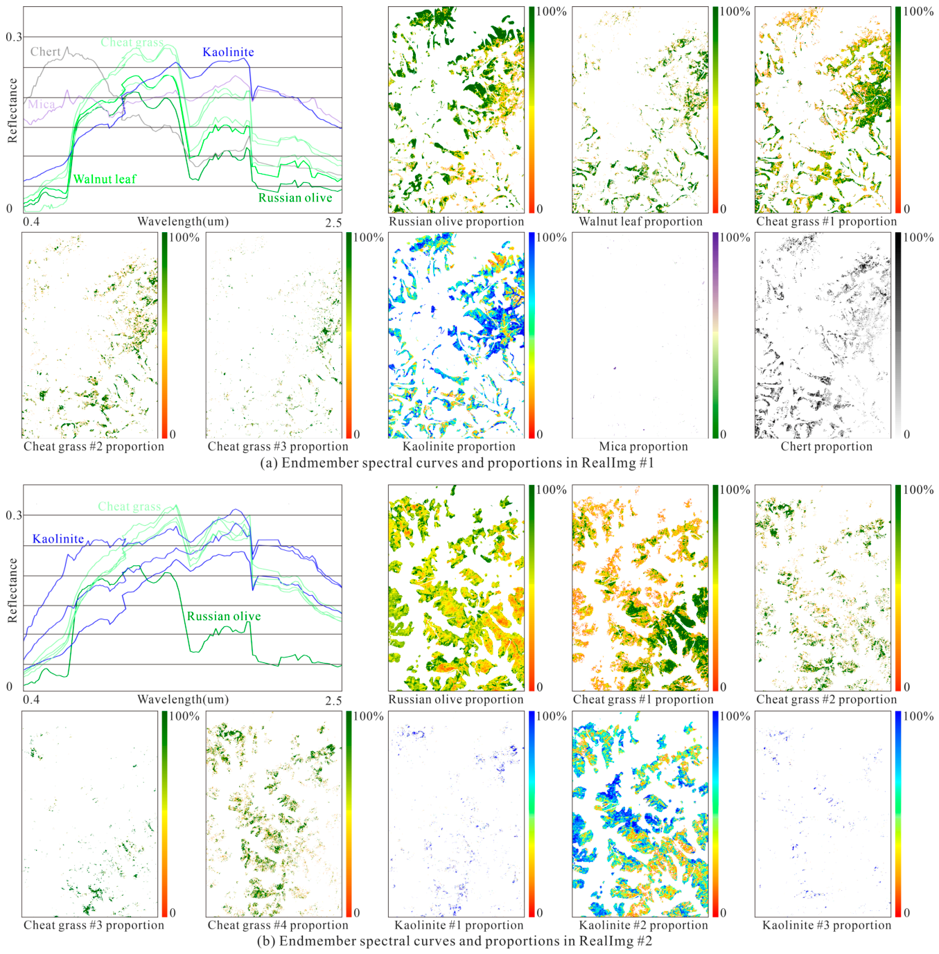
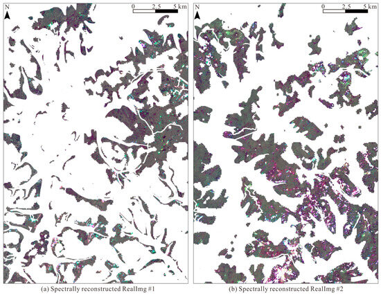
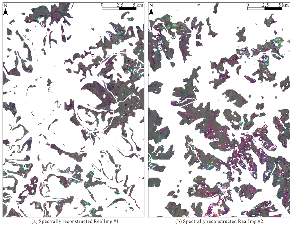
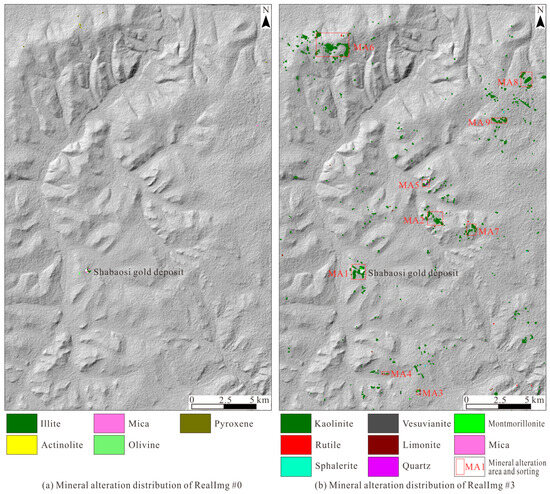
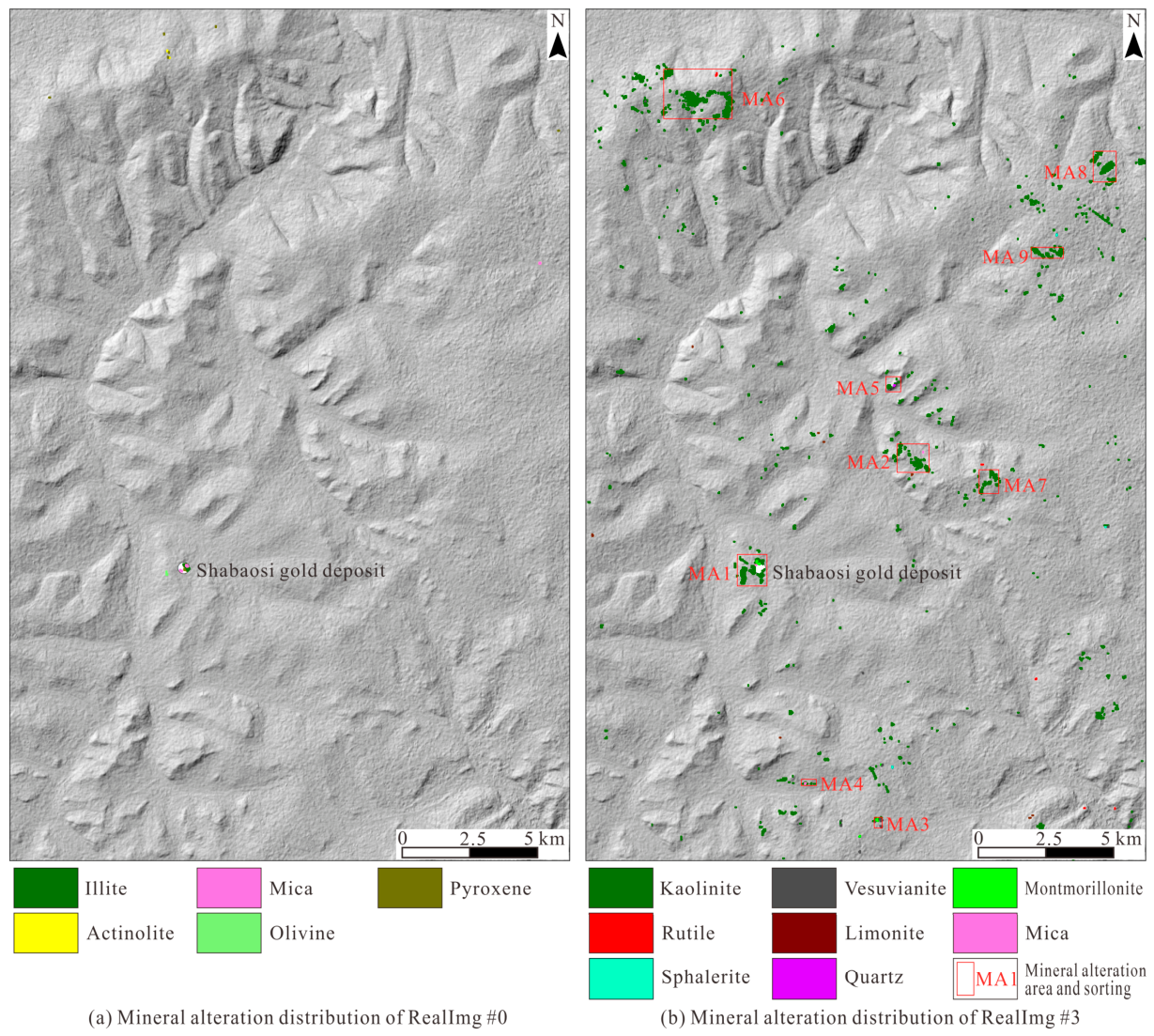
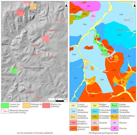
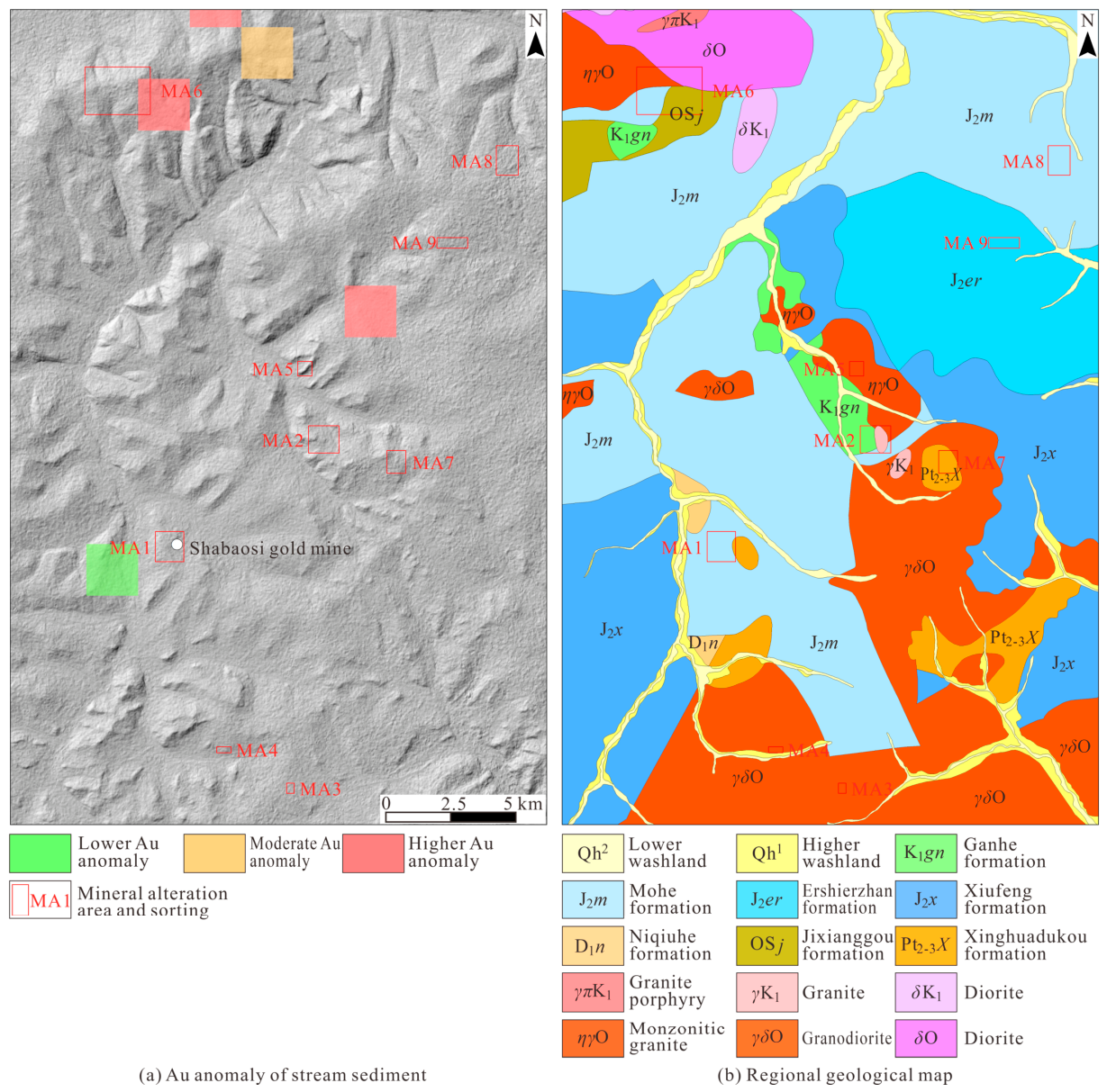
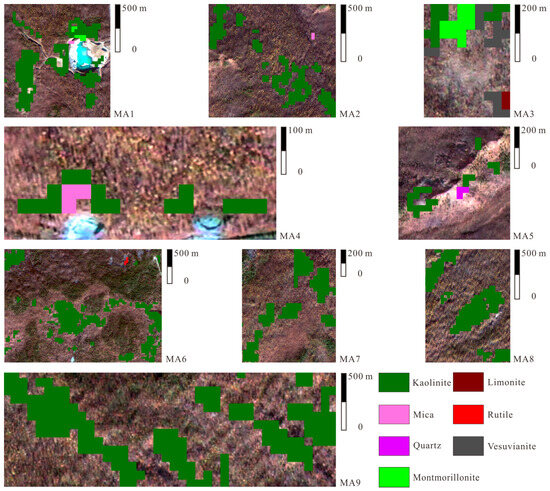
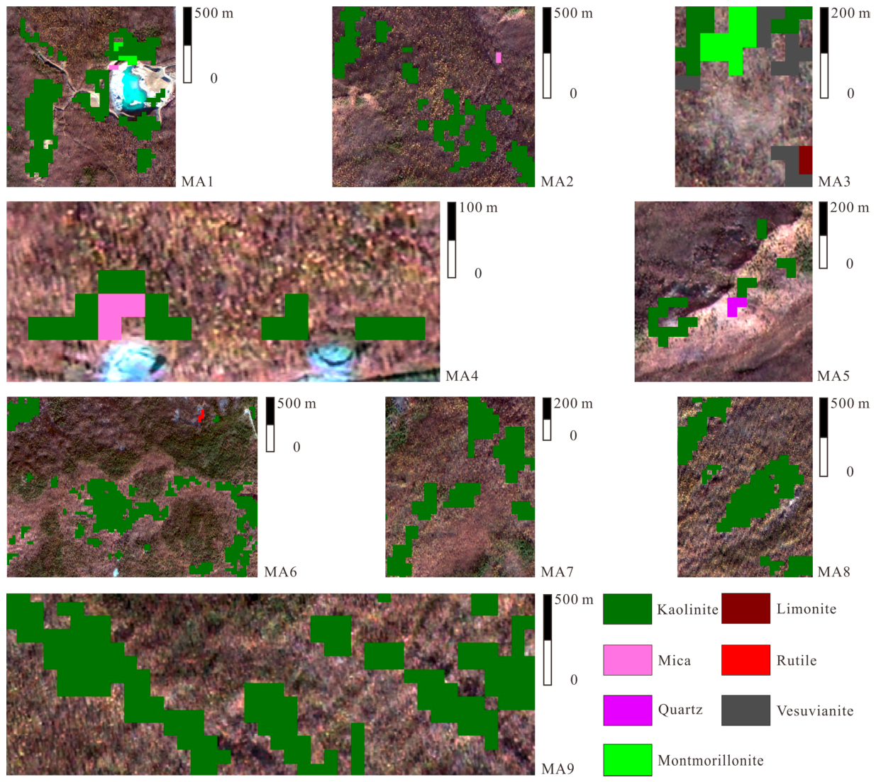

Disclaimer/Publisher’s Note: The statements, opinions and data contained in all publications are solely those of the individual author(s) and contributor(s) and not of MDPI and/or the editor(s). MDPI and/or the editor(s) disclaim responsibility for any injury to people or property resulting from any ideas, methods, instructions or products referred to in the content. |
© 2026 by the authors. Licensee MDPI, Basel, Switzerland. This article is an open access article distributed under the terms and conditions of the Creative Commons Attribution (CC BY) license.