Optimizing Drilling in Brownfield Ni-Cu Depositional Systems Based on the Integration of Geochemical, Geophysical and Drill-Hole Data

Abstract

Effective drillhole placement is critical to the success of mineral exploration, particularly in brownfield settings where subsurface information remains sparse despite the availability of data from adjacent, previously explored areas. To address the challenges of uncertainty in resource estimation and the high cost of drilling, we present a drilling sequence optimization framework guided by geophysical and surface geochemical data. The framework integrates statistical learning and geostatistical simulation to construct a set of prior models of intrusion and nickel grade distribution. These models are used to quantify the expected reduction in uncertainty for each potential drillhole by evaluating their corresponding Efficacy of Information (EOI). This approach allows the sequential selection of drillhole locations that maximize information gain while managing exploration risk. We apply the methodology to a case study in the Curaçá Valley, Brazil, where prior data from a well-characterized nearby zone inform predictions in the adjacent target area. The results demonstrate that incorporating prior geological knowledge from nearby areas into the drilling strategy can significantly improve targeting efficiency and reduce uncertainty in early-stage brownfield exploration.

1. Introduction

The identification of a promising mineral deposit marks only the initial stage of the mineral exploration process. Once geophysical surveys and geochemical soil analyses indicate a potential target, a critical question arises: where should the first drillholes be placed? Drilling operations are expensive and inherently high-risk, highlighting the need for strategies that can guide drilling decisions and reduce uncertainty in resource estimation.

To address these challenges, we develop a drilling sequence optimization framework informed by surface geochemical data, aimed at reducing uncertainty in key deposit parameters, such as ore grade, tonnage, and volume, while managing exploration costs. The framework is applied in a brownfield exploration setting, where prior drilling in neighboring target areas provides a foundation for geological learning. The drilling strategy is formulated as a decision-making process under geological uncertainty, in which each drillhole is selected to maximize expected information gain in a Bayesian sense. This approach requires a set of plausible resource models that reflect prior geological uncertainty as input.

In brownfield exploration, uncertainty in mineral resource estimation remains a critical challenge, despite the availability of some prior drilling data from adjacent or previously explored areas. While data availability is typically greater than in greenfield settings, subsurface information in the target area is often still sparse or unevenly distributed. This, combined with the inherent geological complexity of mineral systems, can lead to significant uncertainty in estimates of ore grade, tonnage, and volume. Such uncertainty poses substantial financial risks, potentially leading to over- or underestimation of ore grade or volume and ultimately affecting project feasibility and planning [1,2]. Accurate and robust mineral resource models are therefore essential for effective risk management and economic evaluation in brownfield contexts [3].

Various methodological approaches have been developed to model and quantify uncertainty. A review of these approaches is provided in [1]. Traditional geostatistical methods, such as kriging, remain widely adopted for resource estimation [3,4]. In parallel, geostatistical simulation techniques [5,6], and more recently, machine learning (ML) approaches [7,8] have gained popularity, particularly for integrating complex, multivariate, and nonlinear datasets to generate spatially coherent realizations of geological structures and grade distributions.

In addition to these methods, quantitative drillhole site selection and optimization strategies have been proposed. Simulation-based and geostatistical approaches aim to identify drill locations that maximize information gain or reduce estimation uncertainty [9,10]. Bayesian optimization methods explicitly define objective functions for additional drillhole placement, enabling systematic trade-offs between exploration cost and information gain [11]. Heuristic and algorithmic methods, including particle swarm optimization and multi-objective selection frameworks, have also been applied to select additional boreholes that improve resource classification and minimize variance [12,13]. These approaches provide a methodological foundation for systematically ranking candidate drillholes, complementing our proposed Efficacy of Information (EOI) framework.

Another valuable strategy in early-stage exploration is the use of data from geologically comparable or adjacent regions that have been previously investigated. These areas often include drillhole assays, geophysical inversion models, and soil and chip geochemical profiles, which can inform modeling efforts in underexplored zones. Prior models of intrusion geometry and structural controls can be effectively used to rank new drill targets in magmatic Ni–Cu systems. For example, magnetotelluric imaging has identified previously unknown anomalies resembling known ore bodies [14], and global analyses show that major discoveries are often controlled by multi-scale structural intersections [15], providing evidence that such prior models can improve drillhole ranking in brownfield exploration. Building on these observations, our framework incorporates prior intrusion and structural knowledge to inform the ranking of candidate drillholes.

In this study, we explore how such prior knowledge can be transferred to generate prior models of intrusion geometry and economic Ni grade distribution that integrate surface geophysical and geochemical data. The challenge is to consider each source of information at its proper scale (volume) and resolution (spacing). In previous work [16], we have shown that, ignoring scale and resolution, simply upscaling all data to the same scale results in overly optimistic predictions. Lithogeochemical constraints provide an additional and complementary source of prior information for intrusion-hosted magmatic Ni–Cu systems, informing both intrusion geometry and grade distribution [17].

The proposed methodology builds on these foundations by combining geostatistical simulation and Bayesian reasoning to construct a set of plausible prior realizations representing both intrusion and grade uncertainty. These realizations are then used to evaluate the Efficacy of Information (EOI) metric [16], which quantifies the expected reduction in uncertainty for each candidate drillhole. EOI provides a computationally efficient alternative to inversion-based approaches, enabling flexible and interpretable ranking of drilling options without requiring full posterior sampling. The framework is applied to a real-world case study in the Curaçá Valley, Brazil, where prior knowledge from a well-characterized anomaly (A1) informs drilling decisions in an adjacent target area (A3).

2. Case Study

The dataset originates from Brazil’s Curaçá Valley, which spans approximately 1700 km² and ranks among the largest copper districts in South America. The valley hosts significant copper and nickel mineralization, primarily associated with mafic–ultramafic intrusions. These intrusions contain economically important copper sulfide deposits. The regional geology is complex, with magmatic deposits of diverse styles of mineralization. Nickel, copper, and cobalt soil geochemical anomalies delineate a continuous trend approximately 15 km in length, associated with underlying mafic and ultramafic lithologies. The scale and continuity of these anomalies suggest the presence of a potentially significant Ni-Cu mineral system, with potential for high-grade sulfide mineralization [18].

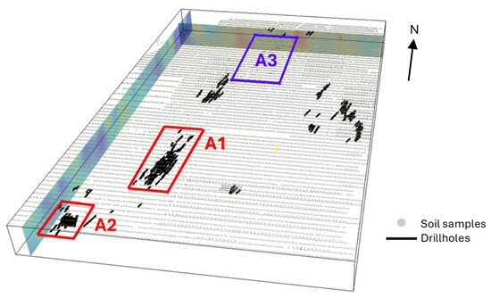
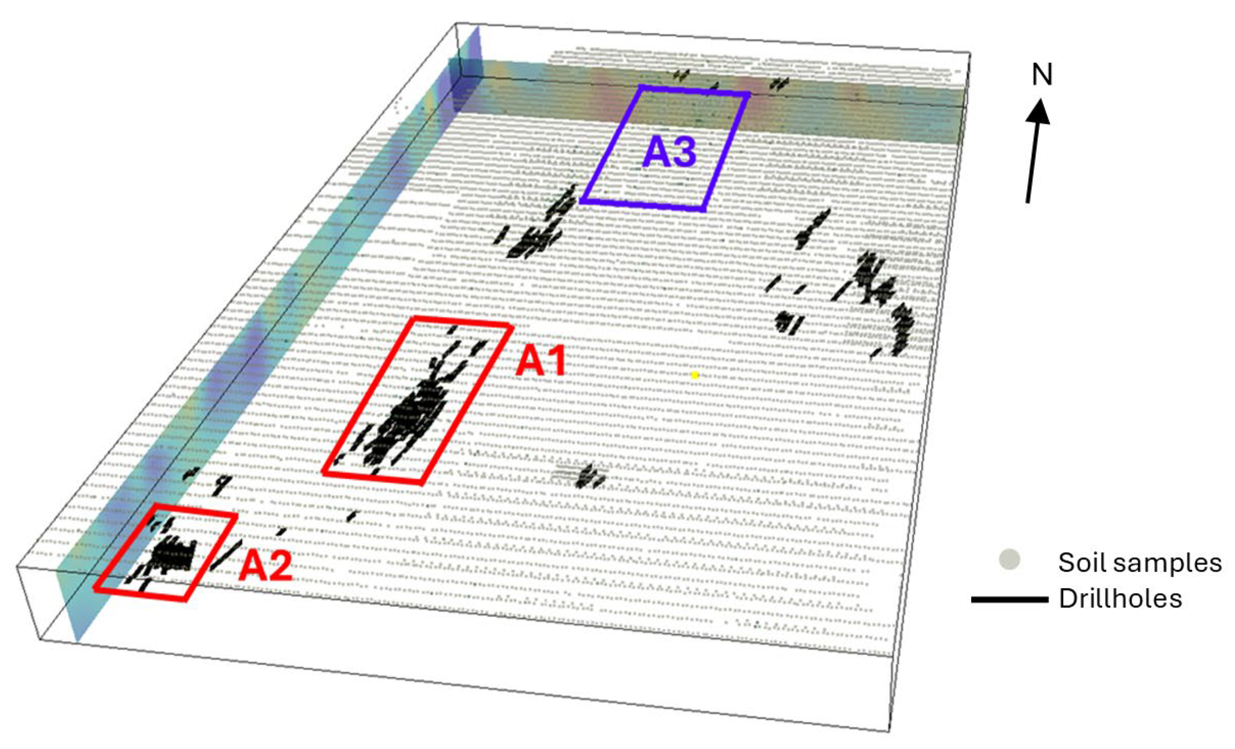
Several areas within the valley, notably Anomaly 1 (A1) and Anomaly 2 (A2), have been extensively explored and have led to the discovery of mineral inventory. Extensive drilling campaigns, geophysical and geochemical soil data are available for A1 and A2 and were used to better characterize the shape, volume, and grade of the intrusion. The locations of the 3 anomalies are shown in Figure 1.

Figure 1. Area under investigation, highlighting the 3 anomalies of interest, geochemical soil samples (gray dots), and drillhole campaign (black lines).

Within that trend, geologists have identified a new target area, Anomaly 3 (A3), situated along the structural continuation of A1 and A2, where mineralization is also expected.

The objective of this study is to define an optimal drilling strategy for A3 with the aim of reducing uncertainty in grade and tonnage estimates derived initially from geochemical and geophysical data only. To achieve this, we employ the EOI framework described below with a particular focus on the construction of the prior model using information from nearby areas.

3. Review of Methods

3.1. Efficacy of Information

Efficacy of information (EOI) has been proposed by Caers et al. [16] to define an optimal drilling sequence in mineral exploration. The main idea behind EOI is to quantify, on average, how much information on some property of interest θ (also named reward) is provided when acquiring new data. This can be quantified by evaluating how much the posterior distribution of the reward f(θ|d) differs from the prior distribution f(θ) when acquiring some data d and can be expressed by KL divergence between the prior and the posterior distribution of the reward θ:

$$D_{KL}\left(f(\mathit{\theta }|d)\parallel f\left(\mathit{\theta }\right)\right)=-{{\displaystyle \int }}_{\mathit{\theta }}f(\mathit{\theta }|d)log\left({\displaystyle \frac{f\left(\mathit{\theta }\right)}{f(\mathit{\theta }|d)}}\right)d\mathit{\theta }$$

(1)

Because the new data d is not known (future), EOI integrates this difference over all possible d, as obtained by the prior distribution of the models:

$$EOI\left(\mathit{\theta }\right)=-{{\displaystyle \int }}_d{{\displaystyle \int }}_{\mathit{\theta }}f(\mathit{\theta }|d) f\left(d\right) log\left({\displaystyle \frac{f\left(\mathit{\theta }\right)}{f(\mathit{\theta }|d)}}\right)d\mathit{\theta }dd$$

(2)

To practically evaluate EOI, a Monte Carlo simulation approach is used, whereby a set of L prior models $m^{\left(\mathcal{l}\right)}, \mathcal{l}=1,\dots ,L$ of the subsurface is generated and the associated rewards ${\mathit{\theta }}^{\left(\mathcal{l}\right)}$ and data $d^{\left(\mathcal{l}\right)}$ are computed from the prior models. In most cases, $d$ is high-dimensional, hence dimensionality reduction is applied to obtain low-dimensional data, denoted $d^{\ast \left(\mathcal{l}\right)} .$ EOI is then expressed as follows:

$$\mathrm{EOI}\left(\mathit{\theta }\right)={\displaystyle \frac{1}{L}}{\displaystyle \sum }_{\mathcal{l}=1}^L{D}_{KL}\left(f(\mathit{\theta }|d^{\ast \left(\mathcal{l}\right)} \left|\right| f\left(\mathit{\theta }\right) \right)$$

(3)

The data configuration (or survey geometry) that maximizes the EOI is the optimal choice.

The EOI outcome depends largely on the definition of the prior model and the reward function, as well as the chosen data configuration (e.g., the locations of drillholes). Unsurprisingly, different optimal drilling paths may be obtained for different rewards (e.g., volume, maximum grade, etc.). Additionally, a poorly chosen prior model may result in a non-optimal drilling sequence. As a practical guideline, the EOI procedure typically requires a few hundred prior models to achieve robust results, given that only a scalar (grade or tonnage) is being estimated.

3.2. P-Field Simulation

Our approach involves the 3D geostatistical simulation of intrusion vs non-intrusion constrained to soft data (geophysics) and hard data (drillholes). A method that works well in this context is p-field simulation, which requires a 3D probability model of the intrusion indicator and a variogram for the intrusion model as input. Introduced by Srivastava in 1992, Probability Field (P-field) Simulation is a geostatistical technique designed to integrate uncertainty from soft data (through local probability distributions) into spatial modeling [19]. The approach involves generating spatially correlated fields of uniformly distributed random numbers (p-field), which are then used with the local conditional cumulative distribution functions (CCDFs) to assign values at each grid location. This process enables the generation of multiple equally probable realizations that capture spatial variability consistent with the input data. We will use this approach in the generation of geostatistical models, which is needed to calculate the above EOI.

The p-field simulation algorithm comprises three fundamental steps:

• Local uncertainty modeling: At each unsampled location, a CCDF is estimated to quantify the uncertainty of the target variable. This CCDF reflects the probability distribution of potential values at that location, conditioned on surrounding data. Techniques such as indicator kriging are commonly used to construct these CCDFs.
• Probability field generation: A spatially correlated random field of probability values, referred to as the p-field, is simulated unconditionally. This field is characterized by a uniform marginal distribution and a spatial covariance structure that mirrors the spatial correlation of the target variable. Sequential Gaussian Simulation is used in this paper [20].
• Value sampling: For each grid node, the simulated value of the target variable is obtained by sampling from the corresponding CCDF using the p-field value at that location as the quantile level.

This procedure enables the generation of multiple, equally probable realizations that preserve both local uncertainty and spatial continuity. P-field simulation is computationally efficient and allows an easy integration of soft data into the simulation, a functionality we will rely on to integrate geochemical and geophysical data.

3.3. Co-Located Sequential Indicator Simulation (Co-SISIM)

Co-SISIM [21] is a geostatistical simulation technique used for modeling discrete variables. It combines Sequential Indicator Simulation (SISIM) with secondary data, typically from a co-located source like probability maps. The method improves spatial realism by conditioning simulations on both primary (e.g., drillhole if available) and co-located secondary information. It is especially useful in complex geological settings with limited hard data.

3.4. Geochemical and Geophysical Geostatistical Learning

In a brownfield approach, when investigating new regions with potential mineralization, geologists analyze nearby, better-characterized areas to infer the underlying geological system. This helps in constructing conceptual models of the orebody in unexplored zones, particularly those lacking direct subsurface data (e.g., drillholes). Similarly, we propose to learn geostatistical relationships by extracting patterns and insights from existing geophysical and geochemical datasets and studying how they relate to mineralization (e.g., grade). Applying the learned geostatistical relationships to target areas generates improved prior models, which can more effectively guide drilling strategies in underexplored areas.

Two geostatistical models can be learned in the early stage of exploration:

• Learning based on geophysical data: Prior models of intrusion are often generated based on geophysical data (magnetic and ground gravity inversion). Higher values are generally associated with an increase in mafic-ultramafic rocks (intrusions). This relationship can help identify geophysical values that increase the chance of intrusion.
• Learning based on geochemical (soil) data: It is expected that soil geochemistry contains information about the minerals present in the subsurface and, consequently, the desired elements on an anomalous or non-anomalous scale.

If a successful relationship is trained in nearby, well-explored areas, it can predict, using the geophysical and soil data in the new area, a set of prior models of the intrusion and grade.

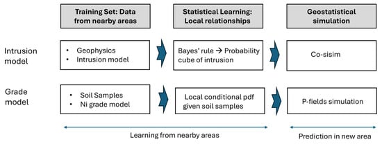
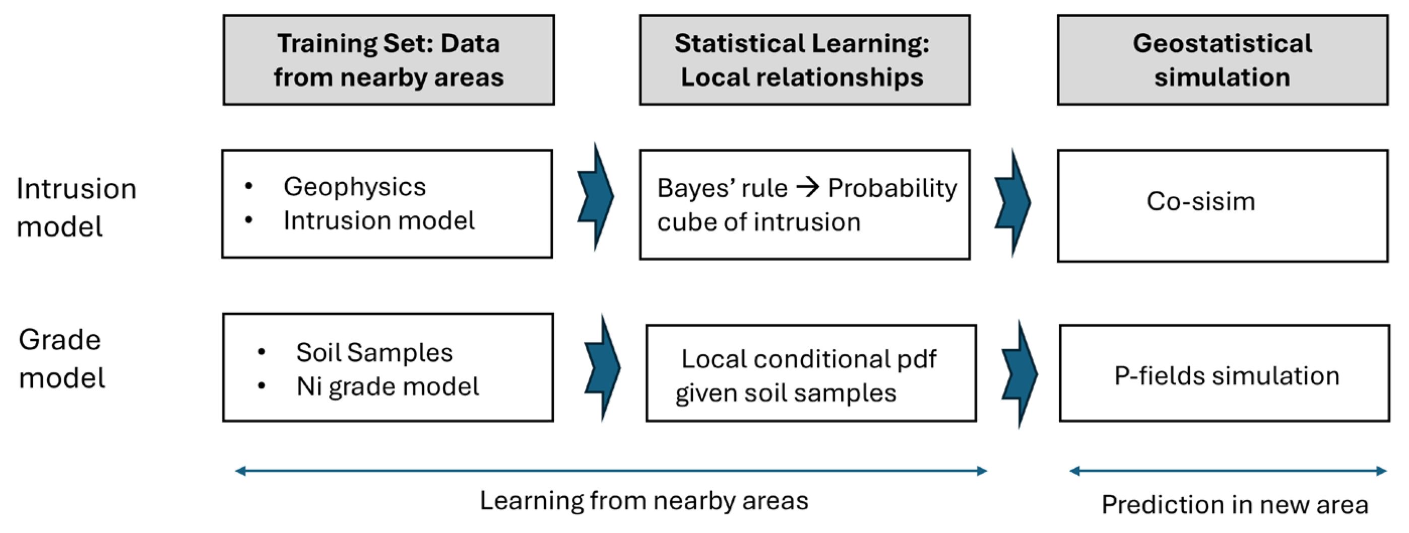
A summary of the approach to generating prior models on intrusion and Ni grade is shown in Figure 2:

Figure 2. Steps proposed to model uncertainty in intrusion and Ni-grade for new areas.

4. Application

Given the spatial proximity of A3 to A1 and A2, we expect geological similarities. Both A1 and A2 have extensive drilling, geochemical, and geophysical datasets, which have been used to develop detailed grade and intrusion models. Across the broader valley, available data includes magnetic and ground gravity inversion results, as well as geochemical soil samples. However, drillhole data are only present in previously explored zones.

4.1. Geochemical and Geophysical Similarity Analysis Between Well-Explored Areas and the New Area

A preliminary step involves identifying which existing datasets and areas are most relevant for informing predictions in the new target area. We adopt the approach described in [22], which analyzes similarity in multivariate data across different locations to rank potential target areas based on their geophysical similarity to existing economic deposits. In this study, we have geophysical data (magnetic and inverted density) and geochemical data from two well-characterized areas, A1 and A2, to assess their potential usefulness in predicting conditions in the less-explored area, A3.

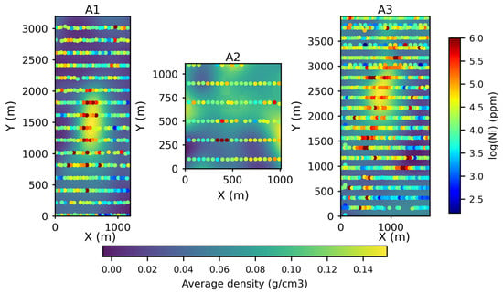
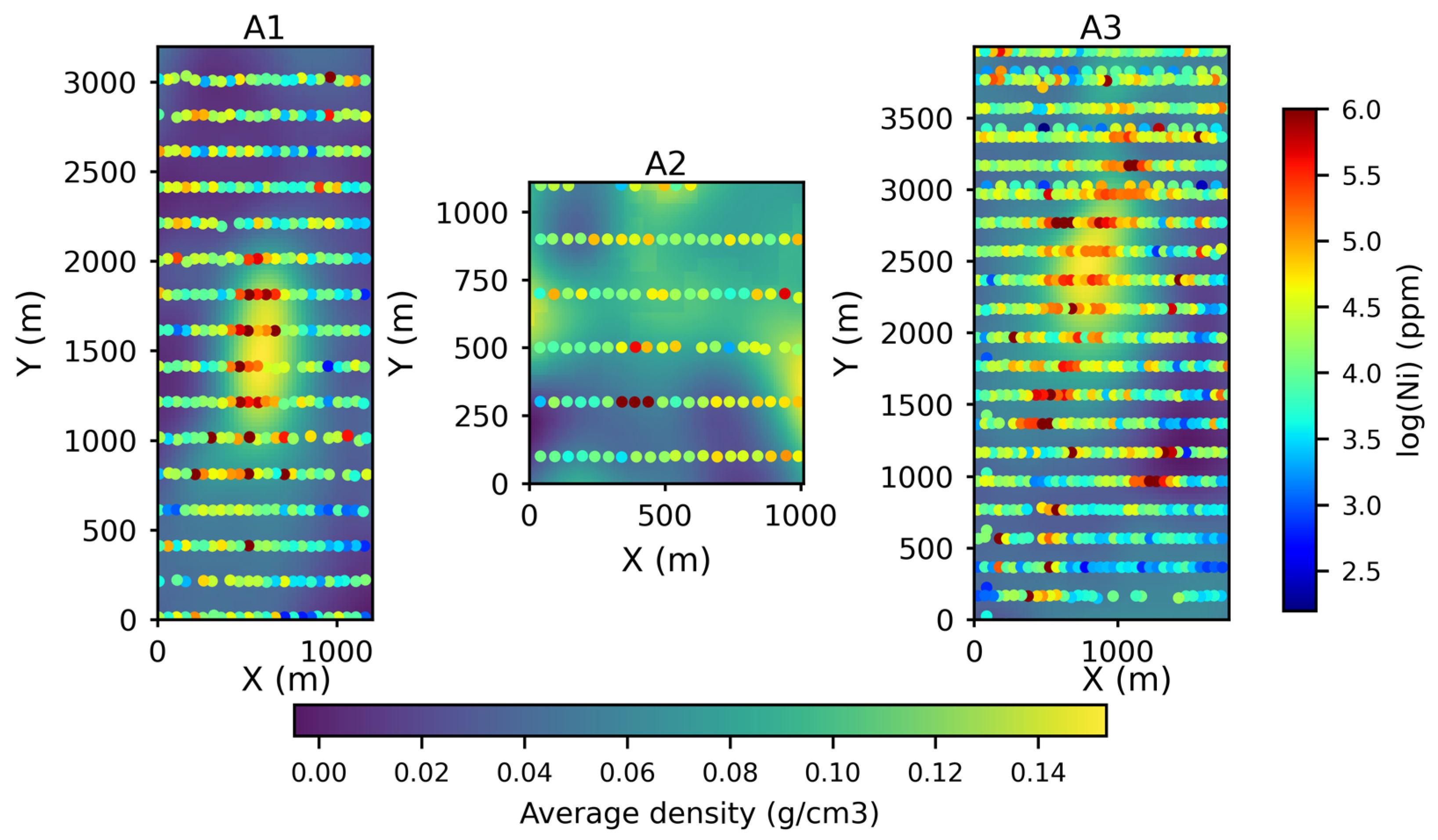
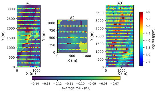
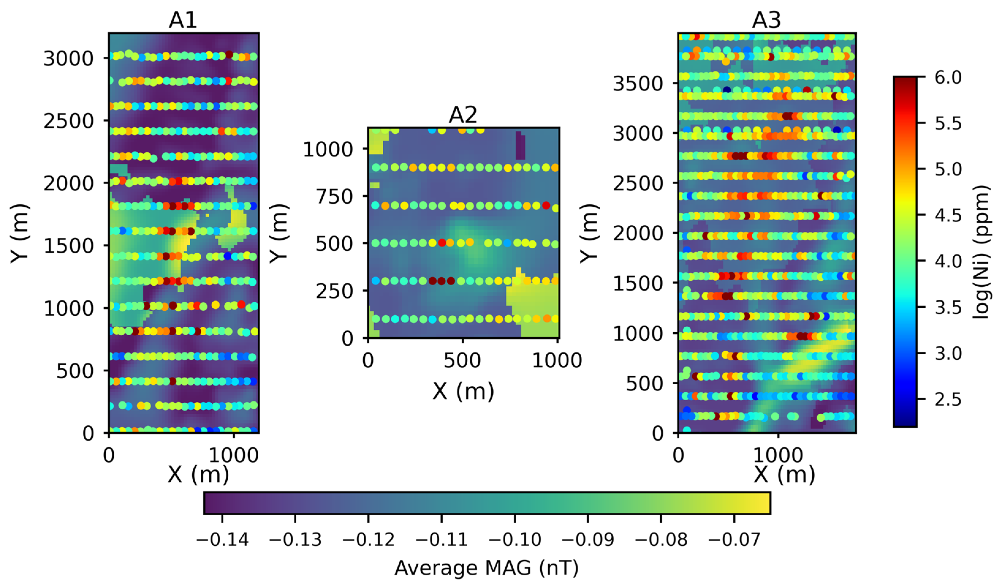
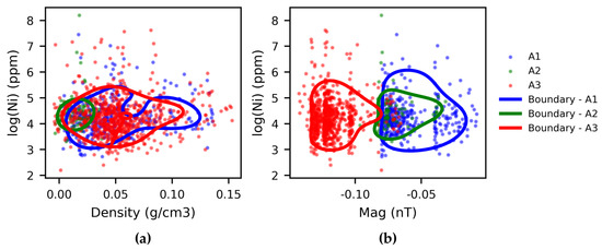
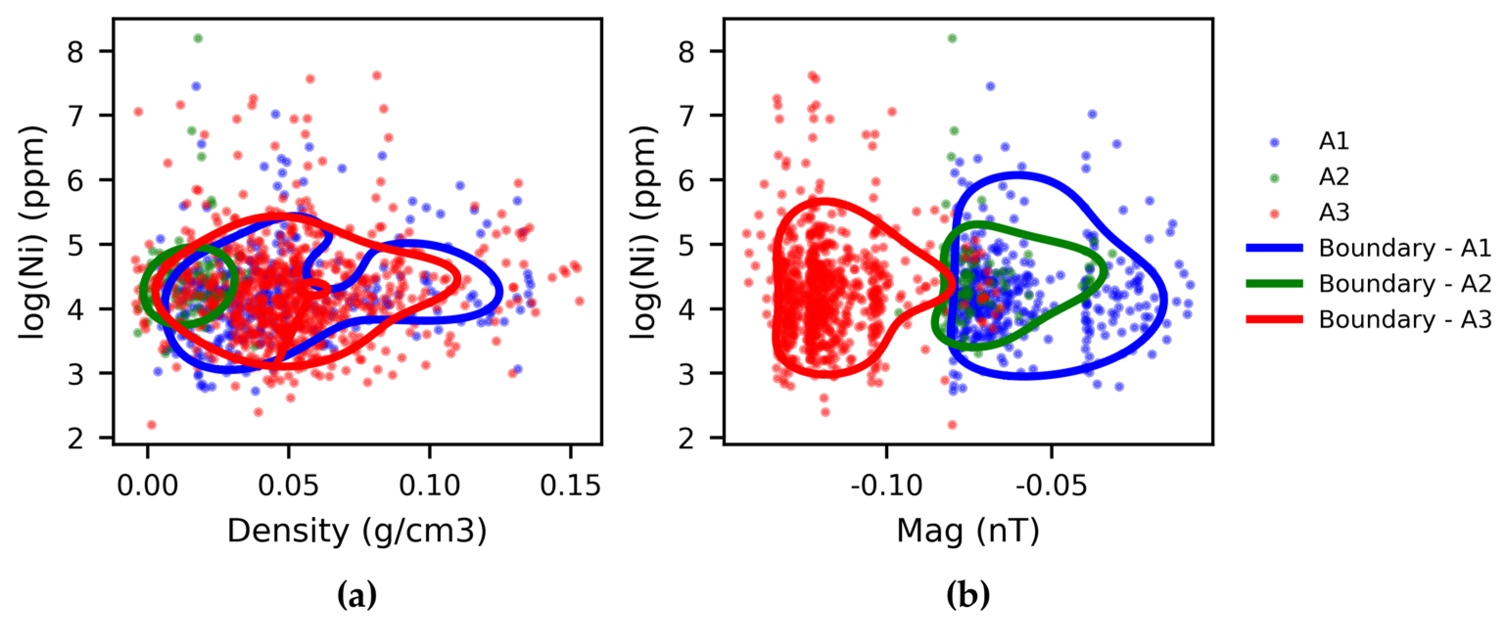
To assess the relationships between geophysical variables and soil geochemistry, magnetic and density values were averaged over depth and extracted at soil sample locations. Maps showing the superposition of depth-averaged geophysical data (density in Figure 3 and magnetic data in Figure 4) with soil samples for all anomalies (A1, A2, and A3) are presented. To further explore the similarities and differences between the anomalies, scatter plots are shown in Figure 5. The left panel displays scatter plots of depth-averaged inverted density versus log-transformed Ni concentrations at soil sample locations for the three areas (A1, A2, and A3), while the right panel presents the corresponding plots for averaged magnetic data. Following the method of [22], we apply a one-class support vector machine (OC-SVM) with a Gaussian kernel to construct boundaries around the main data clusters. These boundaries (or convex hulls) allow for visual and quantitative comparison of the multivariate relationships.

Figure 3. Superposition of depth-averaged density with soil samples for all anomalies (A1, A2, and A3).

Figure 4. Superposition of depth-averaged magnetic data with soil samples for all anomalies (A1, A2, and A3).

Figure 5. Relationship between geophysical and geochemical data for the two well-explored areas A1 and A2 and the target area A3; (a) inverted density; (b) magnetic data.

As Figure 5a, the data from A2 (green) occupies only a narrow subset of the range observed in A3 (red), suggesting that models trained on A2 may involve substantial extrapolation and may not generalize well to A3. In contrast, there is a much stronger overlap between A1 (blue) and A3 (red), indicating that inverted density and log (Ni) concentrations from A1 may be informative for predicting in A3. However, the right panel of Figure 5 shows no overlap in the magnetic data between A1 or A2 and A3, suggesting that magnetic data may not be predictive for A3 in this context.

4.2. Construction of Ni-Grade Model for New Target Area

The prior model is built using a multistage process that includes both the geometry of the intrusion and the distribution of Ni grades. Each part is developed in two steps. First, relationships are learned from training data collected in A1. Then, these relationships are applied to the new area A3, using its available data to generate the corresponding models. Finally, the intrusion geometry and Ni grade models are combined to create the complete prior model.

4.2.1. Geophysical Inversion to Inform Intrusion Geometry

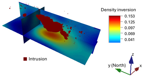
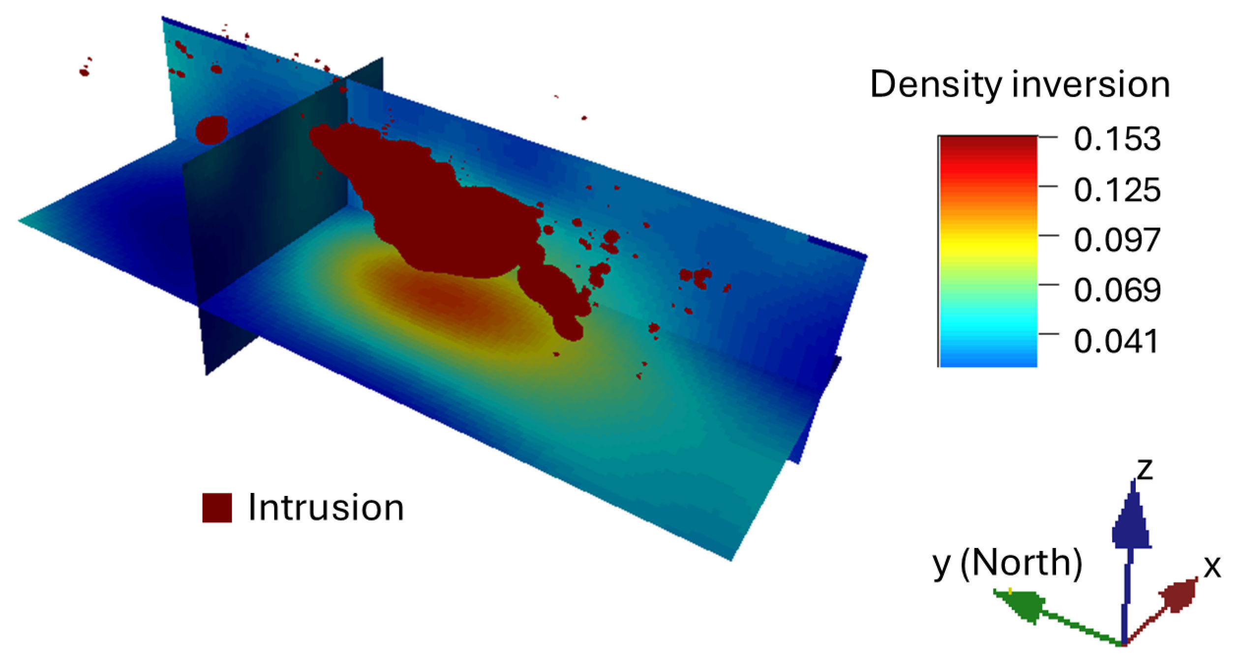
In A1, the inverted density model has shown a strong spatial correlation with the intrusion, as illustrated in Figure 6. The observed overlap between the two models supports the hypothesis that density is a reliable proxy for intrusion in this area.

Figure 6. Intrusion model (red) and 2D slice of the density inversion for A1.

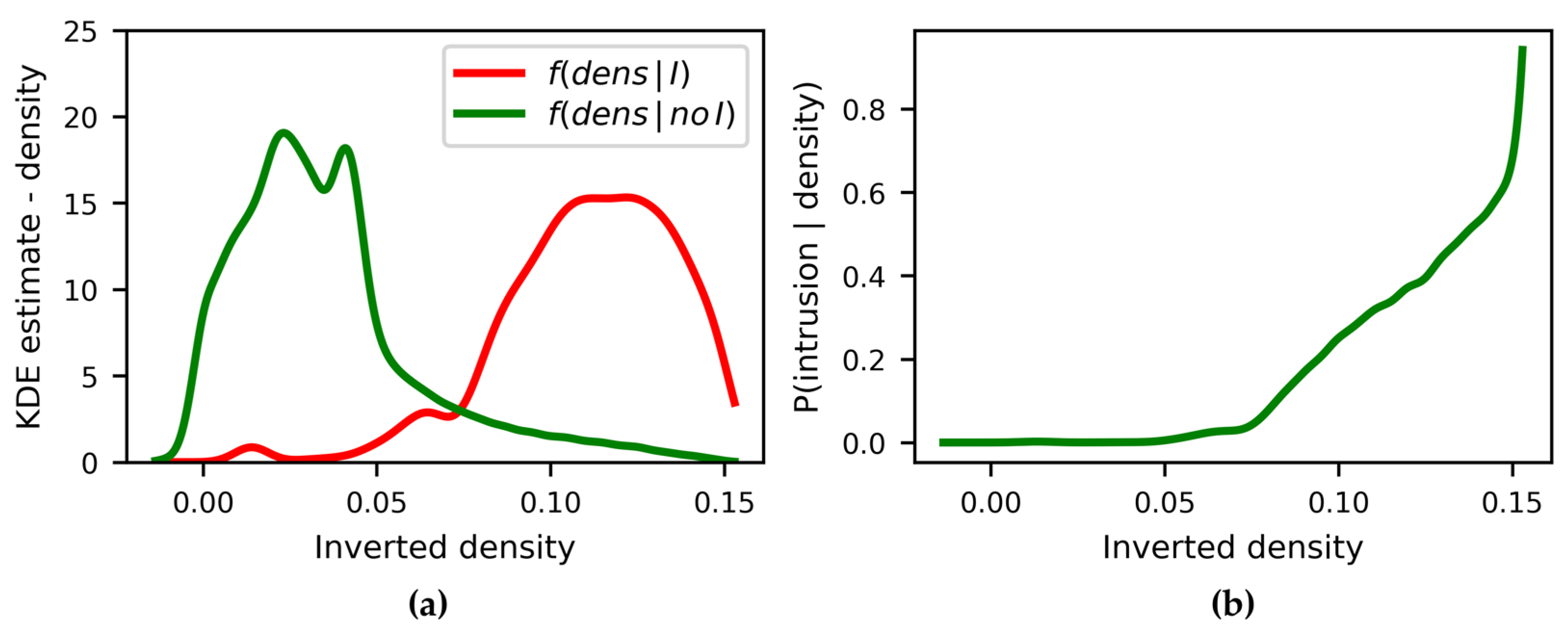
In A3, a density model is available, but an intrusion model has not yet been established. To address this, we learn the relationship between the inverted density model and the corresponding intrusion model for A1. Using this trained model, we aim to infer the probability of intrusion in A3 based on the available density data. This relationship is formalized using Bayes’ rule to estimate the posterior probability of intrusion given density:

$$P(intrusion|density)= {\displaystyle \frac{f(density|intrusion)\ast p_{intrusion}}{f\left(density\right)}}$$

(4)

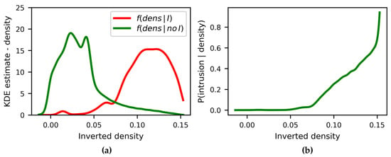
Figure 7a shows a strong correlation between density and intrusion: grid cells identified as part of the intrusion generally present high-density values. By applying Bayes’ rule, we estimate the probability of intrusion conditioned on density values: P(z = 1│density(u)) at location u (Figure 7b). This relationship is then used to generate a probability map of intrusion in A3, based on its observed density data. The resulting probability map serves as input for the generation of prior intrusion models using co-SISIM. A set of 500 models were generated on a 71 × 100 × 105 grid.

Figure 7. (a) Conditional probability density function of the inverted density model given intrusion (I) and non-intrusion (no I); (b) resulting cumulative probability density function.

In the absence of drillhole data in A3, experimental variograms could not be reliably estimated. We therefore use an isotropic spherical variogram with a range uniformly varied between 10 and 30 grid cells, introducing uncertainty while deferring precise modeling until additional drilling data are available.

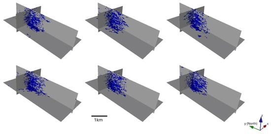
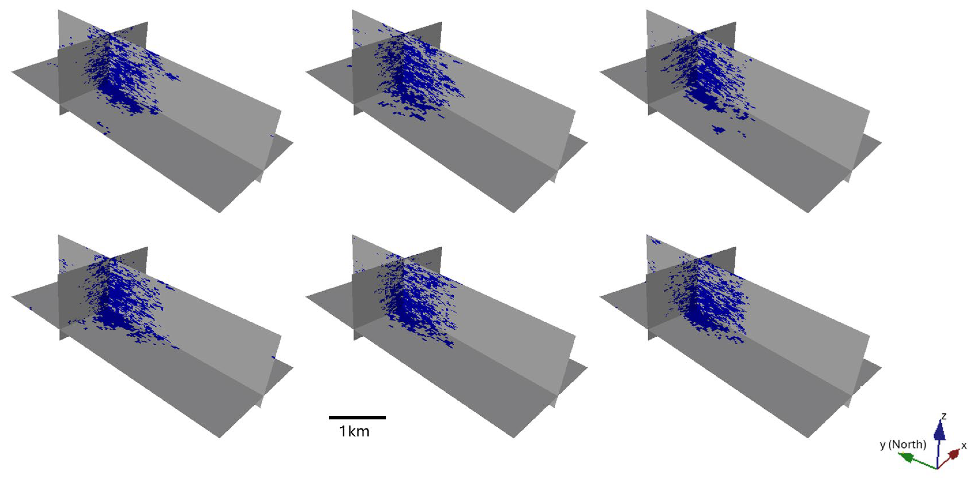
A few prior intrusion models for A3 can be seen in Figure 8. Early-stage simulation artifacts may be present but are not expected to significantly affect the determination of an optimal drilling strategy. The goal is not to produce fully accurate resource models, but to span plausible uncertainty ranges and capture relationships applicable to the undrilled area.

Figure 8. Prior models of intrusion obtained by co-SISIM.

Once the prior intrusion models have been generated, the next step is to populate these models with Ni grade values.

4.2.2. Geochemical Soil Samples to Inform Ni Grade

Our assumption is that the presence of Ni in the soil samples is an indication of Ni grade in the intrusion, at least in shallow areas. The training set is derived from A1, where both geochemical data and the Ni grade model are available.

In A1, a grade model was constructed by dividing the subsurface into 100-m-thick layers from the surface downward. Within each layer, Ni grades were estimated using an RBF interpolation [23] of the available drillhole data in 3D.

We propose to explore the available soil geochemistry data to guide the modeling of Ni grade in A3. Nickel and iron often occur together in ultramafic rocks. Fe is often abundant and commonly used in log ratios. The log(Ni/Fe) ratio helps normalize the concentration of nickel to that of iron, which is less mobile in many weathering environments. Thus, using the log ratio Ni/Fe ratio from soil samples may serve as a more reliable indicator of mineralization, potentially helping to normalize for background lithological variations and highlight geochemical anomalies associated with Ni enrichment.

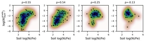
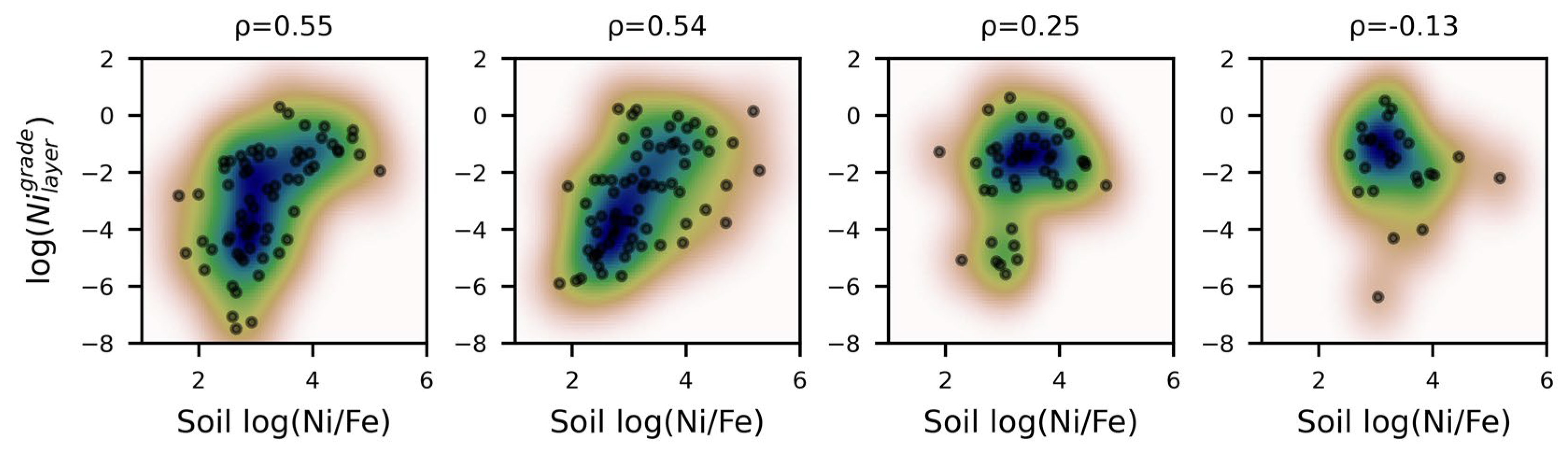
Figure 9 shows the relationship between $\log \left(N{i}^{soil}/F{e}^{soil}\right)$ in the soil samples and $\log \left(N{i}_{laye{r}_i}^{grade}\right)$ at $laye{r}_i$ in the grade model as a function of depth for A1. For shallow depths (0 to 200–300 m), some correlation is observed (about 0.55 for 0 to 200 m, 0.25 for 200–300 m). For deeper depths, the correlation becomes nonexistent. Hence, after a certain depth, the surface geochemistry cannot predict the Ni grade.

Figure 9. Scatter plot between $\log \left(N{i}_{laye{r}_i}^{grade}\right)$ and $\log \left(N{i}^{soil}/F{e}^{soil}\right)$ for 100 m-thick layers (from shallow to deep). The background represents the density estimation $f_{A1}$, obtained by Kernel Density Estimation (KDE).

Hence, statistical learning model consists of two components based on the depth of the modeled layers:

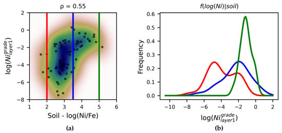
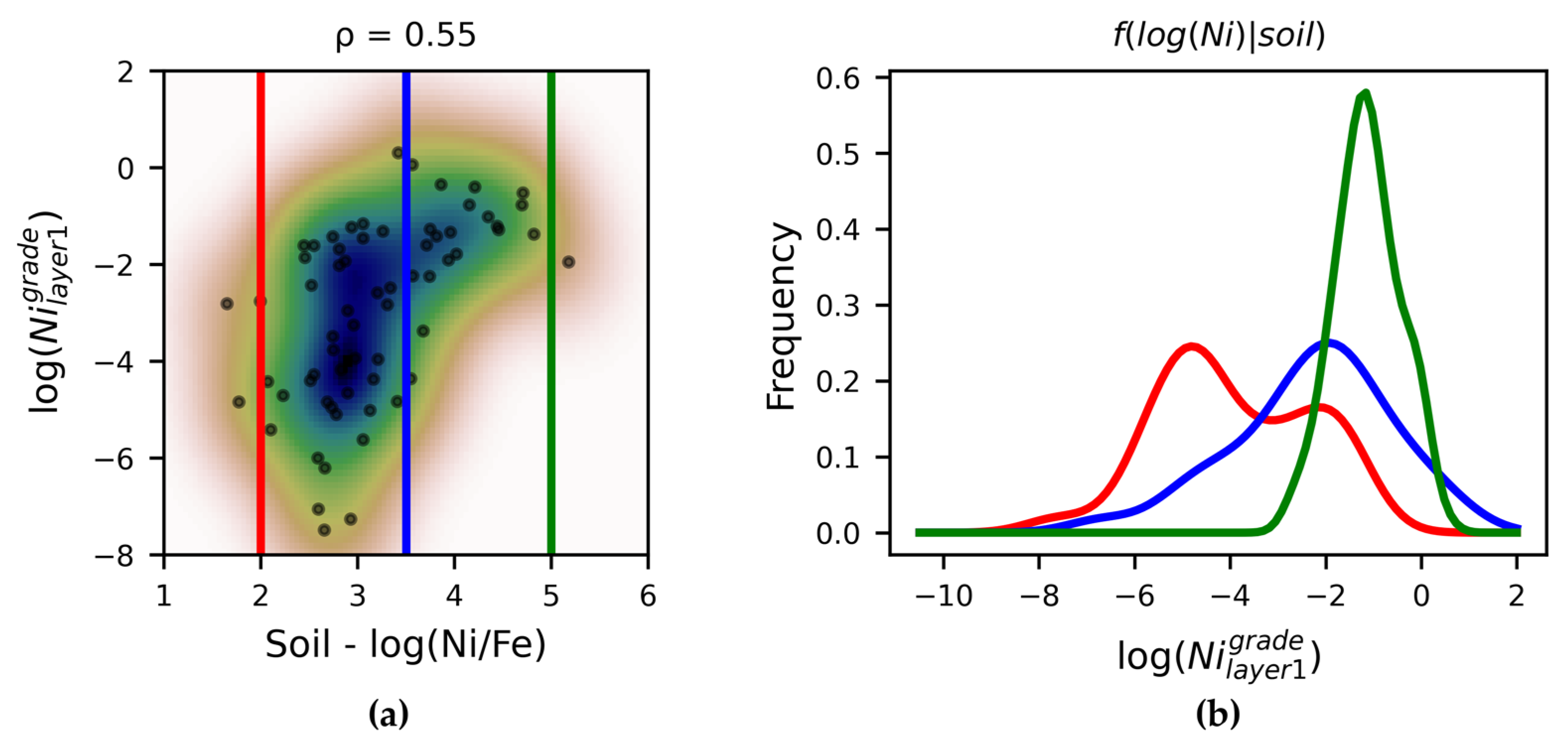
• Shallow layers (top three layers, i.e., top 300 m): For each of these layers, a bivariate probability density function (PDF) is estimated from A1 data to characterize the joint distribution between the log of Ni grade and the log of the Ni/Fe ratio in soil samples, see Figure 10:

  $$f_{A1}\left(\log \left(N{i}_{laye{r}_i}^{grade}\right),\log \left(N{i}^{soil}/F{e}^{soil}\right)\right)$$

  (5)
  

  Figure 10. (a): 2D scatter plot of soil samples $\log \left(N{i}^{soil}/F{e}^{soil}\right)$ and $\log \left(N{i}_{laye{r}_i}^{grade}\right)$ for layer₁. (b) Conditional densities of $\log \left(N{i}_{laye{r}_i}^{grade}\right)$ given soil samples values at the locations highlighted on the scatter plot.
• Deeper layers: Since soil geochemical signals become less relevant with depth, the Ni grade distribution in deeper layers is modeled using only the marginal prior distribution of the Ni grade for deeper layer, derived from A1: $f_{A1}\left(\log \left({Ni}^{grade}\right)\right)$.

Samples of Ni grade are generated using P-field simulation with the following PDF:

$$f(\log \left(N{i}_{laye{r}_i}^{grade}\right)|\log \left({\displaystyle \frac{N{i}^{soil}}{F{e}^{soil}}}\right))= \{\begin{array}{cc}{f}_{A1}\left(\log \left(N{i}_{laye{r}_i}^{grade}\right)\right|\log \left({\displaystyle \frac{{Ni}^{soil}}{{Fe}^{soil}}}\right))& for layer 1, 2 and 3\\ f_{A1}\left(\log \left({Ni}^{grade}\right)\right)& for layers>3\end{array}$$

(6)

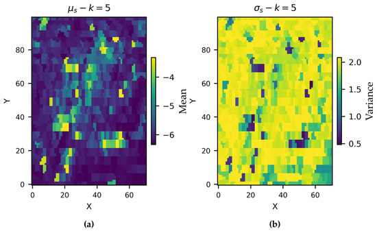
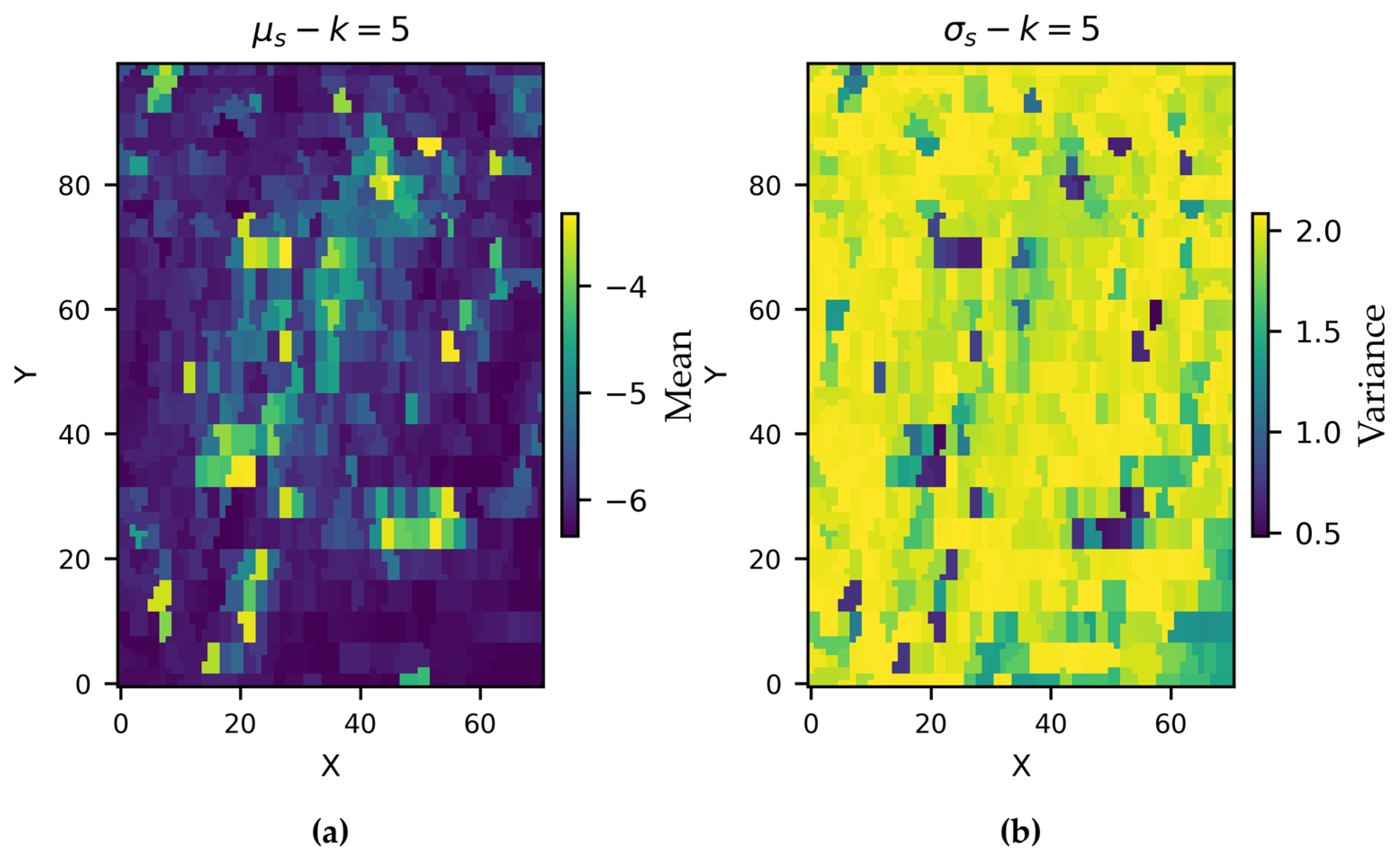
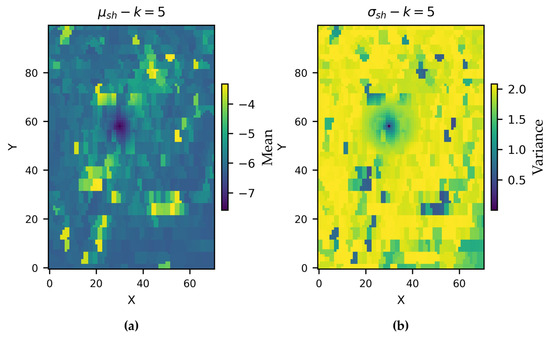
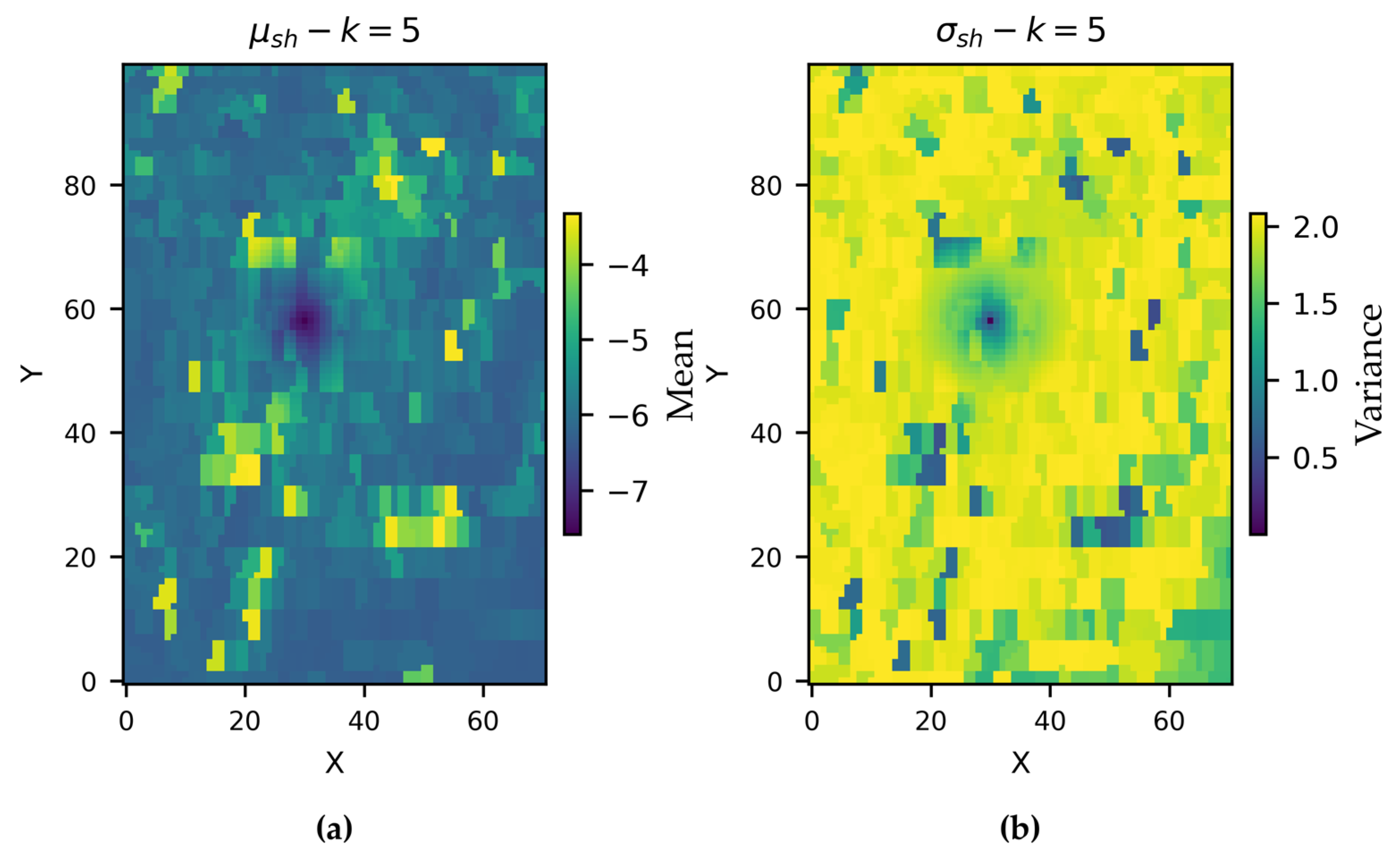
To make the simulation faster, the shallow part of the distribution $f \left(\log \left(N{i}_{laye{r}_i}^{grade}\right)|\log \left({\displaystyle \frac{N{i}^{soil}}{F{e}^{soil}}}\right)\right)$ is approximated by a Gaussian distribution, with spatially varying mean ${\mu }_{s,k}$, and standard deviation ${\sigma }_{s,k}$ for a depth of k, as shown in Figure 11.

Figure 11. (a) mean and (b) standard deviation of the local (Gaussian) CCDF for the soft data-derived PDF in the first layer (k = 5).

For the grade model, the p-fields were generated with a Spherical variogram with varying ranges as shown in Table 1:

Table 1. Variogram parameters in p-field simulations for grade modeling.

Variogram Ranges	Distribution	Min	Max
Range_x	U	5	20
Range_y	U	5	20
Range_z	U	5	10

For each grid cell in shallow layers, the closest soil sample is used to condition the local distribution. The log(Ni) grade is then sampled from the corresponding conditional cumulative distribution function (CCDF), using the value from the P-field realization.

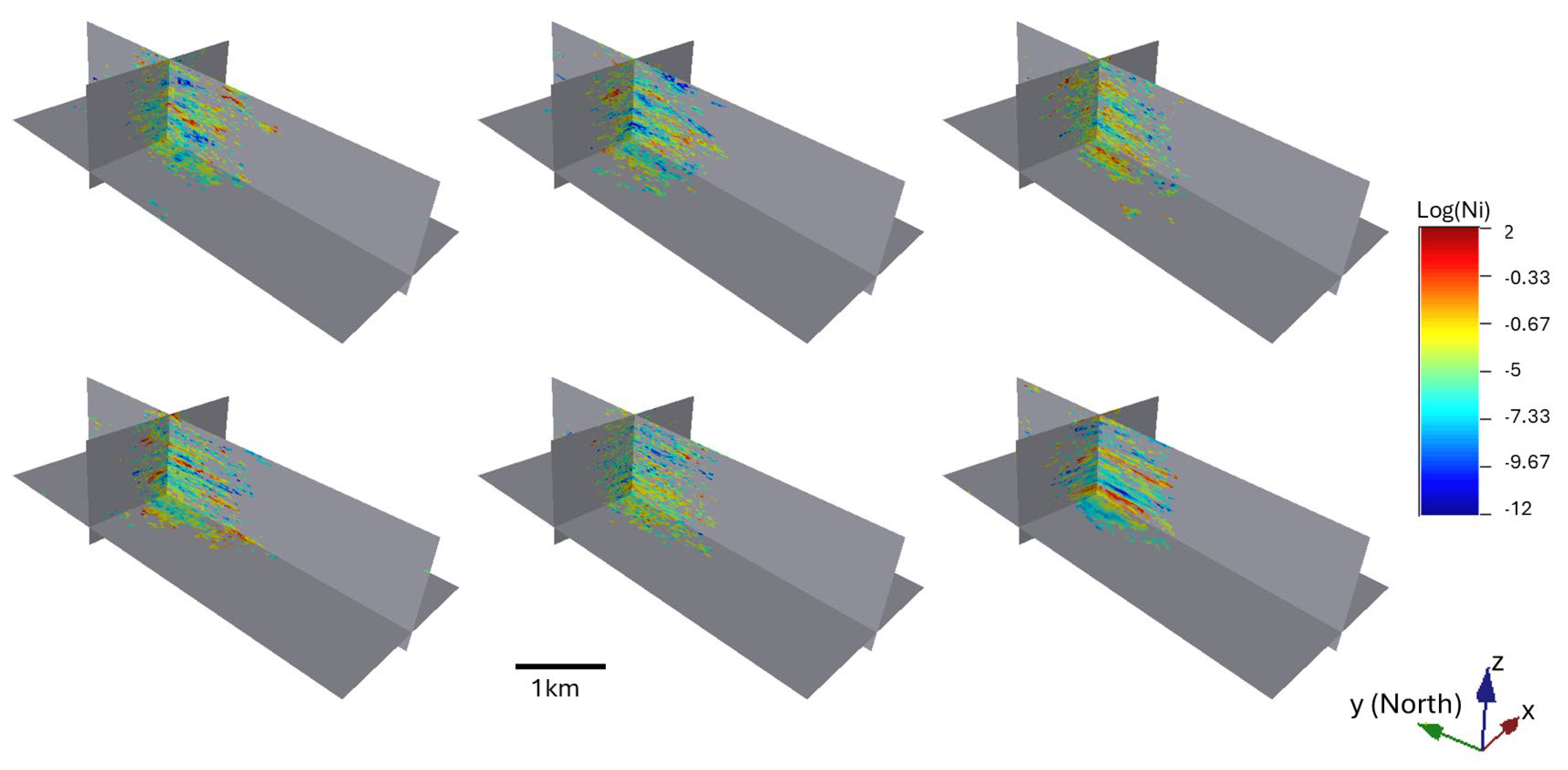
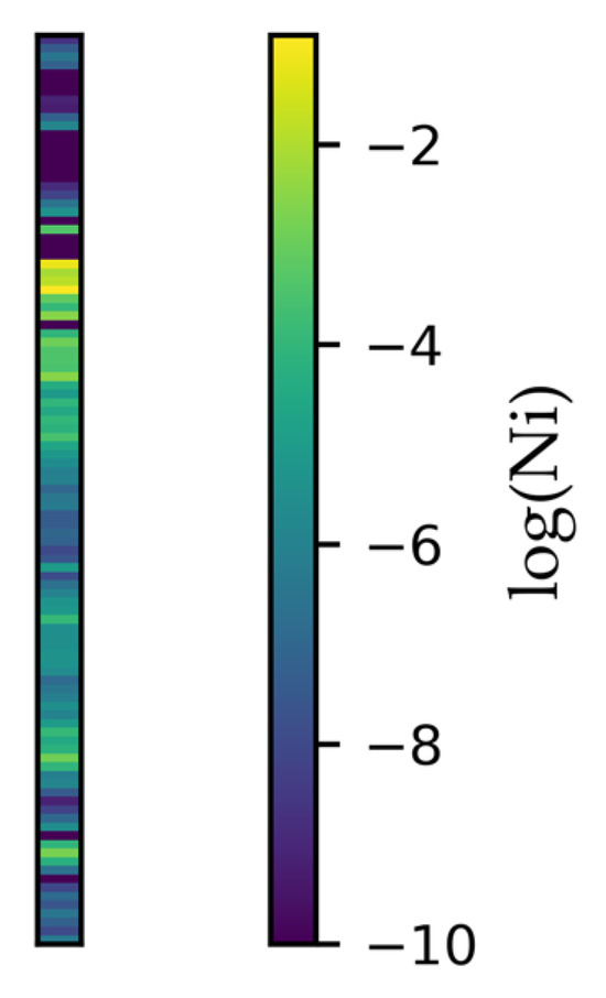
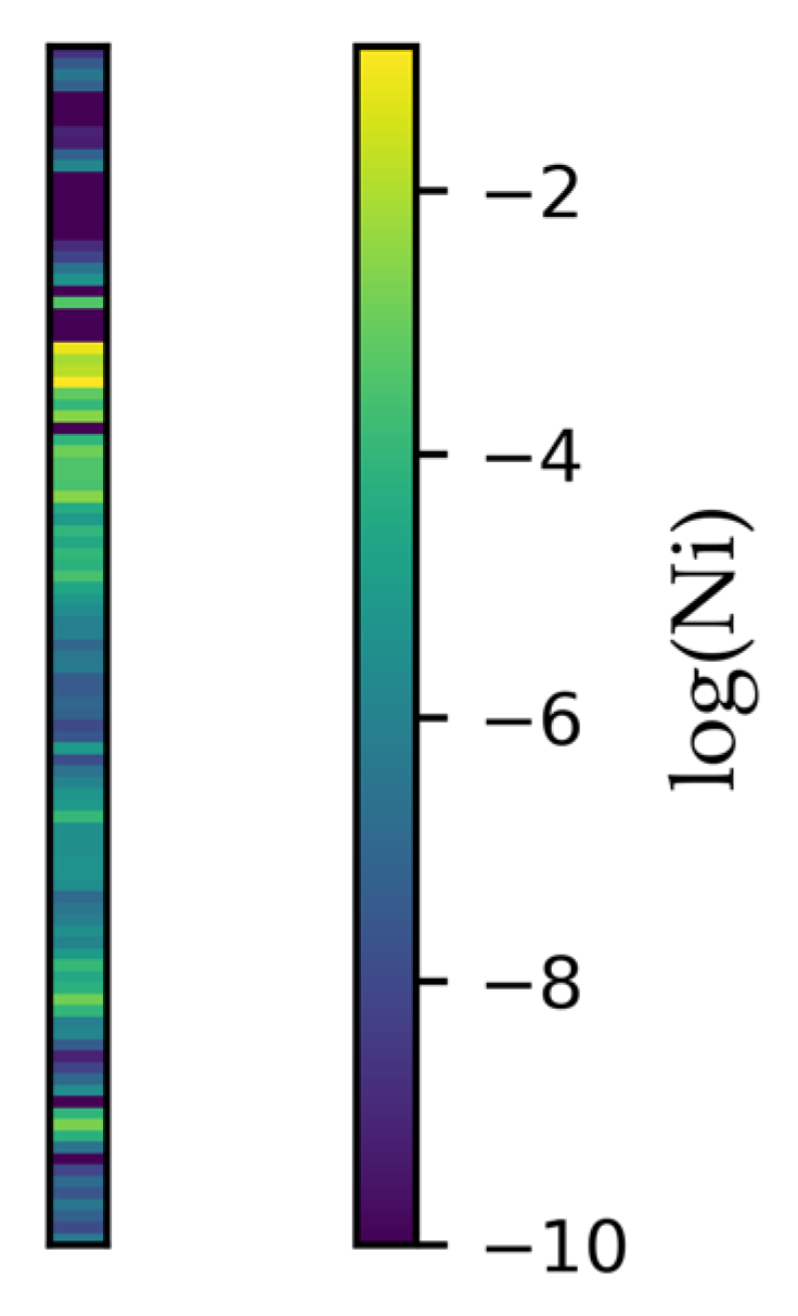
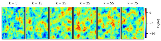
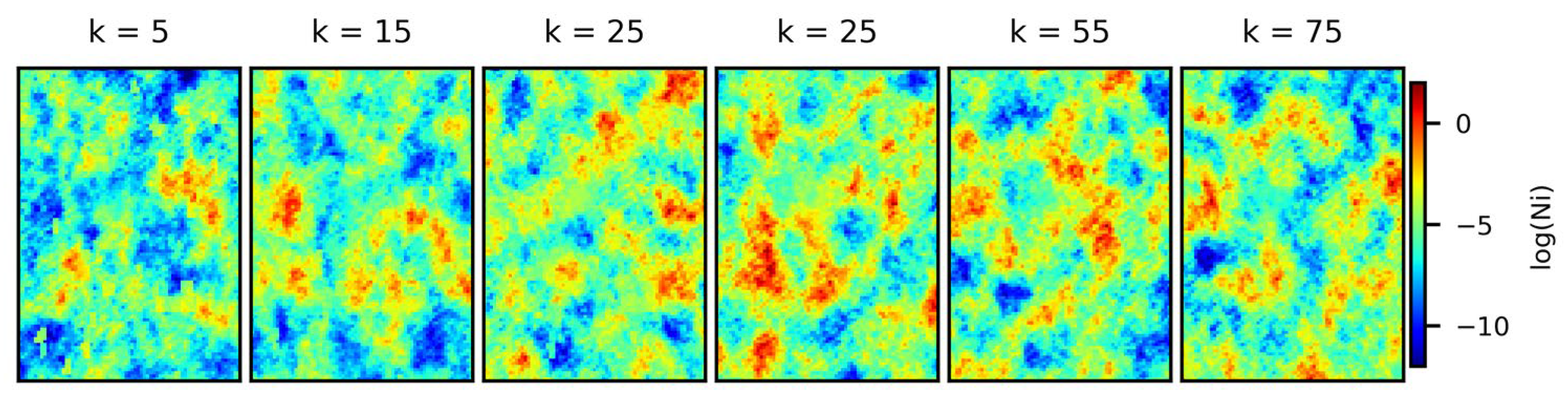
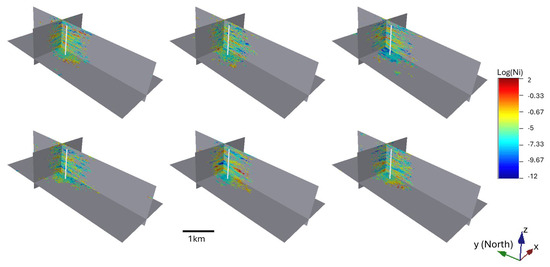
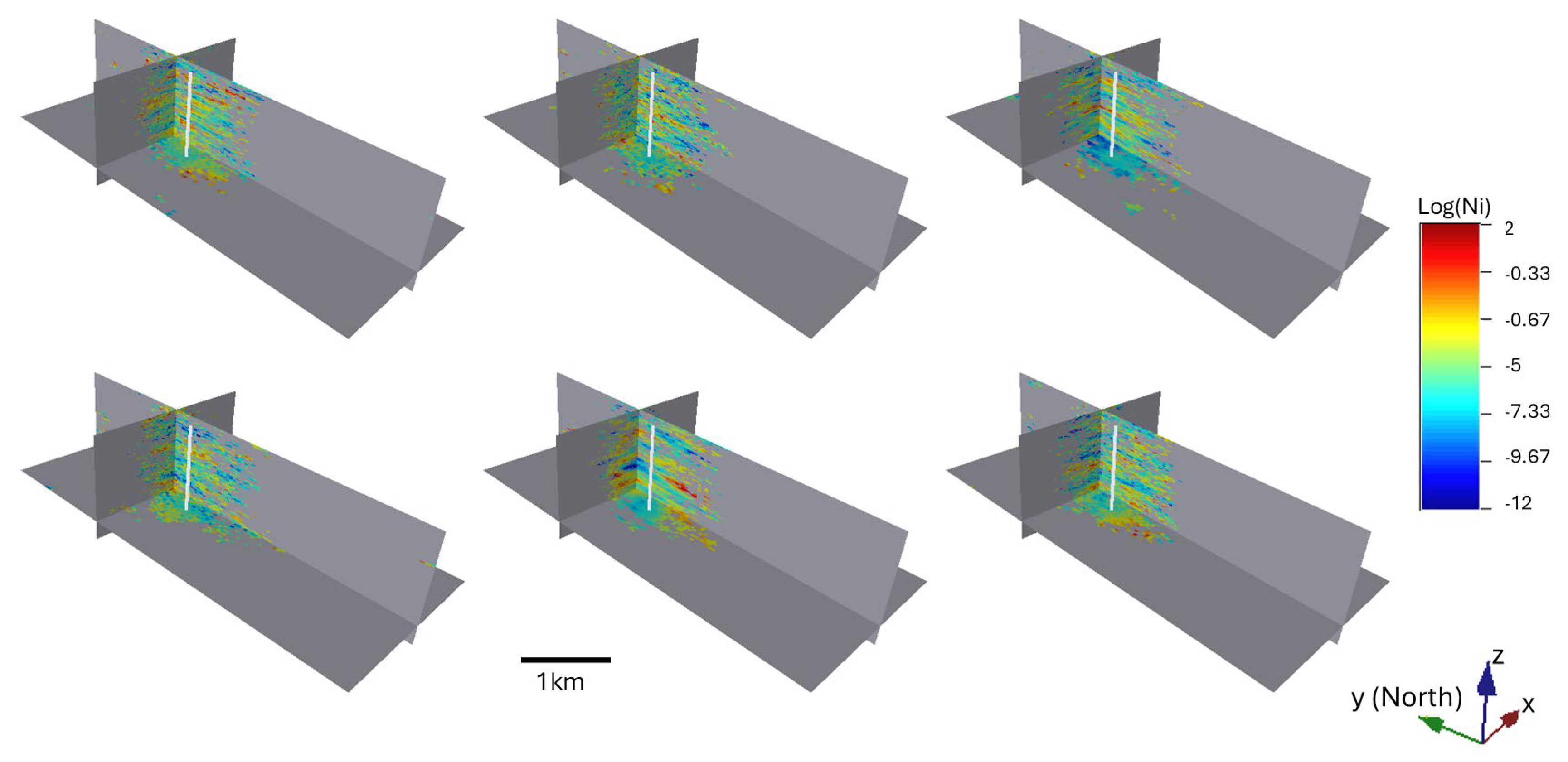
The final Ni grade model is constructed using a cookie-cutter approach. For each grid cell, if the corresponding intrusion model indicates the presence of intrusion, the Ni grade is assigned from the simulated grade model. Conversely, if the intrusion is absent in that cell, the Ni grade is set to zero. This masking procedure ensures that grades are only assigned within intrusion. A large set of equiprobable prior models of Ni grade can be generated; a few are shown in Figure 12. It is important to emphasize that the objective is not to construct accurate resource models, but rather to span uncertainty in order to support informed decision-making regarding drillhole placement.

Figure 12. A few prior models of log-Ni grade obtained by the proposed procedure.

4.3. EOI for Optimal Drilling

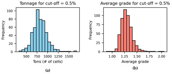
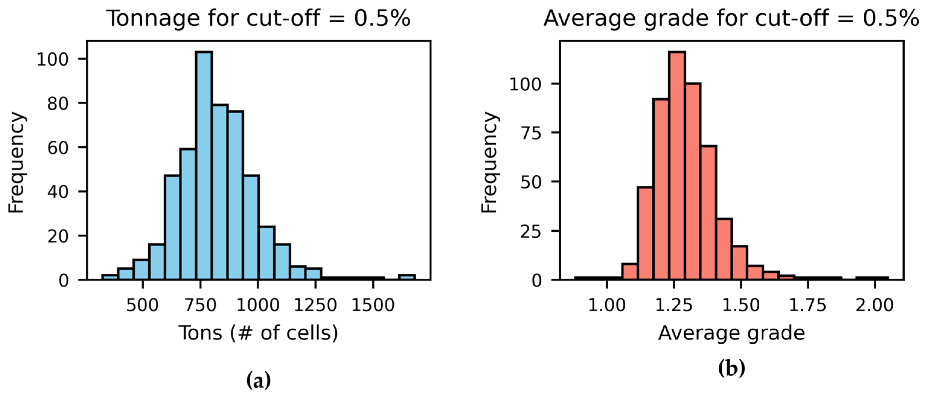
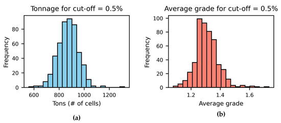
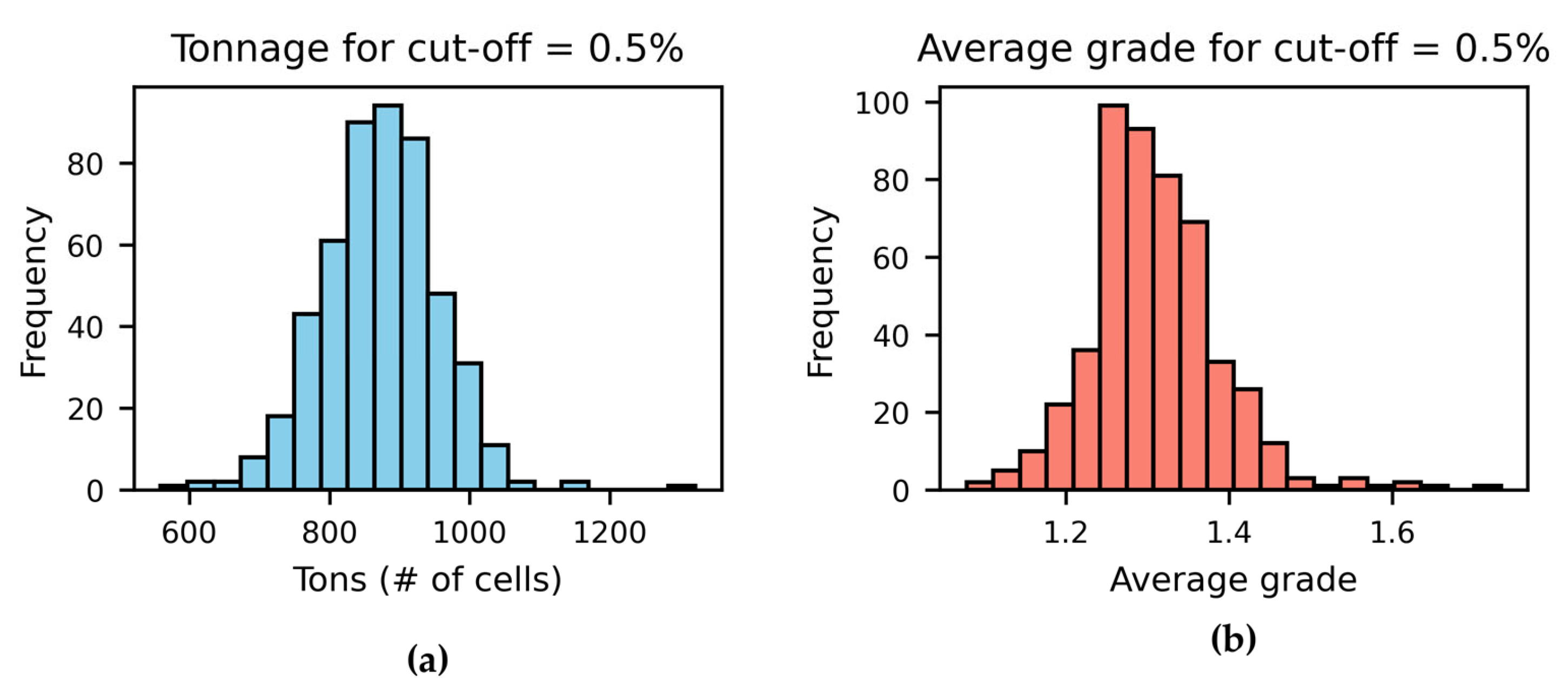
The next step is to apply EOI to define an optimal drilling sequence in A3. Our reward consists of both grade and tonnage as a function of a grade cut-off. The prior distribution of the reward can be directly computed by the set of prior models generated, as shown in Figure 13.

Figure 13. Prior rewards: (a) tonnage; (b) average grade for a cut-off of 0.5% and 500 prior models.

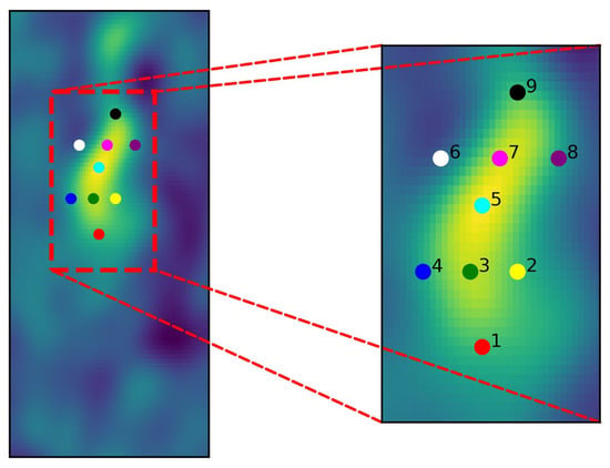
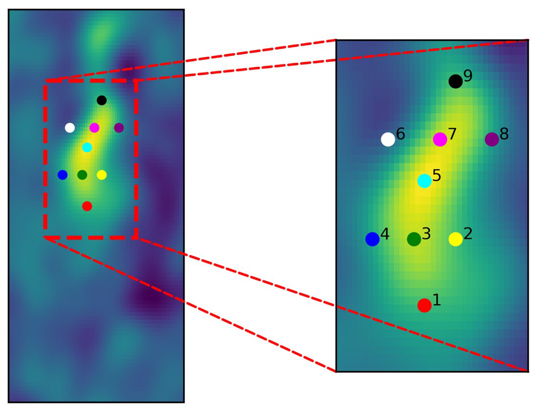
For this study, we proposed 9 candidate drillholes, located in or near the high-density area, see Figure 14. The drillholes are 105 pixels or 1050 m deep (they reach the bottom of the grid).

Figure 14. Drillhole location with respect to the density model for layer #15.

EOI is computed individually for each of the nine candidate drillholes. For each drillhole, the data $d^{\left(\mathcal{l}\right)}, \mathcal{l}=1,\dots ,L$ are extracted from the prior realizations by “drilling into” the realization, i.e., by extracting the Ni grade along the corresponding drillhole trajectory. This process provides the grade profiles that would be observed if the realization were the true subsurface.

To reduce the dimensionality of the data, kernel principal component analysis (KPCA) was applied using the Manhattan distance metric. The kernel bandwidth was chosen to preserve the effective similarity scale induced by the Manhattan distance, ensuring comparable kernel decay across realizations. Only the first few dimensions contributed significantly to the variance, allowing KPCA to reduce the data dimensionality to 3 from 105. In the reduced space, the density $f(\mathit{\theta }|d^{\ast \left(\mathcal{l}\right)})$ is estimated directly using a kernel density estimator, avoiding the need for computationally expensive model inversion. The posterior density is then compared to the prior density $f\left(\mathit{\theta }\right)$ via the Kullback–Leibler (KL) divergence. The procedure is repeated for all observations $d^{\ast \left(\mathcal{l}\right)}, \mathcal{l}=1,\dots ,L$ and the final EOI for a given drillhole is defined as the average KL divergence across all realizations (Equation (3)).

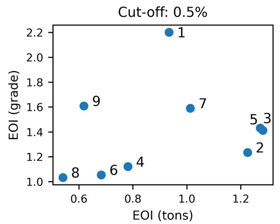
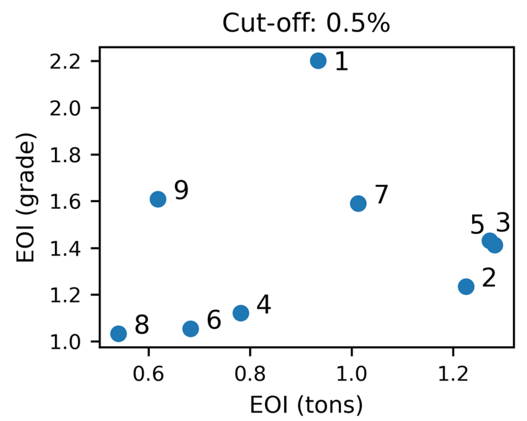
The results of the EOI analysis are presented in Figure 15. Drillholes #1, #7, #3 and #5 form an efficient frontier (Pareto front) and are identified as the most informative with respect to both grade and tonnage, based on a Ni grade cut-off of 0.5%. Holes #1, and to a lesser extent #7 and #9, are the most informative with respect to grade only and are located along the uncertain boundary defined by the density model, suggesting that this area is critical for reducing grade uncertainty. Holes #2, #3, and #5, located within the high-density region, contribute most significantly to reducing uncertainty in tonnage.

Figure 15. EOI for both tonnage and grade for a grade cut-off = 0.5%.

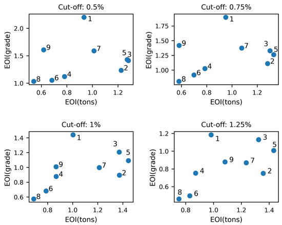
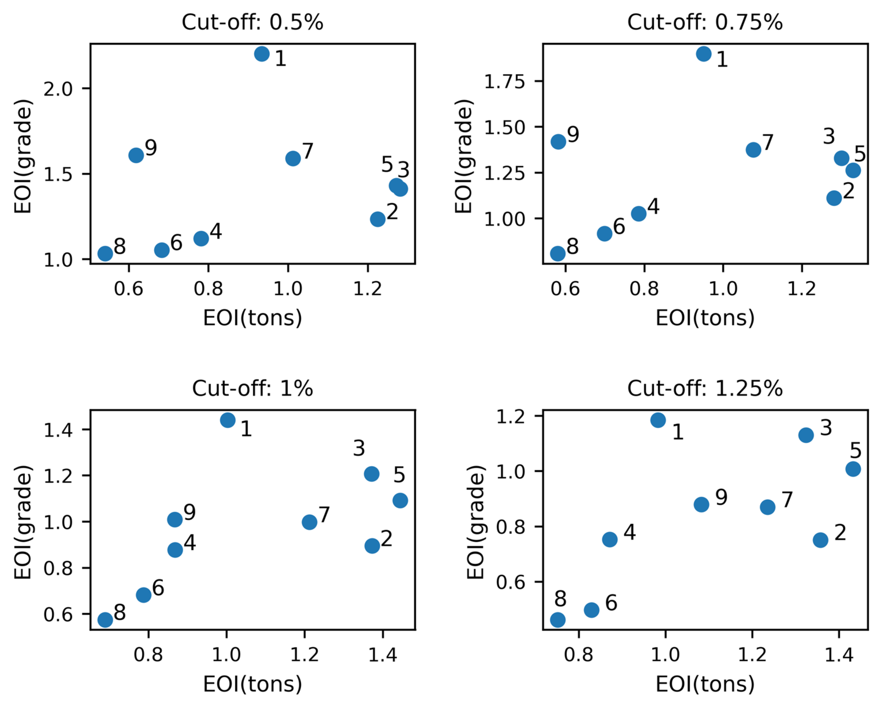
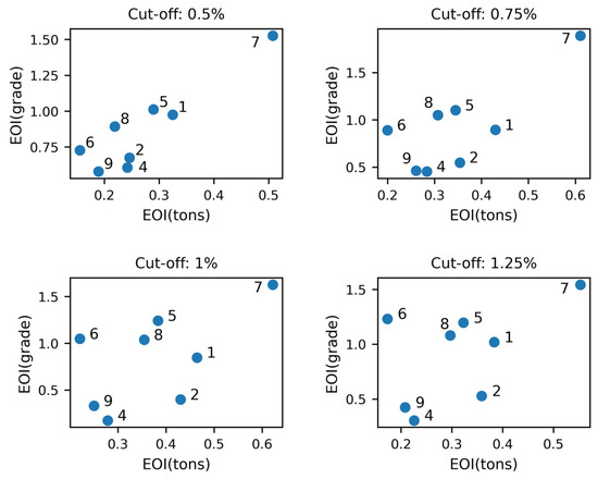
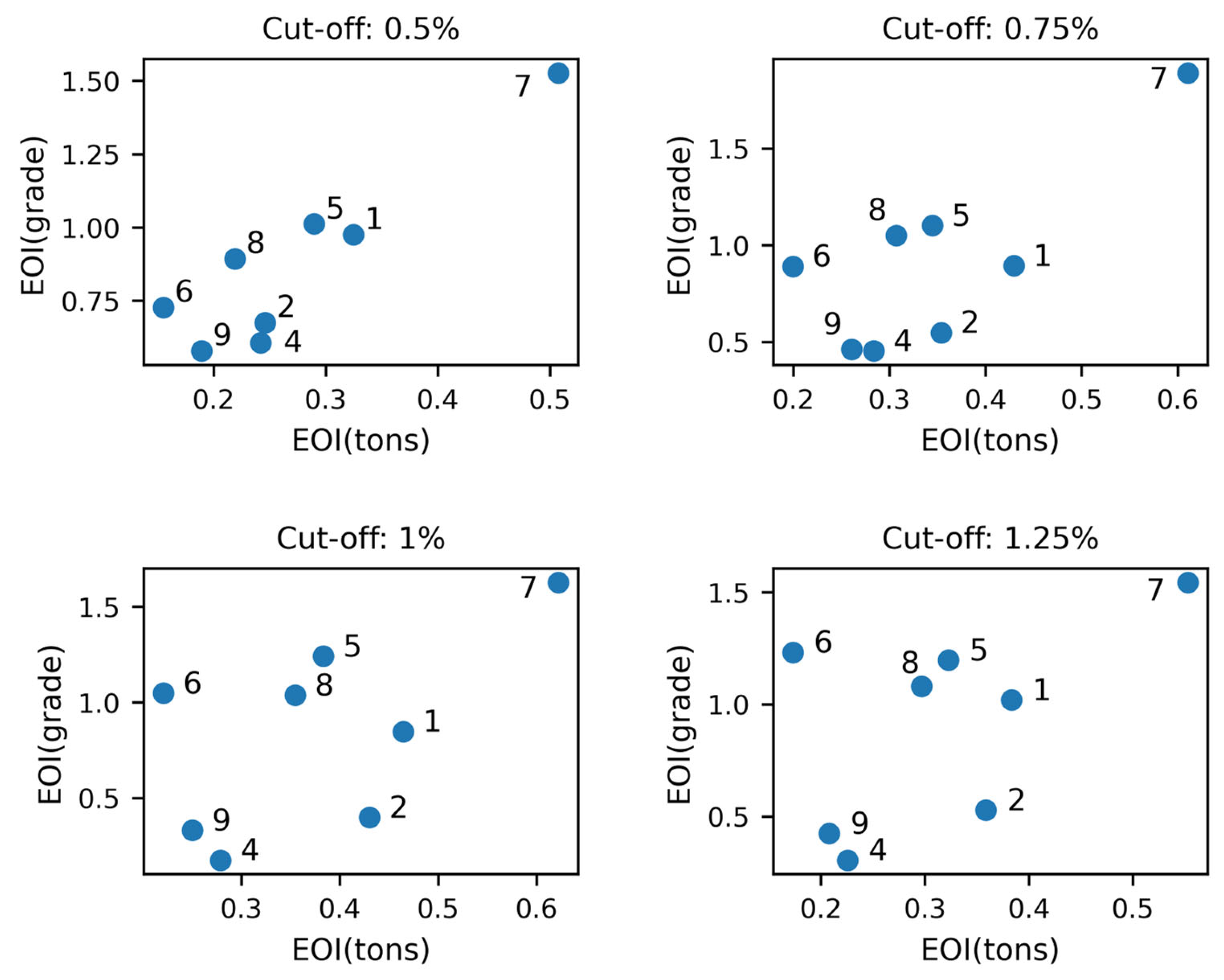
To assess the sensitivity of the optimal drillhole selection to the grade cut-off, the EOI procedure was repeated for multiple cut-off values, as shown in Figure 16. For most tested thresholds, and particularly at higher cut-off grades, drillhole #3 provides a high information gain with respect to both grade and tonnage. Ultimately, the selection of which hole to drill should be guided by the user’s specific objectives, whether the priority is to reduce uncertainty in tonnage, in grade, or both.

Figure 16. EOI calculation at each candidate borehole for grade and tonnage as a function of the grade cut-off.

In this study, drillhole #3 was selected for further analysis, as the objective was to prioritize reducing uncertainty on both grade and tonnage. Since actual drilling data are not available, one of the prior realizations was arbitrarily selected to serve as the “true” subsurface model. The synthetic observed data extracted along drillhole #3 from this realization are presented in Figure 17 and are denoted ${\mathit{d}}_{\mathit{o}\mathit{b}\mathit{s}}$.

Figure 17. Synthetic observed data (log(Ni) grade) extracted along drillhole #3.

The next step is now to generate models conditioned to that observation.

4.4. Conditioning with the Observed Data

4.4.1. Construction of Conditional Grade Model

When generating the prior models, the Ni grade was sampled using p-field simulation with local CCDF based on soft data only (pdf generated from soil samples, see Equation (6)). When new drilling data becomes available, the grade and intrusion model should additionally be constrained to the hard data (the grade at the drillhole location). This introduces the need to sample from a mixture of two distributions: the soft data-derived PDF and a hard data-derived PDF.

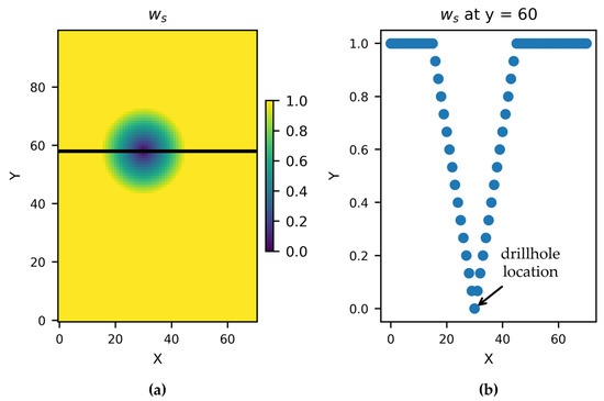
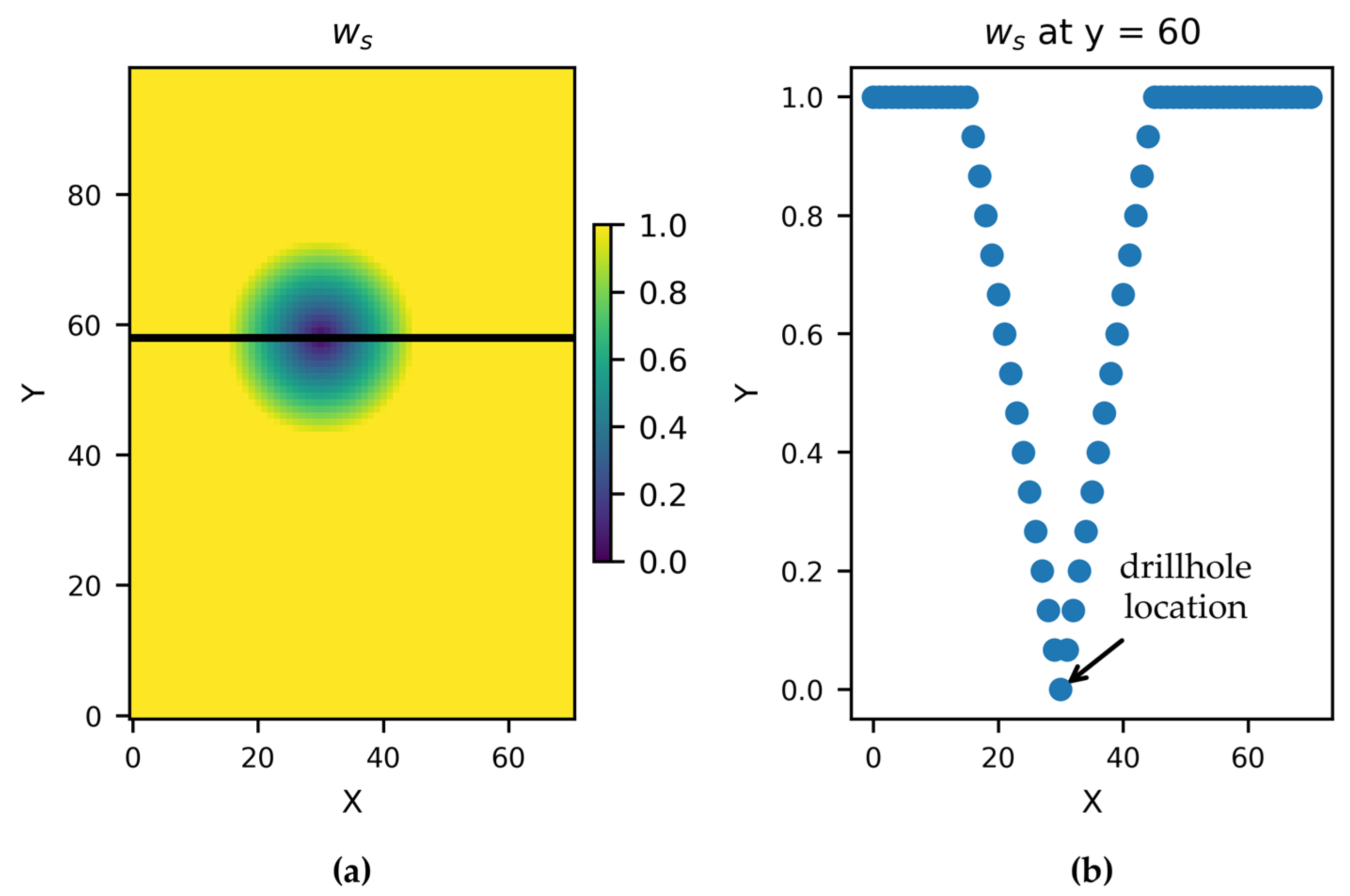
To appropriately balance the influence of each data source, we propose a distance-based weighting scheme. When simulating a grid cell located in close proximity to a conditioning drillhole, the simulation should prioritize consistency with the hard data, as it provides the most reliable local constraint. Conversely, for grid cells farther away from the drillhole, the influence of the hard data diminishes, and the simulation should rely more heavily on the geochemical (soft) data.

The local CCDF for conditional p-field simulation is thus defined as a weighted average of the hard and soft distributions. The weighting is a (linear) function of the distance between the simulation location and the conditioning drillhole, allowing for a smooth transition between local hard data conditioning and regional soft data influence. This approach enables the generation of spatially consistent grade realizations while honoring both local constraints and broader geochemical trends.

The resulting density if a function of depth k:

$$f_{cond}\left(\log \left(N{i}_k^{grade}\right)\right)= w_{s }f\left(\log \left(N{i}_{laye{r}_i}^{grade}\right)|\log \left({\displaystyle \frac{N{i}^{soil}}{F{e}^{soil}}}\right)\right)+\left(1- w_{s }\right)\ast f(\log \left(N{i}_k^{grade}\right)|{\mathit{d}}_{\mathit{o}\mathit{b}\mathit{s},\mathit{k}})$$

(7)

The $laye{r}_i$ is the 100 m-deep layer corresponding to the depth k. The weight $w_{s }$ is a function of the distance to the drillhole (see Figure 18). The first PDF defines the soft data-derived PDF and is the Gaussian approximation of the PDF in Equation (6) obtained from geochemical samples. The second PDF defines the hard data-derived PDF and can be modeled using a Gaussian distribution, with a mean equal to the observed data (at depth k: ${\mu }_{h,k}=$ $d_{obs,k}$) and a variance ${\sigma }_{h,k}$ proportional to the distance of the drillhole: near the drillhole, the variance is very small, hence samples will be close to the observed data, and will deviate gradually from it as we move away from the drillhole.

Figure 18. Spatial weight associated with the soft data-derived PDF: the farther from the drillhole, the higher the contribution of the soft data. (a) top view; (b) cross-section.

Because our model is a mixture of Gaussian fields, we can compute analytically the mean ${\mu }_{sh,k}$ and the variance ${\sigma }_{sh,k}^2$ of the mixture (shown in Figure 19):

$${\mu }_{sh,k}= w_{s }\ast {\mu }_{s,k}+\left(1-w_{s }\right)\ast {\mu }_{h,k}, k=1,\dots ,nz$$

(8)

$${\sigma }_{sh,k}^2=w_{s }\ast {\sigma }_{s,k}^2+\left(1-w_{s }\right)\ast {\sigma }_{h,k}^2+w_{s }\ast \left(1-w_{s }\right)\ast {\left({\mu }_{s,k}-{\mu }_{h,k}\right)}^2, k=1,\dots ,nz$$

(9)

Figure 19. (a) mean and (b) standard deviation of the local (Gaussian) CCDF for the soft data-derived PDF in the first layer (k = 5) for conditioning models to observed data.

P-field simulation can now be used in the same way to generate prior grade models using a defined distribution. An example of a conditional log(Ni) grade model at different depths can be seen in Figure 20.

Figure 20. Example conditional log(Ni) grade model as a function of depth.

4.4.2. Construction of Conditional Intrusion Models

We need to additionally constrain the intrusion model, which can be done in a similar way, using a mixture of two distributions: a soft data-derived PDF $f_{I,h}$ and a hard data-derived PDF $f_{I,h}$. The same weights $w_s$ are used:

$$f_I=w_s\ast f_{I,s}+\left(1-w_s\right)\ast f_{I,h}$$

(10)

The soft data-derived distribution $f_{I,s}$ is simply the probability of intrusion derived from Equation (4). The hard data-derived distribution $f_{I,h}$ has a value of 0 or 1 (depending on the absence/presence of intrusion at the drillhole) at the drillhole location and will increase/decrease to 0.5 as we move away from the drillhole. The resulting soft data cube (probability cube) is subsequently used in co-SISIM. Because the soft data incorporates conditional information, the resulting posterior realizations (see Figure 21) honor the hard data observed at the drillholes, particularly capturing the major vertical trends.

Figure 21. Updated log(Ni) grade realizations conditioned the drillhole.

The resulting posterior Ni-grade realizations match the observed data (both intrusion and grade, given a small error for the grade and intrusion) and can be used as new prior to applying a second EOI procedure to select the next drillhole to consider.

An updated distribution of tonnage and average grade can be computed, see Figure 22. Observations from Hole #3 indicate a decrease in tonnage and grade compared to the prior model predictions.

Figure 22. Updated rewards: (a) tonnage and (b) average grade for a cut-off of 0.5% and 500 updated models.

Applying the same EOI procedure to the updated models yields the next optimal set of drillholes, as shown in Figure 23. Hole #7 is clearly identified as the next optimal drillhole for both grade and tonnage. It should be noted, however, that the identified optimal location is conditional on the assumed true model and may differ if an alternative true model were considered.

Figure 23. 2nd EOI calculation at each candidate drillhole for grade and tonnage as a function of the grade cut-off.

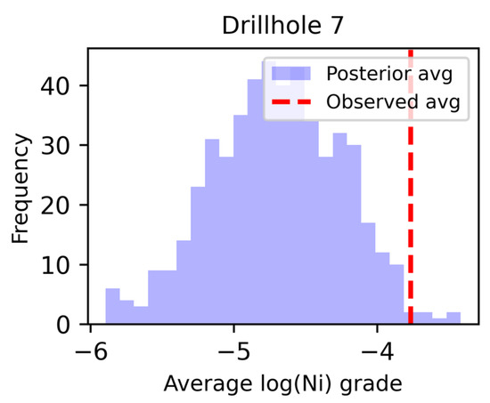
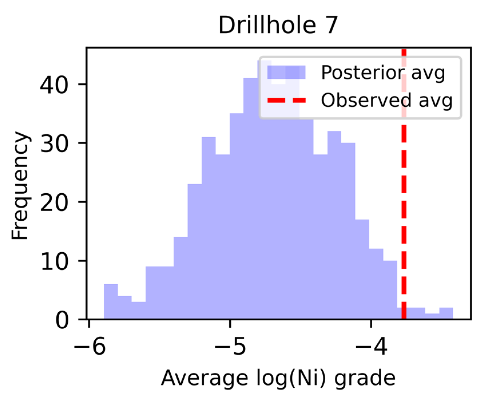
Although a full validation of the optimal drillhole selection is not feasible since it would require testing across many drillholes and multiple deposits, we can assess whether the updated uncertainty model (conditioned on observations from drillhole #3) is able to predict the subsequent drillhole (#7). This assessment is illustrated in Figure 24, which shows the distribution of the mean log(Ni) grade along drillhole #7 for all conditional models. The mean grade from the true model along drillhole #7 is indicated by the red line. As shown, the updated uncertainty model is consistent with the observed response of the new drillhole. While this does not constitute a formal validation, it demonstrates that the updated model cannot be falsified by the new observation.

Figure 24. Mean log(Ni) grade along drillhole #7. Distribution for the updated model of uncertainty and observed values from the true model.

5. Discussion

This study presents a drilling optimization framework designed for brownfield exploration, where data from previously explored areas is used to guide drilling in underexplored target areas. By learning statistical relationships between surface geochemistry, geophysical inversions, and models of intrusion and grade in well-characterized areas, an informed set of prior models can be generated in the new area despite the lack of drilling information. Rather than building a single, accurate resource model, the methodology focuses on modeling underlying uncertainty by generating an ensemble of prior realizations of grade and intrusion.

The use of the Efficacy of Information (EOI) allows to efficiently evaluate how informative alternative drilling options are, avoiding the need for full Bayesian inversion. Within this framework, “optimization” is understood as the systematic selection and ranking of candidate drillholes to identify those that are expected to be most informative. The drilling configuration with the highest EOI is most informative to reduce uncertainty on the specified reward. The case study in the Curaçá Valley, Brazil, demonstrates how prior geological knowledge from anomaly A1 can be transferred effectively to decide on the most informative locations to drill in the new area A3.

References

- Lindi, O.T.; Aladejare, A.E.; Ozoji, T.M.; Ranta, J.-P. Uncertainty quantification in mineral resource estimation. Nat. Resour. Res. 2024, 33, 2503–2526. [Google Scholar] [CrossRef] [Scilit]
- Li, S.-X.; Knights, P.; Dunn, D. Geological uncertainty and risk: Implications for the viability of mining projects. J. Coal Sci. Eng. 2008, 14, 176–180. [Google Scholar] [CrossRef] [Scilit]
- Rossi, M.E.; Deutsch, C.V. Mineral Resource Estimation; Springer: Dordrecht, The Netherlands, 2014. [Google Scholar] [CrossRef] [Scilit]
- Monteiro da Rocha, M.; Yamamoto, J.K. Comparison between kriging variance and interpolation variance as uncertainty measurements in the Capanema iron mine, State of Minas Gerais—Brazil. Nat. Resour. Res. 2000, 9, 223–235. [Google Scholar] [CrossRef] [Scilit]
- Liu, Y.; Carranza, E.J.M.; Xia, Q. Developments in quantitative assessment and modeling of mineral resource potential: An overview. Nat. Resour. Res. 2022, 31, 1825–1840. [Google Scholar] [CrossRef] [Scilit]
- Paithankar, A.; Chatterjee, S. Grade and tonnage uncertainty analysis of an African copper deposit using multiple point geostatistics and sequential Gaussian simulation. Nat. Resour. Res. 2018, 27, 419–436. [Google Scholar] [CrossRef] [Scilit]
- Fouedjio, F.; Klump, J. Exploring prediction uncertainty of spatial data in geostatistical and machine learning approaches. Environ. Earth Sci. 2019, 78, 38. [Google Scholar] [CrossRef] [Scilit]
- Mery, N.; Marcotte, D. Quantifying mineral resources and their uncertainty using two existing machine learning methods. Math. Geosci. 2022, 54, 363–387. [Google Scholar] [CrossRef] [Scilit]
- Afonseca, B.C.; Miguel Silva, V. Defining optimal drill hole spacing: A novel integrated analysis from exploration to ore control. J. S. Afr. Inst. Min. Met. 2022, 122, 305–315. [Google Scholar] [CrossRef] [Scilit] [PubMed]
- Hossein Morshedy, A.; Khorram, F.; Emery, X. A multi objective approach for optimizing the layout of additional boreholes in mineral exploration. Minerals 2023, 13, 1252. [Google Scholar] [CrossRef] [Scilit]
- Jafrasteh, B.; Suárez, A. Objective functions from Bayesian optimization to locate additional drillholes. Comput. Geosci. 2021, 147, 104674. [Google Scholar] [CrossRef] [Scilit]
- Aghlan, M.H.; Asghari, O.; Emery, X. Optimizing infill drill hole decisions while capturing the spatial continuity of geochemical and geometallurgical properties: Application to Gol Gohar iron ore mine, Iran. Minerals 2025, 15, 478. [Google Scholar] [CrossRef] [Scilit]
- Maleki, M.; Baeza, D.; Soltani Mohammadi, S.; Madani, N.; Díaz, E.; Anguita, F. Optimising the placement of additional drill holes to enhanced mineral resource classification: A case study on a porphyry copper deposit. Int. J. Min. Reclam. Environ. 2024, 39, 134–151. [Google Scholar] [CrossRef] [Scilit]
- Chen, C.; Fan, J.; Liu, H.; Guo, C.; Zhang, L.; Yuan, W.; Wang, K. Subsurface faults and magma controls on the Jinchuan Ni-Cu sulfide deposit: Constraints from magnetotelluric data. Minerals 2024, 14, 1080. [Google Scholar] [CrossRef] [Scilit]
- Hayward, N. Improving multi-scale structural targeting precision for large Ni-Cu (±PGE, Co) sulfide discoveries from global case studies. Econ. Geol. 2024, 119, 1745–1767. [Google Scholar] [CrossRef] [Scilit]
- Caers, J.; Scheidt, C.; Yin, Z.; Wang, L.; Mukerji, T.; House, K. Efficacy of information in mineral exploration drilling. Nat. Resour. Res. 2022, 31, 1157–1173. [Google Scholar] [CrossRef] [Scilit]
- Barnes, S.J. Lithogeochemistry in exploration for intrusion-hosted magmatic Ni–Cu–Co deposits. Geochem. Explor. Environ. Anal. 2023, 23, 1–17. [Google Scholar] [CrossRef] [Scilit]
- Ero Copper Corp. Ero Copper Announces Discovery of Nickel Sulphide System in the Curaçá Valley; Intercepts 16.5 Meters Grading 1.22% Nickel, Including 3.8 Meters Grading 3.60% Nickel. GlobeNewswire. Available online: https://www.globenewswire.com/news-release/2022/09/29/2529185/0/en/Ero-Copper-Announces-Discovery-of-Nickel-Sulphide-System-in-the-Curaca-Valley.html (accessed on 3 December 2025).
- Srivastava, R.M. Reservoir characterization with probability field simulation. In Proceedings of the SPE Annual Conference and Exhibition, Washington, DC, USA, 4–7 October 1992; pp. 927–938. [Google Scholar]
- Goovaerts, P. Geostatistics for Natural Resources Evaluation; Oxford University Press: Oxford, UK, 1997. [Google Scholar]
- Remy, N.; Journel, A.G.; Deutsch, C.V. Applied Geostatistics with SGeMS: A User’s Guide; Cambridge University Press: Cambridge, UK, 2009. [Google Scholar]
- Asadi, A.; Caers, J.; Mejia-Herrera, P.; Yin, Z. Exploration drill targeting based on similarity with known economical mineral deposits. Min. Met. Explor. 2025. submitted. [Google Scholar]
- Buhmann, M.D. Radial Basis Functions: Theory and Implementations; Cambridge University Press: Cambridge, UK, 2003; p. 272. [Google Scholar]
Disclaimer/Publisher’s Note: The statements, opinions and data contained in all publications are solely those of the individual author(s) and contributor(s) and not of MDPI and/or the editor(s). MDPI and/or the editor(s) disclaim responsibility for any injury to people or property resulting from any ideas, methods, instructions or products referred to in the content. |
© 2026 by the authors. Licensee MDPI, Basel, Switzerland. This article is an open access article distributed under the terms and conditions of the Creative Commons Attribution (CC BY) license.