


Abstract
Street cries are vocal expressions used by hawkers to advertise products or services in public spaces. Although they may reflect adaptation to noisy urban environments, their acoustic characteristics remain poorly understood. This study evaluated whether street cries (SC) differ acoustically from the hawkers’ normal speaking voices (NV) and whether these differences can be captured using compact feature subsets. Sixteen acoustic features related to fundamental frequency, formant structure, spectral properties, and voice quality were extracted. Redundant features were removed based on Kendall’s correlations, after which four classifiers were evaluated: support vector machine (SVM), random forest (RF), k-nearest neighbors (KNN), and Gaussian naive Bayes (GNB). Binary particle swarm optimization (BPSO) was then used for feature selection, with controlling the trade-off between cross-validated balanced accuracy and subset size. In repeated participant-grouped cross-validation, SVM achieved the highest mean balanced accuracy with the 13-feature vector (0.887 ± 0.056). On the held-out test set, BPSO-selected subsets yielded balanced accuracies of 0.783–0.900. The best SVM and GNB configurations both achieved 0.900 using six and four features, respectively. The features and appeared in all selected subsets. These results indicate that SC and NV can be differentiated using parsimonious, interpretable acoustic feature sets.
1. Introduction
For centuries, street cries have formed part of urban soundscapes in many regions of the world and remain a distinctive element of popular culture. Beyond their social and historical significance, these vocalizations may vary acoustically according to the environments in which they are produced. Their characteristic delivery often allows listeners to recognize that a product or service is being advertised even before fully processing the verbal content. Nevertheless, street cries have been studied primarily from historical, cultural, and socioeconomic perspectives [1,2,3].
Sharma [1] notes that urbanization and the growing prevalence of motorized traffic have increased ambient noise levels. Under these conditions, street vendors may need to produce louder or more projected calls to remain audible and attract potential customers.
In this context, street cries may be interpreted within the acoustic adaptation hypothesis, which has been widely studied in birds, mammals, insects, and anurans [4,5,6]. The vocal adjustments involved may serve two related functions: increasing the perceptual reach of the message and supporting commercial activity.
Acoustic parameters have been widely used to characterize phonatory processes, including vocal quality in individuals with voice disorders [7], differences between patients with and without depression [8], and differences between spoken and sung tasks [9]. However, the quantitative differentiation of street cries from the normal speaking voices of the same speakers remains largely unexplored.
The aim of this study was to determine whether street cries produced by hawkers in Mexico City exhibit quantifiable acoustic differences from their normal speaking voices and whether these differences can be captured using compact subsets of acoustic parameters.
To address this question, 16 acoustic parameters were initially extracted. A correlation-based reduction was then applied to remove redundant features, after which combinations of parameters were explored through feature selection and supervised classification. Four classifiers representing complementary learning strategies were evaluated: support vector machine (SVM), k-nearest neighbors (KNN), Gaussian naive Bayes (GNB), and random forest (RF). SVM constructs decision boundaries with a large generalization margin [10,11]; KNN provides a nonparametric, proximity-based approach [12]; GNB offers a simple probabilistic baseline that can remain competitive despite dependencies among features and deviations from normality [13,14]; and RF can model nonlinear relationships and interactions among variables [15,16].
Binary particle swarm optimization (BPSO) was used to identify compact feature subsets while balancing classification performance and parsimony [17,18]. Uniform Manifold Approximation and Projection (UMAP) was subsequently used as a post hoc descriptive tool to visualize the geometry of the selected feature spaces while approximately preserving neighborhood structure [19,20]. Overall, this framework was designed to evaluate the separability of street cries and normal speaking voices while preserving acoustic interpretability.
2. Theoretical Background
This section mentions the main theoretical foundations on which this research is based, ranging from the definitions of the acoustic variables used and the metrics to evaluate the performance of the classification, to the mathematical principles of the algorithms used in the optimization and visualization stages.
2.1. Acoustic Parameters
Acoustic parameters are quantitative metrics that allow us to evaluate different properties of signals such as voice. Among these parameters we find jitter, which is calculated the cycle-to-cycle period perturbations of successive glottal cycles during sustained phonation [21]. There are several ways to calculate jitter; one of them is local jitter, defined by the following Equation (1).
where denotes the extracted glottal periods and N the total number of periods [22]. Another helpful parameter for measuring disturbances is shimmer. This parameter assesses the perturbation of the amplitude of the sound wave across consecutive periods; that is, it quantifies the variability in intensity or energy between successive cycles of vocal fold vibration during speech [21]. It is calculated as shown in the Equation (2).
where are the extracted amplitudes and N is the number of periods obtained from the fundamental frequency [22].
On the other hand, a parameter that allows us to obtain information about the main source of the voice is fundamental frequency , also known as pitch, it is directly associated with the vibration of the vocal folds and corresponds to the number of times the glottis opens and closes within one second [21] expressed in Hz. Vocal folds of greater length tend to vibrate at a slower rate; nevertheless, additional factors including mass, thickness, tension, age, and sex also play a significant role. The standard deviation of the fundamental frequency () quantifies the temporal variability of throughout the vocal emission. While the fundamental frequency reflects the rate of vocal-fold vibration, provides information about the stability or fluctuation of this vibratory pattern over time. From an acoustic perspective, higher values indicate greater variations in fundamental frequency and, therefore, increased tonal variability during phonation. Conversely, lower values suggest a more stable and uniform vocal emission. In Praat, this descriptor is obtained as the standard deviation of the fundamental frequency points estimated within the analyzed time window. Thus, was used as a measure of pitch variability across the selected vocal segment. The pitch range quantifies the amplitude of variation in the fundamental frequency during vocal production. It was obtained as the difference between the maximum and minimum values of within the analyzed segment:
This descriptor summarizes the overall tonal extent of the voice signal. Thus, higher pitch range values indicate a greater excursion of over time, whereas lower values reflect a vocal production with more restricted tonal variability.
In the phonoarticulatory structure, some frequencies are favored by concentrating more energy, such as formants. These are the resonant frequencies of the vocal tract that generate regions of higher spectral intensity. They are commonly denoted as , , , ⋯, , ordered in ascending frequency. The pattern formed by the first formants (typically the first two) is largely responsible for the perceptual differences among vowels. Since longer vocal tracts exhibit lower resonances, the absolute frequencies of the formants depend on the size of the vocal tract [23]. Furthermore, formant dispersion is computed to quantify the frequency separation between pairs of formants. In Praat, for each audio file, formant frequency values are extracted frame by frame, and the absolute difference between each formant pair is calculated as . The final dispersion value is obtained by averaging these absolute differences across all valid frames. Frames containing missing or undefined values (NaN) in either of the two formants are excluded from the computation. Thus, provides a summary measure of the average spectral distance between two vocal-tract resonances over time.
A useful parameter for measuring the relationship between harmonicity and noise is the harmonic to noise ratio . It is an acoustic parameter of the voice used to evaluate vocal quality, as it quantifies the ratio between the harmonic or periodic components and the noise or aperiodic components of the signal, expressed in decibels (dB). A higher indicates a clearer, higher-quality voice, while a lower is associated with increased turbulent noise, hoarseness, and vocal cord dysfunction [24,25]. Mathematically, a voice signal with a harmonic structure in the frequency domain can be expressed by the Equation (4)
where X (w) corresponds to the speech signal in the frequency domain, H (w) to the harmonic component and N (w) to the noise component.
is a logarithmic measure of the energy ratio that is associated with the harmonic and noise component. Using the Equation (5) it is possible to integrate the spectral power over the audible range of frequencies [25]
The standard deviation of the harmonic to noise ratio quantifies the temporal variability of the harmonic-to-noise balance throughout the vocal signal. While measures the relative dominance of the harmonic component over the noise component, describes how stable or variable this relationship remains over time. Because is also expressed in dB, higher values indicate greater fluctuations in the harmonic-to-noise ratio across the analyzed segment, suggesting a less stable balance between periodic vocal-fold vibration and noise-related components. Conversely, lower values reflect a more consistent harmonic-to-noise structure during vocal production.
Focusing on the voice signal spectrum, center frequency is obtained from the power spectrum parameterization performed with FOOOF (Fitting Oscillations and One-Over-F) in Python. This framework models the power spectrum as the combination of an aperiodic component, which captures the broadband -like spectral background, and a periodic component, which represents peaks of power above that aperiodic background. These peaks are interpreted as putative oscillatory components within the analyzed frequency range. In the FOOOF model, each periodic peak, indexed by n, is parameterized by fitting a Gaussian function of the form:
where F denotes the array of frequency values, a represents the height of the peak, over and above the aperiodic component, c corresponds to the center frequency of the peak, and w describes the width of the peak [26]. In this study, the center frequency () was defined as the frequency location of the most prominent periodic peak detected by FOOOF, selected as the peak with the highest power above the aperiodic component. Thus, indicates the frequency at which the strongest putative oscillatory component of the amplitude-envelope spectrum is centered.
The power parameter is obtained from the periodic component estimated by FOOOF. In this model, periodic activity is represented as peaks of power above the aperiodic spectral background, with each detected peak parameterized by a Gaussian function. Within this parameterization, corresponds to the height of the Gaussian peak relative to the aperiodic component. In this study, was defined as the peak height of the most prominent periodic component detected in the amplitude-envelope power spectrum. Specifically, when multiple peaks were identified by FOOOF, the peak with the highest power was selected, and its corresponding height was stored as . Therefore, provides a measure of the strength of the dominant putative oscillatory component above the -like spectral background.
In spectral parameterization, the aperiodic component describes the broadband background of the power spectrum, that is, the portion of the spectrum that is not represented by narrowband periodic peaks. In this sense, aperiodic activity refers to spectral structure without a specific characteristic frequency or rhythmic peak. The α exponent parameter is obtained from the aperiodic component estimated by FOOOF, which models this aperiodic background using an exponential-like function in semi-logarithmic space. In the knee formulation, the aperiodic fit can be expressed as
where F denotes the array of frequency values, b represents the broadband offset, k is the knee parameter, and corresponds to the exponent of the aperiodic fit [26]. In the fixed mode, where no knee parameter is estimated, the aperiodic component is commonly represented as a linear trend in log-power space, and the exponent describes the rate at which power decreases as frequency increases.
In this study, corresponds to the aperiodic exponent returned by FOOOF. This parameter summarizes the slope of the broadband spectral background: larger exponent values indicate a steeper decrease in power across frequency, whereas smaller values indicate a flatter aperiodic spectrum. Thus, the exponent was used as a descriptor of the non-periodic spectral structure of the amplitude-envelope power spectrum.
2.2. Classification Performance Metrics
SC was considered the positive class and NV the negative class for the classification performance metrics.
Accuracy is a metric that provides the proportion of correctly predicted classifications over the total number of instances [27,28], that is:
where are the positive instances correctly predicted as positive, the negative instances correctly predicted as negative, the negative instances incorrectly predicted as positive (Type I error), and the positive instances incorrectly predicted as negative (Type II error).
Balanced accuracy metric calculates the arithmetic mean of sensitivity (proportion of positive cases correctly identified, also known as true positive rate (TPR)) and specificity (proportion of negative cases correctly classified, also known as true negative rate (TNR)) [29,30]. Therefore, balanced accuracy is calculated as:
The precision metric is the fraction of positive predictions that were correct for a class k, that is:
The weighted average precision is computed by weighting the precision of each class according to its support, that is, the number of true instances belonging to that class, as shown in Equation (11).
where denotes the support of class k, N is the total number of samples, and is the precision obtained for class k.
Recall (also referred to as sensitivity) is the proportion of all truly positive instances that the model correctly predicted for a class k. It is defined as:
F1 score is defined as the harmonic mean of precision and recall. Because this does not consider the ratio of negative instances correctly predicted by the classifier, two models with different specificity could have the same F1 score [30]. The equation to calculate it is as follows:
Another highly useful tool is the ROC curve (Receiver Operating Characteristic) for evaluating performance in binary classification. In this study, it corresponds to one class versus the other. The ROC curve is a plot of sensitivity against (1 − specificity). The term (1 − specificity) is also known as the false positive rate (), which identifies the proportion of negative cases classified as positive (14). For this plot, the AUC measure is used, corresponding to the area under the ROC curve, with values ranging from 0 to 1. A value of 0.5 indicates that the test has no discriminative power, representing a completely random case, whereas a value of 1 indicates perfect discriminative ability [27,28,31].
2.3. Particle Swarm Optimization
Particle Swarm Optimization (PSO), originally proposed by Kennedy and Eberhart in 1995, is a population optimization algorithm inspired by the collective behavior and swarm intelligence of flocks of birds and schools of fish. Under this approach, each particle represents a candidate solution within a search space of dimension D. These particles have two main characteristics: a position and a velocity, and their movement is guided by both their individual best experience and the best solution found by the swarm. In its classical form, the update is expressed as:
where denotes the velocity of particle i in dimension d at iteration t, denotes its position, w is the inertia weight, and are the cognitive and social acceleration coefficients, respectively, and are random values uniformly distributed in , represents the best solution previously found by the particle, and represents the best global solution found by the swarm [32].
In parsimony problems, understood as a reduction of variables to those that best explain the phenomenon under analysis, the solution for feature selection is expressed in binary form. Each dimension is associated with a variable and takes the value 1 if that variable is selected or 0 if it is discarded. Consequently, each particle corresponds to a vector of dimension D, where each position indicates whether a feature was selected (1) or discarded (0). With this representation, the problem transforms into a combinatorial search on subsets of variables [33].
The fixed-cardinality Binary PSO scheme applies the following: for a given value of k, where , each particle must contain exactly k active variables in a binary mask. In each iteration, the velocities are updated and bounded within an interval to prevent excessive movement and stabilize the search dynamics. This reduces the saturation of the sigmoid transformation and maintains a controlled ranking of relative relevance among variables. The bounded velocities are transformed using the sigmoid function:
thus obtaining a score for each dimension. However, instead of applying a simple binary threshold, an additional restriction can also be implemented: activating only the k positions with the highest score, resulting in the PSO dynamics not only determining which variables seem most promising, but also, under a controlled cardinality, allowing for the orderly comparison of subsets of size .
With this scheme, for each value of k, the method does not test all possible combinations of variables, i.e., Binary PSO (BPSO) heuristically explores different candidate subsets of fixed size, guided by the accumulated information of the best individual and global solutions. Thus, the search focuses on promising combinations, rather than performing an exhaustive exploration of the entire combinatorial space.
For this algorithm, speed acts as a mechanism that relatively prioritizes variables, establishing which ones tend to gain or lose relevance in each iteration. As a next step, the fixed cardinality constraint determines the solution’s structure; that is, it retains only the k best-positioned variables, ensuring that all particles compared within the same run contain exactly the same number of selected features.
2.4. Uniform Manifold Approximation and Projection
Uniform Manifold Approximation and Projection (UMAP) is a nonlinear dimensionality reduction technique designed to obtain low-dimensional representations that preserve, as much as possible, the neighborhood structure of the original space. Its formulation is based on ideas from Riemannian geometry and algebraic topology. The algorithm can be described in two main stages: first, the construction of a graphical representation of the dataset using a fuzzy simplicial complex, that is, through weighted connections between instances or points; and second, the optimization of the positioning of these points within a lower-dimensional space that approximately preserves the topological structure of the original space. The method was originally proposed by McInnes, Healy, and Melville and later clearly synthesized in Parametric UMAP, where it is precisely summarized in these two stages [19,20].
Conceptually, UMAP assumes that, although the data may be based on many variables, its true structure can be organized in a simpler, lower-dimensional way. Furthermore, the local geometry can be approximated using neighborhood relationships. Consequently, the algorithm first constructs a graph of nearest neighbors and assigns fuzzy weights to the relationships between observations. In a simplified formulation, if and are two samples in the original space, the directed local affinity can be expressed as:
where is the distance between two samples in the original space. The term defines a minimum local distance around , associated with its nearest neighbor, while regulates the scale of the neighborhood of . Thus, UMAP adapts the graph construction to the local density of the data, allowing points in dense and sparse regions to be treated in a more balanced way.
Subsequently, the directed local affinities and are combined to obtain a symmetric connection between the samples and . This combination is expressed as:
where represents how strongly considers as part of its local neighborhood, while represents the inverse relationship, i.e., how strongly considers as a neighbor. The combination integrates both directions into a single symmetric measure of connection.
The term avoids counting the same relationship twice when both affinities are high. In this way, can be interpreted as the ultimate strength of connection between and within the high-dimensional graph. High values of indicate that both samples are close or relevant within their local neighborhoods, while low values suggest a weak relationship between them. This construction allows UMAP to represent the data as a fuzzy neighborhood graph before projecting it into low-dimensional space.
Once the fuzzy graph is constructed in the original space, UMAP seeks to place each sample at a new point within a low-dimensional space. In this study, this space was two-dimensional, so each sample was represented by two coordinates, y .
3. Methods
Figure 1 summarizes the methodological workflow used in this study, from recording acquisition and preprocessing to acoustic feature extraction, classifier evaluation, BPSO-based feature selection, and UMAP visualization.
Figure 1.
Methodological workflow used in this study.
3.1. Recording Acquisition
The recording protocol was designed to obtain a comparable corpus of street cries and normal speaking voices. This stage included configuring the recording equipment, defining the vocal tasks, and applying participant- and recording-level eligibility criteria.
Recordings were obtained using a Focusrite Scarlett audio interface configured at a sampling rate of 44.1 kHz. The interface had balanced line outputs 1 and 2, a frequency response of 20 Hz to 20 kHz ( dB), and an output impedance of 100 . Vocal signals were captured using a dynamic microphone with a cardioid polar pattern, a frequency response of 50 Hz to 15 kHz, an impedance of 150 , and an XLR connector. Participants listened to the urban-noise stimuli through Shure SRH440A (Shure Incorporated, Wheeling, IL, USA) headphones with an impedance of 40 . Audio was recorded and stored using custom software developed for the experimental protocol and running on a MacBook Pro with an Apple M2 processor and macOS Ventura 13.0.1.
3.1.1. Sample Acquisition
Participants were recorded individually in the same room to maintain comparable experimental conditions across sessions. The room was selected to minimize external noise. During each session, the participant remained seated and faced the microphone at a distance of approximately cm.
To elicit street cries, participants wore headphones and listened to recordings of urban noise containing road traffic, pedestrian activity, and other city sounds. When playback began, participants were instructed to call out as they normally did in their work environment and to continue until the stimulus ended. All urban-noise recordings were presented at the same playback level. Two recordings were randomly selected from a set of three urban-noise stimuli for each participant, yielding two 30-s street-cry recordings per participant.
To elicit the normal speaking voice, participants answered two open-ended questions: “How do you feel when you listen to your favorite music?” and “What are the advantages and disadvantages of hawking?” These questions were intended to elicit spontaneous conversational speech in contrast to the street-cry condition.
Inclusion, exclusion, and recording-level elimination criteria. Participants were eligible if they were between 18 and 70 years of age and worked as hawkers. Individuals were excluded if they presented symptoms of an illness that could affect voice production or if they did not meet the occupational eligibility criterion. At the recording level, audio files were eliminated if noise, artifacts, or other alterations compromised the quality of the acoustic signal.
3.1.2. Recording Preprocessing
Before acoustic feature extraction, the recordings were preprocessed in Praat. Noise reduction was applied to each file, and silent intervals at the beginning and end of the recording were removed to prevent nonvocal segments from affecting the estimated acoustic descriptors. All analysis segments were standardized to a duration of 20 s.
In the street-cry condition, one of the two 30-s recordings obtained from each participant was randomly selected and trimmed to 20 s. In the normal-speaking-voice condition, the longest response from each participant was selected and trimmed to 20 s when its duration was sufficient. When the longest response was shorter than 20 s, it was concatenated with the participant’s second response and the resulting signal was trimmed to 20 s. If the concatenated signal remained shorter than 20 s, the recording was excluded from the analysis.
3.2. Acoustic Feature Extraction
The acoustic signals were represented using 16 recording-level descriptors that captured phonatory, resonance, and amplitude-envelope spectral properties. These descriptors were local jitter, local shimmer in decibels, mean fundamental frequency (), the standard deviation of fundamental frequency (), the mean values of , , and , three formant-dispersion measures , , and , pitch range, harmonic to noise ratio (), the standard deviation of (), center frequency (CF), peak power (PW), and the aperiodic exponent .
Jitter, shimmer, , , pitch range, formant-related descriptors, , and were extracted using Praat version 6.4.38. The Praat analysis settings used for these descriptors are listed in Table 1. CF, PW, and were obtained in Python by parameterizing the amplitude-envelope power spectrum using FOOOF, as described in Section 2.
Table 1.
Standard hyperparameters in Praat (version 6.4.38) for jitter, shimmer, pitch, pitch range, formant, and hnr parameters.
3.3. Initial Correlation-Based Feature Reduction
An initial correlation-based analysis was conducted to identify redundant acoustic features before classifier evaluation. Observations from the SC and NV conditions were pooled, and pairwise monotonic associations between features were quantified using Kendall’s . Associations with were considered relevant for redundancy screening.
Kendall’s coefficient was selected because it provides a rank-based measure of association and does not require bivariate normality [34]. Previous studies have used Kendall’s values of approximately 0.5 as criteria for identifying potentially redundant variables [35,36]. Although no universal statistical threshold defines redundancy, the cutoff of was specified as a conservative criterion for identifying relatively strong associations.
For observations without tied ranks, Kendall’s coefficient can be expressed as
where n is the number of observations, is the number of concordant pairs, is the number of discordant pairs, and is the total number of observation pairs [37]. The coefficient ranges from to 1. The features removed after this redundancy analysis are reported in Section 4.2.
3.4. Classifier Evaluation
Four supervised classifiers were evaluated: Support Vector Machine (SVM), Random Forest (RF), k-Nearest Neighbors (KNN), and Gaussian Naive Bayes (GNB). The analyses were implemented in Python version 3.12.7 using the scikit-learn library.
The classifiers were configured as follows. SVM used an RBF kernel with C=1 and gamma=‘scale’. RF used n_estimators=50, max_depth=10, and min_samples_split=2. KNN used n_neighbors=5, Euclidean distance (p=2), and distance-based weighting (weights=‘distance’). GNB used var_smoothing=1×10⁻⁹, with no user-specified class priors. Parameters not explicitly listed were retained at their scikit-learn default values. The finite maximum depth and number of trees used for RF were selected to limit model complexity and computational cost.
A fixed participant-grouped holdout split was generated using GroupShuffleSplit, with 70% of the observations assigned to the training partition and 30% assigned to the held-out test partition. The split used random_state=42. Participant identifiers were used as grouping variables, ensuring that all available recordings from a participant were assigned to the same partition.
Classifier comparison was conducted exclusively within the training partition using ten repetitions of five-fold StratifiedGroupKFold cross-validation. A different random seed, ranging from 42 to 51, was used for each repetition, yielding 50 validation folds per classifier. Participant identifiers were retained as grouping variables in every fold, preventing recordings from the same participant from appearing in both the internal training and validation subsets.
When one recording from a participant was excluded because it did not meet the minimum 20-s duration requirement, the remaining recording retained the participant’s group identifier. Consequently, participant grouping was preserved even when only one valid recording was available.
Within each cross-validation fold, a StandardScaler was fitted using only the internal training subset. The resulting means and standard deviations were then used to transform both the internal training subset and its corresponding validation subset. No information from the validation fold was used to fit the scaler.
For each classifier, the mean and standard deviation of the evaluation metrics were calculated across the 50 validation folds. The 95% confidence intervals were estimated from the pooled out-of-fold predictions obtained across the ten repetitions. Participant identifiers were sampled with replacement, retaining all predictions associated with each sampled participant, to generate 2000 bootstrap resamples. The evaluation metrics were recalculated for each resample without retraining the classifiers. The 2.5th and 97.5th percentiles were used as the lower and upper confidence limits, respectively.
The classifier used for the final evaluation was selected primarily according to its mean balanced accuracy during repeated participant-grouped cross-validation. In the event of a tie, ROC-AUC, the F1 score for the positive class, and accuracy were used successively as tie-breaking criteria.
After classifier selection, a new StandardScaler was fitted using the complete training partition. This scaler was used to transform both the training and held-out test partitions. The selected classifier was then fitted using the transformed training data and evaluated once on the held-out test set. Confidence intervals for the test-set metrics were estimated using participant-level percentile bootstrapping.
3.5. BPSO-Based Feature Selection
Feature selection was performed independently for each classifier. For each classifier and each cardinality k, 20 independent BPSO runs were conducted using a population of 20 particles and 50 iterations. The number of iterations was specified before the analysis. Its adequacy was subsequently examined using the best-so-far trajectories and the stability observed across independent runs, without assuming that the global optimum had been reached.
The swarm parameters were set to for the inertia weight and for the cognitive and social coefficients. Particle velocities were bounded within the interval
to reduce saturation of the sigmoid transformation and stabilize the search dynamics.
For each cardinality k, every particle represented a binary mask containing exactly k active features. After each velocity update, the transformed velocity values were treated as feature-selection scores, and only the k features with the highest scores were activated. The updated particle position was therefore defined as
where is the sigmoid transformation and activates the k components with the highest transformed scores.
All candidate masks were evaluated exclusively within the 70% training partition using the same 50 predefined participant-grouped validation folds employed during classifier comparison. The search was conducted separately for every cardinality from to and did not exhaustively enumerate all possible feature combinations.
Before the BPSO search, records with valid values for all D candidate features were identified within the training partition. This complete-case dataset was fixed throughout the optimization procedure. Missing values were not imputed. When a recording was excluded because of missing feature values, the exclusion was applied only to that recording. Any remaining recording from the same participant retained its original participant-group identifier.
Within each validation fold, a StandardScaler was fitted using only the internal training data and was then applied to the corresponding validation data. For each candidate subset, balanced accuracy, ROC-AUC, F1 score, and accuracy were calculated. Mean balanced accuracy was used as the primary fitness criterion for comparing subsets with the same cardinality. ROC-AUC, F1 score, accuracy, and a deterministic mask order were used successively as tie-breaking criteria.
Let denote the number of cross-validation repetitions and the number of folds per repetition. For classifier C and candidate subset S, mean balanced accuracy was calculated as
where is the balanced accuracy obtained by classifier C using subset S in fold f of repetition q.
For each classifier C and cardinality k, BPSO returned the best-observed subset among the masks visited by the swarm. This subset was determined using the metric hierarchy described above.
After completing the BPSO search, the best-observed candidates obtained across the different cardinalities were compared using a scalar objective function that combined classification error and subset size:
where is the mean balanced accuracy obtained by classifier C using the best-observed subset of cardinality k, D is the total number of candidate features, and controls the relative contribution of classification error and subset size. Minimizing J favors both higher classification performance and a smaller feature subset.
The values were applied to the same set of best-observed BPSO candidates. Therefore, changing did not generate additional swarm runs. For each candidate, the sensitivity of J to was calculated analytically as
A positive derivative indicates that J increases as increases, whereas a negative derivative indicates that J decreases. A derivative equal to zero indicates that J remains unchanged with respect to for that candidate.
For each combination of classifier and , the candidate with the lowest value of J was selected. This procedure produced configurations. Each configuration was defined by its classifier, selected cardinality, feature subset, and fixed classifier hyperparameters. All 12 configurations were fixed before the held-out test set was examined.
For external evaluation, a StandardScaler was refitted using the complete training partition and the selected features. The fitted scaler was applied to both the training and test partitions. Each classifier was then trained using its selected feature subset and evaluated once on the same held-out test observations. Balanced accuracy, accuracy, SC sensitivity, NV specificity, F1 score, and ROC-AUC were calculated.
For , the complete feature space contained
nonempty subsets. Because BPSO evaluated only the masks visited during the prespecified runs and iterations, the selected configurations are described as best-observed solutions. The convergence analysis was empirical and does not demonstrate global optimality.
Figure 2 summarizes the fixed-cardinality BPSO procedure and the subsequent selection of feature subsets using J.
Figure 2.
Pseudocode for participant-grouped feature selection using fixed-cardinality BPSO. For each classifier and cardinality, the swarm evaluated visited feature subsets using mean balanced accuracy across the repeated participant-grouped cross-validation folds as the primary fitness criterion. The weighting parameter was applied after the BPSO search through and therefore did not generate additional swarm runs.
Computational Complexity Analysis
Let denote the number of classifiers, D the number of candidate features and evaluated cardinalities, R the number of independent BPSO runs, the number of iterations, the number of particles, and the number of validation folds. Let denote the computational cost of fitting and validating classifier C on one fold using N observations and a subset of k features. This cost includes fold-specific scaling, model fitting, and prediction.
For each classifier, BPSO evaluated D cardinalities. For each cardinality, it conducted R runs, each containing T iterations, P particles, and F validation evaluations. The computational complexity of the search phase can therefore be expressed as
If the cost of fitting and validating a classifier on one fold is treated as constant, the simplified time complexity becomes
The loop structure is the same in the lower- and upper-cost cases. Differences in runtime arise primarily from classifier-specific fitting and prediction costs and, to a lesser extent, from the cardinality of the evaluated feature subset. The runtime can therefore be bounded as
where is the observed runtime of the BPSO procedure, and and denote the lower and upper evaluation costs, respectively, for classifier C and cardinality k.
The post-BPSO weighting stage required evaluating and its derivative only for the best-observed subset associated with each classifier and cardinality. For the set of weighting values A, the complexity of this stage was
Thus, the total computational cost was dominated by classifier fitting and validation within the repeated participant-grouped cross-validation performed during the BPSO search.
3.6. Low-Dimensional Projection Using UMAP
All UMAP embeddings were generated using the same configuration: n_neighbors=15, min_dist=0.10, n_components=2, and the Euclidean distance metric. To support reproducibility, random_state=42 and transform_seed=42 were used.
The n_neighbors parameter determines the size of the local neighborhood used to construct the connectivity graph. Smaller values emphasize fine local structure, whereas larger values incorporate more global relationships. The min_dist parameter controls how closely observations can be positioned in the embedded space. Smaller values tend to produce more compact local groups, whereas larger values produce more dispersed representations. The n_components parameter was set to 2 to obtain a directly visualizable embedding.
In the low-dimensional space, the similarity between two embedded observations and was modeled as
where a and b control the shape of the low-dimensional similarity function and are determined from the specified min_dist and spread values.
UMAP optimized the low-dimensional coordinates by minimizing a cross-entropy-based objective that compared the high-dimensional connection strengths with their low-dimensional counterparts :
Strongly connected observations in the original feature space were therefore encouraged to remain close in the embedding, whereas weakly connected observations were discouraged from being placed artificially close together.
UMAP was applied only after BPSO feature selection. For each selected subset, a StandardScaler was fitted exclusively using Train70. The fitted scaler was then used to transform both Train70 and Test30. UMAP was fitted only on the standardized Train70 observations, whereas Test30 was projected using the learned transformation. Consequently, Test30 did not participate in fitting either the scaler or the UMAP model.
For each classifier and each value of , two feature subsets were examined. The first, denoted best BA, was the subset with the highest mean balanced accuracy during participant-grouped cross-validation. The second, denoted best J, was the subset with the lowest value of the objective function J. Both subsets were selected using only results obtained from the training partition. Test-set performance was not used to determine either configuration.
For each selected subset, the two-dimensional coordinates were obtained for Train70, and Test30 was projected into the same learned space. Individual and comparative visualizations were then generated for the best BA and best J configurations.
The Silhouette coefficient and Davies–Bouldin index were calculated using only the Train70 embedding and the corresponding class labels [38,39]. Higher Silhouette values and lower Davies–Bouldin values were interpreted as indicating more favorable geometric separation. These indices were used only as post hoc descriptive summaries. They were not used to select BPSO feature subsets or to evaluate predictive performance on Test30.
4. Results
This section presents the main results obtained during the various stages of the implemented methodology.
4.1. Dataset Description
A total of 200 street-cry recordings were obtained from 100 hawkers (49 male), aged between 18 and 70 years, as well as natural speech recordings from each participant. The recording space presented indoor ambient noise levels between 38 and 47 dB. All recordings underwent preprocessing that included noise reduction, elimination of initial and final silences, and normalization to 20 s to ensure homogeneity in the acoustic analysis. Due to the purification and standardization process, the final set consisted of 100 samples of street cries and 97 samples of normal voices.
4.2. Feature Reduction Using a Correlation Matrix
The Kendall correlation matrix was obtained from the concatenation of the feature vectors of both categories (SC and NV), which allowed the analysis of monotonic relationships between variables in the complete data set. The general matrix is presented in Figure 3.
Figure 3.
Kendall’s correlation matrix for the 16 acoustic features in the pooled SC and NV dataset. The strongest positive associations involved and , and , and jitter and shimmer. The strongest inverse associations involved HNR and shimmer and HNR and jitter. Asterisks indicate statistical significance: * , ** , and *** .
To facilitate the interpretation of the most relevant associations, a mask was applied that highlights only those correlations whose absolute values of are greater than 0.5 (see Table 2). This criterion allowed us to clearly identify the strongest monotonic relationships between the variables.
Table 2.
Strongest pairwise associations identified in the Kendall’s redundancy screen.
In the general matrix (Figure 3), notable monotonic associations were observed between variables related to formant dispersions. In particular, moderate positive relationships were identified, such as and , suggesting a structural dependence between the dispersion measures and the analyzed higher-order formants.
On the other hand, negative associations were observed between disturbance parameters and harmonicity, such as and , which indicates that an increase in vocal signal irregularities is associated with a decrease in the harmonic-to-noise ratio. Likewise, positive associations were identified between disturbance variables, such as ().
Overall, the correlation analysis allowed us to identify redundancies between variables, especially within the groups associated with formant dispersion and signal perturbations. As a result, the feature vector was reduced from 16 to 13 variables, eliminating the most highly correlated ones (, and ) and retaining the most informative ones.
4.3. Comparative Performance of Machine Learning Classifiers
The results in this stage were obtained from the dataset composed of the vectors of the 13 variables on their original scales, after the initial reduction of redundant variables, for each class category, SC and NV. Independently, in each fold of the cross-validation, the z-score standardization process was performed with StandardScaler, using the parameters of the corresponding training subset. In Table 3, you can see a sample of the reduced dataset with the variables at their original scale.
Table 3.
Representative excerpt of the 13-feature dataset before standardization.
After applying the grouping of recordings per participant, as three NV recordings did not meet the requirement of a minimum duration of 20 s, they were left out of the training set, maintaining 70 groupings with 137 recordings, 70 SC and 67 NV, while the test set retained 60 balanced recordings, 30 SC and 30 NV.
The comparison of the four classifiers was performed using only the training set through a pooled cross-validation with 5 folds and 10 repetitions, producing 50 internal evaluations per classifier. SVM obtained the highest mean balanced accuracy with and a 95% CI . The Table 4 summarizes the values obtained during the internal validation of balanced accuracy, ROC curve, F1 score, accuracy, sensitivity, and specificity for each classifier.
Table 4.
Summary of classifier performance using stratified and participant-grouped cross-validation with 5 folds and 10 repetitions.
The overlap between the classifiers’ confidence intervals shows that the small differences in their performance cannot be interpreted as evidence of statistically significant superiority, even though SVM produced the highest point estimates across several metrics. However, based on the selection criteria, SVM was the final model to which the external test set—consisting of 60 recordings from 30 participants (one SC and one NV per participant)—was applied. Table 5 provides a summary of the SVM model’s performance based on the evaluation metrics using the test set.
Table 5.
Performance of the 13-feature SVM classifier on the held-out test set.
The ROC curves shown in Figure 4, which are presented in two sections, complement the previous results. Panel A shows the curves for each classifier, which were generated using cumulative out-of-fold predictions obtained during repeated grouped cross-validation with the training set. SVM achieved an ROC-AUC of , followed by Random Forest with , KNN with , and Gaussian Naive Bayes with . Panel B shows the curve corresponding to the selected model (SVM) from the evaluation on the external test set, with an ROC-AUC of . In both analyses, SC was the positive class.
Figure 4.
(A) Comparison of the ROC curves for SVM, Random Forest, KNN, and Gaussian Naive Bayes using out-of-fold predictions obtained from ten repetitions of a stratified, participant-grouped, five-fold cross-validation within the training set. (B) ROC curve of the selected model (SVM), evaluated once on the external test set. The shaded band represents the pointwise bootstrap uncertainty of the curve. In both panels, SC was the positive class. The values in brackets correspond to 95% confidence intervals estimated using participant-grouped bootstrap.
4.4. PSO-Based Feature Selection Under Different Values
Differences were observed in the selected cardinalities among the values considered by comparing the solutions obtained with BPSO. For each classifier and cardinality k, BPSO obtained a subset using the mean balanced accuracy as the primary criterion; subsequently, these candidates were compared using J for , , and .
The three values of were applied to the same candidates obtained by BPSO. For each classifier– combination, the cardinality with the lowest J was selected, resulting in 12 defined configurations before evaluating the external test set. Table 6 summarizes, for each classifier and value of , the selected cardinality k, the mean balanced accuracy obtained in both the cross-validation and the external test set, as well as the values of the other metrics.
Table 6.
Internal feature-selection scores and held-out test performance of the BPSO-selected configurations under different values.
The selected configurations are summarized in Table 7. For and , all four classifiers selected the same solution, , with . Consequently, for each classifier, the internal and external performance metrics remained unchanged between these two values, and the only difference was in the value of J. In contrast, with , the minima of J shifted toward higher cardinalities: SVM selected , RF , KNN , and GNB , with subsets that retained and while incorporating additional acoustic variables. Under this configuration, SVM and GNB achieved the highest balanced accuracy, both reaching .
Table 7.
Feature subsets selected for each classifier and value of .
Figure 5 compares the mean internal cross-validation balanced accuracy with the held-out test balanced accuracy for the 12 selected configurations. For and , the selected subset was identical for each classifier. The mean cross-validation balanced accuracies were for SVM, for RF, for KNN, and for GNB, whereas the corresponding test values were , , , and .
Figure 5.
Comparison of mean internal cross-validation balanced accuracy and held-out test balanced accuracy for the 12 selected configurations. The selected cardinality k is shown below each classifier. All configurations were defined using only the training partition before the held-out test set was examined.
For , the mean cross-validation balanced accuracies were for SVM, for RF, for KNN, and for GNB. The corresponding held-out test values were , , , and , respectively.
From Table 7 and Figure 5, we can see that SVM and GNB achieved the best values for balanced accuracy (highest) and J (lowest) simultaneously at , with cardinality settings of and , respectively. Both models shared the variables , , , and .
Recurrence of selected acoustic features. The variables and appeared in every feature subset selected across classifiers and values of . For , the SVM and GNB subsets also shared PW and pitch range. These results indicate that information associated with fundamental frequency and the fourth formant was consistently retained by the feature-selection procedure.
Figure 6 shows the selection proportion of each acoustic feature among the best-observed solutions from the 20 independent runs and 13 evaluated cardinalities. These proportions describe recurrence within the BPSO procedure and should not be interpreted as model-independent feature-importance scores.
Figure 6.
Selection proportion for each acoustic variable among the best solutions observed across the 20 independent runs and the 13 cardinalities evaluated, corresponding to 260 best solutions per classifier.
Figure 7 presents the empirical convergence of the best-so-far cross-validation balanced accuracy over 50 BPSO iterations for the cardinalities selected through J. The median trajectories generally improved rapidly and reached their final plateau by approximately the fifth iteration. However, this empirical stabilization does not demonstrate convergence to a global optimum. The lines represent the median across the 20 independent runs, and the shaded bands represent the interquartile range .
Figure 7.
Empirical convergence of the best-so-far cross-validation balanced accuracy over 50 BPSO iterations for the cardinalities selected through J. Lines represent the median across 20 independent runs, and shaded bands represent the interquartile range .
The BPSO trajectories were generated independently of . After the search, each value of was applied to the best-observed candidate for each cardinality to determine which trajectories corresponded to the selected values of k.
Figure 8 shows how the objective function J varies with cardinality k for each classifier and for the three values of , while Figure 9 shows the sensitivity of J to variations in for each combination of classifier and cardinality. Both representations are directly related since, for a given classifier and cardinality k, J is linear with respect to . Therefore, for a fixed classifier and cardinality k, the difference between two values of the objective function can be expressed as . In this sense, a positive derivative indicates that J increases as increases, while a negative derivative indicates that J decreases. This allows us to interpret the vertical separation between the curves in Figure 8: for , the derivative is positive for all four classifiers, so the values of J increase with ; around , the sensitivity is close to zero, and for larger cardinalities, the derivative becomes progressively more negative, which is reflected in a greater decrease in J as increases and in a growing separation between the curves corresponding to the different values of . The final selection of k continues to be determined by the minimum value of J for each classifier and value of .
Figure 8.
Objective function J as a function of the number of features selected (k) for SVM, RF, KNN, and GNB, considering , , and . The highlighted points indicate the selected cardinality when minimizing J for each value of .
Figure 9.
Partial derivative of the objective function with respect to , , as a function of cardinality k for SVM, RF, KNN, and GNB. The derivative was calculated from the mean balanced accuracy obtained from internal cross-validation on the training set, according to . For each classifier and cardinality, the derivative represents the sensitivity of J to changes in . Positive values indicate that J increases as increases, while negative values indicate that J decreases. The horizontal line at zero distinguishes between these two behaviors.
4.5. Distribution of Variables Associated with Vocal Source and Higher Resonances
As a complementary descriptive analysis of the relevant variables identified in the feature selection, the distributions of , , , , , and between SC and NV were compared using paired boxplots (see Figure 10). Because the measurements corresponded to the same subjects under two vocal conditions, the Wilcoxon signed-rank test for paired samples was used. In addition, the p values were adjusted using Holm’s procedure to control for the error associated with multiple comparisons [40]. Apart from the value, the effect size r, calculated as , where Z corresponds to the approximate normal statistic and N to the effective number of pairs with non-zero differences [41,42].
Figure 10.
Paired comparison of acoustic variables associated with vocal source and upper vocal-tract resonances between normal voices (NV) and street cries (SC). Each panel shows the distribution of one acoustic parameter using boxplots, individual paired observations, and subject-level connecting lines. The central line of each boxplot represents the median, and the box indicates the interquartile range . Statistical comparisons were performed using the Wilcoxon signed-rank test for paired samples, with Holm correction for multiple comparisons (* , ** , *** , **** ).
The difference in , with higher values in SC than in NV (, ), indicates a high effect associated with a higher fundamental frequency during the production of the proclamation. In contrast, the higher formants were lower in SC: (, ), (, ) and (, ), with moderate to large magnitude effects and a negative sign, indicating higher values in the NV condition. Finally, the dispersion variables showed a more specific pattern: was lower in SC (, ), suggesting greater proximity between and during the production of the proclamation, while was only slightly higher in SC (, ), with a small effect. The results suggest a partial reorganization of the higher formants during the proclamation, characterized mainly by an increase in , a decrease in , , and , and less separation between and .
4.6. UMAP Visualization of PSO-Selected Feature Subsets
UMAP was used as a post-hoc descriptive visualization of the feature subsets obtained in the BPSO stage. The analysis used the fixed corpus of complete cases inherited from the grouped external partition (; 137 observations in Train70 and 60 in Test30). For each subset, StandardScaler was trained exclusively on Train70 and subsequently applied to Test30. Similarly, UMAP was trained exclusively on Train70, while Test30 was projected using the learned transformation; thus, the test partition was not involved in either the scaling or the UMAP training.
For each classifier and each value of , two projections were examined: the one corresponding to the subset with the highest mean balanced cross-validation accuracy (best BA) and the one corresponding to the subset with the lowest value of the objective function (best J).
All embeddings were generated under the same UMAP configuration (, , , Euclidean metric, , and ) which allowed for consistent comparisons between classifiers, selection criteria and values.
Geometric behavior of the best J solutions. The geometric indicators Silhouette coefficient and Davies–Bouldin index were used to interpret the UMAP projections. The Silhouette coefficient quantifies how similar each sample is to the points in its own class compared to those in the opposite class; therefore, higher values indicate that samples tend to be better integrated within their own group and further removed from other groups [38]. In contrast, the Davies–Bouldin index assesses the relationship between the internal dispersion of groups and the distance between them, so lower values reflect better geometric separation [39]. Consequently, a geometrically more favorable configuration is one that simultaneously exhibits a higher Silhouette value and a lower Davies–Bouldin value.
Among the projections associated with the best J solutions, the subset of two features exhibited the configuration with the highest Silhouette coefficient of and a Davies–Bouldin index of . This same subset was selected by all four classifiers for and , thus producing the same UMAP projection. However, the global minimum of J among the selected BPSO solutions corresponded to the SVM with , , , and ; its UMAP geometry had a Silhouette of and a Davies–Bouldin index of . Figure 11 shows this configuration. The difference between these two results indicates that the minimum of the BPSO objective function and the most favorable UMAP geometry do not necessarily correspond to the same subset.
Figure 11.
UMAP projection corresponding to the BPSO solution with the global minimum of the objective function J: SVM with and , using , , , , , and . The average balanced cross-validation accuracy was and . UMAP and StandardScaler were trained using only Train70, while Test30 was projected using the learned transformation. The reported geometric metrics correspond to Train70 (Silhouette ; Davies–Bouldin ).
Comparison between the best BA and the best J. The clearest contrast was obtained for KNN with . The best BA solution used six variables (, , , , , and ), with and , while the best J solution retained four variables (, , , and ), with and . Thus, the cardinality decreased by two features, with a balanced accuracy difference of only . At the same time, the Silhouette coefficient increased from to , and the Davies–Bouldin index decreased from to . This comparison is shown in Figure 12. In this classifier, the best J effect was observed, maintaining virtually the same performance while offering greater parsimony and better geometric separation in UMAP space.
Figure 12.
Comparison of UMAP projections for KNN with . Panel (a) shows the subset of best BA (, , , Silhouette , Davies–Bouldin ), while panel (b) shows the subset with the best J (, , , Silhouette , Davies–Bouldin ).
The relationship between parsimony and UMAP geometry depended on the classifier and did not exhibit uniform behavior. For SVM and GNB with , the best BA and best J criteria selected exactly the same subsets, so their UMAP projections and geometric metrics were identical. In contrast, for RF with , the cardinality decreased from to and J decreased from to , while decreased from to ; however, the Silhouette coefficient decreased from to , and the Davies–Bouldin index increased from to . Therefore, a lower value of J and greater parsimony did not systematically imply better geometric separation in UMAP space.
Quantitative summary of representative projections. Table 8 summarizes the configurations selected to illustrate the differences observed between the best BA and best J criteria. Overall, the UMAP results show that some parsimonious BPSO solutions preserved or improved the geometric organization observed in Train70 with a minimal reduction in balanced internal accuracy, as was the case with KNN for , while in other cases the behavior was geometrically neutral or involved a trade-off. Consequently, UMAP is interpreted here as a descriptive tool for visualizing the selected subsets and not as an additional selection criterion for BPSO or as an evaluation metric on the reserved test set.
Table 8.
Quantitative summary of UMAP projections representative of the BPSO analysis.
5. Discussion
The clustered classification showed that the acoustic differences (based on the selected parameters) between SC and NV contain sufficient information to support consistent discrimination under the conditions of the analyzed corpus. In the classification stage using the 13-feature vector, SVM was selected based on internal evaluation and was subsequently evaluated once on the reserved test set. Following feature selection via BPSO, the global minimum of the objective function also corresponded to SVM with and (; ), while SVM and GNB achieved a Balanced Accuracy of on the test set with their respective configurations for this value of .
However, the performance observed on the test set did not influence the selection of the subsets and should be interpreted as a subsequent evaluation of the configurations previously determined during training. Furthermore, these results do not imply the existence of a universal acoustic boundary between SC and NV, but rather indicate that, given the characteristics of the corpus and the applied procedure, certain sets of variables contain sufficient discriminative information to differentiate between these two forms of vocal production.
The recurrence of variables such as , and , within the solution subsets suggests that both fundamental frequency-related features and certain formant properties could play a relevant role in the acoustic differentiation between street cries and normal speech. However, this recurrence should not necessarily be interpreted as direct causality, but rather as suggesting consistency within the applied selection procedure.
The combination of an increase in , a reduction in , , and , and a smaller separation between and compared to normal voices suggests that the production of the proclamation might involve a reorganization of the upper resonances of the vocal tract. This interpretation is relevant in light of previously described phenomena in projected voices, such as the singer’s formant and the actor’s/speaker’s formant. In the former, a spectral peak near 3 kHz has been reported associated with the clustering of upper formants, particularly , , and [43,44]. In the latter, vocal projection in trained speech has been linked to an increase of 10–15 dB more power than other voices in the spectral region around 3.5 kHz. This phenomenon has been associated with resonance configurations that may involve the strengthening of or the approach between higher formants such as the lowering of to create a formant cluster [44,45].
Although the data from this study do not allow us to confirm the presence of a singer’s formant or an actor’s formant, they do suggest the possibility of exploring whether street cries exhibit a distinct resonance pattern, preliminarily referred to here as the hawker’s resonance pattern. To evaluate this possibility, future studies should incorporate direct spectral analyses, such as long-term averaged spectra, estimation of relative energy in the upper spectral bands, quantification of clustering between , , and , spectral slope analysis, and perceptual measures of vocal salience or range. Furthermore, it would be pertinent to complement these analyses with articulatory or physiological approaches that allow us to examine whether the observed reorganization of the upper formants is associated with vocal tract adjustments aimed at facilitating the projection of the street cry in urban environments.
The UMAP analysis showed that parsimony, classification performance, and geometric organization do not necessarily converge toward the same subset of features. The subset had the highest Silhouette coefficient among the evaluated projections (; Davies–Bouldin ), while the solution with the global minimum of J, corresponding to SVM with and , had a Silhouette of and a Davies–Bouldin of . Similarly, for KNN with , the solution with the best J reduced the cardinality from six to four variables with a minimal difference in and showed a simultaneous improvement in both the Silhouette and Davies–Bouldin metrics; in contrast, for RF with the same value of , the most parsimonious solution with the lowest J exhibited less favorable geometric indicators than the solution with the best BA. Therefore, a lower value of J does not systematically imply a clearer geometric separation in UMAP.
Limitations of the study include the sample size, as well as the potential dependence of the results on recording conditions, preprocessing, and the initial selection of variables. Although reduced vectors were used, future studies are recommended to evaluate the robustness of the procedure by incorporating more speakers, regions, hawking styles, environmental conditions, and noise levels. It would also be appropriate to explore additional acoustic variables, such as temporal prosodic descriptors, energy, intensity dynamics, or cepstral parameters. Furthermore, complementary performance metrics, probabilistic calibration analyses, and external validations with independent corpora could be incorporated.
6. Conclusions
Street cries constitute a vocal production pattern acoustically distinguishable from normal voices within the analyzed dataset. This distinction, obtained using the proposed methodology, supports the value of combining acoustic analysis and machine learning for the quantitative study of socially and culturally identified vocal practices, such as street cries. The main contributions of this work include the following:
- (i)
- The proposed methodological scheme, based on supervised classification and feature selection using BPSO, made it possible to identify quantifiable acoustic differences between street cries and normal voices (Considering only the conditions of the tasks in the experimental design).
- (ii)
- Information associated with fundamental frequency and formant structure was found to contribute to the differentiation between SC and NV within the analyzed corpus. As a complementary finding, paired comparison of the variables and the formants , , and suggests that the production of the street cry may involve not only an increase in fundamental frequency but also a reorganization of the upper resonances of the vocal tract.
- (iii)
- The comparison between the best BA and best J solutions showed that predictive performance, parsimony, and geometric organization did not necessarily favor the same subset of features. In certain cases, the best J criterion produced more compact solutions while maintaining similar mean Balanced Accuracy values in cross-validation; however, a lower J value did not systematically lead to a more favorable UMAP arrangement. Therefore, UMAP should be interpreted as a complementary descriptive tool rather than as an additional feature selection criterion.
- (iv)
- The results indicate that a substantial proportion of the discriminative information between SC and NV can be preserved in feature subsets smaller than the original vector of 13 variables. In several configurations, BPSO identified compact subsets that maintained high internal Balanced Accuracy, with and frequently appearing among the selected solutions. From this perspective, feature selection using BPSO offers a methodologically appealing balance between predictive performance, parsimony, and interpretability.
As a line of future work, it would be relevant to extend this approach to multiclass classification tasks that not only distinguish between SC and NV but also allow for the analysis of regional variants, vocal styles, or types of street cries. Similarly, the methodology could be enriched by models that quantify the relative contribution of each acoustic variable and by perceptual experiments that relate acoustic patterns to intelligibility, perceived vocal effort, or recognition in noise. Although the methodological approach used in this study shows that it can be useful for characterizing differences between SC and NV, the results should be considered a first quantitative approximation of the phenomenon. The acoustic interpretation of street cries requires integrating not only statistical and computational evidence but also their communicative, social, and cultural context.
It is also suggested that future studies analyze the convexity and monotonicity properties of the proposed optimization model, as well as hyperparameter optimization techniques—such as Grid Search, Randomized Search, or Bayesian Optimization—to ensure that each classifier is evaluated under its optimal configuration.
Author Contributions
Conceptualization, A.d.l.G.-U., J.M.Á.-A. and M.F.A.; methodology, A.d.l.G.-U.; software, A.d.l.G.-U.; validation, J.M.Á.-A., J.-A.R.-G., D.-M.C.-E. and M.F.A.; formal analysis, A.d.l.G.-U., R.C.-S. and J.R.-R.; investigation, A.d.l.G.-U., J.-A.R.-G., D.-M.C.-E., J.M.Á.-A. and J.T.; resources, A.d.l.G.-U. and M.F.A.; data curation, A.d.l.G.-U., R.C.-S. and J.R.-R.; writing—original draft preparation, A.d.l.G.-U. and J.M.Á.-A.; writing—review and editing, J.-A.R.-G., D.-M.C.-E., R.C.-S., J.T. and J.R.-R.; visualization, A.d.l.G.-U., J.M.Á.-A., M.F.A., D.-M.C.-E. and J.T.; supervision, J.-A.R.-G., M.F.A., J.M.Á.-A., D.-M.C.-E., R.C.-S., J.T. and J.R.-R.; funding acquisition, A.d.l.G.-U. and M.F.A. All authors have read and agreed to the published version of the manuscript.
Funding
This research was supported by the DGAPA-PAPIIT program of Universidad Nacional Autónoma de México through Project IN206825 (MFA).
Institutional Review Board Statement
The study was conducted in accordance with the Declaration of Helsinki (1975; revised 2013) and approved by the Ethics Committee of Universidad Autónoma de Querétaro (Approval Code: FI/CB-002/012; Approval Date: 28 November 2024).
Informed Consent Statement
Informed consent for participation was obtained from all subjects involved in the study.
Data Availability Statement
The original contributions presented in this study are included in the article. Further inquiries can be directed to the corresponding author.
Acknowledgments
The authors gratefully acknowledge the institutional support provided by Universidad Autónoma de Querétaro and Universidad Nacional Autónoma de México during the development of this research.
Conflicts of Interest
The authors declare no conflicts of interest.
References
- Sharma, J. Food cries, historical city sounds, and the twentieth century silencing of street vendors. Food Cult. Soc. 2021, 24, 16–30. [Google Scholar] [CrossRef] [Scilit]
- Silva, L.J. Todos los escuchan pero poco se sabe de ellos: Pregones y expresiones sonoras empleadas en la venta de productos. Cuicuilco 2016, 23, 131–148. [Google Scholar]
- Taverner, C. Street Food: Hawkers and the History of London; Oxford University Press: Oxford, UK, 2023. [Google Scholar]
- Mendes, S.; Colino-Rabanal, V.J.; Peris, S.J. Adaptación acústica del canto de Turdus leucomelas (Passeriformes: Turdidae) a diferentes niveles de ruido antrópico, en el área metropolitana de Belém, Pará, Brasil. Rev. De Biol. Trop. 2017, 65, 633–642. [Google Scholar] [CrossRef] [Scilit]
- Hardt, B.; Benedict, L. Can you hear me now? A review of signal transmission and experimental evidence for the acoustic adaptation hypothesis. Bioacoustics 2021, 30, 716–742. [Google Scholar] [CrossRef] [Scilit]
- Freitas, B.; D’Amelio, P.B.; Milá, B.; Thébaud, C.; Janicke, T. Meta-analysis of the acoustic adaptation hypothesis reveals no support for the effect of vegetation structure on acoustic signalling across terrestrial vertebrates. Biol. Rev. 2025, 100, 815–833. [Google Scholar] [CrossRef] [Scilit]
- Li, G.; Hou, Q.; Zhang, C.; Jiang, Z.; Gong, S. Acoustic parameters for the evaluation of voice quality in patients with voice disorders. Ann. Palliat. Med. 2021, 10, 13036–13136. [Google Scholar] [CrossRef] [Scilit]
- Silva, W.J.; Lopes, L.; Galdino, M.K.C.; Almeida, A.A. Voice acoustic parameters as predictors of depression. J. Voice 2024, 38, 77–85. [Google Scholar] [CrossRef] [Scilit]
- Mendes, A.P.; Nunes, N.; Ibrahim, S.; Coelho, A.C.; Francisco, M.A. Cepstral measures in the fado voice: Gender, age and phonatory tasks. J. Voice 2023, 37, 9–16. [Google Scholar] [CrossRef] [Scilit]
- Cortes, C.; Vapnik, V. Support-vector networks. Mach. Learn. 1995, 20, 273–297. [Google Scholar] [CrossRef] [Scilit]
- Burges, C.J. A tutorial on support vector machines for pattern recognition. Data Min. Knowl. Discov. 1998, 2, 121–167. [Google Scholar] [CrossRef] [Scilit]
- Halder, R.K.; Uddin, M.N.; Uddin, M.A.; Aryal, S.; Khraisat, A. Enhancing K-nearest neighbor algorithm: A comprehensive review and performance analysis of modifications. J. Big Data 2024, 11, 113. [Google Scholar] [CrossRef] [Scilit]
- Srisuradetchai, P. Posterior averaging with Gaussian naive Bayes and the R package RandomGaussianNB for big-data classification. Front. Big Data 2025, 8, 1706417. [Google Scholar] [CrossRef] [Scilit]
- Soria, D.; Garibaldi, J.M.; Ambrogi, F.; Biganzoli, E.M.; Ellis, I.O. A ‘non-parametric’version of the naive Bayes classifier. Knowl.-Based Syst. 2011, 24, 775–784. [Google Scholar] [CrossRef] [Scilit]
- Breiman, L. Random forests. Mach. Learn. 2001, 45, 5–32. [Google Scholar] [CrossRef] [Scilit]
- Fife, D.A.; D’Onofrio, J. Common, uncommon, and novel applications of random forest in psychological research. Behav. Res. Methods 2023, 55, 2447–2466. [Google Scholar] [CrossRef] [Scilit]
- Freitas, D.; Lopes, L.G.; Morgado-Dias, F. Particle swarm optimisation: A historical review up to the current developments. Entropy 2020, 22, 362. [Google Scholar] [CrossRef] [Scilit]
- Gad, A.G. Particle Swarm Optimization Algorithm and Its Applications: A Systematic Review: AG Gad. Arch. Comput. Methods Eng. 2022, 29, 2531–2561. [Google Scholar] [CrossRef] [Scilit]
- McInnes, L.; Healy, J.; Melville, J. Umap: Uniform manifold approximation and projection for dimension reduction. arXiv 2018, arXiv:1802.03426. [Google Scholar]
- Sainburg, T.; McInnes, L.; Gentner, T.Q. Parametric UMAP embeddings for representation and semisupervised learning. Neural Comput. 2021, 33, 2881–2907. [Google Scholar] [CrossRef] [Scilit]
- Marsano-Cornejo, M.J.; Roco-Videla, Á. Variation of the acoustic parameters: F0, jitter, shimmer and alpha ratio in relation with different background noise levels. Acta Otorrinolaringol. (Engl. Ed.) 2023, 74, 219–225. [Google Scholar]
- Teixeira, J.P.; Gonçalves, A. Accuracy of jitter and shimmer measurements. Procedia Technol. 2014, 16, 1190–1199. [Google Scholar] [CrossRef] [Scilit]
- Anikin, A.; Barreda, S.; Reby, D. A practical guide to calculating vocal tract length and scale-invariant formant patterns. Behav. Res. Methods 2024, 56, 5588–5604. [Google Scholar] [CrossRef] [Scilit]
- Yousef, A.M.; Hunter, E.J. Sensitivity of acoustic voice quality measures in simulated reverberation conditions. Bioengineering 2024, 11, 1253. [Google Scholar] [CrossRef] [Scilit]
- Fernandes, J.; Teixeira, F.; Guedes, V.; Junior, A.; Teixeira, J.P. Harmonic to noise ratio measurement-selection of window and length. Procedia Comput. Sci. 2018, 138, 280–285. [Google Scholar] [CrossRef] [Scilit]
- Donoghue, T.; Haller, M.; Peterson, E.J.; Varma, P.; Sebastian, P.; Gao, R.; Noto, T.; Lara, A.H.; Wallis, J.D.; Knight, R.T.; et al. Parameterizing neural power spectra into periodic and aperiodic components. Nat. Neurosci. 2020, 23, 1655–1665. [Google Scholar] [CrossRef] [Scilit]
- Sathyanarayanan, S.; Tantri, B.R. Confusion matrix-based performance evaluation metrics. Afr. J. Biomed. Res. 2024, 27, 4023–4031. [Google Scholar] [CrossRef] [Scilit]
- Borja-Robalino, R.; Monleón-Getino, A.; Rodellar, J. Estandarización de métricas de rendimiento para clasificadores Machine y Deep Learning. Revista Ibérica De Sistemas E Tecnologias De Informação 2020, E30, 184–196. [Google Scholar]
- Rashidi, H.H.; Albahra, S.; Robertson, S.; Tran, N.K.; Hu, B. Common statistical concepts in the supervised Machine Learning arena. Front. Oncol. 2023, 13, 1130229. [Google Scholar] [CrossRef] [Scilit]
- Vieira, P.M.; Rodrigues, F. An automated approach for binary classification on imbalanced data: PM Vieira, F. Rodrigues. Knowl. Inf. Syst. 2024, 66, 2747–2767. [Google Scholar]
- Hoo, Z.H.; Candlish, J.; Teare, D. What is an ROC curve? Emerg. Med. J. 2017, 34, 357–359. [Google Scholar] [CrossRef] [Scilit]
- Kennedy, J.; Eberhart, R. Particle swarm optimization. In Proceedings of the ICNN’95-International Conference on Neural Networks; IEEE: New York, NY, USA, 1995; Volume 4, pp. 1942–1948. [Google Scholar]
- Too, J.; Abdullah, A.R.; Mohd Saad, N. A new co-evolution binary particle swarm optimization with multiple inertia weight strategy for feature selection. Informatics 2019, 6, 21. [Google Scholar] [CrossRef] [Scilit]
- Hernández Lalinde, J.D.; Espinosa Castro, J.F.; Peñaloza Tarazona, M.E.; Fernández González, J.E.; Chacón Rangel, J.G.; Toloza Sierra, C.A.; Arenas Torrado, M.K.; Carrillo Sierra, S.M.; Bermúdez Pirela, V.J. Sobre el uso adecuado del coeficiente de correlación de Pearson: Definición, propiedades y suposiciones. Archivos Venezolanos De Farmacología Y Terapéutica 2018, 37, 587–595. [Google Scholar]
- Piccinin, L.; Leoni, J.; Villa, E.; Milani, S.; Breschi, V.; Tanelli, M.; Colavincenzo, M.; Martorana, S. Learning-based estimation of operators’ psycho-physiological state. Expert Syst. Appl. 2025, 276, 127097. [Google Scholar] [CrossRef] [Scilit]
- Saeidinia, M.; Haghiabi, A.H.; Nazeri Tahroudi, M.; Nasrolahi, A.; De Michele, C. High-resolution forecasting of soil thermal regimes using different deep learning frameworks under climate change. Sci. Rep. 2026, 16, 7377. [Google Scholar] [CrossRef] [Scilit]
- Essam, F.; El, H.; Ali, S.R.H. A comparison of the pearson, spearman rank and kendall tau correlation coefficients using quantitative variables. Asian J. Probab. Stat. 2022, 20, 36–48. [Google Scholar] [CrossRef] [Scilit]
- Dudek, A. Silhouette index as clustering evaluation tool. In Proceedings of the Conference of the Section on Classification and Data Analysis of the Polish Statistical Association; Springer: Cham, Switzerland, 2019; pp. 19–33. [Google Scholar]
- Chicco, D.; Campagner, A.; Spagnolo, A.; Ciucci, D.; Jurman, G. The silhouette coefficient and the davies-bouldin index are more informative than dunn index, calinski-harabasz index, shannon entropy, and gap statistic for unsupervised clustering internal evaluation of two convex clusters. PeerJ Comput. Sci. 2025, 11, e3309. [Google Scholar] [CrossRef] [Scilit]
- Agbangba, C.E.; Aide, E.S.; Honfo, H.; Kakai, R.G. On the use of post-hoc tests in environmental and biological sciences: A critical review. Heliyon 2024, 10, e25131. [Google Scholar] [CrossRef] [Scilit] [PubMed]
- Fiel Peres, F. Effect sizes for nonparametric tests. Biochem. Medica 2026, 36, 5–16. [Google Scholar] [CrossRef] [Scilit] [PubMed]
- Leuchs, A.K.; Neuhäuser, M. A SAS/IML Algorithm for Exact Nonparametric Paired Tests. GMS Med. Inform. Biom. Und Epidemiol. 2010, 6, Doc04. [Google Scholar] [CrossRef] [Scilit]
- Sundberg, J. Level and Center Frequency of the Singer’s Formant. J. Voice 2001, 15, 176–186. [Google Scholar] [CrossRef] [Scilit]
- Rakerd, B.; Hunter, E.J.; LaPine, P. Resonance effects and the vocalization of speech. Perspect. ASHA Spec. Interest Groups 2019, 4, 1637–1643. [Google Scholar] [CrossRef] [Scilit]
- Leino, T.; Laukkanen, A.M.; Radolf, V. Formation of the actor’s/speaker’s formant: A study applying spectrum analysis and computer modeling. J. Voice 2011, 25, 150–158. [Google Scholar] [CrossRef] [Scilit]
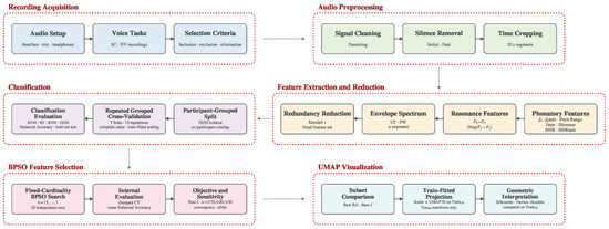
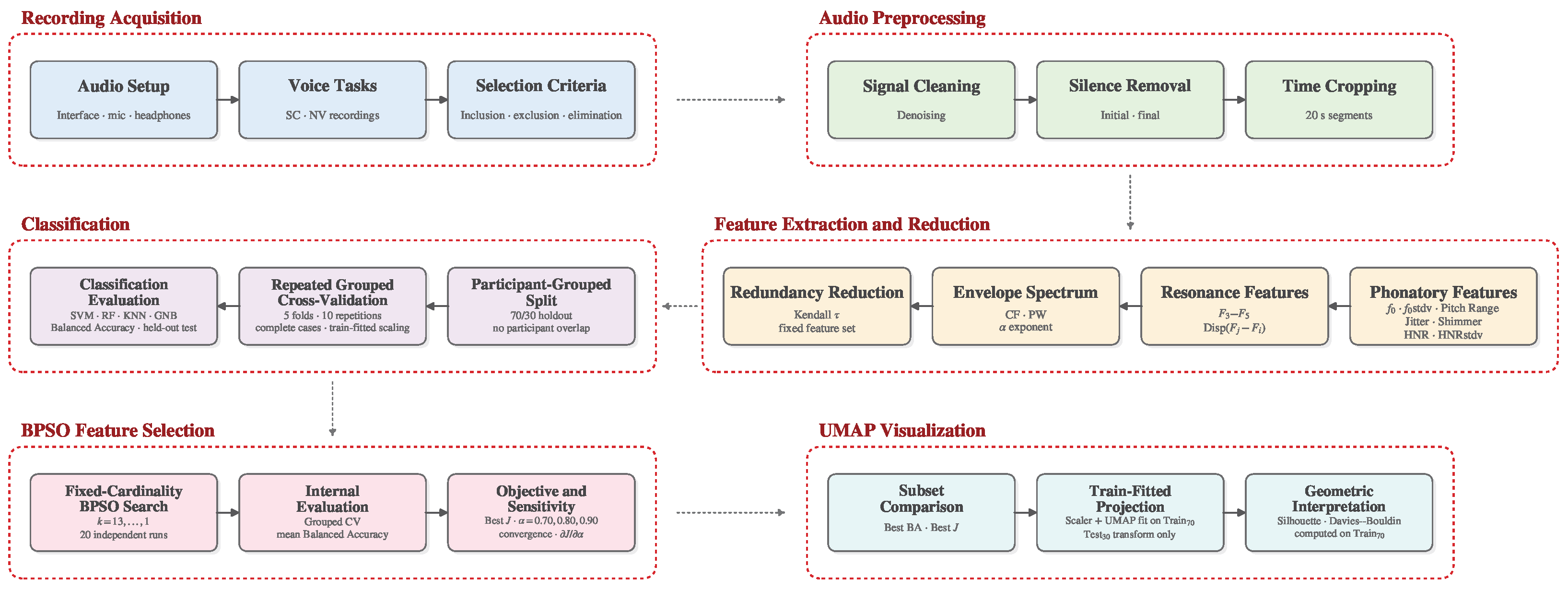
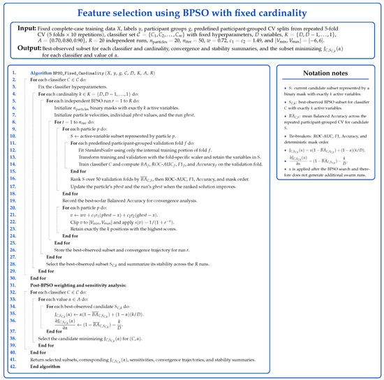
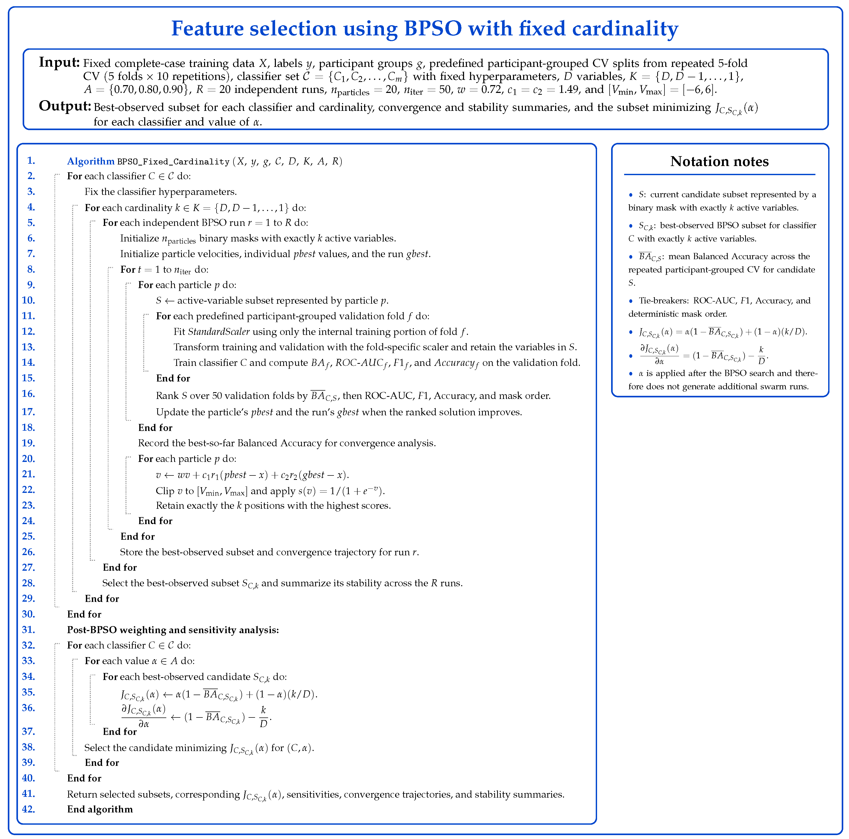
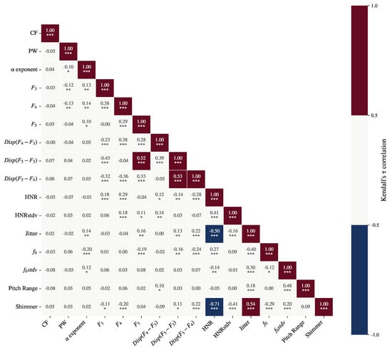
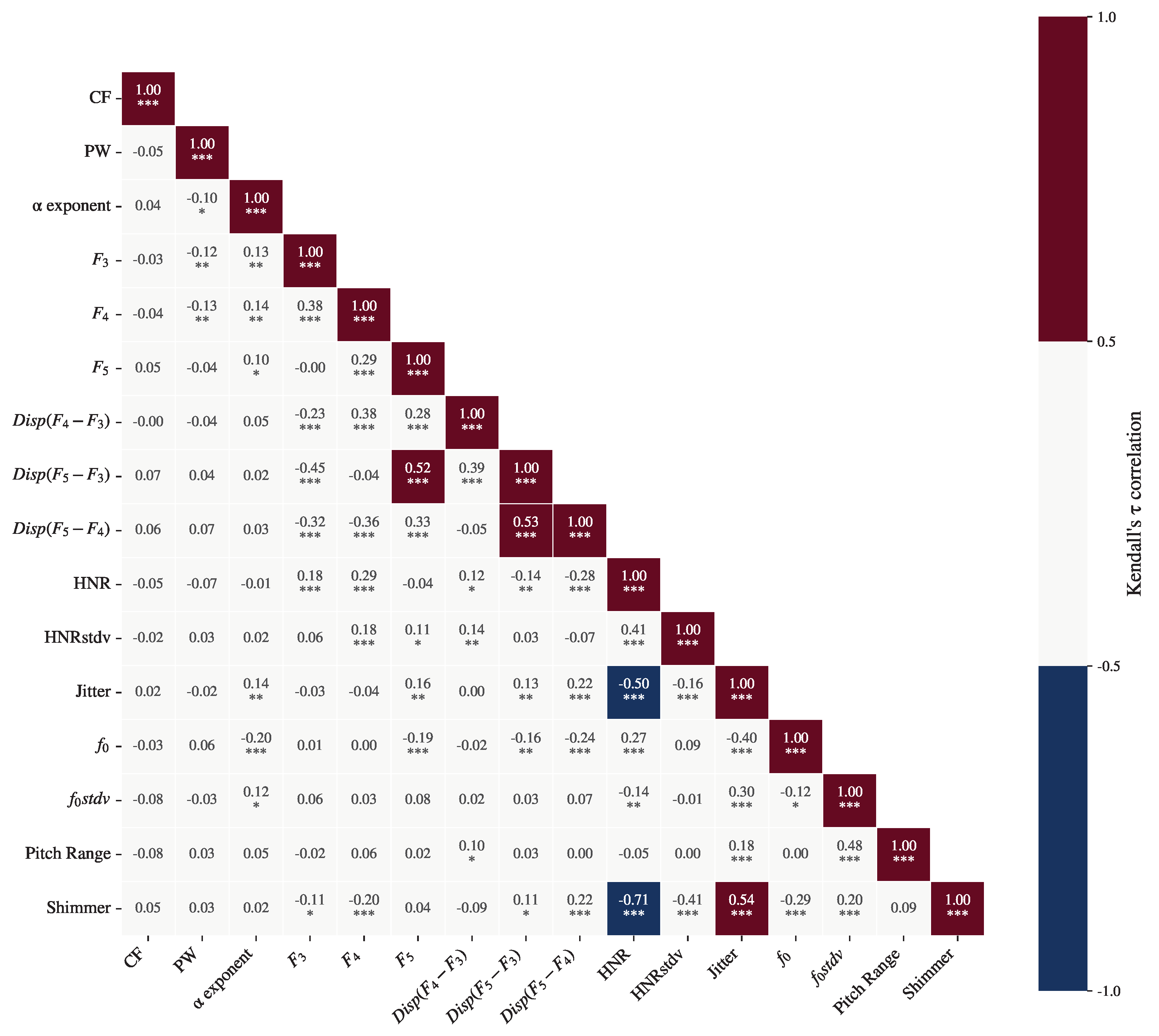
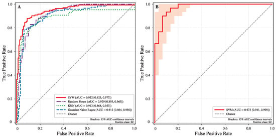
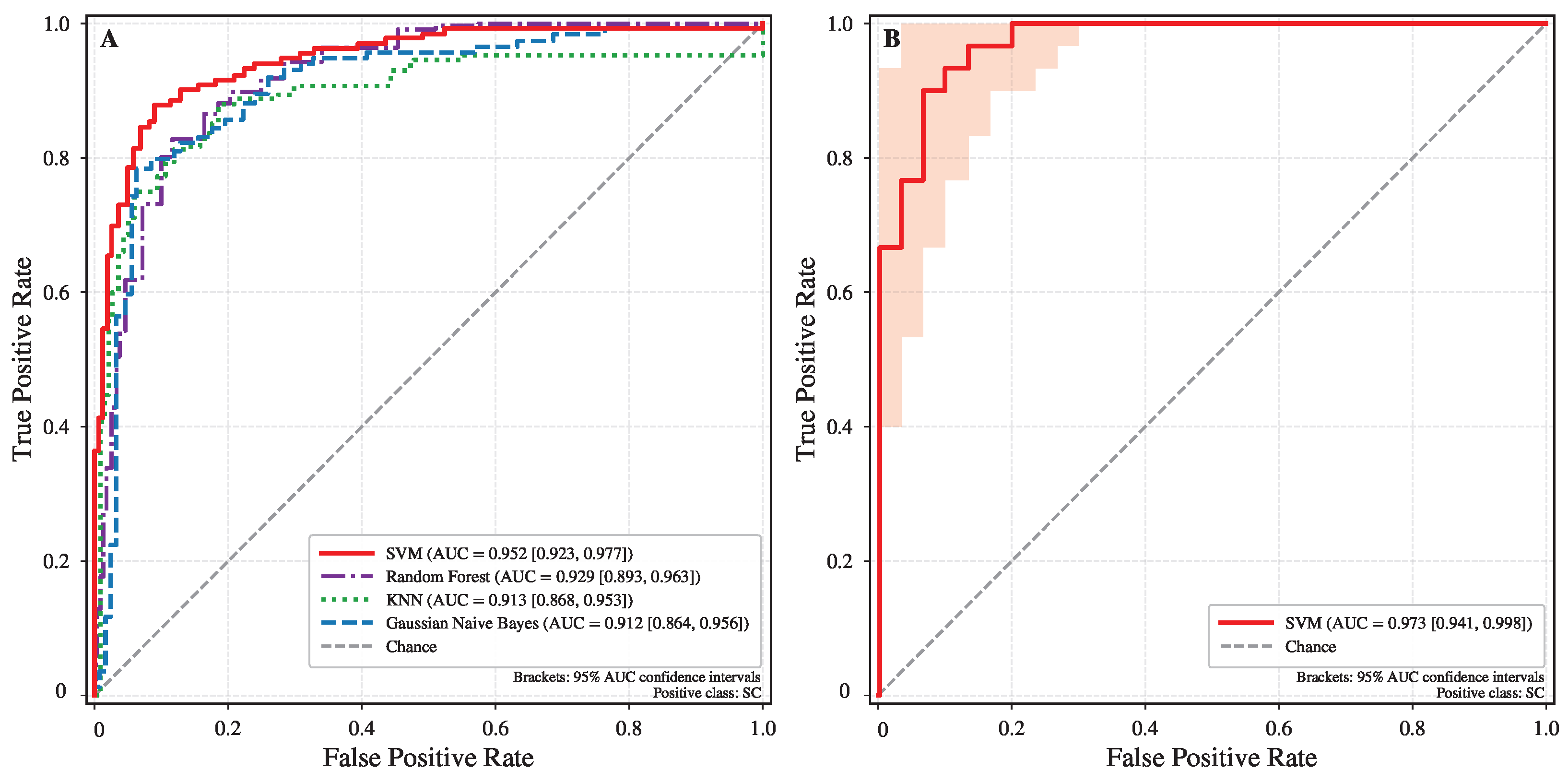
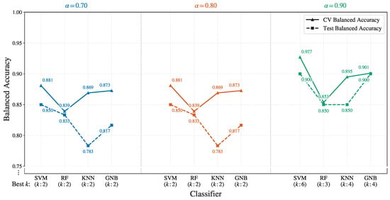
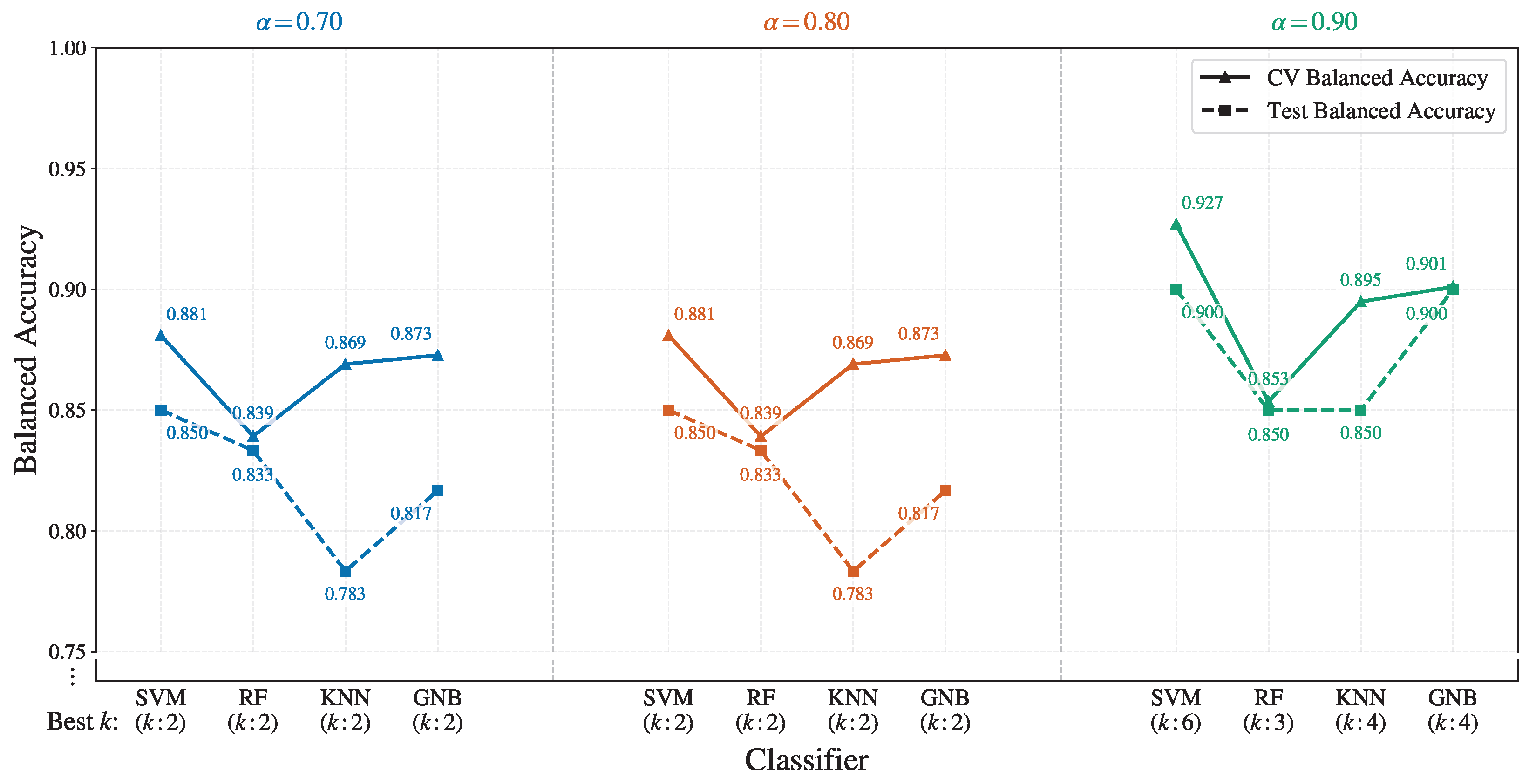
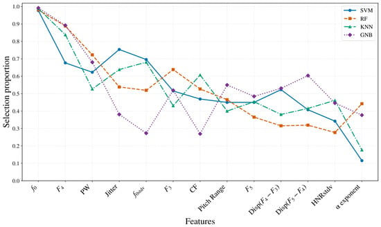
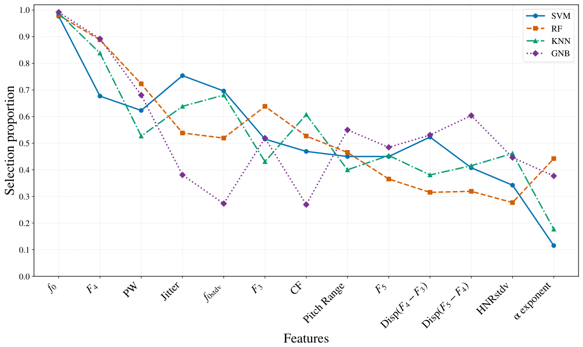
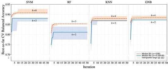
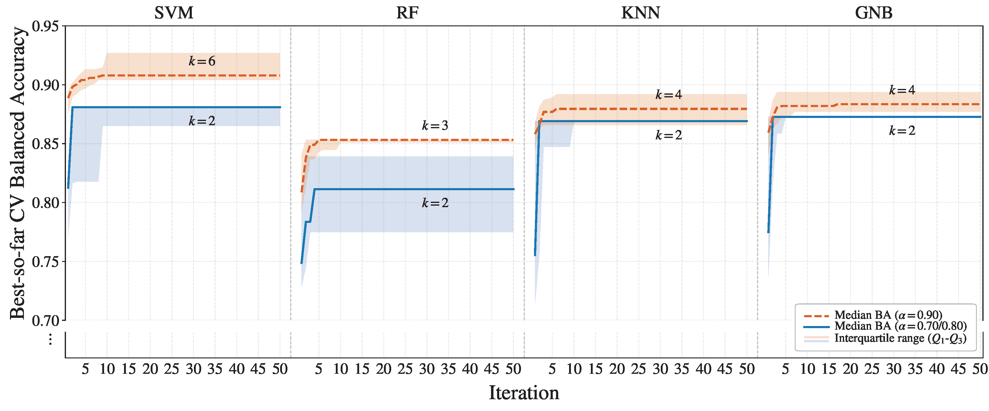
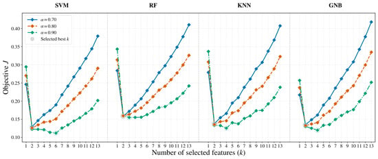
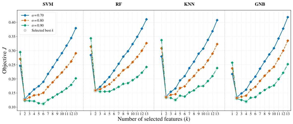
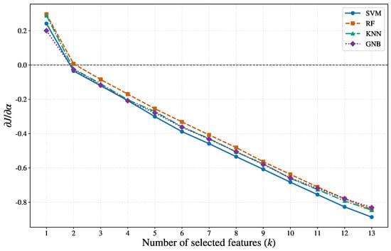
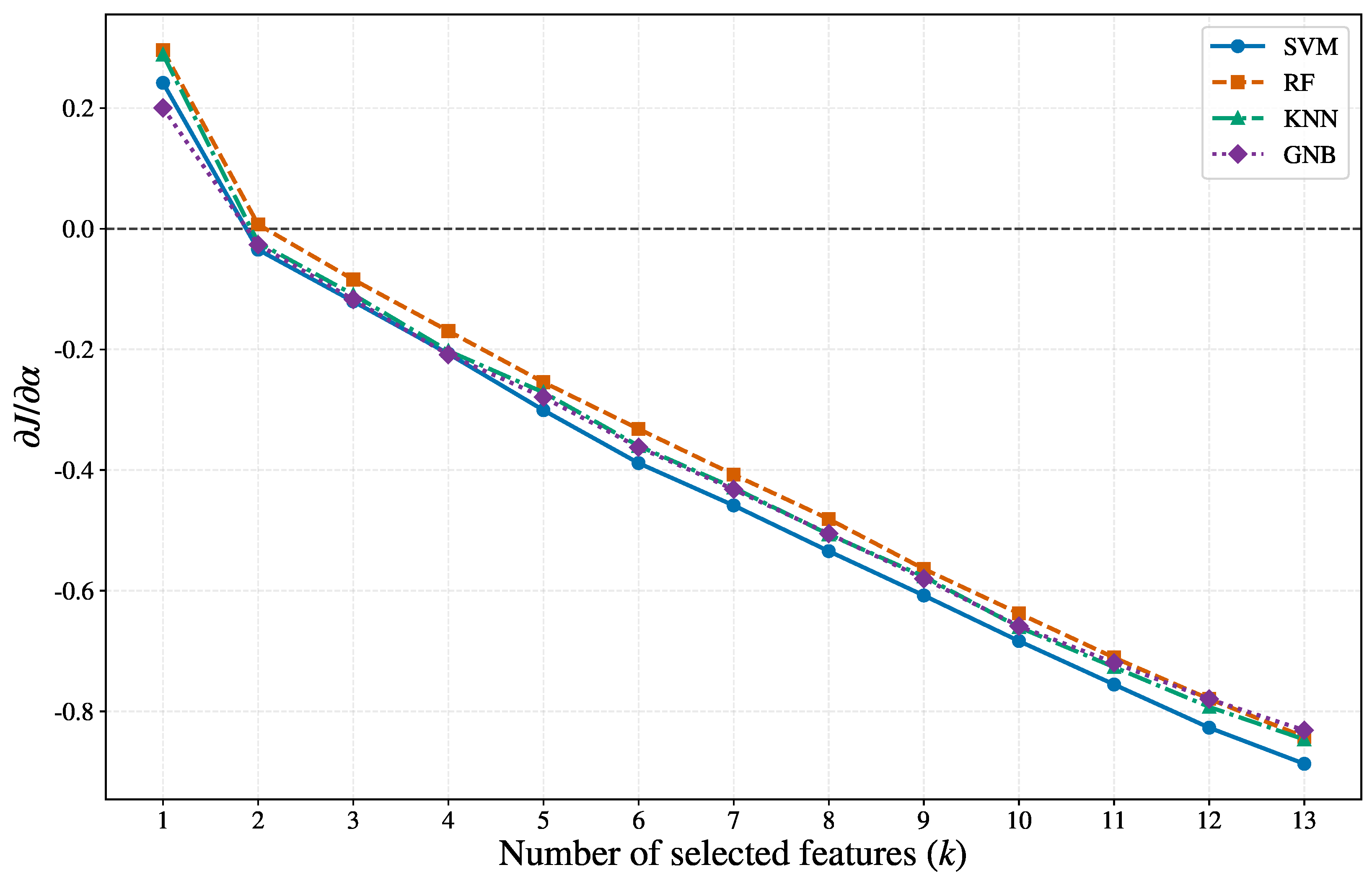
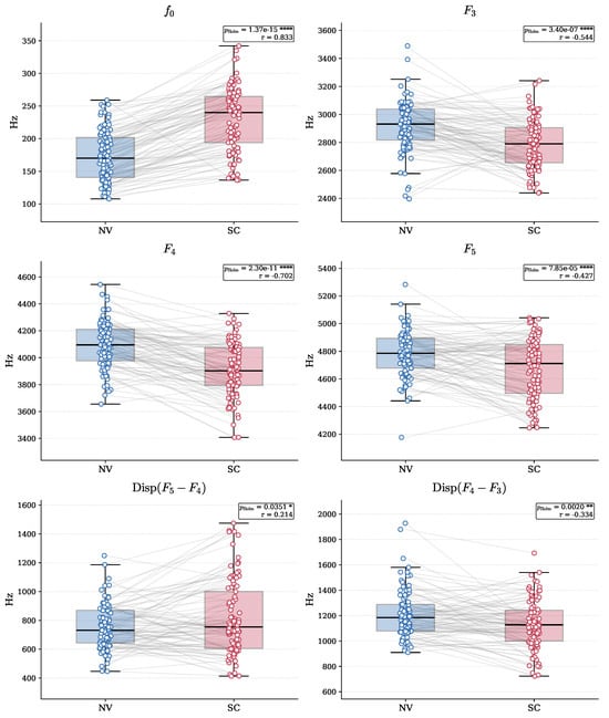
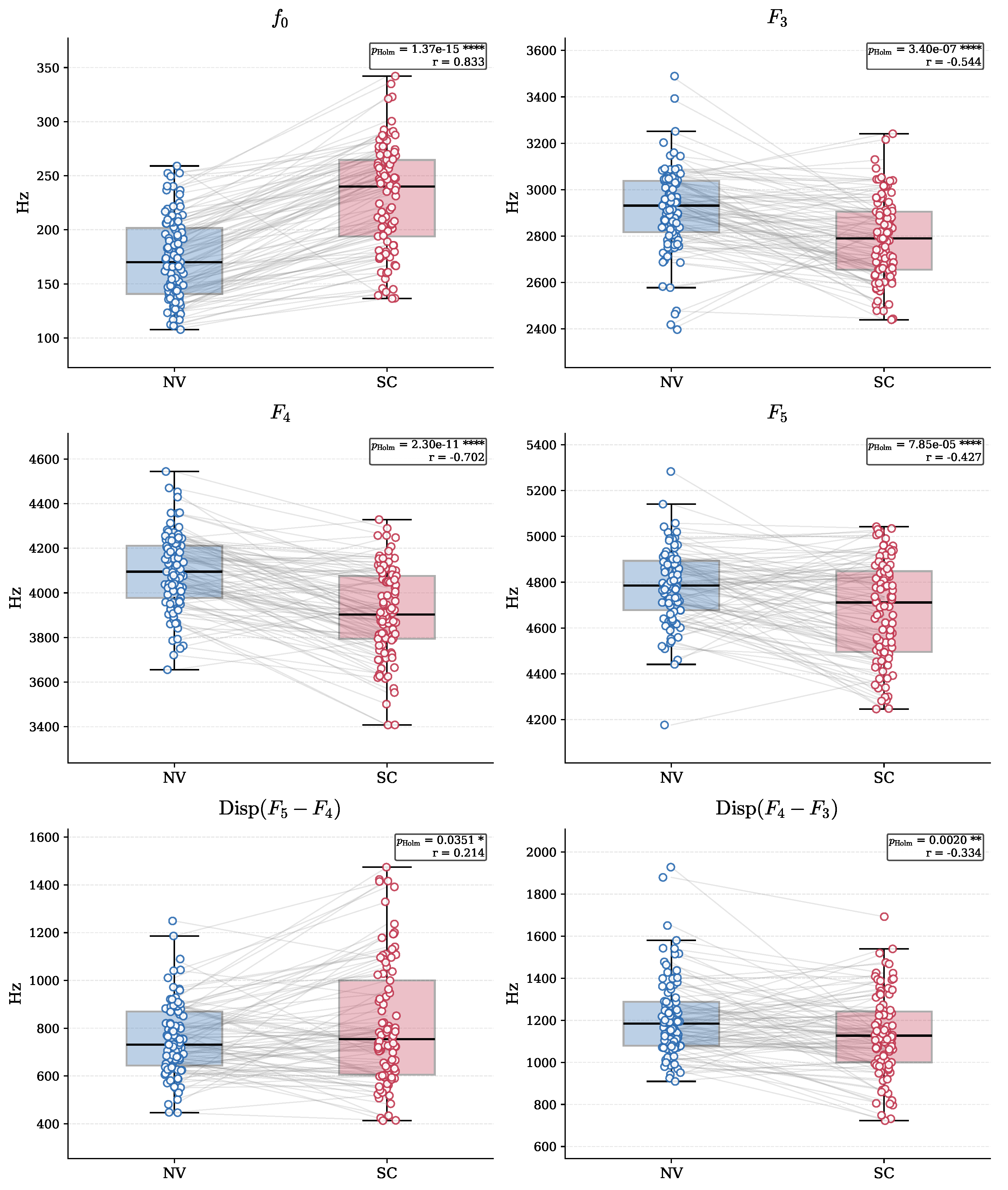
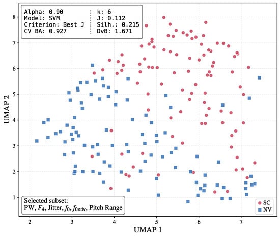
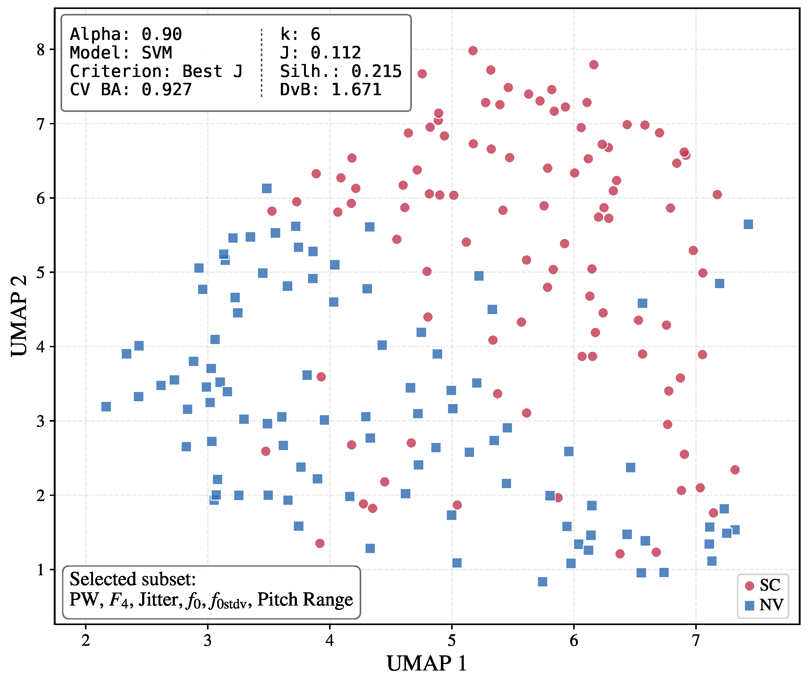
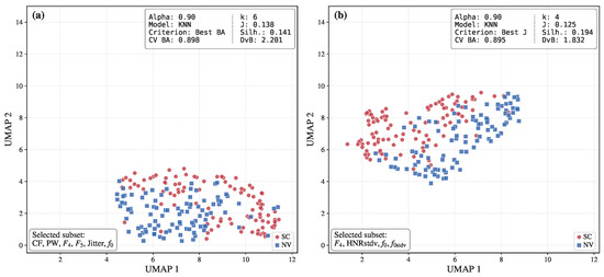
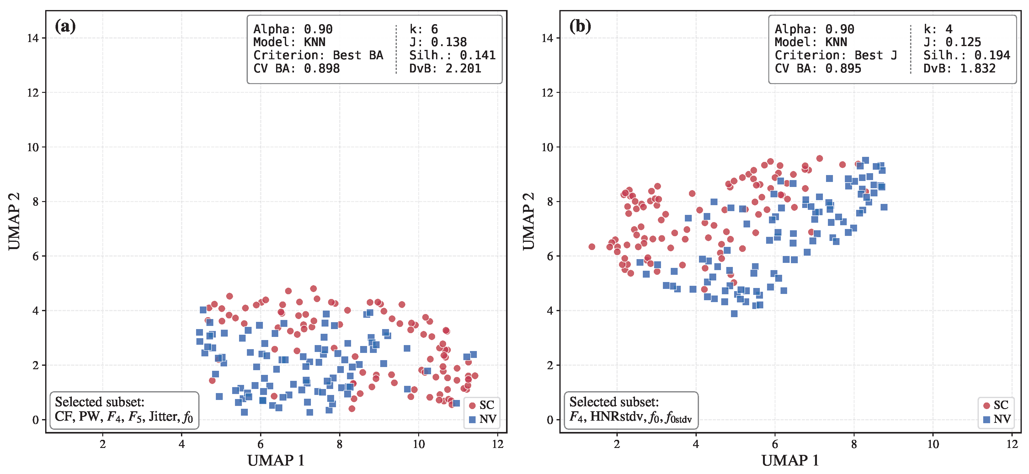

Disclaimer/Publisher’s Note: The statements, opinions and data contained in all publications are solely those of the individual author(s) and contributor(s) and not of MDPI and/or the editor(s). MDPI and/or the editor(s) disclaim responsibility for any injury to people or property resulting from any ideas, methods, instructions or products referred to in the content. |
© 2026 by the authors. Licensee MDPI, Basel, Switzerland. This article is an open access article distributed under the terms and conditions of the Creative Commons Attribution (CC BY) license.