Author Contributions
Conceptualization, S.C., T.L. and Z.J.; methodology, S.C., T.L., X.L. (Xing Li) and C.S.; software, C.S., X.L. (Xin Li) and L.L.; validation, C.W., X.L. (Xin Li) and L.L.; formal analysis, X.L. (Xing Li), X.L. (Xin Li) and C.S.; investigation, S.C., C.W. and L.L.; resources, T.L., X.L. (Xing Li) and Z.J.; data curation, C.S., C.W. and X.L. (Xin Li); writing—original draft preparation, S.C., C.S. and C.W.; writing—review and editing, T.L., X.L. (Xing Li) and Z.J.; visualization, C.S., L.L. and X.L. (Xin Li); supervision, Z.J. and T.L.; project administration, Z.J. and S.C.; funding acquisition, Z.J. and T.L. All authors have read and agreed to the published version of the manuscript.
Figure 1.
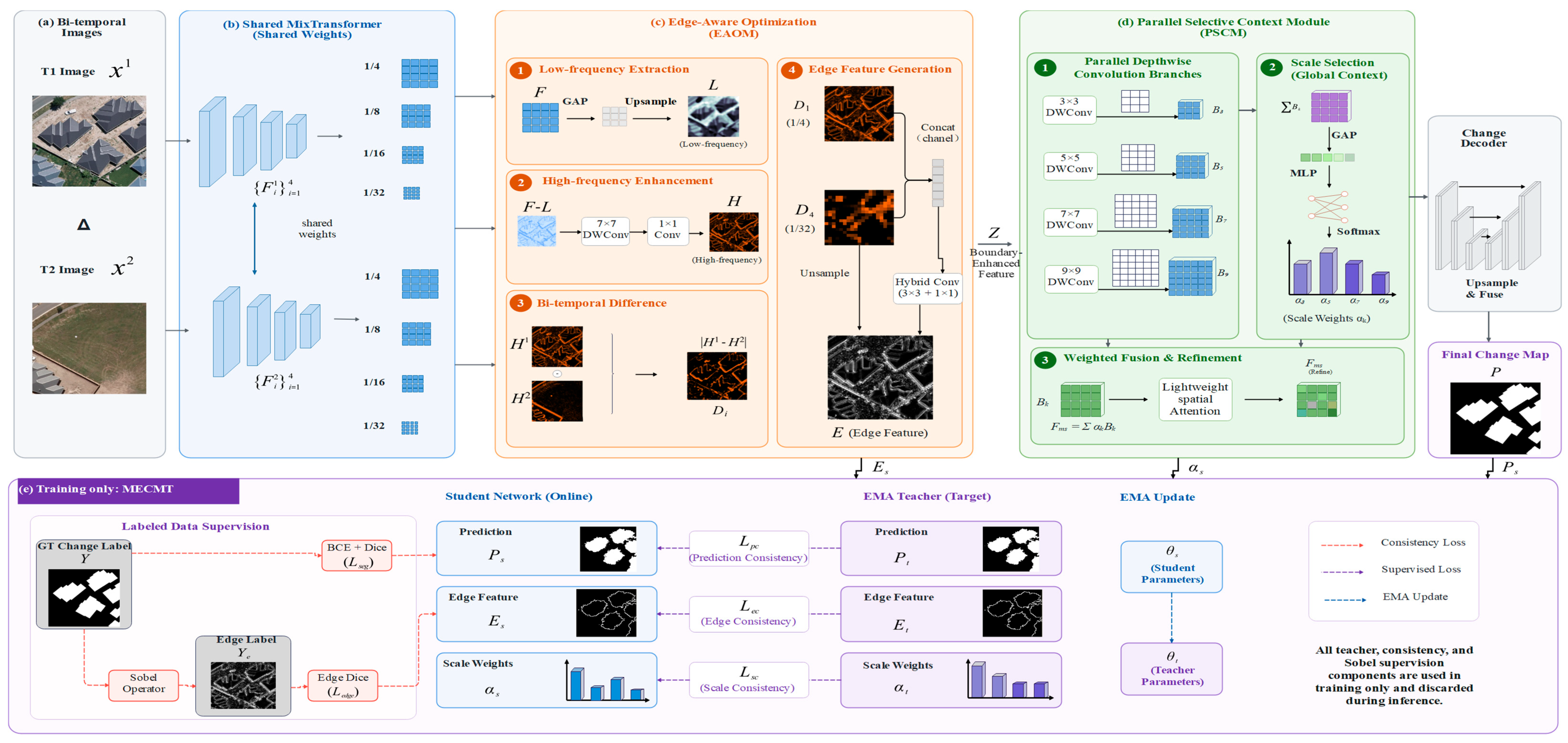
Overall framework of BSCNet. The figure illustrates the data flow and module interactions. (a) Input: Bi-temporal image pairs (T1 and T2) enter a shared MixTransformer encoder. (b) Feature Extraction: The encoder outputs multi-level features. (c) EAOM: A boundary-aware difference representation is constructed and residually modulated. (d) PSCM: Scene-dependent multi-scale context aggregation is performed. (e) MECMT: Prediction-, edge-, and scale-level consistency is imposed between the student and EMA teacher. Arrow colors: Solid black arrows indicate forward data flow; red dashed arrows indicate consistency loss for the student network; purple dashed arrows indicate supervised loss; blue dashed arrows indicate EMA update for the teacher parameters. The “Training only: MECMT” box denotes the semi-supervised training phase, in which all teacher, consistency, and supervised components are used; they are discarded during inference.
Figure 1.
Overall framework of BSCNet. The figure illustrates the data flow and module interactions. (a) Input: Bi-temporal image pairs (T1 and T2) enter a shared MixTransformer encoder. (b) Feature Extraction: The encoder outputs multi-level features. (c) EAOM: A boundary-aware difference representation is constructed and residually modulated. (d) PSCM: Scene-dependent multi-scale context aggregation is performed. (e) MECMT: Prediction-, edge-, and scale-level consistency is imposed between the student and EMA teacher. Arrow colors: Solid black arrows indicate forward data flow; red dashed arrows indicate consistency loss for the student network; purple dashed arrows indicate supervised loss; blue dashed arrows indicate EMA update for the teacher parameters. The “Training only: MECMT” box denotes the semi-supervised training phase, in which all teacher, consistency, and supervised components are used; they are discarded during inference.
Figure 2.
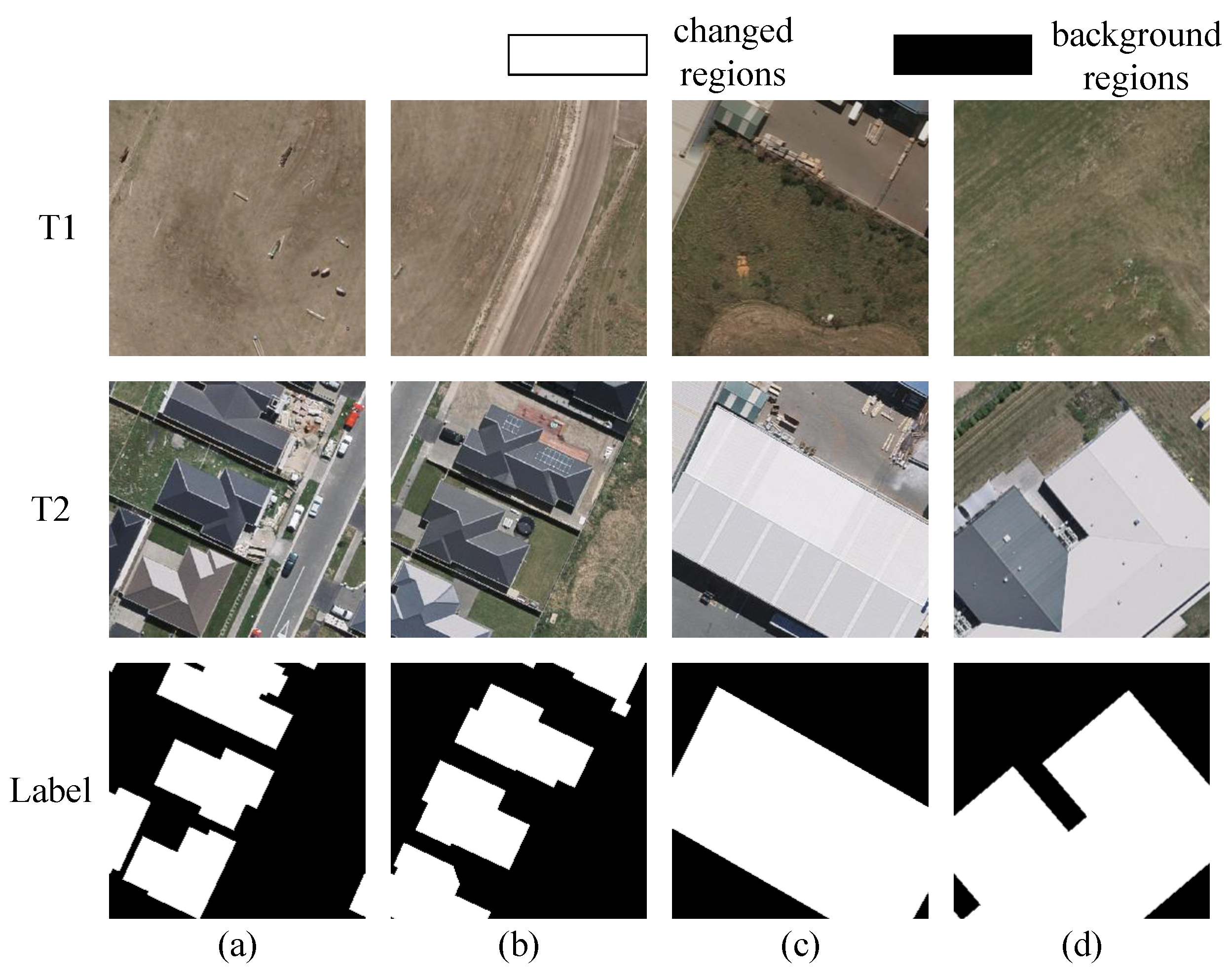
Representative samples from the WHU-CD dataset. (a) Bi-temporal images T1 and T2 for sample 1; (b) Ground-truth change annotation for sample 1; (c) Bi-temporal images T1 and T2 for sample 2; (d) Ground-truth change annotation for sample 2. White pixels denote changed regions, and black pixels denote unchanged regions.
Figure 2.
Representative samples from the WHU-CD dataset. (a) Bi-temporal images T1 and T2 for sample 1; (b) Ground-truth change annotation for sample 1; (c) Bi-temporal images T1 and T2 for sample 2; (d) Ground-truth change annotation for sample 2. White pixels denote changed regions, and black pixels denote unchanged regions.
Figure 3.
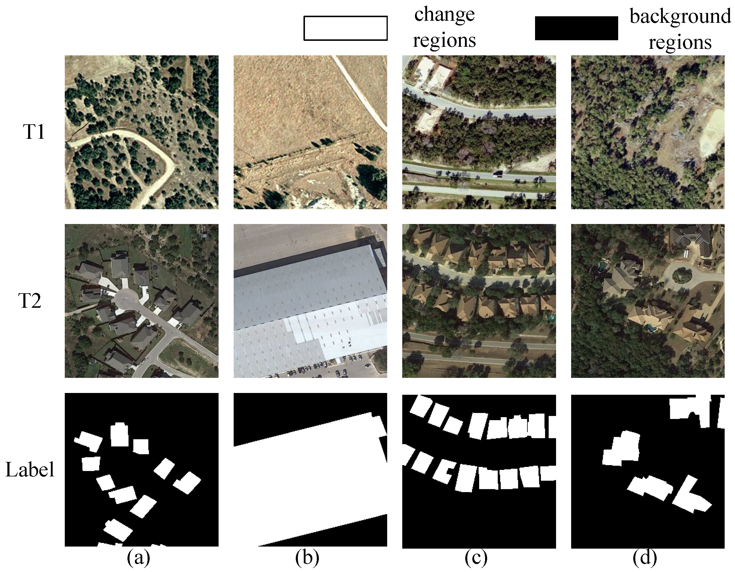
Representative samples from the LEVIR-CD dataset. (a) Bi-temporal images T1 and T2 for sample 1; (b) Ground-truth change annotation for sample 1; (c) Bi-temporal images T1 and T2 for sample 2; (d) Ground-truth change annotation for sample 2. The dataset contains building changes with diverse scales, shapes, orientations, and surrounding environments.
Figure 3.
Representative samples from the LEVIR-CD dataset. (a) Bi-temporal images T1 and T2 for sample 1; (b) Ground-truth change annotation for sample 1; (c) Bi-temporal images T1 and T2 for sample 2; (d) Ground-truth change annotation for sample 2. The dataset contains building changes with diverse scales, shapes, orientations, and surrounding environments.
Figure 4.
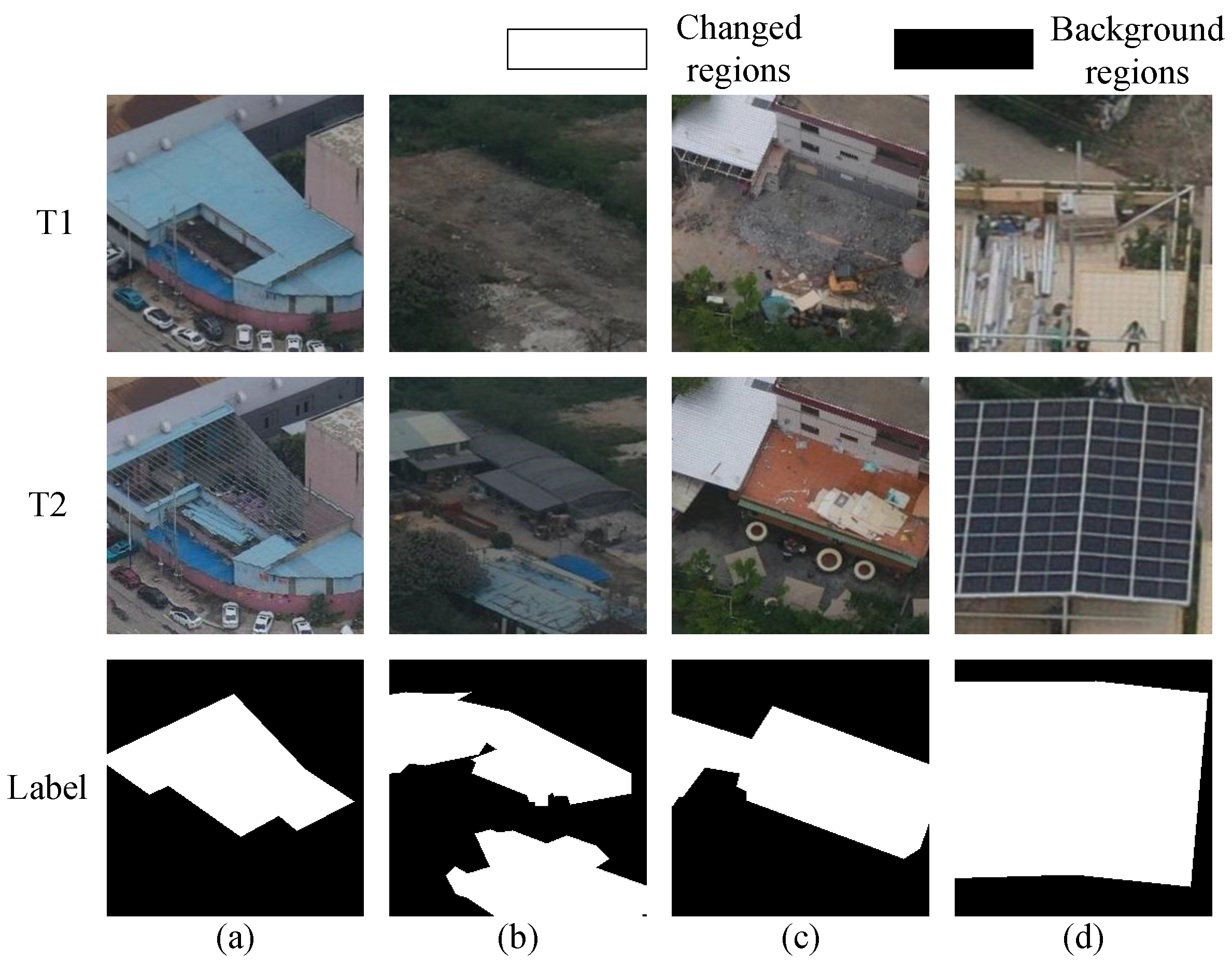
Representative samples from the UAV-CD dataset. (a) Bi-temporal UAV images T1 and T2 for sample 1; (b) Ground-truth change annotation for sample 1; (c) Bi-temporal UAV images T1 and T2 for sample 2; (d) Ground-truth change annotation for sample 2. White pixels denote changed regions, and black pixels denote unchanged regions.
Figure 4.
Representative samples from the UAV-CD dataset. (a) Bi-temporal UAV images T1 and T2 for sample 1; (b) Ground-truth change annotation for sample 1; (c) Bi-temporal UAV images T1 and T2 for sample 2; (d) Ground-truth change annotation for sample 2. White pixels denote changed regions, and black pixels denote unchanged regions.
Figure 5.
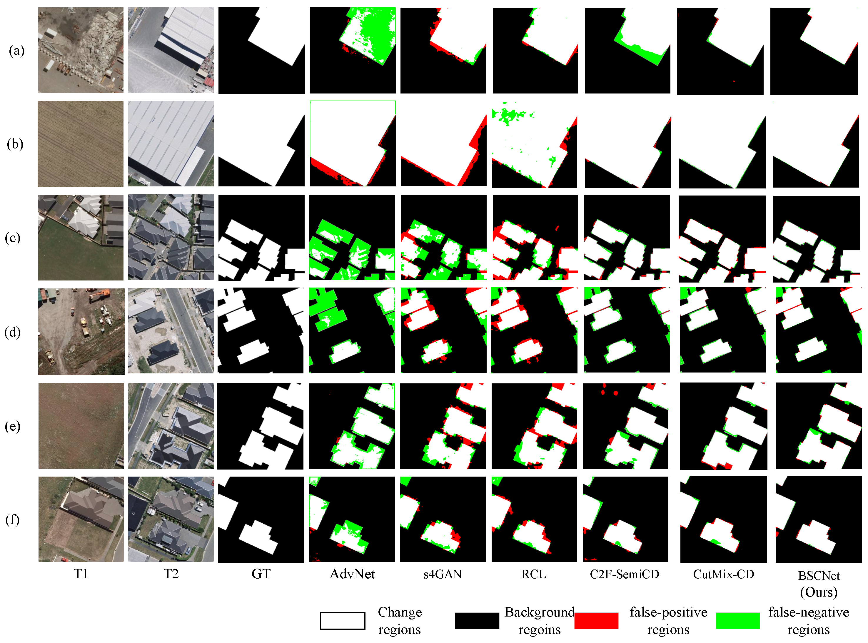
Qualitative comparison on the WHU-CD test set under the 5% labeled-data setting. (a–f) Six representative UAV-CD samples. White and black represent correctly classified change and background regions, while red and green represent false-positive and false-negative regions, respectively.
Figure 5.
Qualitative comparison on the WHU-CD test set under the 5% labeled-data setting. (a–f) Six representative UAV-CD samples. White and black represent correctly classified change and background regions, while red and green represent false-positive and false-negative regions, respectively.
Figure 6.
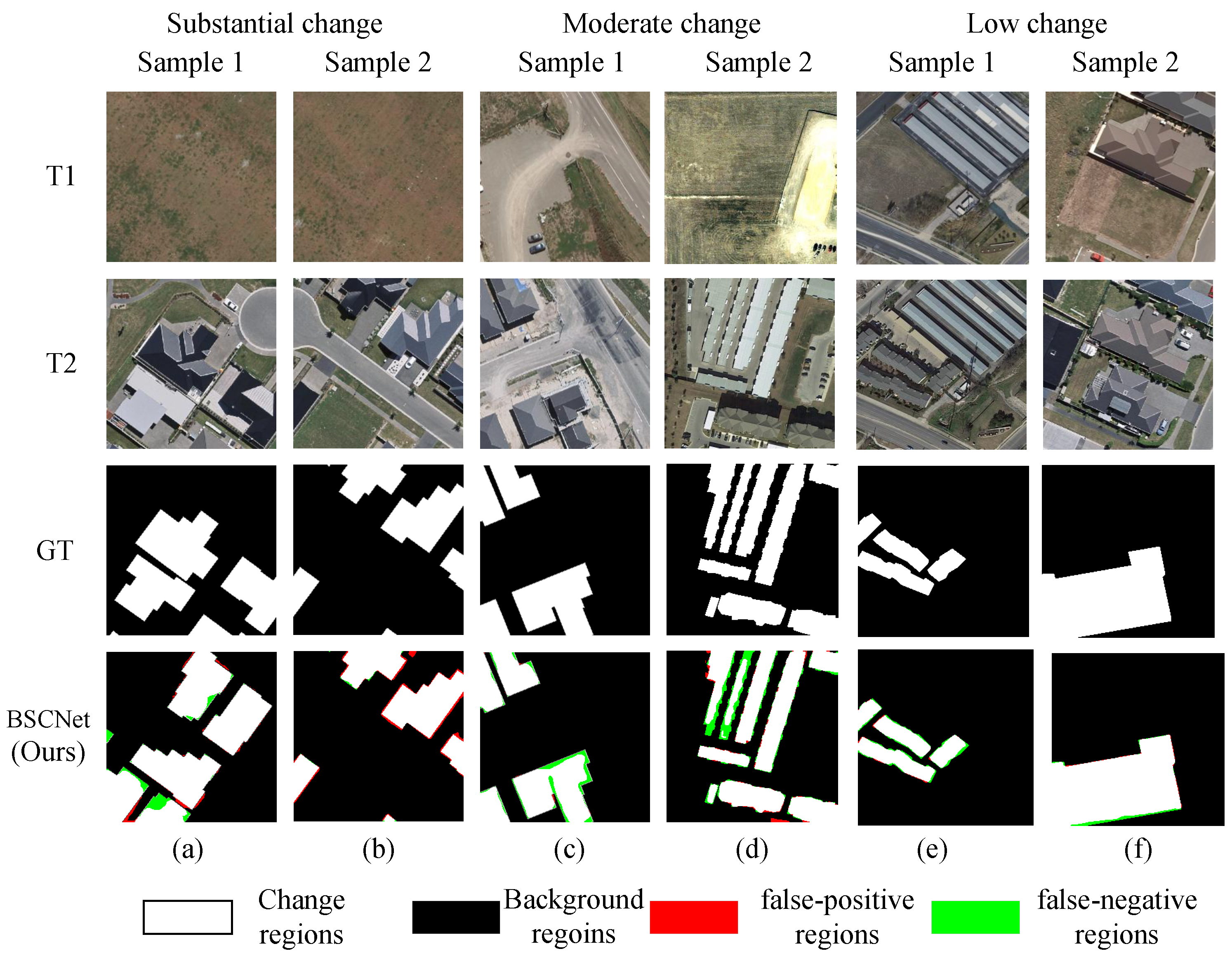
Qualitative results of BSCNet on WHU-CD samples with substantial, moderate, and low bi-temporal changes. (a) Substantial change sample 1; (b) Substantial change sample 2; (c) Moderate change sample 1; (d) Moderate change sample 2; (e) Low change sample 1; (f) Low change sample 2. The rows correspond to T1, T2, ground truth, and the BSCNet prediction. White and black denote correctly classified changed and background regions, respectively, whereas red and green denote false-positive and false-negative regions.
Figure 6.
Qualitative results of BSCNet on WHU-CD samples with substantial, moderate, and low bi-temporal changes. (a) Substantial change sample 1; (b) Substantial change sample 2; (c) Moderate change sample 1; (d) Moderate change sample 2; (e) Low change sample 1; (f) Low change sample 2. The rows correspond to T1, T2, ground truth, and the BSCNet prediction. White and black denote correctly classified changed and background regions, respectively, whereas red and green denote false-positive and false-negative regions.
Figure 7.
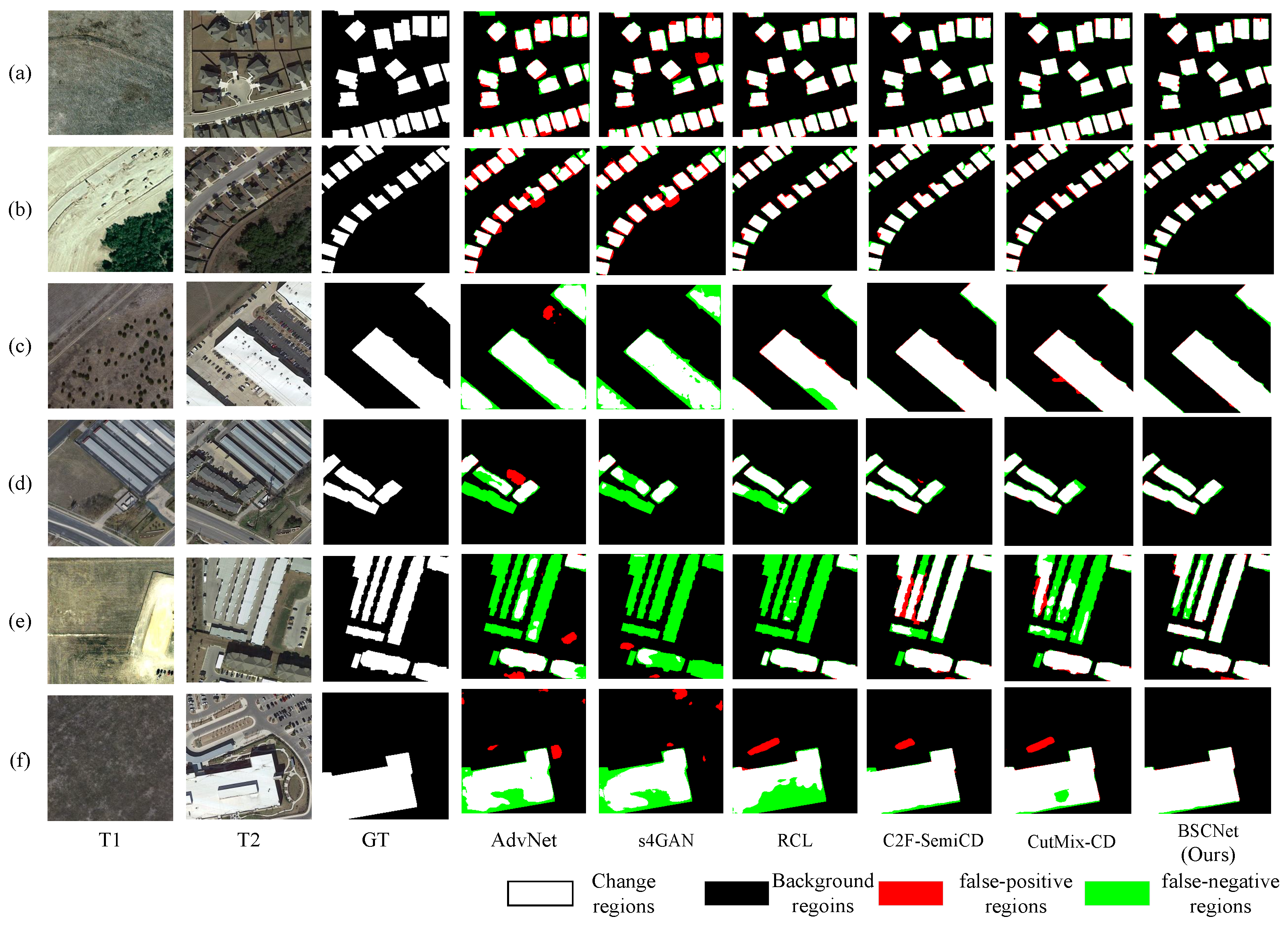
Qualitative comparison on the LEVIR-CD test set under the 10% labeled-data setting. (a–f) Six representative samples. Red and green indicate false-positive and false-negative regions, respectively.
Figure 7.
Qualitative comparison on the LEVIR-CD test set under the 10% labeled-data setting. (a–f) Six representative samples. Red and green indicate false-positive and false-negative regions, respectively.
Figure 8.
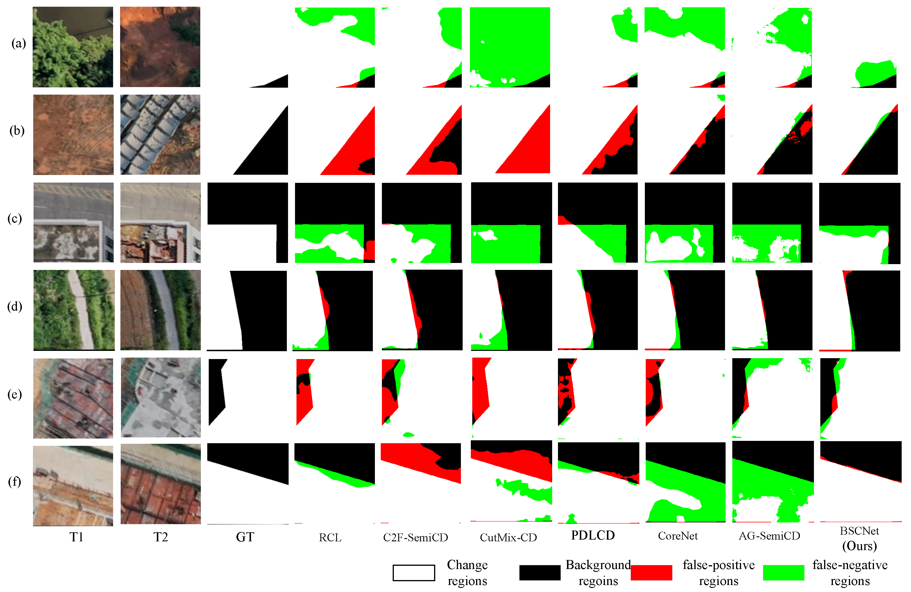
Qualitative comparison on UAV-CD using the same six test samples for all methods. (a–f) Six representative UAV-CD samples. The first three columns show the two temporal images and ground truth, whereas the remaining columns show the prediction results of RCL, C2F-SemiCD, CutMix-CD, PDLCD, CoreNet, AG-SemiCD, and BSCNet. White and black denote correctly classified changed and background regions, respectively, whereas red and green denote false-positive and false-negative regions.
Figure 8.
Qualitative comparison on UAV-CD using the same six test samples for all methods. (a–f) Six representative UAV-CD samples. The first three columns show the two temporal images and ground truth, whereas the remaining columns show the prediction results of RCL, C2F-SemiCD, CutMix-CD, PDLCD, CoreNet, AG-SemiCD, and BSCNet. White and black denote correctly classified changed and background regions, respectively, whereas red and green denote false-positive and false-negative regions.
Figure 9.
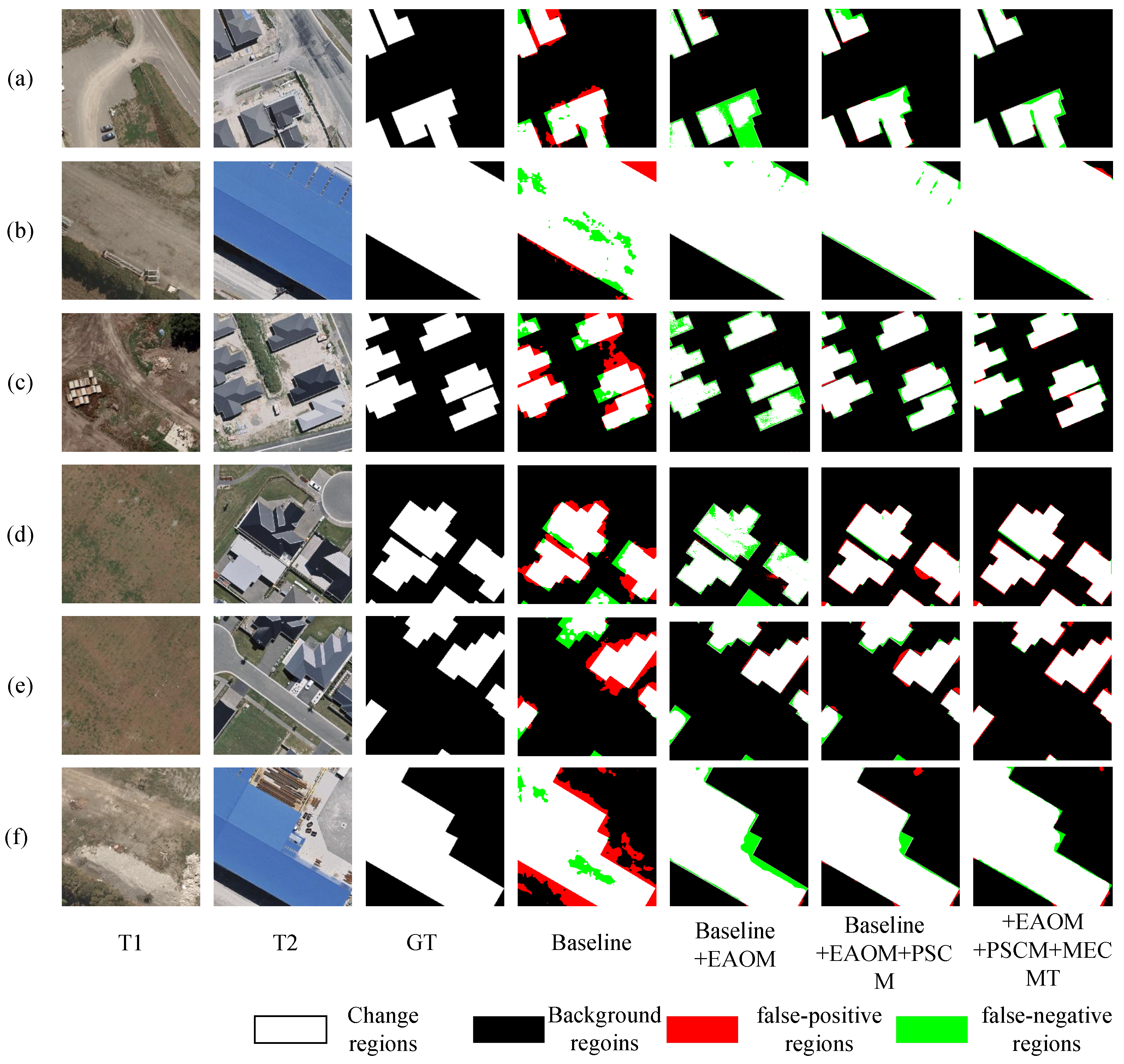
Qualitative ablation results on the WHU-CD test set under the 5% labeled-data setting. (a–f) Six representative samples. Rows correspond to the prediction results of different model configurations (Baseline, +EAOM, +EAOM+PSCM, +EAOM+PSCM+MECMT).
Figure 9.
Qualitative ablation results on the WHU-CD test set under the 5% labeled-data setting. (a–f) Six representative samples. Rows correspond to the prediction results of different model configurations (Baseline, +EAOM, +EAOM+PSCM, +EAOM+PSCM+MECMT).
Figure 10.
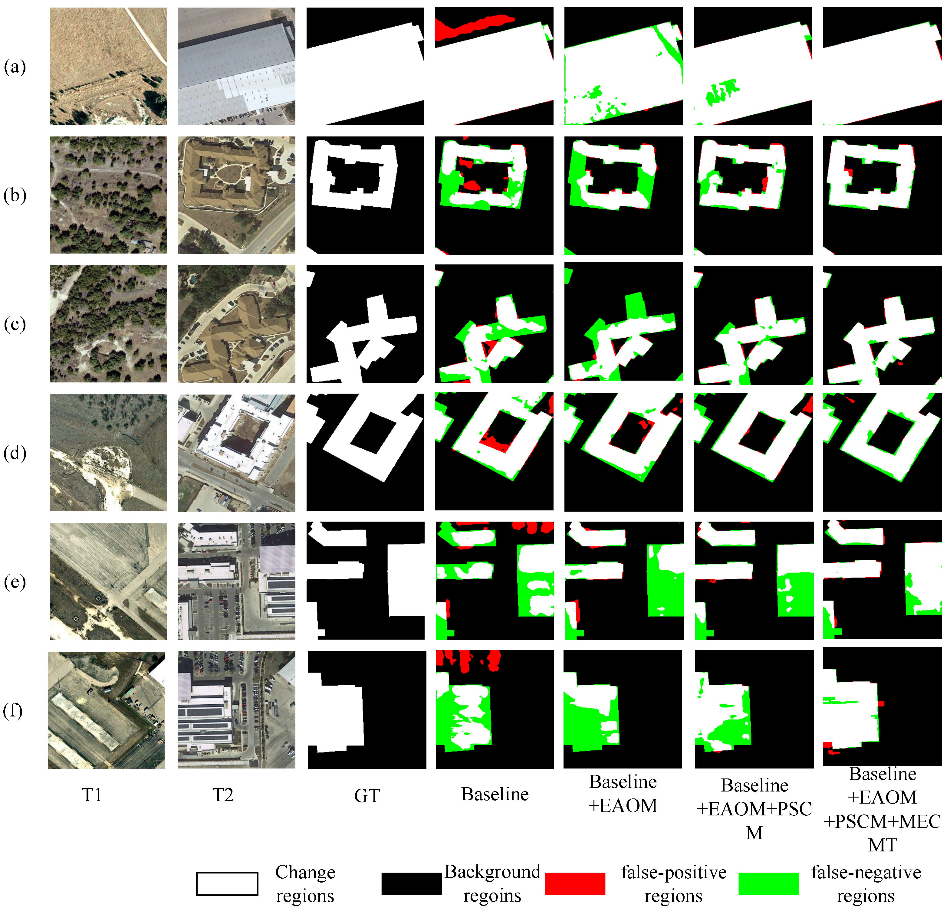
Qualitative ablation results on the LEVIR-CD test set under the 5% labeled-data setting. (a–f) Six representative samples. Rows correspond to the prediction results of different model configurations (Baseline, +EAOM, +EAOM+PSCM, +EAOM+PSCM+MECMT).
Figure 10.
Qualitative ablation results on the LEVIR-CD test set under the 5% labeled-data setting. (a–f) Six representative samples. Rows correspond to the prediction results of different model configurations (Baseline, +EAOM, +EAOM+PSCM, +EAOM+PSCM+MECMT).
Table 1.
Numbers of labeled, unlabeled, validation, and testing samples under different annotation ratios.
Table 1.
Numbers of labeled, unlabeled, validation, and testing samples under different annotation ratios.
| Dataset | Label Ratio | Labeled Train | Unlabeled Train | Validation | Test |
|---|
| WHU-CD | 5% | 304 | 5792 | 762 | 762 |
| 10% | 609 | 5487 | 762 | 762 |
| 20% | 1219 | 4877 | 762 | 762 |
| LEVIR-CD | 5% | 356 | 6764 | 1024 | 2048 |
| 10% | 712 | 6408 | 1024 | 2048 |
| 20% | 1424 | 5696 | 1024 | 2048 |
Table 2.
Main training parameters of BSCNet.
Table 2.
Main training parameters of BSCNet.
| Parameter | Value |
|---|
| Optimizer | Adam |
| Initial learning rate | |
| Weight decay | |
| Total batch size | 8 (4 labeled + 4 unlabeled) |
| Training epochs | 80 |
| Teacher update | EMA () |
| Pseudo-label threshold | 0.5 |
| Ramp-up duration | 30 epochs |
| Overall consistency weight | Exponential ramp-up () |
| Consistency-term weights | for |
| Evaluation model | Best-validation EMA teacher |
Table 3.
Quantitative comparison on the WHU-CD test set. F1 and IoU are reported in percentages. For RCL, C2F-SemiCD, CutMix-CD, and BSCNet, values are reported as mean ± standard deviation over five independent runs; the remaining methods are shown as literature-reported point estimates.
Table 3.
Quantitative comparison on the WHU-CD test set. F1 and IoU are reported in percentages. For RCL, C2F-SemiCD, CutMix-CD, and BSCNet, values are reported as mean ± standard deviation over five independent runs; the remaining methods are shown as literature-reported point estimates.
| Method | 5% Labels | 10% Labels | 20% Labels |
|---|
| F1 | IoU | F1 | IoU | F1 | IoU |
|---|
| RCL [35] | 77.69 ± 0.52 | 63.52 ± 0.69 | 83.61 ± 0.39 | 71.84 ± 0.58 | 86.08 ± 0.31 | 75.56 ± 0.48 |
| C2F-SemiCD [36] | 84.55 ± 0.35 | 73.24 ± 0.52 | 88.79 ± 0.26 | 79.84 ± 0.42 | 90.16 ± 0.21 | 82.08 ± 0.35 |
| CutMix-CD [37] | 87.56 ± 0.30 | 77.87 ± 0.47 | 88.71 ± 0.25 | 79.71 ± 0.40 | 88.83 ± 0.22 | 79.90 ± 0.36 |
| RISL [38] | 89.80 | 81.48 | 90.46 | 82.59 | 91.14 | 83.72 |
| PDLCD [39] | 91.14 | 83.72 | 92.82 | 86.60 | 93.65 | 88.05 |
| AdaSemiCD [41] | 80.81 | 67.80 | 82.90 | 70.80 | 85.32 | 74.40 |
| BRT [70] | 90.17 | 82.10 | 91.01 | 83.50 | 91.54 | 84.40 |
| SemiCD-VL [52] | 89.99 | 81.80 | 90.83 | 83.20 | 91.77 | 84.80 |
| CoreNet [47] | 91.48 | 84.30 | 92.24 | 85.60 | 92.88 | 86.70 |
| AG-SemiCD [48] | 91.66 | 84.60 | 92.47 | 86.00 | 93.11 | 87.10 |
| BSCNet | 88.57 ± 0.28 | 79.49 ± 0.45 | 89.53 ± 0.23 | 81.05 ± 0.38 | 90.47 ± 0.19 | 82.59 ± 0.32 |
Table 4.
Quantitative comparison on the LEVIR-CD test set. F1 and IoU are reported in percentages. For RCL, C2F-SemiCD, CutMix-CD, and BSCNet, values are reported as mean ± standard deviation over five independent runs; the remaining methods are shown as literature-reported point estimates.
Table 4.
Quantitative comparison on the LEVIR-CD test set. F1 and IoU are reported in percentages. For RCL, C2F-SemiCD, CutMix-CD, and BSCNet, values are reported as mean ± standard deviation over five independent runs; the remaining methods are shown as literature-reported point estimates.
| Method | 5% Labels | 10% Labels | 20% Labels |
|---|
| F1 | IoU | F1 | IoU | F1 | IoU |
|---|
| RCL [35] | 83.78 ± 0.41 | 72.09 ± 0.61 | 85.87 ± 0.34 | 75.23 ± 0.52 | 86.77 ± 0.29 | 76.64 ± 0.45 |
| C2F-SemiCD [36] | 88.44 ± 0.27 | 79.28 ± 0.44 | 89.67 ± 0.23 | 81.28 ± 0.38 | 90.72 ± 0.20 | 83.02 ± 0.33 |
| CutMix-CD [37] | 87.74 ± 0.26 | 78.15 ± 0.42 | 88.91 ± 0.23 | 80.03 ± 0.37 | 89.53 ± 0.20 | 81.05 ± 0.32 |
| RISL [38] | 90.06 | 81.92 | 90.45 | 82.56 | 90.51 | 82.67 |
| PDLCD [39] | 90.89 | 83.30 | 91.16 | 83.75 | 91.48 | 84.30 |
| AdaSemiCD [41] | 87.45 | 77.70 | 88.52 | 79.40 | 89.07 | 80.30 |
| BRT [70] | 90.71 | 83.00 | 91.19 | 83.80 | 91.60 | 84.50 |
| SemiCD-VL [52] | 90.05 | 81.90 | 90.47 | 82.60 | 90.53 | 82.70 |
| CoreNet [47] | 91.30 | 84.00 | 91.66 | 84.60 | 91.95 | 85.10 |
| AG-SemiCD [48] | 91.60 | 84.50 | 91.95 | 85.10 | 92.24 | 85.60 |
| BSCNet | 88.88 ± 0.24 | 79.98 ± 0.39 | 89.92 ± 0.20 | 81.68 ± 0.33 | 90.90 ± 0.17 | 83.31 ± 0.29 |
Table 5.
Semi-supervised generalization results on UAV-CD under different labeled-data ratios. F1 and IoU are reported in percentages. Results are reported under the same 5%, 10%, and 20% labeled-data settings used in the core evaluation.
Table 5.
Semi-supervised generalization results on UAV-CD under different labeled-data ratios. F1 and IoU are reported in percentages. Results are reported under the same 5%, 10%, and 20% labeled-data settings used in the core evaluation.
| Method | 5% Labels | 10% Labels | 20% Labels |
|---|
| F1 | IoU | F1 | IoU | F1 | IoU |
|---|
| RCL [35] | 59.94 | 42.80 | 62.40 | 45.35 | 64.50 | 47.60 |
| C2F-SemiCD [36] | 65.73 | 48.95 | 67.64 | 51.10 | 69.45 | 53.20 |
| CutMix-CD [37] | 66.40 | 49.70 | 68.29 | 51.85 | 70.21 | 54.10 |
| BSCNet | 68.07 | 51.60 | 70.00 | 53.85 | 71.71 | 55.90 |
Table 6.
Progressive ablation results on WHU-CD and LEVIR-CD. EAOM, PSCM, and MECMT denote the Edge-Aware Optimization Module, Parallel Selective Context Module, and Multi-scale Edge-Consistent Mean Teacher framework, respectively. The symbol “✓” indicates that the component is enabled, and “–” indicates that it is disabled.
Table 6.
Progressive ablation results on WHU-CD and LEVIR-CD. EAOM, PSCM, and MECMT denote the Edge-Aware Optimization Module, Parallel Selective Context Module, and Multi-scale Edge-Consistent Mean Teacher framework, respectively. The symbol “✓” indicates that the component is enabled, and “–” indicates that it is disabled.
| Dataset | Label Ratio | EAOM | PSCM | MECMT | F1 | Pre | IoU | Rec |
|---|
| WHU-CD | 5% | – | – | – | 81.44 | 81.04 | 68.69 | 81.83 |
| ✓ | – | – | 84.59 | 82.22 | 73.29 | 87.10 |
| ✓ | ✓ | – | 86.68 | 85.40 | 76.49 | 87.99 |
| ✓ | ✓ | ✓ | 88.57 | 86.08 | 79.49 | 91.22 |
| 10% | – | – | – | 83.64 | 82.73 | 71.89 | 84.58 |
| ✓ | – | – | 86.05 | 83.24 | 75.52 | 89.07 |
| ✓ | ✓ | – | 88.20 | 86.60 | 78.89 | 89.86 |
| ✓ | ✓ | ✓ | 89.53 | 86.86 | 81.05 | 92.38 |
| LEVIR-CD | 5% | – | – | – | 82.80 | 82.33 | 70.64 | 83.27 |
| ✓ | – | – | 85.12 | 83.32 | 74.10 | 87.01 |
| ✓ | ✓ | – | 87.46 | 86.07 | 77.71 | 88.88 |
| ✓ | ✓ | ✓ | 88.88 | 87.62 | 79.98 | 90.17 |
| 10% | – | – | – | 84.63 | 84.32 | 73.35 | 84.94 |
| ✓ | – | – | 87.01 | 85.20 | 77.01 | 88.90 |
| ✓ | ✓ | – | 89.18 | 88.05 | 80.47 | 90.33 |
| ✓ | ✓ | ✓ | 89.92 | 88.27 | 81.68 | 91.62 |
Table 7.
Ablation of the MECMT consistency terms under 5% supervision. PC, EC, and SC denote prediction consistency, edge-feature consistency, and scale-selection consistency, respectively.
Table 7.
Ablation of the MECMT consistency terms under 5% supervision. PC, EC, and SC denote prediction consistency, edge-feature consistency, and scale-selection consistency, respectively.
| Configuration | PC | EC | SC | WHU-CD | LEVIR-CD |
|---|
| F1 | IoU | F1 | IoU |
|---|
| Supervised-only full architecture | – | – | – | 86.68 | 76.49 | 87.46 | 77.71 |
| Prediction-only Mean Teacher | ✓ | – | – | 87.53 | 77.82 | 88.04 | 78.63 |
| PC + edge consistency | ✓ | ✓ | – | 88.06 | 78.67 | 88.42 | 79.25 |
| PC + scale consistency | ✓ | – | ✓ | 87.84 | 78.31 | 88.31 | 79.06 |
| Full MECMT | ✓ | ✓ | ✓ | 88.57 | 79.49 | 88.88 | 79.98 |
Table 8.
Comparison of edge-supervision and edge-modulation designs under 5% supervision.
Table 8.
Comparison of edge-supervision and edge-modulation designs under 5% supervision.
| Variant | WHU-CD | LEVIR-CD |
|---|
| F1 | IoU | F1 | IoU |
|---|
| No edge branch | 86.92 | 76.87 | 87.46 | 77.71 |
| Auxiliary edge supervision only | 87.63 | 77.99 | 88.05 | 78.65 |
| Direct modulation: | 87.24 | 77.36 | 87.81 | 78.27 |
| Residual modulation: | 88.57 | 79.49 | 88.88 | 79.98 |
Table 9.
Comparison of scale-aggregation strategies under 5% supervision.
Table 9.
Comparison of scale-aggregation strategies under 5% supervision.
| Scale Strategy | WHU-CD | LEVIR-CD |
|---|
| F1 | IoU | F1 | IoU |
|---|
| Single branch | 87.55 | 77.86 | 88.13 | 78.78 |
| Single branch | 87.78 | 78.22 | 88.29 | 79.03 |
| Single branch | 87.85 | 78.34 | 88.41 | 79.23 |
| Single branch | 87.69 | 78.08 | 88.24 | 78.96 |
| Uniform average of four branches | 88.08 | 78.70 | 88.55 | 79.45 |
| Learned PSCM weighting | 88.57 | 79.49 | 88.88 | 79.98 |
Table 10.
Sensitivity analysis of the edge- and scale-consistency weights under 5% supervision.
Table 10.
Sensitivity analysis of the edge- and scale-consistency weights under 5% supervision.
| | WHU-CD IoU | LEVIR-CD IoU |
|---|
| 0 | 0 | 77.82 | 78.63 |
| 0.05 | 0.01 | 78.88 | 79.31 |
| 0.10 | 0.005 | 79.31 | 79.82 |
| 0.10 | 0.01 | 79.49 | 79.98 |
| 0.10 | 0.02 | 79.18 | 79.64 |
| 0.20 | 0.01 | 79.22 | 79.71 |
Table 11.
Computational complexity and practical efficiency under the unified bi-temporal input configuration.
Table 11.
Computational complexity and practical efficiency under the unified bi-temporal input configuration.
| Method | FLOPs (G) | Params (M) | Training Time (s/epoch) | Peak Memory (GB) | Inference Latency (ms/pair) |
|---|
| RCL [35] | 73.23 | 46.85 | 198 | 14.3 | 22.6 |
| C2F-SemiCD [36] | 62.10 | 16.17 | 176 | 11.5 | 20.1 |
| CutMix-CD [37] | 72.91 | 46.85 | 205 | 14.7 | 23.0 |
| BSCNet | 45.72 | 47.13 | 184 | 13.2 | 17.8 |



 ,
,