Observer-Based Stabilization of an Incommensurate Fractional-Order Discrete-Time SI Computer Virus Model

Abstract

This paper studies observer-based stabilization of a normalized incommensurate fractional-order discrete-time SI benchmark model for computer-virus propagation. The model is formulated with Caputo-like fractional-difference operators and allows the susceptible and infected compartments to have different memory orders. In contrast with a predictive malware-forecasting model, the proposed system is explicitly treated as a dimensionless benchmark for qualitative analysis and control design. To clarify how the benchmark can be connected to empirical cybersecurity data, the revised formulation includes a calibration and fractional-order selection procedure based on normalized infection telemetry, admissible parameter sets, and loss minimization. The incommensurate orders are therefore interpreted as identifiable modeling parameters, not as arbitrary constants. The plant, observer, and control laws are formulated on the integer update grid, and the memory terms are implemented through the equivalent Volterra-type convolution representation. A nonlinear Luenberger-type observer is proposed under infected-state measurements, which is justified as a detectability-based cyber-monitoring configuration rather than a full observability assumption. The observer gain design, the full-state feedback design, and the observer-based output-feedback design are derived from first-order linearized incommensurate fractional-order models. The resulting criteria are expressed through characteristic-root conditions associated with linear incommensurate Caputo-type fractional-order difference systems. The scope of the theoretical claims is made explicit: the results provide local linearized-design guarantees and do not establish global or semi-global nonlinear stabilization. The nonlinear residuals, measurement-noise channel, incomplete-measurement formulation, and limitations of the linearized characteristic-root approach are stated explicitly so that the numerical section can assess robustness, sensitivity, and the effective region of attraction of the nonlinear closed loop.

1. Introduction

The rapid spread of malicious software remains one of the most persistent threats to contemporary digital infrastructure. Computer viruses, worms, and other malicious programs can propagate through communication networks, removable storage devices, and software interactions, causing data corruption, service disruption, privacy breaches, and substantial economic losses. Early research on computer viruses and cyber threats is represented by the classical works of Szor and Cohen [1,2]. These studies motivated mathematical models that explain how malware spreads, persists, and can be suppressed in networked systems.

A major step in this direction was the introduction of epidemic-type methods for cybersecurity analysis. Inspired by biological epidemic models, many authors have proposed compartmental descriptions of computer-virus propagation. An early and influential contribution is the directed-graph epidemiological model of Kephart and White [3], which linked network topology with malware propagation. Subsequent works introduced deterministic compartmental models, including SEIQRS-type models [4], models with nonlinear vaccination or protection mechanisms [5], models accounting for removable storage devices [6], and other nonlinear computer-virus systems [7]. More recently, time-dependent delays and jumps have also been incorporated to describe more complex cyber-infection processes [8]. These studies show that epidemic modeling is useful for describing malware transmission, while also revealing that the resulting dynamics can be highly nonlinear and parameter dependent.

Nonlinear discrete-time models are also natural in cybersecurity applications because monitoring and mitigation actions are usually updated at discrete epochs, such as scanning cycles, patching rounds, or reporting intervals. The discrete-time setting is convenient for bifurcation analysis, complexity analysis, and controller implementation. Recent work has shown that nonlinear difference equations may exhibit multistability, bifurcation cascades, hidden attractors, and chaotic responses, thereby motivating control and synchronization methods for discrete models [9]. This viewpoint is particularly relevant to cyber-epidemic systems, where uncontrolled oscillatory or irregular dynamics may correspond to repeated waves of malicious activity.

Fractional calculus has become an influential tool for modeling memory and hereditary effects in dynamical systems [10,11,12]. In a cybersecurity context, memory may reflect previous infection history, delayed reactions of users and administrators, residual effects of infected machines, or cumulative protection measures. Fractional-order operators, therefore, provide a more flexible description than conventional integer-order models when long-range dependence is relevant. In the discrete setting, Caputo-type and related fractional-difference operators are useful for describing memory-dependent dynamics and for constructing implementable numerical schemes [13,14,15]. Stability and asymptotic properties of linear and nonlinear discrete fractional systems have also been actively investigated [16,17,18].

In particular, incommensurate fractional-order difference systems, in which different state components have different fractional orders, have attracted increasing attention because of their modeling flexibility and their richer dynamics compared with commensurate systems. Stability conditions, stabilization methods, and control laws for such systems have been developed in several recent works [18,19,20]. Incommensurate discrete fractional models have also been applied to epidemic-type systems [21,22,23,24], reaction–diffusion systems [25,26,27], and nonlinear discrete dynamical systems with chaotic or complex behavior [28,29,30,31,32,33,34,35,36,37,38,39]. These studies confirm that fractional discrete-time models provide a useful framework for describing memory-dependent nonlinear processes and for designing stabilization and synchronization laws.

Motivated by these developments, fractional discrete-time computer-virus models have recently been studied in greater detail. Recent contributions have examined fractional discrete cyber-epidemic systems from the viewpoints of chaos, complexity, bifurcation, stabilization, control, and synchronization [40,41,42,43,44,45,46,47,48,49,50]. These works show that memory effects and fractional orders can significantly alter the qualitative behavior of computer-virus models by producing oscillatory or chaotic regimes that are absent from simpler integer-order descriptions. However, most existing studies focus on full-state control, synchronization, or complexity analysis, while observer-based stabilization remains less developed.

For clarity, the related fractional discrete literature can be divided into three groups. References [28,29,30,31,32,33,34,35,36,37,38,39] mainly develop fractional discrete chaotic maps and general nonlinear systems, emphasizing hidden attractors, stabilization, and synchronization rather than cyber-epidemic observer design. References [40,41,42,43,44,45,46,47,48,49,50] are closer to the present application because they study fractional discrete computer-virus models, but most of them focus on chaos, bifurcation, complexity, full-state control, or synchronization. References on observer-based stabilization in broader control systems [51,52,53,54,55,56,57,58,59,60] provide useful control motivation, but they do not address incommensurate Caputo-like discrete-time SI computer-virus dynamics. The present work is therefore positioned at the intersection of these directions: it combines an incommensurate fractional discrete SI cyber-epidemic benchmark with an implementable infected-output observer and observer-based stabilization design.

It is also important to distinguish between two complementary objectives in this literature. The first objective is predictive modeling, where parameters and fractional orders are estimated from cybersecurity telemetry and then validated on unseen data. The second objective is benchmark-based dynamical analysis, where a normalized model is used to study mechanisms such as memory, bifurcation, stabilization, and output-feedback design under controlled assumptions. The present paper belongs primarily to the second category. Nevertheless, because the reviewer’s concern about practical relevance is legitimate, the revised manuscript explicitly states how the normalized parameters and the incommensurate orders can be selected from data when suitable infection telemetry is available. This calibration pathway is introduced in Section 2; it is not used to claim that the benchmark parameters of the numerical section are fitted to a particular malware outbreak.

In practical cyber-monitoring applications, full-state feedback is often unavailable because only part of the network state can be measured directly. For example, infected activity can be partially inferred from alerts, anomaly sensors, antivirus notifications, or endpoint-detection reports, whereas the susceptible population is usually latent. Observer design is therefore a natural component of cyber-epidemic control. Observer-based stabilization has been widely investigated in other control settings, including electrical machines, uncertain fractional-order systems, positive systems, switched systems, sampled-data nonlinear systems, delayed systems, and disturbance-rejection problems [51,52,53,54,55,56,57,58,59,60,61]. Nevertheless, to the best of our knowledge, observer-based stabilization for incommensurate fractional-order discrete-time computer-virus systems have not yet been adequately developed.

This gap is addressed by developing an observer-based stabilization framework for a normalized incommensurate fractional-order discrete-time SI benchmark model of computer-virus propagation. The benchmark positioning is deliberate: the model is not presented as a calibrated predictive cybersecurity tool, but as a mathematically tractable setting for studying memory-dependent cyber-epidemic dynamics, observer synthesis, and output-feedback stabilization. The revised formulation, therefore, separates (i) the local theoretical contribution, which is based on linearized incommensurate fractional-difference stability criteria, from (ii) the empirical calibration question, which is formulated as a parameter- and order-identification problem. This distinction prevents overinterpretation of the numerical benchmark and clarifies the practical route by which the model could be adapted to real monitoring data. Such a positioning is consistent with the recent fractional discrete computer-virus literature, where bifurcation, chaos, and control are often investigated in benchmark scenarios [40,41,42,43,44,49,50]. A comparison with representative related works is summarized in Table A2 in Appendix A.

The main contributions of this paper can be summarized as follows:

• We formulate a normalized incommensurate fractional-order discrete-time SI benchmark model in the Caputo-like fractional-difference framework and derive its Volterra-type convolution representation for integer-grid implementation.
• We add an explicit calibration and fractional-order selection framework showing how the normalized parameters and the orders $({\eta }_1,{\eta }_2)$ may be estimated from infection telemetry when such data are available. This revision clarifies that different fractional orders must be justified by data fitting, sensitivity analysis, or model-comparison evidence.
• We propose an implementable nonlinear observer driven by infected-state measurements only, and we explain that this configuration is a detectability-based cyber-monitoring assumption rather than a full-state observability claim.
• We derive local linearized design criteria for the observer gains, the full-state controller, and the observer-based output-feedback controller using characteristic-root conditions for linear incommensurate Caputo-type fractional-order difference systems.
• We state the nonlinear residual, measurement-noise channel, incomplete-measurement formulation, and theoretical limitations of the linearized approach, so that the nonlinear simulations can be interpreted as robustness and region-of-attraction evidence rather than as a substitute for global stability theory.

The remainder of the paper is organized as follows. Section 2 introduces the benchmark SI model, the Caputo-like discrete fractional operators, and the observer problem formulation. Section 3 presents the observer design, the full-state stabilization law, and the observer-based output-feedback analysis. Section 4 reports numerical simulations and discusses the qualitative behavior of the uncontrolled and controlled systems. Finally, concluding remarks are given in Section 5.

2. Preliminaries and Problem Formulation for Observer Design

This section introduces the normalized incommensurate fractional-order discrete-time SI model adopted in this work, together with the notation and analytical tools used for observer design and output-feedback stabilization. The model is intended as a dimensionless benchmark cyber-epidemic system suitable for qualitative dynamical analysis and control design. Accordingly, the state variables and coefficients are interpreted as normalized (dimensionless) quantities associated with successive monitoring or update epochs in a networked environment, rather than as directly calibrated physical-time variables.

Throughout the paper, the initial index of the fractional operators is fixed to

$$t=0,$$

(1)

and we write ${\mathbb{N}}_0=\{0,1,2,\dots \}$. Here $\mathbb{N}=\{1,2,\dots \}$ denotes the set of positive integers, whereas ${\mathbb{N}}_0$ includes the initial index zero. Symbols such as N, $N_d$, or $N_{\mathrm{ref}}$ denote finite horizons, data lengths, or reference sizes and should not be confused with the sets $\mathbb{N}$ or ${\mathbb{N}}_0$. Unless otherwise stated, all state, output, and control sequences are defined on ${\mathbb{N}}_0$.

Remark 1.

The independent variable $\kappa \in {\mathbb{N}}_0$ denotes a dimensionless update index (for instance, a scan cycle, monitoring epoch, or security-update step). The state variables do not represent proportions in the strict probabilistic sense; instead, they denote nonnegative scaled compartment levels that quantify the relative occupancy of the susceptible and infected classes after normalization with respect to a reference network size or operating level. This choice is consistent with the benchmark nature of the model and avoids an incorrect physical interpretation when the state values exceed one.

Let $S\left(\kappa \right)\ge 0$ and $I\left(\kappa \right)\ge 0$ denote, respectively, the susceptible and infected compartment levels at the integer update index $\kappa$. We collect them in the state vector

$$x\left(\kappa \right)\triangleq \left[\begin{array}{c}S\left(\kappa \right)\\ I\left(\kappa \right)\end{array}\right]\in {\mathbb{R}}_{+}^2.$$

(2)

The model employs Caputo-like fractional difference operators of (generally distinct) orders

$$0<{\eta }_1,{\eta }_2\le 1,{\eta }_1\ne {\eta }_2\mathrm{in}\mathrm{general},$$

(3)

in order to capture heterogeneous memory effects in the two compartments.

Remark 2.

A point that is crucial for implementability is that measured outputs are available only at integer update indices. For this reason, all plant, observer, and innovation terms in the present paper are formulated on the integer grid ${\mathbb{N}}_0$. We therefore avoid using non-integer output arguments such as $y(\kappa +{\eta }_i-1)$ in the observer equations. The memory effects are encoded through the Caputo-like fractional difference operator and its equivalent Volterra-type convolution representation, not through non-integer measurement instants.

The uncontrolled normalized SI benchmark model is written as

$$\left\{\begin{array}{c}{}^C\Delta _0^{{\eta }_1}S\left(\kappa \right)=b-\lambda S\left(\kappa \right)I\left(\kappa \right)-dS\left(\kappa \right),\hfill \\ {}^C\Delta _0^{{\eta }_2}I\left(\kappa \right)=\lambda S\left(\kappa \right)I\left(\kappa \right)-(ϵ+d)I\left(\kappa \right),\hfill \end{array}\right.\kappa \in {\mathbb{N}}_0,$$

(4)

where:

• $b\ge 0$ is the normalized inflow term into the susceptible class;
• $\lambda \ge 0$ is the effective infection-transmission coefficient;
• $ϵ\ge 0$ is the recovery/protection coefficient;
• $d\ge 0$ is the removal/disconnection coefficient.

All coefficients are dimensionless per-update parameters in the normalized benchmark setting of Remark 1.

2.1. Model-Data Connection and Fractional-Order Selection

The reviewer correctly points out that a cyber-epidemic model gains practical value only when its parameters can be connected to cybersecurity measurements. The present model is therefore interpreted at two levels. At the theoretical level, (4) is a normalized benchmark used to study memory-dependent observer-based stabilization. At the applied level, the same structure may be calibrated from aggregated monitoring data such as alert counts, quarantine logs, endpoint-detection reports, scan results, or incident tickets collected at discrete monitoring epochs. If $N_{\mathrm{ref}}>0$ denotes a reference network size or a reference activity level, an infected telemetry sequence may be normalized as

$$\overline{I}\left(k\right)={\displaystyle \frac{\mathrm{number}\mathrm{of}\mathrm{detected}\mathrm{infected}\mathrm{or}\mathrm{suspicious}\mathrm{hosts}\mathrm{at}\mathrm{epoch}k}{N_{\mathrm{ref}}}},k=0,1,\dots ,N_d.$$

(5)

When additional information on clean, vulnerable, or exposed machines is available, an analogous normalized sequence $\overline{S}\left(k\right)$ may be constructed. In many cyber-monitoring settings, however, $\overline{S}\left(k\right)$ is latent or only coarsely known; this is precisely why an observer-based formulation is useful.

Let

$$\theta =(b,\lambda ,d,ϵ,{\eta }_1,{\eta }_2)\in \mathrm{\Theta },\mathrm{\Theta }=\{b,\lambda ,d,ϵ\ge 0,d>0,0<{\eta }_1,{\eta }_2\le 1\},$$

(6)

and let $x_{\theta }\left(k\right)={(S_{\theta }\left(k\right),I_{\theta }\left(k\right))}^T$ be the trajectory generated by the Volterra representation (17). A data-driven parameter and order selection can be posed as

$$\widehat{\theta }\in \arg \underset{\theta \in \mathrm{\Theta }}{\min }\mathcal{J}\left(\theta \right),$$

(7)

where, for infected-only telemetry,

$$\mathcal{J}\left(\theta \right)={\displaystyle \sum _{m=0}^{N_d}}{w}_I\left(m\right){\left(\overline{I}\left(m\right)-I_{\theta }\left(m\right)\right)}^2+\beta \mathcal{R}\left(\theta \right),$$

(8)

and, when both normalized compartments are available,

$$\mathcal{J}\left(\theta \right)={\displaystyle \sum _{m=0}^{N_d}}\left[w_S\left(m\right){\left(\overline{S}\left(m\right)-S_{\theta }\left(m\right)\right)}^2+w_I\left(m\right){\left(\overline{I}\left(m\right)-I_{\theta }\left(m\right)\right)}^2\right]+\beta \mathcal{R}\left(\theta \right).$$

(9)

Here $w_S\left(m\right),w_I\left(m\right)\ge 0$ are confidence weights, $\mathcal{R}\left(\theta \right)$ is an optional regularization or prior term, and $\beta \ge 0$ controls its influence. The fractional orders are therefore not merely numerical tuning constants: in an applied study, $({\eta }_1,{\eta }_2)$ should be selected by minimizing (8) or (9), by cross-validation, or by model comparison against commensurate fractional and integer-order alternatives. An incommensurate choice is justified only when it improves the fitting, prediction, or robustness criteria sufficiently to offset the additional degrees of freedom.

Remark 3

(Interpretation of the incommensurate orders). The use of distinct orders ${\eta }_1$ and ${\eta }_2$ is intended to represent different memory depths in the susceptible and infected channels. For example, the susceptible level may reflect slower administrative processes such as patch deployment, user behavior, and asset exposure, whereas the infected level may reflect faster alert generation, quarantine, or malware-removal dynamics. This physical interpretation is qualitative unless supported by a selection procedure such as (7). Therefore, the numerical values of ${\eta }_1$ and ${\eta }_2$ used in a benchmark simulation should be reported as benchmark choices, while empirical applications should estimate or validate them from data.

Remark 4.

The use of a fractional difference operator is motivated here by the need to model distributed memory across update epochs. In a cybersecurity context, current infection and mitigation patterns may depend not only on the most recent state, but also on a weighted history of previous scans, user actions, patching activity, or residual infection traces. This differs from a standard delay model, which typically emphasizes one or a few isolated lags. Thus, delay and fractional memory are not competing descriptions in general: the former represents finite latency, whereas the latter captures long-range hereditary effects. The incommensurate setting further allows the susceptible and infected compartments to possess different memory depths.

For later use, we also consider the controlled version of (4), obtained by adding two input channels ${\mathcal{G}}_1$ and ${\mathcal{G}}_2$

$$\left\{\begin{array}{c}{}^C\Delta _0^{{\eta }_1}S\left(\kappa \right)=b-\lambda S\left(\kappa \right)I\left(\kappa \right)-dS\left(\kappa \right)+{\mathcal{G}}_1\left(\kappa \right),\hfill \\ {}^C\Delta _0^{{\eta }_2}I\left(\kappa \right)=\lambda S\left(\kappa \right)I\left(\kappa \right)-(ϵ+d)I\left(\kappa \right)+{\mathcal{G}}_2\left(\kappa \right),\hfill \end{array}\right.\kappa \in {\mathbb{N}}_0.$$

(10)

Remark 5.

In the benchmark cyber-epidemic interpretation, the inputs ${\mathcal{G}}_1$ and ${\mathcal{G}}_2$ represent abstract mitigation actions acting on the susceptible and infected compartments, respectively. Depending on the intended application, they may be viewed as aggregated effects of patch deployment, isolation, removal, filtering, or other security interventions. In this paper, they are introduced primarily to study stabilization and observer-based output-feedback design in the incommensurate fractional-order setting.

2.2. Discrete Fractional Operators and Equivalent Convolution Form

For a sequence $\mathrm{{\rm Y}}:{\mathbb{N}}_0\to \mathbb{R}$, the forward difference operator is defined by

$$\Delta \mathrm{{\rm Y}}\left(\kappa \right)=\mathrm{{\rm Y}}(\kappa +1)-\mathrm{{\rm Y}}\left(\kappa \right),\kappa \in {\mathbb{N}}_0.$$

(11)

Its m-fold iterate is recursively given by

$${\Delta }^m\mathrm{{\rm Y}}\left(\kappa \right)=\Delta \left({\Delta }^{m-1}\mathrm{{\rm Y}}\left(\kappa \right)\right),m\in \mathbb{N},{\Delta }^0\mathrm{{\rm Y}}\left(\kappa \right)=\mathrm{{\rm Y}}\left(\kappa \right).$$

(12)

Since only orders $0<\eta \le 1$ are used in this paper, we adopt the Caputo-like fractional difference

$${}^C\Delta _0^{\eta }\mathrm{{\rm Y}}\left(\kappa \right)={\Delta }_0^{-(1-\eta )}\Delta \mathrm{{\rm Y}}\left(\kappa \right),\kappa \in {\mathbb{N}}_0,$$

(13)

where ${\Delta }_0^{-\eta }$ denotes the fractional sum of order $\eta >0$. In the integer-index form used in this paper, it is written as

$${\Delta }_0^{-\eta }\mathrm{{\rm Y}}\left(\kappa \right)={\displaystyle \frac{1}{\mathrm{\Gamma }\left(\eta \right)}}{\displaystyle \sum _{s=0}^{\kappa -1}}{\displaystyle \frac{\mathrm{\Gamma }(\kappa -s+\eta -1)}{\mathrm{\Gamma }(\kappa -s)}}\mathrm{{\rm Y}}\left(s\right),\kappa \in {\mathbb{N}}_0,$$

(14)

with the convention that the sum is zero when $\kappa =0$ (equivalently, whenever the upper summation limit is strictly smaller than the lower one). Formula (14) is the integer-index counterpart of the standard Caputo-type fractional-sum kernel written in terms of falling factorials; see, for example [13,16].

Remark 6.

The Caputo-like discrete fractional operator is especially convenient for modeling and control because it allows initialization through standard integer-order data (in particular, through $\mathrm{{\rm Y}}\left(0\right)$), in close analogy with the classical discrete-time setting. This feature is one of the main reasons for its widespread use in discrete fractional dynamical systems and control design; see, e.g., [13,16,17].

For the practical development of the paper, it is convenient to use the equivalent Volterra-type convolution representation of the Caputo-like system.

Theorem 1

(Equivalent solution representation, adapted from [13,62]). Let $0<\eta \le 1$ and consider

$${}^C\Delta _0^{\eta }\mathrm{{\rm Y}}\left(\kappa \right)=g\left(\kappa ,\mathrm{{\rm Y}}\left(\kappa \right)\right),\mathrm{{\rm Y}}\left(0\right)={\mathrm{{\rm Y}}}_0.$$

(15)

Then the solution can be written equivalently as

$$\mathrm{{\rm Y}}\left(\kappa \right)={\mathrm{{\rm Y}}}_0+{\displaystyle \frac{1}{\mathrm{\Gamma }\left(\eta \right)}}{\displaystyle \sum _{j=1}^{\kappa }}{\displaystyle \frac{\mathrm{\Gamma }(\kappa -j+\eta )}{\mathrm{\Gamma }(\kappa -j+1)}}g\left(j-1,\mathrm{{\rm Y}}(j-1)\right),\kappa \in {\mathbb{N}}_0,$$

(16)

where the sum is interpreted as zero when $\kappa =0$.

Applying Theorem 1 to (4), the benchmark SI model admits the implementable form

$$\left\{\begin{array}{c}{\displaystyle S\left(\kappa \right)=S\left(0\right)+{\displaystyle \frac{1}{\mathrm{\Gamma }\left({\eta }_1\right)}}{\displaystyle \sum _{j=1}^{\kappa }}{\displaystyle \frac{\mathrm{\Gamma }(\kappa -j+{\eta }_1)}{\mathrm{\Gamma }(\kappa -j+1)}}\left[b-\lambda S(j-1)I(j-1)-dS(j-1)\right],}\hfill \\ {\displaystyle I\left(\kappa \right)=I\left(0\right)+{\displaystyle \frac{1}{\mathrm{\Gamma }\left({\eta }_2\right)}}{\displaystyle \sum _{j=1}^{\kappa }}{\displaystyle \frac{\mathrm{\Gamma }(\kappa -j+{\eta }_2)}{\mathrm{\Gamma }(\kappa -j+1)}}\left[\lambda S(j-1)I(j-1)-(ϵ+d)I(j-1)\right].}\hfill \end{array}\right.$$

(17)

2.3. Observer Problem Formulation

In practice, only part of the system state may be available from the monitoring infrastructure. We therefore consider the output equation

$$y\left(\kappa \right)=Cx\left(\kappa \right)+\nu \left(\kappa \right),\kappa \in {\mathbb{N}}_0,$$

(18)

where $y\left(\kappa \right)\in {\mathbb{R}}^p$ is the measurement vector, $C\in {\mathbb{R}}^{p\times 2}$ is known, and $\nu \left(\kappa \right)$ is a bounded measurement disturbance or noise term. A representative cyber-monitoring configuration is

$$y\left(\kappa \right)=I\left(\kappa \right),C=\left[\begin{array}{cc}0& 1\end{array}\right],$$

(19)

meaning that only the infected compartment is directly measured from alerts or detection reports.

Remark 7

(Cybersecurity interpretation of infected-only measurements). The assumption $y\left(\kappa \right)=I\left(\kappa \right)$ is not meant to imply that every infected node is perfectly known. It represents an aggregated infected-state indicator obtained from intrusion-detection systems, antivirus alerts, endpoint detection and response tools, quarantine reports, or anomaly detectors. By contrast, the susceptible class consists of machines that are vulnerable or exposed but not currently detected as infected; this quantity is typically latent and is rarely measured directly at the same confidence level. Thus, the output model should be interpreted as a simplified monitoring abstraction. In practical use, the measured signal may be noisy, biased, delayed, or intermittently missing; these effects are explicitly formulated below and should be evaluated numerically.

2.4. Measurement Noise, Disturbances, and Incomplete Data

To make the observer assumptions explicit, we allow bounded measurement perturbations in (18). In the infected-only case, the measured signal is

$$y\left(\kappa \right)=I\left(\kappa \right)+\nu \left(\kappa \right),\left|\nu \left(\kappa \right)\right|\le \overline{\nu },\kappa \in {\mathbb{N}}_0,$$

(20)

where $\overline{\nu }\ge 0$ is a known or estimated noise bound. Missing or incomplete measurements can be represented by an availability sequence $\mu \left(\kappa \right)\in \{0,1\}$. A simple zero-order-hold preprocessing rule is

$$y_a\left(\kappa \right)=\left\{\begin{array}{cc}y\left(\kappa \right),\hfill & \mu \left(\kappa \right)=1,\hfill \\ y_a(\kappa -1),\hfill & \mu \left(\kappa \right)=0,\hfill \end{array}\right.\kappa \ge 1,$$

(21)

with $y_a\left(0\right)=y\left(0\right)$ when the first measurement is available. The nominal theory below is developed for the ideal case $\overline{\nu }=0$ and $\mu \left(\kappa \right)=1$, while the perturbed model (20) and (21) defines the robustness tests that should accompany the numerical section. This distinction is important: bounded-noise and missing-data simulations can support practical robustness, but they do not by themselves establish a global nonlinear input-to-state stability theorem.

To write the model compactly, we define

$$f\left(x\right)=\left[\begin{array}{c}b-\lambda SI-dS\\ \lambda SI-(ϵ+d)I\end{array}\right],x=\left[\begin{array}{c}S\\ I\end{array}\right].$$

(22)

Then (4) can be written component-wise as

$${}^C\Delta _0^{{\eta }_{\mathrm{i}}}{x}_i\left(\kappa \right)=f_i\left(x\left(\kappa \right)\right),i\in \{1,2\},\kappa \in {\mathbb{N}}_0.$$

(23)

We introduce the state estimate

$$\widehat{x}\left(\kappa \right)\triangleq \left[\begin{array}{c}\widehat{S}\left(\kappa \right)\\ \widehat{I}\left(\kappa \right)\end{array}\right]\in {\mathbb{R}}^2,$$

(24)

and define the estimation error

$$e\left(\kappa \right)\triangleq x\left(\kappa \right)-\widehat{x}\left(\kappa \right).$$

(25)

A nonlinear Luenberger-type observer preserving the same incommensurate fractional structure is proposed in the implementable form

$${}^C\Delta _0^{{\eta }_{\mathrm{i}}}{\widehat{x}}_i\left(\kappa \right)=f_i\left(\widehat{x}\left(\kappa \right)\right)+{\mathcal{\ell }}_i\left(y\left(\kappa \right)-\widehat{y}\left(\kappa \right)\right),i=1,2,$$

(26)

where

$$\widehat{y}\left(\kappa \right)=C\widehat{x}\left(\kappa \right),L=\left[\begin{array}{c}{\mathcal{\ell }}_1\\ {\mathcal{\ell }}_2\end{array}\right]\in {\mathbb{R}}^{2\times p}.$$

(27)

In vector notation,

$${}^C\Delta _0^{\eta }\widehat{x}\left(\kappa \right)=f\left(\widehat{x}\left(\kappa \right)\right)+L\left(y\left(\kappa \right)-C\widehat{x}\left(\kappa \right)\right),$$

(28)

where ${}^C\Delta _0^{\eta }$ is understood component-wise with orders ${\eta }_1$ and ${\eta }_2$.

Subtracting (28) from (23) yields the nonlinear error system

$${}^C\Delta _0^{\eta }e\left(\kappa \right)=f\left(x\left(\kappa \right)\right)-f\left(\widehat{x}\left(\kappa \right)\right)-LCe\left(\kappa \right)-L\nu \left(\kappa \right).$$

(29)

Using Theorem 1, the observer admits the equivalent convolution form

$${\widehat{x}}_i\left(\kappa \right)={\widehat{x}}_i\left(0\right)+{\displaystyle \frac{1}{\mathrm{\Gamma }\left({\eta }_i\right)}}{\displaystyle \sum _{j=1}^{\kappa }}{\displaystyle \frac{\mathrm{\Gamma }(\kappa -j+{\eta }_i)}{\mathrm{\Gamma }(\kappa -j+1)}}\left[f_i\left(\widehat{x}(j-1)\right)+{\mathcal{\ell }}_i\left(y(j-1)-\widehat{y}(j-1)\right)\right],i=1,2.$$

(30)

Equation (30) makes explicit that the observer requires only integer-index measurements $y\left(j\right)$ and is therefore implementable.

2.5. Local Assumptions and Linearized Error Model

Let $x^{★}$ be an equilibrium point of (4), that is,

$$f\left(x^{★}\right)=0.$$

(31)

Assumption 1

(Local regularity). The vector field f is continuously differentiable in a neighborhood of $x^{★}$. Its Jacobian matrix

$$J\triangleq {\left.{\displaystyle \frac{\partial f}{\partial x}}\right|}_{x=x^{★}}$$

(32)

exists and is locally bounded.

Assumption 2

(Local Lipschitz property). There exists $\alpha >0$ and a neighborhood $\mathcal{N}(x^{★})$ such that

$$\parallel f\left(x\right)-f\left(\widehat{x}\right)\parallel \le \alpha \parallel x-\widehat{x}\parallel ,\forall x,\widehat{x}\in \mathcal{N}\left(x^{★}\right).$$

(33)

Unless otherwise stated, $\parallel ·\parallel$ denotes the Euclidean norm for vectors and the corresponding induced matrix norm for matrices. This convention is used in the local Lipschitz and residual bounds.

Under Assumptions 1–2, and when $\nu \left(\kappa \right)\equiv 0$, the nonlinear observer (28) is retained in the closed-loop model, while the observer gain design and the local stability conditions developed in this paper are based on the first-order linearized error model around $(x,\widehat{x})=(x^{★},x^{★})$

$${}^C\Delta _0^{\eta }e\left(\kappa \right)\approx \left(J-LC\right)e\left(\kappa \right).$$

(34)

We denote

$${\mathcal{H}}_e\triangleq J-LC.$$

(35)

Lemma 1

(Local residual of the nonlinear error dynamics). Suppose that Assumption 1 holds in a ball ${\mathcal{B}}_r\left(E_0\right)$ around the virus-free equilibrium and that $x,\widehat{x}\in {\mathcal{B}}_r\left(E_0\right)$. Then the nonlinear error dynamics can be written as

$${}^C\Delta _0^{\eta }e\left(\kappa \right)={\mathcal{H}}_{e}e\left(\kappa \right)+R_e(x\left(\kappa \right),\widehat{x}\left(\kappa \right))-L\nu \left(\kappa \right),$$

(36)

where ${\mathcal{H}}_e=J_0-LC$ and the residual satisfies

$$\parallel R_e(x,\widehat{x})\parallel \le c_r\left(\parallel x-E_0\parallel +\parallel \widehat{x}-E_0\parallel \right)\parallel e\parallel ,$$

(37)

for some constant $c_r>0$ depending on the local neighborhood.

Proof. 

By Taylor’s formula around $E_0$, $f\left(x\right)-f\left(\widehat{x}\right)=J_0(x-\widehat{x})+R_e(x,\widehat{x})$, where the remainder is controlled by the local Lipschitz constant of the Jacobian in ${\mathcal{B}}_r\left(E_0\right)$. Since the SI vector field is polynomial and contains only the bilinear term $SI$, its Jacobian is locally Lipschitz. Hence, the difference between the nonlinear increment and the linear term is bounded by a constant times $(\parallel x-E_0\parallel +\parallel \widehat{x}-E_0\parallel )\parallel x-\widehat{x}\parallel$, which gives (37). Substitution into (29) gives (36). □

Remark 8.

Lemma 1 is not used in this paper to claim a general Lyapunov indirect theorem for the nonlinear incommensurate fractional-difference closed loop. Its role is to make explicit the higher-order residual term neglected in the linearized observer and controller design. For Caputo-like fractional difference systems, local nonlinear stability may be established under additional hypotheses by comparison, Lyapunov, or Mittag–Leffler stability arguments; see, for example, Franco-Perez et al. [63] and Baleanu et al. [17]. However, because the present system is incommensurate, observer-based, saturated in numerical implementation, and contains cyber-epidemic nonlinearities, we do not invoke such an indirect theorem as a global or semi-global result. The characteristic-root conditions derived below are therefore interpreted as local linearized-design tests. The nonlinear validity domain is subsequently assessed numerically through the initial condition sweeps, parameter sensitivity tests, measurement-noise tests, missing-data tests, and saturation-aware simulations.

Remark 9.

The subsequent observer and output-feedback gain-selection conditions are derived from the linearized incommensurate Caputo-type model (34). Accordingly, they should be interpreted as local linearized-design conditions. Lemma 1 explains the precise residual neglected by the linearization. No global separation principle and no general Hartman–Grobman-type result for nonlinear incommensurate fractional-difference systems are invoked here. Therefore, the characteristic-root tests used below guarantee asymptotic stability only for the corresponding linearized models. The nonlinear closed-loop behavior must be assessed inside a finite neighborhood of the equilibrium and under the selected initial conditions, disturbances, and saturation bounds.

2.6. Linear Stability Tool for the Incommensurate Case

To analyze the linearized model (34), we use the characteristic-root criterion available for linear incommensurate Caputo-type fractional-order difference systems with rational orders; see, for example, [16,62].

For positive integers $v_1,\dots ,v_n$, denote by $\mathrm{lcm}(v_1,\dots ,v_n)$ their least common multiple. Thus, $\mathrm{lcm}$ is the smallest positive integer that is divisible by each of $v_1,\dots ,v_n$. If

$${\eta }_i={\displaystyle \frac{u_i}{v_i}}\in (0,1],(u_i,v_i)=1,$$

(38)

we define

$$M=\mathrm{lcm}(v_1,\dots ,v_n),\rho ={\displaystyle \frac{1}{M}}.$$

(39)

Theorem 2

(Linear incommensurate stability criterion, adapted from [16,62]). Consider the linear incommensurate system

$${}^C\Delta _0^{{\eta }_{\mathrm{i}}}{z}_i\left(\kappa \right)={\displaystyle \sum _{j=1}^n}{a}_{ij}{z}_j\left(\kappa \right),i=1,\dots ,n,\kappa \in {\mathbb{N}}_0,$$

(40)

and let $A={\left[a_{ij}\right]}_{i,j=1}^n$. If all roots λ of

$$\det \left(\mathrm{diag}({\lambda }^{M{\eta }_1},\dots ,{\lambda }^{M{\eta }_n})-(1-{\lambda }^M)A\right)=0$$

(41)

lie in $\mathbb{C}\setminus K_{\rho }$, where

$$K_{\rho }=\left\{\xi \in \mathbb{C}:\left|\xi \right|\le {\left(2\cos \left({\displaystyle \frac{\arg \left(\xi \right)}{\rho }}\right)\right)}^{\rho },\left|\arg \left(\xi \right)\right|\le {\displaystyle \frac{\rho \pi }{2}}\right\},$$

(42)

then the zero equilibrium of (40) is asymptotically stable.

Remark 10.

The set $K_{\rho }$ plays the role of a fractional-order unstable region in the complex plane. In particular, asymptotic stability of the linear incommensurate system requires all characteristic roots to lie outside $K_{\rho }$.

Applying Theorem 2 to the linearized estimation-error model (34) with $A={\mathcal{H}}_e=J-LC$ provides a constructive basis for selecting the observer gain matrix L.

Once a suitable observer has been obtained, an output-feedback controller is formed by replacing the unavailable state x with its estimate $\widehat{x}$ in the full-state feedback law. The local analysis of the corresponding observer-based closed loop will then be carried out by applying the same linear incommensurate stability tool to the linearized augmented dynamics.

3. Main Results

This section develops the observer and the output-feedback stabilization strategy for the normalized incommensurate fractional-order discrete-time SI benchmark model introduced in Section 2. In accordance with the benchmark setting adopted in this paper, the results below are formulated as local linearized-design conditions around the virus-free equilibrium. The nonlinear observer and nonlinear closed-loop system are retained in the model, but the gain design and the local stability criteria are derived from the corresponding first-order linearized incommensurate fractional-order systems.

3.1. Observer Design with Infected-State Measurement

We consider the normalized SI benchmark system (4) with state

$$x\left(\kappa \right)=\left[\begin{array}{c}S\left(\kappa \right)\\ I\left(\kappa \right)\end{array}\right],\kappa \in {\mathbb{N}}_0,$$

(43)

and assume that only the infected compartment is available for measurement, namely

$$y\left(\kappa \right)=I\left(\kappa \right),C=\left[\begin{array}{cc}0& 1\end{array}\right].$$

(44)

Consistent with the integer-grid formulation of Section 2, we consider the nonlinear observer

$$\left\{\begin{array}{c}{}^C\Delta _0^{{\eta }_1}\widehat{S}\left(\kappa \right)=b-\lambda \widehat{S}\left(\kappa \right)\widehat{I}\left(\kappa \right)-d\widehat{S}\left(\kappa \right)+{\mathcal{\ell }}_1\left(y\left(\kappa \right)-\widehat{I}\left(\kappa \right)\right),\hfill \\ {}^C\Delta _0^{{\eta }_2}\widehat{I}\left(\kappa \right)=\lambda \widehat{S}\left(\kappa \right)\widehat{I}\left(\kappa \right)-(ϵ+d)\widehat{I}\left(\kappa \right)+{\mathcal{\ell }}_2\left(y\left(\kappa \right)-\widehat{I}\left(\kappa \right)\right),\hfill \end{array}\right.\kappa \in {\mathbb{N}}_0,$$

(45)

where ${\mathcal{\ell }}_1,{\mathcal{\ell }}_2\in \mathbb{R}$ are observer gains.

Define the estimation error

$$e\left(\kappa \right)=x\left(\kappa \right)-\widehat{x}\left(\kappa \right)=\left[\begin{array}{c}{e}_S\left(\kappa \right)\\ e_I\left(\kappa \right)\end{array}\right],e_S\left(\kappa \right)=S\left(\kappa \right)-\widehat{S}\left(\kappa \right),e_I\left(\kappa \right)=I\left(\kappa \right)-\widehat{I}\left(\kappa \right).$$

(46)

Subtracting (45) from (4) yields the nonlinear error system

$$\left\{\begin{array}{c}C{\Delta }_0^{{\eta }_1}{e}_S\left(\kappa \right)=-\lambda \left(S\left(\kappa \right)I\left(\kappa \right)-\widehat{S}\left(\kappa \right)\widehat{I}\left(\kappa \right)\right)-d{e}_S\left(\kappa \right)-{\mathcal{\ell }}_1{e}_I\left(\kappa \right),\hfill \\ C{\Delta }_0^{{\eta }_2}{e}_I\left(\kappa \right)=\lambda \left(S\left(\kappa \right)I\left(\kappa \right)-\widehat{S}\left(\kappa \right)\widehat{I}\left(\kappa \right)\right)-(ϵ+d)e_I\left(\kappa \right)-{\mathcal{\ell }}_2{e}_I\left(\kappa \right).\hfill \end{array}\right.$$

(47)

If the infected measurement is noisy as in (20), then $e_I\left(\kappa \right)$ in the innovation term is replaced by $e_I\left(\kappa \right)+\nu \left(\kappa \right)$, and the compact error equation contains the additive perturbation $-L\nu \left(\kappa \right)$ as shown in (29). Thus, the nominal stability analysis is a zero-noise analysis, while nonzero $\nu$ leads to a forced fractional-difference error system whose robustness must be evaluated separately.

Let

$$E_0=(S_0,I_0)=\left({\displaystyle \frac{b}{d}},0\right)$$

(48)

denote the virus-free equilibrium of (4). The Jacobian matrix of the plant vector field (22) at $E_0$ is

$$J_0={\left.{\displaystyle \frac{\partial }{\partial (S,I)}}\left[\begin{array}{c}b-\lambda SI-dS\\ \lambda SI-(ϵ+d)I\end{array}\right]\right|}_{E_0}=\left(\begin{array}{cc}-d& -\lambda {\displaystyle \frac{b}{d}}\\ 0& \lambda {\displaystyle \frac{b}{d}}-(ϵ+d)\end{array}\right).$$

(49)

For the measurement matrix $C=\left[\begin{array}{cc}0& 1\end{array}\right]$ and

$$L=\left[\begin{array}{c}{\mathcal{\ell }}_1\\ {\mathcal{\ell }}_2\end{array}\right],$$

(50)

we have

$$LC=\left(\begin{array}{cc}0& {\mathcal{\ell }}_1\\ 0& {\mathcal{\ell }}_2\end{array}\right).$$

(51)

Consequently, the first-order linearized estimation-error model around $(x,\widehat{x})=(E_0,E_0)$ is

$${}^C\Delta _0^{\eta }e\left(\kappa \right)\approx {\mathcal{H}}_{e}e\left(\kappa \right),{\mathcal{H}}_e=J_0-LC=\left(\begin{array}{cc}-d& -\lambda {\displaystyle \frac{b}{d}}-{\mathcal{\ell }}_1\\ 0& \lambda {\displaystyle \frac{b}{d}}-(ϵ+d)-{\mathcal{\ell }}_2\end{array}\right),$$

(52)

where ${}^C\Delta _0^{\eta }$ is understood component-wise with orders ${\eta }_1$ and ${\eta }_2$.

Proposition 1

(Detectability interpretation of infected-state measurement). For $C=\left[\begin{array}{cc}0& 1\end{array}\right]$, the pair $(J_0,C)$ is generally not fully observable at the virus-free equilibrium. Indeed, the linearized observability matrix is

$${\mathcal{O}}_0=\left[\begin{array}{c}C\\ C{J}_0\end{array}\right]=\left(\begin{array}{cc}0& 1\\ 0& \lambda {\displaystyle \frac{b}{d}}-(ϵ+d)\end{array}\right),$$

(53)

which has rank one. Nevertheless, the unmeasured susceptible-error channel contains the stable local coefficient $-d$ when $d>0$. Therefore, the infected-only observer should be interpreted as a detectability-based design: the measured infected-error channel is shaped through ${\mathcal{\ell }}_2$, while the susceptible-error channel is locally damped by the removal/disconnection term and is indirectly affected by the innovation through ${\mathcal{\ell }}_1$.

Proof. 

The expression (53) follows directly from (49). Its first column is zero, so the rank cannot exceed one. Since the first row is nonzero, the rank is exactly one. The local susceptible-error equation in (52) contains $-d{e}_S$ on its diagonal. Thus, when $d>0$, the unmeasured susceptible-error mode is locally stable in the linearized error model even though it is not directly observable from $y=I$. This establishes the detectability interpretation used in the observer design. □

Proposition 2

(Linearized observer design criterion). Assume that ${\eta }_1,{\eta }_2\in (0,1]$ are rational and can be written as

$${\eta }_i={\displaystyle \frac{u_i}{v_i}},(u_i,v_i)=1,i\in \{1,2\}.$$

(54)

Let

$$M=\mathrm{lcm}(v_1,v_2),\rho ={\displaystyle \frac{1}{M}}.$$

(55)

If all roots λ of

$$\det \left(\mathrm{diag}({\lambda }^{M{\eta }_1},{\lambda }^{M{\eta }_2})-(1-{\lambda }^M){\mathcal{H}}_e\right)=0$$

(56)

lie in $\mathbb{C}\setminus K_{\rho }$, where $K_{\rho }$ is defined in Theorem 2, then the zero equilibrium of the linearized error model (52) is asymptotically stable.

Proof. 

We first note that the linearized error model (52) is a two-dimensional linear incommensurate Caputo-type fractional-order difference system of the form

$${}^C\Delta _0^{{\eta }_{\mathrm{i}}}{e}_i\left(\kappa \right)={\displaystyle \sum _{j=1}^2}{h}_{ij}{e}_j\left(\kappa \right),i\in \{1,2\},$$

(57)

where ${\mathcal{H}}_e={\left[h_{ij}\right]}_{i,j=1}^2$ is given in (52). In particular,

$$h_{11}=-d,h_{12}=-\lambda {\displaystyle \frac{b}{d}}-{\mathcal{\ell }}_1,h_{21}=0,h_{22}=\lambda {\displaystyle \frac{b}{d}}-(ϵ+d)-{\mathcal{\ell }}_2.$$

(58)

Because the fractional orders are rational, ${\eta }_i=u_i/v_i$, the common denominator

$$M=\mathrm{lcm}(v_1,v_2)$$

(59)

is well defined, and the characteristic equation associated with the linearized incommensurate model is exactly

$$\det \left(\mathrm{diag}({\lambda }^{M{\eta }_1},{\lambda }^{M{\eta }_2})-(1-{\lambda }^M){\mathcal{H}}_e\right)=0.$$

(60)

Therefore, all assumptions of Theorem 2 are satisfied with $A={\mathcal{H}}_e$. If all roots of (56) lie in $\mathbb{C}\setminus K_{\rho }$, then the zero equilibrium of the linearized error system is asymptotically stable by direct application of Theorem 2. □

Remark 11.

Proposition 2 provides a local linearized-design criterion for the observer gains. It guarantees asymptotic stability of the linearized estimation-error model around the virus-free equilibrium. In the numerical section, the resulting gains are further assessed on the original nonlinear observer.

Corollary 1

(Simple gain-selection rule). A convenient conservative initial choice for the observer gains is to select ${\mathcal{\ell }}_2$ such that

$$\lambda {\displaystyle \frac{b}{d}}-(ϵ+d)-{\mathcal{\ell }}_2<0⟺{\mathcal{\ell }}_2>\lambda {\displaystyle \frac{b}{d}}-(ϵ+d).$$

(61)

Then ${\mathcal{\ell }}_1$ may be tuned to improve the transient reconstruction of $S\left(\kappa \right)$.

Proof. 

From (52), the matrix ${\mathcal{H}}_e$ is upper triangular. Hence its diagonal entries are

$$h_{11}=-d,h_{22}=\lambda {\displaystyle \frac{b}{d}}-(ϵ+d)-{\mathcal{\ell }}_2.$$

(62)

Condition (61) is exactly the requirement $h_{22}<0$. For the infected-error channel, this gives a natural stabilizing direction and therefore provides a useful conservative initial choice for ${\mathcal{\ell }}_2$. However, because the complete incommensurate stability test depends on the full characteristic Equation (56), condition (61) is not claimed to be sufficient by itself. It is only an initial design rule, after which the complete root condition must still be verified. □

Remark 12.

When only the infected channel is measured, the innovation term becomes small as the closed loop drives $I\left(\kappa \right)$ toward zero. As a consequence, the reconstruction of the unmeasured susceptible compartment may become slower in finite time, especially because the coupling term $\lambda S\left(\kappa \right)I\left(\kappa \right)$ vanishes as $I\left(\kappa \right)\to 0$. This explains why numerical trajectories may exhibit a small residual transient bias in $e_S\left(\kappa \right)$ even when the observer gains are selected according to Proposition 2. This observation is purely heuristic and is discussed only in connection with the numerical simulations.

Using Theorem 1, the observer (45) admits the equivalent implementable convolution form

$$\left\{\begin{array}{c}{\displaystyle \widehat{S}\left(\kappa \right)=\widehat{S}\left(0\right)+{\displaystyle \frac{1}{\mathrm{\Gamma }\left({\eta }_1\right)}}{\displaystyle \sum _{j=1}^{\kappa }}{\displaystyle \frac{\mathrm{\Gamma }(\kappa -j+{\eta }_1)}{\mathrm{\Gamma }(\kappa -j+1)}}\left[b-\lambda \widehat{S}(j-1)\widehat{I}(j-1)-d\widehat{S}(j-1)+{\mathcal{\ell }}_1\left(y(j-1)-\widehat{I}(j-1)\right)\right],}\hfill \\ {\displaystyle \widehat{I}\left(\kappa \right)=\widehat{I}\left(0\right)+{\displaystyle \frac{1}{\mathrm{\Gamma }\left({\eta }_2\right)}}{\displaystyle \sum _{j=1}^{\kappa }}{\displaystyle \frac{\mathrm{\Gamma }(\kappa -j+{\eta }_2)}{\mathrm{\Gamma }(\kappa -j+1)}}\left[\lambda \widehat{S}(j-1)\widehat{I}(j-1)-(ϵ+d)\widehat{I}(j-1)+{\mathcal{\ell }}_2\left(y(j-1)-\widehat{I}(j-1)\right)\right].}\hfill \end{array}\right.$$

(63)

Equation (63) shows explicitly that the observer can be implemented using only integer-index measurements.

3.2. Full-State Feedback Stabilization

Before turning to output feedback, consider the full-state feedback law

$$\left\{\begin{array}{c}{\mathcal{G}}_1\left(\kappa \right)=g_1\left(S_0-S\left(\kappa \right)\right)+\lambda S\left(\kappa \right)I\left(\kappa \right),\hfill \\ {\mathcal{G}}_2\left(\kappa \right)=g_2\left(I_0-I\left(\kappa \right)\right)-\lambda S\left(\kappa \right)I\left(\kappa \right),\hfill \end{array}\right.\kappa \in {\mathbb{N}}_0,$$

(64)

where $(S_0,I_0)=\left({\displaystyle \frac{b}{d}},0\right)$ and $g_1,g_2\in \mathbb{R}$ are feedback gains.

Substituting (64) into (10) yields

$$\left\{\begin{array}{c}{}^C\Delta _0^{{\eta }_1}S\left(\kappa \right)=b-dS\left(\kappa \right)+g_1\left(S_0-S\left(\kappa \right)\right),\hfill \\ {}^C\Delta _0^{{\eta }_2}I\left(\kappa \right)=-(ϵ+d)I\left(\kappa \right)+g_2\left(I_0-I\left(\kappa \right)\right).\hfill \end{array}\right.$$

(65)

Since $S_0={\displaystyle \frac{b}{d}}$ and $I_0=0$, this can be rewritten in deviation coordinates

$$\tilde{S}\left(\kappa \right)=S\left(\kappa \right)-S_0,\tilde{I}\left(\kappa \right)=I\left(\kappa \right)-I_0=I\left(\kappa \right),$$

(66)

as

$$\left\{\begin{array}{c}{}^C\Delta _0^{{\eta }_1}\tilde{S}\left(\kappa \right)=-(d+g_1)\tilde{S}\left(\kappa \right),\hfill \\ {}^C\Delta _0^{{\eta }_2}\tilde{I}\left(\kappa \right)=-(ϵ+d+g_2)\tilde{I}\left(\kappa \right).\hfill \end{array}\right.$$

(67)

Thus, the full-state closed-loop Jacobian at $E_0$ is

$${\mathcal{H}}_c=\left(\begin{array}{cc}-(d+g_1)& 0\\ 0& -(ϵ+d+g_2)\end{array}\right).$$

(68)

Proposition 3

(Linearized full-state stabilization criterion). Assume that ${\eta }_1,{\eta }_2\in (0,1]$ are rational and let $M=\mathrm{lcm}(v_1,v_2)$, $\rho =1/M$. If all roots of

$$\det \left(\mathrm{diag}({\lambda }^{M{\eta }_1},{\lambda }^{M{\eta }_2})-(1-{\lambda }^M){\mathcal{H}}_c\right)=0$$

(69)

lie in $\mathbb{C}\setminus K_{\rho }$, then the zero equilibrium of (67) is asymptotically stable.

Proof. 

System (67) is already linear and incommensurate. Its system matrix is the diagonal matrix ${\mathcal{H}}_c$ given in (68). Therefore, Theorem 2 applies directly with $A={\mathcal{H}}_c$, and the stated root condition implies asymptotic stability of the zero equilibrium. □

3.3. Observer-Based Output-Feedback Stabilization

Replacing the true state by its estimate in (64) leads to the observer-based control law

$$\left\{\begin{array}{c}{\mathcal{G}}_1\left(\kappa \right)=g_1\left(S_0-\widehat{S}\left(\kappa \right)\right)+\lambda \widehat{S}\left(\kappa \right)\widehat{I}\left(\kappa \right),\hfill \\ {\mathcal{G}}_2\left(\kappa \right)=g_2\left(I_0-\widehat{I}\left(\kappa \right)\right)-\lambda \widehat{S}\left(\kappa \right)\widehat{I}\left(\kappa \right),\hfill \end{array}\right.\kappa \in {\mathbb{N}}_0,$$

(70)

with $(S_0,I_0)=\left({\displaystyle \frac{b}{d}},0\right)$.

Remark 13.

For the theoretical analysis below, the controller (70) is considered in its nominal unsaturated form. In the numerical section, a saturated implementation may be used to avoid unrealistically large transient control amplitudes and to improve numerical robustness. Since the local results concern a neighborhood of the equilibrium where the control remains moderate, such numerical saturation acts as an implementation safeguard rather than as a modification of the local linearized design. If the saturation bound becomes active far from the equilibrium, the global nonlinear trajectory may differ from the nominal unsaturated closed loop. Hence, the characteristic-root conditions below are interpreted for the local unsaturated regime, whereas the saturated behavior is assessed only by the numerical simulations.

Let

$$\tilde{x}\left(\kappa \right)=x\left(\kappa \right)-E_0=\left[\begin{array}{c}\tilde{S}\left(\kappa \right)\\ \tilde{I}\left(\kappa \right)\end{array}\right]=\left[\begin{array}{c}S\left(\kappa \right)-S_0\\ I\left(\kappa \right)\end{array}\right].$$

(71)

Using $\widehat{x}=x-e$ in (70), expanding the plant dynamics around $(x,e)=(E_0,0)$, and retaining only first-order terms yield the linearized augmented system

$${}^C\Delta _0^{\eta }\left[\begin{array}{c}\tilde{x}\left(\kappa \right)\\ e\left(\kappa \right)\end{array}\right]\approx {\mathcal{H}}_{cl}\left[\begin{array}{c}\tilde{x}\left(\kappa \right)\\ e\left(\kappa \right)\end{array}\right],$$

(72)

where ${}^C\Delta _0^{\eta }$ is understood component-wise with orders $({\eta }_1,{\eta }_2,{\eta }_1,{\eta }_2)$, and

$${\mathcal{H}}_{cl}=\left(\begin{array}{cc}{\mathcal{H}}_c& \mathcal{B}\\ 0& {\mathcal{H}}_e\end{array}\right).$$

(73)

Here ${\mathcal{H}}_c$ is given by (68), ${\mathcal{H}}_e$ by (52), and

$$\mathcal{B}=\left(\begin{array}{cc}{g}_1& -\lambda {\displaystyle \frac{b}{d}}\\ 0& g_2+\lambda {\displaystyle \frac{b}{d}}\end{array}\right).$$

(74)

Derivation of the block structure. We derive each block explicitly.

• The controlled plant under (70) is

$$\left\{\begin{array}{c}{}^C\Delta _0^{{\eta }_1}S=b-\lambda SI-dS+g_1(S_0-\widehat{S})+\lambda \widehat{S}\widehat{I},\hfill \\ {}^C\Delta _0^{{\eta }_2}I=\lambda SI-(ϵ+d)I+g_2(I_0-\widehat{I})-\lambda \widehat{S}\widehat{I}.\hfill \end{array}\right.$$

(75)

Using $\widehat{S}=S-e_S$ and $\widehat{I}=I-e_I$, we obtain

$$\widehat{S}\widehat{I}=(S-e_S)(I-e_I)=SI-S{e}_I-I{e}_S+e_S{e}_I.$$

(76)

Substituting this into the first equation yields

$$\begin{array}{c}{}^C\Delta _0^{{\eta }_1}S=b-\lambda SI-dS+g_1(S_0-S+e_S)+\lambda (SI-S{e}_I-I{e}_S+e_S{e}_I)\hfill \\ \hspace{1em}\hspace{1em} =b-dS-g_1(S-S_0)+g_1{e}_S-\lambda S{e}_I-\lambda I{e}_S+\lambda e_S{e}_I.\hfill \end{array}$$

(77)

Now write $S=S_0+\tilde{S}$ and $I=\tilde{I}$. Since $b-d{S}_0=0$ and $I_0=0$, the linear terms become

$${}^C\Delta _0^{{\eta }_1}\tilde{S}=-(d+g_1)\tilde{S}+g_1{e}_S-\lambda S_0{e}_I+\mathrm{higher}\text{-}\mathrm{order}\mathrm{terms}.$$

(78)

Hence the first row of the plant block structure is

$$\left[-(d+g_1)0\right]\mathrm{for}\mathrm{the}\mathrm{plant}\mathrm{state},\mathrm{and}\left[g_1-\lambda S_0\right]\mathrm{for}\mathrm{the}\mathrm{estimation}\mathrm{error}.$$

(79)

Similarly, for the second equation,

$$\begin{array}{cc}\hfill {}^C\Delta _0^{{\eta }_2}I& =\lambda SI-(ϵ+d)I-g_2\widehat{I}-\lambda \widehat{S}\widehat{I}\hfill \\ & =\lambda SI-(ϵ+d)I-g_2(I-e_I)-\lambda (SI-S{e}_I-I{e}_S+e_S{e}_I)\hfill \\ & =-(ϵ+d+g_2)I+(g_2+\lambda S)e_I+\lambda I{e}_S-\lambda e_S{e}_I.\hfill \end{array}$$

(80)

At the equilibrium $S=S_0$ and $I=0$, the first-order terms are therefore

$${}^C\Delta _0^{{\eta }_2}\tilde{I}=-(ϵ+d+g_2)\tilde{I}+\left(g_2+\lambda S_0\right)e_I+\mathrm{higher}\text{-}\mathrm{order}\mathrm{terms}.$$

(81)

This gives the second row of the plant block structure

$$\left[0-(ϵ+d+g_2)\right]\mathrm{for}\mathrm{the}\mathrm{plant}\mathrm{state},\mathrm{and}\left[0g_2+\lambda S_0\right]\mathrm{for}\mathrm{the}\mathrm{estimation}\mathrm{error}.$$

(82)

Collecting the linear plant terms gives exactly (68) and (74).

• From (47),

$$\left\{\begin{array}{c}{}^C\Delta _0^{{\eta }_1}{e}_S=-\lambda \left(SI-\widehat{S}\widehat{I}\right)-d{e}_S-{\mathcal{\ell }}_1{e}_I,\hfill \\ {}^C\Delta _0^{{\eta }_2}{e}_I=\lambda \left(SI-\widehat{S}\widehat{I}\right)-(ϵ+d)e_I-{\mathcal{\ell }}_2{e}_I.\hfill \end{array}\right.$$

(83)

Since

$$SI-\widehat{S}\widehat{I}=SI-(S-e_S)(I-e_I)=S{e}_I+I{e}_S-e_S{e}_I,$$

(84)

the error dynamics become

$$\left\{\begin{array}{c}{}^C\Delta _0^{{\eta }_1}{e}_S=-\lambda \left(S{e}_I+I{e}_S-e_S{e}_I\right)-d{e}_S-{\mathcal{\ell }}_1{e}_I,\hfill \\ {}^C\Delta _0^{{\eta }_2}{e}_I=\lambda \left(S{e}_I+I{e}_S-e_S{e}_I\right)-(ϵ+d)e_I-{\mathcal{\ell }}_2{e}_I.\hfill \end{array}\right.$$

(85)

Evaluating the Jacobian at $(x,e)=(E_0,0)$, we observe that every dependence on the plant deviation enters multiplied by $e_S$ or $e_I$. Therefore,

$${\left.{\displaystyle \frac{\partial \mathrm{\Psi }}{\partial \tilde{x}}}\right|}_{(E_0,0)}=0,$$

(86)

which explains the zero lower-left block in (73). On the other hand,

$${\left.{\displaystyle \frac{\partial \mathrm{\Psi }}{\partial e}}\right|}_{(E_0,0)}={\mathcal{H}}_e,$$

(87)

as given in (52). This establishes the block upper-triangular structure (73).

Theorem 3

(Linearized output-feedback stabilization criterion). Consider the nonlinear controlled plant (10), the observer (45), and the observer-based controller (70). Let

$$z\left(\kappa \right)=\left[\begin{array}{c}\tilde{x}\left(\kappa \right)\\ e\left(\kappa \right)\end{array}\right],z^{★}=0.$$

(88)

Assume that

(i) 

The observer gains $({\mathcal{\ell }}_1,{\mathcal{\ell }}_2)$ satisfy Proposition 2;

(ii) 

The feedback gains $(g_1,g_2)$ satisfy Proposition 3.

Then the zero equilibrium of the linearized augmented model (72) is asymptotically stable.

Proof. 

Because the augmented matrix ${\mathcal{H}}_{cl}$ in (73) is block upper triangular, its characteristic equation is

$$\det \left(\mathrm{diag}({\lambda }^{M{\eta }_1},{\lambda }^{M{\eta }_2},{\lambda }^{M{\eta }_1},{\lambda }^{M{\eta }_2})-(1-{\lambda }^M){\mathcal{H}}_{cl}\right)=0.$$

(89)

Using the determinant property of block upper-triangular matrices, this factorizes as

$$\det (·)=\det \left(\mathrm{diag}({\lambda }^{M{\eta }_1},{\lambda }^{M{\eta }_2})-(1-{\lambda }^M){\mathcal{H}}_c\right)\det \left(\mathrm{diag}({\lambda }^{M{\eta }_1},{\lambda }^{M{\eta }_2})-(1-{\lambda }^M){\mathcal{H}}_e\right).$$

(90)

By Proposition 3, all roots associated with the first factor lie in $\mathbb{C}\setminus K_{\rho }$. By Proposition 2, all roots associated with the second factor also lie in $\mathbb{C}\setminus K_{\rho }$. Hence, every characteristic root of the augmented linearized model lies in $\mathbb{C}\setminus K_{\rho }$.

Finally, the augmented system (72) is a linear incommensurate Caputo-type fractional-order difference system. Therefore, Theorem 2 applies directly and yields asymptotic stability of its zero equilibrium. □

Remark 14.

Theorem 3 provides a local linearized-design criterion for observer-based output feedback around the virus-free equilibrium. It does not claim a global separation principle for the nonlinear incommensurate fractional-order system.

Remark 15.

The theoretical results above justify the observer and controller gain selection at the linearized level. They do not prove global nonlinear stabilization. For the nonlinear observer-based closed loop one may write, locally,

$${}^C\Delta _0^{\eta }z\left(\kappa \right)={\mathcal{H}}_{cl}z\left(\kappa \right)+R_{cl}\left(z\left(\kappa \right)\right)-\mathcal{L}\nu \left(\kappa \right),$$

(91)

where $R_{cl}$ collects the neglected nonlinear terms and satisfies a local quadratic-type bound inside a sufficiently small neighborhood of $z=0$, and $\mathcal{L}$ is the corresponding measurement-noise injection matrix. Consequently, the simulations must not be presented as proof of global stability; instead, they should be used to estimate the effective attraction region, robustness to noise and missing data, sensitivity to parameters and fractional orders, and the influence of actuator saturation.

The theoretical part of this paper establishes the following limited but precise claims. First, the Caputo-like Volterra representation gives an implementable integer-grid realization of the benchmark model and observer. Second, the infected-only measurement assumption is mathematically a detectability-based configuration, not full local observability at the virus-free equilibrium. Third, the characteristic-root conditions provide asymptotic stability of the relevant linearized incommensurate fractional-difference systems. Fourth, the nonlinear residual and measurement-noise terms are explicit, which allows the numerical section to examine practical robustness. The paper does not claim a calibrated predictive malware model, a global separation principle, a global region of attraction, or a general nonlinear input-to-state stability theorem.

4. Numerical Simulations and Discussion

This section reports an expanded numerical investigation of the normalized incommensurate fractional-order discrete-time SI benchmark model introduced in Section 2. The numerical study has four objectives. First, it verifies that the selected observer and feedback gains satisfy the characteristic-root conditions used in the local linearized theory. Second, it illustrates the uncontrolled nonlinear behavior and the effect of full-state and observer-based feedback. Third, it provides a reproducible fractional-order selection procedure through a loss-based identification experiment. Fourth, it examines nonlinear closed-loop behavior under measurement noise, missing measurements, process disturbances, parameter variations, fractional-order variations, and a grid of initial conditions.

All simulations are generated using the Volterra-type convolution representation of the Caputo-like fractional-difference system. This implementation uses only integer-index samples and is therefore consistent with the implementability requirements discussed in Section 2. Unless otherwise stated, the benchmark parameters are

$$b=20,\lambda =0.04,d=0.2,ϵ=0.13,$$

(92)

and the nominal incommensurate fractional orders are

$${\eta }_1=0.68,{\eta }_2=0.86.$$

(93)

The corresponding virus-free equilibrium is

$$E_0=(S^{★},I^{★})=\left({\displaystyle \frac{b}{d}},0\right)=(100,0).$$

(94)

The plant and observer initial conditions are selected as

$$(S\left(0\right),I\left(0\right))=(50,5),(\widehat{S}\left(0\right),\widehat{I}\left(0\right))=(40,2).$$

(95)

The feedback gains are

$$(g_1,g_2)=(0.99,0.78),$$

(96)

and the observer gains are

$$({\mathcal{\ell }}_1,{\mathcal{\ell }}_2)=(0.2,4.0).$$

(97)

The observer gain satisfies the conservative initial gain-selection rule

$${\mathcal{\ell }}_2=4.0>\lambda {\displaystyle \frac{b}{d}}-(ϵ+d)=4-0.33=3.67.$$

(98)

In the controlled simulations, the control channels are saturated at $\overline{G}=300$. This saturation is used as a numerical implementation safeguard and is not invoked in the local characteristic-root theory. The numerical floor $\widehat{I}\left(k\right)\ge {10}^{-9}$ is also imposed to avoid premature loss of excitation in the infected measurement channel. The baseline and robustness experiments are simulated over the horizon $N=900$, while the numerical initial-condition sweep uses $N=500$ for each grid point. The saturation limit is therefore treated as an implementation constraint in simulation, not as part of the linear characteristic-root proof. The figure labels and captions have also been clarified so that the plotted states, estimates, errors, and comparison cases can be read directly from the graphs.

4.1. Verification of the Linearized Characteristic-Root Conditions

We first verify the characteristic-root conditions associated with the linearized observer and full-state closed-loop models. For the adopted parameters and gains, the observer error matrix is

$$H_e=\left(\begin{array}{cc}-0.2& -4.2\\ 0& -0.33\end{array}\right),$$

(99)

whereas the full-state closed-loop matrix is

$$H_c=\left(\begin{array}{cc}-1.19& 0\\ 0& -1.11\end{array}\right).$$

(100)

Since ${\eta }_1=0.68=34/50$ and ${\eta }_2=0.86=43/50$, the common denominator in the incommensurate characteristic-root criterion is

$$M=50,\rho ={\displaystyle \frac{1}{50}}=0.02.$$

(101)

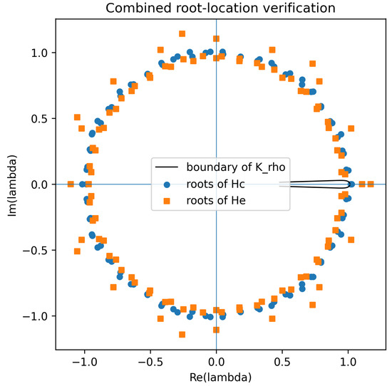
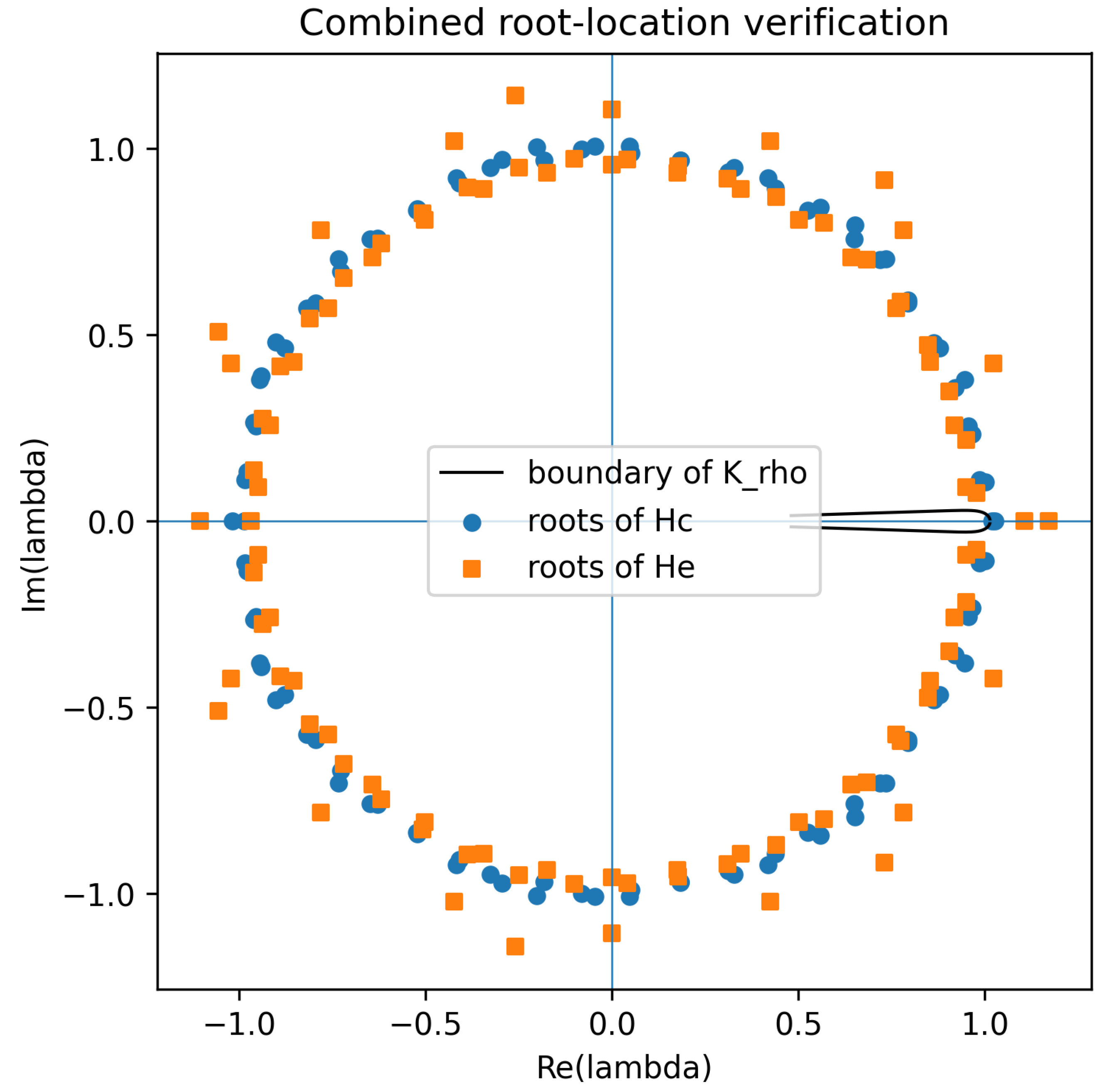
The computed characteristic roots of both $H_e$ and $H_c$ are shown in Figure 1. For the observer model, all 100 roots lie outside $K_{\rho }$, with minimum and maximum moduli approximately $0.9514$ and $1.1717$, respectively. For the full-state closed-loop model, all 100 roots also lie outside $K_{\rho }$, with minimum and maximum moduli approximately $0.9857$ and $1.0277$, respectively. Thus, the numerical root-location test confirms the hypotheses of Proposition 2 and Proposition 3.

Figure 1. Characteristic-root verification for the linearized observer and full-state closed-loop models. The roots associated with $H_e$ and $H_c$ lie outside the forbidden region $K_{\rho }$, which confirms the local linearized incommensurate stability conditions used in the gain design. The black curve denotes the boundary of $K_{\rho }$, while the blue and orange markers denote the full-state and observer-error roots, respectively.

4.2. Uncontrolled Benchmark Dynamics

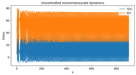
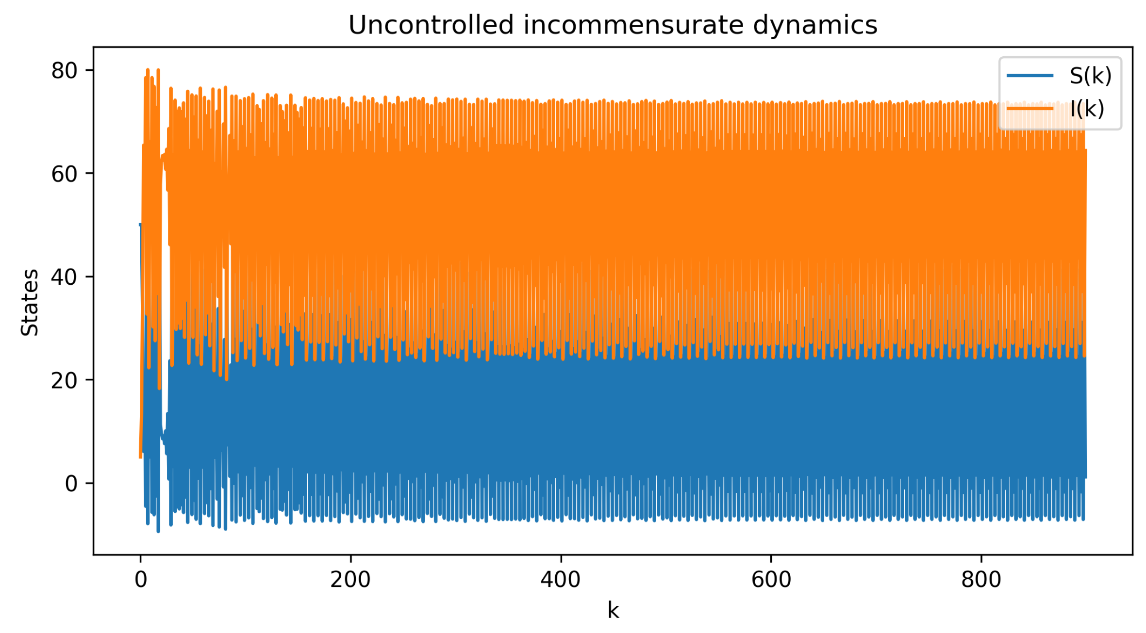
The uncontrolled incommensurate fractional-order SI benchmark is simulated first. Figure 2 shows that the infected compartment is not suppressed in the absence of mitigation. Instead, the trajectory exhibits large-amplitude oscillatory behavior. At the final simulation index, the uncontrolled trajectory satisfies

$$S\left(N\right)\approx 1.1466,I\left(N\right)\approx 64.3742,$$

(102)

with peak infected level

$$\underset{0\le k\le N}{max}I\left(k\right)\approx 80.0258.$$

(103)

The tail mean of $\left|I\right(k\left)\right|$ is approximately $51.2726$, which confirms that the infection persists over the simulated horizon. This uncontrolled behavior motivates the use of feedback control.

Figure 2. Uncontrolled dynamics of the incommensurate fractional-order SI benchmark model. The infected state remains large and oscillatory, showing that the virus-free equilibrium is not reached without mitigation.

4.3. Fractional-Order Selection Experiment

To address the reproducibility of the fractional-order choice, we next perform a loss-based order-selection experiment. Because the present manuscript treats the model as a normalized benchmark and no external cyber-epidemic telemetry is used in this numerical section, a synthetic infected-state telemetry signal is generated from the benchmark model and then used only to demonstrate the identification procedure. Thus, this experiment should not be interpreted as real malware-outbreak validation. Its purpose is to show how the fractional orders can be selected systematically rather than assigned arbitrarily.

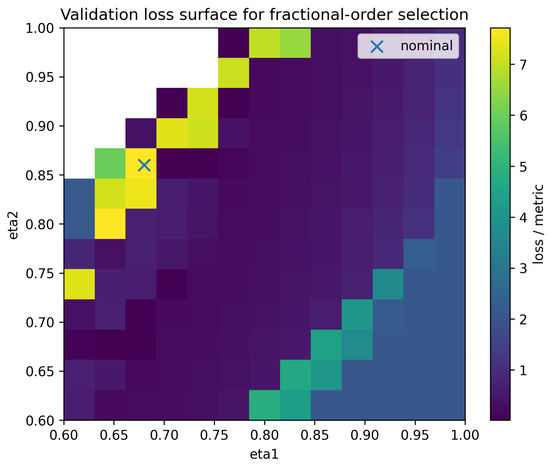
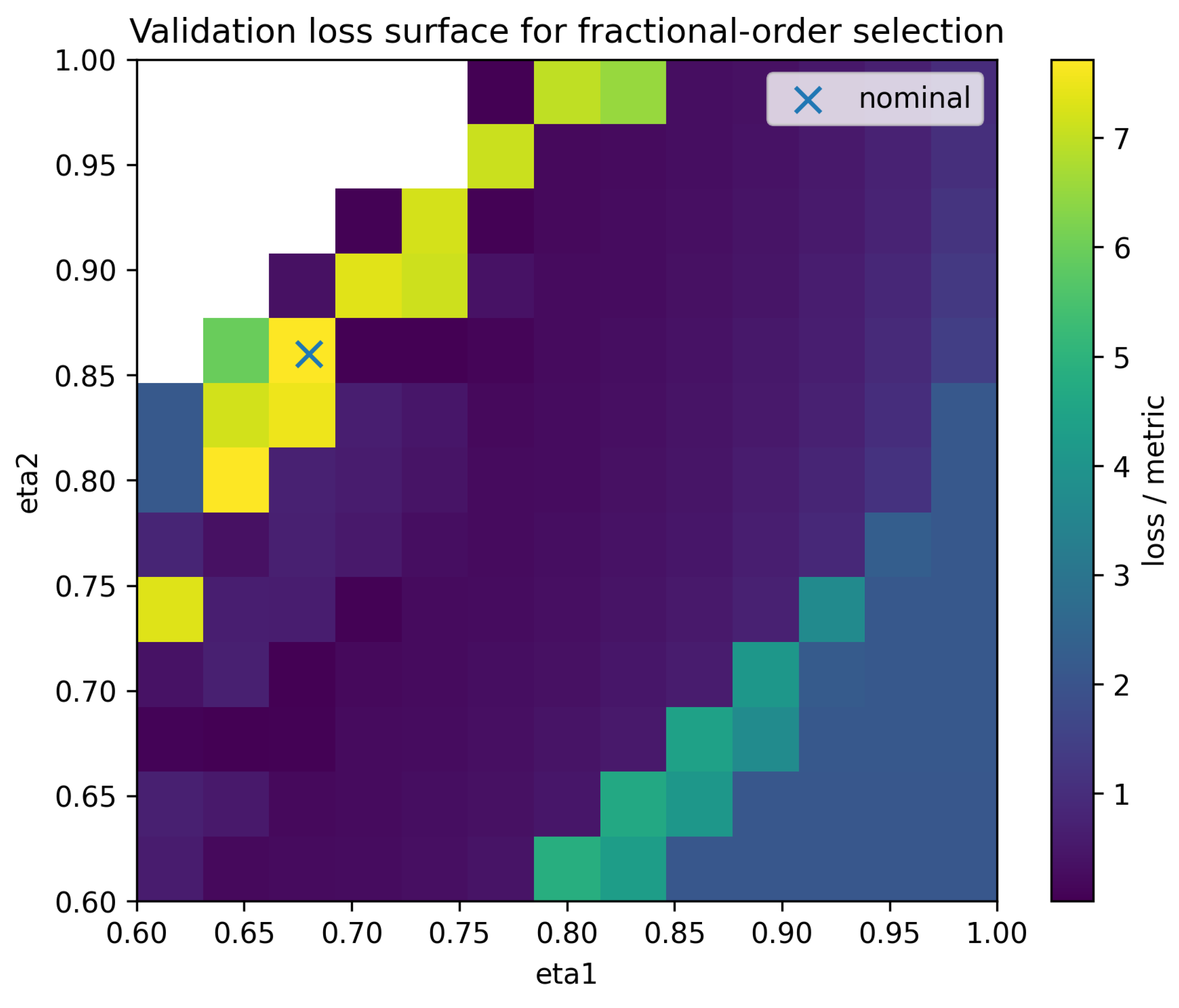
For each candidate pair $({\eta }_1,{\eta }_2)$ on a grid in $[0.6,1]\times [0.6,1]$, the model is simulated and the discrepancy between the simulated infected signal and the reference telemetry is measured. The loss is computed separately over a training segment and a validation segment. The validation-loss surface is shown in Figure 3. The minimum validation loss is obtained at

$$({\eta }_1,{\eta }_2)=(0.70,0.8667),$$

(104)

with training loss $0.2091$ and validation loss $0.01439$. This selected pair is close to the nominal values $(0.68,0.86)$ used in the remaining simulations. The result, therefore, supports the interpretation that the selected incommensurate orders are reproducible model parameters within the proposed loss-based identification framework.

Figure 3. Validation-loss surface for the fractional-order selection experiment. The loss-based procedure selects $({\eta }_1,{\eta }_2)=(0.70,0.8667)$, which is close to the nominal incommensurate orders $(0.68,0.86)$. The experiment illustrates a systematic order-selection procedure; it is not claimed as real malware-data validation.

4.4. Closed-Loop Comparison

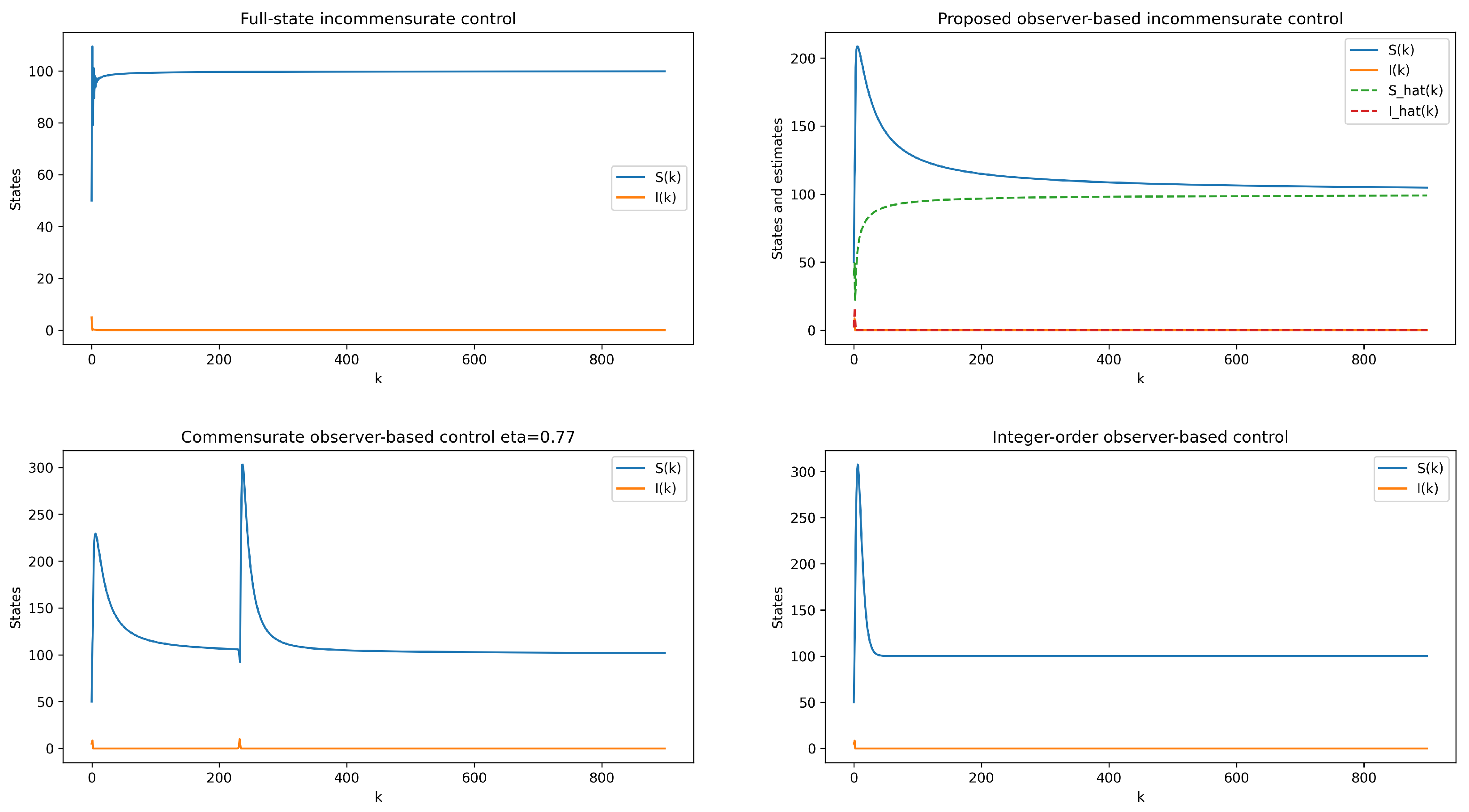
We now compare the uncontrolled benchmark, the full-state incommensurate controller, the proposed observer-based incommensurate controller, and two fractional-order baselines. The first baseline is a commensurate fractional observer-based controller with ${\eta }_1={\eta }_2=0.77$. The second is an integer-order observer-based implementation with ${\eta }_1={\eta }_2=1$. The purpose of these comparisons is not to claim universal superiority, but to assess the effect of the incommensurate memory structure and the observer-based implementation under the same benchmark setting. This additional set of contrast examples was included to make the numerical evidence more persuasive, as it compares the proposed incommensurate observer-based controller with both commensurate fractional and integer-order alternatives.

The quantitative comparison is reported in Table 1. The uncontrolled system has a large final infected level and a large tail mean infection. The full-state controller strongly reduces the infected level, with $I\left(N\right)\approx 1.95\times {10}^{-3}$ over the present finite horizon. The proposed observer-based controller drives $I\left(N\right)$ to zero and reaches $S\left(N\right)\approx 104.70$, which is within the prescribed neighborhood of the target $S^{★}=100$. The commensurate and integer-order observer-based baselines also suppress the infected state, but they display different transient behavior and different control-energy requirements. In particular, the commensurate case requires a larger control energy in this experiment, while the integer-order case produces a sharper transient in the susceptible channel.

Table 1. Baseline comparison over the reported simulation horizon. The success criterion requires suppression of the infected compartment and convergence of the susceptible state to a prescribed neighborhood of $S^{★}$. Control energy is computed as ${\sum }_k(G_1{\left(k\right)}^2+G_2{\left(k\right)}^2)$.

Case	S(N)	I(N)	max I(k)	Tail Mean |I|	Control Energy
Uncontrolled incommensurate	1.1466	64.3742	80.0258	51.2726	0
Full-state incommensurate	99.8519	$1.9466\times {10}^{-3}$	5.0000	$2.1379\times {10}^{-3}$	$4.7895\times {10}^3$
Proposed observer-based incommensurate	104.6972	0	8.5900	0	$5.2159\times {10}^4$
Observer-based commensurate	101.8750	0	10.2489	0	$1.2378\times {10}^5$
Observer-based integer-order	100.0000	0	8.5900	0	$3.5762\times {10}^4$

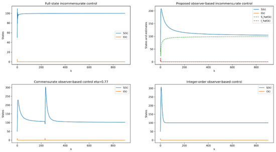
Figure 4 confirms the quantitative results in Table 1. In the proposed observer-based case, the infected state is rapidly suppressed using only the infected-state measurement. The susceptible state exhibits a larger transient than in the full-state case because the controller acts through the estimated state and the susceptible compartment is not directly measured. The apparently very fast settling of the infected component should be interpreted carefully. It is caused by the combined effect of the direct infected-state measurement, the relatively large correction gain ${\mathcal{\ell }}_2=4.0$, the cancellation terms in the feedback law, and the initial saturated mitigation action. It does not mean that the nonlinear fractional closed loop has finite-time stability or global convergence; it only shows rapid finite-horizon suppression for the selected benchmark parameters and initial conditions.

Figure 4. Closed-loop comparison. (Top left): full-state incommensurate feedback. (Top right): proposed observer-based incommensurate feedback. (Bottom left): commensurate fractional observer-based baseline. (Bottom right): integer-order observer-based baseline. All controlled cases suppress the infected state, but the transient behavior and control effort differ significantly. The horizontal axis is the update index k, and the vertical axis gives the corresponding state or estimate level.

4.5. Observer Performance and Control Effort

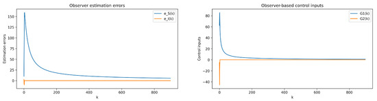
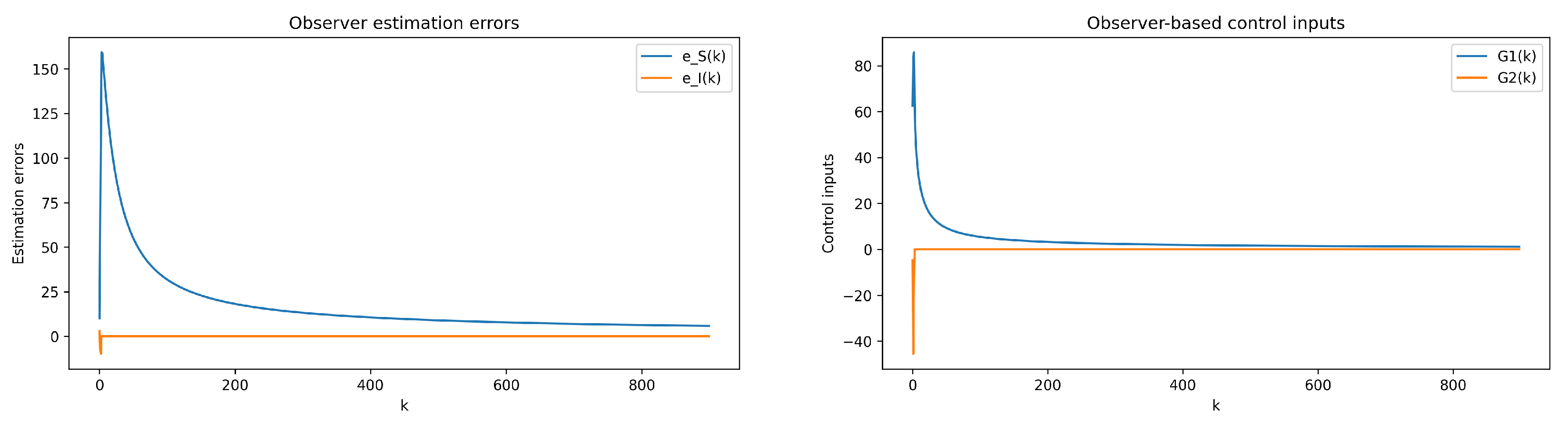
The estimation errors and control signals of the proposed observer-based incommensurate controller are shown in Figure 5. The infected-state estimation error converges to a negligible level, whereas the susceptible-state estimation error exhibits a larger transient and a slower decay. This behavior is consistent with the infected-only measurement structure: the measured channel directly corrects $\widehat{I}\left(k\right)$, while $\widehat{S}\left(k\right)$ is reconstructed only indirectly through the nonlinear coupling and the observer innovation.

Figure 5. Observer-based incommensurate closed-loop performance. (Left): estimation errors $e_S\left(k\right)=S\left(k\right)-\widehat{S}\left(k\right)$ and $e_I\left(k\right)=I\left(k\right)-\widehat{I}\left(k\right)$. (Right): saturated control inputs $G_1\left(k\right)$ and $G_2\left(k\right)$. The infected error becomes negligible, while the susceptible error displays a larger transient due to infected-only measurements. The notation in the legend is chosen to match the variables used in the theoretical development.

This result is important for interpreting the practical value and limitations of the observer. The proposed observer is effective for reconstructing the measured infected channel and for enabling infection suppression. However, because the susceptible compartment is not directly measured, the susceptible estimate should not be interpreted as having uniformly fast transient accuracy over all initial conditions. This observation is consistent with the local and benchmark-oriented scope of the theoretical results. Thus, the rapid decay of $I\left(k\right)$ and $\widehat{I}\left(k\right)$ in the plotted trajectories is a controlled transient phenomenon rather than an additional theoretical stability claim.

4.6. Robustness to Measurement Noise, Missing Data, and Process Disturbances

To examine robustness, the measurement equation is perturbed as

$$y\left(k\right)=I\left(k\right)+\nu \left(k\right),$$

(105)

where $\nu \left(k\right)$ is a zero-mean measurement noise sequence. Missing measurements are also considered by randomly removing a prescribed fraction of infected-state samples and using a zero-order-hold reconstruction of the last available measurement. Finally, bounded process disturbances are added to the plant update terms. Each robustness configuration is repeated three times with different random seeds.

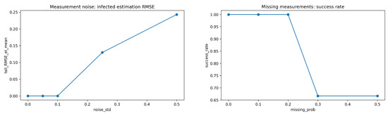
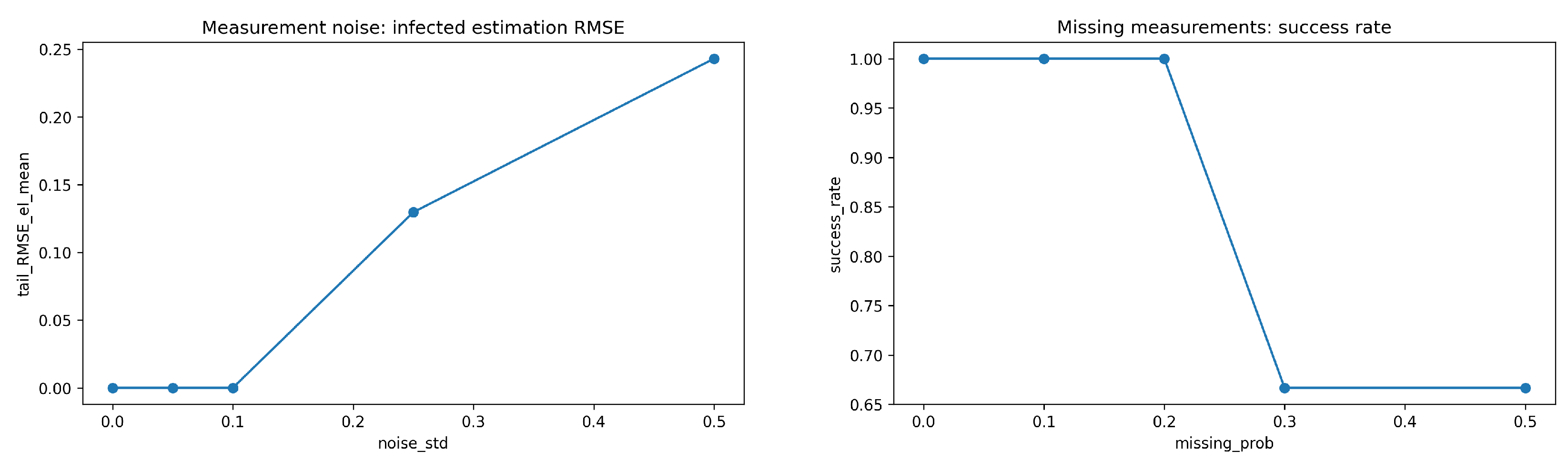
The robustness results are summarized in Table 2. For measurement noise, the closed loop maintains a $100\%$ success rate for all tested standard deviations up to $\sigma =0.5$. The final infected level remains zero in all reported averages, although the infected-state estimation RMSE increases for larger noise. For missing measurements, the method remains successful for moderate missingness up to $20\%$, but the success rate decreases to $66.7\%$ when the missing probability is $30\%$ or $50\%$. This indicates that the observer-based controller tolerates moderate data loss but is not insensitive to severe measurement unavailability. For process disturbances up to a standard deviation of $0.1$, the final infected level remains zero and the success rate remains $100\%$.

Table 2. Robustness summary. Success rate is computed over three random seeds. The reported RMSE values are tail RMSEs over the last part of the simulation horizon.

Test	Level	Success Rate	Final I Mean	Peak I Mean	Tail RMSE ${\mathit{e}}_{\mathit{I}}$
Measurement noise $\sigma =0$	0	1.000	0	8.5900	${10}^{-9}$
Measurement noise $\sigma =0.10$	0.10	1.000	0	8.5900	${10}^{-9}$
Measurement noise $\sigma =0.25$	0.25	1.000	0	8.5900	0.1297
Measurement noise $\sigma =0.50$	0.50	1.000	0	8.5900	0.2430
Missing measurements $p=0.10$	0.10	1.000	0	53.3178	${10}^{-9}$
Missing measurements $p=0.20$	0.20	1.000	0	116.3283	${10}^{-9}$
Missing measurements $p=0.30$	0.30	0.667	0	107.8400	${10}^{-9}$
Missing measurements $p=0.50$	0.50	0.667	0	107.8400	${10}^{-9}$
Process disturbance ${\sigma }_w=0.10$	0.10	1.000	0	8.5928	${10}^{-9}$

In Figure 6, the method is robust to measurement noise and moderate missingness, but performance degrades when a large fraction of infected-state measurements is unavailable.

Figure 6. Robustness of the proposed observer-based controller. (Left): tail RMSE of the infected-state estimation error under increasing measurement noise. (Right): success rate under increasing missing-measurement probability.

4.7. Parameter and Fractional-Order Sensitivity

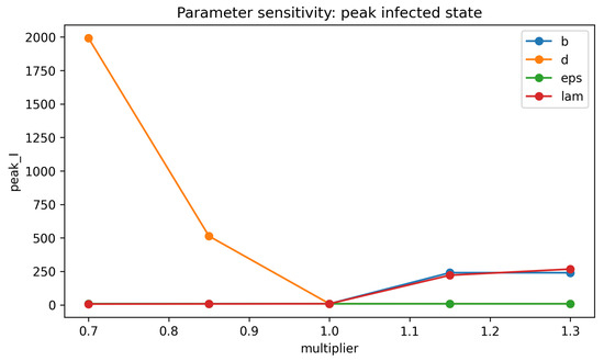
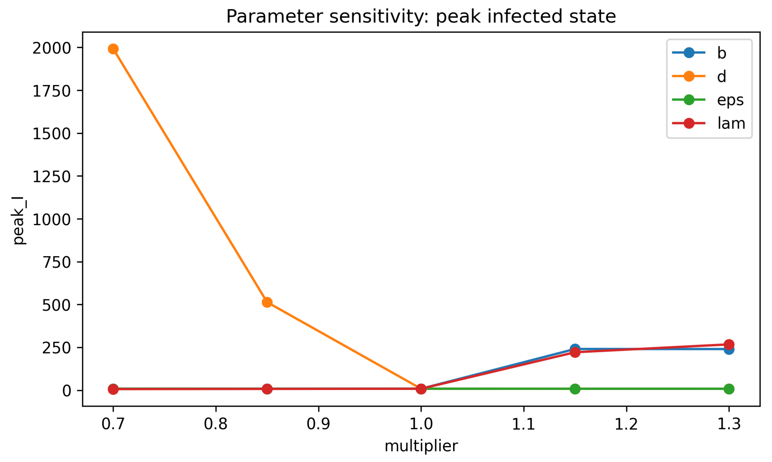
The next experiment examines the sensitivity of the nonlinear closed loop to parameter and fractional-order variations. Each parameter $b,\lambda ,d,ϵ$ is varied multiplicatively while the controller and observer gains are kept fixed. When b or d is varied, the virus-free target $S^{★}=b/d$ also changes; therefore, the following discussion focuses on the infected-state response and the peak transient rather than on a fixed nominal susceptible target.

Figure 7 shows that the peak infected transient is most sensitive to the recruitment parameter b, the infection coefficient $\lambda$, and the removal/disconnection coefficient d. In particular, reducing d produces the most severe transient amplification in the tested range. By contrast, variations of $ϵ$ have a milder effect on the peak infected response. These results indicate that the proposed gains are effective near the nominal benchmark point but should be retuned if the removal/disconnection rate or the infection coefficient changes substantially.

Figure 7. Parameter sensitivity of the proposed observer-based closed loop. The peak infected level is especially sensitive to variations of b, $\lambda$, and d, whereas the tested variations of $ϵ$ produce a smaller effect.

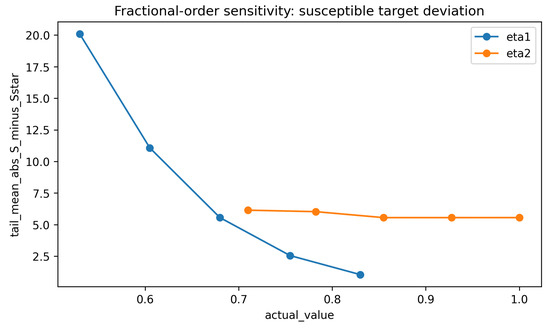
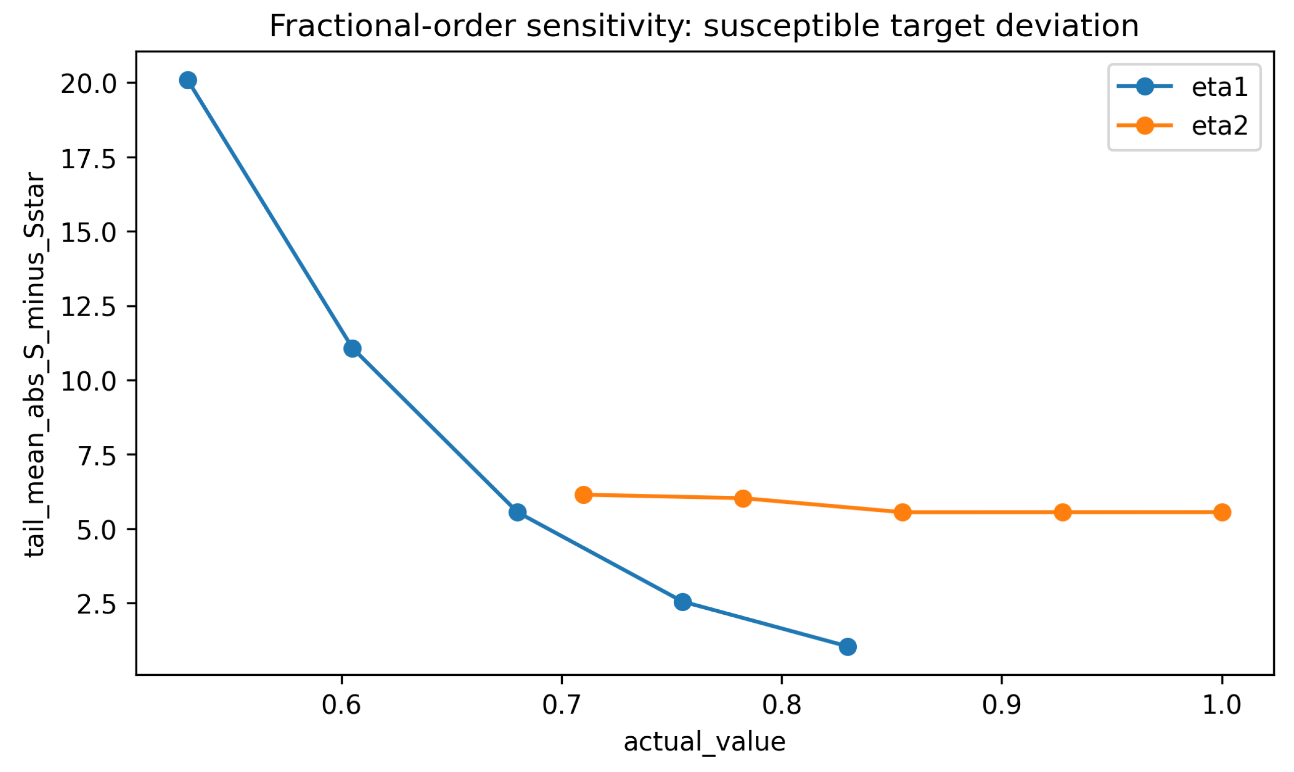
The influence of the fractional orders is summarized in Figure 8. Across the tested order variations, the infected state is generally suppressed, but the deviation of the susceptible state from its target is affected by the memory orders. This observation supports the importance of treating ${\eta }_1$ and ${\eta }_2$ as meaningful design and identification parameters rather than arbitrary numerical constants.

Figure 8. Fractional-order sensitivity of the observer-based closed loop. Although the infected state is suppressed in the tested order range, the final susceptible target deviation depends on the memory orders. This reinforces the need for a systematic order-selection procedure.

4.8. Numerical Attraction-Region Study

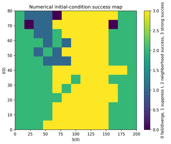
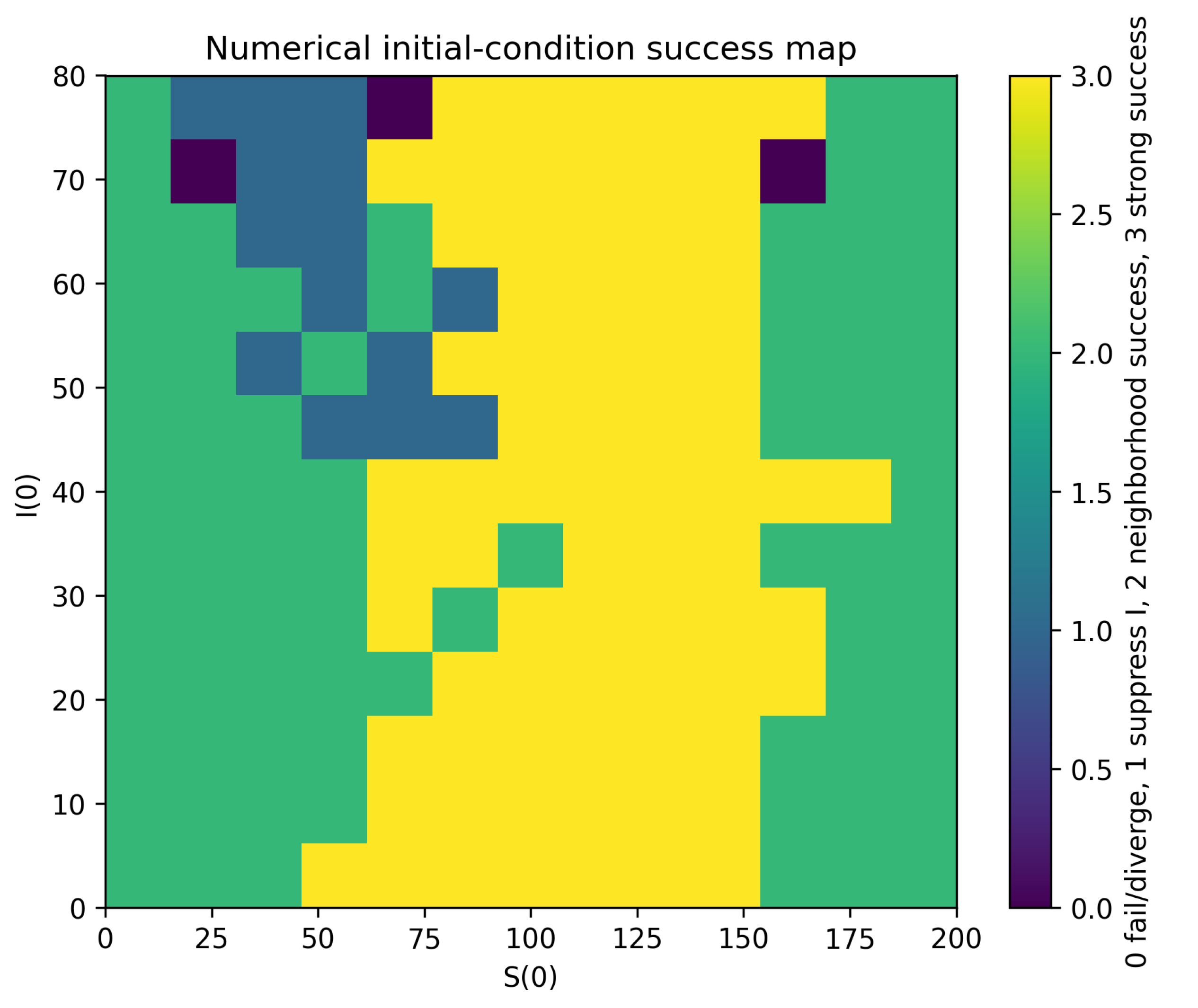
Finally, we perform a numerical initial-condition sweep to assess the nonlinear validity domain of the local linearized design. The initial susceptible and infected levels are varied over a two-dimensional grid, and the observer-based closed loop is simulated for each grid point. This experiment is not a formal analytical proof of a region of attraction. Instead, it provides a numerical map of the initial conditions for which the proposed controller suppresses the infected state and brings the susceptible state close to the virus-free target.

Each grid point is classified into one of four categories:

• status 0: failure or divergence;
• status 1: infected state suppressed but susceptible target neighborhood not reached;
• status 2: neighborhood success;
• status 3: strong success.

The resulting map is shown in Figure 9. Out of 169 tested initial conditions, 3 points are classified as failure or divergence, 14 points as infection suppression without susceptible-neighborhood success, 78 points as neighborhood success, and 74 points as strong success. Thus, $152/169$, approximately $89.9\%$, of the tested grid points satisfy the two stronger success categories, while $166/169$, approximately $98.2\%$, achieve at least infection suppression in the adopted classification. These results support the practical relevance of the local linearized design over a broad numerical set of initial conditions, while also confirming that the method should not be interpreted as globally stabilizing. In fact, Table 3 presents the Summary of the numerical initial-condition sweep.

Figure 9. Numerical initial-condition success map for the proposed observer-based incommensurate controller. The map gives a numerical estimate of the effective attraction region of the local design. Most tested initial conditions achieve neighborhood or strong success, while a small subset fails or does not reach the susceptible target neighborhood within the finite horizon.

Table 3. Summary of the numerical initial-condition sweep.

Status	Count	Fraction
0: failure/divergence	3	0.0178
1: infection suppressed only	14	0.0828
2: neighborhood success	78	0.4615
3: strong success	74	0.4379

4.9. Discussion of Numerical Findings

The expanded numerical study leads to the following conclusions. First, the characteristic-root computations confirm the local linearized design conditions for both the observer and full-state feedback matrices. Second, the uncontrolled incommensurate fractional-order benchmark exhibits persistent infected-state oscillations, whereas the controlled configurations suppress the infection. Third, the loss-based order-selection experiment provides a reproducible procedure for selecting $({\eta }_1,{\eta }_2)$, with the selected pair close to the nominal orders used in the benchmark simulations. Fourth, the observer-based controller remains effective under measurement noise, process disturbances, and moderate missing-data levels, although high missingness degrades the success rate. Fifth, the initial-condition sweep provides a numerical attraction-region assessment and confirms that the proposed method has a broad but not global nonlinear validity domain.

These findings directly support the theoretical positioning of the paper. The root-location plots validate the linearized incommensurate stability conditions, whereas the nonlinear simulations examine the behavior that is not covered by the local characteristic-root analysis. Therefore, the numerical evidence should be interpreted as a robustness and nonlinear-performance assessment of a local linearized observer-based design, not as a proof of global stabilization. The results also clarify the practical limitations of the approach: the susceptible state can display larger observer transients because only infected-state measurements are used, and the gains may require retuning under large changes of the infection or removal parameters.

5. Conclusions

This paper has presented an observer-based output-feedback stabilization framework for a normalized incommensurate fractional-order discrete-time SI benchmark model of computer-virus propagation. The model is treated as a dimensionless benchmark rather than as a predictive malware-forecasting tool. To improve practical interpretability, the revised formulation includes a parameter- and fractional-order identification pathway based on normalized infection telemetry, loss minimization, and model comparison.

The theoretical results are deliberately local. The observer, full-state feedback law, and observer-based controller are designed through characteristic-root conditions for the corresponding linearized incommensurate Caputo-like fractional difference systems. The infected-only measurement assumption is interpreted as a detectability-based cyber-monitoring configuration, and the nonlinear residuals, measurement-noise channel, missing-data formulation, and saturation caveat are made explicit. Thus, the paper does not claim global nonlinear stabilization or a global separation principle.

The numerical section supports these claims by verifying the root-location conditions, comparing the proposed design with full-state, commensurate fractional, and integer-order baselines, and testing robustness to measurement noise, missing data, process disturbances, parameter variations, and fractional-order changes. The initial-condition sweep provides a numerical estimate of the effective attraction region and confirms that the method has a broad finite-horizon validity for the benchmark setting, while also revealing limitations under severe missing data and large parameter deviations. Future work will focus on applying the calibration procedure for real-time-resolved malware telemetry and on developing stronger nonlinear robustness tools for incommensurate fractional-difference observer-based systems.

References

- Szor, P. The Art of Computer Virus Research and Defense; Addison-Wesley: Boston, MA, USA, 2005. [Google Scholar]
- Cohen, F. Computer viruses: Theory and experiments. Comput. Secur. 1987, 6, 22–35. [Google Scholar] [CrossRef] [Scilit]
- Kephart, J.O.; White, S.R. Directed-graph epidemiological models of computer viruses. In Proceedings of the 1991 IEEE Symposium on Security and Privacy, Oakland, CA, USA, 20–22 May 1991; pp. 343–359. [Google Scholar]
- Mishra, B.K.; Jha, N. Seiqrs model for the transmission of malicious objects in computer network. Appl. Math. Model. 2010, 34, 710–715. [Google Scholar] [CrossRef] [Scilit]
- Gan, C.; Yang, X.; Liu, W.; Zhu, Q. A propagation model of computer virus with nonlinear vaccination probability. Commun. Nonlinear Sci. Numer. Simul. 2014, 19, 92–100. [Google Scholar] [CrossRef] [Scilit]
- Yang, L.X.; Yang, X. The spread of computer viruses under the influence of removable storage devices. Appl. Math. Comput. 2012, 219, 3914–3922. [Google Scholar] [CrossRef] [Scilit]
- Ren, J.; Yang, X.; Zhu, Q.; Yang, L.-X.; Zhang, C. A novel computer virus model and its dynamics. Nonlinear Anal. Real. World Appl. 2012, 13, 376–384. [Google Scholar] [CrossRef] [Scilit]
- Dordević, M.; Dordević, J. Sirs model for computer viruses propagation with time-dependent delay and jumps. Filomat 2025, 39, 2525–2556. [Google Scholar] [CrossRef] [Scilit]
- Almatroud, O.A.; Hammad, M.A.; Dababneh, A.; Diabi, L.; Ouannas, A.; Khennaoui, A.A.; Alshammari, S. Multistability, chaos, and synchronization in novel symmetric difference equation. Symmetry 2024, 16, 1093. [Google Scholar] [CrossRef] [Scilit]
- Li, C.; Chen, Y.; Kurths, J. Fractional calculus and its applications. Philos. Trans. R. Soc. A Math. Phys. Eng. Sci. 2013, 371, 20130037. [Google Scholar] [CrossRef] [Scilit]
- Podlubny, I. Fractional Differential Equations; Academic Press: Boca Raton, FL, USA, 1998. [Google Scholar]
- Diethelm, K. The Analysis of Fractional Differential Equations; Springer: Berlin/Heidelberg, Germany, 2010. [Google Scholar]
- Abdeljawad, T. On riemann and caputo fractional differences. Comput. Math. Appl. 2011, 62, 1602–1611. [Google Scholar] [CrossRef] [Scilit]
- Atici, F.M.; Eloe, P. Discrete fractional calculus with the nabla operator. Electron. J. Qual. Theory Differ. Equ. 2009, 62, 3. [Google Scholar] [CrossRef] [Scilit]
- Anastassiou, G.A. Principles of delta fractional calculus on time scales and inequalities. Math. Comput. Model. 2010, 52, 556–566. [Google Scholar] [CrossRef] [Scilit]
- Čermák, J.; Gyori, I.; Nechvátal, L. On explicit stability conditions for a linear fractional difference system. Fract. Calc. Appl. Anal. 2015, 18, 651–672. [Google Scholar] [CrossRef] [Scilit]
- Baleanu, D.; Wu, G.; Bai, Y.; Chen, F. Stability analysis of caputo-like discrete fractional systems. Commun. Nonlinear Sci. Numer. Simul. 2017, 48, 520–530. [Google Scholar] [CrossRef] [Scilit]
- Shatnawi, M.T.; Djenina, N.; Ouannas, A.; Batiha, I.M.; Grassi, G. Novel convenient conditions for the stability of nonlinear incommensurate fractional-order difference systems. Alex. Eng. J. 2022, 61, 1655–1663. [Google Scholar] [CrossRef] [Scilit]
- Djenina, N.; Ouannas, A.; Batiha, I.M.; Grassi, G.; Pham, V.T. On the stability of linear incommensurate fractional-order difference systems. Mathematics 2020, 8, 1754. [Google Scholar] [CrossRef] [Scilit]
- Djenina, N.; Ouannas, A. Stability and stabilisation of nonlinear incommensurate fractional order difference systems. In State Estimation and Stabilization of Nonlinear Systems: Theories and Applications; Springer International Publishing: Cham, Switzerland, 2023; pp. 147–168. [Google Scholar]
- Batiha, I.M.; Ogilat, O.; Bendib, I.; Ouannas, A.; Jebril, I.H.; Anakira, N. Finite-time dynamics of the fractional-order epidemic model: Stability, synchronization, and simulations. Chaos Solitons Fractals X 2024, 13, 100118. [Google Scholar] [CrossRef] [Scilit]
- Batiha, I.M.; Hijazi, M.S.; Hioual, A.; Ouannas, A.; Odeh, M.; Momani, S. Stability analysis and numerical simulations of a discrete-time epidemic model. Partial Differ. Equ. Appl. Math. 2025, 13, 101118. [Google Scholar] [CrossRef] [Scilit]
- Almatroud, A.O.; Djenina, N.; Ouannas, A.; Grassi, G. The seir covid-19 model described by fractional-order difference equations: Analysis and application with real data in brazil. J. Differ. Equ. Appl. 2023, 29, 1467–1479. [Google Scholar] [CrossRef] [Scilit]
- Dababneh, A.; Djenina, N.; Ouannas, A.; Grassi, G.; Batiha, I.M.; Jebril, I.H. A new incommensurate fractional-order discrete COVID-19 model with vaccinated individuals compartment. Fractal Fract. 2022, 6, 456. [Google Scholar] [CrossRef] [Scilit]
- Ouannas, A.; Mesdoui, F.; Momani, S.; Batiha, I.; Grassi, G. Synchronization of fitzhugh–nagumo reaction–diffusion systems via one-dimensional linear control law. Arch. Control Sci. 2021, 31, 189–202. [Google Scholar] [CrossRef] [Scilit]
- Mesdoui, F.; Shawagfeh, N.; Ouannas, A. Global synchronization of fractional-order and integer-order n component reaction diffusion systems: Application to biochemical models. Math. Methods Appl. Sci. 2021, 44, 1003–1012. [Google Scholar] [CrossRef] [Scilit]
- Bendib, I.; Ouannas, A.; Dalah, M. Mittag-leffler synchronization of fractional-order reaction-diffusion systems. Asian J. Control 2025, 28, 279–293. [Google Scholar] [CrossRef] [Scilit]
- Ouannas, A.; Batiha, I.M.; Pham, V.T. Fractional Discrete Chaos: Theories, Methods and Applications; World Scientific: Singapore, 2023. [Google Scholar] [CrossRef] [Scilit]
- Talbi, I.; Ouannas, A.; Khennaoui, A.A.; Berkane, A.; Batiha, I.M.; Grassi, G.; Pham, V.T. Different dimensional fractional-order discrete chaotic systems based on the caputo h-difference discrete operator: Dynamics, control, and synchronization. Adv. Differ. Equ. 2020, 2020, 556. [Google Scholar] [CrossRef] [Scilit]
- Khennaoui, A.A.; Ouannas, A.; Boulaaras, S.; Pham, V.T.; Azar, A.T. A fractional map with hidden attractors: Chaos and control. Eur. Phys. J. Spec. Top. 2020, 229, 1083–1093. [Google Scholar] [CrossRef] [Scilit]
- Al-Taani, H.; Hammad, M.A.; Abudayah, M.; Diabi, L.; Ouannas, A. On fractional discrete memristive model with incommensurate orders: Symmetry, asymmetry, hidden chaos and control approaches. Symmetry 2025, 17, 143. [Google Scholar] [CrossRef] [Scilit]
- Ouannas, A.; Ahmed, S.B.; Grassi, G.; Horani, M.A.; Khennaoui, A.A.; Hioual, A. The fractional variable-order grassi–miller map: Chaos, complexity, and control. Comput. Math. Methods 2025, 2025, 6674521. [Google Scholar] [CrossRef] [Scilit]
- Ouannas, A.; Khennaoui, A.A.; Batiha, I.M.; Pham, V.T. Stabilization of different dimensional fractional chaotic maps. In Fractional-Order Design; Academic Press: Cambridge, MA, USA, 2022; pp. 123–155. [Google Scholar]
- Almatroud, A.O.; Ouannas, A.; Grassi, G.; Batiha, I.M.; Gasri, A.; Al-Sawalha, M.M. Different linear control laws for fractional chaotic maps using lyapunov functional. Arch. Control Sci. 2021, 31, 765–780. [Google Scholar] [CrossRef] [Scilit]
- Zarour, A.; Ouannas, A.; Latrous, C.; Berkane, A. Linear chaos control of fractional generalized hénon map. Nonlinear Dyn. Syst. Theory 2021, 21, 216–224. [Google Scholar]
- Khennaoui, A.A.; Ouannas, A.; Bendoukha, S.; Grassi, G.; Wang, X.; Pham, V.-T.; Alsaadi, F.E. Chaos, control, and synchronization in some fractional-order difference equations. Adv. Differ. Equ. 2019, 2019, 412. [Google Scholar] [CrossRef] [Scilit]
- Khennaoui, A.A.; Ouannas, A.; Bendoukha, S.; Grassi, G.; Lozi, R.P.; Pham, V.T. On fractional-order discrete-time systems: Chaos, stabilization and synchronization. Chaos Solitons Fractals 2019, 119, 150–162. [Google Scholar] [CrossRef] [Scilit]
- Azar, A.T.; Vaidyanathan, S.; Ouannas, A. (Eds.) Fractional Order Control and Synchronization of Chaotic Systems; Springer: Berlin/Heidelberg, Germany, 2017; Volume 688. [Google Scholar]
- Zouak, I.; Ouannas, A.; Khennaoui, A.A. A new fractional discrete memristive map with incommensurate order and hidden dynamics. In Fractional Calculus and Applications; Springer: Berlin/Heidelberg, Germany, 2025. [Google Scholar]
- Abu Hammad, M.; Zouak, I.; Ouannas, A.; Grassi, G. Fractional discrete computer virus system: Chaos and complexity algorithms. Algorithms 2025, 18, 444. [Google Scholar] [CrossRef] [Scilit]
- Zouak, I.; Alshanty, A.; Ouannas, A.; Mongelli, A.; Ciccarese, G.; Grassi, G. From continuous integer-order to fractional discrete-time: A new computer virus model with chaotic dynamics. Technologies 2025, 13, 471. [Google Scholar] [CrossRef] [Scilit]
- Kahouli, O.; Zouak, I.; Abu Hammad, M.; Ouannas, A.; Ayari, M. On an incommensurate chaotic fractional discrete model of a computer virus: Stabilization and synchronization. AIMS Math. 2025, 10, 19940–19957. [Google Scholar] [CrossRef] [Scilit]
- Kahouli, O.; Zouak, I.; Ouannas, A.; El Amraoui, L.; Ayari, M. On fractional discrete-time computer virus model: Stability, bifurcation, chaos and complexity analysis. Mathematics 2025, 13, 3272. [Google Scholar] [CrossRef] [Scilit]
- Aloui, A.; Zouak, I.; Kahouli, O.; Ouannas, A.; El Amraoui, L.; Ayari, M. Nonlinear dynamics of a discrete-time model for computer virus propagation: Chaos, complexity, stabilization, and synchronization. Mathematics 2025, 13, 3681. [Google Scholar] [CrossRef] [Scilit]
- Jebril, I.H.; Dibi, K.; Zouak, I.; Ouannas, A.; Khennaoui, A.-A.; Batiha, I.M. Incommensurate fractional computer virus system: Control and simulation. In Proceeding-12th International Conference on Information Technology; Institute of Electrical and Electronics Engineers Inc.: New York City, NJ, USA, 2025; pp. 109–113. [Google Scholar]
- Momani, S.; Zouak, I.; Batiha, I.; Ouannas, A.; Khennaoui, A.-A.; Momani, Z. Chaos synchronization in a fractional-order computer virus system with incommensurate dynamics. Adv. Math. Model. Appl. 2025, 10, 488–498. [Google Scholar]
- Oudetallah, J.; Zouak, I.; Audeh, W.; Ouannas, A.; Khennaoui, A.-A.; Batiha, I.M.; Momani, S. Synchronization of computer virus system using fractional calculus. In Proceedings of the 2025 1st International Conference on Computational Intelligence Approaches and Applications (ICCIAA), Amman, Jordan, 28–30 April 2025; pp. 1–6. [Google Scholar] [CrossRef] [Scilit]
- Oudetallah, J.; Zouak, I.; Audeh, W.; Ouannas, A.; Khennaoui, A.-A.; Batiha, I.M.; Momani, S. Control of chaos in fractional computer virus model. In Proceedings of the 2025 1st International Conference on Computational Intelligence Approaches and Applications (ICCIAA), Amman, Jordan, 28–30 April 2025; pp. 1–5. [Google Scholar]
- Kahouli, O.; Zouak, I.; Abu Hammad, M.; Ouannas, A. Chaos, control and synchronization in discrete time computer virus system with fractional orders. AIMS Math. 2025, 10, 13594–13621. [Google Scholar] [CrossRef] [Scilit]
- Kahouli, O.; Zouak, I.; Ouannas, A.; Abidi, I.; Bahou, Y.; Elgharbi, S.; Chaabane, M. Control and synchronization of chaos in some fractional computer virus models. Asian J. Control. 2026, 28, 240–248. [Google Scholar] [CrossRef] [Scilit]
- Naifar, O.; Boukettaya, G.; Ouali, A. Global stabilization of an adaptive observer-based controller design applied to induction machine. Int. J. Adv. Manuf. Technol. 2015, 81, 423–432. [Google Scholar] [CrossRef] [Scilit]
- Jmal, A.; Naifar, O.; Ben Makhlouf, A.; Derbel, N.; Hammami, M.A. Adaptive stabilization for a class of fractional-order systems with nonlinear uncertainty. Arab. J. Sci. Eng. 2020, 45, 2195–2203. [Google Scholar] [CrossRef] [Scilit]
- Zhou, C.; Zhu, B.; Song, X.; Liu, J.J.; Cui, Y.; Lam, J. Observer-based stabilization of positive linear system with disturbances. Int. J. Robust. Nonlinear Control 2026, 36, 732–746. [Google Scholar] [CrossRef] [Scilit]
- Cai, B.; Xu, K.; Ding, Y.; Zhang, L.; Wang, Y. Observer-based control for switched systems with limited statistical information. In IEEE Transactions on Systems, Man, and Cybernetics: Systems; IEEE: Piscataway, NJ, USA, 2026. [Google Scholar]
- Romano, C.; Borri, A.; Di Ferdinando, M.; Di Benedetto, M.D.; Pepe, P. Sampled-data observer-based exponential stabilization of nonlinear systems with an application to tumor control. Automatica 2026, 185, 112752. [Google Scholar] [CrossRef] [Scilit]
- Shen, G.; Wang, R.; Li, X.; Mao, J.; Xiang, Z. Observer-based predefined-time stabilizing control for nonlinear time-delay systems via dual-dynamic-gains method. Int. J. Robust. Nonlinear Control 2026, 36, 3708–3721. [Google Scholar] [CrossRef] [Scilit]
- Yang, X.; Zhou, B. Observer based memoryless output feedback stabilization for linear systems with both complex input and output time delays. J. Frankl. Inst. 2026, 363, 108481. [Google Scholar] [CrossRef] [Scilit]
- Debouza, M.; Errouissi, R.; Shareef, H. Disturbance observer-based voltage harmonic suppression in three-phase standalone inverters using -stability theory. Electr. Power Syst. Res. 2026, 254, 112564. [Google Scholar] [CrossRef] [Scilit]
- Fu, Y.; Ruan, J.; Fan, Y.; Fu, L. Observer-based optimal neuro-control for unknown nonlinear systems subject to input constraints via a dynamic event-triggered strategy. Int. J. Robust. Nonlinear Control 2026, 36, 2461–2473. [Google Scholar] [CrossRef] [Scilit]
- Sun, P.; Wang, C.; Lu, H.; Li, A.; Zabolotnov, Y. Disturbance observer-based fixed-time control for space tether system with prescribed performance after capturing debris. Astrodynamics 2026, 10, 123–137. [Google Scholar] [CrossRef] [Scilit]
- Yang, X.; Zhu, Q.; Wang, H. Observer-based event-triggered control for stochastic systems with sampled-data output. In IEEE Transactions on Systems, Man, and Cybernetics: Systems; IEEE: Piscataway, NJ, USA, 2026. [Google Scholar]
- Brandibur, O.; Kaslik, E.; Mozyrska, D.; Wyrwas, M. Stability results for two-dimensional systems of fractional-order difference equations. Mathematics 2020, 8, 1751. [Google Scholar] [CrossRef] [Scilit]
- Franco-Perez, L.; Fernandez-Anaya, G.; Quezada-Tellez, L.A. On stability of nonlinear nonautonomous discrete fractional caputo systems. J. Math. Anal. Appl. 2020, 487, 124021. [Google Scholar] [CrossRef] [Scilit]
- Batiha, I.M.; Bendib, I.; Ouannas, A.; Jebril, I.H.; Alkhazaleh, S.; Momani, S. On new results of stability and synchronization in finite-time for fitzhugh–nagumo model using gronwall inequality and lyapunov function. J. Robot Control 2024, 5, 1897–1909. [Google Scholar]
Disclaimer/Publisher’s Note: The statements, opinions and data contained in all publications are solely those of the individual author(s) and contributor(s) and not of MDPI and/or the editor(s). MDPI and/or the editor(s) disclaim responsibility for any injury to people or property resulting from any ideas, methods, instructions or products referred to in the content. |
© 2026 by the authors. Licensee MDPI, Basel, Switzerland. This article is an open access article distributed under the terms and conditions of the Creative Commons Attribution (CC BY) license.