Image-Based Visual Servoing of Quadrotor MAVs Using Model Predictive Control with Velocity Observation and State Update

Abstract

A model predictive control (MPC) strategy is proposed based on state observation and updating for image-based visual servoing (IBVS) tasks of micro aerial vehicles (MAVs). This control strategy enables precise pose adjustment of MAVs without relying on the global positioning system (GPS). Specifically, image features are first defined on a virtual image plane to decouple the translational motion of the MAV. Subsequently, a linear velocity observer is developed to provide high-quality real-time velocity information for the MAV during IBVS execution. Furthermore, the image dynamics on the virtual image plane are linearized using a first-order Taylor expansion, and a linear MPC controller is formulated to efficiently compute the optimal control inputs. Moreover, the state inputs to the MPC controller are updated at each control cycle to eliminate errors accumulated during the rolling optimization based on the linearized dynamics, thereby ensuring the precision of IBVS. Simulation and experimental results demonstrate the performance of the proposed observer and control strategy.

1. Introduction

Owing to their advantages such as compact structure and high maneuverability, quadrotor micro aerial vehicles (MAVs) have attracted extensive research attention for their excellent performance in executing tasks such as tracking, hovering, and landing in complex indoor and outdoor environments. The motion control of MAVs has also played a significant role in applications including exploration, rescue, and reconnaissance. Substantial results have been reported [1,2,3]. MAVs are typically equipped with a global positioning system (GPS) and an inertial measurement unit (IMU) as part of their sensor system. Although the GPS offers extensive coverage and high-precision positioning, its signal is often weak or unavailable in constrained environments such as indoors, tunnels, and valleys [4]. IMUs can provide reliable attitude and angular velocity information independently of external signals. However, they suffer from accumulated errors in acceleration and velocity measurements over time, which prevents them from delivering accurate position and linear velocity information [5]. In contrast, visual sensors are cost-effective and can provide rich environmental information.

Vision-based control techniques have provided novel solutions for autonomous flight of MAVs, playing a critical role in applications such as map reconstruction [6], state estimation [7], path planning [8], obstacle avoidance [9], autonomous landing [10], and visual servoing [11]. Image-based visual servoing (IBVS) is a motion control framework that relies on image information [12,13]. In IBVS, control inputs are derived from the feedback information of the target in the image, forming a closed-loop control system that exhibits robustness to camera models [14,15]. However, considering the inherent nonlinearity and underactuated physical characteristics of quadrotor MAVs, along with the strongly coupled geometric characteristics of the image dynamics, the application of IBVS to quadrotor MAVs remains significantly challenging [16].

To overcome the challenges associated with implementing IBVS schemes using quadrotor MAVs, various technical approaches have been developed. Among them, the spherical camera method [17] and the virtual camera method [18] represent two prevalent solutions. In the spherical camera method, spherical centroid data projected onto a spherical image space are utilized, and a cascaded nonlinear IBVS controller is designed by exploiting the passivity property of the feature error, thereby decoupling the position and orientation dynamics [19]. The virtual camera method typically employs image moment features [20] on a virtual image plane [21] to decouple image dynamics and eliminate the influence of roll and pitch motions. Compared with the spherical camera method, the virtual camera method demonstrates superior performance in addressing the strong coupling of image dynamics while further enhancing MAVs’ control performance along the vertical axis [22].

Building upon the virtual camera method, related research has achieved multifaceted progress in enhancing IBVS performance. In [23], a critical neural network structure was utilized to approximate errors, and an adaptive dynamic programming method for IBVS was developed. The work in [24] extended the IBVS scheme to the problem of tracking moving targets by designing a velocity observer to continuously estimate the unknown linear velocity of the target, thereby enabling robust target tracking under a motion control law. In [25], a state observer was constructed using the image feature flow, and an adaptive controller was designed based on the output feedback, further strengthening the system robustness. Beyond the above methods, other solutions have also been proposed by researchers. A virtual spring scheme was designed in [26] to control the horizontal motion of an MAV within the IBVS framework. In [27], YOLO was employed for image processing, and errors were corrected via a delayed Kalman filter. An IBVS controller was then designed by integrating with a proportional navigation guidance method.

To achieve stable convergence of an MAV’s position in IBVS tasks, extensive exploration of various control methods has been conducted by researchers. These primarily include: designing control laws with backstepping techniques based on image errors [28], analyzing nonlinear control methods via Lyapunov stability theory [29,30] or Barbalat’s lemma [31], and constructing controllers through quadratic programming (QP) [32] or linear quadratic regulator (LQR) [33,34]. For MAV attitude adjustment, the desired attitude is typically derived from virtual control inputs [35], or a geometric control approach is employed for attitude regulation [36]. Compared with the aforementioned methods, model predictive control (MPC) [37] achieves a lightweight design that balances response speed and steady-state accuracy. By solving for the optimal control sequence online at each time step, MPC possesses the capability to explicitly handle system constraints and optimize future control sequences, thereby demonstrating important advantages in terms of control accuracy and dynamic performance. In [38], an MPC scheme was first integrated with the IBVS framework and applied to a quadrotor MAV, with experimental validation in real scenarios. By imposing tightened state constraints to counter external disturbances, a robust MPC scheme was developed in [39] for the IBVS of quadrotors in disturbance environments. However, the effective implementation of MPC relies on the precise knowledge of the system state. In GPS-denied environments, the linear velocity information of the MAV is not directly measurable, which poses new challenges for the integration of MPC and IBVS.

In this article, an MPC strategy integrating state observation and online updating is proposed to address the IBVS task for quadrotor MAVs in GPS-denied environments. Within this method, image features are first defined on a virtual image plane to provide decoupled image dynamics for the translational motion of the MAV. Subsequently, a high-precision linear velocity observer with rapid convergence is designed based on an approximate observation method [40], enabling real-time velocity estimation for the control system. Building upon this foundation, the image dynamics are linearized via a first-order Taylor expansion, and a linear MPC controller is constructed to enable the efficient computation of control inputs. Combined with a state update mechanism within each control cycle, this method effectively suppresses errors accumulated from linear approximation and rolling optimization, thereby ensuring the accuracy of pose adjustment. The proposed observation and control method requires no prior knowledge of MAV models and is capable of providing high-precision velocity estimates and optimal control sequences in real time.

2. Problem Formulation

2.1. Quadrotor MAV Model

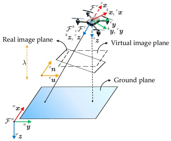
Two coordinate frames are considered to construct the dynamic model of the quadrotor MAV. As shown in Figure 1, the world frame ${\mathcal{F}}^w$ is defined with its origin fixed on the ground, with directions of north–east–down. The body frame ${\mathcal{F}}^b$ is attached to the MAV with its origin located at the center of mass and oriented in the forward–right–down directions. Its position and attitude with respect to ${\mathcal{F}}^w$ are denoted by $\mathit{\xi }(t)=[x(t),y(t),$ $z(t){]}^T$ and a rotation matrix $R(t)$, respectively. $R(t)$ is associated with the attitude of three Euler angles, $\phi (t)$, $\theta (t)$, and $\psi (t)$, which indicate the roll, pitch, and yaw angles, respectively.

Figure 1. Coordinate frames and geometric relationship of an MAV during IBVS.

Following [25], the dynamic equations of the quadrotor MAV are expressed as:

$$\dot{\mathit{\xi }}=R\mathit{v},$$

(1)

$$\dot{R}=R\mathrm{sk}(\mathit{\omega }),$$

(2)

$$m\dot{\mathit{v}}=-m\mathit{\omega }\times \mathit{v}+\mathit{F},$$

(3)

$$J\dot{\mathit{\omega }}=-\mathit{\omega }\times J\mathit{\omega }+\mathit{\tau },$$

(4)

$$\mathit{F}=-U{\mathit{e}}_3+mg{R}^T{\mathit{e}}_3$$

(5)

where $\mathit{v}(t)={[v_x(t),v_y(t),v_z(t)]}^T$ and $\mathit{\omega }(t)={[{\omega }_x(t),{\omega }_y(t),{\omega }_z(t)]}^T$ represent the linear velocity and angular velocity of the MAV expressed under ${\mathcal{F}}^b$, respectively. $m$ and $g$ denote the mass of the MAV and the gravitational acceleration, respectively. $\mathit{F}(t)\in {\mathbb{R}}^3$ is the force vector along the $\mathit{z}$-axis of ${\mathcal{F}}^b$, and $J\in {\mathbb{R}}^{3\times 3}$ is the MAV inertia matrix. $\mathit{\tau }\in {\mathbb{R}}^3$ and $U(t)$ denote the torque vector and total thrust vector of the MAV expressed under ${\mathcal{F}}^b$, respectively. ${\mathit{e}}_3={[0,0,1]}^T$ represents a unit vector along the vertical axis. $\times$ and $\mathrm{sk}(\cdot )$ represent the cross product and antisymmetric matrix, respectively.

2.2. Image Feature Dynamics

As illustrated in Figure 1, a virtual camera frame is introduced to provide decoupled image dynamics for the lateral motion of the MAV. The origin of the camera frame ${\mathcal{F}}^c$ is aligned with the projection center of the downward camera, assuming that ${\mathcal{F}}^c$ coincides with ${\mathcal{F}}^b$. By rotating ${\mathcal{F}}^c$ to align ${}^{c}z$ with ${}^{w}z$, we obtain the virtual camera frame ${\mathcal{F}}^v$, which shares the same origin as ${\mathcal{F}}^c$, has the same yaw angle, and maintains zero roll and pitch angles relative to ${\mathcal{F}}^w$. Consequently, projecting feature points onto a virtual image plane parallel to the horizontal plane eliminates the effects from the MAV’s roll and pitch motions, thus achieving decoupled image dynamics.

Consider a fixed point denoted under ${\mathcal{F}}^w$ and ${\mathcal{F}}^v$ as ${}^w\mathit{p}(t)={[{}^{w}x(t),{}^{w}y(t),{}^{w}z(t)]}^T$ and ${}^v\mathit{p}(t)={[{}^{v}x(t),{}^{v}y(t),{}^{v}z(t)]}^T$, respectively. By transforming the frame, the following relationship can be obtained:

$${}^v\mathit{p}=R_{\psi }^T({}^w\mathit{p}-{}^w\mathit{T}_v),$$

(6)

$${}^v\dot{\mathit{p}}=-\mathrm{sk}(\dot{\psi }{\mathit{e}}_3){}^v\mathit{p}-{}^v\mathit{v}$$

(7)

where $R_{\psi }(t)$ is the yaw rotation matrix of ${\mathcal{F}}^v$ under ${\mathcal{F}}^w$, ${}^w\mathit{T}_v\in {\mathbb{R}}^3$ is the position of ${\mathcal{F}}^v$ relative to ${\mathcal{F}}^w$, and ${}^v\mathit{v}(t)={[{}^{v}v_x(t),{}^{v}v_y(t),{}^{v}v_z(t)]}^T$ is the linear velocity of the MAV expressed under ${\mathcal{F}}^v$.

The camera’s focal length is $\lambda >0$. According to the perspective projection model, the pixel coordinate ${[{}^{v}u(t),{}^{v}n(t)]}^T$ of ${}^v\mathit{p}(t)$ in the virtual image plane and the mapping relationship between ${}^v\mathit{p}(t)$ and ${}^v\mathit{v}(t)$ are as follows:

$$\left[\begin{array}{c}{}^{v}u\\ {}^{v}n\end{array}\right]={\displaystyle \frac{\lambda }{{}^{v}z}}\left[\begin{array}{c}{}^{v}x\\ {}^{v}y\end{array}\right],$$

(8)

$$\left[\begin{array}{c}{}^v\dot{u}\\ {}^v\dot{n}\end{array}\right]=\left[\begin{array}{ccc}-\lambda {/}^{v}z& 0& {}^{v}u{/}^{v}z\\ 0& -\lambda {/}^{v}z& {}^{v}n{/}^{v}z\end{array}\right]\left[\begin{array}{c}{}^{v}v_x\\ {}^{v}v_y\\ {}^{v}v_z\end{array}\right]+\left[\begin{array}{c}{}^{v}n\\ {-}^{v}u\end{array}\right]\dot{\psi }.$$

(9)

Consider $N$ stationary feature points projected from a horizontal target plane onto the virtual image plane; the center coordinates ${[{}^{v}u_g,{}^{v}n_g]}^T$ of the target plane are

$${}^{v}u_g={\displaystyle \frac{1}{N}}{\displaystyle \sum _{k=1}^N{}^{v}u_k}, {}^{v}n_g={\displaystyle \frac{1}{N}}{\displaystyle \sum _{k=1}^N{}^{v}n_k}.$$

(10)

Then, image moments $\mathit{q}(t)={[q_x(t),q_y(t),q_z(t)]}^T$ and $q_{\psi }$ are selected to control the translation and rotation of the MAV, respectively [25].

$$q_x=q_z{\displaystyle \frac{{}^{v}u_g}{\lambda }}, q_y=q_z{\displaystyle \frac{{}^{v}n_g}{\lambda }}, q_z=\sqrt{{\displaystyle \frac{a^{\ast }}{a}}}, q_{\psi }={\displaystyle \frac{1}{2}}\arctan {\displaystyle \frac{2{}^v\mu _{11}}{{}^v\mu _{20}-{}^v\mu _{02}}}$$

(11)

where ${}^v\mu _{\mathit{ij}}={\displaystyle {\sum }_{k=1}^N{({}^{v}u_k-{}^{v}u_g)}^i{({}^{v}n_k-{}^{v}n_g)}^j}$, $a={}^v\mu _{20}+{}^v\mu _{02}$ represents the pixel region of the visual target with ${}^{v}z\sqrt{a}=z^{\ast }\sqrt{a^{\ast }}$. ${}^{v}z(t)={}^{w}z(t)$ is the vertical distance of the target relative to the camera, and $a^{\ast }$ and $z^{\ast }$ represent the values of $a(t)$ and ${}^{v}z(t)$ when the MAV reaches the desired pose.

The image moment dynamics can be obtained by combining Equations (9) and (11) as follows:

$$\dot{\mathit{q}}=-\mathrm{sk}(\dot{\psi }{\mathit{e}}_3)\mathit{q}-{\displaystyle \frac{1}{z^{\ast }}}{}^v\mathit{v},$$

(12)

$${\dot{q}}_{\psi }=-\dot{\psi }.$$

(13)

3. Observer Design

To address the issue that onboard sensors cannot continuously provide linear velocity information for the MAV during IBVS tasks, an approximate observation method [40] is introduced in this section, and a linear velocity observer with high accuracy and fast convergence is designed on the basis of this method.

First, we express the translational dynamics (4) and (5) of the MAV under ${\mathcal{F}}^v$:

$${}^v\dot{\mathit{v}}=-\mathrm{sk}(\dot{\psi }{\mathit{e}}_3){}^v\mathit{v}+\mathit{f},$$

(14)

$$\mathit{f}={\displaystyle \frac{-R_{\phi \theta }U{\mathit{e}}_3}{m}}+g{\mathit{e}}_3$$

(15)

where $\mathit{f}(t)={[f_x(t),f_y(t),f_z(t)]}^T$ is the total force for the MAV under ${\mathcal{F}}^v$, $R_{\phi \theta }(t)$ is the rotation matrix of ${\mathcal{F}}^b$ relative to ${\mathcal{F}}^v$, which successively rotates in the roll and pitch directions. The dynamics are consistent with the nonlinear multi-input multi-output system discussed in [40], and, therefore, the approximate observation method can be applied to the translational dynamics of the MAV.

The auxiliary correction terms $\mathit{\zeta }(t)={[{\zeta }_x(t),{\zeta }_y(t),{\zeta }_z(t)]}^T=\widehat{\mathit{q}}(t)$ and $\mathit{\delta }(t)=[{\delta }_x(t),$${\delta }_y(t),{\delta }_z(t){]}^T=\widehat{\dot{\mathit{q}}}(t)$ are defined to observe $\mathit{q}(t)$ and $\dot{\mathit{q}}(t)$, respectively. Let ${}^v\widehat{\mathit{v}}(t)$ denote the observed value of ${}^v\mathit{v}(t)$. Then, according to (12), ${}^v\widehat{\mathit{v}}(t)$ can be obtained from $\mathit{\zeta }(t)$ and $\mathit{\delta }(t)$ as follows:

$${}^v\widehat{\mathit{v}}=-z^{\ast }\mathit{\delta }-z^{\ast }\mathrm{sk}(\dot{\psi }{\mathit{e}}_3)\mathit{\zeta }.$$

(16)

Subsequently, based on the approximate observation method in [40], the following observer is designed to estimate the linear velocity of the MAV:

$$\dot{\mathit{\zeta }}=-\mathrm{blkdiag}({\displaystyle \frac{{\eta }_1}{\alpha }},{\displaystyle \frac{{\eta }_2}{\alpha }},{\displaystyle \frac{{\eta }_3}{\alpha }})\mathit{\zeta }+\mathrm{blkdiag}({\displaystyle \frac{{\eta }_1}{\alpha }},{\displaystyle \frac{{\eta }_2}{\alpha }},{\displaystyle \frac{{\eta }_3}{\alpha }})\mathit{q}+\mathit{\delta },$$

(17)

$$\dot{\mathit{\delta }}=-\mathrm{blkdiag}({\displaystyle \frac{{\epsilon }_1}{\alpha ^2}},{\displaystyle \frac{{\epsilon }_2}{\alpha ^2}},{\displaystyle \frac{{\epsilon }_3}{\alpha ^2}})\mathit{\zeta }+\mathrm{blkdiag}({\displaystyle \frac{{\epsilon }_1}{\alpha ^2}},{\displaystyle \frac{{\epsilon }_2}{\alpha ^2}},{\displaystyle \frac{{\epsilon }_3}{\alpha ^2}})\mathit{q}+{\displaystyle \frac{\partial \mathit{\delta }}{\partial \mathit{\zeta }}}{\displaystyle \frac{\partial \mathit{\zeta }}{\partial t}},$$

(18)

$${}^v\widehat{\mathit{v}}=\mathrm{blkdiag}({\rho }_1,{\rho }_2,{\rho }_3)[-z^{\ast }\mathit{\delta }-z^{\ast }\mathrm{sk}(\dot{\psi }{\mathit{e}}_3)\mathit{\zeta }],$$

(19)

$${\rho }_i=(1-{\displaystyle \frac{1}{{\displaystyle \sum dt}}})^\left[{\displaystyle \frac{{}^i\rho _1}{({\displaystyle \sum dt})^{}^i\rho _2}}\right], i=1, 2, 3$$

(20)

where $\mathrm{blkdiag}(\cdot )$ denotes the diagonalization of the matrix or values within the parentheses. For $i=1, 2, 3$, the observation gains ${\eta }_i$, ${\epsilon }_i$, and $\alpha$ are positive constants, ensuring the observation gain matrices are positive definite. Moreover, $\alpha$ must be sufficiently small to achieve precise observation performance. $dt$ represents the time of the control sampling period, while ${\displaystyle \sum dt}=t$ denotes the total time of the current velocity observation. The symbol $^(\cdot )$ indicates the exponentiation operation on the value inside the parentheses.

Remark 1. 

From the perspectives of the observer dynamics structure, the error convergence mechanism, and the design principle of rapid convergence dominated by the gain parameter $\alpha$, the observer designed in this article, based on the approximate observation method [40], falls into the category of high-gain observers discussed in [41,42]. In [42], the approximate observation method of [40] was further developed into a complete high-gain observer theory, and a proof of semi-global practical asymptotic stability (SGPAS) was provided. Within this observer framework, the observed values inherently exhibit a peaking phenomenon at the initial moment, which is not guaranteed to be uniformly bounded in a global sense. To address this inherent characteristic, an approximate transition term ${\rho }_i$ is designed in (20) to eliminate the undesirable behavior of the observed values at the initial moment.

To ensure rapid convergence from a large initial error, an approximate transition term ${\rho }_i$ is designed, where ${}^i\rho _1$ and ${}^i\rho _2$ are positive constants, and ${}^i\rho _1$ must be sufficiently large to optimize the initial phase of approximate observation. This design makes the observed results align more closely with the actual values, thereby enabling the provision of reliable state information for the MPC controller.

4. Model Predictive Control

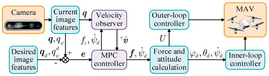
The control objective is to efficiently compute the optimal control inputs based on the image moments in order to adjust the MAV’s attitude and position. The overall control scheme is illustrated in Figure 2.

Figure 2. The block diagram of the control scheme.

The expected image moments ${\mathit{q}}_d(t)$ and $q_{\psi }^d(t)$ and the image feature error $\mathit{e}(t)$ are defined as:

$${[{\mathit{q}}_d,q_{\psi }^d]}^T={[q_x^d,q_y^d,q_z^d,q_{\psi }^d]}^T={[0,0,1,0]}^T,$$

(21)

$$\mathit{e}(t)={[\mathit{q},q_{\psi }]}^T-{[{\mathit{q}}_d,q_{\psi }^d]}^T={[e_x,e_y,e_z,e_{\psi }]}^T.$$

(22)

The dynamics of the image feature error can be expressed as:

$${\dot{e}}_x=\dot{\psi }{e}_y-{\displaystyle \frac{1}{z^{\ast }}}{}^{v}v_x, {\dot{e}}_y=-\dot{\psi }{e}_x-{\displaystyle \frac{1}{z^{\ast }}}{}^{v}v_y, {\dot{e}}_z=-{\displaystyle \frac{1}{z^{\ast }}}{}^{v}v_z, {\dot{e}}_{\psi }=-\dot{\psi }.$$

(23)

When the MAV is in the desired pose, $\mathit{e}(t)=0$ and ${}^v\mathit{v}(t)=0$. Therefore, in the system $\dot{\mathbf{x}}=F(\mathbf{x},\mathbf{u})$, the system state is defined as $\mathbf{x}(t)={[{\mathit{e}}^T(t),{}^v\mathit{v}^T(t)]}^T$, and the control input is selected as $\mathbf{u}(t)={[{\mathit{f}}^T(t),\dot{\psi }(t)]}^T$. The control objective is formulated as the rapid convergence of the system to the zero equilibrium points ${\mathbf{x}}_d(t)$ and ${\mathbf{u}}_d(t)$. The ultimate control objective is $\mathbf{x}(t)={\mathbf{x}}_d(t)=0$, $\mathbf{u}(t)={\mathbf{u}}_d(t)=0$. During IBVS task execution, ${}^v\mathit{v}(t)$ is provided by its observed value ${}^v\widehat{\mathit{v}}(t)$.

Let the system state be denoted by $\mathbf{x}(t)={[{\mathbf{x}}_1(t),{\mathbf{x}}_2(t),{\mathbf{x}}_3(t),{\mathbf{x}}_4(t),{\mathbf{x}}_5(t),{\mathbf{x}}_6(t),{\mathbf{x}}_7(t)]}^T$ and the control input be denoted as $\mathbf{u}(t)={[{\mathbf{u}}_1(t),{\mathbf{u}}_2(t),{\mathbf{u}}_3(t),{\mathbf{u}}_4(t)]}^T$. The nonlinear dynamic model of the system can be expressed as:

$$\begin{array}{cc}\dot{\mathbf{x}}& =F(\mathbf{x},\mathbf{u})\hfill \\ & ={[{\mathbf{x}}_2{\mathbf{u}}_4-{\displaystyle \frac{{\mathbf{x}}_5}{z^{\ast }}},-{\mathbf{x}}_1{\mathbf{u}}_4-{\displaystyle \frac{{\mathbf{x}}_6}{z^{\ast }}},-{\displaystyle \frac{{\mathbf{x}}_7}{z^{\ast }}},-{\mathbf{u}}_4,{\mathbf{x}}_6{\mathbf{u}}_4+{\mathbf{u}}_1,-{\mathbf{x}}_5{\mathbf{u}}_4+{\mathbf{u}}_2,{\mathbf{u}}_3]}^T.\hfill \end{array}$$

(24)

During IBVS task execution, the MAV performs small-angle attitude adjustments. With decoupling of image dynamics achieved, the nonlinearities in the MAV dynamics under ${\mathcal{F}}^v$ are solely induced by minor yaw angle variations, resulting in a relatively weak level of system nonlinearity. Therefore, to achieve real-time, efficient, and low-computational-cost control performance, the focus is placed on approximating the system as linear and constructing an MPC controller based on this approximation.

We decompose the nonlinear term by a first-order Taylor expansion of $F(\mathbf{x},\mathbf{u})$ at the zero equilibrium points and realize the linearization approximation of the system.

$$F(\mathbf{x},\mathbf{u})\approx F({\mathbf{x}}_d,{\mathbf{u}}_d)+{\displaystyle \frac{\partial F}{\partial \mathbf{x}}}\left|{}_{({\mathbf{x}}_d,{\mathbf{u}}_d)}(\mathbf{x}-{\mathbf{x}}_d)\right.+{\displaystyle \frac{\partial F}{\partial \mathbf{u}}}\left|{}_{({\mathbf{x}}_d,{\mathbf{u}}_d)}(\mathbf{u}-{\mathbf{u}}_d)\right..$$

(25)

Subsequently, the linear discrete-time system can be obtained:

$$\mathbf{x}(k+1)=A\mathbf{x}(k)+B\mathbf{u}(k)$$

(26)

where $k$ denotes the discrete sampling instant and $\mathbf{x}(k)$ and $\mathbf{u}(k)$ represent the system state and control input at each sampling instant in a linear discrete system, respectively. The fully known state matrix $A$ and input matrix $B$ are given by:

$$A=\left[\begin{array}{ccccccc}1& 0& 0& 0& {\displaystyle \frac{-dt}{z^{\ast }}}& 0& 0\\ 0& 1& 0& 0& 0& {\displaystyle \frac{-dt}{z^{\ast }}}& 0\\ 0& 0& 1& 0& 0& 0& {\displaystyle \frac{-dt}{z^{\ast }}}\\ 0& 0& 0& 1& 0& 0& 0\\ 0& 0& 0& 0& 1& 0& 0\\ 0& 0& 0& 0& 0& 1& 0\\ 0& 0& 0& 0& 0& 0& 1\end{array}\right], B=\left[\begin{array}{cccc}0& 0& 0& 0\\ 0& 0& 0& 0\\ 0& 0& 0& 0\\ 0& 0& 0& -dt\\ -dt& 0& 0& 0\\ 0& -dt& 0& 0\\ 0& 0& -dt& 0\end{array}\right].$$

(27)

The linearization approximation error $\mathrm{\Delta }(t)$ of the system can be expressed as:

$$\mathrm{\Delta }={\displaystyle \frac{‖\mathbf{x}(k)+F(\mathbf{x},\mathbf{u})dt-A\mathbf{x}(k)-B\mathbf{u}(k)‖}{‖F(\mathbf{x},\mathbf{u})dt‖}}.$$

(28)

Remark 2. 

For flight systems requiring high real-time performance and high control frequency, we employ high-speed sampling to enable intensive discrete control of continuous systems while updating the system state in real time, thereby eliminating errors accumulated from rolling optimization based on the linearized dynamics. At each control cycle, the state information is updated for the controller based on the image moment error $\mathit{e}(t)$ and the velocity observed value ${}^v\widehat{\mathit{v}}(t)$. Furthermore, subsequent simulation results verify that the linearization approximation error $\mathrm{\Delta }(t)$ can be strictly confined within 4%. Meanwhile, the state update mechanism effectively suppresses errors accumulated during the processes of linear approximation and rolling optimization, thereby ensuring the steady-state accuracy of the system.

Next, an MPC approach [37] is designed for this linear discrete-time system. First, the prediction model for the system state is formulated as follows:

$$\mathbf{x}(k+i+1\left|k\right.)=A\mathbf{x}(k+i\left|k\right.)+B\mathbf{u}(k+i\left|k\right.), i=1, 2, \cdots , N-1$$

(29)

where $i$ and $N$ represent the prediction step and the prediction horizon, respectively. The predicted system state for each control cycle can be compactly expressed as:

$$\mathbf{X}(k)=M\mathbf{x}(k)+C\mathbf{U}(k)$$

(30)

where $\mathbf{X}(k)$ and $\mathbf{U}(k)$ denote the prediction sequences of the system state and input, respectively, while $M$ and $C$ are the matrices associated with $A$ and $B$, as expressed in the following forms:

$$\mathbf{X}(k)={[\mathbf{x}(k\left|k\right.), \mathbf{x}(k+1\left|k\right.), \cdots , \mathbf{x}(k+N\left|k\right.)]}^T,$$

(31)

$$\mathbf{U}(k)={[\mathbf{u}(k\left|k\right.), \mathbf{u}(k+1\left|k\right.), \cdots , \mathbf{u}(k+N-1\left|k\right.)]}^T,$$

(32)

$$M={[I, A^T, {(A^2)}^T, \cdots , {(A^N)}^T]}^T,$$

(33)

$$C=\left[\begin{array}{cccc}O& \cdots & & O\\ B& O& \cdots & O\\ \mathit{AB}& B& \cdots & O\\ ⋮& & & ⋮\\ A^(N-1)B& A^(N-2)B& \cdots & B\end{array}\right].$$

(34)

Subsequently, by employing the positive definite weight matrices $Q$, $R$ and $Q_f$, we define the following cost function for rolling optimization of three performance metrics: system state error, feasible range of input consumption, and closed-loop stability of the system terminal.

$$\begin{array}{cc}J(k)& ={\displaystyle \sum _{i=0}^{N-1}[\mathbf{x}{(k+i\left|k\right.)}^{T}Q\mathbf{x}(k+i\left|k\right.)+\mathbf{u}{(k+i\left|k\right.)}^{T}R\mathbf{u}(k+i\left|k\right.)]}\hfill \\ & +\mathbf{x}{(k+N\left|k\right.)}^T{Q}_f\mathbf{x}(k+N\left|k\right.)\hfill \\ & =\mathbf{X}(k)\overline{Q}\mathbf{X}{(k)}^T+\mathbf{U}(k)\overline{R}\mathbf{U}{(k)}^T\hfill \end{array}$$

(35)

where $\overline{Q}=\mathrm{blkdiag}(Q,Q,\cdots ,Q,Q_f)$ and $\overline{R}=\mathrm{blkdiag}(R,R,\cdots ,R)$. By updating the system state and solving the optimization problem of the cost function at each control cycle, the optimal control sequence ${\mathbf{U}}^{\ast }(k)$ and the control input $\mathbf{u}(k)$ for the corresponding discrete time step can be obtained.

$${\mathbf{U}}^{\ast }(k)=\underset{\mathbf{U}(k)}{\min }[J(k)],$$

(36)

$$\mathbf{u}(k)=\left[\begin{array}{cccc}1& 0& \cdots & 0\end{array}\right]{\mathbf{U}}^{\ast }(k).$$

(37)

According to (15), the thrust and attitude inputs required by the MAV can be calculated as follows:

$$\mathbf{f}=\left[\begin{array}{cccc}1& 0& 0& 0\\ 0& 1& 0& 0\\ 0& 0& 1& 0\end{array}\right]\mathbf{u},$$

(38)

$$U=m{e}_3^T{R}_{\phi \theta }^T(g{e}_3-f),$$

(39)

$${\phi }_d=\arctan {\displaystyle \frac{-f_y\cos {\theta }_d}{f_z-g}},$$

(40)

$${\theta }_d=\arctan {\displaystyle \frac{f_x}{f_z-g}},$$

(41)

$${\dot{\psi }}_d=\left[\begin{array}{cccc}0& 0& 0& 1\end{array}\right]\mathbf{u}.$$

(42)

For the autonomous flight of MAVs, a mature control design adopts a dual-loop architecture, in which the inner-loop attitude control operates at a higher frequency than the outer-loop position control. Regarding the proposed control strategy, $U(k)$ is input to the outer-loop controller, and ${\phi }_d(k)$, ${\theta }_d(k)$, and ${\dot{\psi }}_d(k)$ are input to the inner-loop controller, thereby enabling the MAV to accomplish the IBVS task.

5. Simulation Results

In this section, two distinct types of experiments are conducted. First, a simulation test is performed using a horizontal target plane with four points, and a comparison is made with the classical backstepping-based IBVS control method [21], thereby validating the performance of the proposed velocity observer and the MPC controller in IBVS tasks. Subsequently, the feasibility of the linearization approximation is verified through another simulation test, taking into account the influence of the maximum nonlinear coupling terms.

5.1. Simulation Results Compared with the Backstepping-Based Method

Simulation tests are conducted in MATLAB R2020b with a sampling period $dt$ of $0.01 \mathrm{s}$. The MAV mass is set as $m=2 \mathrm{kg}$, gravitational acceleration is $g=9.81{ \mathrm{m}/\mathrm{s}}^2$, and the camera focal length is $\lambda =1.8 \mathrm{mm}$. It is assumed that target points are already in the camera field of view (FOV). The coordinates of four target points under ${\mathcal{F}}^w$ are ${[0.25,0.5,0]}^T\mathrm{m}$, ${[-0.25,0.5,0]}^T\mathrm{m}$, ${[-0.25,-0.5,0]}^T\mathrm{m}$, and ${[0.25,-0.5,0]}^T\mathrm{m}$. The MAV is hovering at the initial moment with the Euler angles $\phi (t)=\theta (t)=0 \mathrm{rad}$ and $\psi (t)=0.174 \mathrm{rad}$ under ${\mathcal{F}}^w$ and with the position ${[3,2,-8]}^T\mathrm{m}$ under ${\mathcal{F}}^w$.

The desired position and Euler angles of the MAV under ${\mathcal{F}}^w$ are set as ${[0,0,-4]}^T\mathrm{m}$ and ${[0,0,0]}^T\mathrm{rad}$, respectively, with the parameter $a^{\ast }=2.5\times {10}^{-7}$. Observer gains are chosen as ${\eta }_i=15$, ${\epsilon }_i=15$, and $\alpha =0.1$. ${}^1\rho _1$, ${}^2\rho _1$, ${}^3\rho _1$, ${}^1\rho _2$, ${}^2\rho _2$, and ${}^3\rho _2$ are chosen as $1.2\times {10}^4$, $1.2\times {10}^4$, $1.5\times {10}^4$, $1.2$, $1.2$, and $1.5$, respectively. Control weight matrices $Q$, $R$, $Q_f$ are set as $\mathrm{blkdiag}(1500,1500,1500,5,8,8,8)$, $\mathrm{blkdiag}(0.5,0.5,0.5,0.5)$, and $\mathrm{blkdiag}(1300,1300,1300,3,8,8,8)$, respectively. In the simulation test, the dynamic response characteristics and steady-state accuracy are intuitively evaluated through the response curves of the system state $\mathbf{x}(k)$ and control input $\mathbf{u}(k)$.

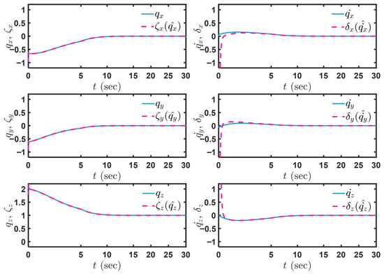
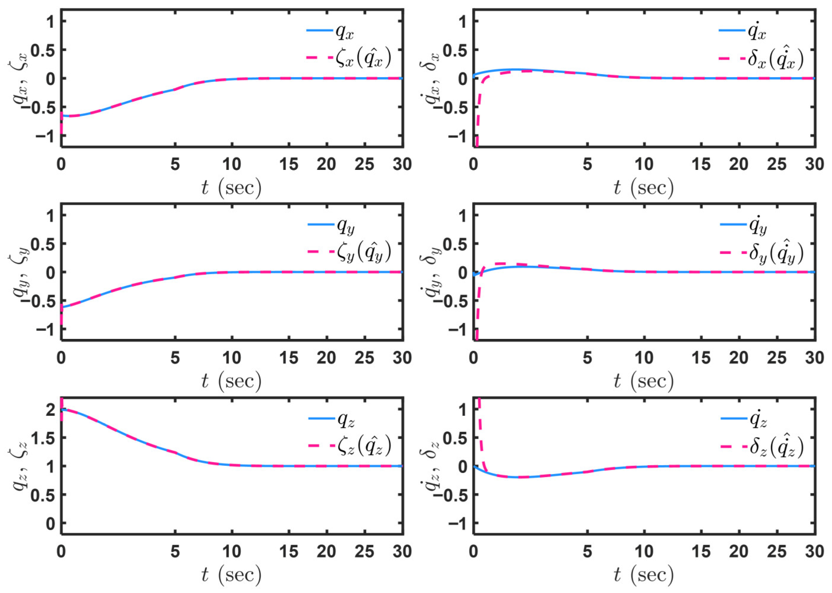
Figure 3 presents the response curves of the auxiliary correction terms $\mathit{\zeta }(t)$ and $\mathit{\delta }(t)$. To more clearly illustrate the dynamic convergence process of the observed values, the time axis in the initial phase is locally magnified. As shown in Figure 3, the auxiliary correction terms converge asymptotically and rapidly to their true values and maintain stable tracking. This result demonstrates that the nonlinear observer designed based on the auxiliary correction terms is capable of obtaining high-precision and high-reliability velocity observations, thereby providing accurate state feedback for the MPC controller.

Figure 3. Simulation results: Evolution of auxiliary correction terms $\mathit{\zeta }(t)$ and $\mathit{\delta }(t)$.

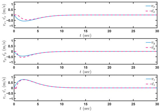
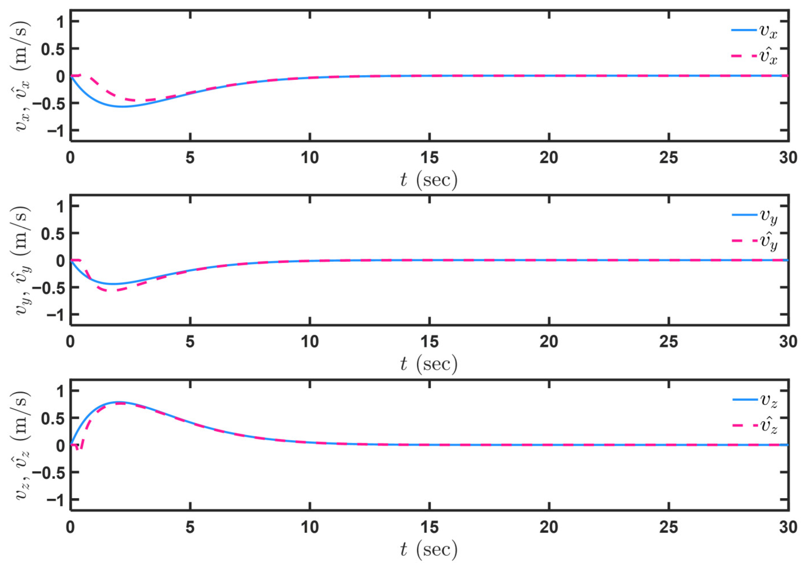
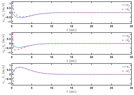
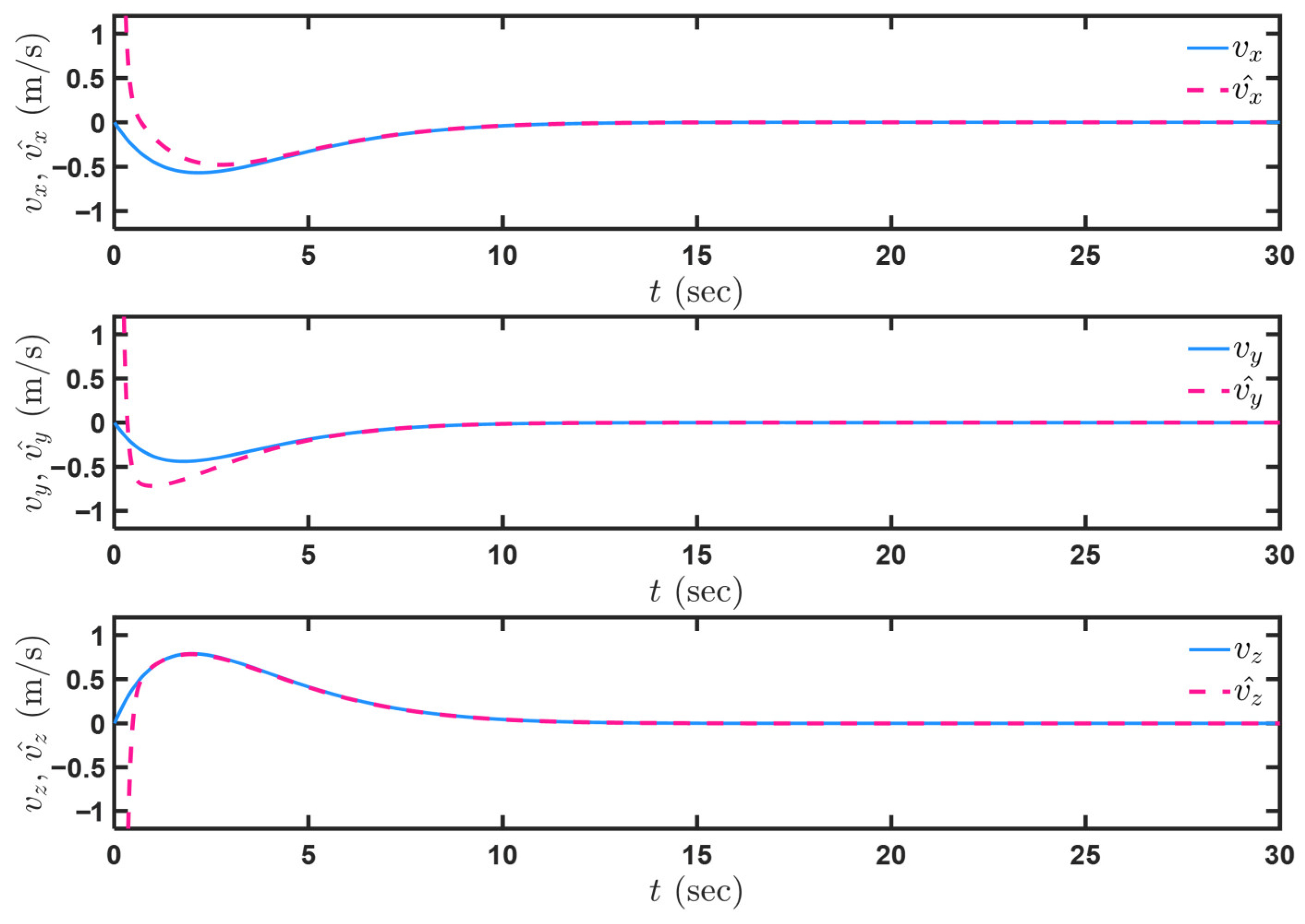
The results of velocity observation are presented in Figure 4. To facilitate comparison with the linear velocity $\mathit{v}(t)$ of the MAV expressed in ${\mathcal{F}}^b$, the observed value $\widehat{\mathit{v}}(t)=[{\widehat{v}}_x(t),$${\widehat{v}}_y(t),$${\widehat{v}}_z(t){]}^T$ of $\mathit{v}(t)$ can be obtained via the following transformation:

$$\widehat{\mathit{v}}=R_{\phi \theta }^T {}^v\widehat{\mathit{v}}.$$

(43)

Figure 4. Simulation results (approximate transition term introduced): Observation for MAV velocities.

Furthermore, in comparison with Figure 5, it can be observed that the introduced approximate transition term ${\rho }_i$ optimizes the infinite asymptotic behavior in the initial phase of the original approximate observation method, resulting in a convergence trajectory that more closely approximates the actual values. This eliminates the infinite velocity observed at the initial moment, facilitating the use of the observed values for system state updates.

Figure 5. Simulation results (approximate transition term not introduced): Observation for MAV velocities.

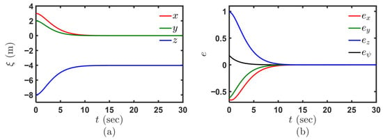
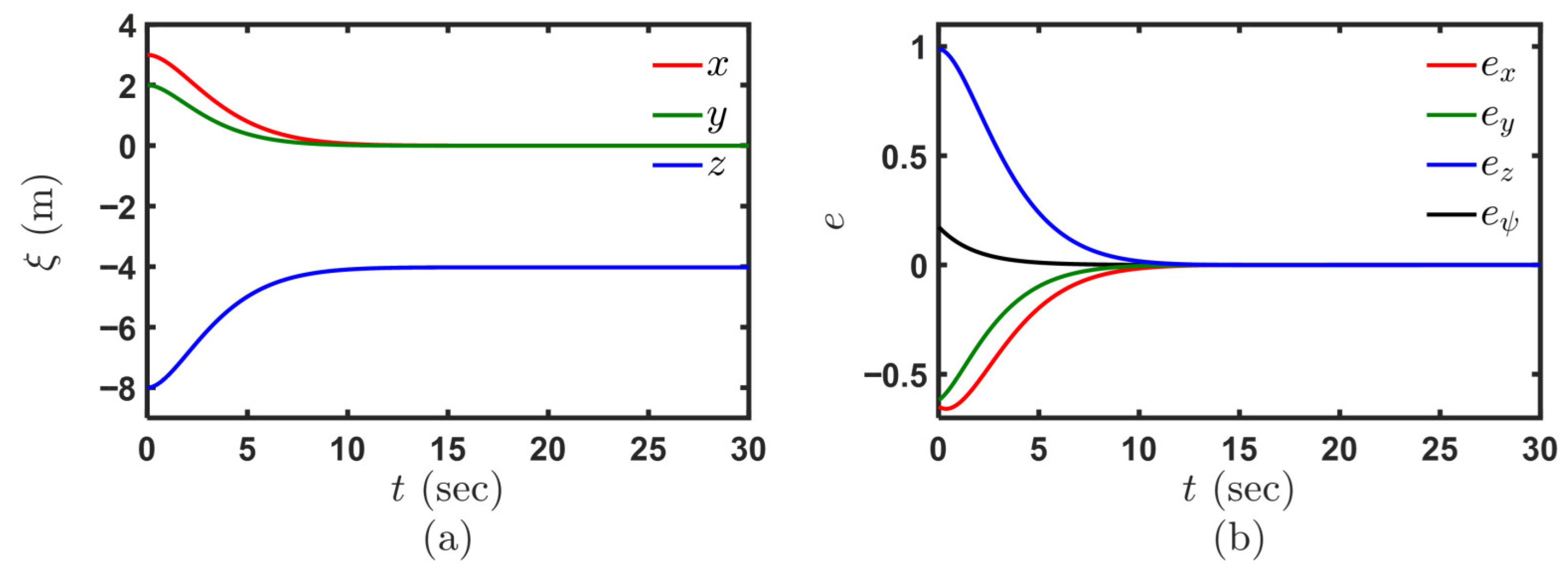
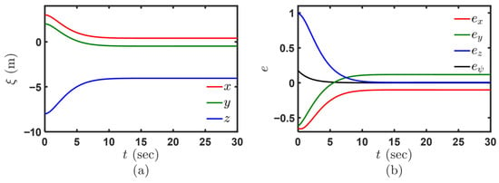
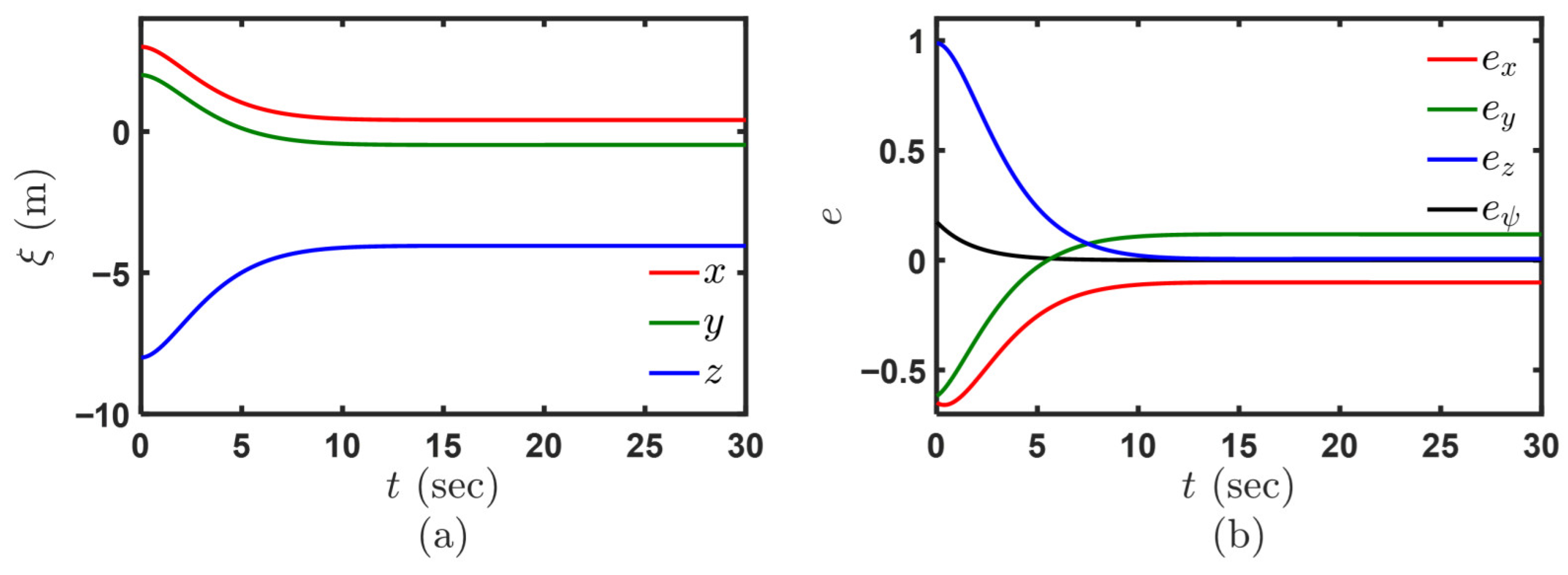
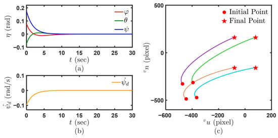
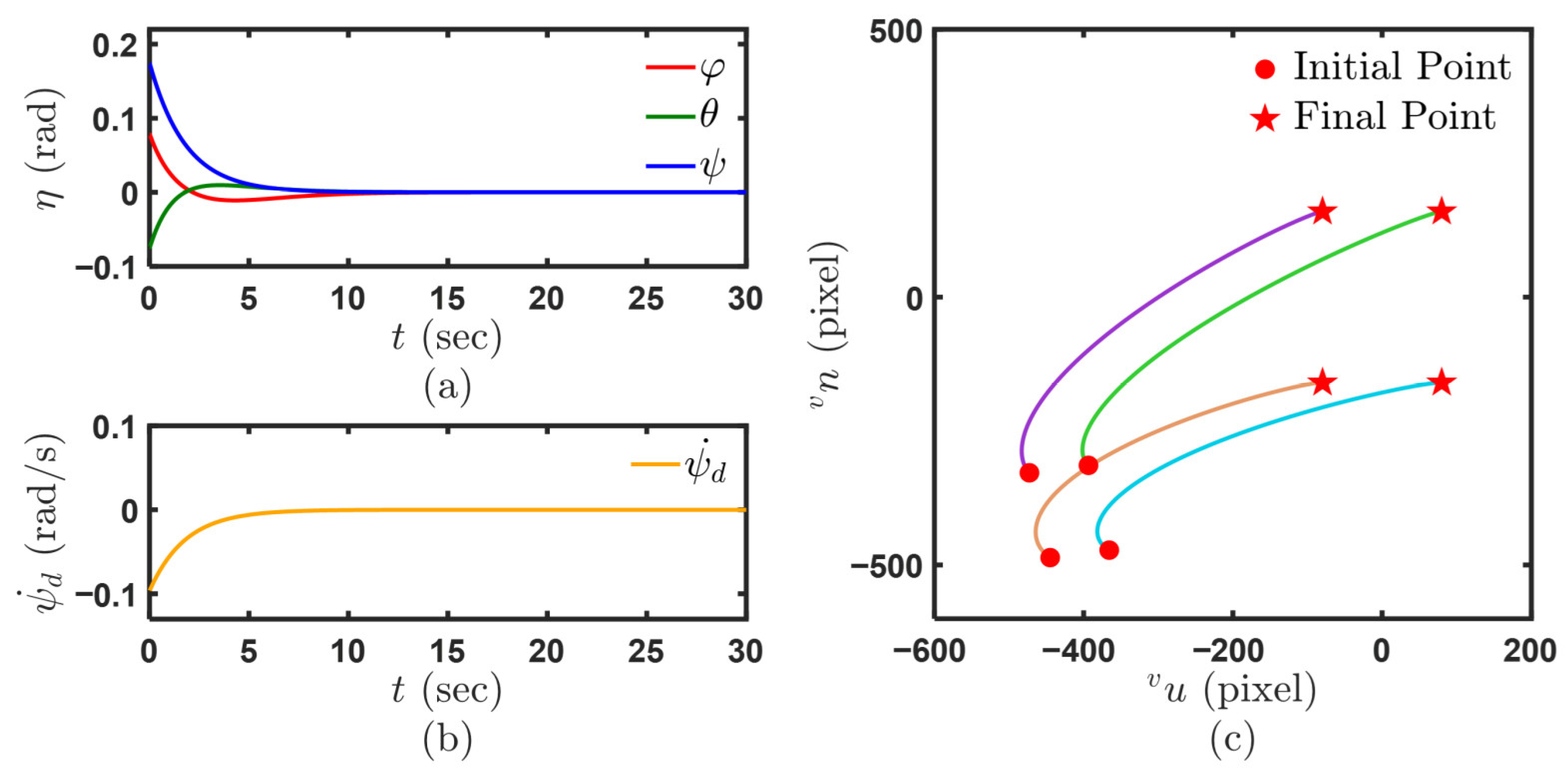
The performance of the proposed control strategy is evaluated in Figure 6, Figure 7 and Figure 8. As shown in Figure 6, the position of the MAV and the image feature error converge rapidly to the desired values. It is noteworthy that the MPC controller is constructed based on a linearly approximated system. Although the influence of the nonlinear terms on the system is relatively weak and the approximation remains highly accurate, the system is fundamentally not an ideal linear one. Consequently, model predictions can accumulate errors due to the influence of nonlinear terms, leading to steady-state errors, as shown in Figure 7. Therefore, it is necessary to update the system state at each control cycle. This update relies on the velocity observer, which uses image feedback to continuously provide the otherwise unavailable linear velocity information. Figure 8 shows that the Euler angles and control input ${\dot{\psi }}_d(k)$ of the MAV converge smoothly and rapidly under the proposed control strategy. Moreover, the trajectories of the target points appear smooth in the virtual image plane. It can be observed that the designed controller demonstrates rapid convergence, enabling the MAV to maintain a stable hover in the desired pose.

Figure 6. Simulation results (system state continuously updated): (a) MAV positions under ${\mathcal{F}}^w$. (b) Image feature error vectors.

Figure 7. Simulation results (system state not updated): (a) MAV positions under ${\mathcal{F}}^w$. (b) Image feature error vectors.

Figure 8. Simulation results: (a) MAV Euler angles. (b) Evolution of ${\dot{\psi }}_d(k)$. (c) Paths of target points in the virtual image plane.

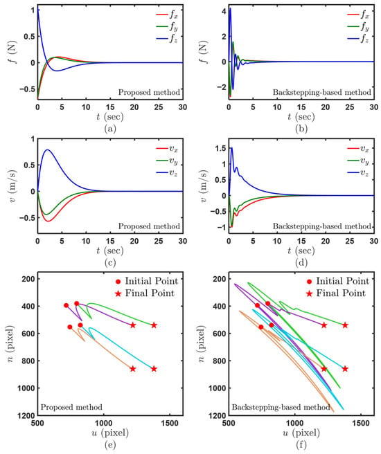
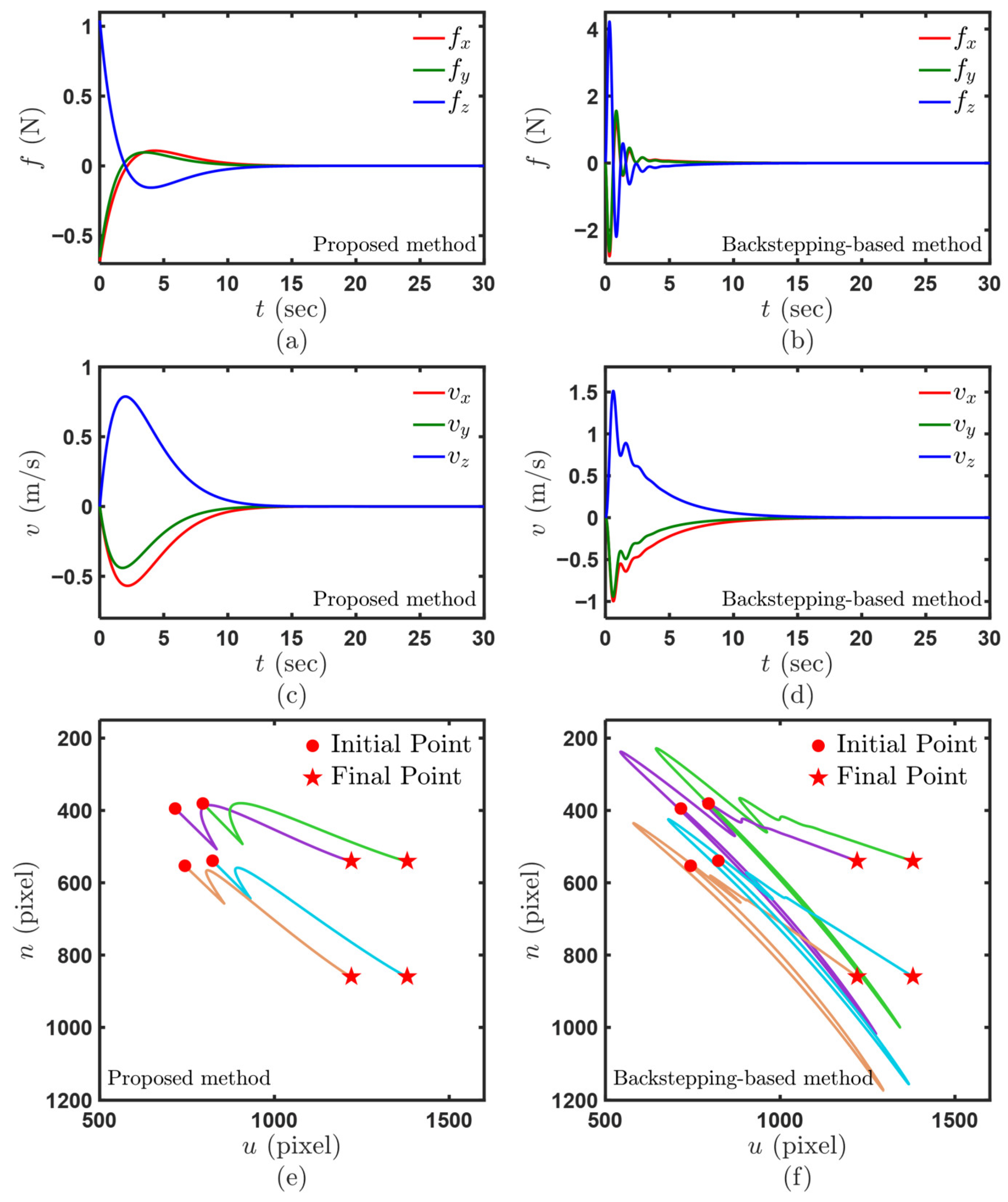
Figure 9 presents the simulation comparison results between the proposed method and the backstepping-based control method. It was verified in [21] that the backstepping-based method can achieve satisfactory image error convergence and precise position regulation in IBVS tasks. Figure 9 further evaluates the advantages of the proposed method in terms of dynamic response through a comparative analysis of velocity, control input and flight trajectory between the two methods. As can be observed from the figure, in contrast to the backstepping-based control method, the proposed MPC control strategy effectively suppresses the aggressive transient responses induced by initial errors by solving for the optimal control input sequence through forward-looking rolling optimization, thereby exhibiting superior dynamic performance in terms of response smoothness.

Figure 9. Simulation results: (a) Force vectors for the MAV (proposed method). (b) Force vectors for the MAV (backstepping-based method). (c) MAV velocities (proposed method). (d) MAV velocities (backstepping-based method). (e) Paths of target points in the real image plane (proposed method). (f) Paths of target points in the real image plane (backstepping-based method).

5.2. Simulation Results Considering the Maximum Nonlinear Coupling Terms

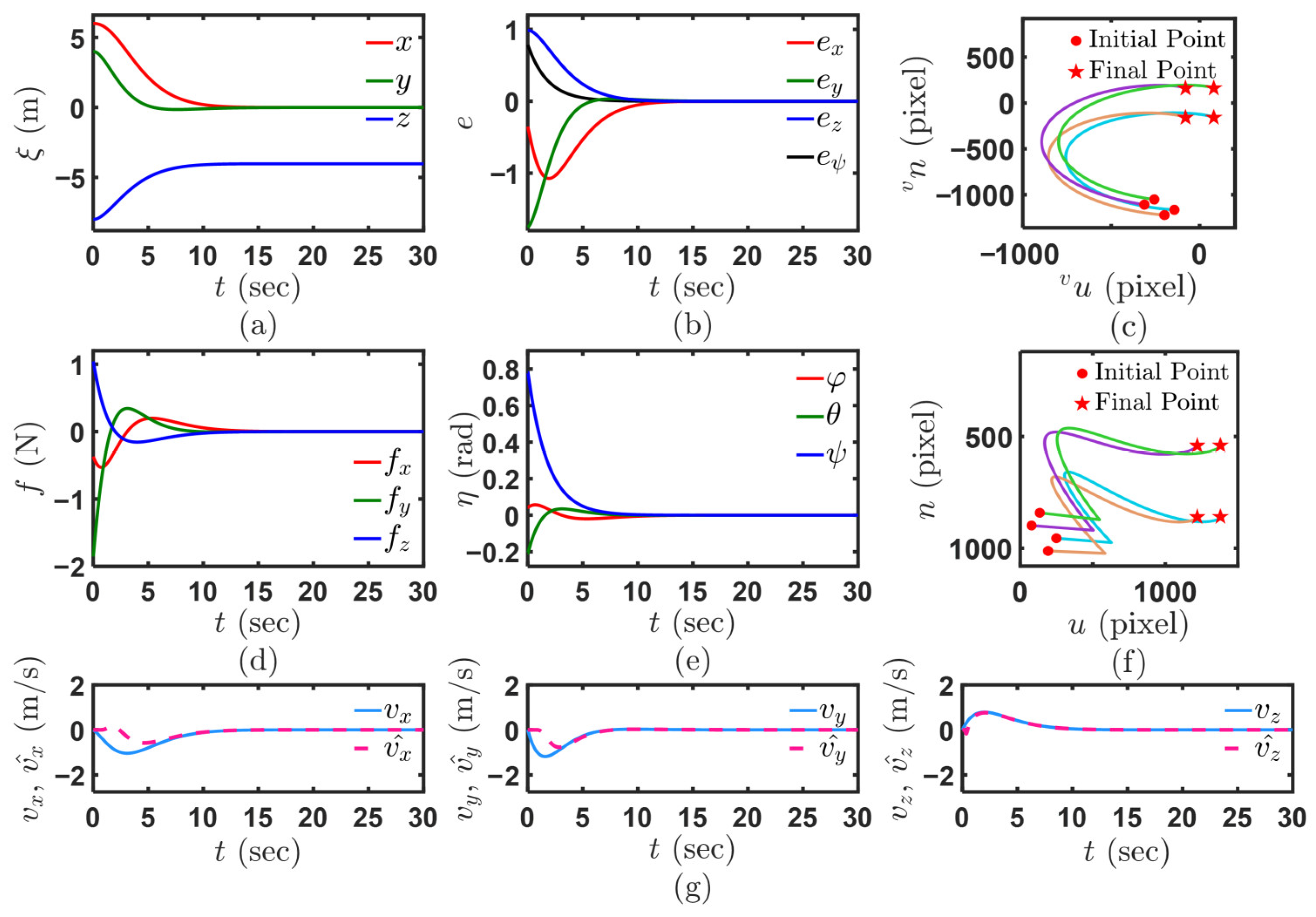
The linearization approximation error consists of coupling terms involving the yaw angle, the image feature error, and the MAV velocity. Therefore, to verify the feasibility of the linearization approximation, a simulation test is conducted under the conditions of maximum yaw angle error and initial image error. Considering the characteristics of image moments and the camera FOV constraints, the initial yaw angle is set to $0.25\pi \mathrm{rad}$ under ${\mathcal{F}}^w$, and the initial position is set to ${[6,4,-8]}^T\mathrm{m}$ under ${\mathcal{F}}^w$. The remaining simulation configurations and parameter settings are kept consistent with the aforementioned simulation tests.

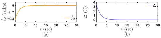
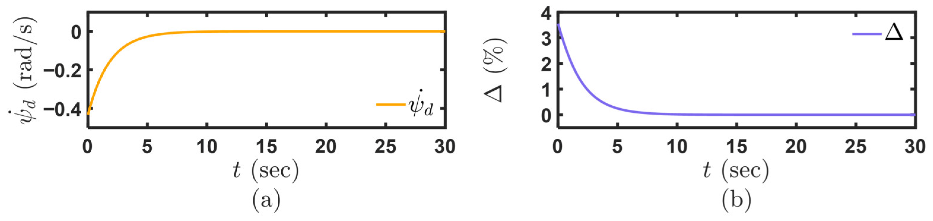
As shown in Figure 10, the maximum value of the linearization approximation error $\mathrm{\Delta }(t)$ at the initial moment is limited to within 4%, falling within the acceptable linearization threshold range, thereby verifying the feasibility of the linearization approximation. With the convergence of control input ${\dot{\psi }}_d(k)$, $\mathrm{\Delta }(t)$ asymptotically converges to zero. Moreover, under the state update mechanism, the model mismatch is compensated at each control cycle, thus leaving no residual linearization approximation error in the steady-state phase. The remaining simulation results are presented in Figure 11. It can be observed that even under extreme adverse initial conditions, the proposed control strategy still exhibits satisfactory control performance and steady-state accuracy, and the quadrotor MAV successfully achieves precise pose adjustment.

Figure 10. Simulation results: (a) Evolution of ${\dot{\psi }}_d(k)$. (b) Evolution of $\mathrm{\Delta }(t)$.

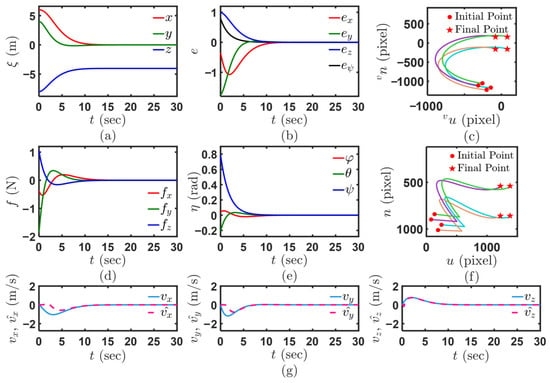
Figure 11. Simulation results: (a) MAV positions under ${\mathcal{F}}^w$. (b) Image feature error vectors. (c) Paths of target points in the virtual image plane. (d) Force vectors for the MAV. (e) MAV Euler angles. (f) Paths of target points in the real image plane. (g) MAV velocities and their observations.

6. Experiment Results

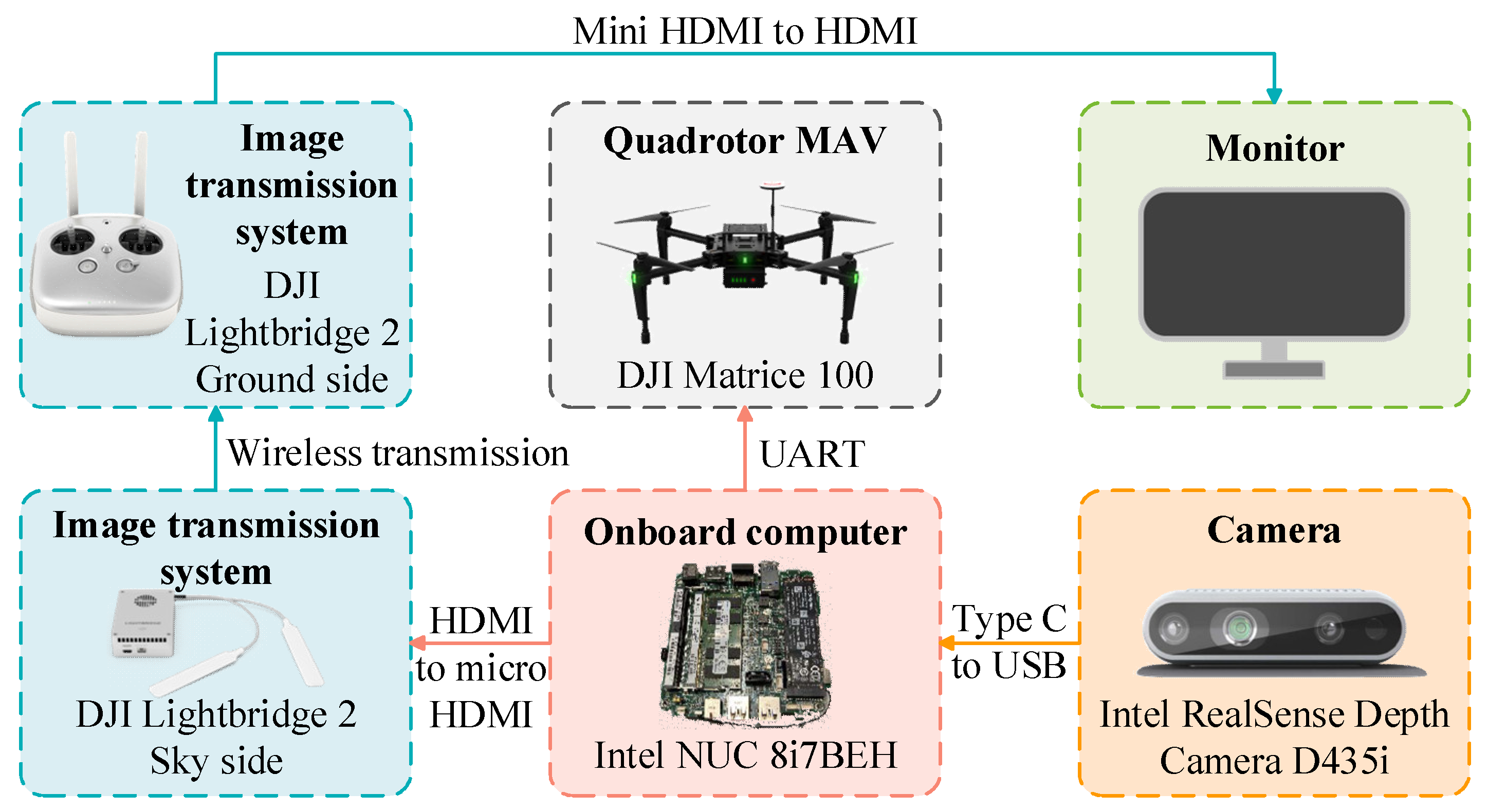
To further validate the proposed control strategy, a real-world experiment is conducted in this section using our previously developed experimental platform [25]. The hardware configuration comprises a quadrotor MAV equipped with dual cameras, an onboard computer, and an image transmission system. The MAV employed in this article is the DJI Matrice 100, manufactured by DJI in Shenzhen, China.

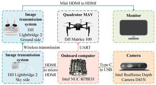
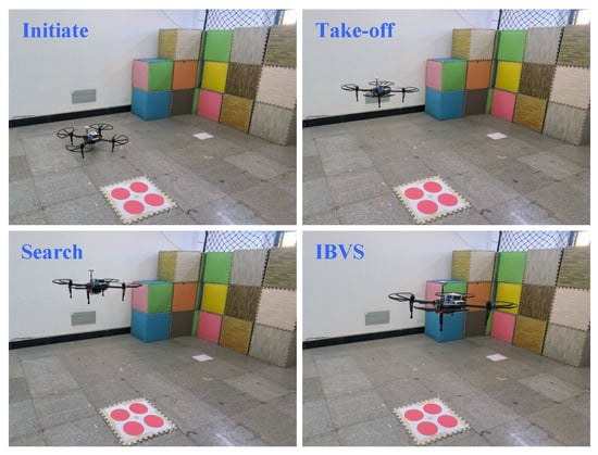
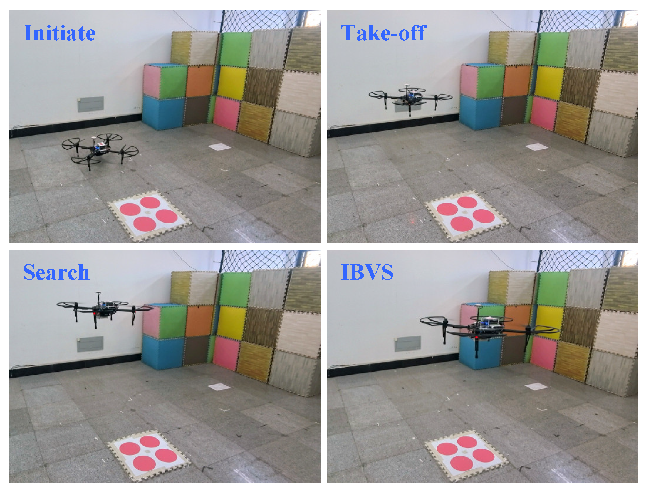
The onboard computer is installed with Ubuntu and the Robot Operating System (ROS) platform. The downward camera employed OpenCV algorithms to detect visual targets, thereby enabling the MAV to achieve IBVS. The MAV autonomously takes off and searches for the target, as detailed in our previous work [35]. During the take-off and search stages, the state information provided by VINS-Mono [43] is utilized to control the MAV flight via geometric tracking control [44]. Subsequently, in the IBVS stage, the MAV is controlled by the proposed control strategy. The experimental setup is illustrated in Figure 12.

Figure 12. Experimental setup of the MAV system.

Before the MAV takes off, the origin of ${\mathcal{F}}^w$ is set to coincide with the origin of ${\mathcal{F}}^b$ after initializing VINS-Mono. The target plane consists of four circular images. The coordinates of circle centers under ${\mathcal{F}}^w$ are set as ${[1.2,-0.2,0]}^T\mathrm{m}$, ${[1,-0.2,0]}^T\mathrm{m}$, ${[1,-0.4,0]}^T\mathrm{m}$, and ${[1.2,-0.4,0]}^T\mathrm{m}$. The MAV mass is $4.5 \mathrm{kg}$, and the camera focal length $\lambda$ is $1.8 \mathrm{mm}$. The desired vertical distance of the target relative to the camera is set as $z^{\ast }=1 \mathrm{m}$. The desired position and Euler angles of the MAV under ${\mathcal{F}}^w$ are set as ${[0,0,1]}^T\mathrm{m}$ and ${[0,0,0]}^T\mathrm{rad}$, respectively, with the parameter $a^{\ast }=9.1\times {10}^{-7}$.

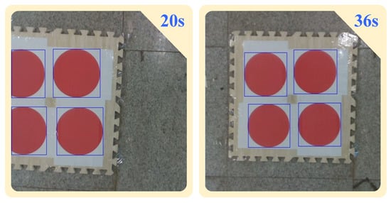
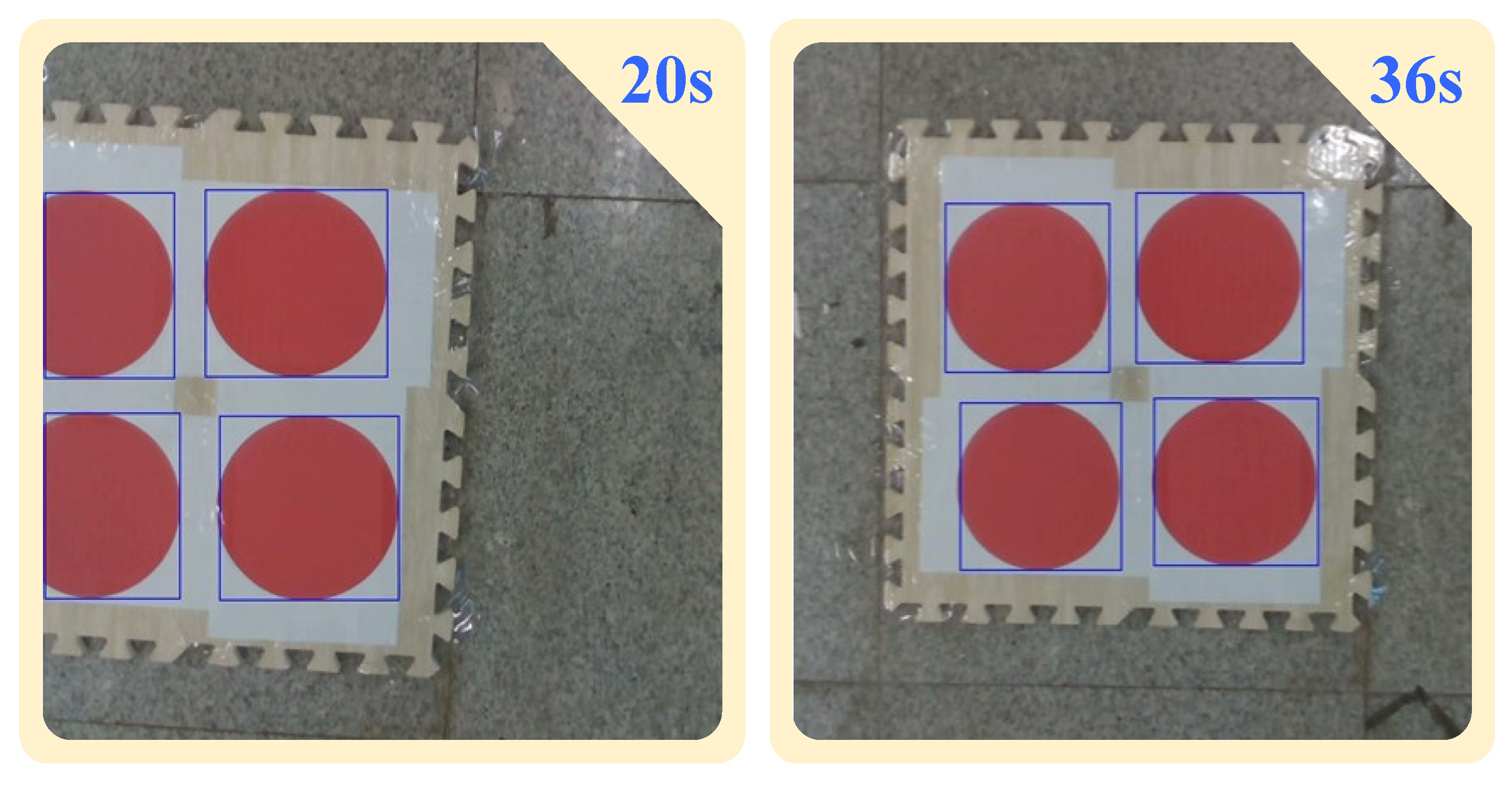
In the experiment, the closed-loop sampling frequency is $50 \mathrm{Hz}$ with a sampling time $dt$ of $0.02 \mathrm{s}$, which satisfies the real-time requirement. Observer gains are selected as ${\eta }_i=8$, ${\epsilon }_i=8$, and $\alpha =0.1$. ${}^1\rho _1$, ${}^2\rho _1$, ${}^3\rho _1$, ${}^1\rho _2$, ${}^2\rho _2$, and ${}^3\rho _2$ are set as $1\times {10}^4$, $1\times {10}^4$, $1.2\times {10}^4$, $1$, $1$, and $1.2$, respectively. Control weight matrices $Q$, $R$, and $Q_f$ are $\mathrm{blkdiag}(1500,1500,1500,5,8,8,8)$, $\mathrm{blkdiag}(0.5,0.5,0.5,0.5)$, and $\mathrm{blkdiag}(1300,1300,$$1300,3,8,8,8)$, respectively. Figure 13 provides several photos of the flight process. Images of the target plane captured by the downward camera are shown in Figure 14.

Figure 13. Experiment: Several photos of the flight process.

Figure 14. Experiment: The target plane captured on actual images during the IBVS stage.

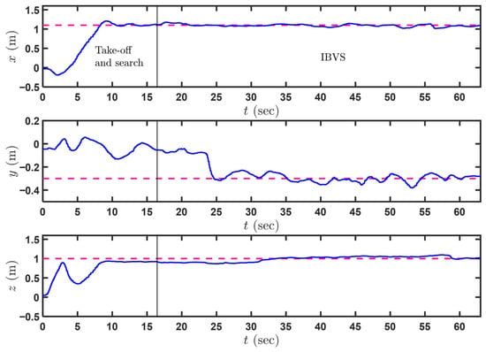
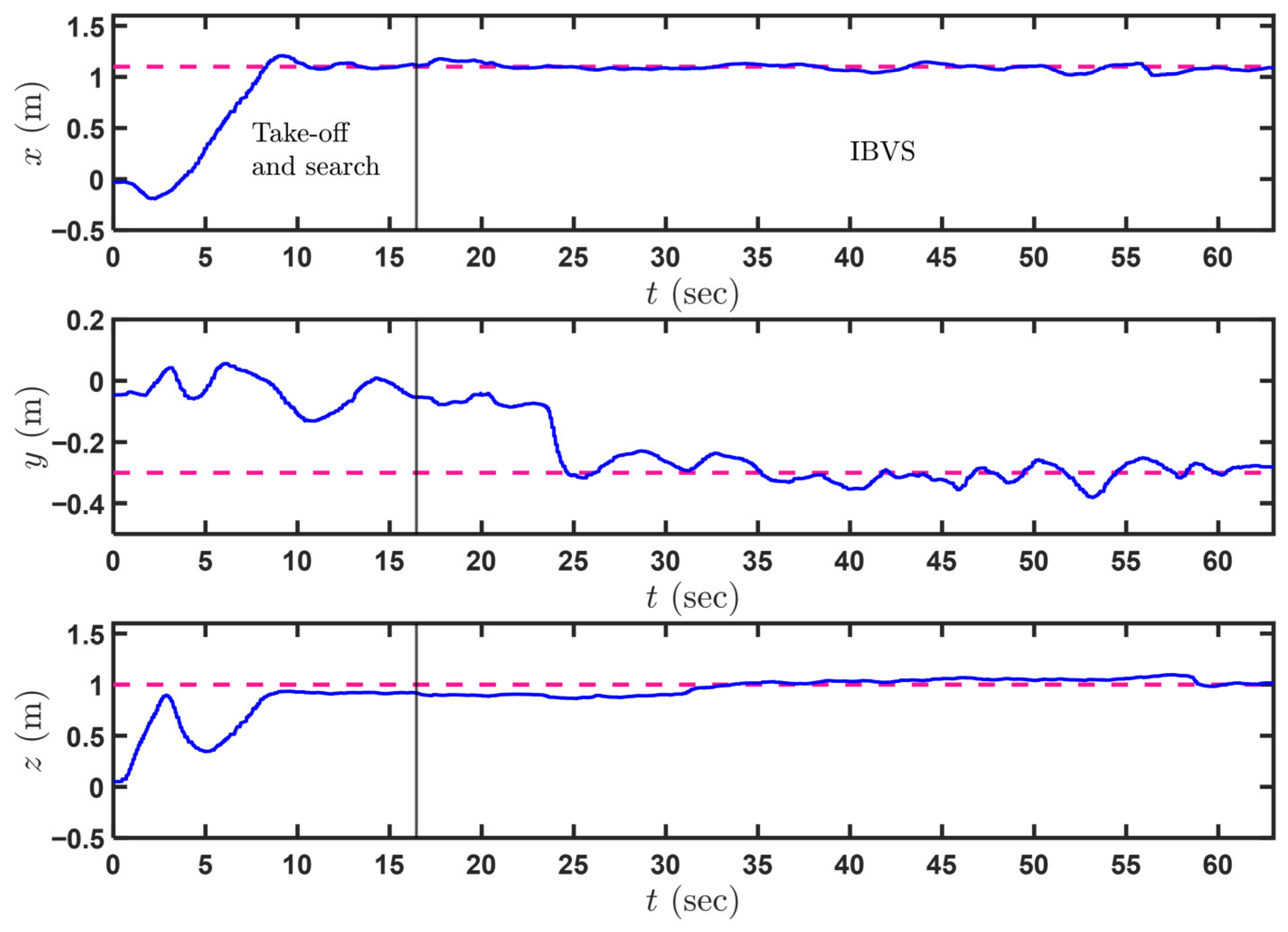
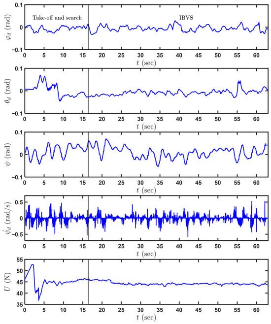
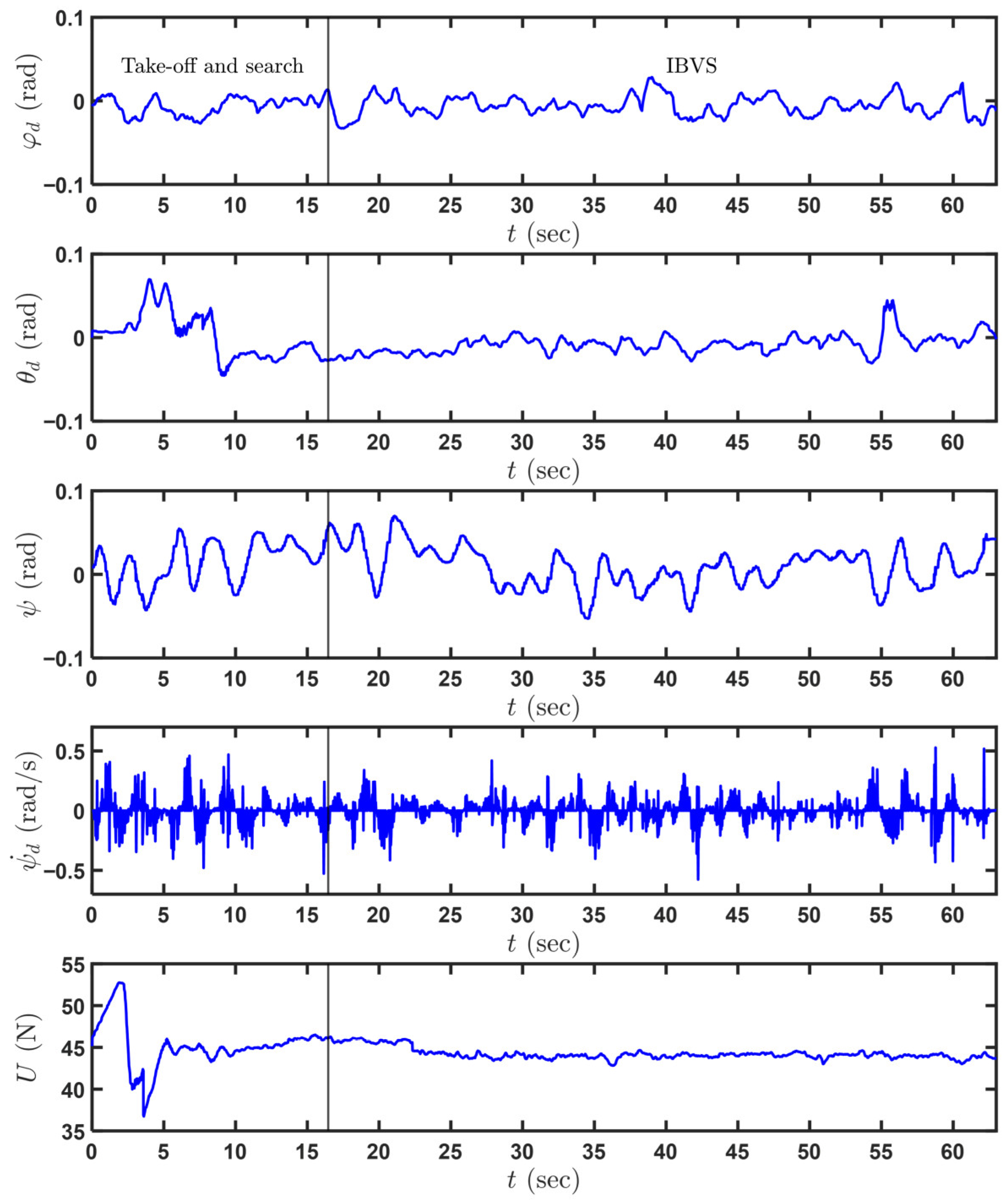
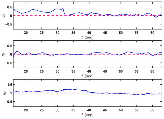
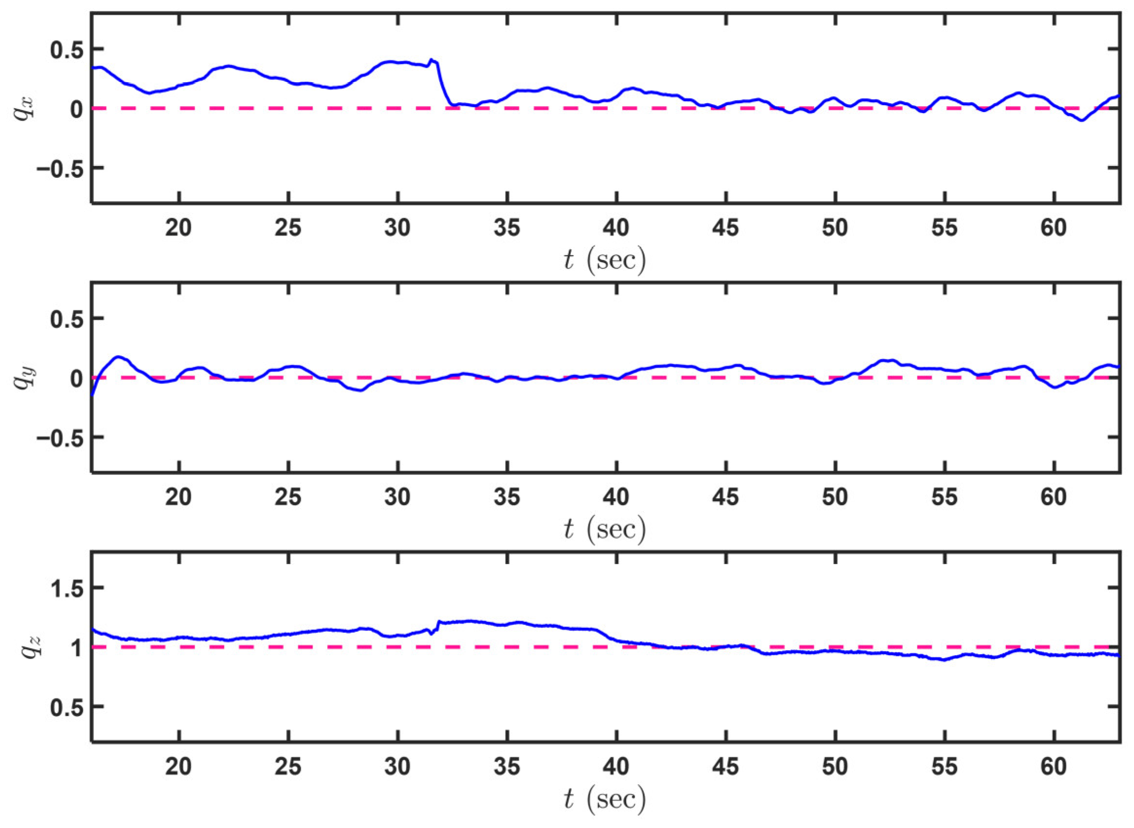
The experimental results are presented in Figure 15, Figure 16, Figure 17, Figure 18 and Figure 19. Figure 15 illustrates the positions of the MAV throughout the flight. Under the proposed control strategy, the MAV autonomously took off, searched for the target and stabilized at the desired position. From the evolution of the Euler angles and thrust control inputs provided in Figure 16, it can also be observed that the MAV continuously performs fine adjustments to its attitude above the target based on the image feature error. Figure 17 further illustrates the evolution of the image feature error.

Figure 15. Experiment results: Evolution of MAV positions during flight (solid lines: actual position; dashed lines: desired position during the IBVS stage).

Figure 16. Experiment results: Evolution of control inputs $U(k)$, ${\phi }_d(k)$, ${\theta }_d(k)$, ${\dot{\psi }}_d(k)$ and $\psi (k)$.

Figure 17. Experiment results: Evolution of image features (solid line: actual image features; dashed line: desired image features).

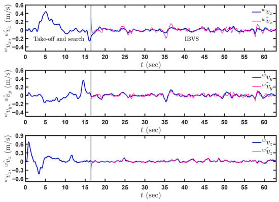
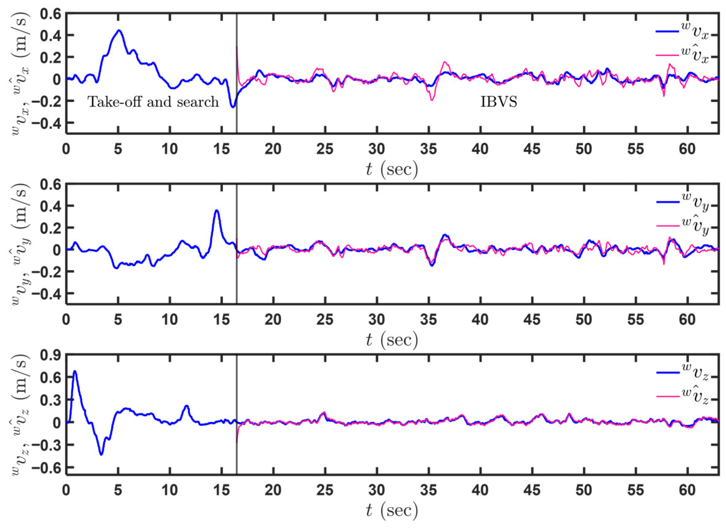
Figure 18. Experiment results: Evolution of MAV velocities and their observations.

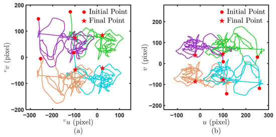
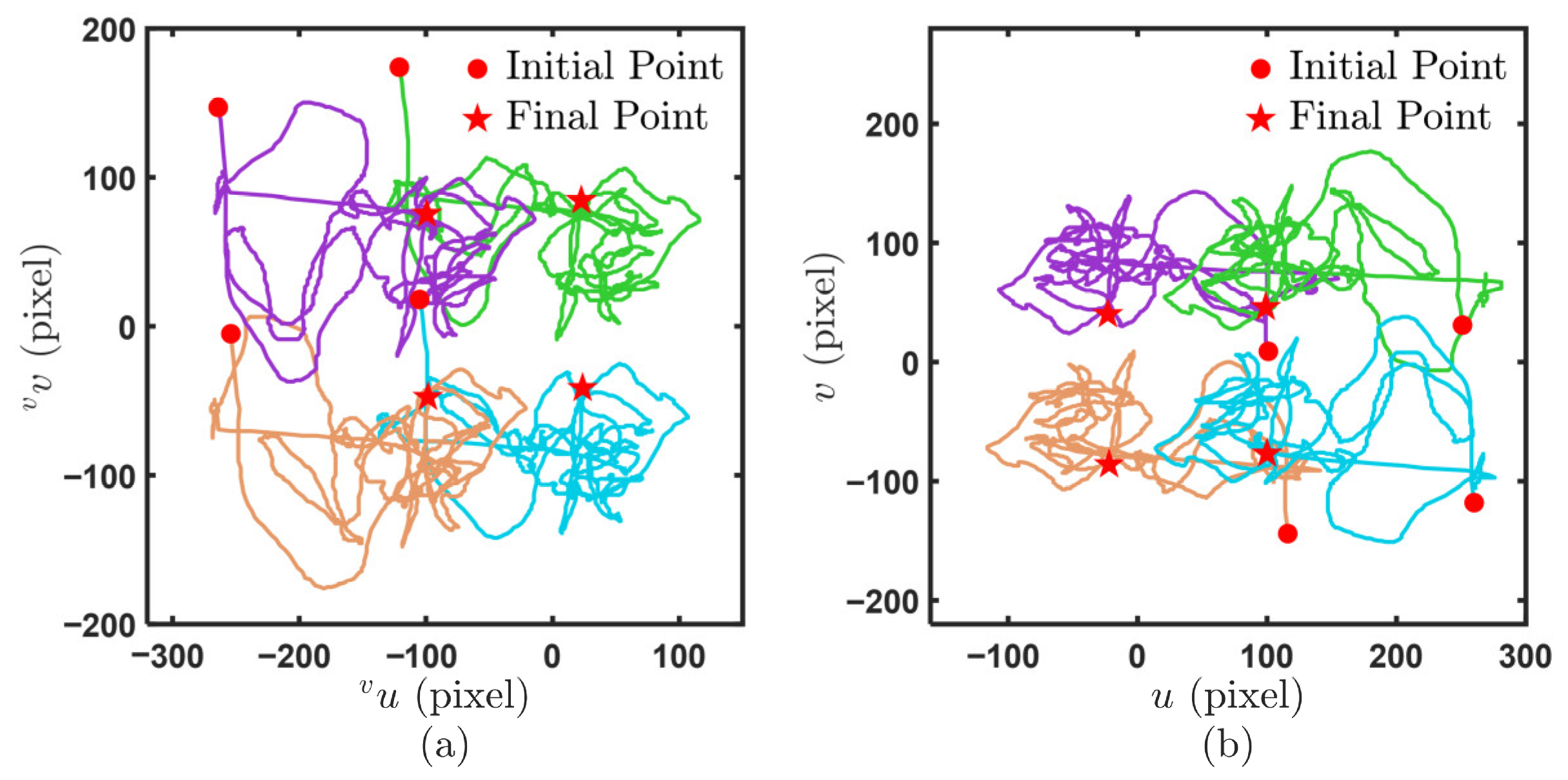
Figure 19. Experiment results: (a) Paths of target points in the virtual image plane. (b) Paths of target points in the virtual image plane.

Figure 18 presents the evolution of MAV velocities and their observed values. As shown, the proposed observer enables the observed velocities to converge rapidly to their actual values within a short time, demonstrating excellent observation performance. Figure 19 provides the trajectories of the centroid feature points of the circular images on the virtual and real image planes during the IBVS stage, respectively. The experimental results confirm that the proposed observation method can accurately estimate MAV linear velocity, and the proposed control strategy enables the MAV to hover stably at a specified position relative to the visual target.

7. Conclusions

This article presents an MPC method with velocity observation for the IBVS task of MAVs. By linear approximation, state updates, and rolling optimization, the method rapidly computes optimal control inputs to precisely adjust the MAV’s pose. During the take-off and search stages, the VINS-Mono algorithm provides real-time pose estimation, and target search is achieved through geometric tracking control. In the IBVS stage, image features for IBVS control are defined on the virtual image plane, and the linear velocity observer is developed. The image dynamics are approximated as linear via a first-order Taylor expansion, enabling the design of an MPC controller. By updating the system state with accurate and rapidly converging velocity estimates, steady-state errors are eliminated and control inputs are efficiently computed. The performance of the proposed observer and the control strategy is validated through simulations and experiments. The velocity observation method provides accurate MAV velocity estimation, and the MPC control strategy enables the MAV to achieve the desired trajectories in both image space and Cartesian space. The proposed control method is not applicable to strongly nonlinear systems with complex disturbance signals. Therefore, in future work, we will consider improving the control method to enhance the disturbance rejection capability of MAVs during IBVS tasks.

References

- Wu, J.; Sun, Y.; Li, D.; Shi, J.; Li, X.; Gao, L.; Yu, L.; Han, G.; Wu, J. An adaptive conversion speed Q-learning algorithm for search and rescue UAV path planning in unknown environments. IEEE Trans. Veh. Technol. 2023, 72, 15391–15404. [Google Scholar] [CrossRef] [Scilit]
- Yang, T.; Jiang, Z.; Sun, R.; Cheng, N.; Feng, H. Maritime search and rescue based on group mobile computing for unmanned aerial vehicles and unmanned surface vehicles. IEEE Trans. Ind. Inform. 2020, 16, 7700–7708. [Google Scholar] [CrossRef] [Scilit]
- Zhu, H.; Li, B.; Yin, H.; Zhang, X. Risk assessment based time-adjusted optimization for safe and fast flight of quadrotor UAVs. IEEE Trans. Veh. Technol. 2025, 74, 13658–13666. [Google Scholar] [CrossRef] [Scilit]
- Mebarki, R.; Lippiello, V.; Siciliano, B. Nonlinear visual control of unmanned aerial vehicles in GPS-denied environments. IEEE Trans. Robot. 2015, 31, 1004–1017. [Google Scholar] [CrossRef] [Scilit]
- Xu, W.; He, D.; Cai, Y.; Zhang, F. Robots’ state estimation and observability analysis based on statistical motion models. IEEE Trans. Control Syst. Technol. 2022, 30, 2030–2045. [Google Scholar] [CrossRef] [Scilit]
- Gao, C.; Wang, X.; Chen, X.; Chen, B. A hierarchical multi-UAV cooperative framework for infrastructure inspection and reconstruction. Control Theory Technol. 2024, 22, 394–405. [Google Scholar] [CrossRef] [Scilit]
- Shen, S.; Mulgaonkar, Y.; Michael, N.; Kumar, V. Vision-based state estimation for autonomous rotorcraft MAVs in complex environments. In Proceedings of the 2013 IEEE International Conference on Robotics and Automation (ICRA), Karlsruhe, Germany, 6–10 May 2013. [Google Scholar]
- Li, T.; Zhang, S.; Zhang, X.; Dong, Q.; Huang, J. SGS-Planner: A skeleton-guided spatiotemporal motion planner for flight in constrained space. IEEE/ASME Trans. Mechatron. 2025, 30, 191–202. [Google Scholar] [CrossRef] [Scilit]
- Singla, A.; Padakandla, S.; Bhatnagar, S. Memory-based deep reinforcement learning for obstacle avoidance in UAV with limited environment knowledge. IEEE Trans. Intell. Transp. Syst. 2021, 22, 107–118. [Google Scholar] [CrossRef]
- An, C.; Li, B.; Shi, W.; Zhang, X. Autonomous quadrotor UAV systems for dynamic platform landing with onboard sensors. Int. J. Robot. Autom. 2023, 38, 296–305. [Google Scholar] [CrossRef] [Scilit]
- Yang, K.; Bai, C.; She, Z.; Quan, Q. High-speed interception multicopter control by image-based visual servoing. IEEE Trans. Control Syst. Technol. 2025, 33, 119–135. [Google Scholar] [CrossRef] [Scilit]
- Wang, R.; Zhu, Z.; Zhang, X.; Fang, Y.; Li, B. Visual servoing trajectory tracking and depth identification for mobile robots with velocity saturation constraints. IEEE Trans. Ind. Electron. 2024, 71, 5950–5959. [Google Scholar] [CrossRef] [Scilit]
- Chen, Y.; Wu, Y.; Zhang, Z.; Miao, Z.; Zhong, H.; Zhang, H.; Wang, Y. Image-based visual servoing of unmanned aerial manipulators for tracking and grasping a moving target. IEEE Trans. Ind. Inform. 2023, 19, 8899. [Google Scholar] [CrossRef] [Scilit]
- Zhang, C.; Song, T.; Tao, H.; Jiang, T. Image-based fixed-time visual servoing control for UAV landing on a moving platform with visibility constraints. Nonlinear Dyn. 2025, 113, 29141–29156. [Google Scholar] [CrossRef] [Scilit]
- Xie, H.; Lynch, A.F.; Low, K.H.; Mao, S. Adaptive output-feedback image-based visual servoing for quadrotor unmanned aerial vehicles. IEEE Trans. Control Syst. Technol. 2020, 28, 1034–1041. [Google Scholar] [CrossRef] [Scilit]
- Wang, F.; Hu, S.; Zheng, J.; Zhou, K. Autonomous quadrotor with dynamic image-based visual servo for moving target tracking. In Proceedings of the 4th International Conference on Autonomous Unmanned Systems (ICAUS), Shenyang, China, 19–21 September 2024. [Google Scholar]
- Hamel, T.; Mahony, R. Visual servoing of an under-actuated dynamic rigid-body system: An image-based approach. IEEE Trans. Robot. Autom. 2002, 18, 187–198. [Google Scholar] [CrossRef] [Scilit]
- Zheng, D.; Wang, H.; Wang, J.; Chen, S.; Chen, W.; Liang, X. Image-based visual servoing of a quadrotor using virtual camera approach. IEEE/ASME Trans. Mechatron. 2017, 22, 972–982. [Google Scholar] [CrossRef] [Scilit]
- Guenard, N.; Hamel, T.; Mahony, R. A practical visual servo control for an unmanned aerial vehicle. IEEE Trans. Robot. 2008, 24, 331–340. [Google Scholar] [CrossRef] [Scilit]
- Chaumette, F. Image moments: A general and useful set of features for visual servoing. IEEE Trans. Robot. 2004, 20, 713–723. [Google Scholar] [CrossRef] [Scilit]
- Jabbari, H.; Oriolo, G.; Bolandi, H. Dynamic IBVS control of an underactuated UAV. In Proceedings of the 2012 IEEE International Conference on Robotics and Biomimetics (ROBIO), Guangzhou, China, 11–14 December 2012. [Google Scholar]
- Bourquardez, O.; Mahony, R.; Guenard, N.; Chaumette, F.; Hamel, T.; Eck, L. Image-based visual servo control of the translation kinematics of a quadrotor aerial vehicle. IEEE Trans. Robot. 2009, 25, 743–749. [Google Scholar] [CrossRef] [Scilit]
- Yi, X.; Luo, B.; Zhao, Y. Adaptive dynamic programming-based visual servoing control for quadrotor. Neurocomputing 2022, 504, 251–261. [Google Scholar] [CrossRef] [Scilit]
- Shi, L.; Li, B.; Shi, W. Vision-based UAV adaptive tracking control for moving targets with velocity observation. Trans. Inst. Meas. Control. 2024, 46, 2255–2265. [Google Scholar] [CrossRef] [Scilit]
- Chen, Y.; Li, B.; Shi, W.; Zhang, X. Image-based visual servoing of micro aerial vehicles with robust observation and output feedback. IEEE Trans. Control Syst. Technol. 2025, 33, 1995–2004. [Google Scholar] [CrossRef] [Scilit]
- Ozawa, R.; Chaumette, F. Dynamic visual servoing with image moments for a quadrotor using a virtual spring approach. In Proceedings of the 2011 IEEE International Conference on Robotics and Automation (ICRA), Shanghai, China, 9–13 May 2011. [Google Scholar]
- Yan, H.; Yang, K.; Cheng, Y.; Wang, Z.; Li, D. Precise interception flight targets by image-based visual servoing of multicopter. IEEE. Trans. Ind. Electron. 2025, 72, 11499–11509. [Google Scholar] [CrossRef] [Scilit]
- Jabbari, H.; Bolandi, H. Robust vision-based control of an underactuated flying robot tracking a moving target. Trans. Inst. Meas. Control. 2014, 36, 411–424. [Google Scholar]
- Fink, G.; Xie, H.; Lynch, A.F.; Jagersand, M. Experimental validation of dynamic visual servoing for a quadrotor using a virtual camera. In Proceedings of the 2015 International Conference on Unmanned Aircraft Systems (ICUAS), Denver, CO, USA, 9–12 June 2015. [Google Scholar]
- He, W.; Yuan, L. Image-based finite-time visual servoing of a quadrotor for tracking a moving target. Nonlinear Dyn. 2023, 111, 5307–5328. [Google Scholar] [CrossRef] [Scilit]
- Zhang, X.; Fang, Y.; Zhang, X.; Jiang, J.; Chen, X. Dynamic image-based output feedback control for visual servoing of multirotors. IEEE Trans. Ind. Inform. 2020, 16, 7624–7636. [Google Scholar] [CrossRef] [Scilit]
- Zhang, H.; Wang, R.; Zhang, X.; Li, T.; Zhang, S.; Zhang, X. CBF based geometric visual servoing control for quadrotors with FOV constraint. In Proceedings of the 2022 International Conference on Autonomous Unmanned Systems (ICAUS), Xi’an, China, 23–25 September 2022. [Google Scholar]
- Lin, J.; Wang, Y.; Miao, Z.; Fan, S.; Wang, H. Robust observer-based visual servo control for quadrotors tracking unknown moving targets. IEEE/ASME Trans. Mechatron. 2023, 28, 1268–1279. [Google Scholar] [CrossRef] [Scilit]
- Yi, X.; Luo, B.; Zhao, Y. Neural network-based robust guaranteed cost control for image-based visual servoing of quadrotor. IEEE Trans. Neural Netw. Learn. Syst. 2024, 35, 12693–12705. [Google Scholar] [CrossRef] [Scilit]
- Shi, L.; Li, B.; Shi, W.; Zhang, X. Visual servoing of quadrotor UAVs for slant targets with autonomous object search. Proc. Inst. Mech. Eng. Part I J. Syst. Control Eng. 2023, 237, 791–804. [Google Scholar] [CrossRef] [Scilit]
- Lin, J.; Wang, Y.; Miao, Z.; Wang, H.; Fierro, R. Robust image-based landing control of a quadrotor on an unpredictable moving vehicle using circle features. IEEE Trans. Autom. Sci. Eng. 2023, 20, 1429–1440. [Google Scholar] [CrossRef] [Scilit]
- Rawlings, J.B.; Mayne, D.Q.; Diehl, M.M. Model Predictive Control: Theory, Computation, and Design, 2nd ed.; Nob Hill Publishing: Madison, WI, USA, 2017; pp. 1–435. [Google Scholar]
- Roque, P.; Bin, E.; Miraldo, P.; Dimarogonas, D.V. Fast model predictive image-based visual servoing for quadrotors. In Proceedings of the 2020 IEEE/RSJ International Conference on Intelligent Robots and Systems (IROS), Las Vegas, NV, USA, 24 October 2020–24 January 2021. [Google Scholar]
- Zhang, K.; Shi, Y.; Sheng, H. Robust nonlinear model predictive control based visual servoing of quadrotor UAVs. IEEE/ASME Trans. Mechatron. 2021, 26, 700–708. [Google Scholar] [CrossRef] [Scilit]
- Nicosia, S.; Tomei, P.; Tornambè, A. An approximate observer for a class of nonlinear systems. Syst. Control Lett. 1989, 13, 43–51. [Google Scholar] [CrossRef] [Scilit]
- Khalil, H. Nonlinear Systems, 3rd ed.; Prentice Hall: Upper Saddle River, NJ, USA, 2002; pp. 551–625. [Google Scholar]
- Tornambè, A. High-gain observers for non-linear systems. Int. J. Syst. Sci. 1992, 23, 1475–1489. [Google Scholar] [CrossRef] [Scilit]
- Qin, T.; Li, P.; Shen, S. VINS-Mono: A robust and versatile monocular visual-inertial state estimator. IEEE Trans. Robot. 2018, 34, 1004–1020. [Google Scholar] [CrossRef] [Scilit]
- Lee, T.; Leok, M.; McClamroch, N.H. Geometric tracking control of a quadrotor UAV on SE(3). In Proceedings of the 49th IEEE Conference on Decision and Control (CDC), Atlanta, GA, USA, 15–17 December 2010. [Google Scholar]
Disclaimer/Publisher’s Note: The statements, opinions and data contained in all publications are solely those of the individual author(s) and contributor(s) and not of MDPI and/or the editor(s). MDPI and/or the editor(s) disclaim responsibility for any injury to people or property resulting from any ideas, methods, instructions or products referred to in the content. |
© 2026 by the authors. Licensee MDPI, Basel, Switzerland. This article is an open access article distributed under the terms and conditions of the Creative Commons Attribution (CC BY) license.