Fuzzy Granular Ball-Based Attribute Reduction for Interval-Valued Decision Systems

Abstract

Feature selection is a core step in data analysis and is referred to as attribute reduction in rough set theory. Granular ball computing has emerged as a novel data analysis paradigm characterized by high computational efficiency, robustness, and scalability. However, in previous attribute reduction methods for interval numbers, the construction of tolerance classes and the reduction iteration process suffer from inefficiency. To address these limitations, this paper proposes an efficient attribute reduction method based on fuzzy interval-valued granular balls. This method integrates fuzzy interval-valued granular balls with an acceleration strategy based on the positive region. Specifically, we first construct tolerance classes efficiently using fuzzy interval-valued granular balls, thereby enabling a reasonable partition of the universe. We then remove redundant objects in the positive region during the reduction iteration to avoid unnecessary computations. On this basis, we further propose a conditional entropy-based algorithm for attribute reduction. Experimental results show that this algorithm substantially improves computational efficiency while maintaining high classification accuracy.

1. Introduction

Proposed by Pawlak [1], rough set theory (RST) provides an effective method for analyzing uncertainty in complex datasets and has been applied in various areas. Attribute reduction [2,3] is a core research topic in RST. In practical applications, attribute reduction can effectively reduce data dimensionality, decrease computational complexity, and improve the robustness of learning models. With the increasing complexity of modern datasets, various reduction methods have been continuously developed. Miao et al. [4] investigated discernibility matrices corresponding to different reduction objectives. They defined generalized decision reduction and indiscernibility-relation-based reduction in decision systems. In incompletely labeled data systems, Dai et al. [5] proposed a label distribution-based reduction method. Yang et al. [6] designed an effective reduction method in fuzzy rough sets. Yuan et al. [7] introduced a soft label learning mechanism and designed a novel feature selection method under weakly supervised scenarios.

Nevertheless, data often exhibit the characteristics of interval numbers in practical scenarios. Consequently, equivalence relation-based attribute reduction cannot be applied to an interval-valued decision system (INDS). To tackle this problem, researchers have extensively investigated attribute reduction algorithms in an INDS [8,9]. For instance, based on the rough approximations, Gong et al. [10] constructed a knowledge discovery framework. Based on mutual information and attribute dependency, Xu et al. [11] designed heuristic reduction algorithms. They also provided a global feature reduction suitable for a large-scale INDS. Based on multiple measures, Dai et al. [12] designed a reduction method from an information-theoretic perspective. Xie et al. [13] introduced rough entropy and constructed the information structure of an INDS. Based on attribute weights, Zhang et al. [14] proposed an algorithm to remove redundant attributes. Liu et al. [15] formulated a fuzzy similarity relationship and developed a reduction algorithm. Dai et al. [16] proposed a novel reduction method based on fuzzy discernibility pairs. Xu et al. [17,18] investigated reduction methods for a multi-source INDS by combining optimization strategies with information fusion. Based on graph theory, Zhang et al. [19] designed an algorithm to remove redundant attributes.

As a novel method for handling complex data, the granular ball effectively utilizes label information and sample distribution characteristics. Xia et al. [20] constructed a classification framework based on granular computing and used it to classify data. In recent years, a large number of granular ball-based attribute reduction algorithms [21,22,23] were studied. To address the inefficiency of traditional radius computation, Xia et al. [24] designed a novel rough set model that adaptively generates the neighborhood radius and then developed a feature selection algorithm. Chen et al. [25] designed a reduction method that adaptively generated reducts by sorting granular balls. By adopting a division-oriented method, Xia et al. [26] accelerated granular ball generation during the attribute reduction process. To handle data with label noise, Peng et al. [27] constructed a model with variable parameters and proposed a reduction algorithm. By merging fuzziness with granular balls, Ji et al. [28] introduced a new definition for granular balls and proposed a novel reduction method. Xia et al. [29] integrated granular balls into rough set theory and represented two rough sets using a unified granular ball model. Chen et al. [30] introduced the granular ball into the variable precision rough set model and proposed a novel feature selection algorithm. In addition, granular ball-based methods have been extended to label distribution learning and labeling confidence-based feature selection [31,32], as well as outlier detection [33]. Gao et al. [34] proposed a novel granular ball model based on three-way decision theory and applied it to outlier detection. Wang et al. [35] proposed a novel outlier detection method that significantly enhances detection efficiency while ensuring detection accuracy.

To better position the proposed method with respect to existing studies, Table 1 summarizes representative related works from the perspectives of problem setting and efficiency strategy.

Table 1. Comparison of representative related works and the proposed method.

Method	Problem Setting	Efficiency Strategy
ARIE [11]	Reduction in INDS	Heuristic attribute selection
ARCE [12]	Reduction in INDS	Conditional entropy evaluation
ARRE [13]	Reduction in INDS	Rough entropy evaluation
GBNRS [24]	Reduction in classical decision systems	Granular ball acceleration
FGBERS [28]	Reduction in fuzzy rough set	Fuzzy granular ball acceleration
FRFIGB	Reduction in INDS	Granular ball acceleration and positive-region acceleration

• Motivation

As shown in Table 1, existing reduction methods for INDS are mainly based on traditional tolerance relations to construct tolerance classes, which usually lead to high computational cost in both tolerance class construction and the reduction process. In contrast, a granular ball can improve efficiency, but existing methods cannot be applied to INDS.

• Novelties

To address this issue, the main contributions of this paper are summarized as follows:

(1)

This paper proposes a fuzzy interval-valued granular ball (FIGB). FIGB provides a fast and reasonable partition of the universe, thereby enabling the rapid and adaptive construction of tolerance classes for each object.

(2)

Based on the rank preservation of attribute significance, an acceleration strategy is proposed to improve the efficiency of the reduction process.

(3)

This paper proposes an efficient attribute reduction algorithm. The algorithm integrates FIGB with an acceleration strategy. During the reduction process, we remove redundant positive-region objects to avoid unnecessary computations in each iteration, thereby further improving efficiency.

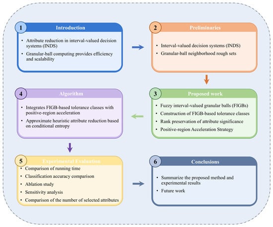
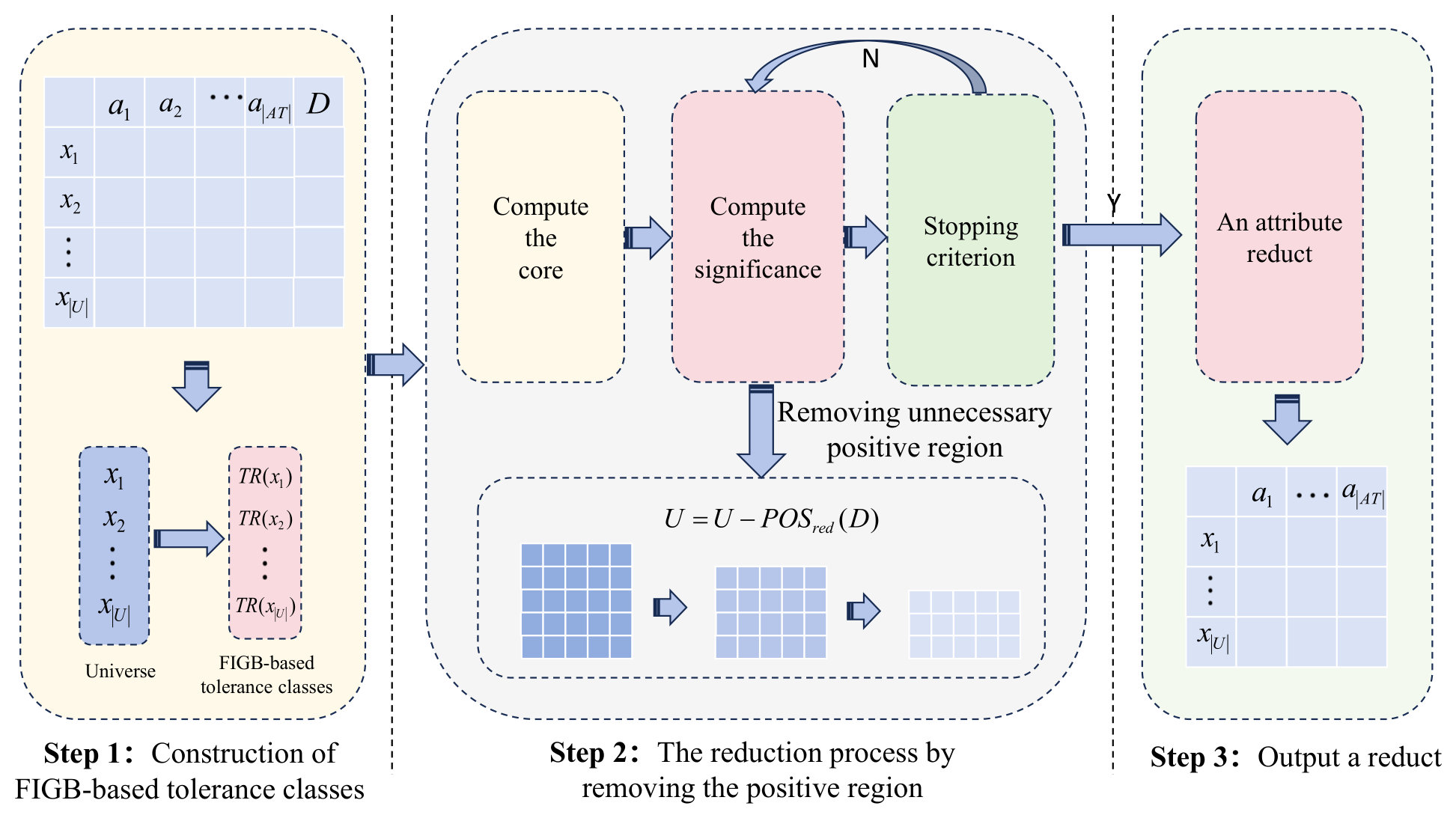
The rest of this paper is structured as follows: Section 2 introduces the basic concepts of INDS and granular ball neighborhood rough sets. Section 3 proposes the construction of FIGB and an acceleration strategy based on the positive region. Section 4 provides a detailed description of the proposed algorithms. Section 5 presents experimental results and corresponding discussions. Section 6 concludes the paper. Figure 1 illustrates the framework of this paper.

Figure 1. Framework.

2. Preliminaries

In this section, we briefly review the basic concepts of an interval-valued decision system and granular ball neighborhood rough sets.

2.1. An Interval-Valued Decision System

In rough set theory, interval numbers are represented by a quadruple as follows:

Definition 1

([36]). Let $INIS=(\mathcal{U},\mathcal{A},\mathcal{V},\mathcal{F})$ be an interval-valued information system, where $\mathcal{U}=\{x_1,x_2,\dots ,x_{\left|\mathcal{U}\right|}\}$ is the universe, $\mathcal{A}=\{a_1,a_2,\dots ,a_{\left|A\right|}\}$ is the set of attributes, $\mathcal{V}={\bigcup }_{a_k\in \mathcal{A}}{\mathcal{V}}_{a_k}$, ${\mathcal{V}}_{a_k}$ is the domain of attribute $a_k$, the information function is given by $\mathcal{F}:\mathcal{U}\times \mathcal{A}\to {\mathcal{V}}_{\mathcal{A}}$. If $\mathcal{A}=\mathcal{AT}\cup \mathcal{D}$, $\mathcal{AT}\cap \mathcal{D}=⌀$, and $\mathcal{D}\ne ⌀$, then $(\mathcal{U},\mathcal{AT}\cup \mathcal{D},\mathcal{V},\mathcal{F})$ is defined as an $INDS$, where $\mathcal{AT}$ is the conditional attribute set, and $\mathcal{D}$ is the decision attribute set.

In an $INDS$, the operations on interval numbers are defined as follows, including the intersection and union of two interval numbers.

Definition 2

([37]). In an $INDS$, $\forall x_h,x_l\in \mathcal{U}$, $a_k\in \mathcal{AT}$, $x_h^k=[m_h^k,n_h^k]$ and $x_l^k=[m_l^k,n_l^k]$, the intersection and union of $x_h^k$ and $x_l^k$ are defined as follows

$$x_h^k\cap x_l^k=\left\{\begin{array}{cc}[\max (m_h^k,m_l^k),\min (n_h^k,n_l^k)],\hfill & \max (m_h^k,m_l^k)\le \min (n_h^k,n_l^k),\hfill \\ ⌀,\hfill & \mathit{otherwise}.\hfill \end{array}\right.$$

(1)

$$x_h^k\cup x_l^k=\left\{\begin{array}{cc}[\min (m_h^k,m_l^k),\max (n_h^k,n_l^k)],\hfill & \max (m_h^k,m_l^k)\le \min (n_h^k,n_l^k),\hfill \\ m_h^k,n_h^k]\cup [m_l^k,n_l^k],\hfill & \mathit{otherwise}.\hfill \end{array}\right.$$

(2)

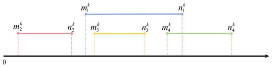
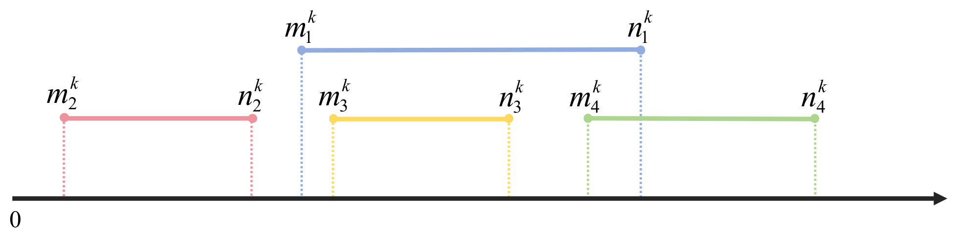
Figure 2 presents three basic relationships between interval numbers: disjointness, inclusion, and intersection. These relationships are the basis for the subsequent interval operations and similarity definition.

Figure 2. The relationships of interval numbers.

(1)

$[m_1^k,n_1^k]$ and $[m_2^k,n_2^k]$ are disjoint;

(2)

$[m_1^k,n_1^k]$ contains $[m_3^k,n_3^k]$;

(3)

$[m_1^k,n_1^k]$ and $[m_4^k,n_4^k]$ intersect.

Based on the above operations, the similarity degree between two interval numbers is defined as follows:

Definition 3

([38]). In an $INDS$, $\forall a_k\in \mathcal{AT}$, the Jaccard similarity degree between $x_h^k$ and $x_l^k$ is defined as

$$C_{hl}^k={\displaystyle \frac{|x_h^k\cap x_l^k|}{|x_h^k\cup x_l^k|}},$$

(3)

Definition 4

([12]). In an $INDS$, $\mathcal{P}\subseteq \mathcal{AT}$, a similarity degree threshold $\gamma \in [0,1]$, the γ-tolerance relation is defined as

$${\mathbb{T}}_{\mathcal{P}}^{\gamma }=\left\{(x_h,x_l)\in \mathcal{U}\times \mathcal{U}|C_{hl}^k\ge \gamma ,\forall a_k\in \mathcal{P}\right\}.$$

(4)

Based on the $\gamma$-tolerance relation of interval numbers, the tolerance class is defined as follows:

Definition 5

([12]). In an $INDS$, $\mathcal{P}\subseteq \mathcal{AT}$, $\gamma \in [0,1]$, the γ-tolerance class of object $x_h$ is defined as

$${\mathbb{S}}_{\mathcal{P}}^{\gamma }\left(x_h\right)=\left\{x_h\in \mathcal{U}|(x_l,x_h)\in {\mathbb{T}}_{\mathcal{P}}^{\gamma }\right\}.$$

(5)

If two objects satisfy the $\gamma$-tolerance relation, then they belong to each other’s tolerance class. Based on the $\gamma$-tolerance class, the lower and upper approximations in an $INDS$ are given as follows:

Definition 6

([12]). In an $INDS$, $\mathcal{P}\subseteq \mathcal{AT}$, $X\subseteq \mathcal{U}$, $\gamma \in [0,1]$, the lower approximation $\left(LA\right)$ and upper approximation $\left(UA\right)$ of X are defined as

$$\underline{ap{r}_P^{\gamma }}\left(X\right)=\left\{x_h\in \mathcal{U}|{\mathbb{S}}_{\mathcal{P}}^{\gamma }\left(x_h\right)\subseteq X\right\},$$

(6)

$$\overline{ap{r}_P^{\gamma }}\left(X\right)=\left\{x_h\in \mathcal{U}|{\mathbb{S}}_{\mathcal{P}}^{\gamma }\left(x_h\right)\cap X\ne ⌀\right\}.$$

(7)

2.2. Granular Ball Neighborhood Rough Sets

The fundamental concepts of granular ball neighborhood rough sets are reviewed in this subsection.

Definition 7

([29]). Let $DS=(\mathcal{U},\mathcal{AT}\cup \mathcal{D},\mathcal{V},\mathcal{F})$ be a decision system. A granular ball $G{B}_{\tau }=\{x_h\mid h=1,2,\dots ,\omega \}$, where $x_h$ is a single value. The center c and radius r of $G{B}_{\tau }$ are defined as

$$c={\displaystyle \frac{1}{\omega }}{\displaystyle \sum _{h=1}^{\omega }}{x}_h,$$

(8)

$$r=\underset{h=1,2,\dots ,\omega }{\max }d(x_h,c),$$

(9)

where $d(x_h,c)$ denotes the Euclidean distance between $x_h$ and c, r is the maximum distance between the center and other objects.

Based on the above definition, the neighborhood can be adaptively generated for each object. The neighborhood of an object is defined as follows:

Definition 8

([24]). $G{B}_{\tau }$ is the τ-th granular ball. $\forall x_h\in G{B}_{\tau }$, the neighborhood of $x_h$ is defined as

$$\sigma \left(x_h\right)=\{x_l\in G{B}_{\tau }\mid d(x_l,c_{\tau })\le r_{\tau }\},$$

(10)

For any object within a granular ball, other objects whose distance to the center of the ball is less than the radius are considered to belong to the neighborhood of that object.

Definition 9

([24]). In a $DS$, $\mathcal{P}\subseteq \mathcal{AT}$, $X\subseteq \mathcal{U}$. The lower approximation $\left(LA\right)$ and upper approximation $\left(UA\right)$ of X are defined as

$$\underline{\mathcal{P}}X=\{x_h\in \mathcal{U}\mid x_h\in G{B}_{\tau }\left(\mathcal{P}\right),\sigma \left(x_h\right)\subseteq X\},$$

(11)

$$\overline{\mathcal{P}}X=\{x_h\in \mathcal{U}\mid x_h\in G{B}_{\tau }\left(\mathcal{P}\right),\sigma \left(x_h\right)\cap X\ne ⌀\},$$

(12)

where $G{B}_{\tau }\left(\mathcal{P}\right)$ denotes the τ-th granular ball.

3. Construction of Tolerance Classes Based on FIGB and Rank Preservation of Attribute Significance

In this section, Section 3.1 proposes fuzzy interval-valued granular balls and rapidly constructs tolerance classes based on them. On this basis, Section 3.2 proposes the rank preservation property of the attribute significance measure to improve the efficiency of attribute reduction.

3.1. Construction of FIGB-Based Tolerance Classes

Considering the high efficiency of granular balls in partitioning the universe, we propose fuzzy interval-valued granular balls to construct tolerance classes and achieve an efficient partition of the universe. In the process of generating fuzzy interval-valued granular balls, we adopt the fuzzy c-means clustering method for symbolic interval numbers (IFCM) [39]. IFCM aims to partition objects into multiple clusters by maximizing intra-cluster similarity. The basic definitions of IFCM are summarized as follows:

Definition 10

([39]). In an $INDS$, $\forall a_k\in \mathcal{AT}$, $Q=\{Q_1,\dots ,Q_z\}$ is a partition of $\mathcal{U}$, $q_i^k=[{\alpha }_i^k,{\beta }_i^k]$ is the i-th cluster center. $x_h\in \mathcal{U}$, the distance between $x_h^k$ and $q_i^k$ is defined as

$$d(x_h^k,q_i^k)={({(m_h^k-{\alpha }_i^k)}^2+{(n_h^k-{\beta }_i^k)}^2)}^{1/2}.$$

(13)

In the process of clustering, we assign objects to clusters based on their membership degrees. The membership degree between an object and a cluster center is defined as follows:

Definition 11

([39]). In an $INDS$, $\forall x_h\in \mathcal{U}$, $a_k\in \mathcal{AT}$, the membership degree between $x_h^k$ and $q_i^k$ is as follows

$$u_{ih}={\left[{\displaystyle \sum _{p=1}^z}{\left({\displaystyle \frac{{(m_h^k-{\alpha }_i^k)}^2+{(n_h^k-{\beta }_i^k)}^2}{{(m_h^k-{\alpha }_p^k)}^2+{(n_h^k-{\beta }_p^k)}^2}}\right)}^{{\displaystyle \frac{1}{m-1}}}\right]}^{-1},$$

(14)

where $u_{ih}\ge 0$ and ${\sum }_{i=1}^z{u}_{ih}=1$, for $i=1,2,\dots ,z$. Here, $m=2$ by default, z denotes the number of clusters.

Each object is assigned to the cluster with the highest membership degree in the process of clustering. Based on membership degrees, the formula for updating the cluster centers is defined as follows:

Definition 12

([39]). In an $INDS$, $\forall a_k\in \mathcal{AT}$, $x_h\in \mathcal{U}$, the cluster center $q_i^k$ is updated as follows

$${\alpha }_i^k={\displaystyle \frac{{\sum }_{h=1}^{\left|\mathcal{U}\right|}{\left(u_{ih}\right)}^2{m}_h^k}{{\sum }_{h=1}^{\left|\mathcal{U}\right|}{\left(u_{ih}\right)}^2}},{\beta }_i^k={\displaystyle \frac{{\sum }_{h=1}^{\left|\mathcal{U}\right|}{\left(u_{ih}\right)}^2{n}_h^k}{{\sum }_{h=1}^{\left|\mathcal{U}\right|}{\left(u_{ih}\right)}^2}},$$

(15)

Due to the efficiency, robustness, and scalability of granular balls in classification and reduction, we propose a fuzzy interval-valued granular ball (FIGB).

Definition 13.

In an $INDS$, a fuzzy interval-valued granular ball is denoted by $FIGB=\{x_h\mid h=1,2,\dots ,|FIGB\left|\right\}$, $\forall a_k\in \mathcal{AT}$, the center c and radius r of $FIGB$ are defined as

$$c=\left[{\displaystyle \frac{1}{\left|FIGB\right|}}\sum _{x_h\in FIGB}{m}_h^k,{\displaystyle \frac{1}{\left|FIGB\right|}}\sum _{x_h\in FIGB}{n}_h^k\right],$$

(16)

$$r=d(x_u,c),$$

(17)

where $x_h=[m_h^k,n_h^k]$, $x_u$ has the minimum membership degree with the center c.

Definition 13 defines the fuzzy interval-valued granular ball. It gives the center and radius of the fuzzy interval-valued granular ball and is used to represent similar interval-valued objects. A fuzzy interval-valued granular ball is defined as the set of objects whose distance to the center is less than the radius.

Definition 14.

Given a $FIGB$, which is composed of k classes of objects, such that ${\bigcup }_{i=1}^k{l}_i=FIGB$ and ${\bigcap }_{i=1}^k{l}_i=⌀$. The purity of $FIGB$ is defined as

$$T\left(FIGB\right)={\displaystyle \frac{{\max }_{i=1,2,\dots ,k}\left|l_i\right|}{\left|FIGB\right|}},$$

(18)

where $l_i$ represents the i-th label class in $FIGB$.

The purity of the fuzzy interval-valued granular ball is used to measure the decision consistency inside the granular ball. $T\left(FIGB\right)$ measures the proportion of the objects with the majority label in $FIGB$. During the generation of $FIGB$s, the purity of each $FIGB$ is used as the splitting criterion. If the purity does not satisfy a given threshold, the $FIGB$ is split; otherwise, it is not split.

Definition 15.

In an $INDS$, $\mathcal{P}\subseteq \mathcal{AT}$, $a_k\in \mathcal{P}$, $\forall x_h,x_l\in \mathcal{U}$, the $FIGB$-based tolerance relation is defined as follows

$$I_{a_k}=\{(x_h,x_l)\in \mathcal{U}\times \mathcal{U}\mid \exists FIGB,x_h\in FIGB\wedge x_l\in FIGB\}.$$

(19)

If two objects belong to the same fuzzy interval-valued granular ball constructed on attribute $a_k$, they are considered to have a tolerance relation. Based on this, the $FIGB$-based tolerance class is defined as follows:

Definition 16.

In an $INDS$, $\forall a_k\in \mathcal{AT}$, $x_h,x_l\in \mathcal{U}$, the $FIGB$-based tolerance class of $x_h$ relative to $a_k$ is defined as follows

$$T{R}_{\left\{a_k\right\}}\left(x_h\right)=\{x_l\in \mathcal{U}\mid (x_h,x_l)\in I_{\left\{a_k\right\}}\}.$$

(20)

FIGB-based tolerance classes are approximations to the $\gamma$-tolerance classes. All objects that satisfy the FIGB-based tolerance relation with object $x_h$ under attribute $a_k$ form $T{R}_{a_k}\left(x_h\right)$. The purity of fuzzy interval-valued granular balls is a fuzzy threshold; therefore, the constructed tolerance class is based on a fuzzy relation. If $x_h$ and $x_l$ satisfy the $FIGB$-based tolerance relation, then $x_l$ belongs to the $FIGB$-based tolerance class of $x_h$. For $a_m\in \mathcal{AT}$, $T{R}_{a_m}=\{T{R}_{a_m}\left(x_h\right)\mid h=1,2,\dots ,\left|\mathcal{U}\right|\}$ denotes the set of $FIGB$-based tolerance classes with respect to $a_m$.

Definition 17.

In an $INDS$, $\mathcal{P}\subseteq \mathcal{AT}$, $\forall a_k\in \mathcal{P}$, the $FIGB$-based tolerance class of $x_h$ relative to $\mathcal{P}$ is defined as

$$T{R}_{\mathcal{P}}\left(x_h\right)=\bigcap _{a_k\in \mathcal{P}}T{R}_{\left\{a_k\right\}}\left(x_h\right).$$

(21)

Definition 17 extends the tolerance class from a single attribute to an attribute subset $\mathcal{P}$ by taking the intersection of the single-attribute tolerance classes for all $a_k\in \mathcal{P}$.

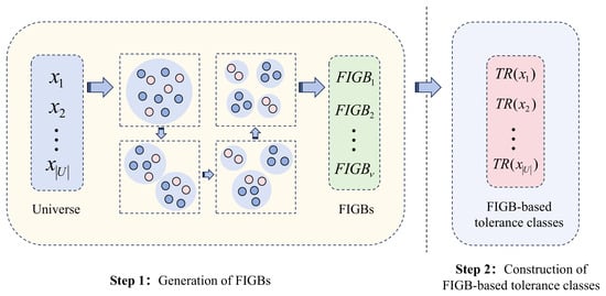
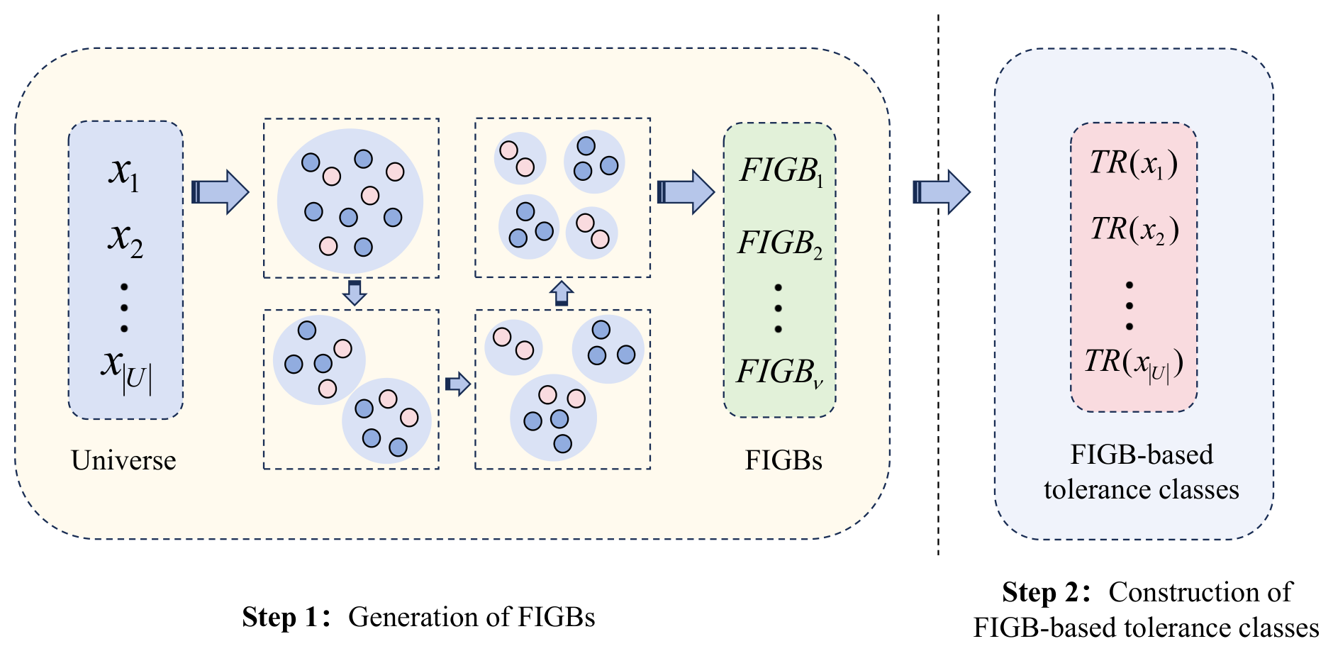
The procedure for constructing $FIGB$-based tolerance classes is illustrated in Figure 3. Step 1: We generate fuzzy interval-valued granular balls on the universe. Initially, all objects are regarded as a fuzzy interval-valued granular ball. Each object is assigned to the center with the highest membership degree. If the purity does not satisfy a given threshold, the fuzzy interval-valued granular ball is split; otherwise, it is not split. The process continues until a stable set of fuzzy interval-valued granular balls is obtained. Step 2: Tolerance classes are adaptively generated based on fuzzy interval-valued granular balls. All objects in each granular ball form a tolerance class.

Figure 3. Construction of $FIGB$-based tolerance classes.

Definition 18

([12]). In an $INDS$, the partition of $\mathcal{D}$ is defined as

$$\mathcal{U}/\mathcal{D}=\{{\mathcal{D}}_1,{\mathcal{D}}_2,\dots ,{\mathcal{D}}_{|\mathcal{U}/\mathcal{D}|}\}.$$

(22)

In rough set theory, the following property describes the relationship between $FIGB$-based tolerance classes and decision classes.

Property 1.

In an $INDS$, $\mathcal{P}\subseteq \mathcal{AT}$, ${\mathcal{D}}_d\in \mathcal{U}/\mathcal{D}$, $\forall x_h\in FIGB$, if $T\left(FIGB\right)=1$, then $T{R}_{\mathcal{P}}\left(x_h\right)\subseteq {\mathcal{D}}_d$.

Proof of Property 1. 

If $T\left(FIGB\right)=1$, then $\max |l_i|=\left|FIGB\right|$, which implies that all objects in $FIGB$ belong to the same decision class ${\mathcal{D}}_d$. Therefore, $\forall x_h\in FIGB$, we have $x_h\in {\mathcal{D}}_d$, and $FIGB\subseteq {\mathcal{D}}_d$. Since the $FIGB$-based tolerance class $T{R}_{\mathcal{P}}\left(x_h\right)$ is constructed based on the fuzzy interval-valued granular ball containing $x_h$, it follows that $T{R}_{\mathcal{P}}\left(x_h\right)\subseteq {\mathcal{D}}_d$.    □

Based on decision classes, the $FIGB$-based LA and UA in an $INDS$ are defined as follows:

Definition 19.

In an $INDS$, ${\mathcal{D}}_d\in \mathcal{U}/\mathcal{D}$, $\mathcal{P}\subseteq \mathcal{AT}$, the $FIGB$-based LA and UA are defined as

$$\underline{\mathcal{P}}\left(\mathcal{D}\right)={\displaystyle \bigcup _{d=1}^{|\mathcal{U}/\mathcal{D}|}}\underline{\mathcal{P}}\left({\mathcal{D}}_d\right),$$

(23)

$$\overline{\mathcal{P}}\left(\mathcal{D}\right)={\displaystyle \bigcup _{d=1}^{|\mathcal{U}/\mathcal{D}|}}\overline{\mathcal{P}}\left({\mathcal{D}}_d\right),$$

(24)

where $\underline{\mathcal{P}}\left({\mathcal{D}}_d\right)=\{x_h\mid x_h\in FIGB\left(\mathcal{P}\right),T{R}_{\mathcal{P}}\left(x_h\right)\subseteq {\mathcal{D}}_d\}$ is defined as the $FIGB$-based LA of ${\mathcal{D}}_d$, $\overline{\mathcal{P}}\left({\mathcal{D}}_d\right)=\{x_h\mid x_h\in FIGB\left(\mathcal{P}\right),T{R}_{\mathcal{P}}\left(x_h\right)\cap {\mathcal{D}}_d\ne ⌀\}$ is defined as the $FIGB$-based UA of ${\mathcal{D}}_d$.

In rough set theory and granular ball computing, if the $FIGB$-based tolerance class of an object is completely contained in a decision class, then the object belongs to $LA$. If the $FIGB$-based tolerance class of the object has a non-empty intersection with a decision class, then the object belongs to $UA$.

Definition 20.

In an $INDS$, $\mathcal{P}\subseteq \mathcal{AT}$, the positive region of $\mathcal{D}$ is defined as

$${\mathrm{POS}}_{\mathcal{P}}\left(\mathcal{D}\right)=\underline{\mathcal{P}}\left(\mathcal{D}\right),$$

(25)

3.2. Rank Preservation of Attribute Significance Based on FIGB

In this subsection, we investigate the rank preservation property of the attribute significance measure in an $INDS$. Based on this property, we remove redundant positive-region objects in each iteration of the reduction process to avoid unnecessary computations, thereby improving computational efficiency.

Conditional entropy measures the uncertainty of a decision attribute given conditional attributes. Therefore, it can serve as a common criterion for attribute reduction. The definition of conditional entropy is as follows:

Definition 21

([12]). In an $INDS$, ${\mathcal{D}}_d\in \mathcal{U}/\mathcal{D}$, $\mathcal{P}\subseteq \mathcal{AT}$, the conditional entropy is defined as

$$\begin{array}{cc}\hfill H\left(\mathcal{D}\right|\mathcal{P})& =-{\displaystyle \sum _{h=1}^{\left|\mathcal{U}\right|}}p\left(T{R}_{\mathcal{P}}\left(x_h\right)\right){\displaystyle \sum _{d=1}^{|\mathcal{U}/\mathcal{D}|}}p({\mathcal{D}}_d\mid T{R}_{\mathcal{P}}\left(x_h\right))logp({\mathcal{D}}_d\mid T{R}_{\mathcal{P}}\left(x_h\right))\hfill \\ \hfill & =-{\displaystyle \sum _{h=1}^{\left|\mathcal{U}\right|}}{\displaystyle \sum _{d=1}^{|\mathcal{U}/\mathcal{D}|}}{\displaystyle \frac{|T{R}_{\mathcal{P}}\left(x_h\right)\cap {\mathcal{D}}_d|}{\left|\mathcal{U}\right|}}log{\displaystyle \frac{|T{R}_{\mathcal{P}}\left(x_h\right)\cap {\mathcal{D}}_d|}{|T{R}_{\mathcal{P}}\left(x_h\right)|}},\hfill \end{array}$$

(26)

where $p\left(T{R}_{\mathcal{P}}\left(x_h\right)\right)={\displaystyle \frac{|T{R}_{\mathcal{P}}\left(x_h\right)|}{\left|\mathcal{U}\right|}}$, $p({\mathcal{D}}_d\mid T{R}_{\mathcal{P}}\left(x_h\right))={\displaystyle \frac{|T{R}_{\mathcal{P}}\left(x_h\right)\cap {\mathcal{D}}_d|}{|T{R}_{\mathcal{P}}\left(x_h\right)|}}$, and $T{R}_{\mathcal{P}}\left(x_h\right)=\{x_l\in \mathcal{U}\mid (x_h,x_l)\in I_{\mathcal{P}}\}$.

Based on conditional entropy, the definition of attribute reduction is as follows:

Definition 22

([12]). In an $INDS$, $\mathcal{P}\subseteq \mathcal{AT}$, $\forall a_k\in \mathcal{P}$, $\mathcal{P}$ is a reduct if and only if the following conditions are satisfied:

(1) 

$H(\mathcal{D}\mid \mathcal{P})=H(\mathcal{D}\mid \mathcal{AT})$;

(2) 

$H(\mathcal{D}\mid \mathcal{P})\ne H(\mathcal{D}\mid \mathcal{P}-\left\{a_k\right\})$.

Condition (1) requires that $\mathcal{P}$ has the same discriminative ability as $\mathcal{AT}$ in the $INDS$. Condition (2) ensures the independence of $\mathcal{P}$, meaning that no attribute in $\mathcal{P}$ is redundant. Therefore, a reduct contains minimal attributes while preserving the discriminative ability of the raw data.

In attribute reduction, we calculate attribute significance for selection. The definitions of two attribute significances are given as follows:

Definition 23

([12]). In an $INDS$, $\mathcal{P}\subseteq \mathcal{AT}$, $\forall a_k\in \mathcal{P}$, the internal significance of $a_k$ in $\mathcal{P}$ is defined as

$$SI{G}_{\mathrm{inner}}(a_k,\mathcal{P},\mathcal{D},\mathcal{U})=H(\mathcal{D}\mid \mathcal{P}-\left\{a_k\right\})-H(\mathcal{D}\mid \mathcal{P}).$$

(27)

If $SI{G}_{\mathrm{inner}}(a_k,\mathcal{P},\mathcal{D})>0$, then $a_k$ is a core attribute of $INDS$.

Definition 24

([12]). In an $INDS$, $\mathcal{P}\subseteq \mathcal{AT}$, $\forall a_k\in \mathcal{AT}-\mathcal{P}$, the external significance of $a_k$ in $\mathcal{P}$ is defined as

$$SI{G}_{\mathrm{outer}}(a_k,\mathcal{P},\mathcal{D},\mathcal{U})=H(\mathcal{D}\mid \mathcal{P})-H(\mathcal{D}\mid \mathcal{P}\cup \left\{a_k\right\}).$$

(28)

Based on Property 1, we have the following property.

Property 2.

In an $INDS$, $\mathcal{P}\subseteq \mathcal{AT}$, if $T\left(FIGB\right)=1$, that is, ${\mathrm{POS}}_{\mathcal{P}}\left(\mathcal{D}\right)=\{x_h\mid x_h\in FIGB\left(P\right),T{R}_{\mathcal{P}}\left(x_h\right)\subseteq {\mathcal{D}}_d\}$, then ${\displaystyle \frac{|T{R}_{\mathcal{P}}\left(x_h\right)\cap {\mathcal{D}}_d|}{\left|\mathcal{U}\right|}}log{\displaystyle \frac{|T{R}_{\mathcal{P}}\left(x_h\right)\cap {\mathcal{D}}_d|}{|T{R}_{\mathcal{P}}\left(x_h\right)|}}=0$.

Proof of Property 2. 

$\forall x_h\in FIGB$, if $T\left(FIGB\right)=1$, then all objects in the granular ball $FIGB$ have the same decision label. Based on property 1, it follows that $T{R}_{\mathcal{P}}\left(x_h\right)\subseteq {\mathcal{D}}_d$, which implies $T{R}_{\mathcal{P}}\left(x_h\right)\cap {\mathcal{D}}_d=T{R}_{\mathcal{P}}\left(x_h\right)$, where $T{R}_{\mathcal{P}}\left(x_h\right)=\{x_h\mid x_h\in FIGB\}$. Therefore, ${\displaystyle \frac{|T{R}_{\mathcal{P}}\left(x_h\right)\cap {\mathcal{D}}_d|}{\left|\mathcal{U}\right|}}log{\displaystyle \frac{|T{R}_{\mathcal{P}}\left(x_h\right)\cap {\mathcal{D}}_d|}{|T{R}_{\mathcal{P}}\left(x_h\right)|}}={\displaystyle \frac{|T{R}_{\mathcal{P}}\left(x_h\right)|}{\left|\mathcal{U}\right|}}log{\displaystyle \frac{|T{R}_{\mathcal{P}}\left(x_h\right)|}{|T{R}_{\mathcal{P}}\left(x_h\right)|}}=0$. This completes the proof.    □

To remove unnecessary positive-region objects during the iterative process of reduction, following FSPA [40], we present the proof of the rank preservation theorem of attribute significance measures based on $FIGB$.

Theorem 1.

In an $INDS$, $\mathcal{P}\subseteq \mathcal{AT}$, ${\mathcal{U}}^{\prime }=\mathcal{U}-{\mathrm{POS}}_{\mathcal{P}}\left(\mathcal{D}\right)$. $\forall a_k,a_s\in \mathcal{AT}-\mathcal{P}$, if $SI{G}_{outer}(a_k,\mathcal{P},\mathcal{D},\mathcal{U})\ge SI{G}_{outer}(a_s,\mathcal{P},\mathcal{D},\mathcal{U})$, then $SI{G}_{outer}(a_k,\mathcal{P},\mathcal{D},{\mathcal{U}}^{\prime })\ge SI{G}_{outer}(a_s,\mathcal{P},\mathcal{D},{\mathcal{U}}^{\prime })$.

Proof of Theorem 1. 

$T{R}_{\mathcal{P}}=\{T{R}_{\mathcal{P}}\left(x_h\right)\mid h=1,2,\dots ,t,t+1,\dots ,\left|\mathcal{U}\right|\}$ and $\mathcal{U}/\mathcal{D}=\{{\mathcal{D}}_1,{\mathcal{D}}_2,\dots ,{\mathcal{D}}_{|\mathcal{U}/\mathcal{D}|}\}$, ${\mathcal{D}}_d\in \mathcal{U}/\mathcal{D}$, where $T{R}_{\mathcal{P}}\left(x_{t+1}\right),\dots ,T{R}_{\mathcal{P}}\left(x_{\left|\mathcal{U}\right|}\right)\subseteq {\mathrm{POS}}_{\mathcal{P}}\left(\mathcal{D}\right)$. Then

$$\begin{array}{cc}& H^{\mathcal{U}}\left(\mathcal{D}\right|\mathcal{P})=-{\displaystyle \sum _{h=1}^{\left|\mathcal{U}\right|}}{\displaystyle \sum _{d=1}^{|\mathcal{U}/\mathcal{D}|}}{\displaystyle \frac{|T{R}_{\mathcal{P}}\left(x_h\right)\cap {\mathcal{D}}_d|}{\left|\mathcal{U}\right|}}log{\displaystyle \frac{|T{R}_{\mathcal{P}}\left(x_h\right)\cap {\mathcal{D}}_d|}{|T{R}_{\mathcal{P}}\left(x_h\right)|}}\hfill \\ \hfill & =-\left({\displaystyle \sum _{h=1}^t}{\displaystyle \sum _{d=1}^{|\mathcal{U}/\mathcal{D}|}}{\displaystyle \frac{|T{R}_{\mathcal{P}}\left(x_h\right)\cap {\mathcal{D}}_d|}{\left|\mathcal{U}\right|}}log{\displaystyle \frac{|T{R}_{\mathcal{P}}\left(x_h\right)\cap {\mathcal{D}}_d|}{|T{R}_{\mathcal{P}}\left(x_h\right)|}}+{\displaystyle \sum _{h=t+1}^{\left|\mathcal{U}\right|}}{\displaystyle \sum _{d=1}^{|\mathcal{U}/\mathcal{D}|}}{\displaystyle \frac{|T{R}_{\mathcal{P}}\left(x_h\right)|}{\left|\mathcal{U}\right|}}log{\displaystyle \frac{|T{R}_{\mathcal{P}}\left(x_h\right)|}{|T{R}_{\mathcal{P}}\left(x_h\right)|}}\right)\hfill \\ \hfill & =-{\displaystyle \sum _{h=1}^t}{\displaystyle \sum _{d=1}^{|\mathcal{U}/\mathcal{D}|}}{\displaystyle \frac{|T{R}_{\mathcal{P}}\left(x_h\right)\cap {\mathcal{D}}_d|}{\left|\mathcal{U}\right|}}log{\displaystyle \frac{|T{R}_{\mathcal{P}}\left(x_h\right)\cap {\mathcal{D}}_d|}{|T{R}_{\mathcal{P}}\left(x_h\right)|}}\hfill \\ \hfill & =-{\displaystyle \frac{|{\mathcal{U}}^{\prime }|}{\left|\mathcal{U}\right|}}{\displaystyle \sum _{h=1}^t}{\displaystyle \sum _{d=1}^{|\mathcal{U}/\mathcal{D}|}}{\displaystyle \frac{|T{R}_{\mathcal{P}}\left(x_h\right)\cap {\mathcal{D}}_d|}{|{\mathcal{U}}^{\prime }|}}log{\displaystyle \frac{|T{R}_{\mathcal{P}}\left(x_h\right)\cap {\mathcal{D}}_d|}{|T{R}_{\mathcal{P}}\left(x_h\right)|}}\hfill \\ \hfill & ={\displaystyle \frac{|{\mathcal{U}}^{\prime }|}{\left|\mathcal{U}\right|}}{H}^{{\mathcal{U}}^{\prime }}\left(\mathcal{D}\right|\mathcal{P}),\hfill \end{array}$$

(29)

$$\begin{array}{cc}& H^{\mathcal{U}}\left(\mathcal{D}\right|\mathcal{P}\cup \left\{a_k\right\})=-{\displaystyle \sum _{h=1}^{\left|\mathcal{U}\right|}}{\displaystyle \sum _{d=1}^{|\mathcal{U}/\mathcal{D}|}}{\displaystyle \frac{|T{R}_{\mathcal{P}\cup \left\{a_k\right\}}\left(x_h\right)\cap {\mathcal{D}}_d|}{\left|\mathcal{U}\right|}}log{\displaystyle \frac{|T{R}_{\mathcal{P}\cup \left\{a_k\right\}}\left(x_h\right)\cap {\mathcal{D}}_d|}{|T{R}_{\mathcal{P}\cup \left\{a_k\right\}}\left(x_h\right)|}}\hfill \\ \hfill & =-({\displaystyle \sum _{h=1}^t}{\displaystyle \sum _{d=1}^{|\mathcal{U}/\mathcal{D}|}}{\displaystyle \frac{|T{R}_{\mathcal{P}\cup \left\{a_k\right\}}\left(x_h\right)\cap {\mathcal{D}}_d|}{\left|\mathcal{U}\right|}}log{\displaystyle \frac{|T{R}_{\mathcal{P}\cup \left\{a_k\right\}}\left(x_h\right)\cap {\mathcal{D}}_d|}{|T{R}_{\mathcal{P}\cup \left\{a_k\right\}}\left(x_h\right)|}}\hfill \\ \hfill & +{\displaystyle \sum _{h=t+1}^{\left|\mathcal{U}\right|}}{\displaystyle \sum _{d=1}^{|\mathcal{U}/\mathcal{D}|}}{\displaystyle \frac{|T{R}_{\mathcal{P}\cup \left\{a_k\right\}}\left(x_h\right)|}{\left|\mathcal{U}\right|}}log{\displaystyle \frac{|T{R}_{\mathcal{P}\cup \left\{a_k\right\}}\left(x_h\right)|}{|T{R}_{\mathcal{P}\cup \left\{a_k\right\}}\left(x_h\right)|}})\hfill \\ \hfill & =-{\displaystyle \sum _{h=1}^t}{\displaystyle \sum _{d=1}^{|\mathcal{U}/\mathcal{D}|}}{\displaystyle \frac{|T{R}_{\mathcal{P}\cup \left\{a_k\right\}}\left(x_h\right)\cap {\mathcal{D}}_d|}{\left|\mathcal{U}\right|}}log{\displaystyle \frac{|T{R}_{\mathcal{P}\cup \left\{a_k\right\}}\left(x_h\right)\cap {\mathcal{D}}_d|}{|T{R}_{\mathcal{P}\cup \left\{a_k\right\}}\left(x_h\right)|}}\hfill \\ \hfill & =-{\displaystyle \frac{|{\mathcal{U}}^{\prime }|}{\left|\mathcal{U}\right|}}{\displaystyle \sum _{h=1}^t}{\displaystyle \sum _{d=1}^{|\mathcal{U}/\mathcal{D}|}}{\displaystyle \frac{|T{R}_{\mathcal{P}\cup \left\{a_k\right\}}\left(x_h\right)\cap {\mathcal{D}}_d|}{|{\mathcal{U}}^{\prime }|}}log{\displaystyle \frac{|T{R}_{\mathcal{P}\cup \left\{a_k\right\}}\left(x_h\right)\cap {\mathcal{D}}_d|}{|T{R}_{\mathcal{P}\cup \left\{a_k\right\}}\left(x_h\right)|}}\hfill \\ \hfill & ={\displaystyle \frac{|{\mathcal{U}}^{\prime }|}{\left|\mathcal{U}\right|}}{H}^{{\mathcal{U}}^{\prime }}\left(\mathcal{D}\right|\mathcal{P}\cup \left\{a_k\right\}),\hfill \end{array}$$

(30)

$$\begin{array}{cc}& SI{G}_{\mathrm{outer}}(a_k,\mathcal{P},\mathcal{D},\mathcal{U})=H^{\mathcal{U}}(\mathcal{D}\mid \mathcal{P})-H^{\mathcal{U}}(\mathcal{D}\mid \mathcal{P}\cup \left\{a_k\right\})\hfill \\ \hfill & ={\displaystyle \frac{|{\mathcal{U}}^{\prime }|}{\left|\mathcal{U}\right|}}{H}^{{\mathcal{U}}^{\prime }}(\mathcal{D}\mid \mathcal{P})-{\displaystyle \frac{|{\mathcal{U}}^{\prime }|}{\left|\mathcal{U}\right|}}{H}^{{\mathcal{U}}^{\prime }}(\mathcal{D}\mid \mathcal{P}\cup \left\{a_k\right\})\hfill \\ \hfill & ={\displaystyle \frac{|{\mathcal{U}}^{\prime }|}{\left|\mathcal{U}\right|}}(H^{{\mathcal{U}}^{\prime }}(\mathcal{D}\mid \mathcal{P})-H^{{\mathcal{U}}^{\prime }}(\mathcal{D}\mid \mathcal{P}\cup \left\{a_k\right\}))\hfill \\ \hfill & ={\displaystyle \frac{|{\mathcal{U}}^{\prime }|}{\left|\mathcal{U}\right|}}SI{G}_{\mathrm{outer}}(a_k,\mathcal{P},\mathcal{D},{\mathcal{U}}^{\prime })\hfill \end{array}$$

(31)

$\forall a_k,a_s\in \mathcal{AT}-\mathcal{P}$, we obtain $SI{G}_{\mathrm{outer}}(a_k,\mathcal{P},\mathcal{D},{\mathcal{U}}^{\prime })={\displaystyle \frac{\left|\mathcal{U}\right|}{|{\mathcal{U}}^{\prime }|}}SI{G}_{\mathrm{outer}}(a_k,\mathcal{P},\mathcal{D},\mathcal{U})$, $SI{G}_{\mathrm{outer}}(a_s,\mathcal{P},\mathcal{D},{\mathcal{U}}^{\prime })={\displaystyle \frac{\left|\mathcal{U}\right|}{|{\mathcal{U}}^{\prime }|}}SI{G}_{\mathrm{outer}}(a_s,\mathcal{P},\mathcal{D},\mathcal{U})$. If $SI{G}_{\mathrm{outer}}(a_k,\mathcal{P},\mathcal{D},\mathcal{U})\ge$ $SI{G}_{\mathrm{outer}}(a_s,\mathcal{P},\mathcal{D},\mathcal{U})$, then $SI{G}_{\mathrm{outer}}(a_k,\mathcal{P},\mathcal{D},{\mathcal{U}}^{\prime })\ge SI{G}_{\mathrm{outer}}(a_s,\mathcal{P},\mathcal{D},{\mathcal{U}}^{\prime })$.    □

According to Theorem 1, in both the universe $\mathcal{U}$ and the reduced universe ${\mathcal{U}}^{\prime }$, the ranking of attribute significance remains unchanged. Thus, in each iteration, we can compute attribute significance on the reduced universe, which decreases the computational cost and enhances the efficiency of the reduction process. This theorem provides the theoretical foundation for the design of the heuristic reduction algorithm in the next section.

4. Algorithms via Fuzzy Granular Balls for Interval-Valued Decision Systems

Based on the fuzzy interval-valued granular balls in the previous section, this section presents an algorithm for constructing $FIGB$-based tolerance classes. Furthermore, an efficient attribute reduction algorithm is proposed based on the $FIGB$-based tolerance classes and the positive region acceleration method.

Algorithm 1 constructs tolerance classes based on FIGB for interval-valued decision systems.

At the beginning of Algorithm 1, $\mathcal{U}$ is regarded as the initial fuzzy interval-valued granular ball. This fuzzy interval-valued granular ball has minimal purity and is therefore unable to reflect the data distribution. Each $FIGB\in RGBs$ is iteratively checked for purity. If $T\left(FIGB\right)\ge \delta$, $FIGB$ is stable and added to $NGBs$. Otherwise, $FIGB$ is further split. In this case, based on the random seed, $k-1$ heterogeneous objects are randomly selected from $FIGB$ as new centers. The membership degrees are calculated, and objects are assigned to the centers with the highest membership degrees. Then $FIGB$ is split into k finer granular balls. All newly generated granular balls are collected into $NGBs$. This splitting procedure is repeated until the number of granular balls remains unchanged, indicating that the granular ball structure is stable and no further refinement is required. As the algorithm proceeds, the purity of granular balls gradually increases, and the decision boundaries become distinct. Eventually, a stable set of fuzzy interval-valued granular balls is obtained. We subsequently compute each object’s tolerance class. During the FIGB generation process, the number of objects processed in each iteration does not exceed $\mathcal{U}$. Each object is calculated with k centers.

Algorithm 1: FIGB-based tolerance class construction algorithm for interval-valued decision systems (TFIGB).

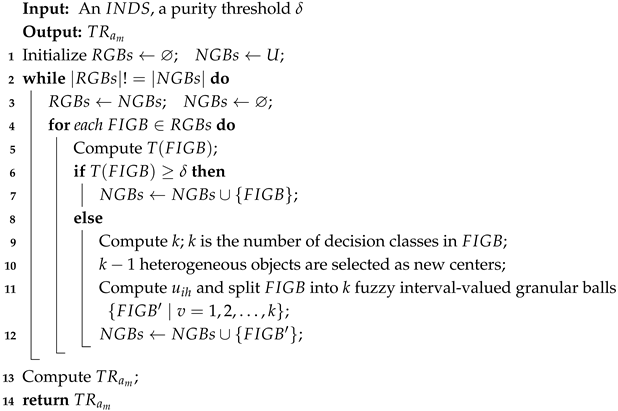The time complexity of Algorithm 1 is $O\left(\right|\mathcal{U}\left|kt\right)$, where $\left|\mathcal{U}\right|$ is the number of objects, k is the number of decision classes, and t is the number of iterations.

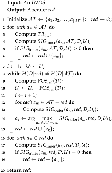
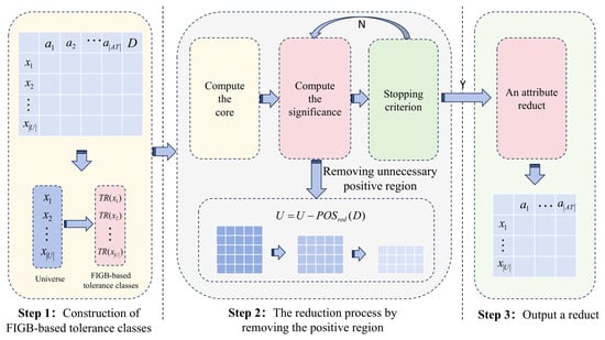
Based on Theorem 1, we present a fast approximate attribute reduction algorithm via fuzzy granular balls for interval-valued decision systems (FRFIGB). Figure 4 illustrates the procedure of FRFIGB. Step 1: Fuzzy interval-valued granular balls are used to rapidly and adaptively construct tolerance classes for each object. Step 2: During each iteration of attribute significance computation, redundant objects in the positive region are removed, thereby decreasing the computational time. Step 3: The reduction result is output.

Figure 4. The reduction process of FRFIGB.

As shown in Algorithm 2, FRFIGB is divided into three parts. In the first part (Steps 1–6), the $FIGB$-based tolerance classes corresponding to each attribute are computed. The internal significance of each attribute is evaluated, and attributes that satisfy the condition are added to the candidate set. The time complexity of this part is $O\left(\right|\mathcal{AT}{|}^2\left|\mathcal{U}\right|kt)$. In the second part (Steps 7–15), if the conditional entropy of the candidate set differs from the attribute set $\mathcal{AT}$, the current positive region of the candidate set is computed. Objects that already belong to the positive region are removed from $\mathcal{U}$, and the updated ${\mathcal{U}}_i$ is used in the next iterations. The attribute with the highest external significance is iteratively added to the candidate set until the constraint is satisfied. The time complexity of the second stage is $O\left({\sum }_{i=1}^{\left|\mathcal{AT}\right|}{\left|\mathcal{AT}\right|}^2\left|{\mathcal{U}}_i\right|\right)$. In the last part (Steps 16–20), unnecessary attributes are removed from the candidate set. Therefore, the time complexity is approximately ${O\left(\right|\mathcal{AT}|}^2\left|\mathcal{U}\right|kt)+O\left({\sum }_{i=1}^{\left|\mathcal{AT}\right|}{\left|\mathcal{AT}\right|}^2\left|{\mathcal{U}}_i\right|\right)$.

Algorithm 2: A fast approximate attribute reduction algorithm via fuzzy granular balls for interval-valued decision systems (FRFIGB).

5. Experimental Analyses

To evaluate the effectiveness of TFIGB and FRFIGB, a series of comparative experiments is conducted and discussed in this section. The experiments include: (1) Comparison of tolerance class construction time; (2) Comparison of attribute reduction time; (3) Ablation study; (4) Comparison of classification accuracy; (5) Sensitivity analysis; (6) Comparison of the number of selected attributes. The experiments are conducted on a computer with the Windows 11 (64-bit) operating system and an Intel Core i5-13500H CPU. The program environment consists of PyCharm 2023.3.2 and Python 3.9. The ten datasets used in the experiments are obtained from the UCI Machine Learning Repository (https://archive-beta.ics.uci.edu/). The details of the ten UCI datasets are shown in Table 2.

Table 2. UCI datasets.

No.	Dataset	Abbr.	$\left|\mathcal{U}\right|$	$\left|\mathcal{AT}\right|$	$\left|\mathcal{D}\right|$
1	Soybean	Soyb	683	35	3
2	Breast_cancer_wisconsin	Brea	699	9	2
3	TCGA_infowithgrade	Tiwg	839	23	2
4	German	Germ	1000	20	2
5	Drug_consumption	Drug	1885	12	7
6	Faults	Faul	1941	27	2
7	Wifi_localization	Wifi	2000	7	4
8	Rice_cammeo_osmancik	Rice	3810	7	2
9	Online_shoppers_intention	Line	12,330	17	2
10	default_of_credit_card_clients	Defa	30,000	23	2

In Table 2, $\left|\mathcal{U}\right|$ and $\left|\mathcal{AT}\right|$ denote the numbers of objects and conditional attributes, respectively, and $\left|\mathcal{D}\right|$ denotes the number of decision classes.

In the above datasets, numerical encoding is applied: missing data are replaced by high-frequency values in the same condition attribute; nominal data are encoded using 0, 1; and continuous data are discretized using an equal-frequency partitioning method. Based on [41], the formula for the interval number transformation is defined as follows

$$m_h^k=a_k\left(x_h\right)-2{\theta }_t,$$

(32)

$$n_h^k=a_k\left(x_h\right)+2{\theta }_t,$$

(33)

where ${\theta }_t$ denotes the standard deviation of the corresponding attribute, and its calculation formula is

$${\theta }_t=\sqrt{{\displaystyle \frac{1}{\left|U\right|}}\sum _{x_h\in \mathcal{U}}{\left(a_k\left(x_h\right)-ave\left(a_k\right)\right)}^2},$$

(34)

$$ave\left(a_k\right)={\displaystyle \frac{1}{\left|U\right|}}\sum _{x_h\in \mathcal{U}}{a}_k\left(x_h\right),$$

(35)

where $a_k\left(x_h\right)$ represents the value of object $x_h$ on attribute $a_k$, $ave\left(a_k\right)$ represents the mean value of attribute $a_k$.

FRFIGB is compared with ARIE [11], ARCE [12], ARRE [13], FSPA [40], FH-IU-AR [42] and CH-HSD-AR [42]. FSPA and ARCE adopt the same similarity degree calculation formula. The interval-valued similarity degree threshold is 0.8.

Based on existing studies, when the purity threshold lies within $[0.90,1.00]$, the reduct can achieve high classification accuracy and exhibit good robustness to noise; thus, $\delta$ is set to $0.95$. In all algorithms, redundant attributes are removed from the reducts. In existing studies, the purity threshold is usually set within $[0.90,1.00]$. In this study, we set $\delta =0.95$.

5.1. Comparison of Tolerance Class Construction Time

In this subsection, we compare the computational time of tolerance class construction. Table 3 shows the computational time required for tolerance class construction by six algorithms. In Table 3, the best result in each row is shown in bold. It can be observed that TFIGB has the shortest computational time on all datasets. On the Tiwg dataset, TFIGB, ARIE, ARCE, ARRE, FH-IU-AR, and CH-HSD-AR take 1.61 s, 24.44 s, 33.81 s, 34.27 s, 14.63 s, and 14.09 s, respectively. On average, TFIGB takes 110.40 s, whereas the average running times of ARIE, ARCE, ARRE, FH-IU-AR, and CH-HSD-AR are 3768.11 s, 3682.21 s, 3910.38 s, 2218.94 s, and 2676.27 s, respectively.

Table 3. Comparison of $FIGB$-based tolerance class construction time (s).

No.	Abbr.	ARIE	ARCE	ARRE	FH-IU-AR	CH-HSD-AR	TFIGB
1	Soyb	22.76	30.08	28.59	14.97	14.06	2.76
2	Brea	7.14	9.19	9.66	4.18	3.91	0.60
3	Tiwg	24.44	33.81	34.27	14.63	14.09	1.61
4	Germ	32.12	41.33	45.09	22.21	17.77	2.16
5	Drug	70.70	74.55	81.46	41.53	36.51	15.23
6	Faul	214.71	220.90	212.91	91.86	117.53	21.54
7	Wifi	46.96	52.18	54.78	32.19	29.43	4.13
8	Rice	171.52	206.39	224.42	124.54	114.68	14.20
9	Line	6403.54	6732.17	7445.31	3137.82	2116.04	207.15
10	Defa	30,687.23	29,421.45	30,967.34	18,705.49	24,298.65	834.64
	Avg	3768.11	3682.21	3910.38	2218.94	2676.27	110.40

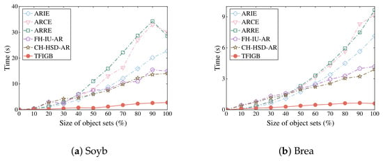
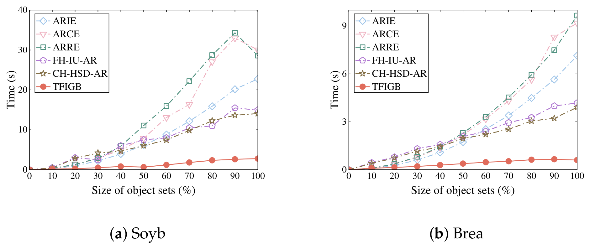
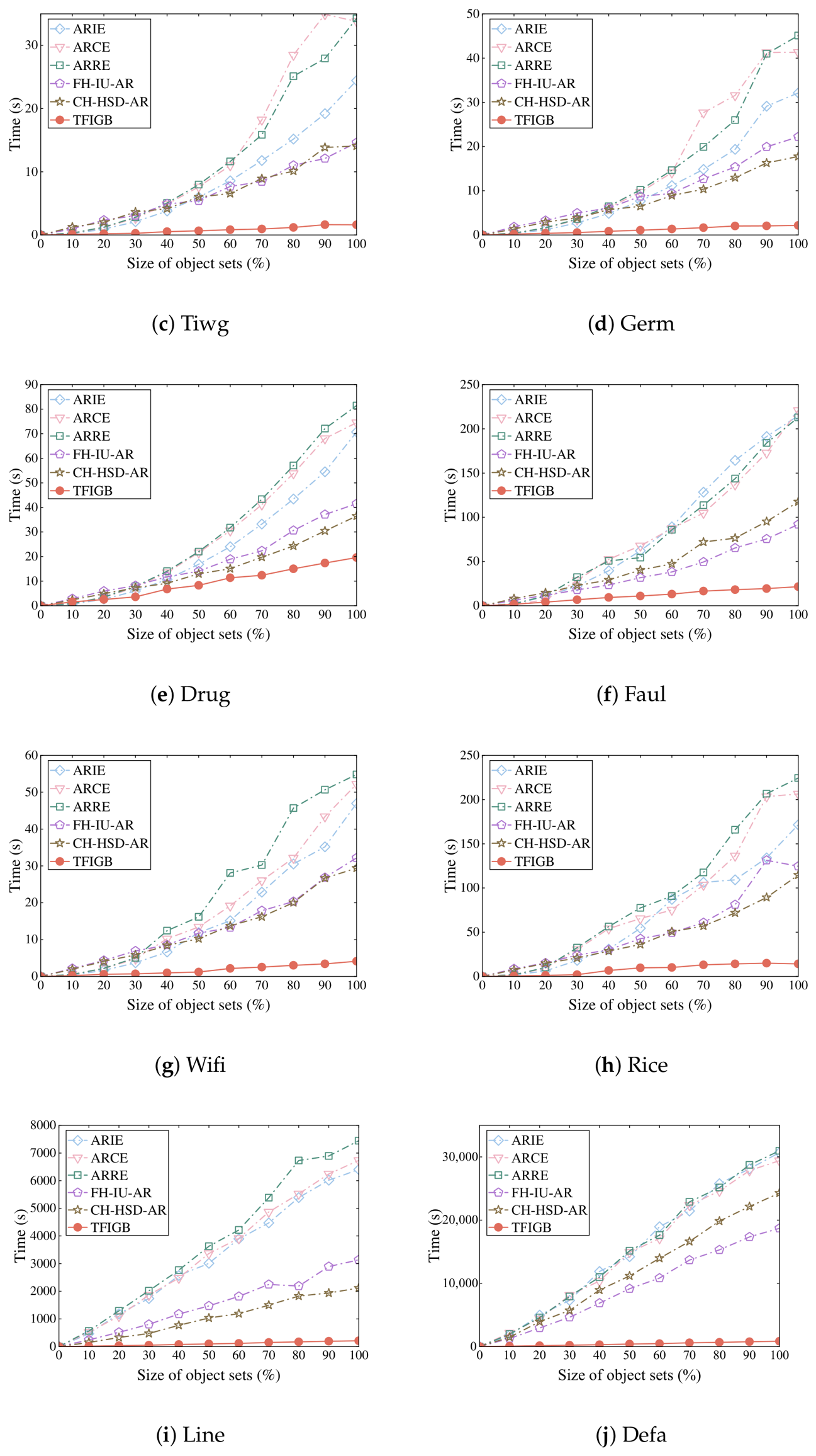
Figure 5 shows the trend in tolerance class construction time for six algorithms (ARIE, ARCE, ARRE, FH-IU-AR, CH-HSD-AR, and TFIGB) as the size of the object sets increases. The horizontal axis corresponds to the size of the objects used, and the vertical axis reports the time required to construct tolerance classes. For evaluation, the object set is split into ten subsets, and the running time is measured on 10%, 20%, …, up to 100% of the whole object set. The running time of all approaches increases as the number of objects grows, while that of TFIGB increases much more slowly. For example, on the Soyb dataset, as the size of the object sets increases from 40% to 90%, the running time rises from 3.80 s to 19.99 s for ARIE, the running time rises from 4.65 s to 32.17 s for ARCE, the running time rises from 6.01 s to 33.71 s for ARRE, the running time rises from 5.98 s to 15.47 s for FH-IU-AR, and the running time rises from 4.62 s to 13.65 s for CH-HSD-AR, while TFIGB increases from 0.76 s to 2.31 s.

Figure 5. Comparison of tolerance class construction time with increasing size of the object sets.

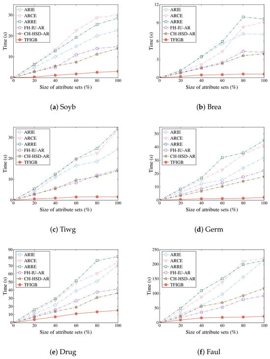
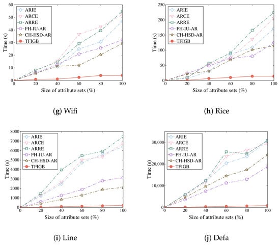
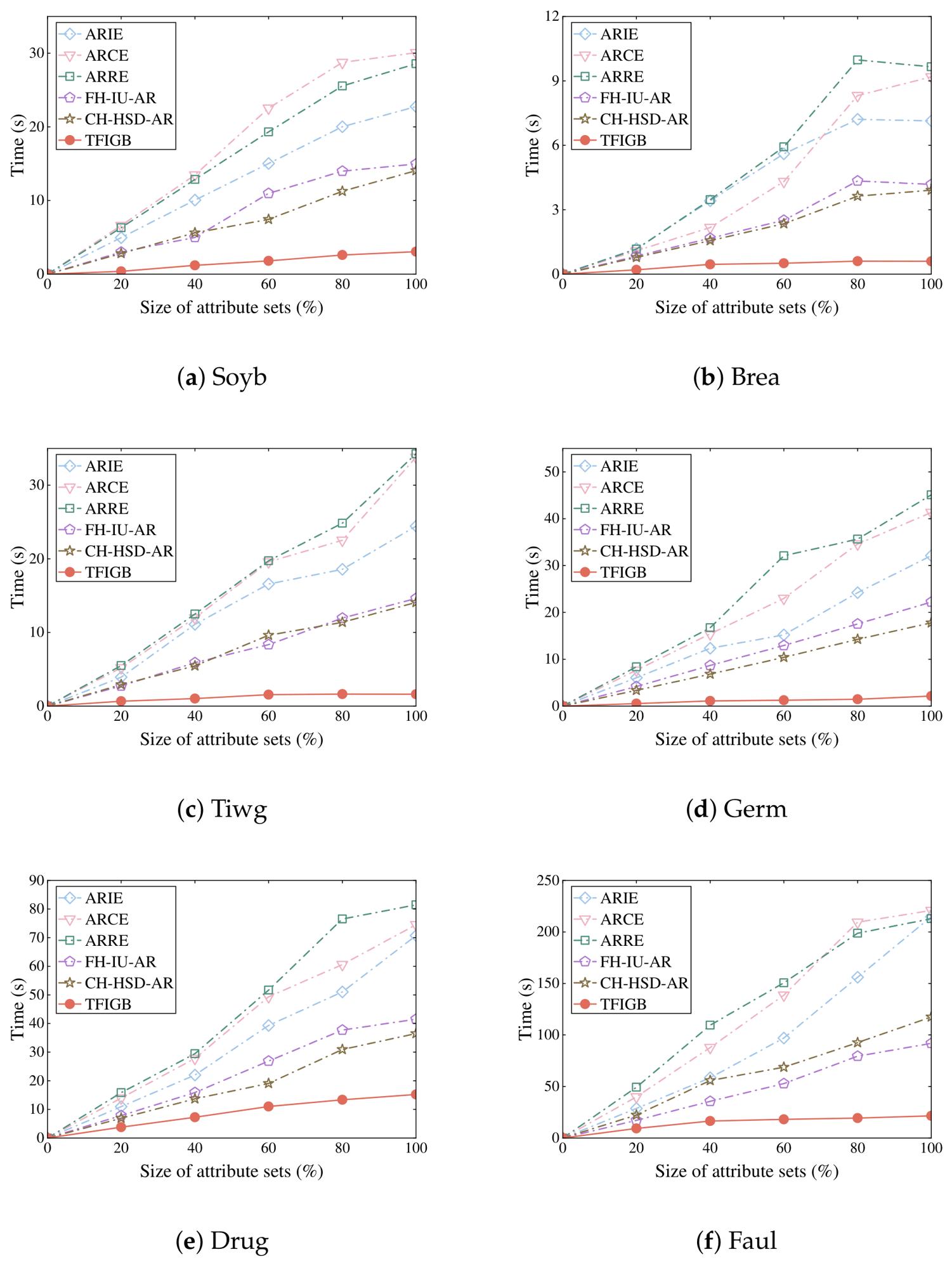
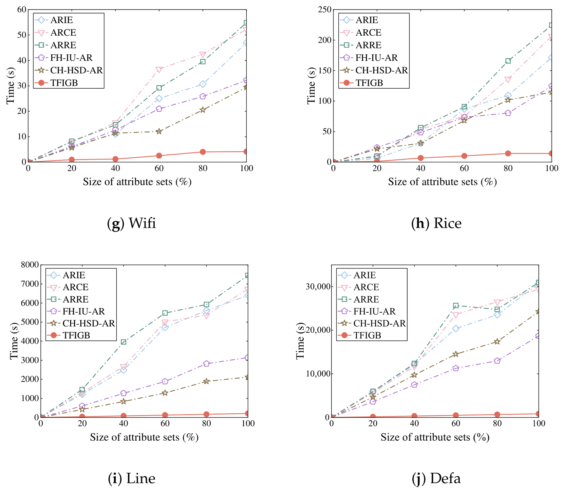
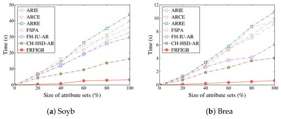
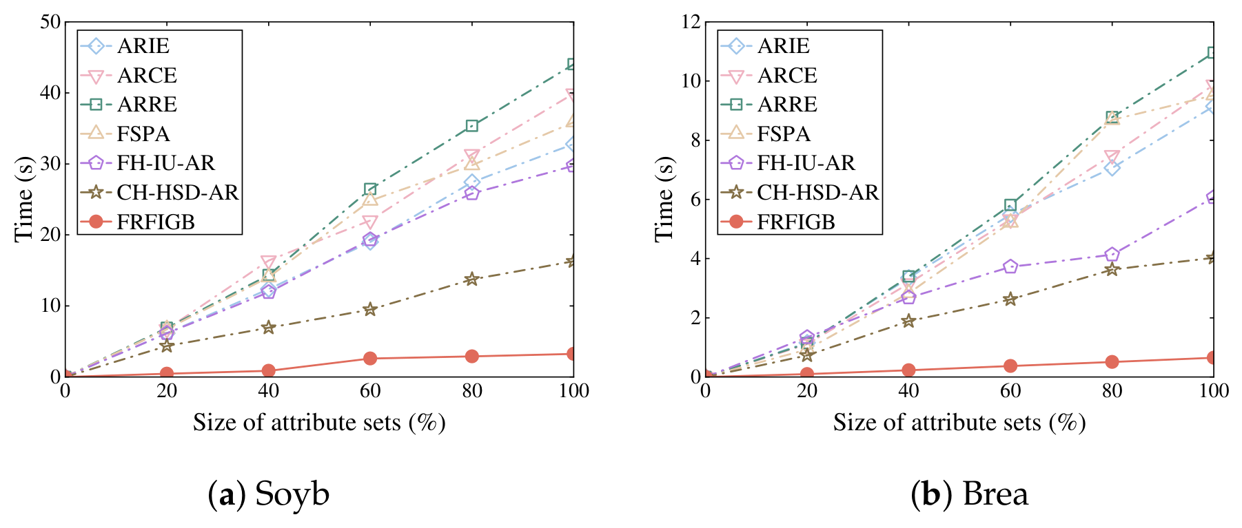
The trend of tolerance class construction time as the attribute sets change is illustrated in Figure 6. The horizontal axis and vertical axis represent the size of attribute sets and the time required to construct tolerance classes, respectively. The attribute set is divided into five subsets, and time comparisons are conducted on 20%, 40%, …, up to 100% of the whole attribute set. As shown in the subfigures, TFIGB has the shortest running time on all datasets for the same number of attributes. For example, on the Tiwg dataset, when the size of attribute sets is 60%, the tolerance class construction times of ARIE, ARCE, ARRE, FH-IU-AR, and CH-HSD-AR are 8.57 s, 11.01 s, 11.03 s, 7.68 s, and 6.57 s, respectively, whereas TFIGB takes 0.82 s. When the size of attribute sets is 80%, the tolerance class construction times of ARIE, ARCE, ARRE, FH-IU-AR, and CH-HSD-AR are 15.17 s, 28.49 s, 25.13 s, 11.02 s, and 10.11 s, respectively, whereas TFIGB takes 1.19 s. In other words, TFIGB takes the shortest time when processing attribute sets with the same number of attributes.

Figure 6. Comparison of tolerance class construction time with increasing size of attribute sets.

5.2. Comparison of Attribute Reduction Time

To validate the efficiency of the proposed algorithm FRFIGB, this subsection compares the attribute reduction time of seven algorithms (ARIE, ARCE, ARRE, FSPA, FH-IU-AR, CH-HSD-AR, and FRFIGB).

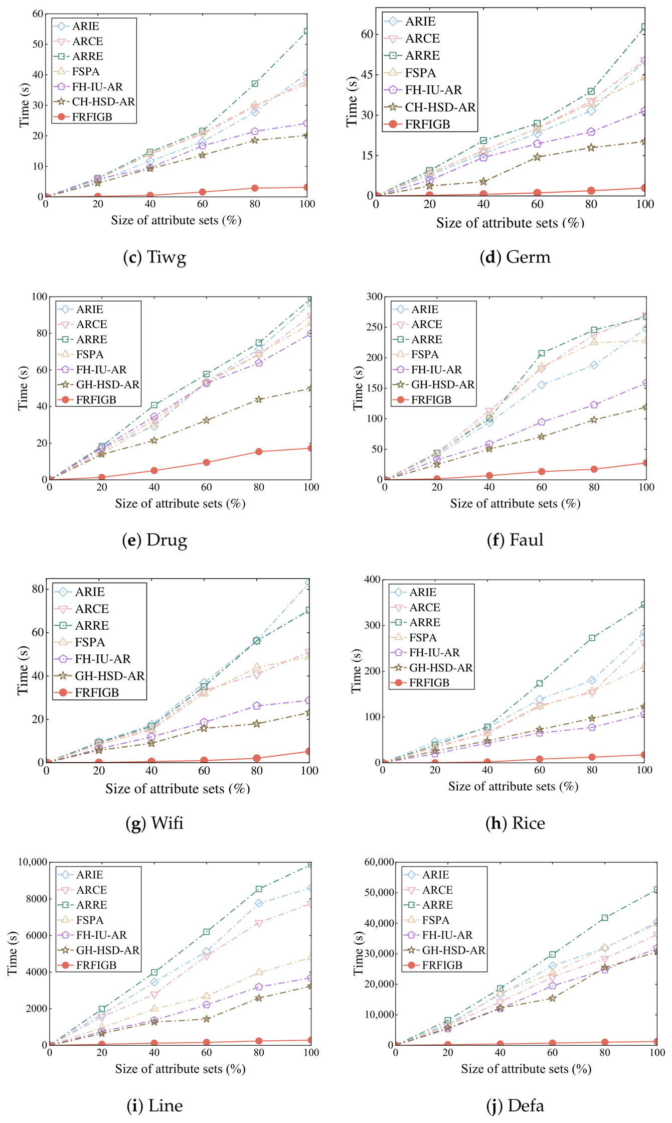
As shown in Table 4, FRFIGB has the shortest attribute reduction time on all datasets. On the Brea dataset, FRFIGB takes 0.65 s. In comparison, the corresponding times for ARIE, ARCE, ARRE, FSPA, FH-IU-AR, and CH-HSD-AR are 9.15 s, 9.88 s, 10.96 s, 9.52 s, 6.07 s, and 4.03 s, respectively. The average reduction time of FRFIGB is 162.51 s, whereas the average reduction time of the comparison algorithms ranges from 3425.50 s to 6193.76 s. FRFIGB is approximately 21.08–38.11 times faster than the other algorithms.

Table 4. Comparison of attribute reduction time (s).

No.	Abbr.	ARIE	ARCE	ARRE	FSPA	FH-IU-AR	CH-HSD-AR	FRFIGB
1	Soyb	32.81	39.92	44.03	35.88	29.75	16.29	3.25
2	Brea	9.15	9.88	10.96	9.52	6.07	4.03	0.65
3	Tiwg	40.52	38.01	54.30	36.98	24.12	20.15	3.12
4	Germ	50.23	50.58	62.85	44.03	31.7	20.23	2.95
5	Drug	96.55	89.77	99.06	85.59	79.96	50.02	17.30
6	Faul	248.35	270.43	266.95	228.12	158.75	119.26	27.80
7	Wifi	83.12	51.23	70.45	48.97	28.75	23.13	5.23
8	Rice	285.60	262.18	345.93	210.45	106.11	122.96	17.50
9	Line	8601.40	7753.87	9886.14	4799.87	3692.96	3235.16	289.26
10	Defa	40,368.50	36,390.80	51,096.94	39,854.05	31,913.05	30,643.76	1258.01
	Avg	4981.62	4495.67	6193.76	4535.35	3607.12	3425.50	162.51

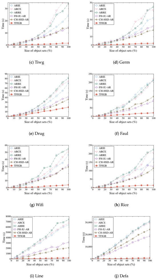
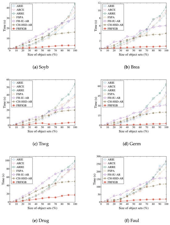
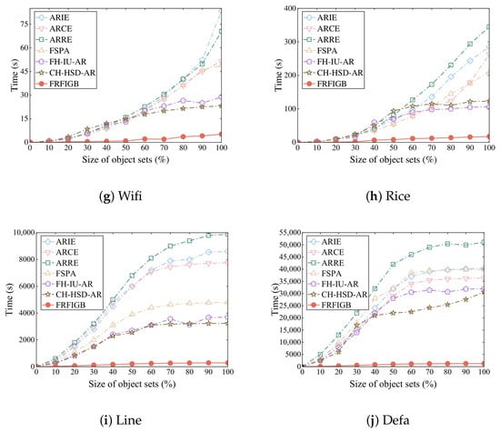
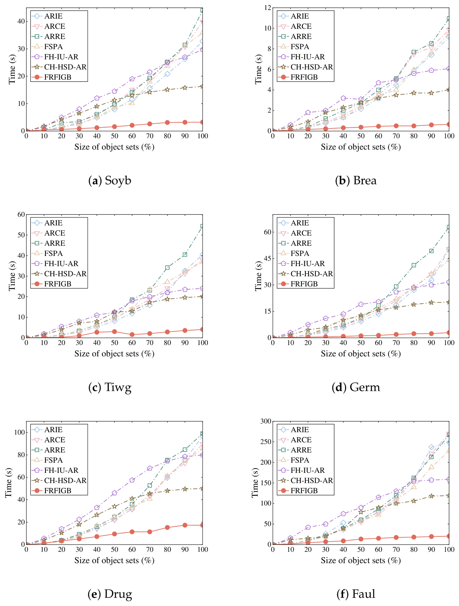
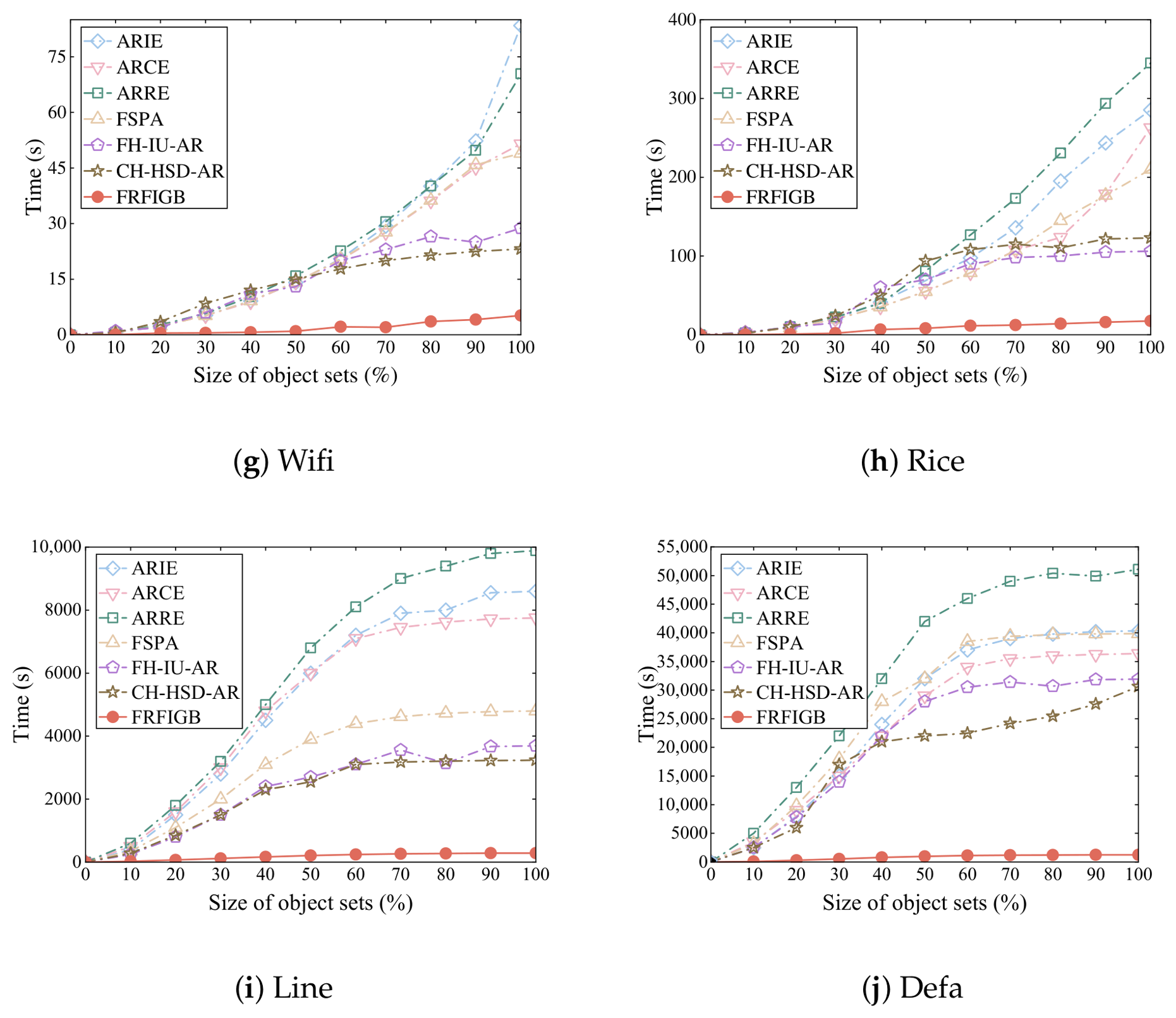
Figure 7 shows the trend in reduction time as the size of the object sets increases on different datasets and algorithms. For each subfigure in Figure 7, the horizontal axis corresponds to the size of the objects used, and the vertical axis denotes the reduction time. The object set is sampled at 10%, 20%, …, up to 100% of the entire object set for computation. FRFIGB has the shortest running time on all datasets for the same size of the object sets. For example, on the Drug dataset, when the object set size is 70%, the reduction times of ARIE, ARCE, ARRE, FSPA, FH-IU-AR, and CH-HSD-AR are 43.10 s, 44.01 s, 55.39 s, 41.07 s, 68.21 s, and 45.50 s, respectively, whereas FRFIGB takes 11.31 s. When the object set size is 90%, the reduction times of ARIE, ARCE, ARRE, FSPA, FH-IU-AR, and CH-HSD-AR are 76.51 s, 70.81 s, 89.75 s, 71.09 s, 78.50 s, and 49.50 s, respectively, whereas FRFIGB takes 16.27 s.

Figure 7. Comparison of attribute reduction time with increasing size of the object sets.

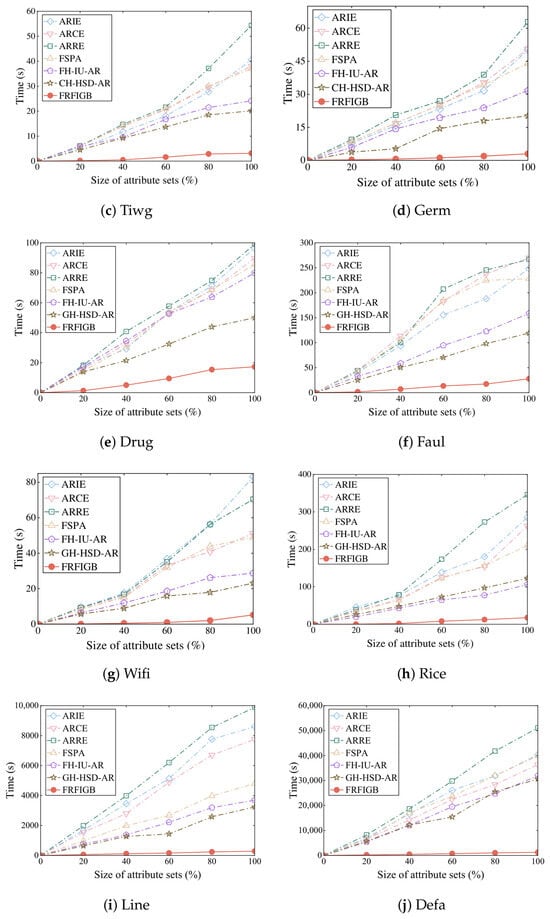
The trend of reduction time as the attribute sets change is shown in Figure 8. The horizontal axis and vertical axis represent the size of attribute sets and the reduction time, respectively. The attribute set is sampled at 20%, 40%, …, up to 100% of the whole attribute set for computation. This shows the relationship between the size of attribute sets and the reduction time of each algorithm. As the attribute subset grows, FRFIGB shows a mild increase in running time. For example, on the Defa dataset, as the size of attribute sets increases from 20% to 100%, the running time rises from 7017.88 s to 40,368.50 s for ARIE, the running time rises from 6557.43 s to 36,390.80 s for ARCE, the running time rises from 8241.76 s to 51,096.94 s for ARRE, the running time rises from 6407.94 s to 39,854.05 s for FSPA, the running time rises from 5418.10 s to 31,913.05 s for FH-IU-AR, the running time rises from 5694.35 s to 30,643.76 s for CH-HSD-AR, while FRFIGB increases from 226.94 s to 1258.01 s.

Figure 8. Comparison of attribute reduction time with increasing size of attribute sets.

5.3. Ablation Study

To investigate the contributions of different components in FRFIGB, an ablation study is conducted in this subsection. Table 5 shows the ablation results of FIGB construction and the positive-region acceleration strategy on reduction time. The results show that FRFIGB achieves the highest running efficiency on all datasets when both FIGB construction and positive-region acceleration are used together. “✓” indicates used; “×” indicates not used.

Table 5. Ablation study of the effects of FIGB construction and positive-region acceleration on reduction time (s).

FIGB	Positive-Region Acceleration	Soyb	Brea	Tiwg	Germ	Drug	Faul	Wifi	Rice	Line	Defa
×	×	41.26	8.33	39.65	50.69	89.89	270.56	59.48	247.46	7563.24	34,128.76
×	✓	22.58	6.87	25.76	32.49	63.02	177.84	44.21	171.61	5249.09	27,239.40
✓	×	10.73	3.71	15.48	21.15	34.17	80.52	10.50	50.35	2103.41	8147.37
✓	✓	3.25	0.65	3.12	2.95	17.30	27.80	5.23	17.50	289.26	1258.01

5.4. Comparison of Classification Accuracy

In this subsection, FRFIGB is compared with the other algorithms (ARIE, ARCE, ARRE, FSPA, FH-IU-AR, and CH-HSD-AR) in terms of classification accuracy. Both Support Vector Machine (SVM) and K-Nearest Neighbors (KNN) classifiers are employed to evaluate classification accuracy. All classifiers are implemented using the sklearn package with default parameters. All experiments are conducted using 10-fold cross-validation on each dataset. In each fold of the 10-fold cross-validation, attribute reduction is conducted only on the current training fold. The obtained reduct is applied to both the training set and the test set of that fold. The classifier is trained on the reduced training set and evaluated on the corresponding test set. The final result is reported as the average accuracy over the 10 folds. All classifiers were implemented using the sklearn package with default parameters. For the SVM classifier, the regularization parameter $C=1.0$ and the kernel function are set to RBF. For the KNN classifier, the number of neighbors is $k=5$. The classification accuracy results are shown in Table 6 and Table 7, and the best value in each row is highlighted in bold.

Table 6. Classification accuracy based on KNN (%).

No.	Abbr.	ARIE	ARCE	ARRE	FSPA	FH-IU-AR	CH-HSD-AR	FRFIGB
1	Soyb	$96.93\pm 0.01$	$97.81\pm 0.01$	$97.23\pm 0.01$	$97.23\pm 0.01$	$97.22\pm 0.02$	$97.36\pm 0.02$	$\mathbf{98.39}\pm \mathbf{0.01}$
2	Brea	$96.43\pm 0.09$	$\mathbf{96.86}\pm \mathbf{0.09}$	$96.43\pm 0.10$	$96.43\pm 0.10$	$96.71\pm 0.04$	$96.71\pm 0.04$	$96.43\pm 0.03$
3	Tiwg	$80.60\pm 0.02$	$80.60\pm 0.02$	$80.60\pm 0.02$	$80.60\pm 0.02$	$80.94\pm 0.03$	$\mathbf{81.06}\pm \mathbf{0.03}$	$80.60\pm 0.02$
4	Germ	$\mathbf{96.20}\pm \mathbf{0.08}$	$\mathbf{96.20}\pm \mathbf{0.08}$	$96.10\pm 0.06$	$96.10\pm 0.06$	$95.90\pm 0.01$	$96.00\pm 0.01$	$\mathbf{96.20}\pm \mathbf{0.10}$
5	Drug	$31.81\pm 0.02$	$31.81\pm 0.02$	$31.81\pm 0.02$	$31.81\pm 0.02$	$31.67\pm 0.03$	$31.67\pm 0.03$	$\mathbf{32.55}\pm \mathbf{0.02}$
6	Faul	$\mathbf{91.04}\pm \mathbf{0.02}$	$\mathbf{91.04}\pm \mathbf{0.01}$	$\mathbf{91.04}\pm \mathbf{0.02}$	$\mathbf{91.04}\pm \mathbf{0.01}$	$\mathbf{91.04}\pm \mathbf{0.01}$	$\mathbf{91.04}\pm \mathbf{0.01}$	$\mathbf{91.04}\pm \mathbf{0.01}$
7	Wifi	$97.50\pm 0.02$	$97.50\pm 0.02$	$97.50\pm 0.02$	$97.50\pm 0.02$	$97.60\pm 0.01$	$97.60\pm 0.01$	$\mathbf{97.70}\pm \mathbf{0.03}$
8	Rice	$88.14\pm 0.03$	$88.14\pm 0.03$	$88.14\pm 0.03$	$88.14\pm 0.03$	$88.16\pm 0.04$	$88.16\pm 0.04$	$\mathbf{89.06}\pm \mathbf{0.03}$
9	Line	$\mathbf{87.12}\pm \mathbf{0.02}$	$\mathbf{87.12}\pm \mathbf{0.02}$	$\mathbf{87.12}\pm \mathbf{0.02}$	$\mathbf{87.12}\pm \mathbf{0.02}$	$\mathbf{87.12}\pm \mathbf{0.02}$	$\mathbf{87.12}\pm \mathbf{0.02}$	$\mathbf{87.12}\pm \mathbf{0.02}$
10	Defa	$\mathbf{77.21}\pm \mathbf{0.03}$	$\mathbf{77.21}\pm \mathbf{0.03}$	$\mathbf{77.21}\pm \mathbf{0.03}$	$\mathbf{77.21}\pm \mathbf{0.03}$	$\mathbf{77.21}\pm \mathbf{0.03}$	$\mathbf{77.21}\pm \mathbf{0.03}$	$\mathbf{77.21}\pm \mathbf{0.03}$

Table 7. Classification accuracy based on SVM (%).

No.	Abbr.	ARIE	ARCE	ARRE	FSPA	FH-IU-AR	CH-HSD-AR	FRFIGB
1	Soyb	$96.49\pm 0.01$	$93.14\pm 0.01$	$\mathbf{97.22}\pm \mathbf{0.01}$	$\mathbf{97.22}\pm \mathbf{0.01}$	$97.22\pm 0.01$	$93.27\pm 0.01$	$95.47\pm 0.02$
2	Brea	$\mathbf{96.86}\pm \mathbf{0.03}$	$\mathbf{96.86}\pm \mathbf{0.03}$	$\mathbf{96.86}\pm \mathbf{0.03}$	$\mathbf{96.86}\pm \mathbf{0.03}$	$\mathbf{96.86}\pm \mathbf{0.03}$	$\mathbf{96.86}\pm \mathbf{0.03}$	$\mathbf{96.86}\pm \mathbf{0.03}$
3	Tiwg	$\mathbf{74.40}\pm \mathbf{0.04}$	$\mathbf{74.40}\pm \mathbf{0.04}$	$\mathbf{74.40}\pm \mathbf{0.04}$	$\mathbf{74.40}\pm \mathbf{0.04}$	$74.26\pm 0.05$	$74.26\pm 0.05$	$\mathbf{74.40}\pm \mathbf{0.04}$
4	Germ	$\mathbf{96.20}\pm \mathbf{0.01}$	$\mathbf{96.20}\pm \mathbf{0.01}$	$\mathbf{96.20}\pm \mathbf{0.01}$	$\mathbf{96.20}\pm \mathbf{0.01}$	$\mathbf{96.20}\pm \mathbf{0.01}$	$\mathbf{96.20}\pm \mathbf{0.01}$	$\mathbf{96.20}\pm \mathbf{0.01}$
5	Drug	$40.56\pm 0.01$	$40.56\pm 0.01$	$40.56\pm 0.01$	$40.56\pm 0.01$	$40.74\pm 0.02$	$40.74\pm 0.02$	$\mathbf{40.93}\pm \mathbf{0.01}$
6	Faul	$\mathbf{91.65}\pm \mathbf{0.02}$	$\mathbf{91.65}\pm \mathbf{0.02}$	$\mathbf{91.65}\pm \mathbf{0.02}$	$\mathbf{91.65}\pm \mathbf{0.02}$	$\mathbf{91.65}\pm \mathbf{0.02}$	$\mathbf{91.65}\pm \mathbf{0.02}$	$\mathbf{91.65}\pm \mathbf{0.02}$
7	Wifi	$98.05\pm 0.04$	$98.05\pm 0.04$	$98.05\pm 0.04$	$98.05\pm 0.04$	$\mathbf{98.10}\pm \mathbf{0.01}$	$\mathbf{98.10}\pm \mathbf{0.01}$	$\mathbf{98.10}\pm \mathbf{0.01}$
8	Rice	$88.01\pm 0.03$	$88.01\pm 0.03$	$\mathbf{88.03}\pm \mathbf{0.04}$	$\mathbf{88.03}\pm \mathbf{0.04}$	$\mathbf{88.03}\pm \mathbf{0.04}$	$88.01\pm 0.03$	$87.96\pm 0.03$
9	Line	$\mathbf{84.85}\pm \mathbf{0.03}$	$\mathbf{84.85}\pm \mathbf{0.03}$	$\mathbf{84.85}\pm \mathbf{0.03}$	$\mathbf{84.85}\pm \mathbf{0.03}$	$\mathbf{84.85}\pm \mathbf{0.03}$	$\mathbf{84.85}\pm \mathbf{0.03}$	$\mathbf{84.85}\pm \mathbf{0.03}$
10	Defa	$\mathbf{77.89}\pm \mathbf{0.03}$	$\mathbf{77.89}\pm \mathbf{0.03}$	$\mathbf{77.89}\pm \mathbf{0.03}$	$\mathbf{77.89}\pm \mathbf{0.03}$	$\mathbf{77.89}\pm \mathbf{0.03}$	$\mathbf{77.89}\pm \mathbf{0.03}$	$\mathbf{77.89}\pm \mathbf{0.03}$

Table 6 presents the classification accuracy results based on the KNN classifier. FRFIGB has a classification accuracy no lower than that of the other compared algorithms on eight datasets (Soyb, Germ, Drug, Faul, Wifi, Rice, Line, Defa). On the Soyb dataset, the classification accuracy of ARIE is 96.93%, ARCE is 97.81%, ARRE is 97.23%, FSPA is 97.23%, FH-IU-AR is 97.22%, and CH-HSD-AR is 97.36%, whereas FRFIGB achieves a higher classification accuracy of 98.39%. On the Drug dataset, ARIE, ARCE, ARRE, and FSPA all obtain a classification accuracy of 31.81%, FH-IU-AR is 31.67%, and CH-HSD-AR is 31.67%, whereas FRFIGB obtains a higher classification accuracy of 32.55%. FRFIGB is higher on four datasets, lower on two datasets, and the same on four datasets.

Table 7 presents the classification accuracy results based on the SVM classifier. On eight datasets (Brea, Tiwg, Germ, Drug, Faul, Wifi, Line, Defa), FRFIGB has a classification accuracy no lower than that of the other compared algorithms. On the Drug dataset, algorithms ARIE, ARCE, ARRE, and FSPA all obtain a classification accuracy of 40.56%, whereas FRFIGB obtains a higher classification accuracy of 40.93%. On the Wifi dataset, algorithms ARIE, ARCE, ARRE, and FSPA all obtain a classification accuracy of 98.05%, whereas FRFIGB obtains a higher classification accuracy of 98.10%.

5.5. Sensitivity Analysis

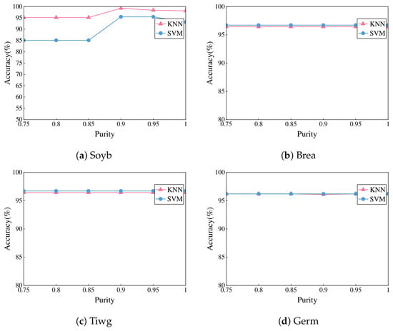
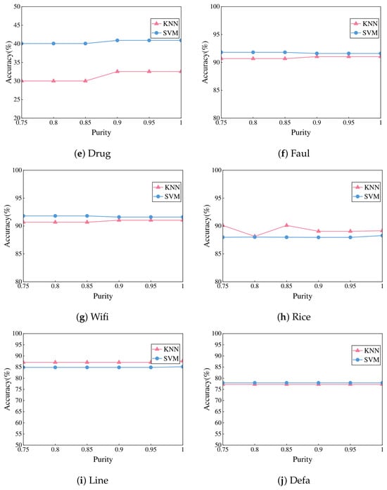
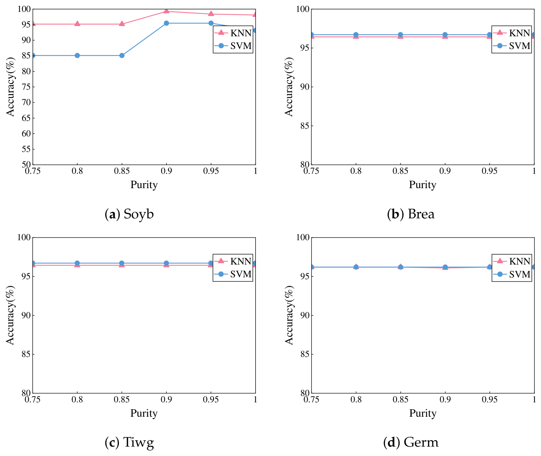
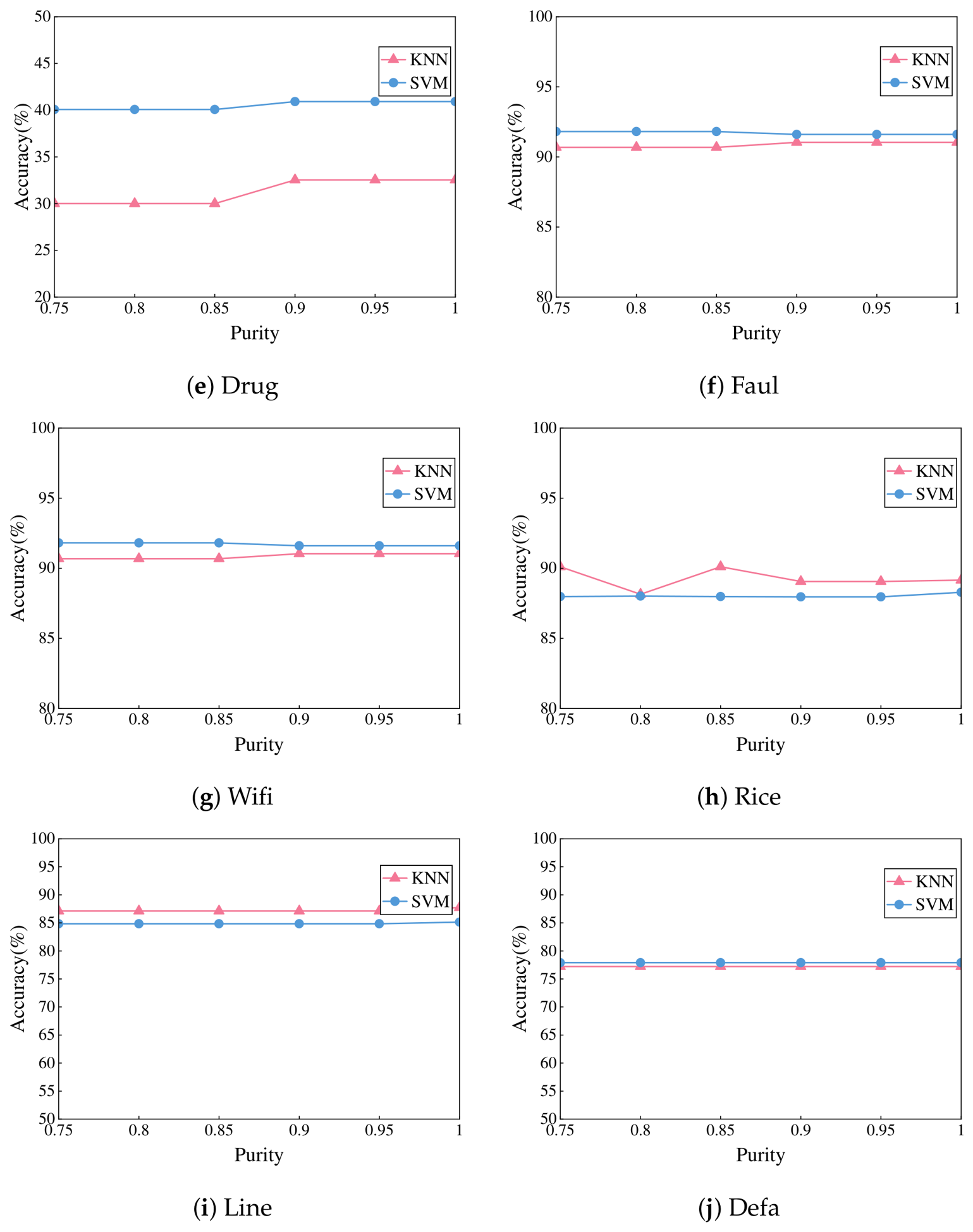
In this subsection, a sensitivity analysis is conducted to examine the effect of the purity threshold $\delta$ on the classification performance of the proposed method. Figure 9 presents the results of the sensitivity analysis. The purity threshold $\delta$ determines whether the fuzzy interval-valued granular ball continues to split. When $\delta$ is 0.90 or higher, the classification performance becomes stable.

Figure 9. Sensitivity analysis.

5.6. Comparison of the Number of Selected Attributes

In this subsection, we compared the number of selected attributes obtained by different algorithms to evaluate their attribute selection capability and the compactness of the reducts. Table 8 presents the number of selected attributes for all algorithms. These results indicate that FRFIGB can obtain more compact reducts for several datasets, thereby demonstrating its strong attribute selection capability.

Table 8. Comparison of the number of selected attributes.

No.	Abbr.	ARIE	ARCE	ARRE	FSPA	FH-IU-AR	CH-HSD-AR	FRFIGB
1	Soyb	10	8	20	8	18	9	9
2	Brea	9	6	9	6	9	9	9
3	Tiwg	22	22	22	22	23	22	22
4	Germ	20	10	11	9	15	12	7
5	Drug	12	12	12	12	12	12	6
6	Faul	16	13	16	13	22	17	3
7	Wifi	7	7	7	7	7	7	5
8	Rice	7	7	7	7	7	7	3
9	Line	17	17	17	17	17	17	17
10	Defa	23	23	23	23	23	23	23

6. Conclusions

Existing attribute reduction algorithms for an $INDS$ typically suffer from high time complexity in both tolerance class construction and the reduction process. To address this issue, this paper proposes TFIGB, an algorithm for adaptively constructing tolerance classes via fuzzy interval-valued granular balls. Based on TFIGB, FRFIGB is developed for attribute reduction and is accelerated by removing objects in the positive region. Experimental results demonstrate that FRFIGB improves the efficiency of attribute reduction while maintaining classification accuracy. The proposed method is mainly designed for attribute reduction in interval-valued decision systems and is applicable to data analysis scenarios where attribute values involve uncertainty, interval descriptions, or measurement errors.

However, this work generates fuzzy interval-valued granular balls with a single granularity. Future work may investigate the generation of fuzzy interval-valued granular balls from a multi-granularity perspective.

References

- Pawlak, Z. Rough sets. Int. J. Comput. Inf. Sci. 1982, 11, 341–356. [Google Scholar] [CrossRef] [Scilit]
- Zhu, Z.; Dai, J. Pairwise Joint Symmetric Uncertainty Based on Macro-neighborhood Entropy for Heterogeneous Feature Selection. Pattern Recognit. 2026, 175, 113051. [Google Scholar] [CrossRef] [Scilit]
- Zhang, X.; Shen, X.; Zhao, W. A novel approach to antinoise multi-granularity classification through graph-based feature selection. Inf. Sci. 2025, 721, 122632. [Google Scholar] [CrossRef] [Scilit]
- Miao, D.Q.; Zhao, Y.; Yao, Y.Y.; Li, H.; Xu, F.F. Relative reducts in consistent and inconsistent decision tables of the Pawlak rough set model. Inf. Sci. 2009, 179, 4140–4150. [Google Scholar] [CrossRef] [Scilit]
- Dai, J.; Huang, W.; Wang, W.; Zhang, C. Semi-supervised attribute reduction based on label distribution and label irrelevance. Inf. Fusion 2023, 100, 101951. [Google Scholar] [CrossRef] [Scilit]
- Yang, J.; Qin, X.; Wang, G.; Zhang, Q.; Li, S.; Wu, D. Attribute reduction for hierarchical classification based on improved fuzzy rough set. Inf. Sci. 2024, 677, 120900. [Google Scholar] [CrossRef] [Scilit]
- Yuan, K.; Miao, D.; Ding, W.; Pedrycz, W.; Yao, Y. Robust Semi-supervised Feature Selection with Multi-granularity Zentropy Modeling. IEEE Trans. Pattern Anal. Mach. Intell. 2025, 48, 4587–4604. [Google Scholar] [CrossRef] [Scilit]
- Dai, J.; Liu, Y.; Chen, J.; Liu, X. Fast feature selection for interval-valued data through kernel density estimation entropy. Int. J. Mach. Learn. Cybern. 2020, 11, 2607–2624. [Google Scholar] [CrossRef] [Scilit]
- Ali, G.; Afzal, M.; Asif, M.; Shazad, A. Attribute reduction approaches under interval-valued q-rung orthopair fuzzy soft framework. Appl. Intell. 2022, 52, 8975–9000. [Google Scholar] [CrossRef] [Scilit]
- Gong, Z.; Sun, B.; Chen, D. Rough set theory for the interval-valued fuzzy information systems. Inf. Sci. 2008, 178, 1968–1985. [Google Scholar] [CrossRef] [Scilit]
- Xu, F.; Lei, J. Approaches to Approximate Reduction with Interval-Valued Multi-Decision Tables in Big Data. J. Softw. 2014, 25, 2119–2135. (In Chinese) [Google Scholar] [CrossRef]
- Dai, J.H.; Hu, H.; Zheng, G.J.; Hu, Q.H.; Han, H.F.; Shi, H. Attribute reduction in interval-valued information systems based on information entropies. Front. Inf. Technol. Electron. Eng. 2016, 17, 919–928. [Google Scholar] [CrossRef] [Scilit]
- Xie, N.; Liu, M.; Li, Z.; Zhang, G. New measures of uncertainty for an interval-valued information system. Inf. Sci. 2019, 470, 156–174. [Google Scholar] [CrossRef] [Scilit]
- Zhang, X.; Jiang, Z.; Xu, W. Feature selection using a weighted method in interval-valued decision information systems. Appl. Intell. 2023, 53, 9858–9877. [Google Scholar] [CrossRef] [Scilit]
- Liu, X.; Dai, J.; Chen, J.; Zhang, C. A fuzzy α-similarity relation-based attribute reduction approach in incomplete interval-valued information systems. Appl. Soft Comput. 2021, 109, 107593. [Google Scholar] [CrossRef] [Scilit]
- Dai, J.; Wang, Z.; Huang, W. Interval-valued fuzzy discernibility pair approach for attribute reduction in incomplete interval-valued information systems. Inf. Sci. 2023, 642, 119215. [Google Scholar] [CrossRef] [Scilit]
- Xu, W.; Cai, K.; Wang, D.D. A novel information fusion method using improved entropy measure in multi-source incomplete interval-valued datasets. Int. J. Approx. Reason. 2024, 164, 109081. [Google Scholar] [CrossRef] [Scilit]
- Xu, W.; Tian, Z. Feature selection and information fusion based on preference ranking organization method in interval-valued multi-source decision-making information systems. Inf. Sci. 2025, 700, 121860. [Google Scholar] [CrossRef] [Scilit]
- Zhang, X.; Shen, X. Graph-driven feature selection via granular-rectangular neighborhood rough sets for interval-valued data sets. Appl. Soft Comput. 2025, 170, 112716. [Google Scholar] [CrossRef] [Scilit]
- Xia, S.; Liu, Y.; Ding, X.; Wang, G.; Yu, H.; Luo, Y. Granular ball computing classifiers for efficient, scalable and robust learning. Inf. Sci. 2019, 483, 136–152. [Google Scholar] [CrossRef] [Scilit]
- Song, M.; Chen, J.; Song, J.; Xu, T.; Fan, Y. Forward greedy searching to κ-reduct based on granular ball. Symmetry 2023, 15, 996. [Google Scholar] [CrossRef] [Scilit]
- Sun, L.; Liang, H.; Ding, W.; Xu, J. Granular ball fuzzy neighborhood rough sets-based feature selection via multiobjective mayfly optimization. IEEE Trans. Fuzzy Syst. 2024, 32, 6112–6124. [Google Scholar] [CrossRef] [Scilit]
- Deng, S.; Zheng, T.; Lai, L. Efficient and rapid attribute reduction based on local t-spherical fuzzy granular ball neighborhood rough sets. Appl. Soft Comput. 2025, 186, 114091. [Google Scholar] [CrossRef] [Scilit]
- Xia, S.; Zhang, H.; Li, W.; Wang, G.; Giem, E.; Chen, Z. GBNRS: A novel rough set algorithm for fast adaptive attribute reduction in classification. IEEE Trans. Knowl. Data Eng. 2020, 34, 1231–1242. [Google Scholar] [CrossRef] [Scilit]
- Chen, Y.; Wang, P.; Yang, X.; Mi, J.; Liu, D. Granular ball guided selector for attribute reduction. Knowl.-Based Syst. 2021, 229, 107326. [Google Scholar] [CrossRef] [Scilit]
- Xia, S.; Dai, X.; Wang, G.; Gao, X.; Giem, E. An efficient and adaptive granular-ball generation method in classification problem. IEEE Trans. Neural Netw. Learn. Syst. 2022, 35, 5319–5331. [Google Scholar] [CrossRef] [Scilit]
- Peng, X.; Wang, P.; Xia, S.; Wang, C.; Chen, W. VPGB: A granular-ball based model for attribute reduction and classification with label noise. Inf. Sci. 2022, 611, 504–521. [Google Scholar] [CrossRef] [Scilit]
- Ji, X.; Peng, J.; Zhao, P.; Yao, S. Extended rough sets model based on fuzzy granular ball and its attribute reduction. Inf. Sci. 2023, 640, 119071. [Google Scholar] [CrossRef] [Scilit]
- Xia, S.; Wang, C.; Wang, G.; Gao, X.; Ding, W.; Yu, J.; Zhai, Y.; Chen, Z. GBRS: A unified granular-ball learning model of pawlak rough set and neighborhood rough set. IEEE Trans. Neural Netw. Learn. Syst. 2023, 36, 1719–1733. [Google Scholar] [CrossRef] [Scilit]
- Chen, Y.; Huang, Z.; Li, J. Fuzzy neighborhood based variable-precision granular-ball rough sets with applications to feature selection. Fuzzy Sets Syst. 2025, 512, 109382. [Google Scholar] [CrossRef] [Scilit]
- Qian, W.; Xu, F.; Huang, J.; Qian, J. A novel granular ball computing-based fuzzy rough set for feature selection in label distribution learning. Knowl.-Based Syst. 2023, 278, 110898. [Google Scholar] [CrossRef] [Scilit]
- Qian, W.; Li, Y.; Ye, Q.; Xia, S.; Huang, J.; Ding, W. Confidence-Induced Granular Partial Label Feature Selection via Dependency and Similarity. IEEE Trans. Knowl. Data Eng. 2024, 36, 5797–5810. [Google Scholar] [CrossRef] [Scilit]
- Xie, Q.; Zhang, Q.; Xia, S.; Zhao, F.; Wu, C.; Wang, G.; Ding, W. GBG++: A fast and stable granular ball generation method for classification. IEEE Trans. Emerg. Top. Comput. Intell. 2024, 8, 2022–2036. [Google Scholar] [CrossRef] [Scilit]
- Gao, C.; Tan, X.; Zhou, J.; Ding, W.; Pedrycz, W. Fuzzy granule density-based outlier detection with multi-scale granular balls. IEEE Trans. Knowl. Data Eng. 2025, 37, 1182–1197. [Google Scholar] [CrossRef] [Scilit]
- Wang, R.; Wan, J.; Li, X.; Tan, S. Fast and robust outlier detection: A granular-ball center isolation and region consistency approach. Pattern Recognit. 2026, 176, 113212. [Google Scholar] [CrossRef] [Scilit]
- Miao, D.; Zhang, N.; Yue, X. Knowledge reduction in interval-valued information systems. In Proceedings of the 2009 8th IEEE International Conference on Cognitive Informatics, Hong Kong, China, 15–17 June 2009; pp. 320–327. [Google Scholar] [CrossRef] [Scilit]
- Yang, L.; Qin, K.; Sang, B.; Xu, W. Dynamic fuzzy neighborhood rough set approach for interval-valued information systems with fuzzy decision. Appl. Soft Comput. 2021, 111, 107679. [Google Scholar] [CrossRef] [Scilit]
- Levandowsky, M.; Winter, D. Distance between sets. Nature 1971, 234, 34–35. [Google Scholar] [CrossRef] [Scilit]
- De Carvalho, F.d.A. Fuzzy c-means clustering methods for symbolic interval data. Pattern Recognit. Lett. 2007, 28, 423–437. [Google Scholar] [CrossRef] [Scilit]
- Qian, Y.; Liang, J.; Pedrycz, W.; Dang, C. Positive approximation: An accelerator for attribute reduction in rough set theory. Artif. Intell. 2010, 174, 597–618. [Google Scholar] [CrossRef] [Scilit]
- Zhang, X.; Mei, C.; Chen, D.; Li, J. Multi-confidence rule acquisition and confidence-preserved attribute reduction in interval-valued decision systems. Int. J. Approx. Reason. 2014, 55, 1787–1804. [Google Scholar] [CrossRef] [Scilit]
- Liu, X.; Chen, B. Attribute reductions based on δ-fusion condition entropy and harmonic similarity degree in interval-valued decision systems. J. Intell. Fuzzy Syst. 2024, 46, 4453–4466. [Google Scholar] [CrossRef] [Scilit]
Disclaimer/Publisher’s Note: The statements, opinions and data contained in all publications are solely those of the individual author(s) and contributor(s) and not of MDPI and/or the editor(s). MDPI and/or the editor(s) disclaim responsibility for any injury to people or property resulting from any ideas, methods, instructions or products referred to in the content. |
© 2026 by the authors. Licensee MDPI, Basel, Switzerland. This article is an open access article distributed under the terms and conditions of the Creative Commons Attribution (CC BY) license.