


Abstract
This article introduces novel methodologies, coordinate systems, and procedures in computational geometry that further develop a Euclidean-based relationalistic framework. The objective is to describe tools using object-oriented relational elements with symmetry, anchored to a fixed point in a relational model, that generate structured point sets serving as blueprints for geometric figures and physical structures representing their source objects. Geometric operations and transformations construct ratio figures and ordered proportional structures. Using discrete -Euclidean geometry, two relational coordinate systems are introduced—polar-vertex coordinates and radial coordinates—both formed through discrete geometric operations. A relational unit circle of fixed magnitude is defined by a 4::1 proportional equivalence between radius and angular ratios, independent of real-number or arc-length geometry. Euclid’s theory of proportion is extended from static abstract magnitudes to symmetry-driven geometric construction, and a square-pyramid geometric blueprint is produced from an Earth ratio figure with accurate dimensional magnitudes. The findings reveal a novel commensurability between the radius of a circle and the side length of a square using a shared fixed point coupled via a 3:4:5 Pythagorean-triple triangle, introducing the concept of ordered proportions.
1. Introduction
The first applications of relationalism within the field of physics are typically attributed to Leibniz in the eighteenth century [1,2,3,4]. Since then, the theory of relationalism has often been treated as a conceptual framework, with exploratory applications in physics having several limitations, including the inability to model motion [5]. Deviating from modern approaches that integrate relational concepts with dynamical approaches and relativistic physics, a novel approach to ‘rishta’ relationalism (RtR) uses discrete mathematics and primitive geometry to model discrete subsystem states [6,7]. The RtR framework is independent of the laws of physics since a temporal node, anchored within a system, does not include any quantifiable duration of time; i.e, it has a zero-dimensional point of time. Although time evolves differently in RtR and different approaches are used to model time, the proposed duration is consistent with Barbour’s notion that time is not fundamental to a system [8].
RtR develops a framework that separates space and time, expanding on descriptive geometry using -Euclidean geometry with indeterminate spatial and temporal points that use observable boundary conditions [7]. The framework uses finite, discrete, natural number magnitudes for construction rather than real-valued geometry, meaning that magnitudes are built from relational geometric ratio units of finite length, which can be interpreted through Euclidean principles and dimensional analysis. The approach aligns in part with Einstein’s standard view of special relativity [9], where descriptions of rods and clocks are fixed by geometric notations. However, relativity transitioned to dynamical theories aligning with symmetries of Minkowski geometry, which Einstein referred to as a ‘sin’ [9,10]. In RtR, the symmetry of primitive Euclidean geometry is non-dynamic and grounded in ordered set theory for labeling elements. In this respect, it aligns in part with Einstein’s original standard view; however, it arises from measurement-bound relations in which time and space remain independent.
An object-oriented centralized point (centroid) is used as a fixed point for symmetry-based modeling, which includes linear and rotational transformation; yet, the approach lacks a formal description [6]. In addition, a centroidal point is modeled without motion or forces [6]. Contemporary relativistic formalisms provide dynamical analyses that assign approximate extrinsic dimensional measures to absolute and primitive relational geometric Euclidean elements that exist between points.
Static spatial relational subsystems are intrinsic (indeterminate), constrained by quantities that can be measured from observations [7]. Geometric magnitudes are information that is both captured and used to model objects and complex relationships in a dynamical system [6,11]. Motion is represented discretely through paired length–time [L · T] elements [11], capturing cumulative displacement analogously to absement, while remaining fully compatible with dimensional analysis and computational modeling [6].
In Rt modeling, object-oriented zero-dimensional points represent the spatial centroids of objects, and a relational configuration at an anchored temporal point encodes all relational magnitudes and angles between these centroids [7]. Partitioning and scale-aware operations preserve angular structure and the recoverable total measure, ensuring that the absolute relational geometry remains intact [6,7,11]. The absolute magnitude of the whole can be recalculated from the scaling and partitioning operations, and in application the whole is reconstructed by recombining the parts. Points are object-oriented relational markers, which preserve the geometric configuration of the intrinsic relational state of the system, with each configuration representing a unique relational subsystem state at a frozen temporal point [7].
Modeling a single object within a broader relational model context, with multiple objects and complex relationships, is yet to be described. One challenge lies in active, discrete construction of geometric figures using transformations and a fixed point within a relational model while incorporating object-oriented ratios, proportional relationships, symmetry groups, group order, geometric transformations, and so forth.
Euclid’s Elements compiles and formalizes geometry into a systematic treatment of points, lines, and planes using space, magnitudes, and proportions [12]. Book V formalizes ratios independent of number, Book VII links ratios to discrete quantities, and Book X distinguishes commensurable from incommensurable magnitudes geometrically. Descartes and Fermat later introduced coordinate geometry, embedding algebra into constructions and enabling systematic representation of curves, forming the basis of modern computational geometry. RtR extends these ideas by integrating geometry with numbers and relational term statements to represent order and symmetry in Euclidean-based object-oriented relational magnitudes [6].
Modern geometric modeling is largely based on analytic and Riemannian frameworks, where space is treated as a continuous manifold endowed with a metric structure that permits infinite divisibility [13], and where metric and differential geometry provide the primary tools for sub-Riemannian geometries.
Riemannian geometry generalizes Euclidean space to smooth real-valued manifolds [13,14], and RtR modeling defines relational lengths that can be physically realized along a flat or curved surface. This means Riemannian geometry provides the mathematical description and prediction of those lengths on curved surfaces [13,14]. Therefore, Riemannian geometric tools can aid in interpreting physical realizations of -Euclidean RtR models when embedded on curved surfaces.
Unlike modern geometric models that rely on predetermined coordinate systems for abstract three-dimensional space, rishta relationalism generates positions relationally from a fixed point [6], avoiding any imposed axes or continuous fields. In RtR, relational space and time are constructed from primitive relational elements rather than being embedded in a continuous manifold, allowing symmetry-driven constructions that cannot be fully represented in Riemannian frameworks.
Primitive geometric elements, such as a relational length required for symmetric -Euclidean modeling, are considered intrinsic, indeterminate elements [7]. This approach aligns with a proposal that primitive geometric concepts, such as length, cannot be derived from dynamics [10] and, therefore, must be assumed a priori. Recent work on the RtR mathematical structure supports this argument by employing observer-based signal operators within a dynamical system to characterize indeterminate geometric elements [7], and previous works have also described that an observer can use determinants and relativistic frameworks to measure primitives, providing significant approximations of absolute dimensional quantities [11].
Descriptive geometry rigorously links three-dimensional objects to two-dimensional representations via projections. In this context, computer-aided design (CAD) workflows, while remaining relevant, face challenges [15]. The rishta framework extends conventional approaches by modeling natural objects as relational point-and-line configurations, generated through discrete operators that preserve relation, order, proportion, and symmetry [7]. Only through geometric transformations, such as rotation at a fixed point, can relational datasets be layered upon a shared surface (flat or non-flat).
Crystallographic frameworks demonstrate that net and lattice spatial structures can be described relationally and through discrete partitions, without reliance on continuous metrics [16]. The core requirements in crystallography include a defined origin, a coordinate notation system, and a rule for specifying atomic positions that allows for comparison [16], and a unit cell is defined as the geometric description that determines how the entire crystal is built through translational repetition. These concepts serve as inspiration for object-oriented modeling; however, rather than using vectors, rishtars encode the geometric information governing relative arrangement. The resulting set of points supports figure traces used to construct a ratio figure of the object being modeled.
Traditional coordinate systems possess limitations in constructing discrete geometric figures from a fixed point; in particular, spacetime coordinates link space and time with continuous motion and cannot represent static -Euclidean geometry, Riemannian coordinates rely on continuous manifolds, and Cartesian coordinates extend into negative and non-natural number values. These constraints motivate the development of new coordinate systems capable of discrete, relational, fixed-point constructions for natural-valued ratio-based geometric modeling.
Regarding works on the development of rishta relational coordinate notation, many historical approaches have been abandoned in modern algebraic mathematics. In eighteenth-century China, Dai Zhen used the term du to denote a primary division of a whole, and the corresponding primary division of an open linear magnitude was termed fang du [17,18]. For closed circular magnitudes, Dai used the term yuandu, analogous to familiar angular measures, and two historical partitions included 360 · 60 · 60 and 120 · 60 · 60 [19]. Open linear-degree symmetry groups were also used by ancient Greek mathematicians for arithmetical notation, [19] (pp. 41–63). Although these linear-degree systems have been abandoned in modern mathematics, combining both open and closed symmetry groups provides useful relationships for developing natural-valued relational coordinates.
String theory combines quantum mechanics with relativity to model fundamental phenomena as extended objects defined within relativistic spacetime, where open and closed strings emerge from boundary conditions [20]. RtR inherently adopted a conceptually similar string-like perspective [21], but replaces spacetime with a discrete relationalistic mathematical framework that applies to both quantum and classical-scale objects. In this analogy, Dp-, D0-, and D1-branes [22] provide useful comparisons, as RtR uses intrinsic (indeterminate) zero-dimensional points and one-dimensional elements between these points, but the methodology separates space and time [6].
RtR’s geometric framework is described as string-like: its relational elements do not span spacetime and are without mass or momentum, similar in part to a previous concept of gravitational point particles with energy and angular momentum equal to zero [23]. Instead, the framework represents intrinsic and unquantified spatial or temporal extensions between corresponding zero-dimensional nodes [7]. Rather than describing particles and their interactions, relational string-like one-dimensional elements (spatial or temporal) are anchored to points in both a real-world system and a relational model of that system. Whole elements are partitioned into symmetry groups and become ordered parts of a whole, acting as discrete constructive geometric elements for building scaled, object-oriented geometric models [6].
This work presents methodologies and tools for constructing object-oriented geometric figures from a fixed point, introducing polar-vertex and radial coordinate systems built on discrete -Euclidean operations. Applications include relational unit circles, ratio-based partitions, and Earth-ratio constructions, demonstrating how symmetry, ordered proportions, and operator-defined relational units can generate complex geometric object-oriented blueprints independent of continuous space or conventional coordinate systems.
2. Materials and Methods
Object-oriented modeling uses both static structure and dynamic behavior, and when applied to physical or signal-driven systems, can include hybrid frameworks that combine continuous processes with discrete event-based state construction.
Within cosmology, geometric and metric frameworks such as Friedmann–Lemaitre–Robertson–Walker (FLRW) and Baryon Acoustic Oscillations (BAOs) are contextualized using a spacetime framework with continuous dynamic modeling systems: the FLRW metric provides a spacetime geometry for the expanding universe, while BAO offers observationally calibrated length scales within that geometry. Viscous fluid cosmology, for example, models cosmic fluids with continuous state variables such as density, pressure, and viscosity, which evolve according to these spacetime metrics to produce phenomena such as effective negative pressure and accelerated expansion [24,25].
In the methodology used herein, dynamical systems with discrete event-signals are modeled as hybrid frameworks in which discrete, non-simultaneous signals index a single spatial subsystem anchored by a unique zero-dimensional temporal point, giving a set of spatial point locations. Spatial point locations are used to construct angles and one-dimensional elements, forming a geometric data stack. Simultaneously, the event signal triggers an automata-like process that uses these elements to construct physical geometric models of objects within that subsystem. Consequently, the modeled objects are generated independently of the system’s evolution in time, with each object uniquely representing data from relational, instantaneous events indexed within a subsystem.
When designing the automata-like process to model objects unique to a given point in time, several key requirements include the following:
- Origin of choice;
- Geometric operations;
- Geometric transformations;
- Geometric figures, coordinate systems, and point mapping.
2.1. Origin of Choice
Object-oriented geometric figures are constructed from a fixed point defined by the object itself in the relational model: a spatial point element with no internal parts, denoted as Object A · ∅s. Each fixed point is within a relational context.
A hierarchical relational model includes overarching square grid structures, referred to as planar nets or grids. For modeling within a physical space, nets are finite since they are bound, anchored, and oriented using markers and limits of the physical structure that it is constructed upon. Each object’s ·∅s origin within a figure construct carries relational information connected to the broader model. Figure 1 shows a fixed point used to construct hexagon and circle traces, coinciding with a point in the relational net. The net and object-oriented spatial fixed point are geometrically indistinguishable in position, and can be identified only through the expanded object-oriented geometric structure from that fixed point.
Figure 1.
Hexagon and circle traced from a fixed point coincident with a net point. Square net point spacing is defined by (i) an Object B · Rt unit magnitude. Point A · ∅s serves as the fixed point for the constructed figures. (ii) Vertices lie at a fixed circumradius from the fixed point, defined by an object A · Rt unit magnitude.
- Hierarchical Internal Relational Grid Rule
Rule: Points on a parent net or within a centered figure construct may be subdivided into subnets (connecting net points) or subcells (internal figure structure). These structures are marked into top-level squares or rectangles. Each top-level element has geometric magnitudes along its width and height, denoted [Lx] and [Ly], respectively. The physical side dimensions and their corresponding ratio magnitudes are determined as follows.
- Top-level magnitude: Let the sides of a figure (square or rectangle) have commensurable geometric magnitudes Mx and My, where and with a dimension of length along width and height, respectively. A square is defined by equal side magnitudes, whereas a rectangle has sides that are commensurable but of different magnitudes (e.g., a 5 Mx × 1 My rectangle).
- Subcells within top-level magnitude: The top-level figure is subdivided into Sx × Sy subcells, where (e.g., 8 × 8 but also 5 × 1), that partition the top-level magnitude along each axis for both squares and rectangles with a quantifiable dimensional property of length:
- Microcell units within each subcell: Each subcell may be further composed of discrete microcells defined by a kl count. The number of microcells along each axis defines a geometric ratio magnitude equivalent to the corresponding top-level side geometric magnitude:where each microcell k-count ratio magnitude along a subcell axis is equivalent in geometric magnitude to the corresponding top-level side, possessing a length dimension and constrained to positive values.
- Notation: The hierarchical grid can be expressed aswhere each subcell is composed of a k-count ratio magnitude.
- Example 1: 1 magnitude × 1 magnitude square with 8(6) by 8(6) subcell structure
- Top-level side magnitude (square side length): 1 magnitude;
- Subcell grid: 8 × 8 subcells;
- Microcell dimensions: 6 × 6 Rtl units per subcell;
- Total square side in kl units: 8 × 6 = 48 Rtl units;
- If 1 m, then x × y ≈ 235.44 m by 235.44 m.
- Example 2: 5 magnitude × 1 magnitude rectangle with 5(1388) by 1(1388) subcell structure
- Top-level magnitude (rectangle side length): 5 × 1 magnitudes;
- Subcell grid: 5 × 1 subcells;
- Microcell dimensions: 1388 × 1388 Rtl units per subcell;
- Total rectangle in kl units: units;
- If 1 m, then x × y ≈ 9296.13 m by 1859.23 m.
In RtR modeling, grids (nets) and figures are constructed using discrete Rt unit structures. Once point markers of the object-oriented net or figures are physically realized, the straight (flat surface) or geodesic (curved surface) line magnitudes can be measured in any standardized unit system, such as meters.
2.2. Geometric Operations
2.2.1. Primitive Spatial and Rotation Elements
Spatial elements used to construct object-oriented figures require geometric elements to be taken from the object itself, referred to as primitive object-oriented elements [7,11].
A spatial primitive (or derived) element is a whole single and uniform -Euclidean linear magnitude but with no breadth, bounded between two Euclidean points of no parts.
The magnitude’s structure is expressed through set-theoretic organization rather than point-set subdivision, as points have no parts and thus have no magnitude. Geometric magnitudes are of the L-domain (length), e.g., .
A typical example of object-oriented primitives consists of two spatial primitives defined by three points on a spheroid: the centroid, a polar tip, and an equatorial point [6] (Figure 2).
Figure 2.
Perpendicular primitive elements from a spheroid. Polar and equatorial primitive elements with corresponding continuous traced circumferences. Centroidal point denoted as ∅s, used as the fixed point for modeling.
Angular elements used to construct object-oriented figures are derived from the partitioning of a whole rotation element, ↻, into parts of a whole, e.g., ∠ABC.
2.2.2. Partitioning Operation of a Primitive (Whole) Element
A whole spatial Rt unit element can be scaled or partitioned. Partitioning a whole Rt unit creates ordered parts of the whole, forming ratio Rt units lesser of the greater whole magnitude [6].
Using an example of a partitioning operation for a spatial length, the following form is taken:
where represents the application of an operation, denotes the partitioning operation applied to the line segment between the zero-dimensional points and , subscript l denotes length for the operation (note: a denotes angle), is the set of all units obtained from the partitioning process, and N is the cardinality of this set of line elements.
The primary division in a partitioning operation establishes a symmetry group generated by the partitioning process. A formal expression of this hierarchical partitioning is given by
where specifies the number of fundamental symmetry divisions, and the subsequent factors represent ordered radix subdivisions that refine the partition without altering the underlying symmetry group.
Additional radix-based subdivisions refine the part within each sector but do not introduce new symmetry elements; they act only as metric refinements of the partition.
2.2.3. Open and Closed Symmetry Groups
To formalize symmetry subgroups arising from closed or open relational elements that possess dimensional properties, including length and duration, the following are required.
- Closed rotational subgroup, : A cyclic group of order n acting on a full rotation about a fixed point. The ordered and finite group is generated by successive rotations that partition the rotation into n discrete sectors, producing n corresponding vertex positions. By convention, a full rotation is measured as 360°, yielding rotation increments of 360°/n. In comparison, generates six rotations measured as conventional 60° each. To encode finer subdivisions along the rotation axis, additional modular indices can be introduced, formingnested or hierarchical subdivisions while preserving the overall rotational group structure, represented as units (a for angular).
- Open linear extension subgroup : A cyclic group of order n acting on a linear magnitude (inner line extension), generated by successive discrete extension steps that divide the extension into n ordered elements. Finer subdivisions can similarly be encoded using modular indices , formingwhich enables nested or hierarchical partitioning along the extension while preserving the overall linear group structure, represented as units (l for linear).
To clarify, previous introductory works by the author [6,11] used dihedral symmetry groups for the first division, , wherein it is clarified that the dihedral group for a completed figure includes the n rotations of and n reflections, giving the group an order of 2n. Although finite in cardinality, carries no inherent sequential order; ordering is introduced through the combination of with the radial extensions, and radixes encode the numerically ordered cyclic structure and arithmetic closure. Dihedral symmetries, such as rotations and reflections, manifest when these groups are embedded within a geometric figure.
From a partitioning operation, the following definitions establish the foundational elements of Rt units used throughout the article.
- Prime Rt unit: A whole or ratio magnitude, which is measured by the unit alone, and an object-oriented geometric element of a uniform and absolute magnitude of one. A prime ratio Rt unit magnitude results from the chosen partitioning operator on a given whole magnitude within the RtR framework.
- Primary Rt unit: The first element in an ordered set of Rt units (), where indexes the set and N is the total number of Rt units produced by the partitioning function.
- Rt ratio, or k-count, magnitude: The uniform magnitude corresponding to an ordered relational count of k Rt units in the set from a fixed point, representing the cumulative magnitude of one composed of these units.
- Submultiples of an Rt unit (e.g., 0.1k, 0.01k) do not create new prime ratio units but act as metric scales—deci-k and centi-k—produced through the partitioning operation (Equation (2)) to refine order and counting resolution while keeping the prime unit as the magnitude reference.
2.2.4. k-Counts and k-Order
Parts of the whole can be organized as k-counts (Equation (5)) or k-order (Equation (6)), offering complementary utility for RtR modeling and scaling [11].
By convention, linear and conventional angular degrees (°) are defined using a cyclic group of 360 divisions. This framework generalizes to a fixed group order n = 360. In contrast, the introduced methodology is flexible and uses a° to denote the ratio-based symmetry group order count corresponding to the cyclic placement of vertices (symmetry group order), while l° denotes the ratio-based symmetry group order count for a linear cyclic magnitude along an inner straight line with no breadth. These -degree units are distinct from k-counts and k-order, which enumerate the order of the total discrete elements produced by a given partitioning operation, including both symmetry and radix group order within each symmetry element.
2.2.5. Relational Term Statements
Numbers are linked to geometric elements, derived from specific variables, partitioning operations, and so on.
For ease of description in the article, variables and object conditions are typically omitted; however, numbers inherently remain associated with the underlying relational geometric quantities, preserving the relational meaning. In term completion, numbers are only meaningful for actual magnitudes when part of a term statement [6].
An open linear Rt unit term for a () magnitude from a defined whole—typically a length or spatiotemporal dimensional quantity/quantities, respectively—can be described as follows [6,11]:
A unit term for linear magnitude extending beyond one whole element can be described as follows:
where represents a count of a whole length equal to N.
Regarding a closed element—typically a rotational symmetry group that can be paired with a temporal period (sample or frame) [6]—Rt unit term for angular unit fractions of a whole rotation can be described as follows [6]:
where represents a count of a whole rotation or temporal period, where .
Closed relational string-like elements can be structured using symmetry groups and fixed points to construct regular geometric structures such as n-gons, which can include concentric nesting. In general group-theoretic terms, simply considering multiple copies of the same symmetry group (e.g., repetitions of ) does not automatically define a new group unless a valid group operation is defined across the copies. A new group of combined orders for temporal frame periods, such as , arises only when the operation (e.g., component-wise addition modulo each group’s order) is formally established. Aligning a frame period with a single uniform whole duration is part of the description. In the spatial and rotational applications considered in this article, however, we treat repeated rotations or periods as a single or group, with W specifying the total count of repetitions, without constructing a higher-order direct product.
To provide an example for linear spatial metrics, we use Earth as an object. Using the partitioning operation from Equation (2) and extrinsic published measurements (the Earth’s polar radius ∼6356.75 km [26] and Earth equatorial radius ∼6378.14 km [26]), we obtain different primary magnitudes that can be quantified by standard units as:
2.2.6. Geometric Elements and Rounding Measurements
Rounding rules apply to dimensional measurements, as quantified precision is limited by available instruments and computational methods.
Absolute geometric elements used for modeling are not numerically rounded, meaning that any unspecified digit is exact; for example, -counts is not rounded to 26.0 or 26. Thus, -counts denotes an exact ratio magnitude of 30. This requires a methodology that preserves discrete equivalence between ratios and proportions.
Dimensional analysis permits standardized units for construction and comparative interpretation; however, averaging across length dimensions removes the geometric relational unit structure. This occurs because both individual figures and composite relational models contain multiple object-oriented primitive-based units or non-primitive (bijective elements)-based ratio-based units; for example, those used in motion modeling [11].
2.2.7. Proportions and Incommensurable Magnitudes
The application of abstract numbers in geometric modeling fails when magnitudes are incommensurable; thus, numbers are used as a component in identifying geometric elements, rather than in isolation.
For numbering, a multitude refers to how many (a count/order number). In Euclid’s Elements, Book VII [12], definition one describes a unit as “a thing existing as one,” which applies to both whole and ratio Rt units, the latter from a partitioning operation. Book VII, definitions two and three, describe a number as a multitude composed of a unit and a number being part of another number, the former lesser than the greater. In application, for RtR, k represents a number for a given ordered ratio unit, part of the number N, and the lesser of the two. Book VII, definition eleven, describes a prime number as one measured by a unit alone, used to define a prime Rt unit, either a whole or a ratio Rt unit. Book VII, definition thirteen, describes a composite number as one that is measured by some number; e.g., . However, composites in number theory describe abstract concepts, so the term ratio magnitude is preferred over composite magnitude.
In Elements, Book V, Euclid’s ratio is introduced to compare magnitudes. In application, the Rt ratio unit is introduced to construct magnitudes, while remaining usable for their comparison. Consistent with the order of Rt units, Euclid’s definition five (Book V) describes the order of the ratios, consistent with 1 Rt coming before 2 Rt, for example. In a linear extension, 2 Rt is twice as long as 1 Rt, yet is constructed in geometric form as a uniform Rt unit ratio magnitude of one line segment between two points.
Unlike Euclid, who maintains a strict separation between continuous magnitudes and numbers as multitudes of units, RtR allows a magnitude to remain continuous while simultaneously being describable as an ordered multitude of an Rt unit count (or order) of natural numbers, providing a ratio magnitude.
In Book X, Euclid distinguishes commensurable and incommensurable magnitudes. A magnitude composed of the same Rt ratio units is incommensurable with magnitudes constructed from any distinct Rt unit(s).
It is possible for two ratio count magnitudes to be equal in length while composed of different units [6]. For example,
Here, ratio magnitudes are both of equal length and incommensurable, which requires them to be derived from the same primitive whole element.
2.3. Geometric Transformations
Object-oriented figures are generated from fixed points through extensions, rotations, and translations. All transformations proceed in discrete steps, consistent with -Euclidean geometry.
- Linear Planar Extensions;
- Translocations;
- Rotation.
2.3.1. Linear Planar Extensions
Open linear extensions for object-oriented construction from a fixed point within a plane use object-derived units. Extensions along perpendicular or oblique axes, such as the z-axis, may be commensurable or incommensurable with planar magnitudes, depending on the chosen primitive element (e.g., polar or equatorial radius of the same object), different objects, relational structure, or partitioning function. Multiple figures can share the same fixed point, producing structures such as concentric n-gons or double pyramids.
2.3.2. Axial Translocations
A figure translocation is defined as the movement of a point, figure, or object-unit cell from one plane to another along an axis. In the case of axial translocations, the fixed point and its associated figure are translated along a principal axis (e.g., the z-axis) while preserving the rotational symmetry within each plane.
Translocations may be fixed, in which the figure maintains a constant orientation relative to the axis, or non-fixed, in which the figure undergoes change, such as simultaneous rotation, extensions, and translation, producing layered or screw-like arrangements such as discrete helical spirals.
The axial positions are expressed using units, ensuring that the relational symmetry and structural proportions are maintained throughout the translocation. Translocation magnitudes can be commensurable or incommensurable with other orthogonal planar magnitudes in the object-oriented figure, depending on the underlying Rt units and object-specific criteria used in the construct.
These combined operations maintain the systematic growth of object-oriented figures from fixed points, supporting the construction of discrete three-dimensional spiral structures, for example.
2.3.3. Rotation
The closed rotational operator acts on geometric inputs in discrete steps, each indexed by an ordered natural number , representing a selected part of a total partition of a full rotation, such that the fractional rotation is given by . The parameter denotes the number of completed whole rotations. Accordingly, the magnitude of a rotational application is expressed as
where can be either count or order.
The partitioning operation (Equation (2)) defines the total number of parts , thereby setting the angular resolution of the rotation. This formulation permits rotational operations to be applied iteratively, with controlled granularity, while maintaining discrete, defined magnitudes.
A figure with rotation symmetry has three vertices and sectors around a fixed point, such that a rotation by one-third of a full turn maps each vertex onto the next, giving an order of three. Within the RtR framework, the same rotation can be represented as a sequence of countable, discrete angular divisions, preserving the three sectors and vertices while capturing the rotation at finer levels defined by the underlying radix-based partitioning operation. Each step is discrete, representing a fundamental departure from classical continuous symmetry frameworks, where rotation symmetries may have infinite order.
Application of the modern convention of a 360° full rotation allows the angular measure to be expressed consistently for contemporary comparisons.
Rotation is defined about a central fixed point on a given plane, which is the object-oriented centroidal origin (∅s). This includes both the parent plane and its corresponding extension into the z-axis for any associated child-plane(s) figures. Rotation can include not only a given unit radial distance (Figure 3a), but also a relational object unit cell, or figure construct (Figure 3b).
Figure 3.
Line segment and triangle unit cell rotation. (a) Equilateral triangle trace (blue) from C3 rotation around fixed point using and subsequent rotation with . (b) Higher-level operation using complex hexagon trace (red) from C2 rotation of equilateral triangle ratio unit cell. Black diamond = start/stop point. Black box = first subsequent vertex point from start (indicates rotation direction). T terminus of radial line = vertex point from given partition step. Vertices from the first-order rotation are shown as an intersection (b). ccw = counterclockwise.
Order-related points support the definition of finer point coordinates that lie between symmetry points in a given geometric figure trace (e.g., circle trace or regular polygon trace, respectively). Points along a trace are defined through radix group actions and are therefore referred to as rotationally ordered points.
2.4. Geometric Figures, Coordinates, and Point Mapping
2.4.1. Figures
Fixed-point figures in physical form can represent zero-dimensional point locations (e.g., the tip of an obelisk), one-dimensional line segments (e.g., the distance between two point markers), two-dimensional configurations (e.g., markers arranged in a circular formation defining polygonal vertices), or three-dimensional structures (e.g., a pyramid).
These figures can be classified according to the origin of the relational units (Rt units) used to generate the point sets used to trace a figure. This distinction clarifies whether a figure is constructed from the internal geometry of one or more objects, from relations between separate objects, or from a combination of both.
- 1.
- Intrinsic figuresFigures constructed exclusively from Rt units derived from object-defined geometries.
- Mono-intrinsic figures: Figures built using Rt units obtained from a single object. Rt ratio unit magnitudes can be either commensurable or incommensurable, depending upon what plane the primitive element is defined in. An example would be using Earth’s polar and/or equatorial radii to construct the figure.
- Multi-intrinsic figures: Figures built from Rt units obtained from more than one object. An example is a composite geometric planar figure giving an egg shape, representing a planetary body together with its orbiting moon(s).
- 2.
- Extrinsic relational figuresFigures constructed using Rt units defined purely through relations between distinct objects, such as the separation between Earth and the Sun. These constructions produce layered system-level geometries and may also include both scaled primitive elements, as well as commensurable and incommensurable magnitudes.
- 3.
- Intrinsic–extrinsic composite figuresFigures constructed using both Rt units from multiple objects and extrinsic relational measures between those objects. These figures encode the internal geometries of individual bodies together with the geometric relations defined by their separations, forming hierarchical structures that may include both commensurable and incommensurable magnitudes.
Within the overarching relational model, a figure can be multi-hierarchical.
A primary fixed point can be defined to anchor the construction of a multi-intrinsic figure within the broader relational model, including a coincident point with a parent net (Figure 2). The approach can also generate concentric n-gon vertex markers using different object-oriented units.
Secondary fixed points may then be established at locations determined relative to the primary fixed point using various geometric constructs, including Pythagorean triple triangles or other vertices, such as one from a primary figure.
A primary figure can also be a geometric blueprint for constructing physical secondary figures. This hierarchical arrangement provides a structured foundation for constructing and arranging multi-intrinsic figures (Figure 4). The method enables scalable modeling of complex multi-object systems while preserving both local and global relational symmetries.
Figure 4.
Multi-intrinsic Earth/Moon circle trace figures with primary and secondary fixed points. Primary fixed point for Earth anchored to parent relational net, secondary fixed point for the Moon anchored to primary figure vertex. Black and grey radii magnitudes are incommensurable, each unit is object-specific, where . r = radius.
2.4.2. Polar-Vertex Coordinate System
Let a figure be defined with respect to a fixed point, with rotational symmetry described by the cyclic group , such that the group action determines the ordered set of vertex directions from a relationally defined anchored axis. Radial distances from the fixed point to each vertex are specified using relational length units , establishing the metric ratio of the construction without reference to angular measurement.
Two levels of rotational ordering are distinguished in the polar-vertex coordinate system.
- Rotation symmetry group order: Denoted , this symmetry defines the underlying cyclic structure of vertex placements about the fixed point. It is independent of the discretization of traces between vertices.
- Rotation symmetry-trace (radix) group order: Denoted , this represents the discrete partitioning of traces connecting vertices, expressed in ratio magnitudes relative to the parent rotational symmetry. These subdivisions refine the internal structure without introducing additional symmetry elements beyond the primary .
After completing a full period, the resulting configuration is considered modulo rotation symmetry , producing a final n-gon structure.
- 1.
- Vertex (V) Coordinate: A discrete point defined by the combination of a radial unit and an element within the rotational symmetry group (Equation (2)) on a defined plane.
- Radius (r): A primary or ratio magnitude from an object-oriented unit specifying the straight distance from the fixed point to a given vertex.
- Rotation: A composition of discrete rotational element(s) with ratio magnitude defined as . Equivalently, θ may be expressed in conventional measurement units as 360°, separate from the method used to construct the vertices (unless specified in a 360-gon partitioning operation). The cumulative effect of these rotational elements results in
- 2.
- Radix Coordinate: A discrete point defined by a radix group and numerical order (or count) partitioning the trace between two vertex coordinates. The radix point coordinate is a tuple.A trace between two vertices can follow multiple paths, such as a spiral, circle, or regular polygon. The latter two are addressed here.
- A posteriori (alpha) vertex coordinate []: A vertex whose position has been instantiated within the coordinate system and figure.
- Radix coordinate: The discrete and ordered position between two vertices within the figure.
- A priori (beta) vertex coordinate ||: A vertex whose position is determined by the figure and cyclic group rules before actual construction or anchoring.
The partitioning of a circle’s arc/chord and a regular polygon’s edge maintains the discrete k-count for an angular partitioning of a rotation.- A circular radix coordinate, denoted by is given by:
- A straight edge (connecting two vertices) defines a radix coordinate, denoted by , where :where may (e.g., regular polygon) or may not (e.g., spiral) equal .
Using k-order notation is both visually and mathematically more convenient for the an Rt polar coordinate system, providing additional functionality for different figure types (e.g., circle vs. polygon).
Square brackets are adopted to denote discrete relational coordinates indexed by natural numbers, whereas round brackets are reserved for continuous real-valued representations used in standard polar coordinates. In this coordinate, vertical brackets denote unrealized vertex state coordinates.
The examples illustrate different demonstrations of how circular and regular polygonal figures can have trace coordinates. Radix coordinates are represented numerically by either angular (arc) or linear (edge) radix subdivisions of or , respectively, without changing the group or total number of rotational subdivisions or magnitude of each -count (Figure 5).
Figure 5.
Relational coordinates for Heptagon and Square. (a) with seven vertices and seven sections, including circle and heptagon traces (red arc and dark blue edge traces). (b) Partial rotation for the heptagon mapped in clockwise (cw) order. Heptagon with . Dashed line representing a single rotation that intersects with a point on the edge or arc trace. (c) Square trace (green) with four vertices and four sections, showing mapped coordinates for a complete counterclockwise rotation. Square with . (d) Equilateral triangle trace (blue) with three vertices and three sections with counterclockwise rotation. Triangle with .
Translocated Fixed-Point Extension
For three-dimensional figures, consider a polar-vertex coordinate system defined in a parent plane with a fixed point serving as the center of a -symmetric construction. If the plane undergoes a translation along an axis orthogonal to the plane (e.g., the z-axis), the fixed point is transported along with the plane, preserving its role as the symmetry center within the local coordinate frame of the translated unit cell point set.
Under such axial translocations, the rotational structure defined by remains invariant within each plane, while the translation introduces a higher-dimensional structure between successive planes. The result is a stacked or layered geometric set of points that can produce a three-dimensional extension of the polar-vertex framework without altering the symmetry order of the original figure.
Multi-planar translocations require an additional axial coordinate for the system, expressed in units, along with corresponding rotational inputs to describe orientations along perpendicular or oblique axes between planes. This necessitates more advanced notation, which is beyond the scope of the article.
2.4.3. Relational Unit Circles and Squares: Uniform Magnitude of One
The discrete relational unit circle represents both angular and radial components for a given rotation.
An angular unit is a part of a whole rotation defined by relational angular units,
where denotes a primary unit, indexes angular units, and n denotes the symmetry group for the whole rotation. N denotes the partitioned whole, or cardinality of the set, while denotes the count of a full rotation, where if , then . For example, . Each unit magnitude can be partitioned into submultiples.
Five types of uniform radius magnitudes are applicable to an Rt unit figure (Box 1).
Box 1. Uniform, open, and straight magnitude types for unit figure constructs
- Primary ratio magnitude (), representing the base unit;
- Submultiple ratio magnitude (), representing a portion of the base unit, e.g., or , with natural number counts defined through the partitioning operation’s · ⟨base-10z⟩ groups (Equation (2));
- Inner ratio magnitude ( but not a whole multiple), representing a physical sum of a primary unit and a submultiple (e.g., units);
- Whole magnitude (), representing one full partitioned line element;
- Greater-than-whole magnitude (), including exact multiples of a whole (e.g., ), as well as magnitudes larger than one whole unit (e.g., ).
The partitioning operation and symmetry group assigned for discrete rotation symmetry and linear extensions (radius) are independent.
2.4.4. Relational Unit Circle: Construction, Proportions, and Coordinates
A relational unit circle does not pre-exist; the circumference is constructed as a continuous arc trace connecting discrete points with a countable infinite cardinality (dependent upon the partitioning operation, Equation (2)). The construction begins from an anchored fixed point and proceeds by utilizing one magnitude of a uniform object-oriented radius.
A circle trace connects discrete points from radial extensions and rotations, constructed as a proportion with equivalence between two relationships, a linear ratio (parts of four times the radius [r]) and an angular (or rotational) ratio (parts of one whole rotation symmetry).
where
A radius is a single uniform magnitude; yet, it can be measured by object-oriented unit(s). A rotation is represented in discrete unit steps. Each ratio part of a whole linear or angular relationship uses natural-value counts (Figure 6).
Figure 6.
Open/Closed relationship in unit circle Trace. Counterclockwise rotation using discrete angular units, where . One uniform radius magnitude measurable in units, where and . Dashed arrows represents direction of ordered addition for each radial line. (a) Point coordinates at front of (blue) trace using intersect at . For comparison, trigonometric sin(θ) is shown, Point (i). Point (ii) is the k-order of related to the circle trace point coordinate. (b) Equivalence of full rotation and linear extension relationships for constructed relational unit circle, a:b::c:d. (c) Linear illustration of k-order of units in relationship with (d) k-order of units in geometric proportion, including unpaired and paired coordinates for circle trace points (i) and (ii).
The parts of a ratio in each linear and angular relationship are used as a coordinate system for incident points in a trace circle front. The trace results in a discrete quadrant rotation during construction (Figure 6b).
When both linear and angular partitioning operations use ⊖ = 360 · 60 · 60, for example, the relationship of a whole Rt unit circle (1 rotation) yields the linear–angular proportion that can be shown in various ways:
2.4.5. Relational Unit Square: Construction and Coordinates
Rt Unit Square Construction
An object-oriented construction of a relational unit square begins with a fixed point. As discussed with a relational unit circle, points trace the edges of a square, much like their use for a continuous circle trace. Construction integrates rotation symmetry, which can include a proportion statement.
Each square side is defined by a uniform object-oriented magnitude (Box 1), forming edges that are commensurable. These edges separate four vertices, creating a two-dimensional unit cell with a figure trace.
An object-oriented square centered on a point with sides equal to is introduced as a primary Rt unit square. The center uses a fixed point as the object origin (Figure 7a). A primary Rt unit square is constructed as an inscribed figure within an irrational quadrilateral using rotation symmetry and an inscribed primary square with a side of (Figure 7a,b). Two full rotations with an extension after each full rotation constructs a square with side magnitudes equal to (Figure 7d).
Figure 7.
Centered/fixed primary and ratio Rt unit square construction. Rotation and spatial symmetry partitioning operations: , respectively. The letter F shown to indicate rotation, orange line represents inscribed square. (a) Radius of before rotation. (b) Irrational quadrilateral (green) constructed with a complete rotation using , with an inscribed prime unit square centered at the object origin. (c) Inner dotted squares with submultiple sides (0.8 and 0.6 ). (d) Two rotations with extension of provide discrete points for continuous tracing a 2 by Rt unit square. (e) Simplified rotation symmetry in the construct.
For coordinates, finer subdivisions between vertices can be measured using modular (radix) indices with —for example, —which aligns with conventions of 90° per quadrant while preserving the underlying structure for rotational symmetry in standard quadrant-based constructions.
For an object-oriented polygon centered on a fixed point, a radial line is defined as the line from the center to the midpoint of an edge, representing the shortest magnitude from the center to the boundary (Figure 7). For example, a unit circle has a radial line equal to , whereas a 2 × 2 unit square has a principal radial line equal to .
A principle radial line is used for establishing a symmetry line for physical modeling. Embedding a figure in a larger physical relational model, the principal radial line marks the symmetry line with a defined reference vertex that is aligned with markers from the physical environment or model itself. Examples include a cardinal direction on the spheroidal object (planar or 3-D), or even a sunrise point for a solstice event.
Harmonizing geometric figures, group theory, and physical relational modeling in a rotational symmetry diagram of an n-gon, the identity element e corresponds to the orientation where the chosen principal radial line points to the reference vertex, representing zero rotation.
2.4.6. Radial Coordinate System
In analogy with Cartesian coordinates, a relational non-Cartesian representation is introduced here as a radial coordinate system. Radials can be structured along four radial lines for a rotational symmetry, with each line measured in discrete object-oriented units. Oblique angles with rotational symmetries () are not included here.
There are two types of radial coordinate systems, as follows:
- Commensurable radial coordinate system: Each radial uses identical Rt units.
- Incommensurable radial coordinate system: Two or more radials sharing the same fixed point use different Rt units. These can be along planar perpendicular axes (e.g., x, y) and/or along an axis perpendicular to the plane (e.g., z).
Notation can include the x, y, and z axes; however, various differences exist. First, two planar perpendicular axes x, y only apply to a rotation symmetry. Second, the Cartesian origin (0, 0) is not consistent in the radial coordinate system. In a radial coordinate system, the fixed-point origin anchors the figure in the larger relational model (). The starting point is defined by a linear-degree coordinate , which specifies the stop/start position on the principal radial line of the planar two-tuple (Figure 8). Lastly, x, y, and z axes are defined with fixed, uniform object-oriented magnitudes, measurable by internal units along each axis (Box 1). Radial lines of unit magnitude (r = 1) measured in units combine under rotation to a total magnitude of 4r, and the use of k-order indexing ensures compatibility with the partitioning scheme while preserving natural-number–valued mappings over the traced coordinates (Figure 8).
Figure 8.
Inscribed 2 by 2 Rt unit square construct. (a) Quadrants are generated by the action on the principal radial line (shown as an inscribed square (orange) trace with two complete rotations). Two-tuple radial coordinates assigned using k-order of discrete vertical (quadrant I) shown along the y-axes, horizontal (quadrant II) shown along the x-axes, vertical (quadrant III) shown along the y-axes, or horizontal (quadrant IV) shown along the x-axes, with radial linear–symmetry extensions beginning at the centroid for each quadrant rotation. (b–e) Rotated for x, y designation. (f) Total radial magnitude, where each position along the line segment is a unique count/order. Black diamond = starting and ending point of the internal coordinate system from the traced square. Black diamond = inscribed unit circle start/stop position in a rotation. Curved arrows represent direction of discrete rotation for quadrant of inscribed square.
The proposed axes notation is , where the primary radial line used as the start of a rotation symmetry of the coordinate is notated as (Figure 8). The designation of r alone, without a subscript, is conventionally referred to as the radius magnitude. Therefore, in a given rotation symmetry , there are radial lines with n vertices and sectors.
Several options exist for standardizing radial coordinate notation. One approach adopted here aligns the notation with and (x, y) pairing order at each step of rotation. Within a symmetry, linear-degree measurements ( units) over the total radial magnitude are expressed as ordered coordinate pairs, similar to (x, y) (Figure 8):
- Quadrant I ()
- –
- Radial: extension from ;
- –
- Rotation: 0° to 90° (conventional measure), or ;
- –
- Radius magnitude in k-order/count: 0 ≤ r ≤ 1;
- –
- Two-tuple radial linear-degree coordinates ( units): from paired with from , denoted , with each input representing a position in the total count.
- Quadrant II ()
- –
- Radial: extension from ;
- –
- Rotation: 90° to 180° (conventional measure), or ;
- –
- Radius magnitude in k-order/count: ;
- –
- Two-tuple radial linear-degree coordinates ( units): from paired with from , denoted , with each input representing a position in the total count.
- Quadrant III ()
- –
- Radial: extension from ;
- –
- Rotation: 180° to 270° (conventional measure), or ;
- –
- Radius magnitude in k-order/count: ;
- –
- Two-tuple radial linear-degree coordinates ( units): from paired with from , denoted , with each input representing a position in the total count.
- Quadrant IV ()
- –
- Radial: extension from ;
- –
- Rotation: 270° to 360° (conventional measure), or ;
- –
- Radius magnitude in k-order/count: ;
- –
- Two-tuple radial linear-degree coordinates ( units): from paired with from , denoted , with each input representing a position in the total count.
An alternative two-tuple coordinate pairs a selected count from the total radial magnitude () (Figure 8f) with a rotational count or measure (e.g., or ).
An Rt unit square has commensurable sides and internal coordinate point spacing derived from a partitioning operation and its submultiples. Theoretically, grid coordinate spacing for physical modeling can be subdivided to Planck-scale resolution.
For a whole Rt unit square, each side equals N-counts of the whole magnitude (), where the whole length is treated as a primitive object-oriented magnitude (e.g., a semi-minor axis) (Figure 9b). Squares may also extend beyond this scale, where (Figure 9a). For example, if constructed using Earth’s polar radius as the primitive length, the square side () equals the magnitude of the polar (rotational) axis, with Earth’s centroid representing .
Figure 9.
Whole Rt unit(s) square trace. (a) Rt unit square with side length of , with inner ratio Rt unit squares in a 4(2) × 4(2) arrangement. (b) Quadrant I: Rt unit square with side lengths using fixed point rotation symmetry, with inner ratio unit squares in a 2 × 2 quadrant arrangement. Point (i) showing coordinates, point (ii) showing coordinates, and point (iii) showing the vertex polar coordinate (purple). .
2.4.7. Relational Circle/Square Traces: Commensurable and Incommensurable Magnitudes
This section presents methods for three planar trace figures (circle circumferences and squares) from connecting discrete points using arcs or lines, constructed from the same fixed point, with variations in the proposed intersection point coordinates.
Rotational measures are defined as , or (). The square construct uses a radial magnitude from a whole unit, partitioned into .
- Whole Rt unit square with inscribed circle trace: An Rt unit circle arc trace in quadrant I uses a linear radius of (Figure 10). An inscribed arc trace line uses 90 a°-counts in a clockwise direction for Quadrant I.Figure 10. Quadrant I of Rt unit square with inscribed circle. Point coordinates in quadrant I using convention for quadrant. .
- Rt unit square with commensurable circle radius magnitude: Using a Pythagorean triple triangle (3:4:5) embedded within the bound unit ratio magnitude square, the procedure generates a ratio circle radius with a commensurable magnitude to the linear-degrees unit, measured side (Figure 11).Figure 11. Quadrant I of arc with radius commensurable to unit square side length. Whole Rt unit square with an inscribed 3:4:5 triple triangle in quadrant I with relationally nested 8(x) by 8(x) and 10(x) by 10(x) squares. Hypotenuse used as the radius , for the traced arc of the circle and has a magnitude commensurable with the sides of the linear Rt unit square(s). Coordinates using either or convention introduced here. .A 3:4:5 coupling triangle is defined as a Pythagorean triple with commensurable side magnitudes, each measured using the same ratio unit:A 3:4:5 triangle is constructed with respect to a prescribed fixed point (origin of choice), located at the intersection of its and sides, where is specified as the k-count or k-order of the ratio unit . This origin serves as the center for generating object-oriented geometric figures that are coupled to the triangle and with commensurable magnitudes using a common unit of measure.Linear magnitudes, such as square sides and circle radii, are commensurable when constructed from the same ratio unit, in accordance with the Natural Commensurability Rule (see Section 3). Derived traces, including circle circumferences or polygon perimeters, are not inherently commensurable. Using the Discrete Circle Postulate, discrete vertices generate circle geometry, while the Proportional Coupling Rule preserves ratios from primitive figures (see Section 3); however, the resulting traced circumference remains incommensurable with the square perimeter despite both figures being built from commensurable units.
- Circle with radius incommensurable to unit square side length. A circle can be geometrically constructed using the vertices of an Rt unit square such that its radius is incommensurable with the unit used for the square’s sides (Figure 12). However, this example illustrates the concept only. Using an irrational radius without an associated scaling system for a secondary unit (unpublished) would be inconsistent with the RtR methodology, which relies on discrete, natural-number–valued magnitudes.Figure 12. Quadrant I of arc with radius incommensurable to Rt unit square side length. Point coordinate in quadrant I using and/or for comparison. Black diamond = start of quadrant, red arc = trace, grey dashes = two lines of symmetry for full square with four quadrants.
3. Foundational Postulates, Operations, and Logic Rules of RtR
The following organized postulates establish the primitive objects, allowable operations, and logical rules that govern the RtR framework for object modeling described in this work.
- 1.
- Structure of time and spatial subsystems: Standard continuous time is treated as a smooth linear continuum with no start or stop (e.g., t ≠ 0). In contrast, relational time is intrinsic, existing outside of spacetime, constructed between anchored discrete zero-dimensional temporal point elements relative to a spatial point. A relational location of a unique spatial point is intrinsic to the point itself and is not defined with respect to any Cartesian coordinate system. Temporal progression measurements are discretely indexed between static subsystem states of spatial points, referred to as absolute point time [7,21].
- (a)
- Zero-temporal points: Zero-temporal points are unanchored zero-dimensional elements of a discrete temporal geometry with no duration.
- (b)
- Temporal nodes: A temporal node, , is an anchored zero-time point at which relational durations begin or terminate and does not serve as an arbitrary reference marker (a temporal point position) [6,7]. Temporal nodes anchor a temporal point in a memory system, indexed using a distinct relational spatial history (or snapshot) of spatial point locations relative to a reference point.
- (c)
- Finite durations: Finite intrinsic durations are constructed as ordered one-dimensional elements between successively anchored temporal nodes. Intrinsic elements are measured by extrinsic tools, such as relativistic frameworks [7].
- (d)
- Absolute point time: There exists a universal and uniform separation of a discrete count of time that passes through every zero-dimensional point anchored within a changing system, each discrete “tick” exists outside of spacetime and independent of Newton’s absolute time that is modeled in three-dimensional space [21].
- (e)
- Omnipresent universe: The universe is treated as having only one temporal instantaneous present. This theoretical present fits well with Aristotle’s concept of the present now, existing outside time [7].
- (f)
- Spatial subsystem: A spatial subsystem is defined as a discrete spatial geometric domain of spatial points in -Euclidean space indexed by a temporal node [7]. Zero-dimensional spatial points exist within this domain in relation to each other, forming the primitive spatial elements (extensions) and angles of the subsystem.
- 2.
- Primitive Spatial and Rotation Geometric Objects: Primitive spatial geometric objects, consisting of zero-dimensional points and one-dimensional line elements with finite-dimensional magnitudes, exist within a given subsystem. Each subsystem is defined at a temporal node anchored at instant y, paired with its set of spatial points to form discrete relational tuples,where i indexes the set of spatial (s) point elements at the temporal point (y). Temporal indexing does not create these objects but, instead, organizes them into a primitive geometric memory stack that encodes the relational order of points, their one-dimensional extensions, and associated angles within each subsystem.
- (a)
- Points: Spatial points have zero-dimensional quantities and no relational location unless defined. Spatial nodes are spatial points anchored to a defined spatial location at a given temporal node y [7], such as the Earth’s centroid at the spring equinox in 2026.
- (b)
- Line segments: An intrinsic, uniform whole straight line is fixed between spatial nodes (extension) or temporal nodes (duration).
- (c)
- Magnitudes: A one-dimensional Euclidean geometric line segment represents one or more dimensional quantities and can be partitioned into a natural number of k-counts/(order-of-ratio) units. Whole elements or parts of a whole are measured by extrinsic tools, such as relativistic frameworks and rulers [7].
- (d)
- Rotation: A whole rotation around a fixed point is a geometric measure of an angle that can be partitioned into a number of -counts/order of ratio units, .
- 3.
- Discrete Circle Postulate: Let a discrete circle be defined as the set of points generated by the discrete rotation of a fixed radial magnitude about a fixed center, such that each point is equidistant from the center. The points are produced in an ordered sequence, and adjacent points may be connected by arc elements to trace the boundary, defining the circumference.
- (a)
- The radius magnitude of a relational discrete circle is uniform, derived from relational units.
- (b)
- Each discrete rotational step defines a vertex. The number of vertices may be chosen according to the desired n-gon using a whole rotation partitioning operation that can generate units, which can generate a cord length to the limits of Planck length.
- (c)
- The discrete circle circumference is a derived continuous trace connecting these equidistant points and lies outside the discrete framework.
- 4.
- Permissible Operations
- (a)
- Partitioning operation: A whole geometric magnitude (rotation, extension, or duration) is partitioned into an ordered set of discrete Rt units, establishing structured subdivisions for subsequent constructions.
- (b)
- Point-fixing operation: The point-fixing operation maps an object-oriented spatial node, , from within a relational subsystem -Euclidean space to a defined origin of choice in the finite modeling grid. The fixed point, represented as , establishes a reference for subsequent constructions or transformations of fixed-point object-oriented figure(s).
- (c)
- Discrete rotation operation: Rotation partitions a whole angular magnitude into ordered -counts via units about a fixed point, specifying angular positions only; placement of elements is separate, and continuous circular tracing is excluded.
- (d)
- Addition of magnitudes: Ratio magnitudes are constructed by sequential, ordered addition of Rt units from a fixed origin; conjunction occurs only at discrete points.
- (e)
- Geometric coupling operation: Applying geometric figure constraints (e.g., 3:4:5 triangles) to link linear and radial magnitudes for coupled figures via shared Rt units to a shared fixed point.
- 5.
- Logical Rules
- (a)
- Natural commensurability rule: All derived measures are constructed as finite combinations of discrete relational unit magnitudes indexed by natural numbers. Commensurability is not assumed a priori, as in real-valued spaces where comparability is inherent, but is established only through explicit construction from relational unit elements of the same set.
- (b)
- Discrete evolution rule: Geometric constructions proceed via discrete steps rather than continuous transformations.
- (c)
- Fixed point rule: Certain points (e.g., origin of choice) serve as reference centers for derived fixed-point object-oriented figure constructions.
- (d)
- Proportional coupling rule: Higher-order figures preserve the proportional ratios established by coupling features from primitive geometric figures such as Pythagorean triple triangles or squares.
- (e)
- Object-oriented independence: Each figure or magnitude is defined relative to shared points and ratio units; figures are not embedded unless explicitly constructed.
4. Example: Earth–Object Square, Circle, and Pyramid
For this example, geometric procedures include partitioning operations for rotation symmetry of , planar and orthogonal (translation) linear extensions . ratio units are defined from the selected object, Earth, using both polar radius (semi-minor; smn) and equatorial radius (semi-major; smj) as pre-partitioned primitive elements. The square base, circle radius, and height of the pyramid are constructed using rishtars partitioned from Earth’s planar axes (Table 1) and geometric transformations.
Table 1.
Earth-oriented derived and primitive whole magnitudes shown in Rt units and standard meter units.
4.1. Commensurable and Earth-Oriented Circle/Square Trace: 3:4:5 Triangle Coupling
Starting from a fixed point, the generated point set forms an object-oriented unit cell based on a 3:4:5 triangle. Using this point set, various geometric constructs were traced, including regular hexagons, complex hexagons, squares, and circles (Figure 13).
Figure 13.
Ratio Unit Cell of Earth. Radial distance of with rotation symmetry, and using a 3:4:5 triple triangle for a commensurable coupled relationship between the side lengths and the circle radius magnitudes. Red = circle trace, blue = square trace, purple = 6-gon trace, black diamond = start/stop of discrete rotation, shaded grey Pythagorean triple triangles represent first and last of six discrete rotations that provide vertices for 5-gon.
After six sequential transformations, each increasing the radial distance by one unit cell dimension per rotation, the radial distance increased cumulatively by a factor of six (Figure 14). The resulting radial distance can be quantified as
Figure 14.
Two-dimensional relational squares with commensurable circle radius. Figure composed of an inner 8(6 ) by 8(6 ) ratio Rt unit squares. Outer 10(6 ) by 10(6 ) ratio Rt unit square with side magnitude equal to the diameter of the inscribed circle, terminal point using coordinate notation in counterclockwise rotation. Principal radial line aligned with physical anchor point, North Pole. Red circumference of circle trace, orange and blue traced sides of squares.
Consequently, the figure is composed of a subcell (microcell) grid, with each side having a top-level magnitude of
This results in the sides of the square microcell with a magnitude of
Perimeter Calculations
The perimeter calculations presented aim to quantify geometric relationships between square perimeter magnitude and derived circular traces using a natural-valued unit commensurable radius magnitude, highlighting the inherent differences between a continuous circle trace and the commensurable magnitudes of the radius and the square sides.
Using modern mathematics and standard units, the calculated circumference (C) of this circle trace is
The circumference (and radius), therefore, corresponds to a 1:43,200 ratio of a circle’s properties using Earth’s polar radius of .
It is noteworthy that, if the interpreted partitioning operation for the diameter of a circle, p. 49 [19] by Ptolemy, is used for a radius,
then the radius of the circle in Figure 15 (147.1470 m) corresponds to an equal yet incommensurable magnitude using two unique Rt ratio units as
Figure 15.
Basic square pyramid using Earth metrics. Inscribed square pyramid object; 3D spatial figure using ratio Rt unit cell with Rt lattice created using 6 axial rotations, 6 linear extensions of ratio Rt unit cell, and 6 vertical translocations using units derived from Earth’s equatorial radius (semi-major axis). The green dotted arc is a visual representation of the equator for reference. . Blue represents the basic square pyramid ratio of Earth.
The calculated perimeter (P) of the great square trace is:
The perimeter of the 8(6) by 8(6) and 10(6) by 10(6) squares, therefore, correspond to a 1:6750 (Figure 15) and 1:5400 ratio of the object’s polar radius, respectively. In turn, the side of the 8(6) also has a 1:27,000 ratio of the object’s polar radius.
These calculations demonstrate that the derived circle circumference and the square perimeter are not commensurable, even though the square’s sides and perimeter share a ratio unit with the circle’s radius. The derived circumference trace predictably differs from the square’s perimeter—in this example, by approximately 1.94%. However, in contrast to a traced continuous circumference, no difference is observed under a 4::1 linear-to-angular relationship in a relational unit circle (Figure 6).
In accordance with the Natural Commensurability Rule, all figures in this framework are constructed from finite combinations of discrete relational unit magnitudes indexed by natural numbers, ensuring that the magnitudes used in constructions are inherently commensurable. The Proportional Coupling Rule further ensures that higher-order figures preserve the proportional ratios established by primitive geometric features.
Under the Discrete Circle Postulate, circle geometry is generated from vertices produced by discrete rotations of a fixed radial magnitude, enabling a derived circumference trace. As a consequence, the radius-to-circumference ratio (1:π, Equation (31)) demonstrates that the continuous circumference is not commensurable or of equal magnitude with the square perimeter (Equation (35)), while the construction of both figures relies exclusively on magnitudes that are commensurable according to the same relational unit set.
4.2. Basic Square Pyramid Using Z-Axial Translation
In this step, six concurrent axial translations expand the point set into three-dimensional space along the z-axis using open linear ratio units. The central fixed and planar set of points was translated vertically from the parent plane in six discrete increments, each spaced by
along the z-axis.
The operations generate a set of points in a three-dimensional lattice that can be used to trace a square pyramid object (Figure 15)—an object that can serve as a blueprint for a physical geometric object.
The described operations provide a height to the basic square pyramid object equal to
The conceptual framework further permits switching between Rt units for planar constructions, whereby the architect can instead use Earth’s equatorial-radius-defined units and axial translations defined by polar-radius units. As a result, two nested square projections and corresponding heights can be obtained. The slightly larger, or great equatorial square is generated using Earth’s equatorial radius as unit magnitudes (perimeter ≈ 944.9088 m), while the height derived from Earth’s polar radius units is correspondingly shorter, ≈147.1470 m.
Three-dimensional space emerges from the perpendicular composition of relational two-dimensional planes, built atop one-dimensional extensions between ontologically real points. The three-dimensional figure presents a volume that can then be utilized further to represent quantities related to the object in the physical model; for example, this could include a mass ratio.
4.3. Ordered Relational Proportions: Circle/Square
The aim of this section is to introduce how natural-valued ratios, proportions, and ordered proportions are developed. A relational (ordered) proportion is a coupling between two otherwise independent geometric-based proportions in which variation in one induces a corresponding variation in the other through shared geometric magnitudes. The antecedent and consequent are not numbers—they are geometric magnitudes.
Unlike modern notation, where an antecedent and consequent typically represent a numeric value, this method aligns with the Euclidean use of geometric magnitudes, as in golden proportions, which can include one or more components.
In the examples presented here, the aim is to demonstrate that each ratio within a given proportion belongs to a different symmetry class: the first designated ratio is governed by the discussed open linear symmetry and the second ratio is governed by the previously proposed rotational symmetry class . However, interoperability is noted. Unlike prior treatments in which ratios are inverted to conform to a divisional form [11], this work defines an internal ratio as a part of a whole element, expressed as 3:12 rather than 12/3.
First-order proportions have a relation between two ratios, e.g.,
A novel geometric link between these two proportions was discovered in the geometric relationship between circle and square traces from the set of points.
A second-order proportion is, therefore, introduced as a relational equivalence between two first-order proportions, denoted as ∴; e.g.,
A consideration for an untested third-order proportion may logically follow a linked coupling, or relation, between two second-ordered proportions.
Higher-order proportions are defined recursively as relations between lower-order proportions. For coupling, a link is required between the geometric figures.
In classical proportions, cross multiplication solves for an unknown assuming that all terms are numeric and of the same type; e.g., . In contrast, this framework uses geometric magnitudes of different symmetry classes (e.g., (linear) spatial vs. rotational), so relational proportions are expressed with :: rather than =. Variation in one proportion propagates geometrically to the linked proportion, preserving commensurable ratios and enabling construction of ratio figures such as circles and squares from object-oriented magnitudes.
Example 1.
Using the object-oriented model of Earth and the concentric square and circle constructs (Figure 14) both use commensurable magnitudes (side and radius) for their tracings. The two figures are coupled through a coupled relationship using the 3:4:5 Pythagorean triple triangle, introduced as . Square and circle proportions (the square arbitrarily shown as the first proportion) are represented as and , respectively, and represents the symmetry class of the partitioning operation in the given ratio of the proportion. A multiplication of the object-oriented figure constructs is represented by x, preserving figure proportions where .
Square proportion (open symmetry group):
Circle proportion (closed symmetry group):
Using the concentric square/circle Earth-oriented figures from above, the magnitude term statements from the figure are expressed in their respective first-order relational proportion statements (Equation (41)). For simplicity, the object-oriented designation in each term is omitted; this highlights that the methodology can use the whole element of any object, as defined. .
Combining modern mathematics with geometric tracings, 2π cancels out from the ratios at the completion of a compass tracing. Shown as first-order proportions, the relationship for the second-order proportion is a .
Example 2.
Using the previous second-order proportion from Example 1 (Equation (41)) with coupled relation and noted rotation symmetry group , let d (Equation (42)) correspond to : (reduced from c:d, :86,400 ). Solve for b (the side of 8(x) by 8(x) square), f (radius of the circle), and (ratio magnitude of circle figure) under this assignment.
Thus, a is determined as the side length of the square, giving a ratio magnitude for the unit square side of
Using a 3:4:5 Pythagorean triple relation for the second-order proportion, the hypotenuse used as a radius for the circle construct is then
preserving the commensurable ratio unit magnitudes throughout the second-order proportion and the construction. The hypotenuse represents antecedent e in the ratio e:f. We now determine the corresponding ratio within the symmetry group for the figure by setting and solving for h.
5. Discussion
This work introduced a framework using discrete -Euclidean methodology for constructing physical ratio-based geometric figures of real-world spherical and spheroidal objects. Object-specific spatial rishtar elements and geometric transformations were used to define a set of points used for tracing figures. In addition, novel coordinate systems and construction procedures were presented, enabling the generation of structured point sets without reliance on real-valued metrics, arc length, or differential geometry.
The article addresses a previously missing step in rishta relational modeling [6,11] by explicitly linking the formation of relational units (rishtars) to their role in constructing object-specific physical models. These models originate from a fixed point embedded within a larger relational framework, allowing objects to be mapped hierarchically using properties consistent with points embedded in a two-dimensional net or grid-like pattern or three-dimensional relational lattices.
5.1. Extension of Euclid’s Theory of Proportion
Euclid’s theory of proportion is extended from static magnitudes to symmetry-driven geometric operations. Proportions in this framework govern object-oriented geometric construction rules rather than purely abstract measurements, allowing classical proportional reasoning to operate within discrete geometries. This extension provides a constructive interpretation of symmetry and proportionality compatible with fixed-point–based systems.
Euclid treats ratio as a comparative relation between magnitudes of the same kind (Book V), the unit as an arithmetic part composing a whole (Book VII), and commensurability as the existence of a common geometric measure (Book X), without assigning ratios a constructive role [12]. In contrast, the RtR framework redefines ratios as ordered, dimensionally quantifiable units that discretely generate magnitudes from a fixed origin and function simultaneously as generative and comparative elements using rotation and linear symmetry groups.
Ordered and numerical counts of Rt units align with Euclid’s part of a whole concept while preserving a distinction between term-based numerical descriptions that incorporate variables necessary to understand object-oriented relational metrics. Commensurability is recast generatively: magnitudes constructed from the same Rt unit are commensurable, whereas those constructed from distinct Rt units lack a common generative measure. By embedding symmetry, order, and dimensional quantity directly into relational metrics, the RtR framework enables ordered proportions and geometric construction from partitioned parts of an object-oriented primitive whole element, without reliance on abstract real-valued magnitudes.
5.2. Fixed Points and Symmetry-Governed Construction
In the RtR relationalistic framework, the fixed point functions as an anchor within a two-dimensional relational model for geometric elements rather than as a classical coordinate origin. Symmetry groups acting on ordered ratio magnitudes generate invariant point sets that serve as blueprints for object-based geometric figures. This interpretation aligns naturally with fixed point theory, where invariance under transformation precedes metric embedding and geometric form emerges from relational constraints.
5.3. Polar-Vertex and Radial Coordinate Systems
Two discrete coordinate systems are introduced to formalize relational geometric constructions using natural-valued units and symmetry operations rather than using continuous parametrization. The first, termed the Polar-Vertex coordinate system, reformulates conventional unit-circle trigonometry within a discrete mathematical framework. The second, termed the radial coordinate system, provides a Cartesian-like construction for mapping internal points using fixed magnitude for both linear radial distances and rotational symmetry groups. Both coordinate systems are possible to attain by applying mathematical approaches using closed angular-degrees and open linear-degrees symmetry groups that are rarely documented, yet have historical discussions dating back to Ancient Greece and precolonial China [17,18,19].
A chosen term of a relational coordinate system is to signify key differences from a classical coordinate system in that it defines position through ordered constructions from a fixed point rather than through real-valued measurement and an origin coordinate of (0,0). Classical coordinate systems (e.g., Cartesian or polar) assign locations referencing a central origin using real numbers, including irrational quantities such as π and square roots, within a continuous metric space. In contrast, the introduction of a relational coordinate system shown here uses only natural number counts of relational or ratio-based geometric units. Ratio units shown included angular units, used to represent either rotational symmetry or angular measurement, and spatial units for linear symmetry, whose dimensional magnitudes are directly associated with the object and figure being modeled. Coordinates are therefore expressions of ordered construction and symmetry, not numerical labels, and distance and direction emerge from discrete generative rules rather than from an underlying continuous metric.
A full angular rotation is treated as a unit ratio (1:1), while the corresponding linear representation of the relational unit circle is expressed as four equal linear-symmetry segments measured in units, yielding a total linear magnitude of 4r. The equivalence between the linear and the angular ratios establishes a consistent 4::1 proportional relationship between radial extension and full rotation. Mapping the circular trace onto a straight line produces a uniform, discrete, non-abstract length of 4r between two points over a complete rotation. This construction provides an alternative angular–radial correspondence grounded in different unit symmetry classes and discrete measurement, with quantitative evaluation of magnitude relationships left for further study.
These extensions support discrete planar representations of anisotropic geometries and their three-dimensional counterparts within a unified symmetry-based coordinate formalism.
Relational coordinate systems introduce concepts yet to be explored. However, future work requires investigating the properties of these discrete coordinate systems, including optimal notation for closed angular and open linear rishtar relationships, which also extend possibilities for developing computational methods for discrete two-dimensional waveforms; for example, the rishtar element methodology allows object-oriented relational metrics to be derived not only from spheres and spheroids, where amplitudes can serve as a primitive element.
5.4. Ordered Proportions as Structural Entities
The introduction of higher-order proportions highlights equivalences between ratios and proportions constructed in object-oriented figures such as circle radii and square sides. The discovery reflects a mathematical correlation between rotation and linear symmetry classes using ancient partitioning operations, such as 360 · 60 · 60 and 24 · 60 · 60, and the application of these ratio units in physical modeling procedures.
First-order proportions are defined as equivalences between natural valued geometric-based ratios, consistent with standard definitions for proportions. This article introduces two ratios for a square figure that include both the side-length ratio, expressed in linear degrees using the linear symmetry group , and a proportional equivalence, via the chosen partitioning operations, to the angular degrees of a full rotation using the rotational symmetry group. It is acknowledged that is also a potential first division of length symmetry, and association with rotation symmetry is purely relational to the structure of the partition operations in this initial mathematical exercise. For a circle, the ratio includes the radius measured with the open linear symmetry group and the corresponding rotation using the closed rotational symmetry group. These proportions represent equivalence between geometric-based ratios using two partitioning operations, and are unsurprising in isolation. However, expanding the work further showed novel associations, including the discovery of how to model second-order proportions linking two first-order proportions from circle and square figures using Pythagorean triple triangles.
Second-order proportions in figure constructs equate two first-order proportions linked by a defined natural valued geometric relationship linking them. The methodology captures invariant -Euclidean-based relationships without imposing order or causality. Each proportion remains a symmetry-based geometric construction, but its proportional relation encodes how distinct figures co-vary under shared partitioning and tracing rules.
In the examples provided, the commensurability between circle radius and square sides proportions is generated from a shared fixed point using a structural coupling mediated by a 3:4:5 Pythagorean-triple triangle. The commensurability is therefore relational and absolute, arising from ordered proportional symmetry groups. Although only the Pythagorean 3:4:5 triangle has been explored, the methodology suggests other Pythagorean triples or triangles may serve a similar role with rules and associations yet to be defined.
The observed proportional relationships between length ratios and rotational ratios follow directly from the structure of partitioning itself, rather than from any imposed physical law. Whether this reflects a deeper causal relationship—beyond a shared mathematical origin found in ancient proportional systems—remains unknown, and the role of the ordered proportions as potential carriers of causality information is yet to be investigated.
5.5. Dimensional Ratio Model of Earth
The physical model of Earth in a geometric ratio basic pyramid demonstrates how ordered proportional geometry can produce dimensionally grounded planar and three-dimensional figures for a given object using a fixed point. The basic square-pyramidal blueprint emerges from symmetry and partitioning principles with numerous transformations that illustrate the capacity of relational geometry to encode magnitude without embedding assumptions or numerically rounding metrics.
The basic square pyramid figure was inspired by the dimensions of the more complex geometric object of Egypt’s Khufu (Great) Pyramid, which has long been shown mathematically to reflect proportions closely related to Earth but also includes additional layers of celestial data [27,28], as indicated by formal survey data from the nineteenth century [29]. This mathematical analysis was conducted independently of twentieth-century historical or archeological interpretations or hypotheses.
The margin of difference between the perimeter of the idealized square construct in this article (942.624 m) and the measured outer circuit of the Khufu pyramid from corner to corner (928.7369 m) is 1.43%, and the margin of difference between the outer circuit, tip to tip, and the circumference of the traced circle (924.55 m) is 4.19 m, or approximately 0.45%.
The margin of difference between the original reported height of the Khufu pyramid before the loss of casing and capstone (≈146.6 m) [29] and the height of the idealized basic square pyramid presented here (147.642 m) is approximately 1.04 m, or about 0.71%. The tip of the Khufu pyramid is slightly offset from the geometric center of the base. This offset produces a slight reduction in height relative to the idealized basic pyramid due to the tilt.
A measurable margin of differences is thus established between the observed height and perimeter of the pyramid and the idealized square pyramid model described. Given Khufu’s complex geometric structure and the basic pyramidal construction derived in this work, this margin can serve as an additional source of inspiration for more advanced geometric modeling. For instance, the small indented distortions of the sides in Khufu’s base can be explored in the context of Poisson’s effect, where compressive or tensile forces induce predictable dimensional changes to geometric shapes. Similarly, such modeling could extend to natural or engineered forms, representing distortions like centrifugal forces acting on rotating objects transferred to object-oriented geometric figures. By treating the pyramid’s deviations from a basic structure not as construction errors but as subtle geometric variations of interest, one can explore inspiration for secondary geometric layers and force inspired transformations within a rigorously defined framework.
The significance of the ordered proportions, particularly the 1:43,200 ratio, has multiple potential implications that are only beginning to be explored through systematic research. Initially, however, the ratio corresponds directly to the length magnitudes between and partitioning operations, which produce equal and incommensurable magnitudes. For example,
The following magnitudes are also incommensurable, yet equal in length.
In practical terms, if either or is used as a radius, the resulting circular trace will be scaled at a 1:43,200 ratio relative to the actual object’s radius and traced circumference. This demonstrates that the 1:43,200 ratio reflects a fundamental proportional relationship inherent in the partitioning operations and provides a systematic method for constructing ratio-based geometric figures for objects.
If a different geometric object, such as the Moon or an exoplanet, were selected for modeling, then applying the same methodology and k-counts would produce a basic pyramidal structure whose dimensional proportions would be relative to Earth’s pyramidal structure. For example, the Moon’s pyramidal structure would be approximately 0.273 of Earth’s, corresponding to a reduction of about 73%. Different k-counts may require analyzing multiple models to identify the appropriate count for a given pyramidal figure. If additional scaling operations on object-oriented whole elements are applied before partitioning, more sophisticated geometric transformations must be characterized to ensure valid comparisons of real-world physical and measured dimensional quantities. By standardizing methodologies and partitioning operations, pyramidal figures from different objects become measurable and directly comparable, with Earth serving as the canonical reference in this example. This methodology establishes a system in which known object-oriented figures (arcs, circles, pyramids, etc.) can be systematically compared to unknown object-oriented figures to decode relative dimensional properties, including (but not limited to) semi-major and semi-minor axis magnitudes.
5.6. Implications and Future Directions
The relational framework introduced here is generalizable beyond celestial modeling, suggesting potential novel considerations for the field of crystallography. Like fractional lattice coordinates, rishta coordinates encode positions relative to a bounded unit, but do so using discrete, operator-defined proportional order instead of continuous metric vectors. The RtR approach allows symmetry and structural order to emerge intrinsically from relational partitions, extending beyond conventional Bravais lattices and fixed trigonometric conventions. While distinct from traditional crystallographic methods, these parallels indicate the framework could model complex, crystal-like constructs, guide partitioning operations, and inspire new object-oriented representations of structural symmetry between linear and rotational symmetry groups.
The introduced methods describe how we can generate a triangle () by rotation about a fixed point using an object-oriented Rt ratio unit, and how that triangular unit cell, under ordered rotational operations, traces a complex hexagonal structure () (Figure 3). This same methodology naturally extends beyond planar constructions: higher-order rotational sets of points in three dimensions can generate more complex polyhedral traces, such as an icosahedral configuration. The icosahedron is intrinsically linked to the golden proportion through the ratios governing its vertex geometry and intersecting diagonals, meaning that this methodology can extend procedures, yielding an ordered rotational framework that extends not only to higher-dimensional symmetry but also to fundamental proportional relationships. In turn, inscribed forms, such as a Rt ratio unit cube or sphere, can be defined, demonstrating how simple relational operations scale into nested three-dimensional trace geometries while preserving consistent symmetry and proportional order.
Because icosahedral geometry occurs in natural systems, including the capsid structures of many viruses (e.g., adenoviruses), it is methodologically feasible to apply RtR-based geometric constructions to model dimensionally accurate structural analogs of such viral forms in larger ratios, .
The methodology also creates new generalized mathematical avenues for exploring established topics from fresh perspectives. In particular, the concept of ordered proportions draws on ancient Greek descriptions of geometric divisions of a whole into two parts in proportion, commonly exemplified by the golden ratio. Originally, Euclid did not define an abstract number; rather, he described a proportional relation as a line being cut in extreme and mean ratio, where if the whole is to the larger as the larger is to the smaller, or geometrically ::, the two ratios are related to each other and thus proportional. The methodology described in this article operates on relationships between proportions rather than reducing them to abstract numbers, closely reflecting the original Euclidean concept later known as the golden ratio, ϕ, which refers to the relation between two ratios that defines ϕ, is warranted.
The methodology proposed also aligns with two key Greek philosophies that have largely been seen as contradictory. The first is from Parmenides’ dialog, which refers to a whole ‘one’ and parts of a whole as divisions of one magnitude [30] (p. 54). For example, a Rt ratio magnitude of 2 Rt is twice as long as 1 Rt; yet, when geometrically constructed in a figure, the overall magnitude between points is one measure. The second is Aristotle’s concept of the unity of a whole [31], which interrogates how one whole can be composed of several ‘ratio’ numbers [32] (pp. 71–75); however, if we consider one whole magnitude is composed of Rt ratio units, new perspective can be found where relationalism aligns with both Parmenides’ discussion of a whole ‘one’ and its parts, as well as Aristotle’s discussion of unity of a whole.
As a single-authored study, it is subject to potential bias and may omit descriptions that experts in geometric mathematics, physics, crystallography, or computational geometry could further characterize. Broader engagement will be essential to test assumptions, refine definitions, consolidate notation, and evaluate the generality of the proposed methods.
6. Conclusions
This work advances a discrete Euclidean-based relational framework linking relational units to physical object-oriented constructions fixed to a point within a larger relational model, functioning as a conceptual foundation for discrete, fixed-point geometry while highlighting limitations and future directions.
7. Patents
A US patent application (#63/998,780) resulting from the work reported in this manuscript.
Funding
This research received no external funding.
Data Availability Statement
Data is contained within the article.
Acknowledgments
During the preparation of this manuscript/study, the author used ChatGPT, based on GPT-5.2, for the purposes of grammar, structure, spelling, punctuation, and formatting. The author has reviewed and edited the output and takes full responsibility for the content of this publication.
Conflicts of Interest
The author declares that a portion of this work has been used in a patent application.
Abbreviations
The following abbreviations and symbols are used in this manuscript:
| Symbol | Meaning |
| 0-D | zero-dimensional; point of no parts |
| 1-D | one-dimensional |
| 2-D | two-dimensional |
| 3-D | three-dimensional |
| bx | radix group of base-n |
| cw | clockwise |
| ccw | counterclockwise |
| dihedral group | |
| ° | 360 degrees in modern convention |
| a° | angular degree units; first order division (degrees) in dihedral group; |
| angular minute units; second order subdivision (base-60), | |
| angular second units; third order subdivision (base-60), | |
| k | a natural number count of a defined ratio unit |
| angular k-count or order of units | |
| linear k-count or order of units | |
| l° | linear degree units; first order division (degrees) in dihedral group; |
| linear minute units; second order subdivision (base-60), | |
| linear second units; third order subdivision (base-60), | |
| m | meters |
| N | cardinality of set for defined partitioning operation |
| Natural number that does not include zero | |
| cardinality of set for defined partitioning operation for angular Rt units | |
| cardinality of set for defined partitioning operation for linear Rt units | |
| OCO | object-oriented centroidal origin |
| Real number | |
| Rt | rishtar |
| rishtar with dihedral symmetry n | |
| rishtar line element | |
| rishtar angular element | |
| rishtar duration element | |
| r | radius |
| physical relational model with multiple ratio object figures, relations, and temporal nodes | |
| radius associated with first vertex in construct | |
| radius associated with last vertex in construct | |
| RtR | rishta relationalism—-Euclidean geometry based |
| SI | Système international d’unités (International System of Units) |
| smn | symmetric model (natural) |
| smj | symmetric model (joint) |
| V | vertex |
| first vertex in construct | |
| last vertext in construct |
| W | Count of whole linear extension, period, or rotation with Rt statement |
| Count of whole rotation or period with Rt statement | |
| Count of whole linear extension with Rt statement | |
| temporal point element (unanchored) | |
| temporal node element anchored at temporal point location y | |
| object-oriented spatial point in the relational model | |
| object-oriented spatial point(s) at temporal location y | |
| ⊖ | partitioning operation for whole rishtar element (whole Rt unit) |
| partitioning operation for whole rotation; angular rishtar units | |
| partitioning operation for whole extension; linear rishtar units | |
| partitioning operation where n is first order division (degrees) in | |
| ⊤ | part () of a whole radius |
| whole radius | |
| ∠ | part of a whole rotation |
| ↺ | whole (full) rotation |
| π | circle constant (circumference-to-diameter ratio) |
| θ | angle measured in units |
| ∴ | relational equivalence between two first-order proportions |
| Pythagorean 3:4:5 triple triangle relationship between two first-order proportions | |
| ◯ | circle proportion a:b::c:d; a, -count/order for figure radius; b; whole ; c, -count/order for part of a rotation; d for whole rotation. |
| □ | square proportion a:b::c:d; a, -count/order for side of square figure; b is whole ; c, -count/order for part of a rotation; d for whole rotation. |
References
- Ariew, R.; Garber, D.G.W. Leibniz Philosophical Essays; Hackett: Indianapolis, IN, USA, 1989. [Google Scholar]
- Lach, D.F. Leibniz and China. J. Hist. Ideas 1945, 6, 436–455. [Google Scholar] [CrossRef] [Scilit]
- Li, W.; Poser, H. Leibniz’s positive view of China. J. Chin. Philos. 2006, 33, 17–33. [Google Scholar] [CrossRef] [Scilit]
- Perkins, F. Leibniz and China: A Commerce of Light; Cambridge University Press: Cambridge, UK, 2004. [Google Scholar] [CrossRef] [Scilit]
- Barbour, J.B. Relational concepts of space and time. Br. J. Philos. Sci. 1982, 33, 251–274. [Google Scholar] [CrossRef] [Scilit]
- Moore, S.D. Separating Space and Time for Dimensional Analysis and Euclidean Relational Modeling. J. Appl. Math. Phys. 2023, 11, 2704–2738. [Google Scholar] [CrossRef]
- Moore, S.D. Intrinsic and extrinsic relational geometry in a universe of stationary subsystems. Univers. J. Math. Math. Sci. 2026, 22, 43–84. [Google Scholar] [CrossRef] [Scilit]
- Barbour, J.; Koslowski, T.; Mercati, F. The solution to the problem of time in shape dynamics. Class. Quantum Gravity 2014, 31, 155001. [Google Scholar] [CrossRef] [Scilit]
- Einstein, A. Albert Einstein: Philosopher-Scientist; Library of Living Philosophers: Carbondale, IL, USA, 1949. [Google Scholar]
- Hagar, A.; Hemmo, M. The primacy of geometry. Stud. Hist. Philos. Sci. Part B Stud. Hist. Philos. Mod. Phys. 2013, 44, 357–364. [Google Scholar] [CrossRef] [Scilit]
- Moore, S.D. Relationalism: Geometric Model of Ceti f Orbital Duration. J. Math. Res. 2025, 17, 12. [Google Scholar] [CrossRef] [Scilit]
- Euclid. Euclid’s Elements of Geometry; Revised and Corrected edition; Lulu.com: Austin, TX, USA, 2008. [Google Scholar]
- Le Donne, E. (Ed.) A Review of Metric and Differential Geometry. In Metric Lie Groups: Carnot-Carathéodory Spaces from the Homogeneous Viewpoint; Springer Nature: Cham, Switzerland, 2025; pp. 55–91. [Google Scholar] [CrossRef] [Scilit]
- Myers, S.B.; Steenrod, N.E. The Group of Isometries of a Riemannian Manifold. Ann. Math. 1939, 40, 400–416. [Google Scholar] [CrossRef] [Scilit]
- Balajti, Z. Challenges of Engineering Applications of Descriptive Geometry. Symmetry 2024, 16, 50. [Google Scholar] [CrossRef] [Scilit]
- Sands, D.E. Introduction to Crystallography; Dover Publications: Garden City, NY, USA, 1994; p. 192. [Google Scholar]
- Chen, J.P. Dai Zhen’s Measuring Units for Arcs on the Circle, Trigonometric Tables, and Evidential Studies. In Proceedings of the 2008 Conference on the History of Science, Hsinchu, China, 29–30 March 2008. [Google Scholar]
- Chen, J.P.J. The evolution of transformation media in spherical trigonometry in 17th- and 18th-century China, and its relation to “Western learning”. Hist. Math. 2010, 37, 62–109. [Google Scholar] [CrossRef] [Scilit]
- Thomas, I. Greek Mathematical Works, Volume I: Thales to Euclid; Harvard University Press: Cambridge, MA, USA, 1939; p. 576. [Google Scholar]
- Matsubara, K.; Johansson, L.G. Spacetime in String Theory: A Conceptual Clarification. J. Gen. Philos. Sci. 2018, 49, 333–353. [Google Scholar] [CrossRef] [Scilit]
- Moore, S.D. Advancements in Time Modeling: Relationalism, Divisional Structures, and Geometry. J. Appl. Math. Phys. 2024, 12, 3359–3383. [Google Scholar] [CrossRef]
- Polchinski, J. Dirichlet Branes and Ramond-Ramond Charges. Phys. Rev. Lett. 1995, 75, 4724–4727. [Google Scholar] [CrossRef] [Scilit] [PubMed]
- Barbour, J.; Koslowski, T.; Mercati, F. Identification of a Gravitational Arrow of Time. Phys. Rev. Lett. 2014, 113, 181101. [Google Scholar] [CrossRef] [Scilit] [PubMed]
- Yousaf, Z. Viscous fluid cosmology: A path to cosmic acceleration. Phys. Dark Universe 2025, 48, 101884. [Google Scholar] [CrossRef] [Scilit]
- Singh, C.P.; Khatri, V. Viscous fluid dynamics with decaying vacuum energy density. Phys. Rev. D 2024, 109, 023508. [Google Scholar] [CrossRef] [Scilit]
- National Geospatial-Intelligence Agency. Department of Defense World Geodetic System 1984: Its Definition and Relationships with Local Geodetic Systems; Report NGA.STND.0036; IOGP Geomatics Committee (EPSG Geodetic Parameter Dataset): London, UK, 2014.
- Bonwick, J. The Great Pyramid of Giza: History and Speculation; Dover Publications, Inc.: Mineola, NY, USA, 2002; p. 233. [Google Scholar]
- Schmitz, E.R. The Great Pyramid of Giza: Decoding the Measure of a Monument; Roland Publishing: Nepean, ON, USA, 2012. [Google Scholar]
- Petrie, W.M.F.; Hawass, Z. The Pyramids and Temples of Gizeh; Histories & Mysteries of Man: London, UK, 1883. [Google Scholar]
- Plato. Parmenides; Oxford University: Oxford, UK, 2024. [Google Scholar]
- Aristotle. Physics, Volume I: Books I–IV; Harvard University Press: Cambridge, MA, USA, 1957. [Google Scholar]
- Aristotle. Metaphysics, Volume I: Books I–IX; Harvard Univsrsity Press: Cambridge, MA, USA, 1989. [Google Scholar]
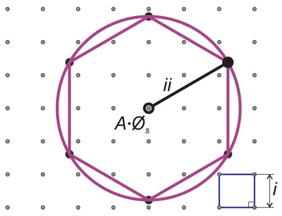
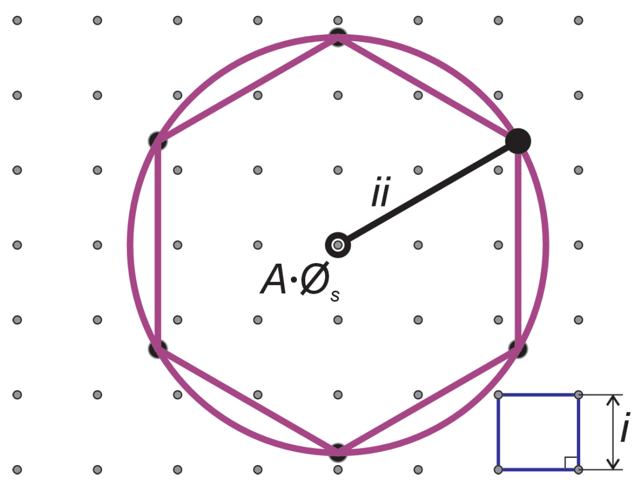
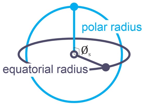
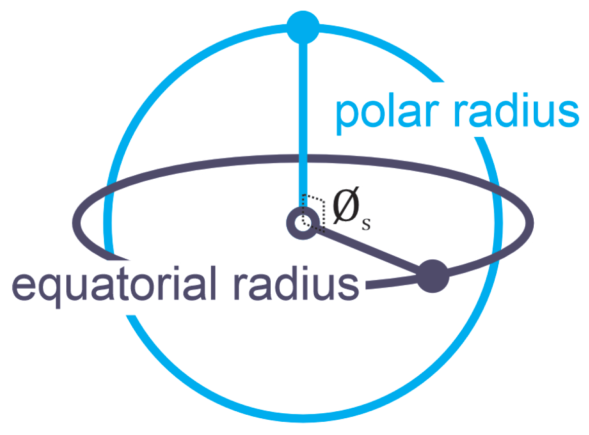
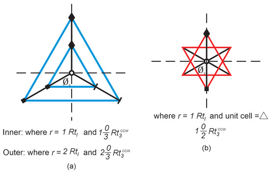
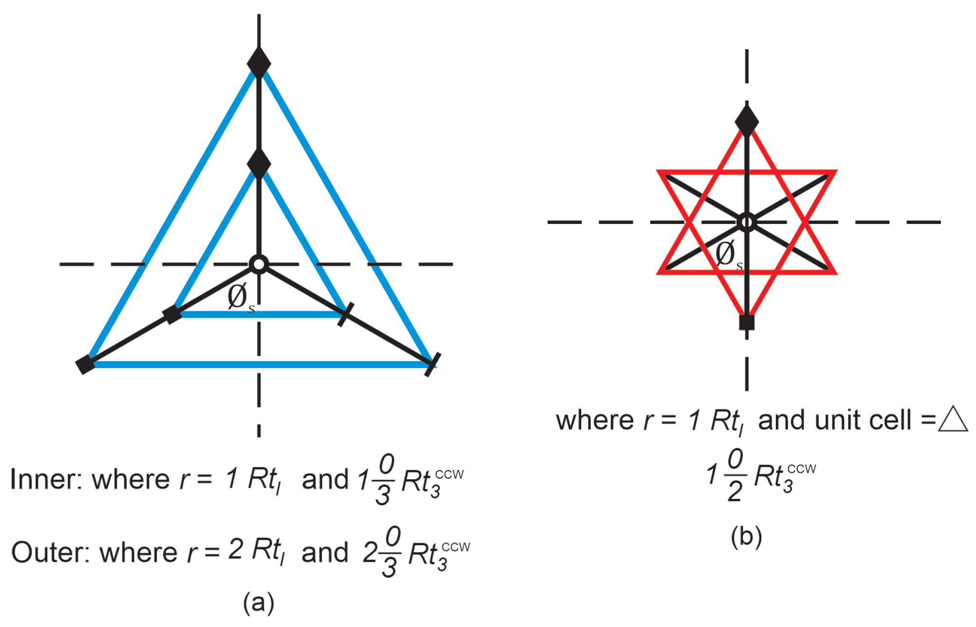
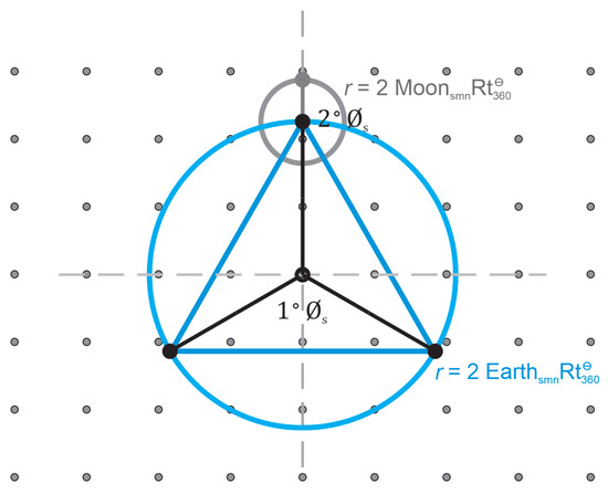
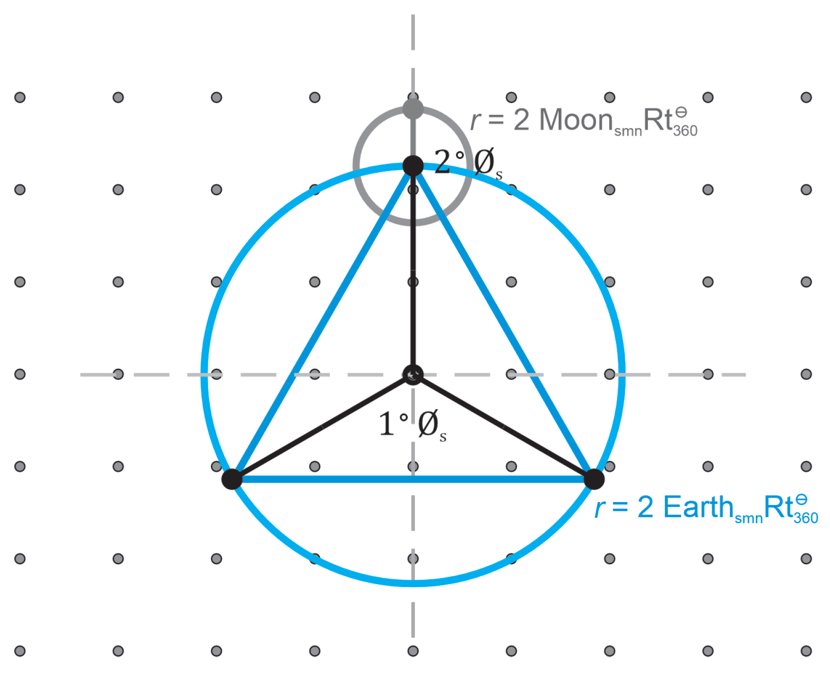
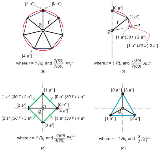
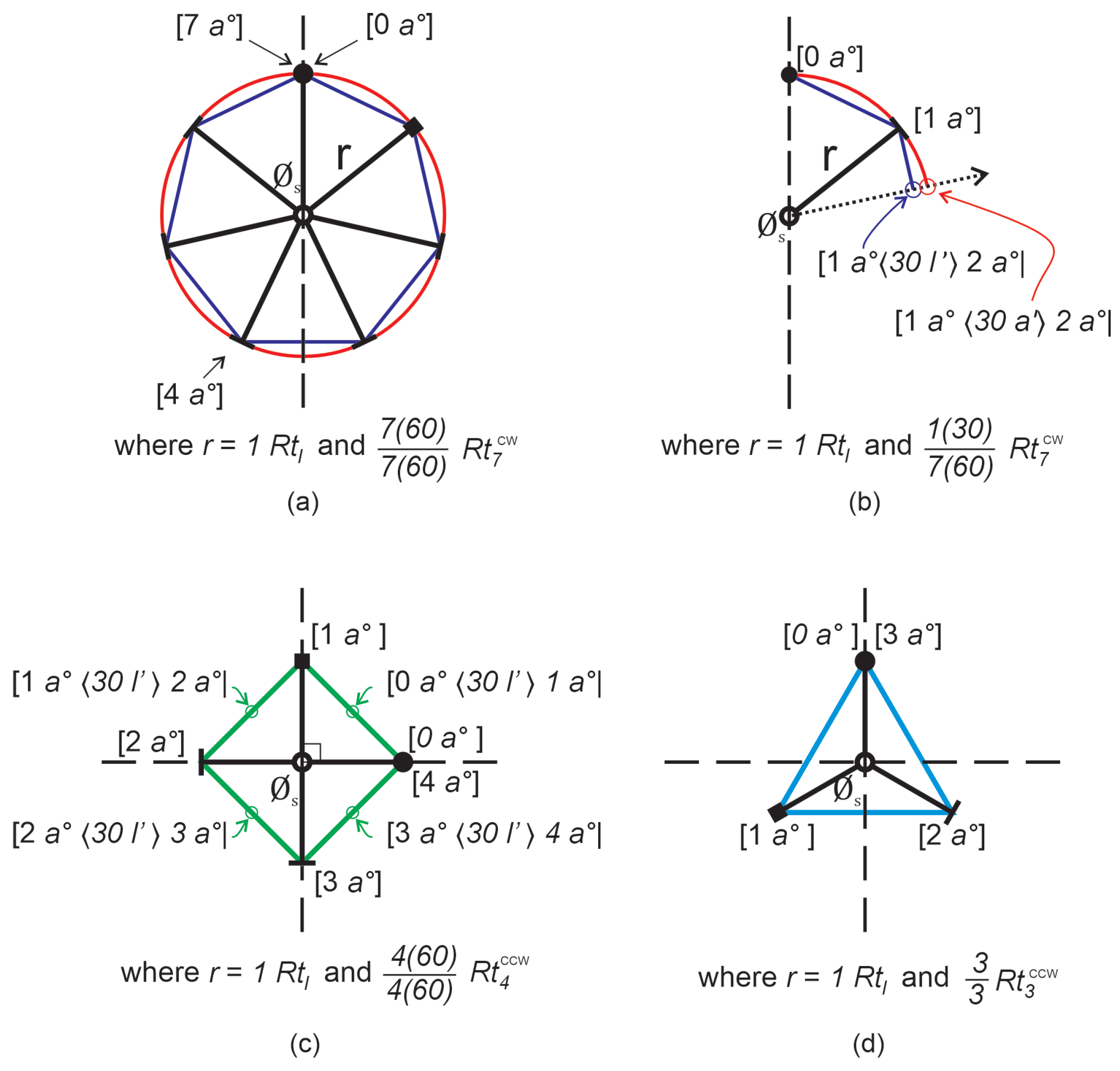
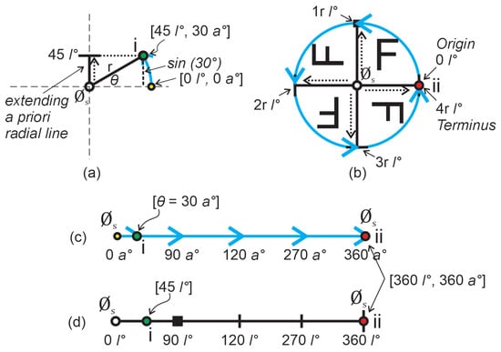
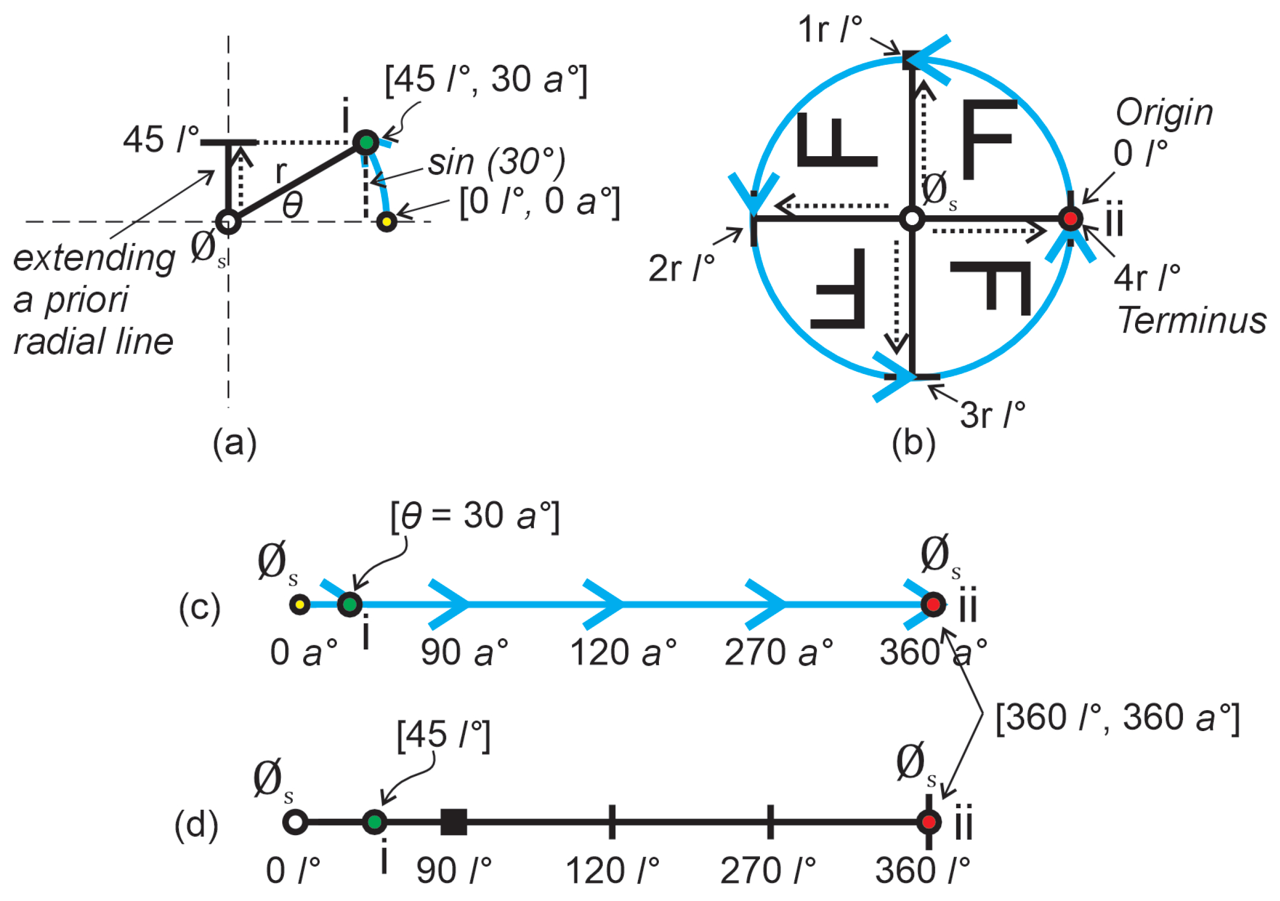
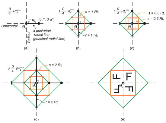
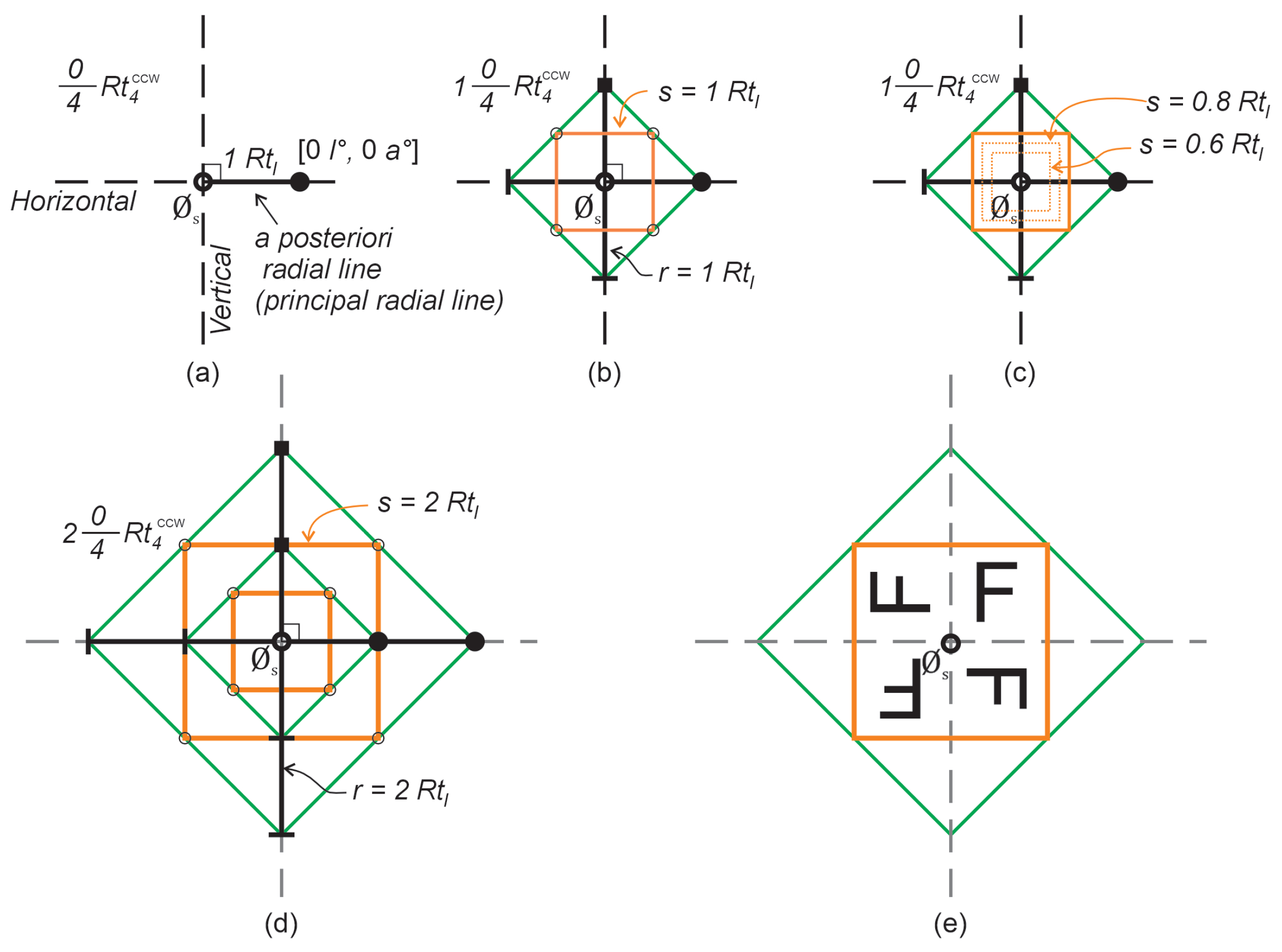
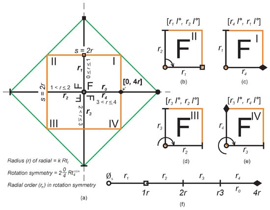
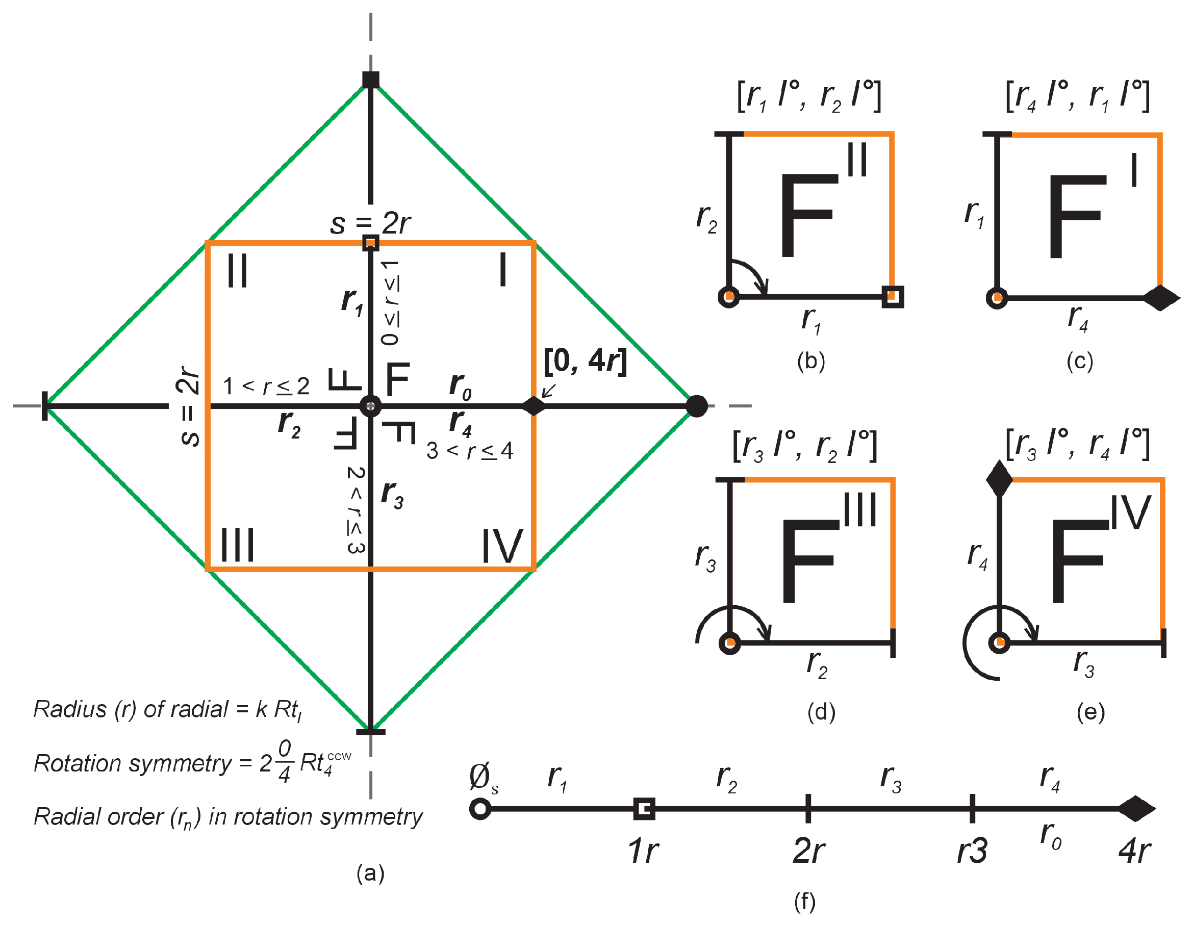
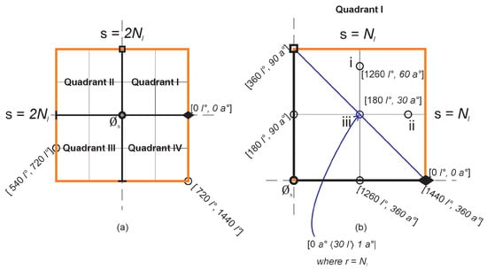
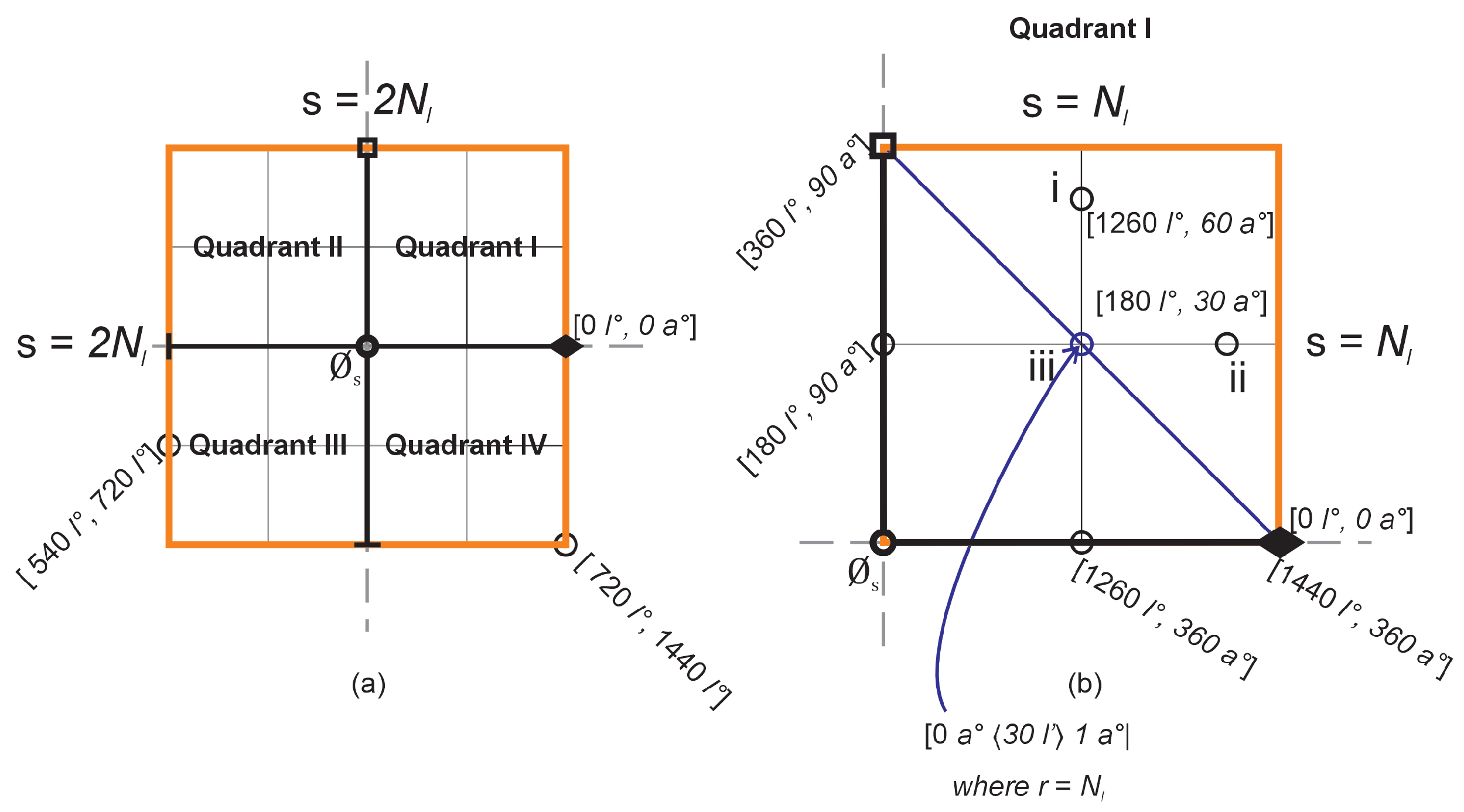
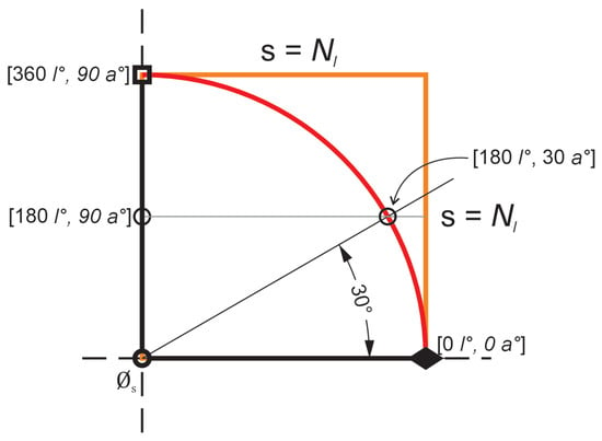
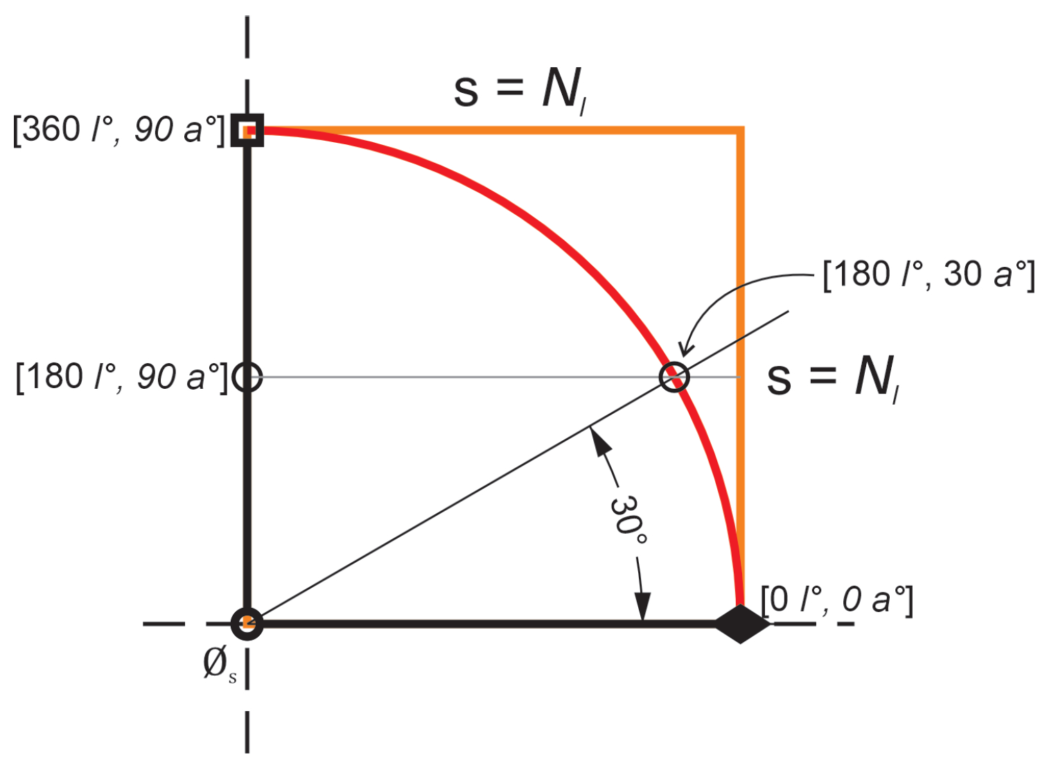
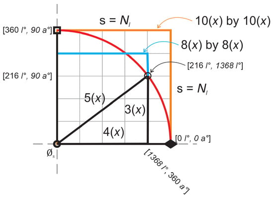
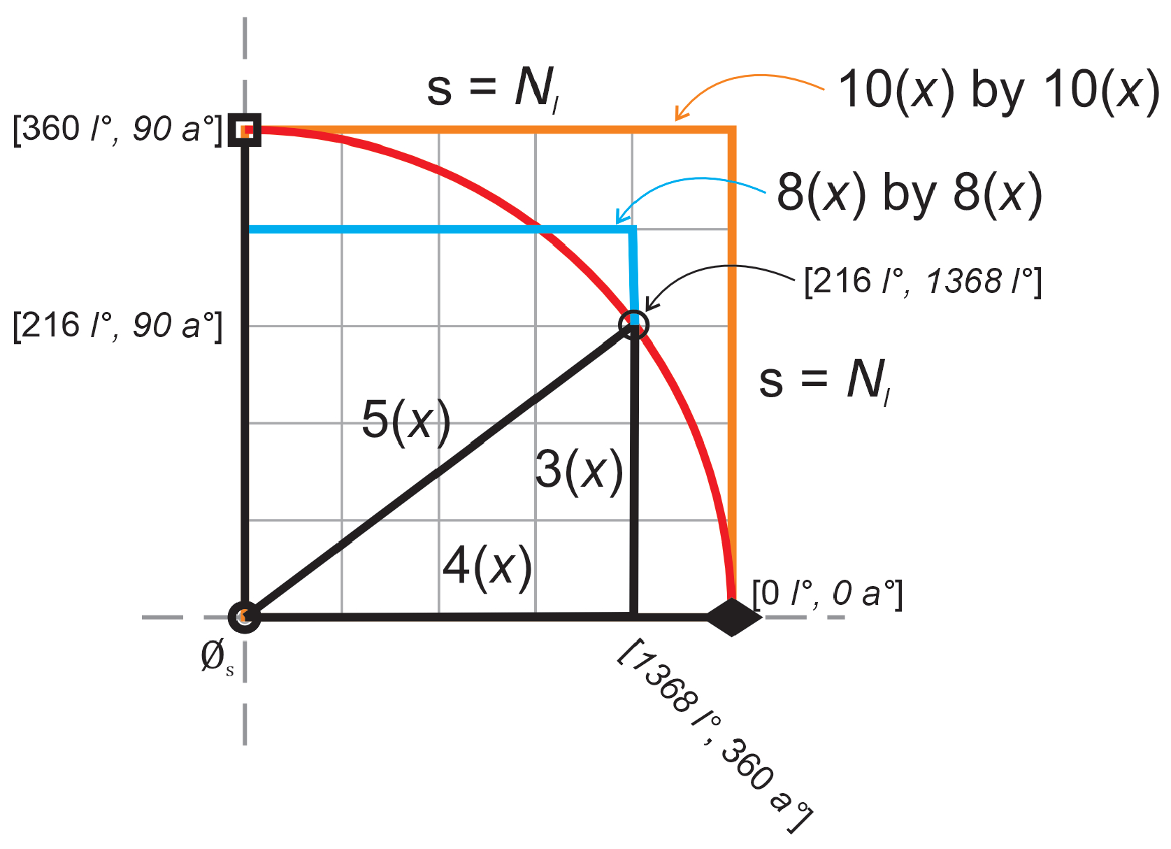
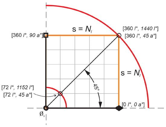
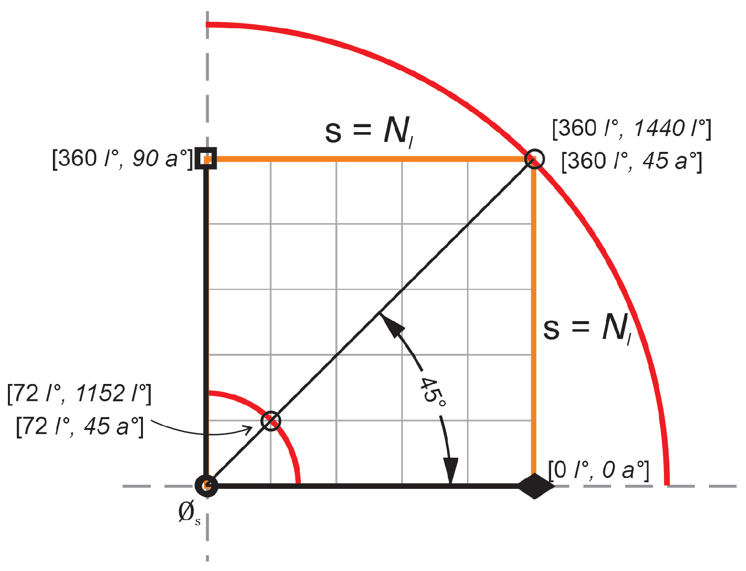
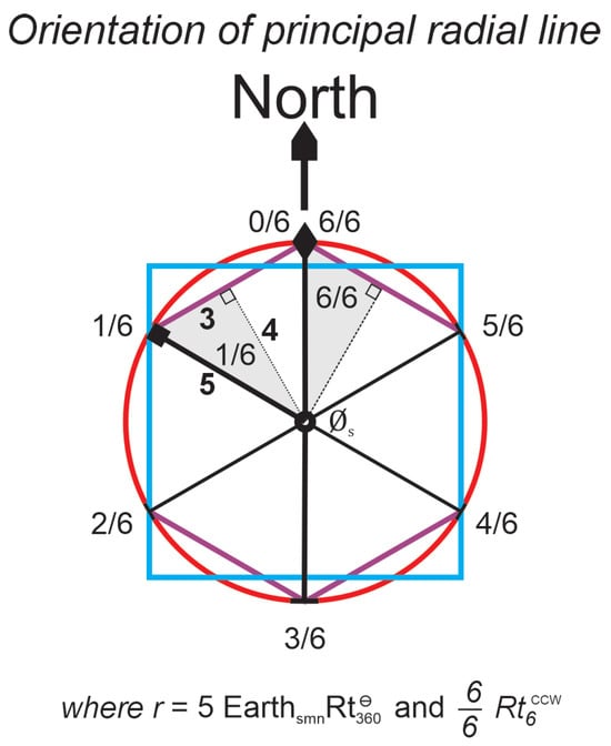
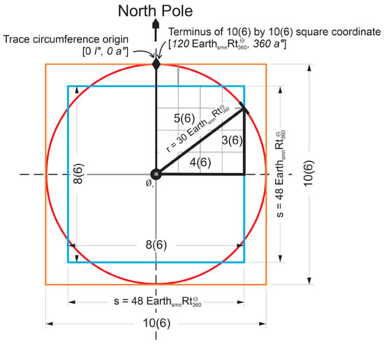
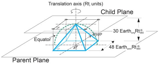
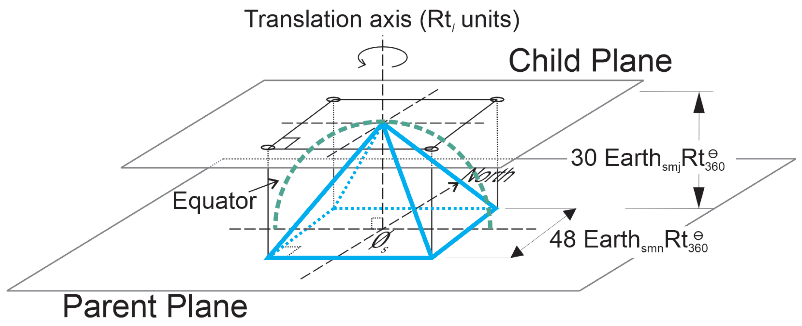

Disclaimer/Publisher’s Note: The statements, opinions and data contained in all publications are solely those of the individual author(s) and contributor(s) and not of MDPI and/or the editor(s). MDPI and/or the editor(s) disclaim responsibility for any injury to people or property resulting from any ideas, methods, instructions or products referred to in the content. |
© 2026 by the author. Licensee MDPI, Basel, Switzerland. This article is an open access article distributed under the terms and conditions of the Creative Commons Attribution (CC BY) license.