


Abstract
Low-rank recovery has emerged as a powerful methodology for the restoration of degraded images. Conventional low-rank recovery techniques, however, predominantly rely on nuclear norm or weighted nuclear norm minimization to separate sparse noise. A significant limitation of this approach is its dependence on full singular value decomposition, which imposes a substantial computational burden, thereby hindering its practical applicability. This paper presents a novel image denoising model integrating the weighted nuclear norm and deep image prior. The weighted nuclear norm is introduced to accurately characterize the global structural properties of images, ensuring the consistency of the overall image structure after denoising. Meanwhile, the deep image prior is employed to effectively capture local details, which helps avoid the blurring of textures and edges often caused by excessive noise removal. The complementary advantages of the two components enable the proposed model to achieve superior performance compared with existing denoising methods. To efficiently compute the proposed model, we design the bilinear factorization method and the alternating direction method of multipliers. Experiments show that the proposed method outperforms mainstream approaches in both restoration accuracy and computational efficiency, exhibiting rapid convergence and robust algorithm stability, thereby demonstrating excellent comprehensive performance.
1. Introduction
Image restoration has long been a crucial problem in the field of image processing, serving as a vital guarantee for subsequent image analysis and applications. With the effective application of sparse representation theory in image restoration, image restoration methods have witnessed significant advances. As an extension of sparse representation in the matrix domain, low-rank matrices have also been successfully applied to image restoration problems. Low-rank matrix recovery, which estimates low-dimensional structures from degraded observations, forms the theoretical basis for many modern image processing algorithms. Among related studies, principal component analysis (PCA) proposed by Ezequiel et al. [1] is a classic technique. It achieves this by finding an optimal low-rank approximation of the original data, which effectively removes noise while preserving essential features. However, traditional PCA methods rely on strong assumptions about noise types (e.g., Gaussian noise). When there are significant outliers or non-Gaussian noise in the data, their restoration performance and robustness will decrease significantly. To address this limitation, Lin et al. [2] proposed the robust principal component analysis (RPCA) model, which explicitly decomposes the data matrix into the sum of a low-rank structural component and a sparse noise component. This decomposition strategy greatly enhances the robustness of the model. To address the NP-hardness of solving RPCA caused by the non-convex and discontinuous rank function, Candès et al. [3] transformed it into a tractable convex optimization problem. Nevertheless, these models apply a uniform penalty to all singular values. This approach tends to over-shrink large singular values while under-penalizing small ones, which often results in blurred structures and a loss of fine texture details. To tackle this issue, Gu et al. [4] recognized that different singular values of a matrix are not equally important and proposed the weighted nuclear norm minimization model (WRPCA). By assigning smaller penalty weights to larger, more important singular values, this method can approximate the true rank of the matrix more accurately than the traditional nuclear norm, thereby achieving better detail preservation in tasks such as image restoration. This series of studies has laid a solid foundation for low-rank matrix recovery.
The above models based on nuclear norm minimization are theoretically powerful. However, their reliance on repeated singular value decomposition (SVD) for large-scale matrices results in high computational costs. To address this, bilinear factorization has been introduced as an efficient alternative for low-rank recovery [5,6]. However, bilinear factorization methods also bring new challenges. Their objective functions are inherently non-convex, which makes the algorithms prone to being trapped in locally optimal solutions. Especially when observed data are severely missing or contaminated, it is difficult to guarantee the stability and robustness of restoration performance. To address this issue, Shang et al. [7] attempted to combine bilinear factorization with a more refined low-rank measure (the Schatten- norm). Nevertheless, such methods are only applicable to specific parameters like () and (). While the method in [8] constructs a more unified factorization framework, the corresponding Schatten-norm minimization problem struggles to ensure global convergence when . Moreover, closed-form solutions exist only in a few special cases, and most scenarios still rely on high-cost iterative optimization. This indicates that bilinear models based on the Schatten- norm face inherent challenges in terms of parameter adaptability and computational reliability.
In recent years, supervised deep learning methods have effectively learned the complex nonlinear mapping between degraded and clean images using deep neural networks with high representational capacity, achieving breakthrough progress in the field of inverse problems, such as image super-resolution, denoising, and reconstruction [9,10,11,12,13,14,15]. For instance, supervised or semi-supervised methods based on vision–language models like CLIP have demonstrated strong cross-modal understanding and generalization through pre-training on large-scale image–text pairs [11,12]. However, the success of such methods heavily relies on the support of large-scale high-quality paired datasets. When such data become scarce due to the high annotation cost [13], the model’s performance and generalization ability degrade notably [14,15]. This causes significant obstacles in their application to fields with scarce annotated data, such as medical imaging and remote sensing. Especially in practical industrial scenarios, building comprehensive annotated datasets is often costly and has limited feasibility [16]. To alleviate this issue, researchers have begun to explore combining powerful pre-trained vision–language models with prompt learning, aiming to achieve better knowledge transfer under limited annotations [17,18,19]. Latest studies, such as TP-OWSSL [20], have effectively improved the model’s discriminative ability in open-world semi-supervised scenarios by introducing global–local text prompt learning strategies and forward–backward strategies. This provides new insights for enhancing model performance under the condition of limited annotated data. However, this only serves to alleviate the issue, and data scarcity remains a major problem. Recent works in image dehazing have explored the role of priors from different perspectives. For instance, IHDCP [21] introduces an explicit haze density correction prior within a physically based model, while FPGDN [22] learns a fuzzy prior via generative adversarial networks to guide the dehazing process. These studies emphasize the critical role of structured priors in dehazing, thereby reinforcing the validity of our approach to fusing low-rank and deep image priors. This principle of complementary information fusion is also reflected in other vision tasks. SCAFNet [23] adaptively fuses CNN and Transformer features for change detection, and PISENet [24] progressively integrates multi-scale features with saliency guidance for salient object detection—both resonating with our strategy of combining global structural priors with local detail priors for image denoising. Similarly, SETR-Net [25] shows that a well-designed single-feature enhancement can outperform complex multi-scale fusion in video saliency prediction, echoing our emphasis on efficient yet effective model design.
To break through this bottleneck, researchers have turned their attention to unsupervised learning paradigms [26,27,28]. Among these, deep image prior (DIP) has opened up a new pathway for image restoration by revealing the implicit regularization properties inherent in the architecture of untrained convolutional neural networks [29]. This framework enables high-quality reconstruction by merely fitting the degraded image itself with the network, without requiring any external training data. To further expand the performance of DIP, scholars have conducted a series of improvement studies [30,31,32]. In particular, Liu et al. were the first to combine the traditional total variation (TV) prior with DIP [33], enhancing the stability of reconstructed structures—this approach has been further verified in X-ray imaging and CT reconstruction [34,35]. Mataev et al. innovatively introduced denoising regularization (RED) into the DIP framework [36,37], improving denoising performance by establishing explicit image priors. The spatially adaptive TV regularization method proposed by Cascarano et al. [38] adaptively modulates local smoothing constraints. To address the need for detail preservation, Xu et al. [39] integrated the low-rank priors, RED with DIP, achieving excellent performance. Additionally, the introduction of vector bundle TV has expanded the application of DIP in color image restoration [40], while the Dual-DIP framework proposed by Gandelsman et al. [41] has provided new insights for multi-layer image decomposition. Later, the adaptive regularization strength estimation model proposed by Cascarano et al. [42] further enhanced the robustness of the method. Despite the significant achievements of these improvements, the restoration accuracy and stability of existing DIP-based methods in complex degradation scenarios still fail to fully meet practical requirements. How to more effectively fuse explicit and implicit priors remains a key issue worthy of in-depth exploration. To further improve DIP’s performance, Chen et al. [43] recently leveraged the low-rank prior and deep image prior, proposing the reweighted low-rank matrix factorization with deep prior (RMFD) model. This model successfully handles images contaminated by salt-and-pepper noise, achieving both theoretical breakthroughs and computational efficiency. Although the RMFD model effectively integrates the low-rank prior and the deep image prior, its design based on the -norm data fidelity term makes it primarily suitable for salt-and-pepper noise. However, in real-world imaging scenarios (such as low-light photography, medical imaging, and remote sensing), images are often corrupted by mixed noise, where Gaussian noise (caused by sensor thermal fluctuations) and salt-and-pepper noise (caused by transmission errors or faulty pixels) coexist. This type of mixed noise is particularly challenging because it combines dense low-amplitude noise with sparse high-amplitude outliers, rendering methods designed for single noise types ineffective. Consequently, developing a model capable of jointly handling both noise types is not only a theoretical necessity but also a practical requirement for robust image restoration. In contrast, our model introduces an -norm data fidelity term to characterize Gaussian noise, thereby modeling sparse salt-and-pepper noise and dense Gaussian noise separately, and extending the applicable scenario from single noise to mixed noise degradation. More importantly, the two priors exhibit intrinsic complementarity that aligns naturally with the characteristics of mixed noise. The reweighted nuclear norm performs well in preserving the global low-rank structure (e.g., smooth regions and main contours) by enforcing low-rank constraints on the entire image matrix. This makes it an effective strategy against dense but low-amplitude Gaussian noise. However, when applied alone, it tends to over-smooth fine textures and edges. Conversely, the deep image prior (DIP) implicitly regularizes the network architecture to reconstruct local details and textures, making it well-suited for recovering regions corrupted by sparse high-amplitude outliers (i.e., salt-and-pepper noise). Yet, DIP alone may struggle to maintain global consistency across the entire image. In RMFD, the use of only the -norm prevents the complementary strengths of these two priors from being fully realized, as the model cannot effectively decouple the two noise types. By introducing the -norm data term, our model explicitly separates Gaussian noise from salt-and-pepper noise. This decomposition enables a specialized division of labor. The reweighted nuclear norm focuses on preserving global structural fidelity, while the deep image prior concentrates on generating local details. Consequently, each prior addresses the noise type it is best suited for. This combination of the two priors, enabled by the mixed noise decomposition mechanism, constitutes the core novelty and advantage of our model over existing methods, such as RMFD.
Based on these, this paper proposes a new image restoration model leveraging a low-rank and deep image prior. Specifically, this new model consists of three components: a low-rank component, a sparse component, and an error term. The low-rank term captures the global structure of images. The sparse term describes the salt-and-pepper noise. The error term characterizes Gaussian noise. To enhance the capture of local image details, the deep image prior is introduced as a key component into the proposed denoising model. By utilizing a low-rank prior and deep image prior, the model achieves simultaneous separation and handling of Gaussian–salt-and-pepper mixed noise, further enhancing the modeling capability for complex degraded data. Compared with RMFD, the new model can separate Gaussian and salt-and-pepper noise simultaneously. Experiments have demonstrated that our model achieves better results for degraded images with Gaussian–salt-and-pepper mixed noise. The main contributions of this paper are summarized as follows:
- A mixed noise separation model integrating low-rank and deep image prior is proposed. The restoration mechanism employs two complementary priors: a low-rank prior for modeling global image structure and correlations, working in concert with a deep image prior that reconstructs local details and textures. These two terms complement each other’s advantages, significantly enhancing the overall capability to characterize the intrinsic structure of images.
- For more efficient computation, we introduce bilinear factorization to convert the original model into an equivalent yet more manageable form. On this basis, we adopt the framework of the alternating direction method of multipliers (ADMMs) to decompose the complex joint optimization problem into a series of efficiently solvable subproblems, thereby significantly improving the computational efficiency and stability of the algorithm.
- Extensive experiments show that our model significantly outperforms state-of-the-art methods in both visual quality and objective metrics.
The remainder of this paper is organized as follows: Section 2 introduces the related works that are closely associated with the model proposed in this paper. Section 3 presents our proposed model and provides the algorithm for solving this new model. Section 4 describes the numerical experimental setup, comparative experimental results, and ablation experiments for the model. Section 5 presents the conclusions.
2. Related Work
We let be an matrix. In practical problems, such matrices often exhibit a low-rank property, which is a key characteristic for subsequent analysis. However, during data acquisition, often contains some noise, which can destroy its inherent low-rank property. To restore the original low-rank structure, Ezequiel et al. [1] proposed the PCA method. This method decomposes the original data into the sum of a low-rank matrix and a noise matrix . Specifically, it works as follows:
where denotes the input original data matrix, represents a noise interference matrix with small element values and follows a Gaussian distribution, stands for the rank of the low-rank matrix , and is a given number.
However, principal component analysis (PCA) is sensitive to significant outlier noise, often leading to lower accuracy and robustness. Furthermore, PCA requires the latent dimensionality to be determined in advance, which is often impractical in real-world applications.
To overcome these challenges, Lin et al. [2] proposed the RPCA model using compressed sensing. RPCA works by decomposing the data matrix into a low-rank matrix , which represents the data’s structural information, and a sparse matrix , which accounts for the noise. Through this method, RPCA can effectively restore structural information even with heavy outlier noise. It not only offers stronger robustness but also removes the burden of presupposing the dimension. We formulate the RPCA optimization problem as:
where is the input original data matrix, is a sparse noise matrix, denotes the -norm of a matrix, and is a weighting parameter. The non-convex and discontinuous nature of the rank function makes Equation (2) an NP-hardness problem to solve. In their seminal work, Candès et al. [3] thus relaxed this non-convex problem into a convex formulation, presented below:
where represents the structural information, represents the sparse noise, stands for the nuclear norm of a matrix, and stands for the -norm of a matrix.
As research in relevant fields gradually deepens, researchers have discovered that using a weighted nuclear norm to replace the nuclear norm produces better results. This is because it does not simply assume that all singular values in a matrix are equally important; on the contrary, the weighted nuclear norm assigns different weights to different singular values, and these weights can be adjusted adaptively. Such a setup can reflect the differences among image data. Based on this concept, Gu et al. [4] replaced the nuclear norm in (3) with a weighted nuclear norm and constructed a model optimizing WRPCA. The specific model is as follows:
Different from traditional deep learning for images, Ulyanov et al. [29] proposed a DIP method. This method utilizes the inductive bias inherent in untrained convolutional neural networks as an image prior. This approach effectively solves various image inverse problems, such as denoising, super-resolution, and inpainting. The model is as follows:
and in the above formula, denotes a CNN generator, is a linear operator, represents a natural image, and is a randomly input vector. The core idea is to model the image as a differentiable function of randomly initialized network parameters. During optimization, the method fits the model using only a single degraded image. Thus, it avoids the dependence on large-scale datasets and has achieved some good results.
However, the implicit prior relied on by DIP has limited constraint capability in complex scenarios. To overcome this limitation, Chen et al. [43], inspired by the DIP framework, integrated the explicit low-rank prior into the model in the form of a reweighted nuclear norm and proposed the RMFD model as follows:
where denotes a mask, is the input original data matrix, and is a regularization parameter. represents a CNN generator, and is a randomly input vector.
To solve the reweighted nuclear norm effectively, we need to employ the bilinear decomposition and the following Lemma 1.
Lemma 1
([44]). Given a matrix , a regularization parameter , and a set of non-decreasing weights , the optimization problem with a weighted Frobenius norm is:
whose solution has the following closed-form expression:
Here, is the diagonal weight matrix, is the singular value decomposition of the matrix , and are, respectively, the left and right singular vectors of , and is the singular value matrix.
3. New Model, Algorithm, and Convergence Analysis
3.1. New Model and Algorithm
The RMFD model demonstrates excellent performance in noise processing by fusing reweighted low-rank factor decomposition with the deep image prior. However, this model adopts the -norm as the data term, which is more suitable for processing images with only salt-and-pepper noise [45]. Nevertheless, actually acquired images often contain a large amount of Gaussian noise. Using only the single -norm fidelity term makes it difficult to remove Gaussian noise, which in turn leads to limited image restoration performance.
To effectively remove complex mixed noise, we propose a new model as follows:
where is the input original data matrix, are regularization parameters, and is called the reweighted nuclear norm of , where is the weight related to the -th singular value of . denotes a CNN generator, and is a randomly input vector. In the new model (8), the first term is the reweighted nuclear norm, which is used to constrain the global structural characteristics of the image, the second term is a sparse error term, describing sparse salt-and-pepper noise, and the third term is a data term that ensures the reconstructed result is consistent with the observed data. This design enables the model to inherit the advantages of low-rank methods in characterizing global structures and the strength of the deep prior in describing local details. These two aspects complement each other, jointly ensuring the high quality of the restored image in both global and local aspects.
Compared with traditional models, the new model (8) contains a deep image prior. This prior utilizes the inherent inductive bias of the convolutional neural network structure and can capture and generate textures and structures that match the statistical laws of natural images from the degraded image itself without relying on a large amount of external data, thus exhibiting significant advantages in restoring local details and edges of images. Compared to the RMFD model, which mainly handles single salt-and-pepper noise, the new model can accurately separate salt-and-pepper noise and Gaussian noise simultaneously by introducing an norm fidelity term for Gaussian noise. It realizes the synchronous processing of sparse noise and dense noise and successfully expands the applicable range from single-noise scenarios to mixed noise degradation environments.
Next, we will give the resolving algorithm for the new model. Equation (8) incorporates a reweighted nuclear norm. Direct application of singular value decomposition is computationally expensive, making it hard to extend to large-scale problems [41]. To improve computational efficiency, this paper adopts a bilinear factor decomposition strategy [18]. Let , where and are two low-rank factor matrices, and is a given value. Then, the decomposition form is as follows:
Using Equation (9), Equation (8) can be turned into:
and for Equation (10), let . Then, the augmented Lagrangian function is obtained as follows:
where are all Lagrange parameters, and is a positive scalar, referred to as penalty parameters.
By applying the ADMM to Equation (11), given the initial values of the optimization parameters and the iteration step , the update formulas for at the iteration step can be obtained:
For Equations (12) and (13), by computing the Gateaux derivatives with respect to and , respectively, the closed-form solutions, i.e., Equations (21) and (22), are obtained as follows:
For Equations (14) and (15), according to Lemma 1, we have
and among them, is a diagonal weight matrix, , the regularization parameter , and are, respectively, the left and right singular vectors of , while and are the left and right singular vectors of , respectively.
For Equation (16), we use the Adam optimizer [46] for iteration.
For Equation (17), we use the soft-thresholding method introduced in [47] to solve it, and obtain:
Based on the above discussion, the algorithm for the new model is as follows, which is summarized in Algorithm 1.
| Algorithm 1: The Algorithm Proposed in This Paper |
| Input: Initial values of , and select parameters |
| : |
| Calculate according to (21) |
| Calculate according to (22) |
| Calculate weights for |
| Calculate according to (23) |
| Calculate weights for |
| Calculate according to (24) |
| Calculate according to (16) |
| Calculate according to (25) Calculate the Lagrange parameters , , according to (18), (19), and (20). |
| Output: |
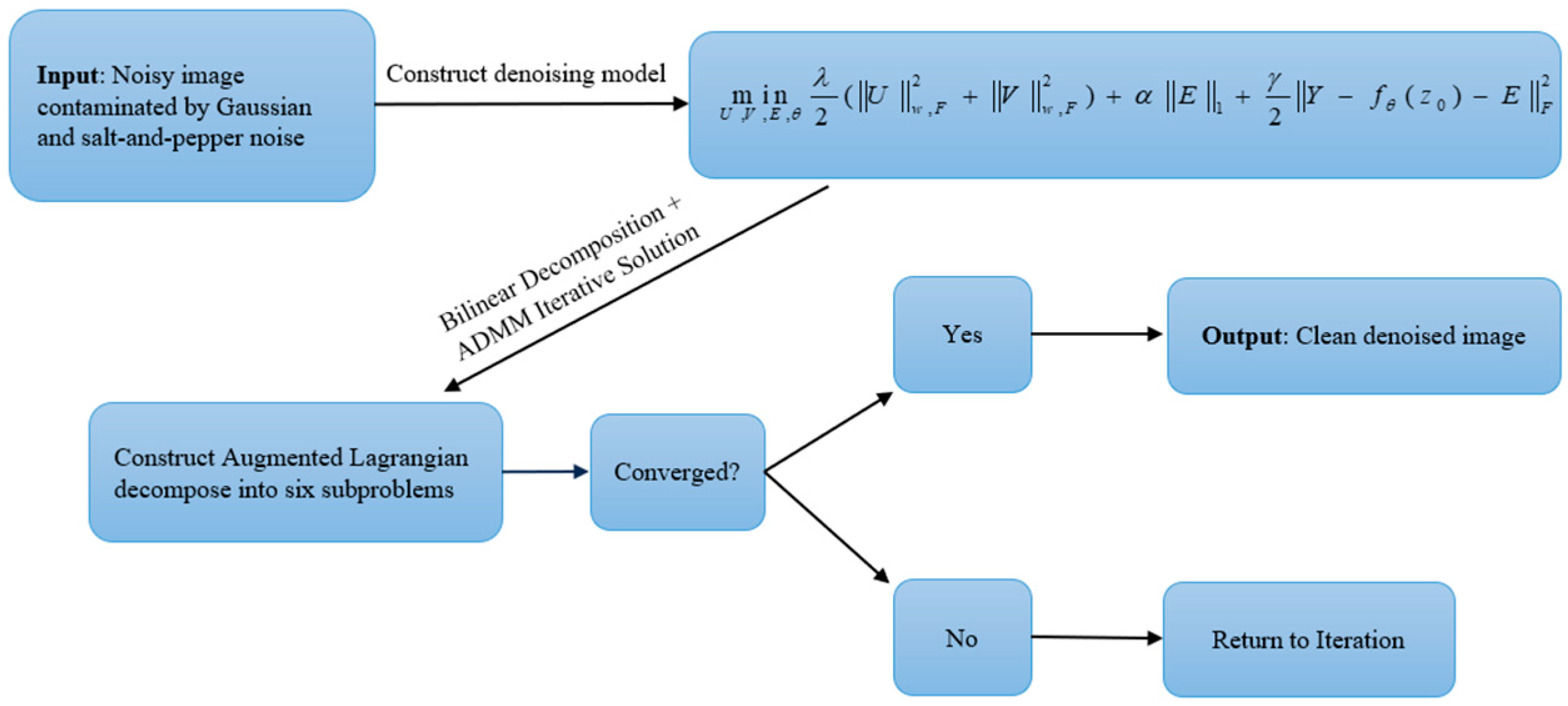
The above analysis and derivations have clarified the optimization objective and solution strategy of the proposed model. To enable readers to intuitively grasp the macro execution logic and data interaction of the algorithm, Figure 1 presents the overall flowchart of our mixed noise removal algorithm. This flowchart modularly depicts the entire pipeline, progressing from input and model construction to augmented Lagrangian decomposition and ADMM iteration until convergence. It also clearly reveals the correspondence between different noise constraint terms and their respective solution steps.
Figure 1.
Flowchart of the proposed mixed noise denoising method.
3.2. Convergence Analysis
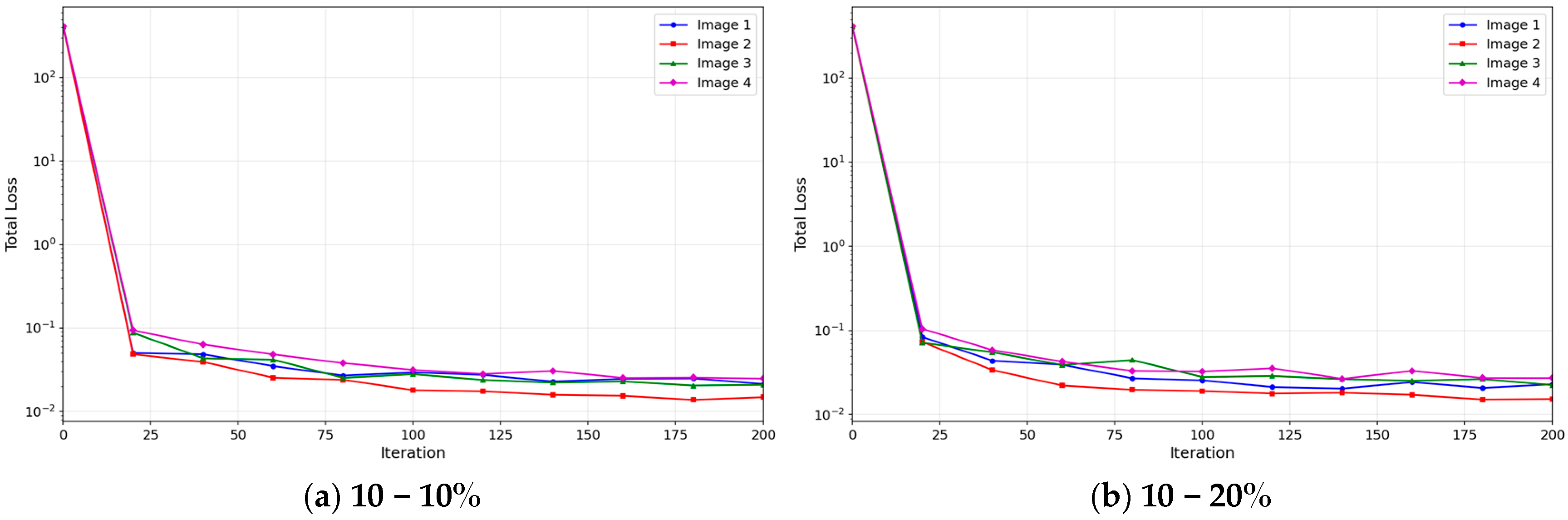
The inherent non-convexity of the reweighted nuclear norm substantially complicates the convergence analysis of algorithms based on the alternating direction method of multipliers (ADMMs). Consequently, most existing approaches utilizing this norm only provide empirical validation or guarantee convergence in a weaker sense [48,49]. Moreover, analyzing the convergence of models with deep priors introduces additional challenges, primarily due to the non-convex components introduced by neural networks. To better verify network convergence, Figure 2 shows the curves of total loss versus iteration number for four test images under two mixed noise conditions, thereby simplifying visualization and highlighting the key convergence behavior. In these figures, the horizontal axis represents the iteration number, and the vertical axis represents the total loss value. In Figure 2a, under the condition of Gaussian noise level 10 and salt-and-pepper noise ratio 10%, all four loss curves exhibit a monotonic decrease and rapidly stabilize, despite differences in image content. Similarly, in Figure 2b, under higher noise intensity (Gaussian noise level 10 and salt-and-pepper noise ratio 20%), the loss curves for all test images maintain a steady downward trend. These results demonstrate that, under the same noise conditions, the proposed algorithm effectively reduces the objective function value for images with varying content. The consistent convergence patterns observed across multiple images under both noise settings intuitively confirm the stability and robustness of the algorithm, showing that it reliably converges to high-quality solutions without significant oscillations. Accordingly, the stable performance observed on different test images further underscores the practical applicability of the proposed model for real-world image denoising tasks.
Figure 2.
Total loss curves versus iteration numbers for four test images under different mixed noise conditions. (a) Loss curves under mixed noise of Gaussian noise level 10 and salt-and-pepper noise ratio 10%; (b) Loss curves under mixed noise of Gaussian noise level 10 and salt-and-pepper noise ratio 20%.
4. Numerical Experiments
In this paper, we verify the effectiveness of the proposed new model in image denoising by presenting the numerical experimental results of the new model and several comparison models, mainly including visualization and quantitative indicators (PSNR and SSIM).
4.1. Network Architecture
In this study, we adopt a symmetric encoder–decoder network adapted from Ref. [43]. The encoder employs a five-level contracting structure, in which feature extraction and downsampling are simultaneously achieved via strided convolutions. Batch normalization (BN) and LeakyReLU activation are applied after each convolutional layer, and 1 × 1 convolutions are used at each level to generate compact skip connection features. The decoder adopts a five-level expanding path that gradually restores spatial resolution through nearest upsampling. The decoder features are concatenated with the corresponding skip connection features from the encoder, followed by batch normalization and standard convolutions to adjust the channel dimensions. Additional 1 × 1 convolutions are adopted to further refine the feature representation, and the final output is generated by a 1 × 1 convolution with Sigmoid activation. This framework uses the encoder to capture global semantic information and the decoder to fuse detailed features for high-precision pixel-level prediction.
4.2. Parameter Selection
In our algorithm, we use the Adam optimizer in PyTorch (version 2.6.0) to solve for the network parameters in subproblem (16), with a learning rate of and inner iterations. We manually tune the parameters to achieve the best results. The key hyperparameters of our model, including the penalty parameter , the sparse noise regularization parameter , and the data fidelity parameter , are carefully adjusted through extensive experiments. Specifically, we perform a grid search over a reasonable range for each parameter to evaluate its impact on denoising performance (measured by PSNR and SSIM). is the penalty parameter in the ADMM framework, controlling the balance between the quadratic penalty term and the constraints in the augmented Lagrangian function. A larger drives the variables to satisfy the equality constraints more quickly, thereby accelerating convergence, but an excessively large value may cause numerical instability or iterative oscillations. A smaller relaxes the constraints, resulting in slower but more stable convergence. When , the parameter can be manually adjusted according to different test images to obtain better results. Parameter controls the strength of the sparse noise term , which models salt-and-pepper noise. A larger imposes a stronger penalty on sparse noise, removing more salt-and-pepper noise; however, if is too large, it may mistakenly suppress true image edges, leading to loss of detail. Conversely, if is too small, it becomes difficult to effectively suppress salt-and-pepper noise. Through experiments, we find that the model achieves a good balance between noise removal and detail preservation when . Parameter is the weight of the data fidelity term , which balances the consistency between the observed data and the reconstruction. A larger emphasizes fidelity to the observed image, helping to preserve details but potentially leaving residual Gaussian noise. A smaller strengthens regularization, leading to stronger denoising at the risk of over-smoothing. Experimental results show that within the range , the model performance is relatively insensitive to ; therefore, we adopt as the default value in most experiments.
4.3. Experimental Results
In all experiments, we uniformly set the rank of the low-rank decomposition to 80, consistent with the comparative model RMFD to ensure experimental fairness. This value is exactly the same as the recommended setting for grayscale images in RMFD [43], which has verified that achieves the optimal balance between global structure representation and computational efficiency for natural images. Meanwhile, since our model integrates low-rank decomposition and deep image prior, where the low-rank component captures global structure and the deep network complements local details, a relatively large can be adopted without introducing noise redundancy. Furthermore, effectively covers the structural information of images with varying texture complexities in the test set, avoiding detail blurring caused by an excessively small . In addition, we employ bilinear factorization instead of full SVD, and does not significantly increase the computational burden while guaranteeing recovery accuracy, with running efficiency still superior to traditional low-rank models relying on full SVD.
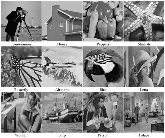
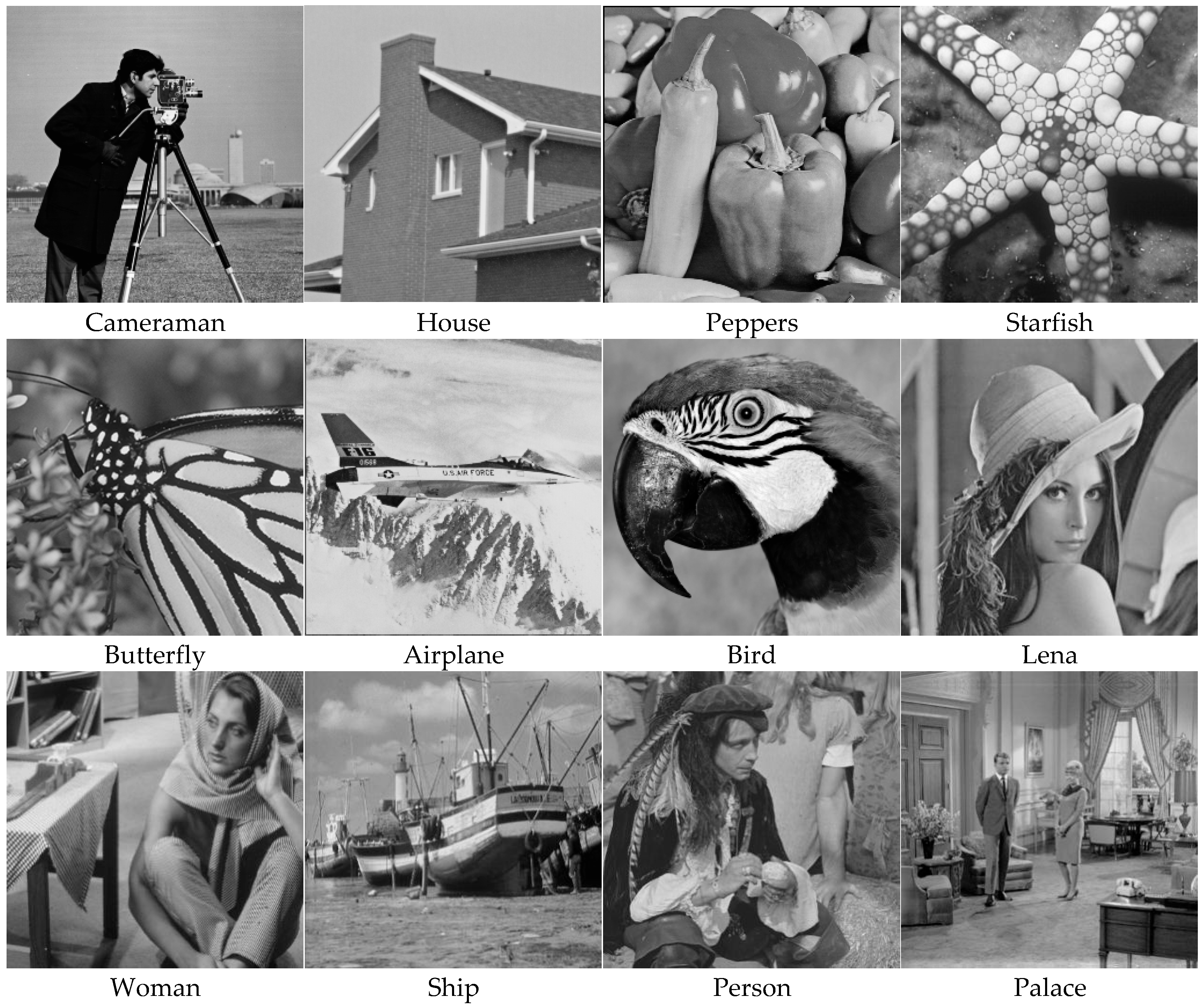
Based on the above configuration, we evaluate our model on the dataset [50] by randomly selecting 12 test images from it, as shown in Figure 3. Gaussian–salt-and-pepper mixed noise is added to the original images, where the standard deviation of Gaussian noise takes values of 10, 20, 30, and 50, and the proportion of salt-and-pepper noise % takes values of 10, 20, 30, 40, and 50. To validate the performance of the proposed model, we select WRPCA [4], DIP [29], RMFD [43], and EN-CNN [51] as comparison methods. To ensure that all comparison methods achieve satisfactory results across different image scenarios, the parameters of each method are carefully tuned multiple times: after initializing the parameters, they are adjusted according to the restoration performance of the test images until the evaluation metrics no longer increase with further parameter changes.
Figure 3.
Test images.
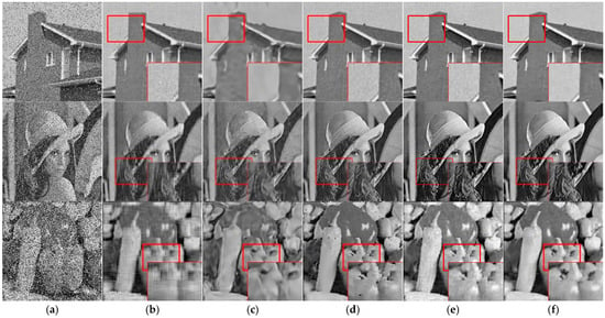
Figure 4 presents the denoising results of different methods under Gaussian noise . The three rows from top to bottom correspond to salt-and-pepper noise ratios of 10%, 20%, and 40%, respectively. The columns from left to right represent different images or processing methods, i.e., (a) noisy image, (b) WRPCA result, (c) DIP result, (d) RMFD result, (e) EN-CNN result, and (f) our proposed model result. For a clear demonstration of the denoising effect, zoomed-in views of the red regions are shown. It can be observed that the WRPCA results suffer from significant loss of texture details and contain many artifacts. The DIP results are overly smooth, lack texture details, and exhibit numerous artifacts, making the images appear unrealistic. The RMFD model performs well in removing salt-and-pepper noise but shows limited effectiveness in suppressing Gaussian noise. As the proportion of salt-and-pepper noise increases (e.g., in the Lena image), fine texture details (such as hair) are lost and edges become blurred. The EN-CNN method, while capable of removing some noise, still leaves noticeable noise in detailed regions (e.g., the House image), leading to suboptimal recovery performance. In contrast, the proposed model effectively removes both salt-and-pepper and Gaussian noise while preserving more texture details, yielding results closer to the original images. To save space and facilitate fair comparison, the PSNR and SSIM values of the restored images by different algorithms are reported in Table 1. The results show that the proposed model consistently outperforms the other methods across most evaluation metrics, demonstrating its excellent denoising capability.
Figure 4.
Denoising results of different models for = 10. (a) input images corrupted by mixed noise; (b) denoising results of the WRPCA method; (c) denoising results of the DIP method; (d) denoising results of the RMED method; (e) denoising results of the EN-CNN method; (f) denoising results of the proposed method. The red boxes in the bottom-right corners show enlarged views of local details.
Table 1.
Denoising index values of different models for = 10.
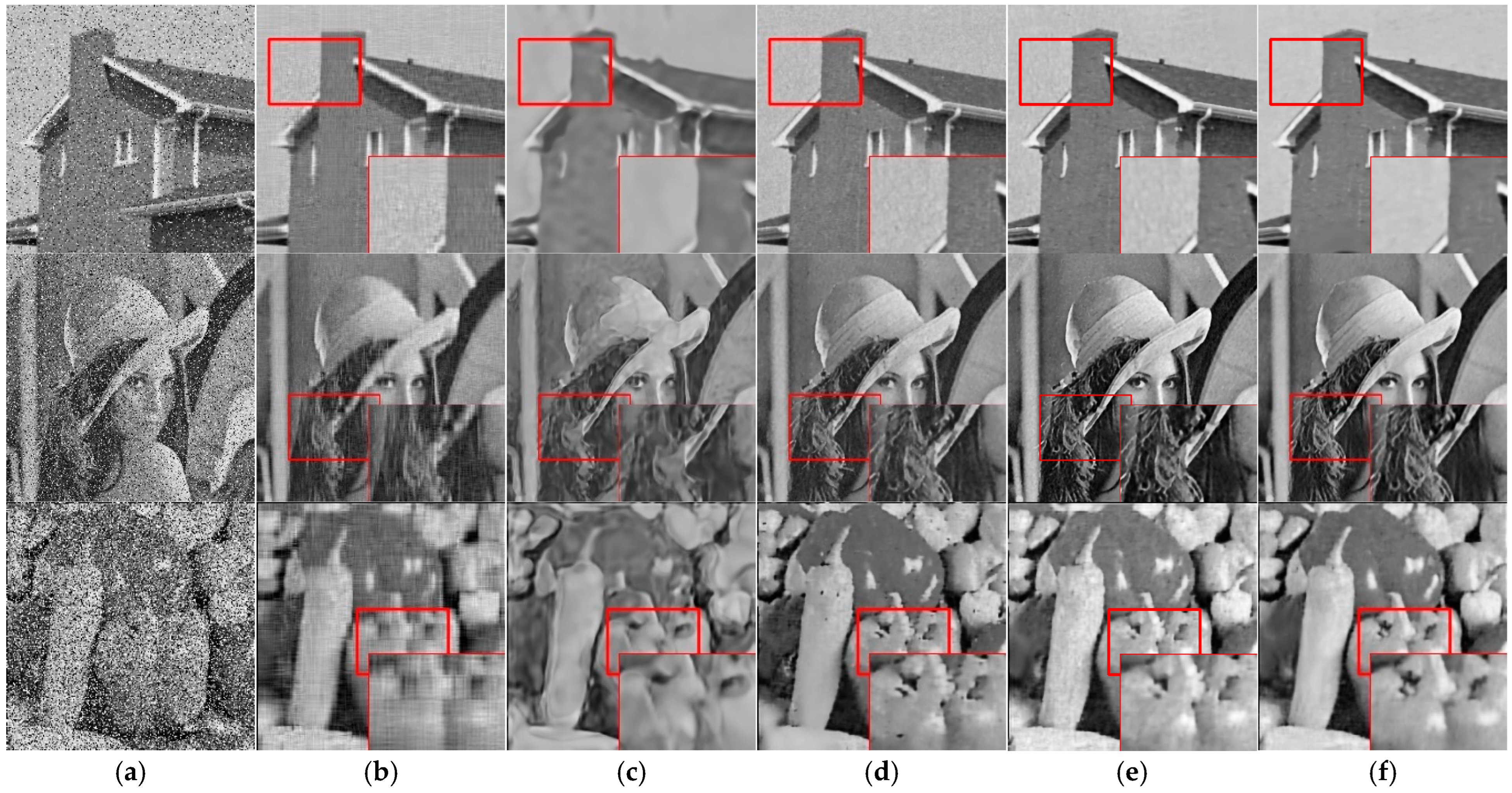
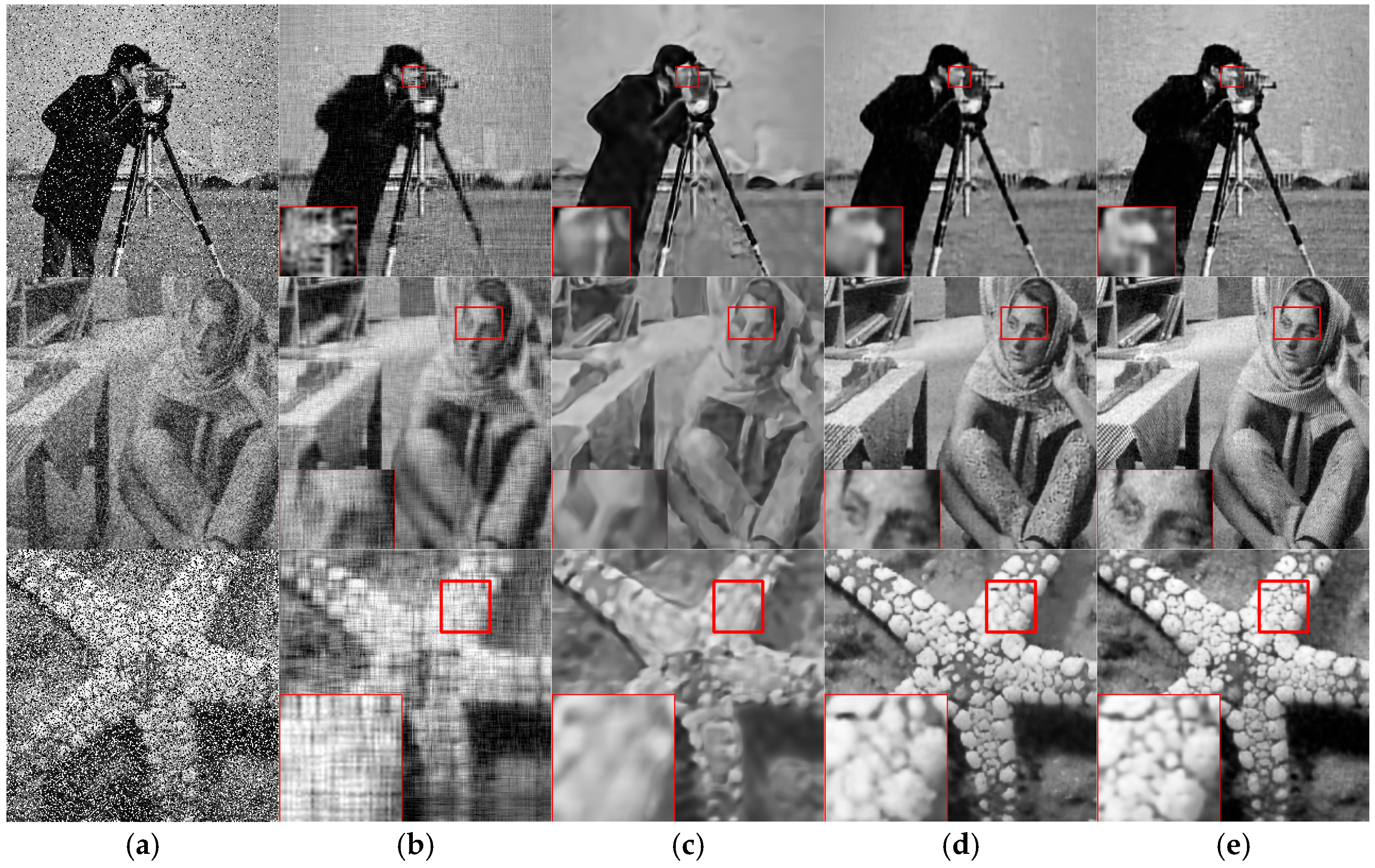
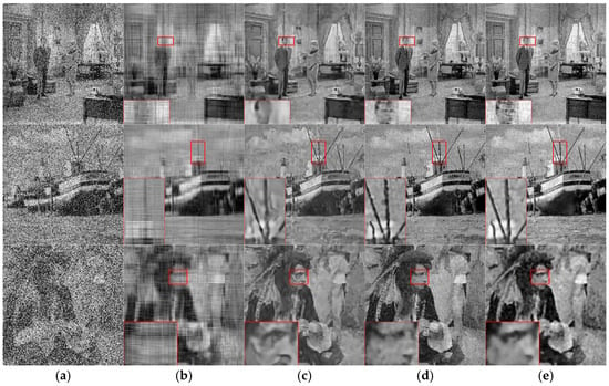
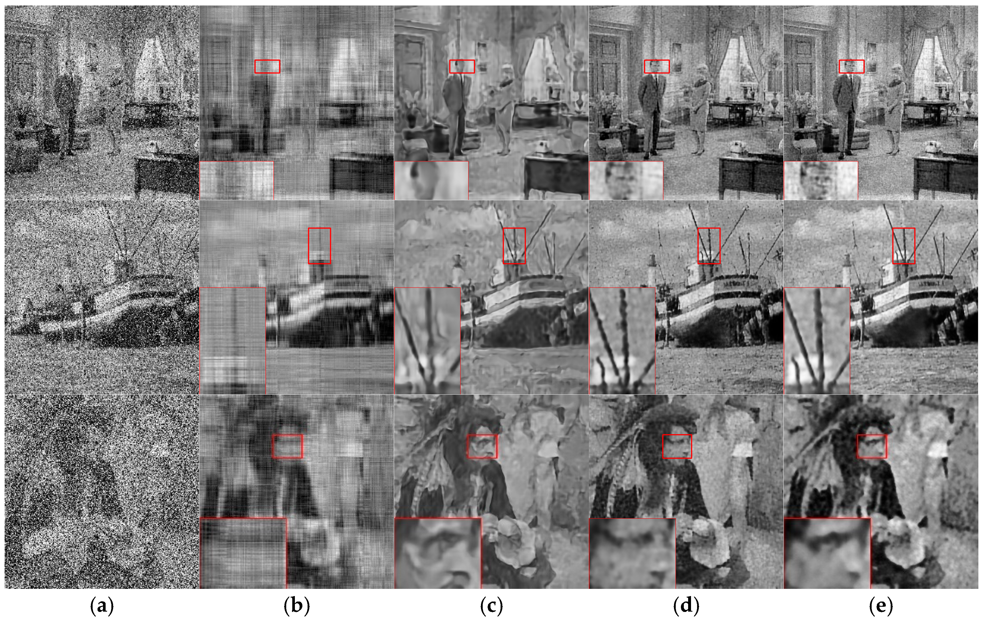
Figure 5 shows the denoised images of different processing methods under Gaussian noise 20. Each row represents different intensities of salt-and-pepper noise, which are 10%, 30%, and 40% from top to bottom. Each column represents different images or processing methods, namely, (a) noisy image, (b) WRPCA result, (c) DIP result, (d) RMFD result, and (e) new model result, from left to right. As can be clearly observed from the zoomed-in red regions, the WRPCA results suffer from severe loss of overall texture information and poor restoration of structural details, leading to significant distortion. The DIP results are over-smoothed, losing substantial texture information, which results in blurred structures and edges. Although the RMFD results retain more texture details than the former two, they fail to completely remove all Gaussian noise, causing some edge blurring. In contrast, the proposed model demonstrates superior performance in both preserving texture information and removing mixed noise compared to the other three methods. Quantitatively, Table 2 lists the PSNR and SSIM values of the competing models when Gaussian noise is set to 20. The results confirm that the proposed model achieves higher values in both metrics, underscoring its exceptional denoising capability.
Figure 5.
Denoising results of different models when = 20. (a) input images corrupted by mixed noise; (b) denoising results of the WRPCA method; (c) denoising results of the DIP method; (d) denoising results of the RMED method; (e) denoising results of the proposed method. The red boxes in the bottom-left corners show enlarged views of local details.
Table 2.
Denoising index values of different models for = 20.
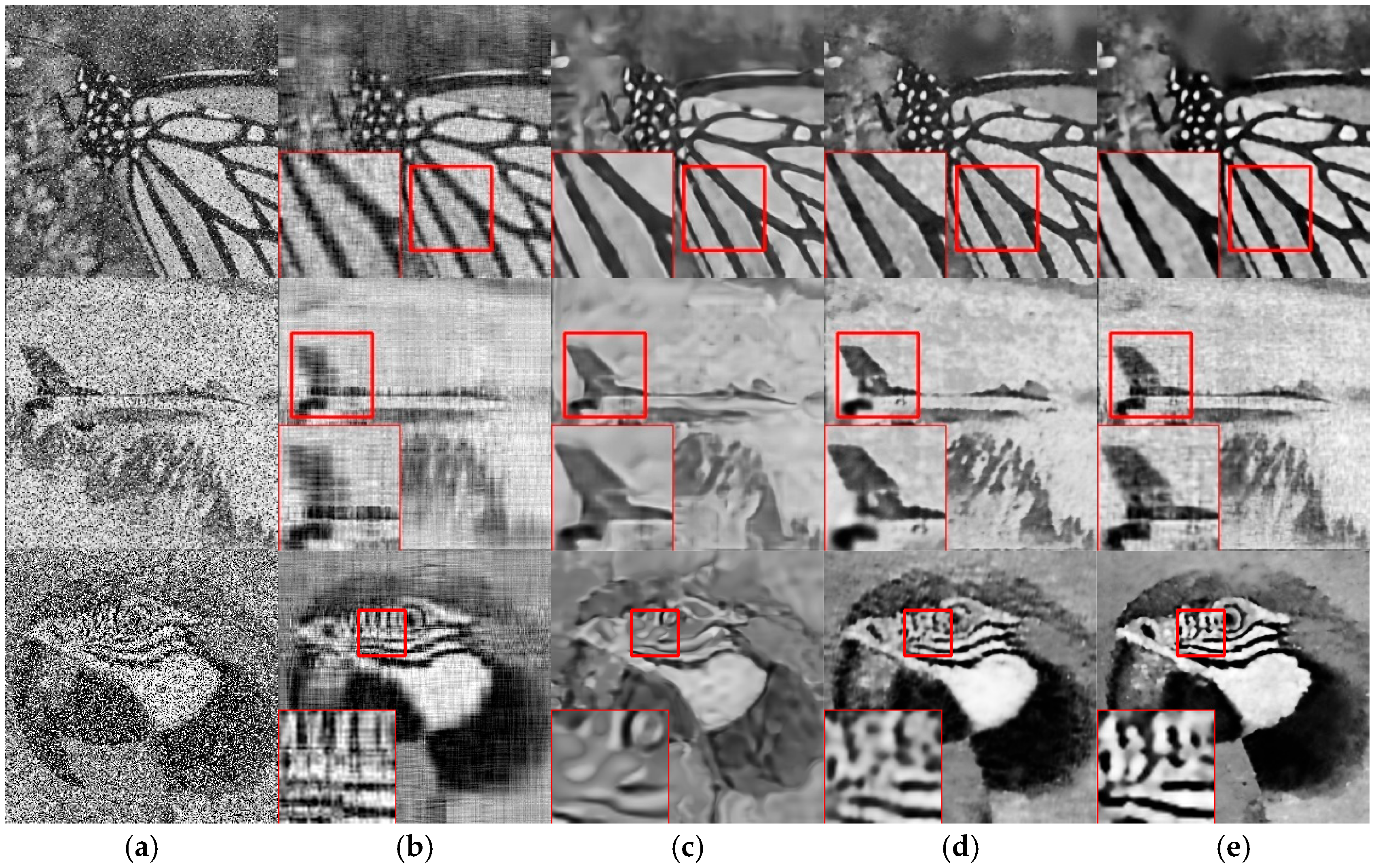
Figure 6 shows the denoised images of different processing methods under the background of fixed Gaussian noise 30. Each row represents different intensities of salt-and-pepper noise, which are 10%, 30%, and 50% from top to bottom. Each column represents different images or processing methods, namely, (a) noisy image, (b) WRPCA result, (c) DIP result, (d) RMFD result, and (e) new model result, from left to right. As evidenced in the zoomed-in red regions, the WRPCA results retain a significant amount of noise while suffering from substantial texture loss during denoising. The outcomes from DIP exhibit excessive smoothing, which not only causes edge deformation but also removes critical texture information, resulting in visible image distortion. Although the RMFD results effectively suppress salt-and-pepper noise, they incompletely remove Gaussian noise and handle edges inadequately, leading to an overall blurry appearance. In contrast, the proposed model successfully removes mixed noise while preserving texture details more effectively than the other methods. Quantitative results further support these observations. Table 3 lists the PSNR and SSIM values obtained by the competing models on twelve images under a Gaussian noise level of 30. The proposed model consistently achieves superior scores in both metrics, confirming its enhanced denoising performance.
Figure 6.
Denoising results of different models when = 30. (a) input images corrupted by mixed noise; (b) denoising results of the WRPCA method; (c) denoising results of the DIP method; (d) denoising results of the RMED method; (e) denoising results of the proposed method. The red boxes in the bottom-left corners show enlarged views of local details.
Table 3.
Denoising index values of different models for = 30.
Figure 7 displays denoised images from different processing methods under the condition of fixed Gaussian noise 50. Each row corresponds to different intensities of salt-and-pepper noise, which are 10%, 20%, and 50% from top to bottom. Each column stands for different images or processing methods, in the following order from left to right: (a) noisy image, (b) WRPCA result, (c) DIP result, (d) RMFD result, and (e) new model result. At the higher noise level ( 50), the limitations of the comparison methods become more pronounced. The output from WRPCA continues to exhibit noticeable noise residues accompanied by severe texture loss. DIP again yields overly smoothed results, where certain edge structures appear distorted and essential textural information is compromised. RMFD maintains its effectiveness against salt-and-pepper noise but still falls short in fully suppressing Gaussian noise, with inadequate edge processing contributing to reduced overall image clarity. In this challenging scenario, the proposed model demonstrates a more effective balance between noise removal and structural preservation. It achieves thorough suppression of mixed noise while maintaining superior performance in reconstructing textures and sharp edges. These qualitative assessments are corroborated by the quantitative metrics presented in Table 4, which reports PSNR and SSIM values for all methods evaluated on the dataset [50] under Gaussian noise 50. Our model consistently achieves the highest scores in both measures, confirming the robustness and comprehensive superiority of its denoising capability.
Figure 7.
Denoising results of different models when = 50. (a) input images corrupted by mixed noise; (b) denoising results of the WRPCA method; (c) denoising results of the DIP method; (d) denoising results of the RMED method; (e) denoising results of the proposed method. The red boxes in the bottom-left corners show enlarged views of local details.
Table 4.
Denoising index values of different models for = 50.
To further validate the effectiveness of the proposed model, the following are the numerical experimental results of the new model and several comparison models.
To quantitatively evaluate the computational efficiency of the proposed model, we further compare the running time of WRPCA, DIP, RMFD, EN-CNN, and our model under different image sizes and various mixed noise conditions. All experiments are conducted on the same experimental platform. For each noise combination, the tests are repeated multiple times, and the mean values are calculated to ensure the comparability and stability of the results. Each method is configured with its optimal denoising performance parameters, and the corresponding running times are recorded. The detailed runtime results are summarized in Table 5.
Table 5.
Runtime comparison (in seconds) of different models under various image sizes and mixed noise conditions.
As shown in Table 5, for images, when the Gaussian noise standard deviation and the salt-and-pepper noise ratio , the running time of our model is 26.97 s, which falls between that of DIP (21.52 s) and RMFD (79.46 s). Under the condition of and , our model takes 20.65 s, which is lower than DIP (35 s) and RMFD (56.81 s). Under the condition of and , the running time of our model is 17.39 s, significantly lower than DIP (23.67 s) and RMFD (45.74 s). For images, the running time of our model under the three noise combinations is 110.97 s, 121.22 s, and 123.29 s, respectively, with an average of 118.49 s. Although this is higher than EN-CNN (74.63 s), it is significantly better than RMFD (139.91 s) and comparable to DIP (115.96 s). Overall, while maintaining high denoising quality, the proposed model achieves lower computational cost than RMFD and remains at a similar level to DIP, demonstrating a favorable efficiency advantage.
4.4. Ablation Experiment
To verify the effectiveness of the deep image prior, we compare three model configurations: our proposed model (low-rank prior + DIP + sparse noise + Gaussian data term), the variant without DIP (low-rank prior + sparse noise + Gaussian data term only), and the pure DIP model (DIP only, without explicit regularization). For brevity, Table 6 presents only the average results (including PSNR, SSIM, and runtime) under the noise condition , where the values are averaged over all test images under this noise setting.
Table 6.
Ablation study results’ comparison under .
From the ablation study results presented in Table 6, it can be observed that both the deep image prior and the low-rank prior significantly contribute to the performance of the proposed model, albeit to different extents. Specifically, removing DIP (i.e., the “without DIP” model) leads to a PSNR drop of 11.17 dB, whereas removing the low-rank prior (i.e., the “pure DIP” model) results in a PSNR drop of 5.42 dB, indicating that DIP makes a larger contribution. This outcome aligns with expectations: in mixed noise scenarios, the recovery of local textures and edges is more challenging than the preservation of global structure, and DIP, with its implicit regularization capability inherent to the network architecture, plays a crucial role in restoring fine details. Meanwhile, the low-rank prior provides a stable global structural foundation for DIP, and the two components complement each other to achieve optimal denoising performance.
5. Conclusions
Aiming at the issue that traditional low-rank methods struggle to effectively handle mixed noise due to their reliance on the -norm, this paper proposed a denoising model that integrates the reweighted nuclear norm with a deep image prior. The model accurately characterized the global structure of an image through reweighted nuclear norm optimization, incorporated deep priors to capture local details, and achieved efficient solving by combining bilinear factorization and the ADMM algorithm. Experimental results demonstrated that the proposed method outperformed mainstream approaches in both restoration accuracy and computational efficiency, exhibiting excellent comprehensive performance.
Author Contributions
L.F., conceptualization, data collection, writing—original draft; Y.H., validation, manuscript formatting; Z.M., formal analysis, result interpretation; J.X. (Jiaojiao Xu), experimental implementation, literature review; J.X. (Jianlou Xu), supervision, methodology, writing—review and editing; All authors, writing—review and editing. All authors have read and agreed to the published version of the manuscript.
Funding
This work was supported by the Key Science and Technology Research Project of Henan Province of China (No. 252102210020), and the Student Research Training Program of Henan University of Science and Technology (No. 2025227 and No. 2025232).
Data Availability Statement
The original contributions presented in this study are included in the article. Further inquiries can be directed to the corresponding authors.
Conflicts of Interest
The authors declare no conflicts of interest.
References
- Ezequiel, L.R. Restoration of images corrupted by Gaussian and uniform impulsive noise. Pattern Recogn. 2010, 43, 1835–1846. [Google Scholar] [CrossRef] [Scilit]
- Lin, Z.; Chen, M.; Wu, L. The Auzgmented Lagrange Multiplier Method for Exact Recovery of Corrupted Low-Rank Matrices; Tech. Rep. UILU-ENG-09-2215; Univ. Illinois Urbana-Champaign: Champaign, IL, USA, 2009. [Google Scholar]
- Candès, E.J.; Plan, Y. Matrix completion with noise. Proc. IEEE 2010, 98, 925–936. [Google Scholar] [CrossRef] [Scilit]
- Gu, S.; Zhang, L.; Zuo, W.; Feng, X. Weighted nuclear norm minimization with application to image denoising. In 2014 IEEE Conference on Computer Vision and Pattern Recognition; IEEE: Piscataway, NJ, USA, 2014; pp. 2862–2869. [Google Scholar] [CrossRef] [Scilit]
- Wen, Z.; Yin, W.; Zhang, Y. Solving a low-rank factorization model for matrix completion by a nonlinear successive over-relaxation algorithm. Math. Prog. Comp. 2012, 4, 333–361. [Google Scholar] [CrossRef] [Scilit]
- Zhou, P.; Lu, C.; Lin, Z.; Zhang, C. Tensor factorization for low-rank tensor completion. IEEE Trans. Image Process. 2018, 27, 1152–1163. [Google Scholar] [CrossRef] [Scilit]
- Shang, F.; Cheng, J.; Liu, Y.; Luo, Z.Q.; Lin, Z. Bilinear factor matrix norm minimization for robust PCA: Algorithms and applications. IEEE Trans. Pattern Anal. Mach. Intell. 2018, 40, 2066–2080. [Google Scholar] [CrossRef] [Scilit] [PubMed]
- Shang, F.; Liu, Y.; Shang, F.; Liu, H.; Kong, L.; Jiao, L. A unified scalable equivalent formulation for schatten quasi-norms. Mathematics 2020, 8, 1325. [Google Scholar] [CrossRef] [Scilit]
- McCann, M.T.; Jin, K.H.; Unser, M. Convolutional neural networks for inverse problems in imaging: A review. IEEE Signal Process. Mag. 2017, 34, 85–95. [Google Scholar] [CrossRef] [Scilit]
- Radford, A.; Kim, J.W.; Hallacy, C.; Ramesh, A.; Goh, G.; Agarwal, S.; Sastry, G.; Askell, A.; Mishkin, P.; Clark, J.; et al. Learning transferable visual models from natural language supervision. In International Conference on Machine Learning; PRML: New York, NY, USA, 2021; Volume 139, pp. 8748–8763. Available online: https://api.semanticscholar.org/CorpusID:231591445 (accessed on 25 June 2025).
- Chen, H.; Gu, J.; Liu, Y.; Magid, S.A.; Dong, C.; Wang, Q.; Pfister, H.; Zhu, L. Masked image training for generalizable deep image denoising. In 2023 IEEE/CVF Conference on Computer Vision and Pattern Recognition (CVPR); IEEE: Piscataway, NJ, USA, 2023. [Google Scholar] [CrossRef] [Scilit]
- Zheng, H.; Pu, N.; Li, W.; Sebe, N.; Zhong, Z. Textual knowledge matters: Cross-modality co-teaching for generalized visual class discovery. In Computer Vision—ECCV 2024; Leonardis, A., Ricci, E., Roth, S., Russakovsky, O., Sattler, T., Varol, G., Eds.; Lecture Notes in Computer Science; Springer: Cham, Switzerland, 2024; Volume 15110, pp. 41–58. [Google Scholar] [CrossRef] [Scilit]
- Yang, S.; Cao, N.; Li, W. Gradient guided depth super-resolution using attention-based cross domain interaction module. IEEE Access 2025, 13, 117656–117667. [Google Scholar] [CrossRef] [Scilit]
- Li, Y.F.; Guo, L.Z.; Zhou, Z.H. Towards safe weakly supervised learning. IEEE Trans. Pattern Anal. Mach. Intell. 2021, 43, 334–346. [Google Scholar] [CrossRef] [Scilit]
- Vaze, S.; Han, K.; Vedaldi, A.; Zisserman, A. Generalized Category Discovery. In Proceedings of the IEEE/CVF Conference on Computer Vision and Pattern Recognition; IEEE: Piscataway, NJ, USA, 2022; pp. 7492–7501. [Google Scholar] [CrossRef] [Scilit]
- Willemink, M.J.; Koszek, W.A.; Hardell, C.; Wu, J.; Fleischmann, D.; Harvey, H.; Folio, L.R.; Summers, R.M.; Rubin, D.L.; Lungren, M.P. Preparing medical imaging data for machine learning. Radiology 2020, 295, 4–15. [Google Scholar] [CrossRef] [Scilit] [PubMed]
- Khattak, M.U.; Rasheed, H.; Maaz, U.; Khan, S.; Khan, F.S. MaPLe: Multi-modal prompt learning. In Proceedings of the IEEE/CVF Conference on Computer Vision and Pattern Recognition; IEEE: Piscataway, NJ, USA, 2023; pp. 19113–19122. [Google Scholar] [CrossRef] [Scilit]
- Zhou, K.; Yang, J.; Loy, C.C.; Liu, Z. Learning to prompt for vision-language models. Int. J. Comput. Vis. 2022, 130, 2337–2348. [Google Scholar] [CrossRef] [Scilit]
- Lafon, M.; Ramzi, E.; Rambour, C.; Audebert, N.; Thome, N. GalloP: Learning global and local prompts for vision-language models. In Computer Vision—ECCV 2024; Leonardis, A., Ricci, E., Roth, S., Russakovsky, O., Sattler, T., Varol, G., Eds.; Lecture Notes in Computer Science; Springer: Cham, Switzerland, 2025; Volume 15119, pp. 301–318. [Google Scholar] [CrossRef] [Scilit]
- Fan, Y.; Cui, J.; Liang, J. Learning textual prompts for open-world semi-supervised learning. In Proceedings of the IEEE/CVF Conference on Computer Vision and Pattern Recognition; IEEE: Piscataway, NJ, USA, 2025; pp. 14756–14765. [Google Scholar] [CrossRef] [Scilit]
- Liu, Y.; Li, T.; Tan, C.; Ren, W.; Ancuti, C.; Lin, W. IHDCP: Single image dehazing using inverted haze density correction prior. IEEE Trans. Image Process. 2026, 35, 1448–1461. [Google Scholar] [CrossRef] [Scilit] [PubMed]
- Zhang, S.; Zhang, X.; Ren, W.; Zhao, L.; Fan, E.; Huang, F. Exploring fuzzy priors from multimapping GAN for robust image dehazing. IEEE Trans. Fuzzy Syst. 2025, 33, 3946–3958. [Google Scholar] [CrossRef] [Scilit]
- Zhang, Y.; Zhen, J.; Sun, S.; Liu, T.; Huo, L.; Wang, T. SCAFNet: A semantic compensated adaptive fusion network for remote sensing images change detection. IEEE Geosci. Remote Sens. Lett. 2026, 23, 6002105. [Google Scholar] [CrossRef] [Scilit]
- Zhang, Y.; Wang, T.; Xue, L.; Lian, W.; Tao, R. ORSI salient object detection via progressive interaction and saliency-guided enhancement. IEEE Geosci. Remote Sens. Lett. 2026, 23, 6002105. [Google Scholar] [CrossRef] [Scilit]
- Zhang, Y.; Xiao, Y.; Zhang, Y.; Zhang, T. Video saliency prediction via single feature enhancement and temporal recurrence. Eng. Appl. Artif. Intell. 2025, 160, 111840. [Google Scholar] [CrossRef] [Scilit]
- Gan, W.; Eldeniz, C.; Liu, J.; Chen, S.; An, H.; Kamilov, U.S. Image reconstruction for MRI using deep CNN priors trained without groundtruth. In Asilomar Conference on Signals; IEEE: Piscataway, NJ, USA, 2020; pp. 475–479. [Google Scholar] [CrossRef] [Scilit]
- Cui, C.; Jung, K.-J.; Al-Masni, M.A.; Kim, J.-H.; Kim, S.-Y.; Park, M.; Huang, S.Y.; Chun, S.Y.; Kim, D.-H. Deep Network Regularization for Phase-Based Magnetic Resonance Electrical Properties Tomography With Stein’s Unbiased Risk Estimator. IEEE Trans. Biomed. Eng. 2025, 72, 43–55. [Google Scholar] [CrossRef] [Scilit]
- Krull, A.; Buchholz, T.O.; Jug, F. Noise2void-learning denoising from single noisy images. In IEEE Conference on Computer Vision and Pattern Recognition; IEEE: Piscataway, NJ, USA, 2019; pp. 2129–2137. [Google Scholar] [CrossRef] [Scilit]
- Ulyanov, D.; Vedaldi, A.; Lempitsky, V. Deep image prior. In IEEE Conference on Computer Vision and Pattern Recognition; IEEE: Piscataway, NJ, USA, 2018; pp. 9446–9454. [Google Scholar] [CrossRef] [Scilit]
- Cheng, Z.; Gadelha, M.; Maji, S.; Sheldon, D. A bayesian perspective on the deep image prior. In IEEE Conference on Computer Vision and Pattern Recognition; IEEE: Piscataway, NJ, USA, 2019; pp. 5443–5451. [Google Scholar] [CrossRef] [Scilit]
- Liu, D.; Wang, J.; Shan, Q.; Smyl, D.; Deng, J.; Du, J. DeepEIT: Deep image prior enabled electrical impedance tomography. IEEE Trans. Pattern Anal. Mach. Intell. 2023, 45, 9627–9638. [Google Scholar] [CrossRef] [Scilit]
- Gelvez, B.T.; Bacca, J.; Arguello, H. Mixture-net: Low-rank deep image prior inspired by mixture models for spectral image recovery. Signal Process. 2022, 216, 109296. [Google Scholar] [CrossRef] [Scilit]
- Liu, J.M.; Sun, Y.; Xu, X.J.; Kamilov, U.S. Image restoration using total variation regularized deep image prior. In IEEE International Conference on Acoustics, Speech and Signal Processing; IEEE: Piscataway, NJ, USA, 2019; pp. 7715–7719. [Google Scholar] [CrossRef] [Scilit]
- Liang, S.; Bell, E.; Qu, Q.; Wang, R.; Ravishankar, S. Analysis of deep image prior and Exploiting Self-Guidance for Image Reconstruction. IEEE Trans. Comput. Imaging 2025, 11, 435–451. [Google Scholar] [CrossRef] [Scilit]
- Baguer, D.O.; Leuschner, J.; Schmidt, M. Computed tomography reconstruction using deep image prior and learned reconstruction methods. Inverse Probl. 2020, 36, 094004. [Google Scholar] [CrossRef] [Scilit]
- Mataev, G.; Milanfar, P.; Elad, M. DeepRED: Deep image prior powered by RED. In Proceedings of the IEEE/CVF Conference on Computer Vision and Pattern Recognition; IEEE: Piscataway, NJ, USA, 2019; Available online: https://arxiv.org/abs/1903.10176 (accessed on 20 April 2025).
- Romano, Y.; Elad, M.; Milanfar, P. The little engine that could: Regularization by denoising (RED). SIAM J. Imaging Sci. 2017, 10, 1804–1844. [Google Scholar] [CrossRef] [Scilit]
- Cascarano, P.; Sebastiani, A.; Comes, M.C.; Franchini, G.; Porta, F. Combining weighted total variation and deep image prior for natural and medical image restoration via ADMM. In 2021 21st International Conference on Computational Science and Its Applications (ICCSA); IEEE: Piscataway, NJ, USA, 2021; pp. 39–46. [Google Scholar] [CrossRef] [Scilit]
- Xu, J.; Fan, Y.; You, S.; Chen, L.; Hao, Y. Image denoising based on deep image prior combined sparsity with regularization by denoising. Circuits Syst. Signal Process. 2025, 44, 6109–6124. [Google Scholar] [CrossRef] [Scilit]
- Batard, T.; Haro, G.; Ballester, C. DIP-VBTV: A color image restoration model combining a deep image prior and a vector bundle total variation. SIAM J. Imaging Sci. 2021, 14, 1816–1847. [Google Scholar] [CrossRef] [Scilit]
- Gandelsman, Y.; Shocher, A.; Irani, M. “Double-DIP”: Unsupervised image decomposition via coupled deep-image-priors. In IEEE Conference on Computer Vision and Pattern Recognition; IEEE: Piscataway, NJ, USA, 2019; pp. 11026–11035. [Google Scholar] [CrossRef] [Scilit]
- Cascarano, P.; Franchini, G.; Kobler, E.; Porta, F.; Sebastiani, A. Constrained and unconstrained deep image prior optimization models with automatic regularization. Comput. Optim. Appl. 2023, 84, 125–149. [Google Scholar] [CrossRef] [Scilit] [PubMed]
- Chen, L.; Jiang, X.; Liu, X.; Haardt, M. Reweighted low-rank factorization with deep prior for image restoration. IEEE Trans. Signal Process. 2022, 70, 3514–3529. [Google Scholar] [CrossRef] [Scilit]
- Huang, Y.; Liao, G.; Xiang, Y.; Zhang, L.; Li, J.; Nehorai, A. Low rank approximation via generalized reweighted iterative nuclear and frobenius norms. IEEE Trans. Image Process. 2020, 29, 2244–2257. [Google Scholar] [CrossRef] [Scilit] [PubMed]
- Xu, J.; Guo, Y.; Shang, W.; You, S. Image decomposition combining low rank and deep image prior. Multimed. Tools Appl. 2024, 83, 13887–13903. [Google Scholar] [CrossRef] [Scilit]
- Kingma, D.; Ba, J. Adam: A method for stochastic optimization. arXiv 2015, arXiv:1412.6980. [Google Scholar] [CrossRef] [Scilit]
- Hale, E.T.; Yin, W.; Zhang, Y. Fixed-point continuation method for l1-minimization: Methodology and convergence. SIAM J. Optim. 2008, 19, 1107–1130. [Google Scholar] [CrossRef] [Scilit]
- Xu, J.; Zhang, L.; Zhang, D.; Feng, X. Multi-channel weighted nuclear norm minimization for real color image denoising. In IEEE International Conference on Computer Vision; IEEE: Piscataway, NJ, USA, 2017; pp. 1105–1113. [Google Scholar]
- Kumar G, P.; Sahay, R. Accurate structure recovery via weighted nuclear norm: A low rank approach to shape-from-focus. In IEEE International Conference on Computer Vision Workshop; IEEE: Piscataway, NJ, USA, 2017; pp. 563–574. [Google Scholar]
- Martin, D.; Fowlkes, C.; Tal, D.; Malik, J. A database of human segmented natural images and its application to evaluating segmentation algorithms and measuring ecological statistics. In IEEE International Conference on Computer Vision; IEEE: Piscataway, NJ, USA, 2001; pp. 416–423. [Google Scholar] [CrossRef] [Scilit]
- Kim, D.-G.; Ali, Y.; Farooq, M.A.; Mushtaq, A.; Rehman, M.A.A.; Shamsi, Z.H. Hybrid deep learning framework for reduction of mixed noise via low rank noise estimation. IEEE Access 2022, 10, 46900–46912. [Google Scholar] [CrossRef] [Scilit]

Disclaimer/Publisher’s Note: The statements, opinions and data contained in all publications are solely those of the individual author(s) and contributor(s) and not of MDPI and/or the editor(s). MDPI and/or the editor(s) disclaim responsibility for any injury to people or property resulting from any ideas, methods, instructions or products referred to in the content. |
© 2026 by the authors. Licensee MDPI, Basel, Switzerland. This article is an open access article distributed under the terms and conditions of the Creative Commons Attribution (CC BY) license.