A Spline-Type Extension for the Ball Basis

Abstract

In computer-aided geometric design (CAGD), the Bernstein basis was extended to the B-spline basis through knot vectors and recursive construction, shifting from a global polynomial form to a locally supported piecewise representation. The Ball basis, composed of quadratic and cubic polynomials, is similar to the Bernstein basis of degree 3. This paper proposes a generalization for a spline-type and creates a piecewise polynomial extension, called the Ball-Spline basis, consisting of symmetric polynomial segments of degrees 2, 3, 3, and 2, arranged in a symmetric structure with the highest continuity order—$C^1$ continuity between the quadratic and cubic segments, and $C^2$ continuity between the two cubic segments. The cubic basis is constructed by multi-order spline technology and generated to higher degrees by an integral method. Compared with the B-spline basis, the proposed Ball-Spline basis shares its fundamental properties, such as positivity, normality, and local support, and generates design curves with fewer control points under the same approximation accuracy in certain examples. Thecurves generated by the Ball-Spline basis functions exhibit numerical stability under knot perturbations and admit interpretable geometric and physical properties.

1. Introduction

In computer-aided geometric design (CAGD), curve modeling methodologies have progressively evolved from single polynomial representations to piecewise spline formulations. Although single polynomial bases exhibit clear algebraic structure and geometric meaning, their global definition inherently limits local refinement and piecewise flexibility. To overcome this limitation, several classical basis function systems were reformulated within a spline framework. This allows piecewise representation with explicit continuity control and enables recursive construction procedures. For instance, B-spline basis functions can be regarded as a piecewise and systematic extension of Bernstein basis functions and the associated Bézier curves [1]. With knot vectors and recursive construction, B-splines form a unified representation framework that ensures local support and high-order continuity [2,3]. Due to the advantages of B-spline bases, researchers have developed various forms of splines, including non-uniform rational B-splines (NURBSs) [4], T-splines [5], trigonometric spline basis functions and their applications in related domains [6,7,8], changeable-degree spline basis functions along with associated algorithmic optimizations [9,10], and multi-degree Tchebycheffian B-splines [11,12] and generalized B-splines such as exponential splines and fractional-order splines [13]. These spline models have been widely used in geometric modeling, numerical approximation, and differential equations. Researchers have also explored rational spline functions, non-polynomial spline models, and hyperbolic polynomial B-splines for solving mathematical and physical problems. Vivas-Cortez et al. proposed a rational non-polynomial spline method for the time-fractional KdV-Burgers Equation [14]; they further employed hyperbolic non-polynomial spline functions to compute numerical solutions of time-fractional coupled KdV Equations [15]; Yousif et al. introduced logarithmic non-polynomial spline methods for solving nonlinear time-fractional differential Equations [16]. Meetei et al. proposed a uniform hyperbolic polynomial B-spline computational scheme for approximating third-order pseudo-parabolic problems [17].

In contrast, Ball basis functions also exhibit favorable structural properties. However, their development has mainly focused on degree elevation rather than on a systematic spline framework. The Ball basis functions, originally proposed by Ball [18,19,20], consist of a set of cubic polynomial basis functions defined on the interval $[0,1]$:

$$B_0\left(t\right)={(1-t)}^2,B_1\left(t\right)=2{(1-t)}^{2}t,B_2\left(t\right)=2(1-t)t^2,B_3\left(t\right)=t^2.$$

These basis functions possess properties such as non-negativity and normalization. Similar to Bernstein basis functions, they form a polynomial basis; however, unlike Bernstein functions, the Ball basis functions are composed of non-homogeneous polynomials in $(1-t)$ and t.

The existing studies have mainly concentrated on degree generalization and parameterized forms of Ball basis functions. Wang first extended the Ball basis to higher degrees and introduced the Wang–Ball basis [21]; Said subsequently generalized them to arbitrary odd degrees, leading to the Said–Ball basis [22]. In particular, it has been shown that the generalized Ball basis of odd degree defined on a finite interval forms a normalized totally positive basis. This provides shape-preserving properties for geometric design [23,24]. Hu et al. further achieved arbitrary-degree constructions [25], while Othman et al. derived dual basis functions for the generalized odd-degree Ball basis and developed conversion and subdivision formulas between the Bézier and generalized Ball basis [26]. Delgado and Peña introduced the DP–Ball curves, which possess normalized total positivity [27]. To improve the representation of conic sections, Hu et al. combined the Ball basis with rational Bézier curves and proposed rational cubic and quartic Said–Ball curves [28]. Yan et al. introduced a single-parameter family. It provides a transition between ninth-degree Wang–Ball/Said–Ball and Said–Ball/Bézier forms [29]. Wu et al. demonstrated, via envelope theory, that quartic Ball curves exhibit enhanced shape-adjustment capability [30]. Liu et al. proposed a two-parameter quartic Q–Ball curve [31]. Subsequent research further developed two-parameter quartic Ball curves and quintic Said–Ball curves, establishing corresponding $G^1/G^2$ continuity theories [32,33,34]. More recently, multi-parameter constructions of Ball curves have also been investigated [35,36,37]. Du et al. introduced two-parameter $\lambda \mu$–Ball curves by incorporating shape parameters into the cubic Ball basis functions and derived the corresponding $G^1$ continuity conditions. Based on a recursive formulation, the $\lambda \mu$–Ball basis functions of degree n were further obtained [38]. Zheng et al. proposed three-parameter quartic QGS–Ball basis functions and established the $G^1$ and $G^2$ geometric continuity conditions for the associated curves [39]. It should be noted that the generalized Ball-type bases, such as the $\lambda \mu$–Ball basis and the QGS–Ball basis, extend the classical Ball basis through the introduction of shape parameters. However, when constructing piecewise curves, the smooth connection between adjacent segments needs to be ensured by imposing geometric continuity conditions such as $G^1$ or $G^2$. In spline constructions, the $C^k$ continuity between neighboring polynomial segments is determined by the structure of the basis functions and knot sequence, and requires no additional joining conditions. $C^k$ continuity implies $G^k$ continuity but not conversely, and therefore represents a stronger smoothness condition. The existing studies extend Ball basis functions in terms of degree elevation and parameterized formulations, but they remain within the framework of global polynomial representations on $[0,1]$. Compared with the Bernstein–B-spline framework, a spline-based construction with local support, in which the continuity is determined by the basis functions and the knot sequence, has not yet been established.

From the perspective of basis function system development, extending the single-segment Ball basis into a piecewise spline formulation constitutes a step toward completing its theoretical framework. The spline structure, through the introduction of knot vectors, enables a unified treatment of piecewise support and continuity control. It is therefore necessary to investigate a spline formulation of the Ball basis functions. This includes piecewise construction and continuity conditions. The associated recursive structure and continuity properties are also analyzed to enrich the theoretical foundation of the Ball basis system. This naturally leads to the following questions:

• Can the Ball basis functions be systematically extended into a spline framework?
• If possible, what is the highest order of continuity achievable by such basis functions?

To address these questions, this paper develops a spline generalization of the Ball basis functions based on piecewise construction and continuity conditions, and establishes a corresponding recursive generation framework. The main contributions of this work are as follows:

• Proposal of the Ball-Spline basis: cubic Ball-Spline basis functions with a piecewise polynomial structure are constructed. The basis functions achieve the highest order of continuity and can degenerate into the cubic Ball basis under specific knot multiplicity conditions. Furthermore, rigorous mathematical proofs verify that this basis possesses fundamental geometric properties such as local support, linear independence, positivity, and normality.
• Establishment of an integral recurrence framework: based on an integral recurrence approach, the construction framework for the cubic Ball-Spline basis is systematically generalized to arbitrary degrees. The integral-based construction evaluates each segment through exact polynomial integration, and the basis functions exhibit numerical stability under knot perturbations, which is supported by experimental results.
• Investigation of the relationship between the proposed spline-type Ball basis and the original Ball basis functions;
• Compared to the B-spline basis, the Ball-Spline basis may generate design curves with fewer control points under the same approximation accuracy and parameter interval partition in certain approximation scenarios.

The remainder of this paper is organized as follows. Section 2 introduces the definition and properties of the spline-type extended Ball basis functions. Section 3 presents a theoretical framework for higher-order generalized Ball-Spline basis functions. Section 4 presents the definition and properties of the generalized Ball-Spline curves, explains their geometric and physical meaning, and illustrates their modeling capability through representative examples. It also includes experiments on evaluation cost, numerical stability under knot perturbations, and comparison with B-spline curves. Finally, Section 5 concludes and suggests directions for future research.

2. A Spline-Type Extension for Ball Basis Functions

The primary distinction between the Ball and Bernstein basis functions is the polynomial degree. Inspired by the generalization from Bernstein to B-spline basis functions, the spline-type Ball basis functions to be constructed are expected to possess support intervals similar to those of cubic B-spline basis functions. To ensure that the target basis functions can degenerate into the cubic Ball basis under specific knot multiplicity conditions, their support intervals should consist of four polynomial segments with degrees $2,3,3,$ and 2 from left to right, respectively, consistent with the intrinsic symmetry of the cubic Ball basis, where the central components are cubic and the boundary components are quadratic.

Additionally, to achieve the highest possible continuity order while preserving the available degrees of freedom, the basis functions should maintain $C^1$ continuity between the quadratic and cubic polynomial segments, and $C^2$ continuity between the two cubic polynomial segments. This is based on the theory of polynomial curve segment connection: for two curve segments of degrees m and n, the highest achievable parametric continuity is $C^{\min (m,n)-1}$. If $C^{\min (m,n)}$ continuity is enforced, the lower-degree segment would be entirely determined by the higher-degree segment, resulting in a loss of degrees of freedom for the lower-degree segment.

In this section, we will introduce the Ball-Spline basis functions that meet the above construction requirements, provide their precise definition, and establish their properties through rigorous proofs.

2.1. Definitions of Ball-Spline Basis Functions

Definition 1.

Let $\mathit{T}={\left\{t_i\right\}}_{i=-\infty }^{+\infty }$ be a nondecreasing knot sequence, i.e., $t_i\le t_{i+1}$ for all $i\in \mathbb{Z}$, where $t_i$ denotes the i-th knot. The Ball-Spline basis functions of order 4 (degree 3) are defined by the following equation:

$$B_{i,4}\left(t\right)=\left\{\begin{array}{c}3A_i{\displaystyle \frac{t_{i+1}-t_i}{2t_{i+2}+t_{i+1}-3t_i}}{\left({\displaystyle \frac{t-t_i}{t_{i+1}-t_i}}\right)}^2,t\in \left[t_{i,}{t}_{i+1}\right)\hfill \\ \left(6B_i{\displaystyle \frac{t_{i+3}-t_{i+1}}{3t_{i+3}-t_{i+2}-2t_{i+1}}}-2\right){\left({\displaystyle \frac{t-t_{i+1}}{t_{i+2}-t_{i+1}}}\right)}^3+3\left(1-B_i-A_{i+1}{\displaystyle \frac{t_{i+2}-t_{i+1}}{2t_{i+3}+t_{i+2}-3t_{i+1}}}\right){\left({\displaystyle \frac{t-t_{i+1}}{t_{i+2}-t_{i+1}}}\right)}^2\hfill \\ +3A_i{\left({\displaystyle \frac{t_{i+2}-t}{t_{i+2}-t_{i+1}}}\right)}^2-6A_i{\displaystyle \frac{t_{i+2}-t_i}{2t_{i+2}+t_{i+1}-3t_i}}{\left({\displaystyle \frac{t_{i+2}-t}{t_{i+2}-t_{i+1}}}\right)}^3,t\in \left[t_{i+1,}{t}_{i+2}\right)\hfill \\ \left(6A_{i+1}{\displaystyle \frac{t_{i+3}-t_{i+1}}{2t_{i+3}+t_{i+2}-3t_{i+1}}}-2\right)({\displaystyle \frac{t_{i+3}-t}{t_{i+3}-t_{i+2}}}{)}^3+3\left(1-B_i{\displaystyle \frac{t_{i+3}-t_{i+2}}{3t_{i+3}-t_{i+2}-2t_{i+1}}}-A_{i+1}\right){\left({\displaystyle \frac{t_{i+3}-t}{t_{i+3}-t_{i+2}}}\right)}^2\hfill \\ +3B_{i+1}{\left({\displaystyle \frac{t-t_{i+2}}{t_{i+3}-t_{i+2}}}\right)}^2-6B_{i+1}{\displaystyle \frac{t_{i+4}-t_{i+2}}{3t_{i+4}-t_{i+3}-2t_{i+2}}}{\left({\displaystyle \frac{t-t_{i+2}}{t_{i+3}-t_{i+2}}}\right)}^3,t\in \left[t_{i+2,}{t}_{i+3}\right)\hfill \\ 3B_{i+1}{\displaystyle \frac{t_{i+4}-t_{i+3}}{3t_{i+4}-t_{i+3}-2t_{i+2}}}{\left({\displaystyle \frac{t_{i+4}-t}{t_{i+4}-t_{i+3}}}\right)}^2,t\in \left[t_{i+3,}{t}_{i+4}\right)\hfill \end{array}\right.$$

(1)

where

$$\begin{array}{c}\hfill A_i=\left\{\begin{array}{c}0,t_i=t_{i+1}=t_{i+2}\le t_{i+3},\hfill \\ 1,t_i<t_{i+1}=t_{i+2}=t_{i+3},\hfill \\ {\displaystyle \frac{\left(2t_{i+2}+t_{i+1}-3t_i\right)\left(t_{i+1}-t_i\right)\left(2t_{i+3}-t_{i+2}-t_{i+1}\right)}{\left(t_{i+3}-t_i\right)\left[\left(t_{i+2}-t_{i+1}\right)\left(t_{i+2}+2t_{i+1}-3t_i\right)+3\left(t_{i+3}-t_{i+2}\right)\left(t_{i+2}+t_{i+1}-2t_i\right)\right]}},otherwise.\hfill \end{array}\right.\\ \\ \hfill B_i=\left\{\begin{array}{c}1,t_i=t_{i+1}=t_{i+2}<t_{i+3},\hfill \\ 0,t_i\le t_{i+1}=t_{i+2}=t_{i+3},\hfill \\ {\displaystyle \frac{\left(3t_{i+3}-t_{i+2}-2t_{i+1}\right)\left(t_{i+3}-t_{i+2}\right)\left(t_{i+2}+t_{i+1}-2t_i\right)}{\left(t_{i+3}-t_i\right)\left[\left(t_{i+2}-t_{i+1}\right)\left(t_{i+2}+2t_{i+1}-3t_i\right)+3\left(t_{i+3}-t_{i+2}\right)\left(t_{i+2}+t_{i+1}-2t_i\right)\right]}},otherwise.\hfill \end{array}\right.\end{array}$$

(2)

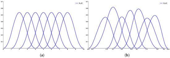
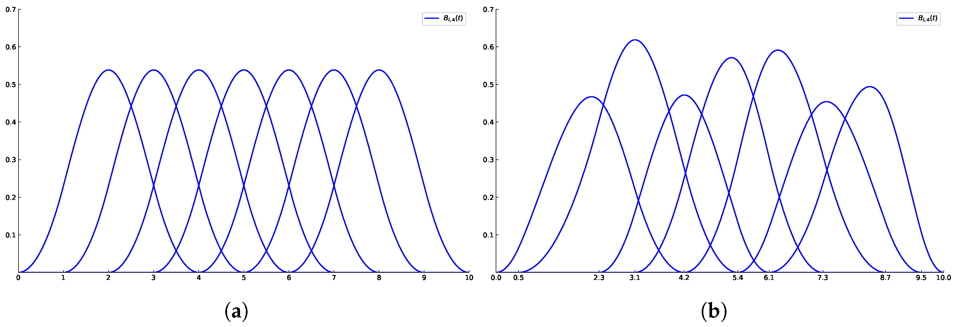
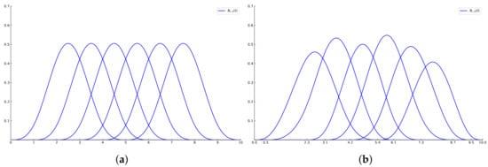
If $t_{j-1}<t_j=t_{j+1}=\dots =t_{j+l-1}<t_{j+l}$, then $t_j,t_{j+1},\dots ,t_{j+l-1}$ are referred to as knots of multiplicity l. Figure 1 illustrates the Ball-Spline basis functions of order 4. Under uniform knot spacing, the basis functions exhibit symmetric distributions.

Figure 1. Ball-Spline basis functions of order 4. (a) Uniform Ball-Spline basis functions; (b) non-uniform Ball-Spline basis functions.

Remark 1.

The parameters $A_i$ and $B_i$ are introduced to determine the coefficients of the piecewise polynomial segments in the Ball-Spline basis functions. They are obtained by imposing the normalization condition and the required continuity conditions at the knots. Moreover, under certain knot configurations with repeated knots, the resulting basis functions reduce to the classical cubic Ball basis functions. These requirements determine the expressions of $A_i$ and $B_i$ in Definition 1.

Remark 2.

$B_{i,4}\left(t\right)$, $A_i$, $B_i$ satisfy the following property:

If $f_i\left(t\right)=f(t;t_i,t_{i+1},\dots ,t_{i+k},\dots )$, then $f_{i+1}\left(t\right)=f(t;t_{i+1},t_{i+2},\dots ,t_{i+k+1},\dots )$.

2.2. Properties of Ball-Spline Basis Functions

In this subsection, we will give some basic properties of the functions $B_{i,4}\left(t\right)$.

Proposition 1

(Local Support Property). $B_{i,4}\left(t\right)=0$ for $t\notin [t_i,t_{i+4})$.

This property follows directly from the definition of the basis function.

Proposition 2

(Normalized Property). ${\displaystyle \sum _{j=-\infty }^{+\infty }}{B}_{j,4}\left(t\right)\equiv 1$ for $t\in [t_i,t_{i+1})$.

Proof. 

From Proposition 1, we have ${\displaystyle \sum _{j=-\infty }^{+\infty }}{B}_{i,4}\left(t\right)={\displaystyle \sum _{j=i-3}^i}{B}_{j,4}\left(t\right)$. From (1), together with the translation property in Remark 2, the four nonzero basis functions on the interval $[t_i,t_{i+1})$ can be obtained as follows:

$$\begin{array}{cc}\hfill B_{i-3,4}\left(t\right)=& 3B_{i-2}{\displaystyle \frac{t_{i+1}-t_i}{3t_{i+1}-t_i-2t_{i-1}}}{\left({\displaystyle \frac{t_{i+1}-t}{t_{i+1}-t_i}}\right)}^2\hfill \\ \hfill B_{i-2,4}\left(t\right)=& \left(6A_{i-1}{\displaystyle \frac{t_{i+1}-t_{i-1}}{2t_{i+1}+t_i-3t_{i-1}}}-2\right){\left({\displaystyle \frac{t_{i+1}-t}{t_{i+1}-t_i}}\right)}^3+3\left(1-B_{i-2}{\displaystyle \frac{t_{i+1}-t_i}{3t_{i+1}-t_i-2t_{i-1}}}-A_{i-1}\right){\left({\displaystyle \frac{t_{i+1}-t}{t_{i+1}-t_i}}\right)}^2\hfill \\ \hfill -& 6B_{i-1}{\displaystyle \frac{t_{i+2}-t_i}{3t_{i+2}-t_{i+1}-2t_i}}{\left({\displaystyle \frac{t-t_i}{t_{i+1}-t_i}}\right)}^3+3B_{i-1}{\left({\displaystyle \frac{t-t_i}{t_{i+1}-t_i}}\right)}^2\hfill \\ \hfill B_{i-1,4}\left(t\right)=& \left(6B_{i-1}{\displaystyle \frac{t_{i+2}-t_i}{3t_{i+2}-t_{i+1}-2t_i}}-2\right){\left({\displaystyle \frac{t-t_i}{t_{i+1}-t_i}}\right)}^3+3\left(1-B_{i-1}-A_i{\displaystyle \frac{t_{i+1}-t_i}{2t_{i+2}+t_{i+1}-3t_i}}\right){\left({\displaystyle \frac{t-t_i}{t_{i+1}-t_i}}\right)}^2\hfill \\ \hfill -& 6A_{i-1}{\displaystyle \frac{t_{i+1}-t_{i-1}}{2t_{i+1}+t_i-3t_{i-1}}}{\left({\displaystyle \frac{t_{i+1}-t}{t_{i+1}-t_i}}\right)}^3+3A_{i-1}{\left({\displaystyle \frac{t_{i+1}-t}{t_{i+1}-t_i}}\right)}^2\hfill \\ \hfill B_{i,4}\left(t\right)=& 3A_i{\displaystyle \frac{t_{i+1}-t_i}{2t_{i+2}+t_{i+1}-3t_i}}{\left({\displaystyle \frac{t-t_i}{t_{i+1}-t_i}}\right)}^2\hfill \end{array}$$

(3)

where $A_i$ and $B_i$ are given in (2). By mathematical derivation, we obtain, for $t\in [t_i,t_{i+1}),$

$$\begin{array}{cc}\hfill {\displaystyle \sum _{j=-\infty }^{+\infty }}{B}_{j,4}\left(t\right)& ={\displaystyle \sum _{j=i-3}^i}{B}_{j,4}\left(t\right)\hfill \\ \hfill & =B_{i-3,4}\left(t\right)+B_{i-2,4}\left(t\right)+B_{i-1,4}\left(t\right)+B_{i,4}\left(t\right)\hfill \\ \hfill & =3{\left({\displaystyle \frac{t-t_i}{t_{i+1}-t_i}}\right)}^2+3{\left({\displaystyle \frac{t_{i+1}-t}{t_{i+1}-t_i}}\right)}^2-2{\left({\displaystyle \frac{t-t_i}{t_{i+1}-t_i}}\right)}^3-2{\left({\displaystyle \frac{t_{i+1}-t}{t_{i+1}-t_i}}\right)}^3\hfill \end{array}$$

Let $\tau ={\displaystyle \frac{t-t_i}{t_{i+1}-t_i}}$, then $1-\tau ={\displaystyle \frac{t_{i+1}-t}{t_{i+1}-t_i}}$.

• Hence,

$$\begin{array}{cc}\hfill {\displaystyle \sum _{j=-\infty }^{+\infty }}{B}_{j,4}\left(t\right)& =3{\tau }^2+3{(1-\tau )}^2-2{\tau }^3-2{(1-\tau )}^3\hfill \\ & =3\left({\tau }^2+{(1-\tau )}^2\right)-2\left({\tau }^3+{(1-\tau )}^3\right)\hfill \\ & =3(1-2\tau +2{\tau }^2)-2(1-3\tau +3{\tau }^2)\hfill \\ & =1.\hfill \end{array}$$

□

Proposition 3

(Linear Independence).

(1) 

$B_{i-3,4}\left(t\right),B_{i-2,4}\left(t\right),B_{i-1,4}\left(t\right),B_{i,4}\left(t\right)$ are linearly independent on $[t_i,t_{i+1})$ for all i

(2) 

The functions ${\left\{B_{i,4}\left(t\right)\right\}}_{i=-\infty }^{+\infty }$ are linearly independent on $(-\infty ,+\infty )$.

Proof. 

We prove (1), and (2) follows easily from (1). Suppose ${\displaystyle \sum _{j=i-3}^i}{\alpha }_j{B}_{j,4}\left(t\right)=0$ for $t\in \left[t_i,t_{i+1}\right),$ i.e.,

$${\alpha }_{i-3}{B}_{i-3,4}\left(t\right)+{\alpha }_{i-2}{B}_{i-2,4}\left(t\right)+{\alpha }_{i-1}{B}_{i-1,4}\left(t\right)+{\alpha }_i{B}_{i,4}\left(t\right)=0.$$

From (3), through calculation and derivation, we obtain

$$\begin{array}{cc}\hfill & \left[3{\alpha }_{i-3}{B}_{i-2}{\displaystyle \frac{t_{i+1}-t_i}{3t_{i+1}-t_i-2t_{i-1}}}+3{\alpha }_{i-1}{A}_{i-1}+3{\alpha }_{i-2}\left(1-B_{i-2}{\displaystyle \frac{t_{i+1}-t_i}{3t_{i+1}-t_i-2t_{i-1}}}-A_{i-1}\right)\right]{\left({\displaystyle \frac{t_{i+1}-t}{t_{i+1}-t_i}}\right)}^2\hfill \\ \hfill & +\left[{\alpha }_{i-2}\left(6A_{i-1}{\displaystyle \frac{t_{i+1}-t_{i-1}}{2t_{i+1}+t_i-3t_{i-1}}}-2\right)-6{\alpha }_{i-1}{A}_{i-1}{\displaystyle \frac{t_{i+1}-t_{i-1}}{2t_{i+1}+t_i-3t_{i-1}}}\right]{\left({\displaystyle \frac{t_{i+1}-t}{t_{i+1}-t_i}}\right)}^3\hfill \\ \hfill & +\left[3{\alpha }_{i-2}{B}_{i-1}+3{\alpha }_i{A}_i{\displaystyle \frac{t_{i+1}-t_i}{2t_{i+2}+t_{i+1}-3t_i}}+3{\alpha }_{i-1}\left(1-B_{i-1}-A_i{\displaystyle \frac{t_{i+1}-t_i}{2t_{i+2}+t_{i+1}-3t_i}}\right)\right]{\left({\displaystyle \frac{t-t_i}{t_{i+1}-t_i}}\right)}^2\hfill \\ \hfill & +\left[-6{\alpha }_{i-2}{B}_{i-1}{\displaystyle \frac{t_{i+2}-t_i}{3t_{i+2}-t_{i+1}-2t_i}}+{\alpha }_{i-1}\left(6B_{i-1}{\displaystyle \frac{t_{i+2}-t_i}{3t_{i+2}-t_{i+1}-2t_i}}-2\right)\right]{\left({\displaystyle \frac{t-t_i}{t_{i+1}-t_i}}\right)}^3\hfill \\ \hfill & =0\hfill \end{array}$$

Because of the linear independence of

$${\left({\displaystyle \frac{t-t_i}{t_{i+1}-t_i}}\right)}^2,{\left({\displaystyle \frac{t-t_i}{t_{i+1}-t_i}}\right)}^3,{\left({\displaystyle \frac{t_{i+1}-t}{t_{i+1}-t_i}}\right)}^2,{\left({\displaystyle \frac{t_{i+1}-t}{t_{i+1}-t_i}}\right)}^3,$$

it follows that

$$\left\{\begin{array}{c}3{\alpha }_{i-3}{B}_{i-2}{\displaystyle \frac{t_{i+1}-t_i}{3t_{i+1}-t_i-2t_{i-1}}}+3{\alpha }_{i-2}\left(1-B_{i-2}{\displaystyle \frac{t_{i+1}-t_i}{3t_{i+1}-t_i-2t_{i-1}}}-A_{i-1}\right)+3{\alpha }_{i-1}{A}_{i-1}=0\hfill \\ {\alpha }_{i-2}\left(6A_{i-1}{\displaystyle \frac{t_{i+1}-t_{i-1}}{2t_{i+1}+t_i-3t_{i-1}}}-2\right)-6{\alpha }_{i-1}{A}_{i-1}{\displaystyle \frac{t_{i+1}-t_{i-1}}{2t_{i+1}+t_i-3t_{i-1}}}=0\hfill \\ 3{\alpha }_{i-2}{B}_{i-1}+3{\alpha }_{i-1}\left(1-B_{i-1}-A_i{\displaystyle \frac{t_{i+1}-t_i}{2t_{i+2}+t_{i+1}-3t_i}}\right)+3{\alpha }_i{A}_i{\displaystyle \frac{t_{i+1}-t_i}{2t_{i+2}+t_{i+1}-3t_i}}=0\hfill \\ -6{\alpha }_{i-2}{B}_{i-1}{\displaystyle \frac{t_{i+2}-t_i}{3t_{i+2}-t_{i+1}-2t_i}}+{\alpha }_{i-1}\left(6B_{i-1}{\displaystyle \frac{t_{i+2}-t_i}{3t_{i+2}-t_{i+1}-2t_i}}-2\right)=0\hfill \end{array}\right.$$

(4)

Treating ${\alpha }_{i-3},{\alpha }_{i-2},{\alpha }_{i-1},{\alpha }_i$ as unknowns, the coefficient matrix is denoted as $\mathit{D}$, then (4) is equivalent to $\mathit{D}\mathit{\alpha }=\mathit{O}$, where $\mathit{\alpha }={[{\alpha }_{i-3},{\alpha }_{i-2},{\alpha }_{i-1},{\alpha }_i]}^T$, $\mathit{O}={[0,0,0,0]}^T$ denotes the zero vector, and $\mathit{D}={\left(d_{ij}\right)}_{4\times 4},i,j=1,2,3,4.$ is given by

$$\begin{array}{cc}& d_{11}=3B_{i-2}{\displaystyle \frac{t_{i+1}-t_i}{3t_{i+1}-t_i-2t_{i-1}}},d_{12}=3\left(1-B_{i-2}{\displaystyle \frac{t_{i+1}-t_i}{3t_{i+1}-t_i-2t_{i-1}}}-A_{i-1}\right),d_{13}=3A_{i-1},\hfill \\ & d_{22}=6A_{i-1}{\displaystyle \frac{t_{i+1}-t_{i-1}}{2t_{i+1}+t_i-3t_{i-1}}}-2,d_{23}=-6A_{i-1}{\displaystyle \frac{t_{i+1}-t_{i-1}}{2t_{i+1}+t_i-3t_{i-1}}},d_{32}=3B_{i-1},\hfill \\ & d_{33}=3\left(1-B_{i-1}-A_i{\displaystyle \frac{t_{i+1}-t_i}{2t_{i+2}+t_{i+1}-3t_i}}\right),d_{34}=3A_i{\displaystyle \frac{t_{i+1}-t_i}{2t_{i+2}+t_{i+1}-3t_i}},\hfill \\ & d_{42}=-6B_{i-1}{\displaystyle \frac{t_{i+2}-t_i}{3t_{i+2}-t_{i+1}-2t_i}},d_{43}=6B_{i-1}{\displaystyle \frac{t_{i+2}-t_i}{3t_{i+2}-t_{i+1}-2t_i}}-2,\hfill \\ & d_{21}=d_{31}=d_{41}=d_{14}=d_{24}=d_{44}=0.\hfill \end{array}$$

Calculation shows that

$$\begin{array}{cc}\hfill \det & \mathit{D}=d_{11}{d}_{34}(d_{23}{d}_{42}-d_{22}{d}_{43})\hfill \\ & ={\displaystyle \frac{18A_i{B}_{i-2}{(t_{i+1}-t_i)}^2}{(3t_{i+1}-t_i-2t_{i-1})(2t_{i+2}+t_{i+1}-3t_i)}}\hfill \\ & ·\left(6A_{i-1}{\displaystyle \frac{t_{i+1}-t_{i-1}}{2t_{i+1}+t_i-3t_{i-1}}}+6B_{i-1}{\displaystyle \frac{t_{i+2}-t_i}{3t_{i+2}-t_{i+1}-2t_i}}-2\right)\hfill \end{array}$$

Set $h_i=t_{i+1}-t_i$. For $t\in [t_i,t_{i+1}),h_i>0$, from (2), we have

$$\begin{array}{cc}\hfill A_i& =1,B_{i-2}=1,\hfill \\ \hfill A_{i-1}& ={\displaystyle \frac{\left(2h_i+3h_{i-1}\right)h_{i-1}\left(2h_{i+1}+h_i\right)}{\left(h_{i-1}+h_i+h_{i+1}\right)\left(h_i^2+3h_{i-1}{h}_i+3h_i{h}_{i+1}+6h_{i-1}{h}_{i+1}\right)}}\hfill \\ \hfill B_{i-1}& ={\displaystyle \frac{\left(2h_i+3h_{i+1}\right)h_{i+1}\left(2h_{i-1}+h_i\right)}{\left(h_{i-1}+h_i+h_{i+1}\right)\left(h_i^2+3h_{i-1}{h}_i+3h_i{h}_{i+1}+6h_{i-1}{h}_{i+1}\right)}}\hfill \end{array}$$

Substituting into the above expression, we obtain

$$\det \mathit{D}=-{\displaystyle \frac{36h_i^4}{(2h_{i-1}+3h_i)(3h_i+2h_{i+1})\left(h_i^2+3h_{i-1}{h}_i+3h_i{h}_{i+1}+6h_{i-1}{h}_{i+1}\right)}}$$

Since $h_i>0$, $h_{i-1}\ge 0$, and $h_{i+1}\ge 0$, we have $2h_{i-1}+3h_i>0$, $3h_i+2h_{i+1}>0$, and $h_i^2+3h_{i-1}{h}_i+3h_i{h}_{i+1}+6h_{i-1}{h}_{i+1}>0$. Therefore, $\det \mathit{D}\ne 0$ and the homogeneous system $\mathit{D}\mathit{\alpha }=\mathit{O}$ has only the trivial solution ${\alpha }_{i-3}={\alpha }_{i-2}={\alpha }_{i-1}={\alpha }_i=0$. Hence, for all i, $B_{i-3,4}\left(t\right),B_{i-2,4}\left(t\right),B_{i-1,4}\left(t\right),B_{i,4}\left(t\right)$ are linearly independent on $[t_i,t_{i+1})$. □

Proposition 4

(Relation with cubic Ball basis functions). In the case $t_{i-3}=t_{i-2}=t_{i-1}=t_i<t_{i+1}=t_{i+2}=t_{i+3}=t_{i+4}$, $B_{i-3,4}\left(t\right),B_{i-2,4}\left(t\right),B_{i-1,4}\left(t\right),B_{i,4}\left(t\right)$ are just the cubic Ball basis functions: ${(1-\tau )}^2,2{(1-\tau )}^2\tau ,2(1-\tau ){\tau }^2,{\tau }^2$ on $[t_i,t_{i+1}]$, where $\tau ={\displaystyle \frac{t-t_i}{t_{i+1}-t_i}}$.

Proof. 

To simplify computations, we set $h_i=t_{i+1}-t_i$; then, $h_i\ge 0$. (2) is equivalent to the following expression:

$$\begin{array}{c}\hfill A_i=\left\{\begin{array}{c}0,h_i=h_{i+1}=0and{h}_{i+2}\ge 0,\hfill \\ 1,h_i>0and{h}_{i+1}=h_{i+2}=0,\hfill \\ {\displaystyle \frac{\left(2h_{i+1}+3h_i\right)h_i\left(2h_{i+2}+h_{i+1}\right)}{\left(h_i+h_{i+1}+h_{i+2}\right)\left(h_{i+1}^2+3h_i{h}_{i+1}+3h_{i+1}{h}_{i+2}+6h_i{h}_{i+2}\right)}},otherwise.\hfill \end{array}\right.\\ \hfill B_i=\left\{\begin{array}{c}1,h_i=h_{i+1}=0and{h}_{i+2}>0,\hfill \\ 0,h_i\ge 0and{h}_{i+1}=h_{i+2}=0,\hfill \\ {\displaystyle \frac{\left(2h_{i+1}+3h_{i+2}\right)h_{i+2}\left(2h_i+h_{i+1}\right)}{\left(h_i+h_{i+1}+h_{i+2}\right)\left(h_{i+1}^2+3h_i{h}_{i+1}+3h_{i+1}{h}_{i+2}+6h_i{h}_{i+2}\right)}},otherwise.\hfill \end{array}\right.\end{array}$$

(5)

When $t_{i-3}=t_{i-2}=t_{i-1}=t_i<t_{i+1}=t_{i+2}=t_{i+3}=t_{i+4}$, we have $h_{i-3}=h_{i-2}=h_{i-1}=0,h_i>0,h_{i+1}=h_{i+2}=h_{i+3}=0$. From (5) and translation properties,

$$\begin{array}{cc}\hfill A_i& =1,B_{i-2}=1,\hfill \\ \hfill A_{i-1}& ={\displaystyle \frac{\left(2h_i+3h_{i-1}\right)h_{i-1}\left(2h_{i+1}+h_i\right)}{\left(h_{i-1}+h_i+h_{i+1}\right)\left(h_i^2+3h_{i-1}{h}_i+3h_i{h}_{i+1}+6h_{i-1}{h}_{i+1}\right)}}\hfill \\ & ={\displaystyle \frac{h_{i-1}}{h_{i-1}+h_i+h_{i+1}}}\left[1+{\displaystyle \frac{h_i\left(h_i+h_{i+1}\right)}{h_i^2+3h_{i-1}{h}_i+3h_i{h}_{i+1}+6h_{i-1}{h}_{i+1}}}\right]=0,\hfill \\ \hfill B_{i-1}& ={\displaystyle \frac{\left(2h_i+3h_{i+1}\right)h_{i+1}\left(2h_{i-1}+h_i\right)}{\left(h_{i-1}+h_i+h_{i+1}\right)\left(h_i^2+3h_{i-1}{h}_i+3h_i{h}_{i+1}+6h_{i-1}{h}_{i+1}\right)}}\hfill \\ & ={\displaystyle \frac{h_{i+1}}{h_{i-1}+h_i+h_{i+1}}}\left[1+{\displaystyle \frac{h_i\left(h_i+h_{i-1}\right)}{h_i^2+3h_{i-1}{h}_i+3h_i{h}_{i+1}+6h_{i-1}{h}_{i+1}}}\right]=0.\hfill \end{array}$$

By substituting into (3), when $t_{i-3}=t_{i-2}=t_{i-1}=t_i<t_{i+1}=t_{i+2}=t_{i+3}=t_{i+4}$, we derive:

$$\begin{array}{cc}\hfill B_{i-3,4}\left(t\right)& ={\left({\displaystyle \frac{t_{i+1}-t}{t_{i+1}-t_i}}\right)}^2={(1-\tau )}^2\hfill \\ \hfill B_{i-2,4}\left(t\right)& =-2{\left({\displaystyle \frac{t_{i+1}-t}{t_{i+1}-t_i}}\right)}^3+2{\left({\displaystyle \frac{t_{i+1}-t}{t_{i+1}-t_i}}\right)}^2=2{\left({\displaystyle \frac{t_{i+1}-t}{t_{i+1}-t_i}}\right)}^2\left({\displaystyle \frac{t-t_i}{t_{i+1}-t_i}}\right)=2{(1-\tau )}^2\tau \hfill \\ \hfill B_{i-1,4}\left(t\right)& =-2{\left({\displaystyle \frac{t-t_i}{t_{i+1}-t_i}}\right)}^3+2{\left({\displaystyle \frac{t-t_i}{t_{i+1}-t_i}}\right)}^2=2\left({\displaystyle \frac{t_{i+1}-t}{t_{i+1}-t_i}}\right){\left({\displaystyle \frac{t-t_i}{t_{i+1}-t_i}}\right)}^2=2(1-\tau ){\tau }^2\hfill \\ \hfill B_{i,4}\left(t\right)& ={\left({\displaystyle \frac{t-t_i}{t_{i+1}-t_i}}\right)}^2={\tau }^2\hfill \end{array}$$

Therefore, in the case $t_{i-3}=t_{i-2}=t_{i-1}=t_i<t_{i+1}=t_{i+2}=t_{i+3}=t_{i+4}$, $B_{i-3,4}\left(t\right),B_{i-2,4}\left(t\right),B_{i-1,4}\left(t\right),B_{i,4}\left(t\right)$ can degenerate into the cubic Ball basis functions on $[t_i,t_{i+1}]$, i.e., the degeneracy property holds. □

In addition, we note that the proposed Ball-Spline basis is constructed differently from parametric generalized Ball-type bases, such as the $\lambda \mu$–Ball basis [38] and the QGS–Ball basis [39]. However, they share a similar degeneracy behavior under special parameter choices. For the $\lambda \mu$–Ball basis, when $\lambda =\mu =0$, it reduces to the classical cubic Ball basis. For the QGS–Ball basis, when ${\lambda }_1={\lambda }_2={\lambda }_3=0$, it reduces to the classical Said–Ball basis, and when ${\lambda }_1={\lambda }_3=0,{\lambda }_2=-3$, it further reduces to the cubic Bernstein basis.

This shows that different generalized Ball-type bases have different degeneracy paths. The proposed Ball-Spline basis is formulated within the spline framework and relies on knot multiplicity rather than shape parameters.

Lemma 1.

The basis function $B_{i,4}\left(t\right)$ defined in (1) can be expressed as a linear combination of changeable-degree spline basis functions (CD-spline basis) [9], i.e.,

$$B_{i,4}\left(t\right)=\overline{A_i}{N}_{i,4}\left(t\right)+\overline{B_i}{N}_{i+1,4}\left(t\right)+\overline{C_i}{N}_{i+2,4}\left(t\right)$$

(6)

where $N_{i,4}\left(t\right),N_{i+1,4}\left(t\right),N_{i+2,4}\left(t\right)$ are changeable-degree spline basis functions given by:

$$\begin{array}{c}{N}_{i,4}\left(t\right)=\left\{\begin{array}{c}{\displaystyle \frac{3{\left(t-t_i\right)}^2}{\left(t_{i+1}-t_i\right)\left(t_{i+1}+2t_{i+2}-3t_i\right)}},t\in [t_i,t_{i+1})\hfill \\ {\displaystyle \frac{-3t+t_{i+1}+t_{i+2}+t_{i+3}}{t_{i+3}-t_{i+1}}}-{\displaystyle \frac{2{\left(t_{i+2}-t\right)}^3}{{(t_{i+2}-t_{i+1})}^2\left(t_{i+1}+2t_{i+2}-3t_i\right)}}\hfill \\ -{\displaystyle \frac{{\left(t_{i+2}-t\right)}^3}{\left(t_{i+3}-t_{i+1}\right){\left(t_{i+2}-t_{i+1}\right)}^2}}+{\displaystyle \frac{{\left(t-t_{i+1}\right)}^3}{(t_{i+2}-t_{i+1}){\left(t_{i+3}-t_{i+1}\right)}^2}},t\in [t_{i+1},t_{i+2})\hfill \\ {\displaystyle \frac{{\left(t_{i+3}-t\right)}^3}{\left(t_{i+3}-t_{i+2}\right){\left(t_{i+3}-t_{i+1}\right)}^2}},t\in [t_{i+2},t_{i+3})\hfill \end{array}\right.\hfill \end{array}$$

(7)

$$\begin{array}{c}{N}_{i+1,4}\left(t\right)=\left\{\begin{array}{c}{\displaystyle \frac{3t-2t_{i+1}-t_{i+2}}{t_{i+3}-t_{i+1}}}+{\displaystyle \frac{{\left(t_{i+2}-t\right)}^3}{{\left(t_{i+2}-t_{i+1}\right)}^2\left(t_{i+3}-t_{i+1}\right)}}-{\displaystyle \frac{2{\left(t-t_{i+1}\right)}^3}{\left(t_{i+2}-t_{i+1}\right){\left(t_{i+3}-t_{i+1}\right)}^2}},t\in [t_{i+1},t_{i+2})\hfill \\ {\displaystyle \frac{t_{i+2}+2t_{i+3}-3t}{t_{i+3}-t_{i+1}}}+{\displaystyle \frac{{\left(t-t_{i+2}\right)}^3}{{\left(t_{i+3}-t_{i+2}\right)}^2\left(t_{i+3}-t_{i+1}\right)}}-{\displaystyle \frac{2{\left(t_{i+3}-t\right)}^3}{\left(t_{i+3}-t_{i+2}\right){\left(t_{i+3}-t_{i+1}\right)}^2}},t\in [t_{i+2},t_{i+3})\hfill \end{array}\right.\hfill \end{array}$$

(8)

$$\begin{array}{c}{N}_{i+2,4}\left(t\right)=\left\{\begin{array}{c}{\displaystyle \frac{{(t-t_{i+1})}^3}{\left(t_{i+2}-t_{i+1}\right){\left(t_{i+3}-t_{i+1}\right)}^2}},t\in [t_{i+1},t_{i+2})\hfill \\ {\displaystyle \frac{3t-t_{i+1}-t_{i+2}-t_{i+3}}{t_{i+3}-t_{i+1}}}-{\displaystyle \frac{2{\left(t-t_{i+2}\right)}^3}{{\left(t_{i+3}-t_{i+2}\right)}^2\left(3t_{i+4}-t_{i+3}-2t_{i+2}\right)}}\hfill \\ -{\displaystyle \frac{{\left(t-t_{i+2}\right)}^3}{{\left(t_{i+3}-t_{i+2}\right)}^2\left(t_{i+3}-t_{i+1}\right)}}+{\displaystyle \frac{{\left(t_{i+3}-t\right)}^3}{\left(t_{i+3}-t_{i+2}\right){\left(t_{i+3}-t_{i+1}\right)}^2}},t\in [t_{i+2},t_{i+3})\hfill \\ {\displaystyle \frac{3{\left(t_{i+4}-t\right)}^2}{\left(t_{i+4}-t_{i+3}\right)\left(3t_{i+4}-t_{i+3}-2t_{i+2}\right)}},t\in [t_{i+3},t_{i+4})\hfill \end{array}\right.\hfill \end{array}$$

(9)

and the coefficient $\overline{A_i},\overline{B_i},\overline{C_i}$ are given by

$$\begin{array}{c}\overline{A_i}=A_i,\overline{C_i}=B_{i+1},\hfill \\ \overline{B_i}=\left\{\begin{array}{c}{\displaystyle \frac{2}{3}},t_i<t_{i+1}=t_{i+2}=t_{i+3}<t_{i+4},t_i=t_{i+1}=t_{i+2}\le t_{i+3}<t_{i+4}\hfill \\ or{t}_i<t_{i+1}\le t_{i+2}=t_{i+3}=t_{i+4},\hfill \\ {\displaystyle \frac{t_{i+3}-t_{i+1}}{t_{i+3}-t_{i+2}}}\left[1-A_{i+1}-B_{i+1}{\displaystyle \frac{t_{i+2}-t_{i+1}}{t_{i+3}-t_{i+1}}}-B_i{\displaystyle \frac{t_{i+3}-t_{i+2}}{3t_{i+3}-t_{i+2}-2t_{i+1}}}\right],otherwise.\hfill \end{array}\right.\hfill \end{array}$$

(10)

The coefficients $\overline{A_i}$, $\overline{B_i}$, and $\overline{C_i}$ are determined by comparing the Ball-Spline basis function with its CD-spline representation in (6). Specifically, (1) is equated with (6), and the coefficients of the corresponding piecewise polynomial segments on each knot subinterval are matched. In this way, $\overline{A_i}=A_i$ and $\overline{C_i}=B_{i+1}$ are obtained directly, while $\overline{B_i}$ is determined from the remaining middle segment. Moreover, to preserve the same degeneracy behavior as (1) under the corresponding multiple-knot configurations, $\overline{B_i}$ reduces to $2/3$ in these cases. A more detailed derivation is given in the following proof.

Proof. 

Here, we will prove that Equation (1) is equivalent to Equation (6), and the equivalence can be proven through the transition using the following expression. From (6), it can be calculated that

$$\begin{array}{c}\hfill \begin{array}{c}{B}_{i,4}\left(t\right)=\left\{\begin{array}{c}3\overline{A_i}{\displaystyle \frac{t_{i+1}-t_i}{2t_{i+2}+t_{i+1}-3t_i}}{\left({\displaystyle \frac{t-t_i}{t_{i+1}-t_i}}\right)}^2,t\in [t_i,t_{i+1})\hfill \\ [\overline{C_i}{\left({\displaystyle \frac{t_{i+2}-t_{i+1}}{t_{i+3}-t_{i+1}}}\right)}^2-\overline{A_i}{\displaystyle \frac{\left(t_{i+3}-t_{i+2}\right)\left(2t_{i+3}+t_{i+2}-3t_{i+1}\right)}{{\left(t_{i+3}-t_{i+1}\right)}^2}}\hfill \\ -\overline{B_i}{\displaystyle \frac{\left(t_{i+2}-t_{i+1}\right)\left(t_{i+3}+2t_{i+2}-3t_{i+1}\right)}{{\left(t_{i+3}-t_{i+1}\right)}^2}}]{\left({\displaystyle \frac{t-t_{i+1}}{t_{i+2}-t_{i+1}}}\right)}^3+3\left[\overline{B_i}{\displaystyle \frac{t_{i+2}-t_{i+1}}{t_{i+3}-t_{i+1}}}+\overline{A_i}{\displaystyle \frac{t_{i+3}-t_{i+2}}{t_{i+3}-t_{i+1}}}\right]{\left({\displaystyle \frac{t-t_{i+1}}{t_{i+2}-t_{i+1}}}\right)}^2\hfill \\ -6\overline{A_i}{\displaystyle \frac{t_{i+2}-t_i}{2t_{i+2}+t_{i+1}-3t_i}}{\left({\displaystyle \frac{t_{i+2}-t}{t_{i+2}-t_{i+1}}}\right)}^3+3\overline{A_i}{\left({\displaystyle \frac{t_{i+2}-t}{t_{i+2}-t_{i+1}}}\right)}^2,t\in [t_{i+1},t_{i+2})\hfill \\ [\overline{A_i}{\left({\displaystyle \frac{t_{i+3}-t_{i+2}}{t_{i+3}-t_{i+1}}}\right)}^2-\overline{C_i}{\displaystyle \frac{\left(t_{i+2}-t_{i+1}\right)\left(3t_{i+3}-t_{i+2}-2t_{i+1}\right)}{{\left(t_{i+3}-t_{i+1}\right)}^2}}\hfill \\ -\overline{B_i}{\displaystyle \frac{\left(t_{i+3}-t_{i+2}\right)\left(3t_{i+3}-2t_{i+2}-t_{i+1}\right)}{{\left(t_{i+3}-t_{i+1}\right)}^2}}]{\left({\displaystyle \frac{t_{i+3}-t}{t_{i+3}-t_{i+2}}}\right)}^3+3\left[\overline{B_i}{\displaystyle \frac{t_{i+3}-t_{i+2}}{t_{i+3}-t_{i+1}}}+\overline{C_i}{\displaystyle \frac{t_{i+2}-t_{i+1}}{t_{i+3}-t_{i+2}}}\right]{\left({\displaystyle \frac{t_{i+3}-t}{t_{i+3}-t_{i+2}}}\right)}^2\hfill \\ -6\overline{C_i}{\displaystyle \frac{t_{i+4}-t_{i+2}}{3t_{i+4}-t_{i+3}-2t_{i+2}}}{\left({\displaystyle \frac{t-t_{i+2}}{t_{i+3}-t_{i+2}}}\right)}^3+3\overline{C_i}{\left({\displaystyle \frac{t-t_{i+2}}{t_{i+3}-t_{i+2}}}\right)}^2,t\in [t_{i+2},t_{i+3})\hfill \\ 3\overline{C_i}{\displaystyle \frac{t_{i+4}-t_{i+3}}{3t_{i+4}-t_{i+3}-2t_{i+2}}}{\left({\displaystyle \frac{t_{i+4}-t}{t_{i+4}-t_{i+3}}}\right)}^2,t\in [t_{i+3},t_{i+4})\hfill \end{array}\right.\hfill \end{array}\end{array}$$

(11)

By substituting (10) into (11), we verify the equivalence piecewise. For $t\in [t_i,t_{i+1})$, since ${\overline{A}}_i=A_i$, the first branch of (11) becomes

$$3A_i{\displaystyle \frac{t_{i+1}-t_i}{2t_{i+2}+t_{i+1}-3t_i}}{\left({\displaystyle \frac{t-t_i}{t_{i+1}-t_i}}\right)}^2,$$

which coincides with the first branch of (1). For $t\in [t_{i+1},t_{i+2})$, substituting ${\overline{A}}_i=A_i$, ${\overline{C}}_i=B_{i+1}$, and ${\overline{B}}_i$ from (10) into the second branch of (11), we obtain

$$\begin{array}{cc}\hfill B_{i,4}\left(t\right)=& [B_{i+1}{\left({\displaystyle \frac{t_{i+2}-t_{i+1}}{t_{i+3}-t_{i+1}}}\right)}^2-A_i{\displaystyle \frac{(t_{i+3}-t_{i+2})(2t_{i+3}+t_{i+2}-3t_{i+1})}{{(t_{i+3}-t_{i+1})}^2}}\hfill \\ & -{\overline{B}}_i{\displaystyle \frac{(t_{i+2}-t_{i+1})(t_{i+3}+2t_{i+2}-3t_{i+1})}{{(t_{i+3}-t_{i+1})}^2}}]{\left({\displaystyle \frac{t-t_{i+1}}{t_{i+2}-t_{i+1}}}\right)}^3\hfill \\ & +3\left[{\overline{B}}_i{\displaystyle \frac{t_{i+2}-t_{i+1}}{t_{i+3}-t_{i+1}}}+A_i{\displaystyle \frac{t_{i+3}-t_{i+2}}{t_{i+3}-t_{i+1}}}\right]{\left({\displaystyle \frac{t-t_{i+1}}{t_{i+2}-t_{i+1}}}\right)}^2\hfill \\ & -6A_i{\displaystyle \frac{t_{i+2}-t_i}{2t_{i+2}+t_{i+1}-3t_i}}{\left({\displaystyle \frac{t_{i+2}-t}{t_{i+2}-t_{i+1}}}\right)}^3+3A_i{\left({\displaystyle \frac{t_{i+2}-t}{t_{i+2}-t_{i+1}}}\right)}^2.\hfill \end{array}$$

By the definition of ${\overline{B}}_i$ in (10), and by substituting (2), the coefficient of ${\left({\displaystyle \frac{t-t_{i+1}}{t_{i+2}-t_{i+1}}}\right)}^2$ satisfies

$$3\left[{\overline{B}}_i{\displaystyle \frac{t_{i+2}-t_{i+1}}{t_{i+3}-t_{i+1}}}+A_i{\displaystyle \frac{t_{i+3}-t_{i+2}}{t_{i+3}-t_{i+1}}}\right]=3\left(1-B_i-A_{i+1}{\displaystyle \frac{t_{i+2}-t_{i+1}}{2t_{i+3}+t_{i+2}-3t_{i+1}}}\right),$$

and the coefficient of ${\left({\displaystyle \frac{t-t_{i+1}}{t_{i+2}-t_{i+1}}}\right)}^3$ satisfies

$$\begin{array}{cc}& B_{i+1}{\left({\displaystyle \frac{t_{i+2}-t_{i+1}}{t_{i+3}-t_{i+1}}}\right)}^2-A_i{\displaystyle \frac{(t_{i+3}-t_{i+2})(2t_{i+3}+t_{i+2}-3t_{i+1})}{{(t_{i+3}-t_{i+1})}^2}}\hfill \\ & -{\overline{B}}_i{\displaystyle \frac{(t_{i+2}-t_{i+1})(t_{i+3}+2t_{i+2}-3t_{i+1})}{{(t_{i+3}-t_{i+1})}^2}}=6B_i{\displaystyle \frac{t_{i+3}-t_{i+1}}{3t_{i+3}-t_{i+2}-2t_{i+1}}}-2.\hfill \end{array}$$

Hence the second branch of (11) reduces to the second branch of (1). The same reasoning and direct calculations apply to $t\in [t_{i+2},t_{i+3})$ and $t\in [t_{i+3},t_{i+4})$, yielding the corresponding branches of (1).

Therefore, (11) is equivalent to (1). Hence (6) and (1) are equivalent. □

Remark 3.

From Lemma 1, each Ball-Spline basis function $B_{i,4}\left(t\right)$ can be represented as a linear combination of three CD-spline basis functions:

$$B_{i,4}\left(t\right)=\overline{A_i}{N}_{i,4}\left(t\right)+\overline{B_i}{N}_{i+1,4}\left(t\right)+\overline{C_i}{N}_{i+2,4}\left(t\right).$$

Although the Ball-Spline basis functions satisfy the translation property stated in Remark 2, the property does not carry over to their representations in terms of CD-spline basis functions.

In fact, the translated basis function $B_{i+1,4}\left(t\right)$ must be expressed using a different set of CD-spline basis functions and can be written as

$$B_{i+1,4}\left(t\right)=\overline{A_{i+1}}{M}_{i+1,4}\left(t\right)+\overline{B_{i+1}}{M}_{i+2,4}\left(t\right)+\overline{C_{i+1}}{M}_{i+3,4}\left(t\right),$$

where $M_{i+1,4}\left(t\right),M_{i+2,4}\left(t\right),M_{i+3,4}\left(t\right)$ are defined on a shifted knot sequence. It should be noted that CD-spline basis functions do not possess the translation property, because their local polynomial degrees are determined by a prescribed local degree vector and cannot be shifted consistently with the knot sequence. Consequently, the spline space spanned by the CD-spline basis depends on the specified local degree vector and $N_{i,4}\left(t\right),N_{i+1,4}\left(t\right),N_{i+2,4}\left(t\right)$ and $M_{i+1,4}\left(t\right),M_{i+2,4}\left(t\right),M_{i+3,4}\left(t\right)$ generally belong to different CD-spline spaces.

Remark 4.

The Ball-Spline basis functions we constructed are different from CD-spline basis functions. To further clarify the difference, we consider the spline space associated with the Ball-Spline basis. We consider

$${\Omega }_4\left(T\right):=\left\{f\left(t\right)|f\left(t\right){|}_{[t_j,t_{j+1})}\in {\mathbb{P}}_3,f^{\left(m\right)}\left(t_j^{-}\right)=f^{\left(m\right)}\left(t_j^{+}\right),m \mathit{determined} \mathit{by} \mathit{Proposition} \mathsf{6}\right\},$$

where ${\mathbb{P}}_3$ denotes the space of polynomials of degree at most 3. The Ball-Spline basis functions $B_{i,4}\left(t\right)$ form a basis of the space ${\Omega }_4\left(T\right)$.

In contrast, CD-spline basis functions are defined over a different spline space. Let $\mathit{U}={\left\{u_j\right\}}_{j=-\infty }^{+\infty }$ be a nondecreasing knot sequence, i.e., $u_j\le u_{j+1}$ for all $j\in \mathbb{Z}$, and let $\mathit{d}={\left\{d_j\right\}}_{j\in \mathbb{Z}}$ be a prescribed degree vector. If $u_{j-1}<u_j=u_{j+1}=\dots =u_{j+l-1}<u_{j+l}$, then $u_j,u_{j+1},\dots ,u_{j+l-1}$ are referred to as knots of multiplicity l. The associated CD-spline space is defined as

$$\mathcal{S}(U,\mathit{d}):=\left\{f\left(t\right)|f\left(t\right){|}_{[u_j,u_{j+1})}\in {\mathbb{P}}_{d_j},f^{\left(k\right)}\left(u_j^{-}\right)=f^{\left(k\right)}\left(u_j^{+}\right),0\le k\le r_j\right\},$$

where the continuity order $r_j$ satisfies

$$r_j\le \min \{d_{j-1},d_j\}-l,$$

and l denotes the multiplicity of the knot $u_j$. Here, ${\mathbb{P}}_{d_j}$ denotes the space of polynomials of degree at most $d_j$ on the interval $[u_j,u_{j+1})$.

From the above definitions, ${\Omega }_4\left(T\right)$ is a cubic spline space with degree variation restricted to the interior of individual basis functions, while the CD-spline space $S(U,d)$ allows polynomial degrees to vary explicitly from one interval to another. An example is given below to clarify this.

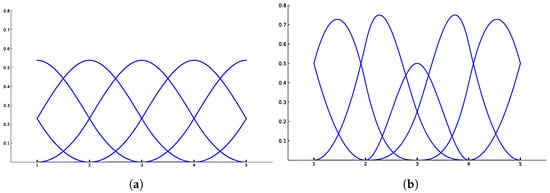
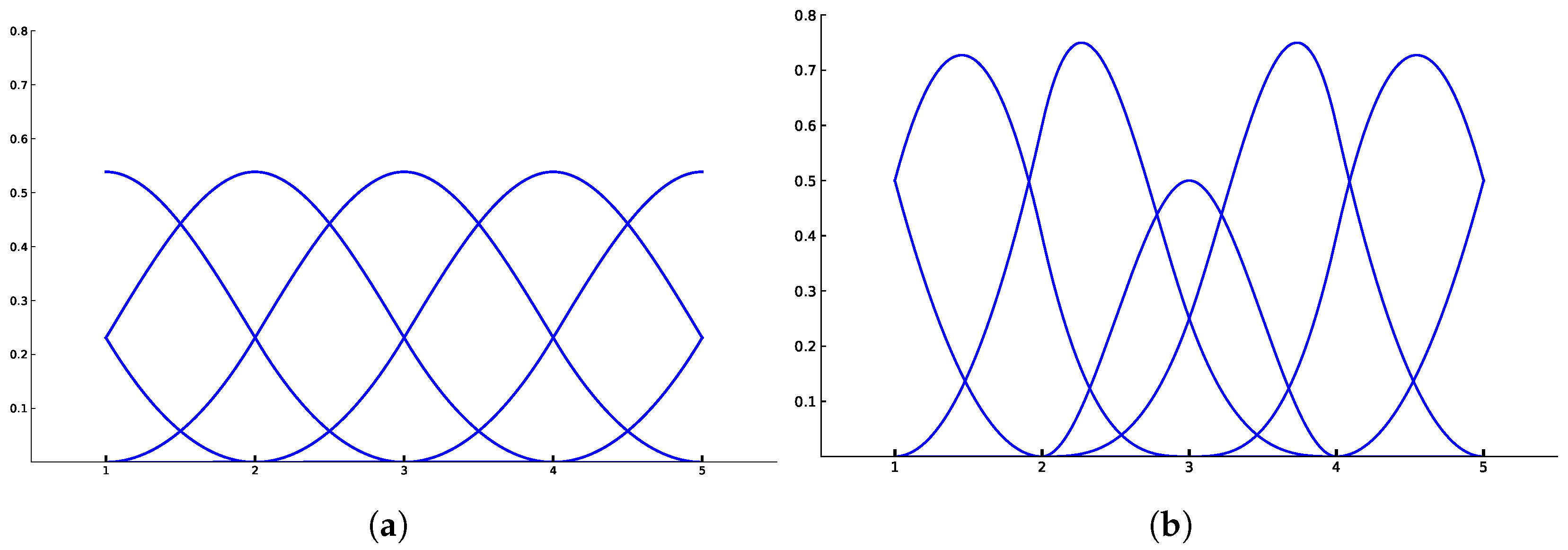
Figure 2 illustrates the distribution of 4th-order basis functions over four consecutive intervals: as shown in Figure 2a, the Ball-Spline basis consistently maintains four non-zero basis functions across all intervals. Its innovative 2, 3, 3, 2 degree structure is achieved by varying the degrees of individual polynomial segments within each basis function, without altering the overall dimensionality of the basis function space. Thus, the space it spans remains a cubic spline space. In contrast, in Figure 2b, the number and degrees of non-zero CD-spline basis functions depend on its degree vector and knot vector with

$$\mathit{d}=\{\dots ,2,3,3,2,\dots \},$$

i.e., in a degree-2 interval, only three non-zero quadratic basis functions exist, while in a degree-3 interval, four non-zero cubic basis functions exist. This indicates that the dimensionality of the space spanned by CD-spline basis functions changes dynamically.

Figure 2. Distribution of Ball-Spline and CD-spline basis functions of order 4. (a) Ball-Spline basis functions; (b) CD-spline basis functions.

Proposition 5

(Positivity Property). $B_{i,4}\left(t\right)>0$ for $t\in (t_i,t_{i+4})$

Proof. 

We prove this property based on the above lemma 1. Here we prove that the basis functions expressed by (6) are positive on $(t_i,t_{i+4})$. According to the positivity property of the CD-spline basis functions, $N_{i,4}\left(t\right),N_{i+1,4}\left(t\right),N_{i+2,4}\left(t\right)$ are positive on their corresponding support interval. We discuss the signs of $\overline{A_i},\overline{B_i},and\overline{C_i}$ separately in the following cases.

Set $h_i=t_{i+1}-t_i$, then $h_i\ge 0$.

(i)

In the case of single knot.

When $t_i<t_{i+1}<t_{i+2}<t_{i+3}<t_{i+4}$, here $h_i,h_{i+1},h_{i+2},h_{i+3}>0.$ From (10) and mathematical derivation, we have

$$\begin{array}{cc}& \overline{A_i}={\displaystyle \frac{h_i}{h_i+h_{i+1}+h_{i+2}}}\left[1+{\displaystyle \frac{h_{i+1}\left(h_{i+1}+h_{i+2}\right)}{h_{i+1}^2+3h_{i+1}{h}_{i+2}+3h_i{h}_{i+1}+6h_i{h}_{i+2}}}\right]>0,\hfill \\ & \overline{C_i}={\displaystyle \frac{h_{i+3}}{h_{i+1}+h_{i+2}+h_{i+3}}}\left[1+{\displaystyle \frac{h_{i+2}\left(h_{i+2}+h_{i+1}\right)}{h_{i+2}^2+3h_{i+2}{h}_{i+3}+3h_{i+1}{h}_{i+2}+6h_{i+1}{h}_{i+3}}}\right]>0.\hfill \end{array}$$

$$\begin{array}{cc}\hfill \overline{B_i}& =1-{\displaystyle \frac{h_{i+1}+h_{i+2}}{h_{i+1}+h_{i+2}+h_{i+3}}}·{\displaystyle \frac{h_{i+1}\left(h_{i+2}+h_{i+3}\right)}{3h_{i+1}\left(h_{i+2}+2h_{i+3}\right)+h_{i+2}\left(h_{i+2}+2h_{i+3}\right)}}\hfill \\ \hfill & -{\displaystyle \frac{h_{i+1}}{h_{i+1}+h_{i+2}+h_{i+3}}}·{\displaystyle \frac{h_{i+3}\left(h_{i+1}+h_{i+2}\right)}{3h_{i+3}\left(2h_{i+1}+h_{i+2}\right)+h_{i+2}\left(h_{i+2}+3h_{i+1}\right)}}\hfill \\ \hfill & -{\displaystyle \frac{h_{i+1}+h_{i+2}}{h_i+h_{i+1}+h_{i+2}}}·{\displaystyle \frac{h_{i+2}\left(2h_i+h_{i+1}\right)}{3h_{i+2}\left(2h_i+h_{i+1}\right)+h_{i+1}\left(h_{i+1}+3h_i\right)}}.\hfill \end{array}$$

(12)

Since $h_j>0$ for $j=i,i+1,i+2,i+3$, we have

$$0<{\displaystyle \frac{h_{i+1}+h_{i+2}}{h_{i+1}+h_{i+2}+h_{i+3}}}<1,0<{\displaystyle \frac{h_{i+1}}{h_{i+1}+h_{i+2}+h_{i+3}}}<1,$$

and

$$0<{\displaystyle \frac{h_{i+1}+h_{i+2}}{h_i+h_{i+1}+h_{i+2}}}<1.$$

Moreover,

$$3h_{i+1}(h_{i+2}+2h_{i+3})+h_{i+2}(h_{i+2}+2h_{i+3})>3h_{i+1}(h_{i+2}+2h_{i+3}),$$

$$3h_{i+3}(2h_{i+1}+h_{i+2})+h_{i+2}(h_{i+2}+3h_{i+1})>3h_{i+3}(2h_{i+1}+h_{i+2}),$$

and

$$3h_{i+2}(2h_i+h_{i+1})+h_{i+1}(h_{i+1}+3h_i)>3h_{i+2}(2h_i+h_{i+1}).$$

Hence,

$$\begin{array}{cc}\hfill \overline{B_i}& >1-{\displaystyle \frac{h_{i+1}(h_{i+2}+h_{i+3})}{3h_{i+1}(h_{i+2}+2h_{i+3})}}-{\displaystyle \frac{h_{i+3}(h_{i+1}+h_{i+2})}{3h_{i+3}(2h_{i+1}+h_{i+2})}}-{\displaystyle \frac{h_{i+2}(2h_i+h_{i+1})}{3h_{i+2}(2h_i+h_{i+1})}}.\hfill \end{array}$$

Furthermore,

$${\displaystyle \frac{h_{i+1}(h_{i+2}+h_{i+3})}{3h_{i+1}(h_{i+2}+2h_{i+3})}}={\displaystyle \frac{h_{i+2}+h_{i+3}}{3(h_{i+2}+2h_{i+3})}}<{\displaystyle \frac{h_{i+2}+2h_{i+3}}{3(h_{i+2}+2h_{i+3})}}={\displaystyle \frac{1}{3}},$$

$${\displaystyle \frac{h_{i+3}(h_{i+1}+h_{i+2})}{3h_{i+3}(2h_{i+1}+h_{i+2})}}={\displaystyle \frac{h_{i+1}+h_{i+2}}{3(2h_{i+1}+h_{i+2})}}<{\displaystyle \frac{2h_{i+1}+h_{i+2}}{3(2h_{i+1}+h_{i+2})}}={\displaystyle \frac{1}{3}},$$

and

$${\displaystyle \frac{h_{i+2}(2h_i+h_{i+1})}{3h_{i+2}(2h_i+h_{i+1})}}={\displaystyle \frac{1}{3}}.$$

Therefore,

$$\overline{B_i}>1-{\displaystyle \frac{1}{3}}-{\displaystyle \frac{1}{3}}-{\displaystyle \frac{1}{3}}=0.$$

Therefore, in the case of simple knot sequence, $\overline{A_i},\overline{B_i},\overline{C_i}>0$. Combining with the positivity property of the changeable-degree spline basis functions, the basis function $B_{i,4}\left(t\right)>0$ for $t\in (t_i,t_{i+4})$ holds.

(ii)

In the case of knots of multiplicity 2.

When $t_i=t_{i+1}<t_{i+2}<t_{i+3}<t_{i+4}$, here $h_i=0,h_{i+1},h_{i+2},h_{i+3}>0.$ From (10) and mathematical derivation, we have

$$\begin{array}{cc}& \overline{A_i}={\displaystyle \frac{h_i}{h_i+h_{i+1}+h_{i+2}}}\left[1+{\displaystyle \frac{h_{i+1}\left(h_{i+1}+h_{i+2}\right)}{h_{i+1}^2+3h_{i+1}{h}_{i+2}+3h_i{h}_{i+1}+6h_i{h}_{i+2}}}\right]=0,\hfill \\ & \overline{C_i}={\displaystyle \frac{h_{i+3}}{h_{i+1}+h_{i+2}+h_{i+3}}}\left[1+{\displaystyle \frac{h_{i+2}\left(h_{i+2}+h_{i+1}\right)}{h_{i+2}^2+3h_{i+2}{h}_{i+3}+3h_{i+1}{h}_{i+2}+6h_{i+1}{h}_{i+3}}}\right]>0,\hfill \end{array}$$

$$\begin{array}{cc}\hfill \overline{B_i}& =1-{\displaystyle \frac{\left(h_{i+1}+h_{i+2}\right)}{\left(h_{i+1}+h_{i+2}+h_{i+3}\right)}}·{\displaystyle \frac{h_{i+1}\left(h_{i+2}+h_{i+3}\right)}{3h_{i+1}\left(h_{i+2}+2h_{i+3}\right)+h_{i+2}\left(h_{i+2}+2h_{i+3}\right)}}\hfill \\ & -{\displaystyle \frac{h_{i+1}}{\left(h_{i+1}+h_{i+2}+h_{i+3}\right)}}·{\displaystyle \frac{h_{i+3}\left(h_{i+1}+h_{i+2}\right)}{3h_{i+3}\left(2h_{i+1}+h_{i+2}\right)+h_{i+2}\left(h_{i+2}+3h_{i+1}\right)}}-{\displaystyle \frac{h_{i+2}}{3h_{i+2}+h_{i+1}}}\hfill \end{array}$$

Similarly,

$$\begin{array}{cc}\hfill \overline{B_i}& >1-{\displaystyle \frac{h_{i+1}\left(h_{i+2}+h_{i+3}\right)}{3h_{i+1}\left(h_{i+2}+2h_{i+3}\right)}}-{\displaystyle \frac{h_{i+3}\left(h_{i+1}+h_{i+2}\right)}{3h_{i+3}\left(2h_{i+1}+h_{i+2}\right)}}-{\displaystyle \frac{h_{i+2}}{3h_{i+2}+h_{i+1}}}\hfill \\ & >1-{\displaystyle \frac{h_{i+2}+h_{i+3}}{3\left(h_{i+2}+2h_{i+3}\right)}}-{\displaystyle \frac{h_{i+1}+h_{i+2}}{3\left(2h_{i+1}+h_{i+2}\right)}}-{\displaystyle \frac{1}{3}}\hfill \\ & >1-{\displaystyle \frac{1}{3}}-{\displaystyle \frac{1}{3}}-{\displaystyle \frac{1}{3}}=0.\hfill \end{array}$$

When $t_i<t_{i+1}=t_{i+2}<t_{i+3}<t_{i+4}$, here $h_i>0,h_{i+1}=0,h_{i+2},h_{i+3}>0.$ From (10) and mathematical derivation, we have

$$\begin{array}{cc}& \overline{A_i}={\displaystyle \frac{h_i}{h_i+h_{i+2}}}>0,\overline{C_i}={\displaystyle \frac{h_{i+3}}{h_{i+2}+h_{i+3}}}\left[1+{\displaystyle \frac{h_{i+2}^2}{h_{i+2}^2+3h_{i+2}{h}_{i+3}}}\right]>0,\hfill \\ & \overline{B_i}=1-{\displaystyle \frac{h_{i+2}}{3(h_i+h_{i+2})}}>1-{\displaystyle \frac{1}{3}}>0.\hfill \end{array}$$

The same reasoning applies to the remaining cases of knots of multiplicity 2. Combining with the positivity property of the changeable-degree spline basis functions, the basis function $B_{i,4}\left(t\right)>0$ on its support interval.

(iii)

In the case of knots of multiplicity 3.

When $t_i=t_{i+1}=t_{i+2}<t_{i+3}<t_{i+4}$, here $h_i=h_{i+1}=0,h_{i+2},h_{i+3}>0.$ From (10) and mathematical derivation, we have

$$\begin{array}{c}\hfill \overline{A_i}=0,\overline{B_i}={\displaystyle \frac{2}{3}}>0,\overline{C_i}={\displaystyle \frac{h_{i+3}}{h_{i+2}+h_{i+3}}}\left[1+{\displaystyle \frac{h_{i+2}^2}{h_{i+2}^2+3h_{i+2}{h}_{i+3}}}\right]>0.\end{array}$$

When $t_i<t_{i+1}=t_{i+2}=t_{i+3}<t_{i+4}$, here $h_i>0,h_{i+1}=h_{i+2}=0,h_{i+3}>0.$ From (10), we have

$$\overline{A_i}=1,\overline{B_i}={\displaystyle \frac{2}{3}},\overline{C_i}=1.$$

The same reasoning applies to the case of $t_i<t_{i+1}<t_{i+2}=t_{i+3}=t_{i+4}$. Combining with the positivity property of the changeable-degree spline basis functions, the basis function $B_{i,4}\left(t\right)>0$ on its support interval.

(iv)

In the case of knots of multiplicity 4.

It is clear from (10) that

$$\overline{A_i}=0,\overline{B_i}={\displaystyle \frac{2}{3}},\overline{C_i}=1,$$

when $t_i=t_{i+1}=t_{i+2}=t_{i+3}<t_{i+4}$, and

$$\overline{A_i}=1,\overline{B_i}={\displaystyle \frac{2}{3}},\overline{C_i}=0.$$

when $t_i<t_{i+1}=t_{i+2}=t_{i+3}=t_{i+4}$. Combining with the positivity property of the changeable-degree spline basis functions, the basis function $B_{i,4}\left(t\right)>0$ on its support interval.

In conclusion, the positivity property holds. □

Proposition 6

(Continuity). The continuity order of $B_{i,4}\left(t\right)$ at $t_j$ (where $j=i,i+1,i+2,i+3,i+4$) can be categorized as follows:

(i) 

When $t_i<t_{i+1}<t_{i+2}<t_{i+3}<t_{i+4}$. $B_{i,4}\left(t\right)$ is $C^1$ at $t_i,t_{i+1},t_{i+3},t_{i+4}$ and $C^2$ at $t_{i+2}$.

(ii) 

When $t_i=t_{i+1}<t_{i+2}<t_{i+3}<t_{i+4}$, $t_i<t_{i+1}<t_{i+2}<t_{i+3}=t_{i+4}$ or $t_i=t_{i+1}<t_{i+2}<t_{i+3}=t_{i+4}$. $B_{i,4}\left(t\right)$ is $C^1$ at $t_i,t_{i+1},t_{i+3},t_{i+4}$ and $C^2$ at $t_{i+2}.$

(iii) 

When $t_i<t_{i+1}=t_{i+2}<t_{i+3}<t_{i+4}$ or $t_i<t_{i+1}<t_{i+2}=t_{i+3}<t_{i+4}$. $B_{i,4}\left(t\right)$ is $C^1$ at $t_i,t_{i+1},t_{i+2},t_{i+3},t_{i+4}.$

(iv) 

When $t_i=t_{i+1}=t_{i+2}<t_{i+3}<t_{i+4}$, $t_i<t_{i+1}=t_{i+2}=t_{i+3}<t_{i+4}$ or $t_i<t_{i+1}<t_{i+2}=t_{i+3}=t_{i+4}$. $B_{i,4}\left(t\right)$ is $C^1$ at single knots and $C^0$ at knots of multiplicity 3.

(v) 

When $t_i=t_{i+1}=t_{i+2}<t_{i+3}=t_{i+4}$ or $t_i=t_{i+1}<t_{i+2}=t_{i+3}=t_{i+4}$. $B_{i,4}\left(t\right)$ is $C^1$ at knots of multiplicity 2 and $C^0$ at knots of multiplicity 3.

(vi) 

When $t_i=t_{i+1}=t_{i+2}=t_{i+3}<t_{i+4}$ or $t_i<t_{i+1}=t_{i+2}=t_{i+3}=t_{i+4}$. $B_{i,4}\left(t\right)$ is $C^1$ at single knots and $C^{-1}$ at knots of multiplicity 4. It should be noted that $C^m,m<0$ indicates discontinuity.

Proof. 

We provide proofs for the following cases: $t_i<t_{i+1}<t_{i+2}<t_{i+3}<t_{i+4}$, $t_i<t_{i+1}=t_{i+2}<t_{i+3}<t_{i+4}$, $t_i=t_{i+1}=t_{i+2}<t_{i+3}<t_{i+4}$, $t_i=t_{i+1}=t_{i+2}=t_{i+3}<t_{i+4}$. The remaining cases can be proved similarly.

When $t_i<t_{i+1}<t_{i+2}<t_{i+3}<t_{i+4}$. We derive the first and second derivatives of $B_{i,4}\left(t\right)$ with respect to its parameter t, by calculation, we obtain

$$\begin{array}{c}\hfill \begin{array}{cc}\hfill & \underset{t\to {t_j}^{-}}{\lim }{B}_{i,4}^{\left(m\right)}\left(t\right)=\underset{t\to {t_j}^{+}}{\lim }{B}_{i,4}^{\left(m\right)}\left(t\right)=B_{i,4}^{\left(m\right)}\left(t_j\right),j=i,i+1,i+2,i+3,i+4,m=0,1\hfill \\ \hfill & \underset{t\to {t_j}^{-}}{\lim }{B}_{i,4}^{\left(2\right)}\left(t\right)\ne \underset{t\to {t_j}^{+}}{\lim }{B}_{i,4}^{\left(2\right)}\left(t\right)=B_{i,4}^{\left(2\right)}\left(t_j\right),j=i,i+1,i+3,i+4\hfill \\ \hfill & \underset{t\to t_{i+2}^{-}}{\lim }{B}_{i,4}^{\left(2\right)}\left(t\right)=\underset{t\to t_{i+2}^{+}}{\lim }{B}_{i,4}^{\left(2\right)}\left(t\right)=B_{i,4}^{\left(2\right)}\left(t_{i+2}\right),\hfill \\ \hfill & \underset{t\to t_{i+2}^{-}}{\lim }{B}_{i,4}^{\left(3\right)}\left(t\right)\ne \underset{t\to t_{i+2}^{+}}{\lim }{B}_{i,4}^{\left(3\right)}\left(t\right)=B_{i,4}^{\left(3\right)}\left(t_{i+2}\right).\hfill \end{array}\end{array}$$

(13)

This demonstrates that $B_{i,4}\left(t\right)$ is $C^1$ at $t_i,t_{i+1},t_{i+3},t_{i+4}$ and $C^2$ at $t_{i+2}$. When $t_i<t_{i+1}=t_{i+2}<t_{i+3}<t_{i+4}$. Here, we have

$$B_{i,4}\left(t\right)=\left\{\begin{array}{c}{A}_i{\left({\displaystyle \frac{t-t_i}{t_{i+1}-t_i}}\right)}^2,t\in [t_i,t_{i+2}),\hfill \\ -2{\left({\displaystyle \frac{t_{i+3}-t}{t_{i+3}-t_{i+2}}}\right)}^3+3\left(1-{\displaystyle \frac{1}{3}}{B}_i\right){\left({\displaystyle \frac{t_{i+3}-t}{t_{i+3}-t_{i+2}}}\right)}^2\hfill \\ -6B_{i+1}{\displaystyle \frac{t_{i+4}-t_{i+2}}{3t_{i+4}-t_{i+3}-2t_{i+2}}}{\left({\displaystyle \frac{t-t_{i+2}}{t_{i+3}-t_{i+2}}}\right)}^3+3B_{i+1}{\left({\displaystyle \frac{t-t_{i+2}}{t_{i+3}-t_{i+2}}}\right)}^2,t\in [t_{i+2},t_{i+3}),\hfill \\ 3B_{i+1}{\displaystyle \frac{t_{i+4}-t_{i+3}}{3t_{i+4}-t_{i+3}-2t_{i+2}}}{\left({\displaystyle \frac{t_{i+4}-t}{t_{i+4}-t_{i+3}}}\right)}^2,t\in [t_{i+3},t_{i+4}).\hfill \end{array}\right.$$

where

$$\begin{array}{cc}& A_i={\displaystyle \frac{t_{i+1}-t_i}{t_{i+3}-t_i}},B_i={\displaystyle \frac{t_{i+3}-t_{i+2}}{t_{i+3}-t_i}},A_{i+1}=0,B_{i+1}={\displaystyle \frac{\left(t_{i+4}-t_{i+3}\right)\left(3t_{i+4}-t_{i+3}-2t_{i+2}\right)}{\left(t_{i+4}-t_{i+2}\right)\left(3t_{i+4}-2t_{i+3}-t_{i+2}\right)}}.\hfill \end{array}$$

Through mathematical calculation and derivation, we obtain

$$\begin{array}{cc}& \underset{t\to {t_j}^{-}}{\lim }{B}_{i,4}^{\left(m\right)}\left(t\right)=\underset{t\to {t_j}^{+}}{\lim }{B}_{i,4}^{\left(m\right)}\left(t\right)=B_{i,4}^{\left(m\right)}\left(t_j\right),j=i,i+1,i+2,i+3,i+4,m=0,1.\hfill \\ & \underset{t\to {t_j}^{-}}{\lim }{B}_{i,4}^{\left(2\right)}\left(t\right)\ne \underset{t\to {t_j}^{+}}{\lim }{B}_{i,4}^{\left(2\right)}\left(t\right)=B_{i,4}^{\left(2\right)}\left(t_j\right),j=i,i+1,i+2,i+3,i+4.\hfill \end{array}$$

This demonstrates that $B_{i,4}\left(t\right)$ is $C^1$ at $t_i,t_{i+1},t_{i+2},t_{i+3},t_{i+4}$.

When $t_i=t_{i+1}=t_{i+2}<t_{i+3}<t_{i+4}$. Here, we have

$$B_{i,4}\left(t\right)=\left\{\begin{array}{c}-2{\left({\displaystyle \frac{t_{i+3}-t}{t_{i+3}-t_{i+2}}}\right)}^3+2{\left({\displaystyle \frac{t_{i+3}-t}{t_{i+3}-t_{i+2}}}\right)}^2\hfill \\ -6B_{i+1}{\displaystyle \frac{t_{i+4}-t_{i+2}}{3t_{i+4}-t_{i+3}-2t_{i+2}}}{\left({\displaystyle \frac{t-t_{i+2}}{t_{i+3}-t_{i+2}}}\right)}^3+3B_{i+1}{\left({\displaystyle \frac{t-t_{i+2}}{t_{i+3}-t_{i+2}}}\right)}^2,t\in [t_i,t_{i+3}),\hfill \\ 3B_{i+1}{\displaystyle \frac{t_{i+4}-t_{i+3}}{3t_{i+4}-t_{i+3}-2t_{i+2}}}{\left({\displaystyle \frac{t_{i+4}-t}{t_{i+4}-t_{i+3}}}\right)}^2,t\in [t_{i+3},t_{i+4}).\hfill \end{array}\right.$$

where

$$\begin{array}{cc}& A_i=0,B_i=1,A_{i+1}=0,B_{i+1}={\displaystyle \frac{\left(t_{i+4}-t_{i+3}\right)\left(3t_{i+4}-t_{i+3}-2t_{i+2}\right)}{\left(t_{i+4}-t_{i+2}\right)\left(3t_{i+4}-2t_{i+3}-t_{i+2}\right)}}.\hfill \end{array}$$

Through mathematical calculation and derivation, we obtain

$$\begin{array}{cc}& \underset{t\to {t_j}^{-}}{\lim }{B}_{i,4}\left(t\right)=\underset{t\to {t_j}^{+}}{\lim }{B}_{i,4}\left(t\right)=B_{i,4}\left(t_j\right),j=i,i+1,i+2.\hfill \\ & \underset{t\to {t_j}^{-}}{\lim }{B^{\prime }}_{i,4}\left(t\right)\ne \underset{t\to {t_j}^{+}}{\lim }{B^{\prime }}_{i,4}\left(t\right)={B^{\prime }}_{i,4}\left(t_j\right),j=i,i+1,i+2.\hfill \\ & \underset{t\to {t_j}^{-}}{\lim }{B}_{i,4}^{\left(m\right)}\left(t\right)=\underset{t\to {t_j}^{+}}{\lim }{B}_{i,4}^{\left(m\right)}\left(t\right)=B_{i,4}^{\left(m\right)}\left(t_j\right),j=i+3,i+4,m=0,1.\hfill \\ & \underset{t\to {t_j}^{-}}{\lim }{B}_{i,4}^{\left(2\right)}\left(t\right)\ne \underset{t\to {t_j}^{+}}{\lim }{B}_{i,4}^{\left(2\right)}\left(t\right)=B_{i,4}^{\left(2\right)}\left(t_j\right),j=i+3,i+4.\hfill \end{array}$$

This demonstrates that $B_{i,4}\left(t\right)$ is $C^0$ at $t_i,t_{i+1},t_{i+2}$ and $C^1$ at $t_{i+3},t_{i+4}$. When $t_i=t_{i+1}=t_{i+2}=t_{i+3}<t_{i+4}$. Here, we have

$$B_{i+1}\left(t\right)=1,B_{i,4}\left(t\right)={\left({\displaystyle \frac{t_{i+4}-t}{t_{i+4}-t_i}}\right)}^2,t\in [t_i,t_{i+4}).$$

Through mathematical calculation and derivation, we obtain

$$\begin{array}{cc}& \underset{t\to {t_j}^{-}}{\lim }{B}_{i,4}\left(t\right)=0\ne \underset{t\to {t_j}^{+}}{\lim }{B}_{i,4}\left(t\right)=B_{i,4}\left(t_j\right)=1,j=i,i+1,i+2,j+3.\hfill \\ & \underset{t\to {t_{i+4}}^{-}}{\lim }{B}_{i,4}^{\left(m\right)}\left(t\right)=\underset{t\to {t_{i+4}}^{+}}{\lim }{B}_{i,4}^{\left(m\right)}\left(t\right)=B_{i,4}^{\left(m\right)}\left(t_{i+4}\right)=0,m=0,1.\hfill \\ & \underset{t\to {t_{i+4}}^{-}}{\lim }{B}_{i,4}^{\left(2\right)}\left(t\right)\ne \underset{t\to {t_{i+4}}^{+}}{\lim }{B}_{i,4}^{\left(2\right)}\left(t\right)=B_{i,4}^{\left(2\right)}\left(t_{i+4}\right).\hfill \end{array}$$

This demonstrates that $B_{i,4}\left(t\right)$ is discontinuous at $t_i,t_{i+1},t_{i+2},t_{i+3}$ and $C^1$ at $t_{i+4}$.

The same reasoning applies to the remaining cases. □

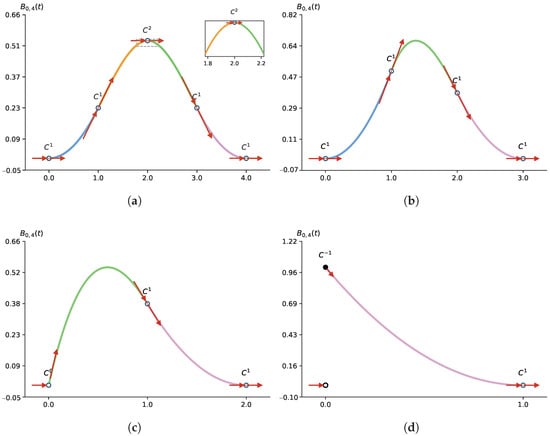
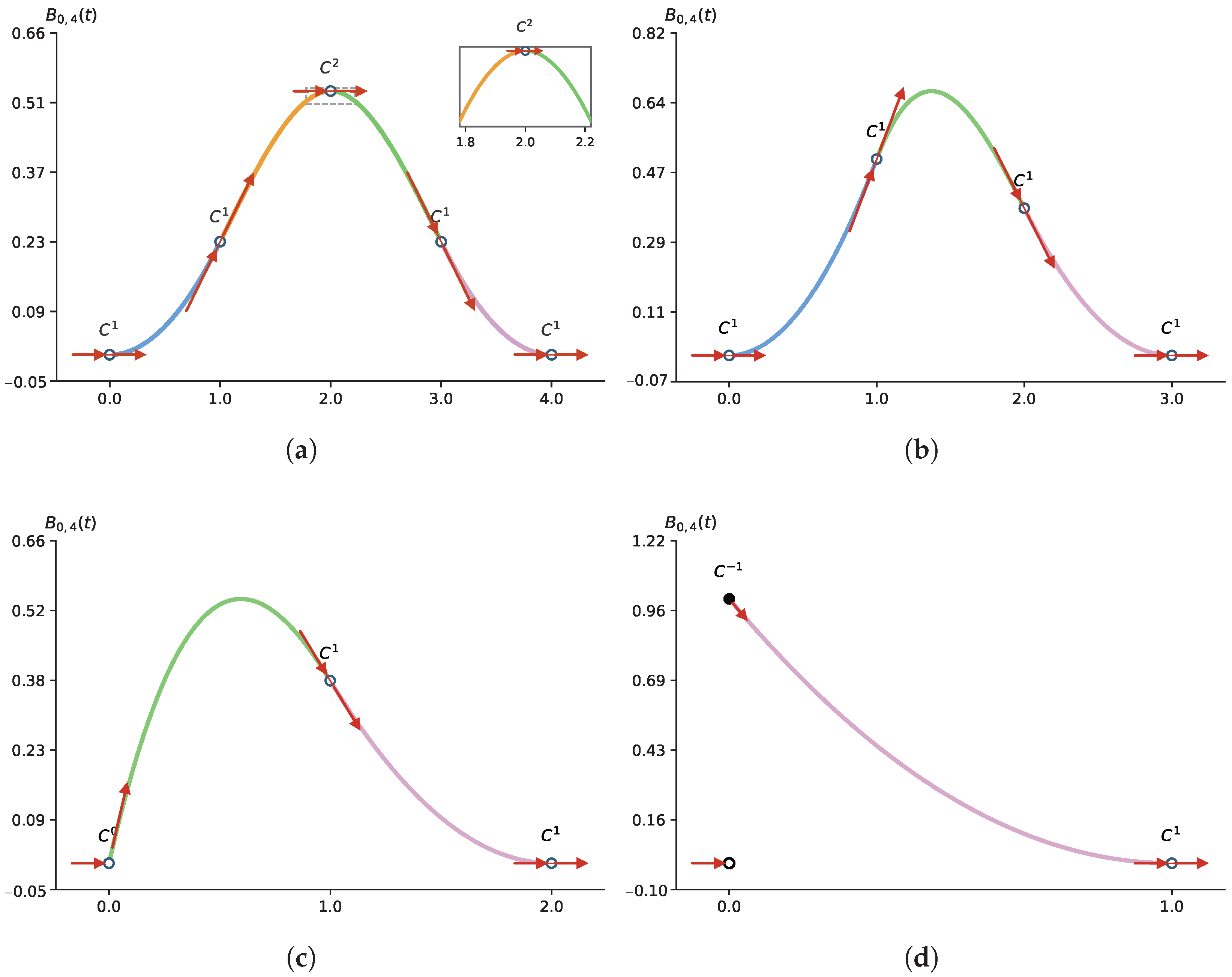
Figure 3 illustrates the continuity relations between adjacent polynomial segments of the Ball-Spline basis function $B_{0,4}\left(t\right)$ under different knot configurations. The arrows indicate the one-sided tangent directions at the knots. In the $C^1$ case, the two neighboring segments share the same tangent vector at the joint. This means that the curve passes through the knot without a break in slope. At the knot $t_2$ in Figure 3a, the adjacent segments not only share the same tangent vector but also exhibit consistent curvature behavior. This corresponds to $C^2$ continuity. In the $C^0$ case, the segments remain connected at the knot, but the tangent vector is not preserved across the joint. In the $C^{-1}$ case, the two segments do not meet at the same point, and therefore the function is discontinuous at the knot.

Figure 3. Continuity properties of the Ball-Spline basis function $B_{0,4}\left(t\right)$ under different knot configurations. (a) $t_0<t_1<t_2<t_3<t_4$; (b) $t_0<t_1=t_2<t_3<t_4$; (c) $t_0=t_1=t_2<t_3<t_4$; (d) $t_0=t_1=t_2=t_3<t_4$. The curves with different colors represent the piecewise polynomial segments of the Ball-Spline basis function $B_{0,4}\left(t\right)$ over consecutive knot intervals.

3. Generalized Ball-Spline Basis Functions

In the previous section, the definition of the Ball-Spline basis functions of order 4 was provided along with proofs of their related properties. In this section, we present the definition of higher-order basis functions.

3.1. Definitions of Generalized Ball-Spline Basis Functions

Definition 2.

Let $\mathit{T}$ be a given knot sequence: ${\left\{t_i\right\}}_{i=-\infty }^{+\infty }$ with $t_i\le t_{i+1}$, $i=0,\pm 1,\dots$. For $k\le 3$, $B_{i,k}\left(t\right),i=0,\pm 1,\dots ,$ are the B-spline basis functions; for $k=4$, $B_{i,4}\left(t\right),i=0,\pm 1,\dots ,$ were already introduced in the preceding section; for $k\ge 5$, $B_{i,k}\left(t\right),i=0,\pm 1,\dots ,$ are defined recursively by $B_{i,4}\left(t\right),i=0,\pm 1,\dots$, i.e., $B_{i,k}\left(t\right)$ are defined by

$$B_{i,k}\left(t\right)={\int }_{-\infty }^t({\delta }_{i,k-1}{B}_{i,k-1}\left(s\right)-{\delta }_{i+1,k-1}{B}_{i+1,k-1}\left(s\right))\mathrm{d}s.$$

(14)

where

$${\delta }_{i,k}=({\int }_{-\infty }^{+\infty }{B}_{i,k}\left(t\right)\mathrm{d}t{)}^{-1}$$

(15)

We call $B_{i,k}\left(t\right),i=0,\pm 1,\dots$ the generalized Ball-Spline basis functions of order k (degree $k-1$). If $t_{j-1}<t_j=t_{j+1}=\dots =t_{j+l-1}<t_{j+l}$, then $t_j,t_{j+1},\dots ,t_{j+l-1}$ are referred to as knots of multiplicity l. We denote the multiplicity of the knot at $t_j$ by $l_j$, where $l_j\ge 1$.

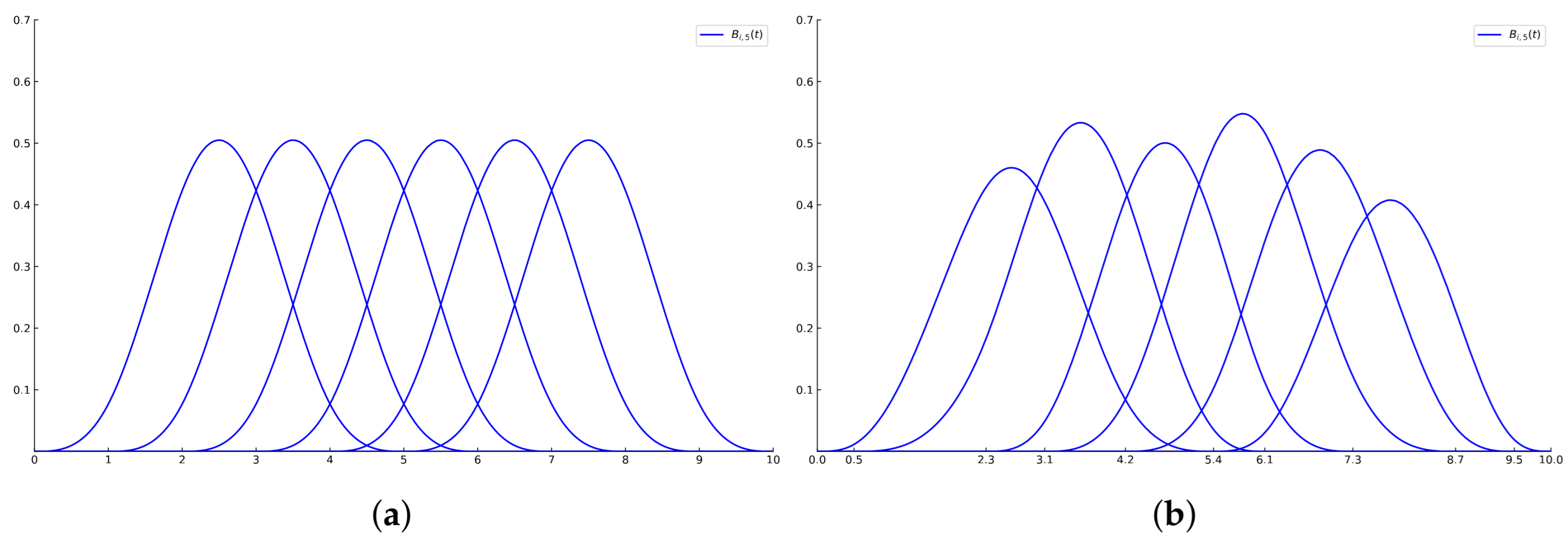
Figure 4 illustrates the generalized Ball-Spline basis functions of order 5.

Figure 4. Generalized Ball-Spline basis functions of order 5. (a) Uniform Ball-Spline basis functions; (b) non-uniform Ball-Spline basis functions.

Remark 5.

From (15), we see that ${{\delta }_{i,k}}^{-1}$ is the area bounded by $B_{i,k}\left(t\right)$ and the parameter axis. When $B_{i,k}\left(t\right)\ne 0$, we have

$${\int }_{-\infty }^{+\infty }{\delta }_{i,k}{B}_{i,k}\left(s\right)\mathrm{d}s=1$$

When $B_{i,k}\left(t\right)=0$, ${\delta }_{i,k}=\infty$. Similar to deBoor-cox, we set ${\delta }_{i,k}{B}_{i,k}\left(s\right)=0$ when $B_{i,k}\left(t\right)=0.$ However, ${\delta }_{i,k}{B}_{i,k}\left(s\right)$ have to satisfy

$${\int }_{-\infty }^{+\infty }{\delta }_{i,k}{B}_{i,k}\left(s\right)\mathrm{d}s=1$$

In order to ensure $B_{i,k}\left(t\right)$ have the normalized property, when $B_{i,k}\left(t\right)=0$, we set

$${\int }_{-\infty }^t{\delta }_{i,k}{B}_{i,k}\left(s\right)\mathrm{d}s=\left\{\begin{array}{c}0,t<t_i,\hfill \\ 1,t\ge t_i.\hfill \end{array}\right.$$

(16)

In fact, ${\delta }_{i,k}{B}_{i,k}\left(s\right)$ are Dirac delta functions when $B_{i,k}\left(t\right)=0$.

3.2. Properties of Generalized Ball-Spline Basis Functions

In this subsection, we will give some basic properties of the functions $B_{i,k}\left(t\right)$. When $k\le 3$, $B_{i,k}\left(t\right)$ are the B-spline basis functions, the following property holds. When $k=4$, the properties of $B_{i,4}\left(t\right)$ have been proved in the previous section. Therefore, the following properties only need to be proven for the case where $k\ge 5$.

Proposition 7

(Local support property). $B_{i,k}\left(t\right)=0,k\ge 5,t\notin [t_i,t_{i+k})$.

Proof. 

We prove this proposition by induction on k. When $k\le 4$, the local support property holds. Assume the proposition holds for $k=m-1,m\ge 5$, then we have

$$B_{i,m-1}\left(t\right)=0,k\ge 5,t\notin [t_i,t_{i+m-1}).$$

For $k=m$, by assumption, when $t<t_i$ or $t\ge t_{i+m}$,

$$B_{i,m-1}\left(t\right)=B_{i+1,m-1}\left(t\right)=0.$$

From (16), when $t<t_i$ and $t\ge t_{i+m}$, we have

$$\begin{array}{cc}\hfill B_{i,m}\left(t\right)& ={\int }_{-\infty }^t{\delta }_{i,m-1}{B}_{i,m-1}\left(s\right)\mathrm{d}s-{\int }_{-\infty }^t{\delta }_{i+1,m-1}{B}_{i+1,m-1}\left(s\right)\mathrm{d}s=0\hfill \end{array}$$

Therefore, $B_{i,m}\left(t\right)=0,t\notin [t_i,t_{i+m})$ holds, i.e., the proposition also holds for $k=m$. □

Proposition 8

(Normalized property). ${\displaystyle \sum _{j=-\infty }^{+\infty }}{B}_{j,k}\left(t\right)\equiv 1$ for $t\in [t_i,t_{i+1})$

Proof. 

For $k\ge 5$, $t\in [t_i,t_{i+1})$, from local support property, we have

$$B_{i-k+1,k-1}\left(t\right)=B_{i+1,k-1}\left(t\right)=0$$

From (16), we have

$$\begin{array}{cc}\hfill {\displaystyle \sum _{j=-\infty }^{+\infty }}{B}_{j,k}\left(t\right)& ={\displaystyle \sum _{j=i-k+1}^i}{B}_{j,k}\left(t\right)\hfill \\ & ={\displaystyle \sum _{j=i-k+1}^i}{\int }_{-\infty }^t{\delta }_{j,k-1}{B}_{j,k-1}\left(s\right)-{\delta }_{j+1,k-1}{B}_{j+1,k-1}\left(s\right)\mathrm{d}s\hfill \\ & ={\int }_{-\infty }^t{\delta }_{i-k+1,k-1}{B}_{i-k+1,k-1}\left(s\right)\mathrm{d}s-{\int }_{-\infty }^t{\delta }_{i+1,k-1}{B}_{i+1,k-1}\left(s\right))\mathrm{d}s\hfill \\ & =1-0=1\hfill \end{array}$$

□

Proposition 9

(Derivative). For $k\ge 5$,

$${\displaystyle \frac{\mathrm{d}}{\mathrm{d}t}}{B}_{i,k}\left(t\right)={\delta }_{i,k-1}{B}_{i,k-1}\left(t\right)-{\delta }_{i+1,k-1}{B}_{i+1,k-1}\left(t\right)$$

Proposition 10

(Linear independence).

(1) 

$B_{i-k+1,k}\left(t\right),B_{i-k+2,k}\left(t\right),\dots ,B_{i-1,k}\left(t\right),B_{i,k}\left(t\right)$ are linearly independent on $[t_i,t_{i+1})$ for all i.

(2) 

The functions ${\left\{B_{i,k}\left(t\right)\right\}}_{i=-\infty }^{+\infty }$ are linearly independent on $(-\infty ,+\infty )$.

Proof. 

We prove (1), and (2) follows easily from (1). We prove this proposition by induction on k. When $k\le 4$, the linear independence property holds. Assume the proposition holds for $k-1,k\ge 5$, let

$$\phi \left(t\right)={\displaystyle \sum _{j=i-k+1}^i}{\alpha }_j{B}_{j,k}\left(t\right)=0$$

The derivative of $\phi \left(t\right)$ is

$$\begin{array}{cc}\hfill {\phi }^{\prime }\left(t\right)& ={\displaystyle \sum _{j=i-k+1}^i}{\alpha }_j({\delta }_{j,k-1}{B}_{j,k-1}\left(t\right)-{\delta }_{j+1,k-1}{B}_{j+1,k-1}\left(t\right))\hfill \\ & ={\displaystyle \sum _{j=i-k+2}^i}({\alpha }_j-{\alpha }_{j-1}){\delta }_{j,k-1}{B}_{j,k-1}\left(t\right)=0\hfill \end{array}$$

By assumption, $B_{i-k+2,k-1}\left(t\right),B_{i-k+3,k-1}\left(t\right),\dots ,B_{i,k-1}\left(t\right)$ are linearly independent on $[t_i,t_{i+1})$, then we have

$${\alpha }_j-{\alpha }_{j-1}=0,j=i-k+2,\dots ,i$$

i.e.,

$${\alpha }_{i-k+1}={\alpha }_{i-k+2}=\dots ={\alpha }_{i-1}={\alpha }_i$$

Due to the normalized property,

$$\phi \left(t\right)={\displaystyle \sum _{j=i-k+1}^i}{\alpha }_j{B}_{j,k}\left(t\right)={\alpha }_i{\displaystyle \sum _{j=i-k+1}^i}{B}_{j,k}\left(t\right)={\alpha }_i=0$$

This means that the proposition holds for k. □

Proposition 11

(Positivity Property). $B_{i,k}\left(t\right)>0$ for $t\in (t_i,t_{i+k})$

Proof. 

We prove this proposition by induction on k. When $k\le 4$, the positivity property holds. Assume the proposition holds for $k-1,k\ge 5$, i.e., $B_{i,k-1}\left(t\right)>0,t\in (t_i,t_{i+k-1})$ for all i. Set

$$H_{i,k-1}\left(t\right)={\int }_{-\infty }^t{\delta }_{i,k-1}{B}_{i,k-1}\left(s\right)\mathrm{d}s={\displaystyle \frac{{\int }_{-\infty }^t{B}_{i,k-1}\left(s\right)\mathrm{d}s}{{\int }_{-\infty }^{+\infty }{B}_{i,k-1}\left(t\right)\mathrm{d}t}},$$

then, due to translation property, we have

$$H_{i+1,k-1}\left(t\right)={\displaystyle \frac{{\int }_{-\infty }^t{B}_{i+1,k-1}\left(s\right)\mathrm{d}s}{{\int }_{-\infty }^{+\infty }{B}_{i+1,k-1}\left(t\right)\mathrm{d}t}},$$

and

$$B_{i,k}\left(t\right)=H_{i,k-1}\left(t\right)-H_{i+1,k-1}\left(t\right).$$

By assumption, $H_{j,k-1}\left(t\right)$ is monotonically increasing with respect to t, and

$$H_{j,k-1}\left(t\right)\left\{\begin{array}{ccc}=0,\hfill & & t\le t_j,\hfill \\ \in (0,1),\hfill & & t\in (t_j,t_{j+k-1}),\hfill \\ =1,\hfill & & t\ge t_{j+k-1},\hfill \end{array}\right.j=i,i+1.$$

For $t\in (t_i,t_{i+k})$, when $t\in (t_i,t_{i+1})$,

$$B_{i,k}\left(t\right)=H_{i,k-1}\left(t\right)>0.$$

When $t\in [t_{i+k-1},t_{i+k})$,

$$B_{i,k}\left(t\right)=1-H_{i+1,k-1}\left(t\right)>0.$$

When $t\in [t_{i+1},t_{i+k-1})$, apply a linear transformation:

$$u=f\left(t\right)=a_{j}t+b_j,t\in (t_i,t_{i+1})\cup [t_{i+j},t_{i+j+1}),$$

(17)

where

$$a_j={\displaystyle \frac{1}{t_{i+j+1}-t_{i+j}}},b_j={\displaystyle \frac{j{t}_{i+j+1}-(j+1)t_{i+j}}{t_{i+j+1}-t_{i+j}}}.j=1,\dots ,k-1,$$

i.e.,

$$u=f\left(t\right)=\left\{\begin{array}{c}{\displaystyle \frac{-t_i}{t_{i+1}-t_i}}+{\displaystyle \frac{t}{t_{i+1}-t_i}},t\in (t_i,t_{i+1}),\hfill \\ {\displaystyle \frac{t_{i+2}-2t_{i+1}}{t_{i+2}-t_{i+1}}}+{\displaystyle \frac{t}{t_{i+2}-t_{i+1}}},t\in [t_{i+1},t_{i+2}),\hfill \\ ⋮\hfill \\ {\displaystyle \frac{j{t}_{i+j+1}-(j+1)t_{i+j}}{t_{i+j+1}-t_{i+j}}}+{\displaystyle \frac{t}{t_{i+j+1}-t_{i+j}}},t\in [t_{i+j},t_{i+j+1}),\hfill \\ ⋮\hfill \\ {\displaystyle \frac{(k-2)t_{i+k-1}-(k-1)t_{i+k-2}}{t_{i+k-1}-t_{i+k-2}}}+{\displaystyle \frac{t}{t_{i+k-1}-t_{i+k-2}}},t\in [t_{i+k-2},t_{i+k-1}),\hfill \\ {\displaystyle \frac{(k-1)t_{i+k}-k{t}_{i+k-1}}{t_{i+k}-t_{i+k-1}}}+{\displaystyle \frac{t}{t_{i+k}-t_{i+k-1}}},t\in [t_{i+k-2},t_{i+k-1}).\hfill \end{array}\right.$$

(18)

The knot sequences $\mathit{U}={\left\{u_i\right\}}_{i=-\infty }^{+\infty }$ obtained by transformation (17) are uniform knot sequences, which satisfy

$$\begin{array}{c}\hfill u_i=f\left(t_i\right)=0,u_{i+1}=f\left(t_{i+1}\right)=1,\dots ,u_{i+k-1}=f\left(t_{i+k-1}\right)=k-1.\end{array}$$

Let

$$H_{i,k-1}\left(t\right)=F(t;t_i,t_{i+1},\dots ,t_{i+k-1}),$$

due to (18) and the translation property, we have

$$\begin{array}{cc}\hfill H_{i,k-1}\left(t\right)& =F(t;t_i,t_{i+1},\dots ,t_{i+k-1})\hfill \\ & =F(f^{-1}\left(u\right);f^{-1}\left(0\right),f^{-1}\left(1\right),\dots ,f^{-1}(k-1))\stackrel{\Delta }{=}G(u;0,1,\dots ,k-1)\hfill \\ \hfill H_{i+1,k-1}\left(t\right)& =F(t;t_{i+1},t_{i+2},\dots ,t_{i+k})\hfill \\ & =F(f^{-1}\left(u\right);f^{-1}\left(1\right),f^{-1}\left(2\right),\dots ,f^{-1}\left(k\right))\stackrel{\Delta }{=}G(u;1,2,\dots ,k)\hfill \end{array}$$

For any $u^{*}\in [u_{i+j},u_{i+j+1}),j=1,2,\dots ,k-2,$ there exists $u^{\prime }=u^{*}+1,u^{\prime }\in [u_{i+j+1},u_{i+j+2}),j=1,2,\dots ,k-2,$ such that

$$G(u^{*};0,1,\dots ,k-1)=G(u^{\prime };1,2,\dots ,k).$$

Then for any $t^{*}=f^{-1}\left(u^{*}\right),t^{*}\in [t_{i+j},t_{i+j+1}),j=1,2,\dots ,k-2,$ there exists $t^{\prime }$, such that

$$\begin{array}{cc}\hfill H_{i,k-1}\left(t^{*}\right)& =G(u^{*};0,1,\dots ,k-1)\hfill \\ & =G(u^{\prime };1,2,\dots ,k)=F(t^{\prime };t_{i+1},t_{i+2},\dots ,t_{i+k})=H_{i+1,k-1}\left(t^{\prime }\right),\hfill \end{array}$$

where

$$t^{\prime }={\displaystyle \frac{a_j{t}^{*}+b_j-b_{j+1}+1}{a_{j+1}}}.$$

Substituting $a_j$ and $b_j$ into $t^{\prime }$ yields

$$t^{\prime }={\displaystyle \frac{t_{i+j+2}-t_{i+j+1}}{t_{i+j+1}-t_{i+j}}}(t^{*}-t_{i+j})+t_{i+j+1}\ge t_{i+j+1}>t^{*}.$$

Therefore

$$\begin{array}{cc}\hfill B_{i,k}\left(t^{*}\right)& =H_{i,k-1}\left(t^{*}\right)-H_{i+1,k-1}\left(t^{*}\right)=H_{i+1,k-1}\left(t^{\prime }\right)-H_{i+1,k-1}\left(t^{*}\right)>0.\hfill \end{array}$$

By the arbitrariness of $t^{*}$, we conclude that $\forall t\in [t_{i+1},t_{i+k-1}),B_{i,k}\left(t\right)>0.$ Hence, $B_{i,k}\left(t\right)>0$ for $t\in (t_i,t_{i+k})$. □

Proposition 12

(Continuity). The continuity order of $B_{i,k}\left(t\right),k\ge 5,i=0,\pm 1,\dots ,$ at $t_j$ (where $i\le j\le i+k$) can be categorized as follows:

(i) 

When $t_i<t_{i+1}<\dots <t_{i+k-1}<t_{i+k}$, $B_{i,k}\left(t\right)$ is $C^{k-3}$ at $t_j,j=i,i+1,\dots ,i+k$.

(ii) 

When $t_i=t_{i+1}=\dots =t_{i+\xi -1}<t_{i+\xi }\le t_{i+\xi +1}\le \dots \le t_{i+k-\eta }<t_{i+k-\eta +1}=t_{i+k-\eta +2}=\dots =t_{i+k}$, $\xi ,\eta ,l_j\ge 2$, $B_{i,k}\left(t\right)$ is $C^{m_j}$ at $t_j$, where

$$m_j=\left\{\begin{array}{ccc}k-1-\xi ,\hfill & & i\le j\le i+\xi -1,\hfill \\ k-1-l_j,\hfill & & i+\xi \le j\le i+k-\eta ,\hfill \\ k-1-\eta ,\hfill & & i+k-\eta +1\le j\le i+k.\hfill \end{array}\right.$$

Proof. 

Based on the integral recurrence definition of $B_{i,k}\left(t\right),k\ge 5$, where each integration increases the continuity order by one, the continuity properties of $B_{i,k}\left(t\right),k\ge 5$ can be directly deduced from the continuity analysis of $B_{i,4}\left(t\right)$ presented in Proposition 6. □

4. Generalized Ball-Spline Curves

4.1. Definitions of Generalized Ball-Spline Curves

Generalized Ball-Spline curves are constructed based on generalized Ball-Spline basis functions.

Definition 3.

Given a point sequence ${\left\{{\mathit{P}}_{\mathit{i}}\right\}}_{i=1}^n$, the corresponding generalized Ball-Spline curve over $\mathit{T}$ is defined by

$$\mathit{P}\left(t\right)={\displaystyle \sum _{i=1}^n}{B}_{i,k}\left(t\right){\mathit{P}}_{\mathit{i}},t\in \left[t_k,t_{n+1}\right],n\ge k$$

(19)

Here, the point sequence ${\left\{{\mathit{P}}_{\mathit{i}}\right\}}_{i=1}^n$ and the polygon ${\mathit{P}}_{\mathsf{1}}{\mathit{P}}_{\mathsf{2}}\dots {\mathit{P}}_{\mathit{n}}$ are, respectively, called the control points and the control polygon of the generalized Ball-Spline curve (19).

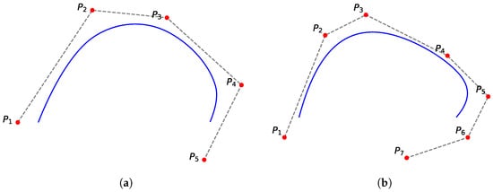
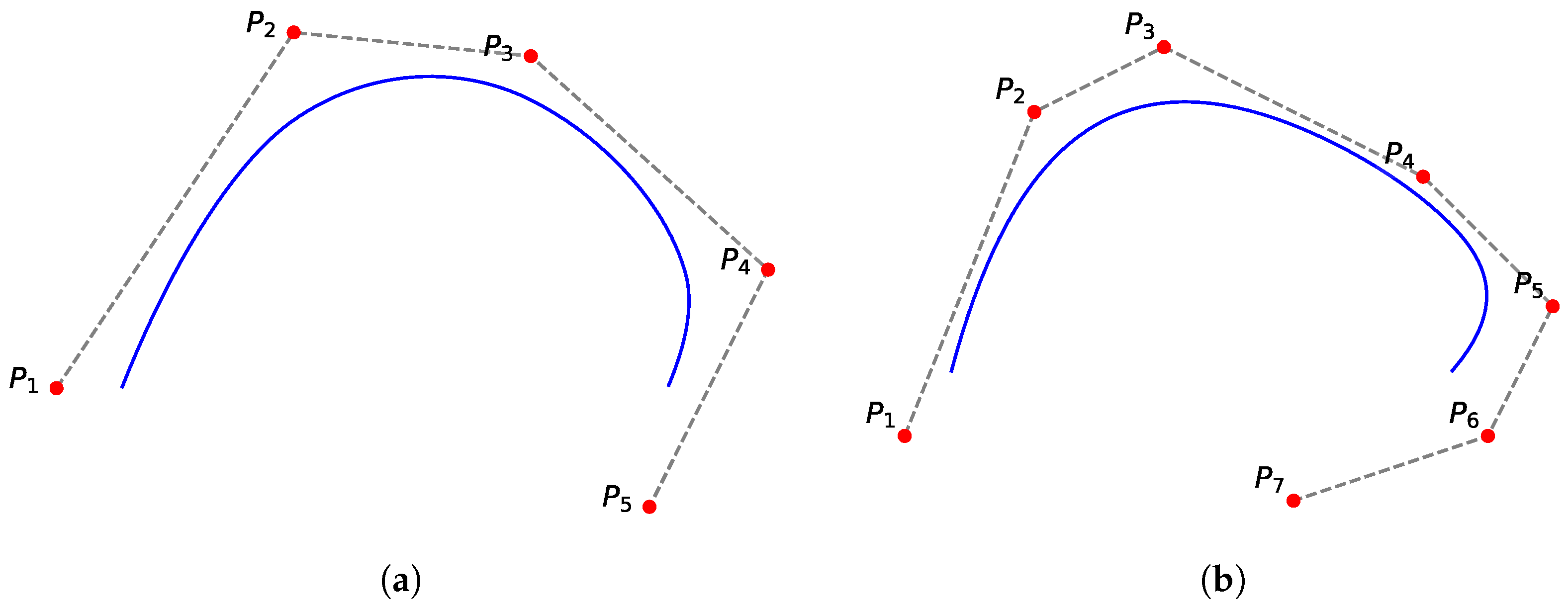
Figure 5 illustrates the generalized Ball-Spline curves for $k=4$ and $k=5$.

Figure 5. Generalized Ball-Spline curves. (a) k = 4; (b) k = 5.

4.2. Properties of Generalized Ball-Spline Curves

The properties of the generalized Ball-Spline curve can be directly derived from its basis functions. According to Definition 3, the curve possesses the following properties.

Proposition 13

(Convex Hull Property). The generalized Ball-Spline curve $\mathit{P}\left(t\right)$ lies inside the convex hull of its control polygon.

Proposition 14

(Geometric Invariance Property). The shape of generalized Ball-Spline curve is independent of the choice of coordinate system.

Proposition 15

(Derivative Curve). The derivative curve of $\mathit{P}\left(t\right)$ is

$$\begin{array}{c}\hfill {\displaystyle \frac{\mathrm{d}}{\mathrm{d}t}}\mathit{P}\left(t\right)={\displaystyle \sum _{i=2}^n}{\delta }_{i,k-1}{B}_{i,k-1}\left(t\right)\Delta {\mathit{P}}_{\mathit{i}},t\in \left[t_k,t_{n+1}\right],k\ge 5.\end{array}$$

where $\Delta {\mathit{P}}_{\mathit{i}}={\mathit{P}}_{\mathit{i}}-{\mathit{P}}_{\mathit{i}-\mathsf{1}}$.

Proposition 16

(Local Control Property). Changing one of the control points ${\mathit{P}}_{\mathit{i}}$ will alter at most k segments of the original Generalized Ball-Spline curve.

From this property, we see that local adjustment can be made without disturbing the rest of the curve.

Proposition 17

(Relation with Ball curve). For generalized Ball-Spline curve of order 4,

$$\mathit{P}\left(t\right)={\displaystyle \sum _{i=1}^n}{B}_{i,4}\left(t\right){\mathit{P}}_{\mathit{i}},t\in \left[t_4,t_{n+1}\right],n\ge 4,$$

if $t_{i-3}=t_{i-2}=t_{i-1}=t_i<t_{i+1}=t_{i+2}=t_{i+3}=t_{i+4}$, the generalized Ball-Spline curve $\mathit{P}\left(t\right)$ is just a Ball curve of degree 3 on the interval $[t_i,t_{i+1}]$.

Proposition 18

(Continuity). For $j\in [k,n+1]$, if $t_j$ is a knot of multiplicity $l_j$ with $t_{j-1}<t_j=\dots =t_{j+l_j-1}<t_{j+l_j}$, then the generalized Ball-Spline curve $\mathit{P}\left(t\right)$ is at least $C^{m_j}$ at $t_j$, where

$$m_j=\left\{\begin{array}{ccc}k-3,\hfill & & l_j=1,\hfill \\ k-1-l_j,\hfill & & l_j\ge 2.\hfill \end{array}\right.$$

4.3. Geometric and Physical Interpretation of Curve Properties

The mathematical properties of generalized Ball-Spline curves admit natural geometric interpretations, which help to explain their behavior in practical modeling contexts.

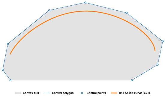
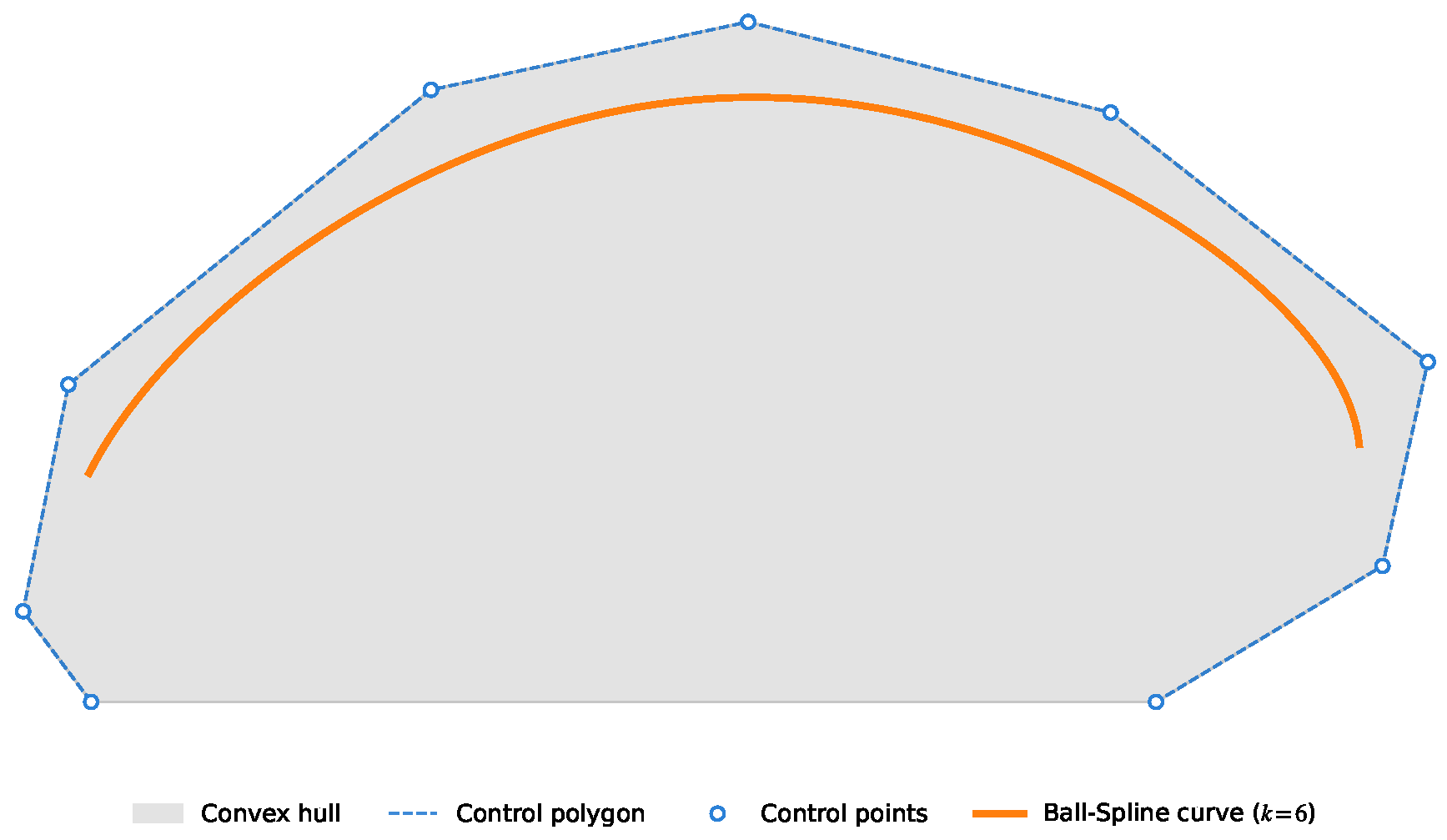
As shown in Figure 6, the convex hull property indicates that the curve lies entirely within the convex hull of its control polygon. From a geometric and physical point of view, this indicates that the behavior of the resulting curve is closely related to the configuration of the control points. Changes in the control polygon lead to corresponding changes in the curve within the same region, which limits the deviation of the curve from the control polygon.

Figure 6. Convex hull property of the generalized Ball-Spline curve.

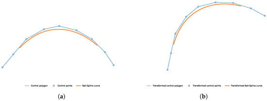
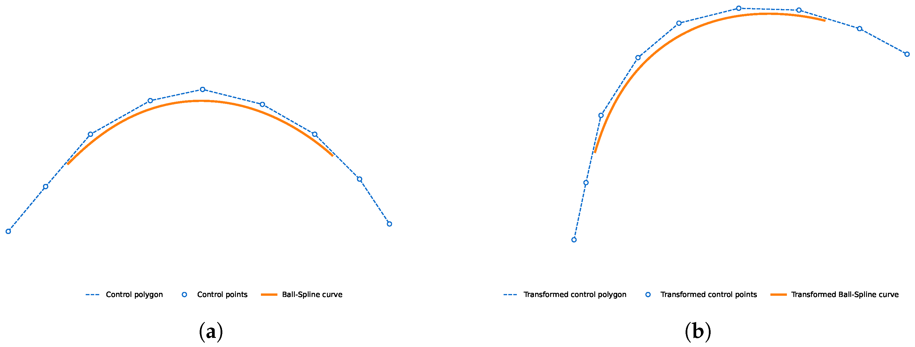
The geometric invariance property means that when the control points are transformed by an affine transformation, such as translation, rotation, or scaling, the curve changes in the same way, while its shape remains the same. As shown in Figure 7, the left image presents the control polygon and the curve in the original coordinate system, and the right image shows the result after transformation. It can be seen that the relative position between the curve and the control polygon is preserved. The shape of the curve does not change, and only its overall position and orientation are transformed.

Figure 7. Geometric invariance under affine transformations. (a) Original configuration; (b) affine transformation.

From a geometric and physical point of view, this indicates that the resulting curve representation is independent of the choice of coordinate system. The curve keeps its intrinsic shape under rigid motions and scaling, which is consistent with the behavior of geometric objects in physical space.

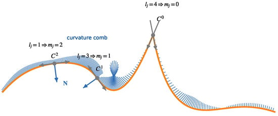
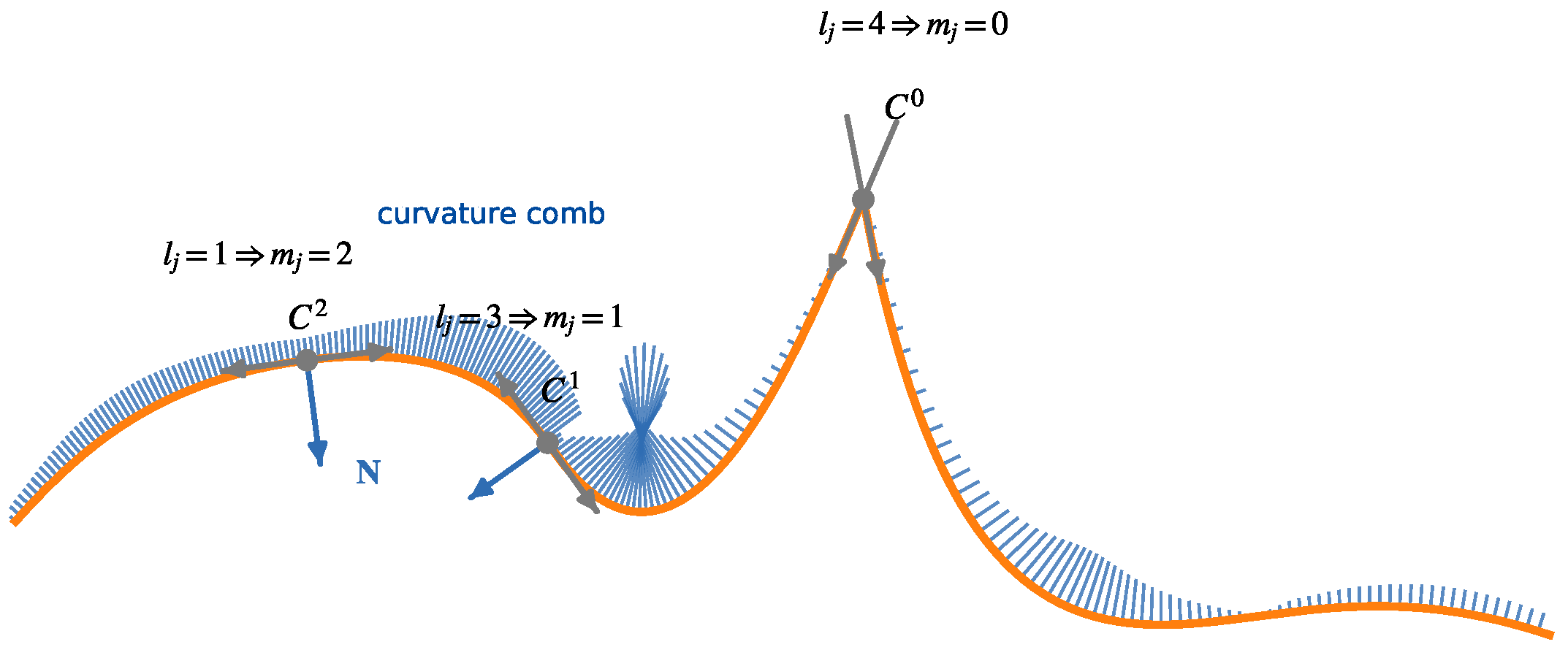
The continuity of the curve depends on the multiplicity of the knots. Figure 8 shows a 5th-order generalized Ball-Spline curve for different knot multiplicities, corresponding to $C^2$, $C^1$, and $C^0$ continuity. The figure includes one-sided tangent directions and a curvature comb. Let $\mathit{P}\left(t\right)=\left(x\right(t),y(t\left)\right)$ be a parametric curve. Its first and second derivatives are

$${\mathit{P}}^{\prime }\left(t\right)={\displaystyle \sum _{i=1}^n}{B}_{i,k}^{\prime }\left(t\right){\mathit{P}}_i,{\mathit{P}}^{″}\left(t\right)={\displaystyle \sum _{i=1}^n}{B}_{i,k}^{″}\left(t\right){\mathit{P}}_i.$$

These derivatives determine the tangent direction and enter the expression of the curvature. The curvature is given by

$$\kappa \left(t\right)={\displaystyle \frac{x^{\prime }\left(t\right)y^{″}\left(t\right)-y^{\prime }\left(t\right)x^{″}\left(t\right)}{{\left(x^{\prime }{\left(t\right)}^2+y^{\prime }{\left(t\right)}^2\right)}^{3/2}}},$$

and the unit normal vector is

$$\mathit{N}\left(t\right)={\displaystyle \frac{(-y^{\prime }\left(t\right),x^{\prime }\left(t\right))}{\sqrt{x^{\prime }{\left(t\right)}^2+y^{\prime }{\left(t\right)}^2}}}.$$

The curvature comb is defined by

$$\mathit{P}\left(t\right)+s\kappa \left(t\right)\mathit{N}\left(t\right),$$

where $s>0$ is a scaling parameter. Thus, the length of each comb segment is proportional to the magnitude of the curvature, and its direction is determined by the normal vector. As shown in Figure 8, in the $C^2$ case, the one-sided tangent directions coincide at the knot, and the curvature comb varies continuously in its neighborhood. In the $C^1$ case, the one-sided tangent directions still coincide, but the curvature comb shows a visible change near the knot. In the $C^0$ case, the one-sided tangent directions do not coincide, and the curve forms a corner at the knot. Therefore, the figure provides a geometric visualization of the change in bending behavior under different continuity conditions.

Figure 8. Continuity of the generalized Ball-Spline curve.

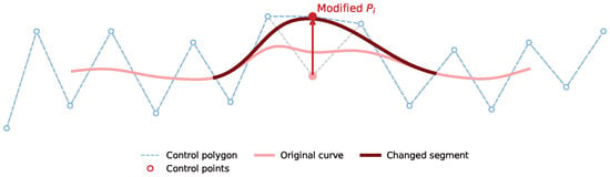
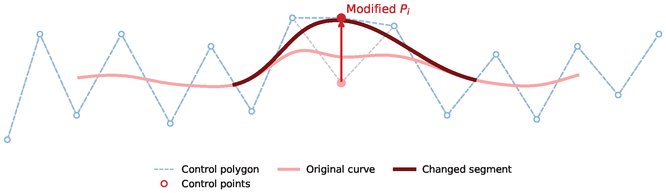
The local control property indicates that each control point affects only a limited portion of the curve. Therefore, modifying one control point changes only a local segment, while the remaining parts stay unchanged. As shown in Figure 9, when a control point is moved, only a segment in its neighborhood (the darker curve) is affected, while the parts far from this point remain almost unchanged. From a geometric and physical point of view, this indicates that the influence of each control point is local. A local change in the control polygon leads to a local change in the curve. This allows local adjustment without changing the overall shape. Such behavior is useful in shape editing and interactive modeling, where only a small region needs to be modified.

Figure 9. Local control property of the generalized Ball-Spline curve.

The derivative expression shows that the derivative of the curve is expressed in terms of the differences $\Delta {\mathit{P}}_{\mathit{i}}={\mathit{P}}_{\mathit{i}}-{\mathit{P}}_{\mathit{i}-\mathsf{1}}$ and the basis functions of order $k-1$. The relation with the classical Ball curve shows that, under specific knot configurations, the generalized Ball-Spline curve reduces to the cubic Ball curve on a subinterval. This follows from Proposition 4. Therefore, the proposed curve of order 4 is consistent with the classical Ball curve in these cases.

4.4. Examples

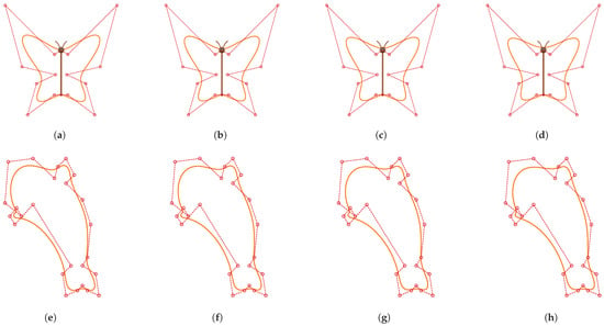
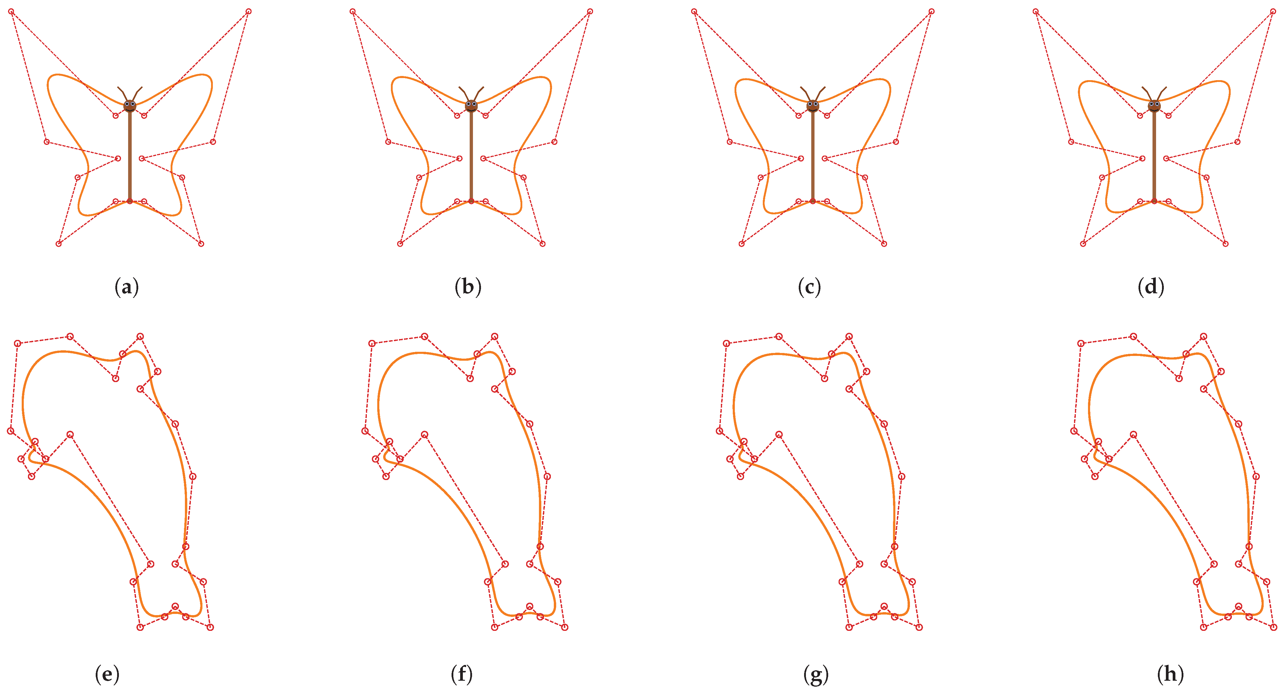
Figure 10 presents butterfly and dolphin contours generated by Ball-Spline curves with orders 7, 8, 9, and 10, along with their corresponding control polygons.

Figure 10. Two examples of Ball-Spline curves. (a) butterfly (k = 7); (b) butterfly (k = 8); (c) butterfly (k = 9); (d)butterfly (k = 10); (e) dolphin (k = 7); (f) dolphin (k = 8); (g) dolphin (k = 9); (h) dolphin (k = 10).

4.5. Comparison of Control Point Requirements for the Given Accuracy

To compare the control point requirements of Ball-Spline and B-spline under the same approximation accuracy constraint, the Ball-Spline curve is taken as the reference curve, and the B-spline curve is obtained through RMSE-based fitting. Let K sampling parameters ${\left\{{\xi }_k\right\}}_{k=1}^K$ be selected over the parameter domain, where K is set to 6000. Denote the Ball-Spline curve and the B-spline curve by

$${\mathit{P}}_{Ball}\left(t\right),{\mathit{P}}_B\left(t\right),$$

respectively. At each sampling parameter ${\xi }_k$, the pointwise deviation between the two curves is defined as

$$e_k={∥{\mathit{P}}_B\left({\xi }_k\right)-{\mathit{P}}_{\mathit{Ball}}\left({\xi }_k\right)∥}_2,$$

where ${\parallel ·\parallel }_2$ denotes the Euclidean norm in ${\mathbb{R}}^2$. The root mean square error (RMSE) is then defined as

$$\mathrm{RMSE}=\sqrt{{\displaystyle \frac{1}{K}}\sum _{k=1}^K{∥{\mathit{P}}_B\left({\xi }_k\right)-{\mathit{P}}_{Ball}\left({\xi }_k\right)∥}_2^2}.$$

This quantity measures the average geometric deviation between the two curves over the sampled parameter values. A smaller RMSE indicates a closer agreement in overall shape. In the experiments, the error threshold is set to 0.01, and RMSE is used as the evaluation metric. When the RMSE between the B-spline curve and the reference curve is less than 0.01, the approximation is considered acceptable. Under this unified error threshold, the required numbers of control points are compared.

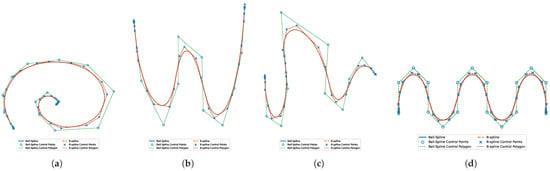
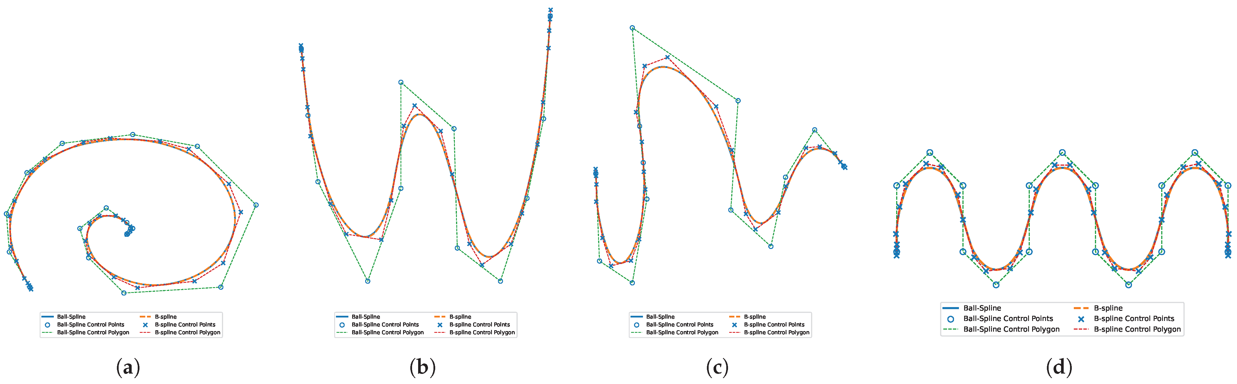
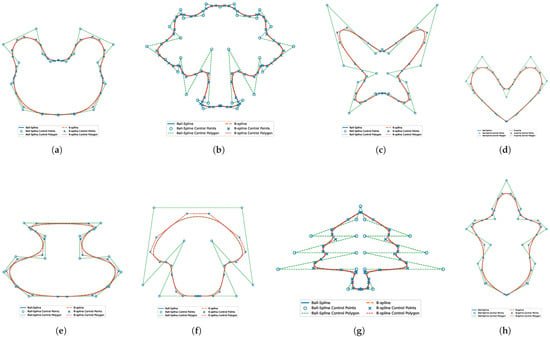
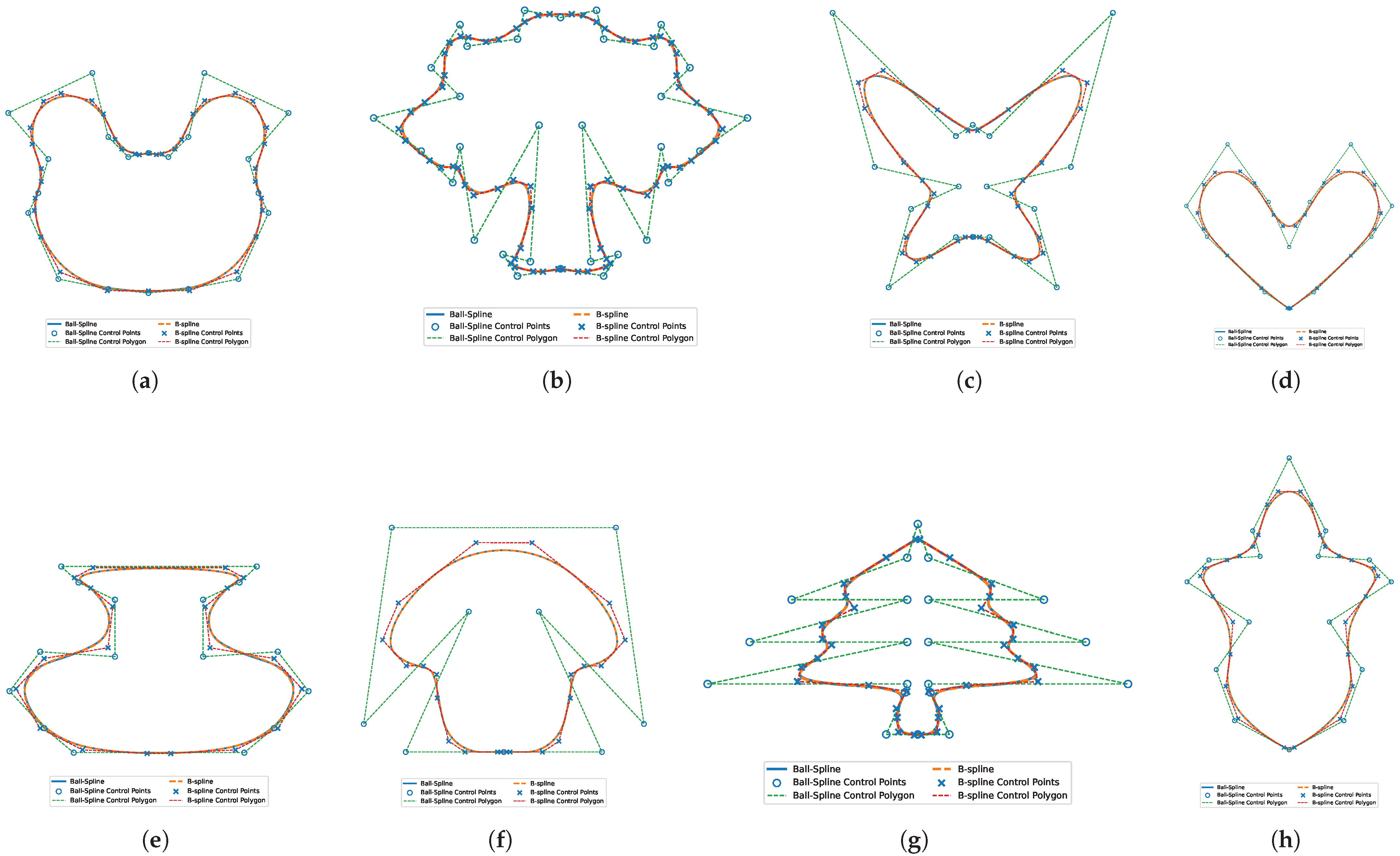
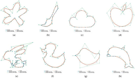
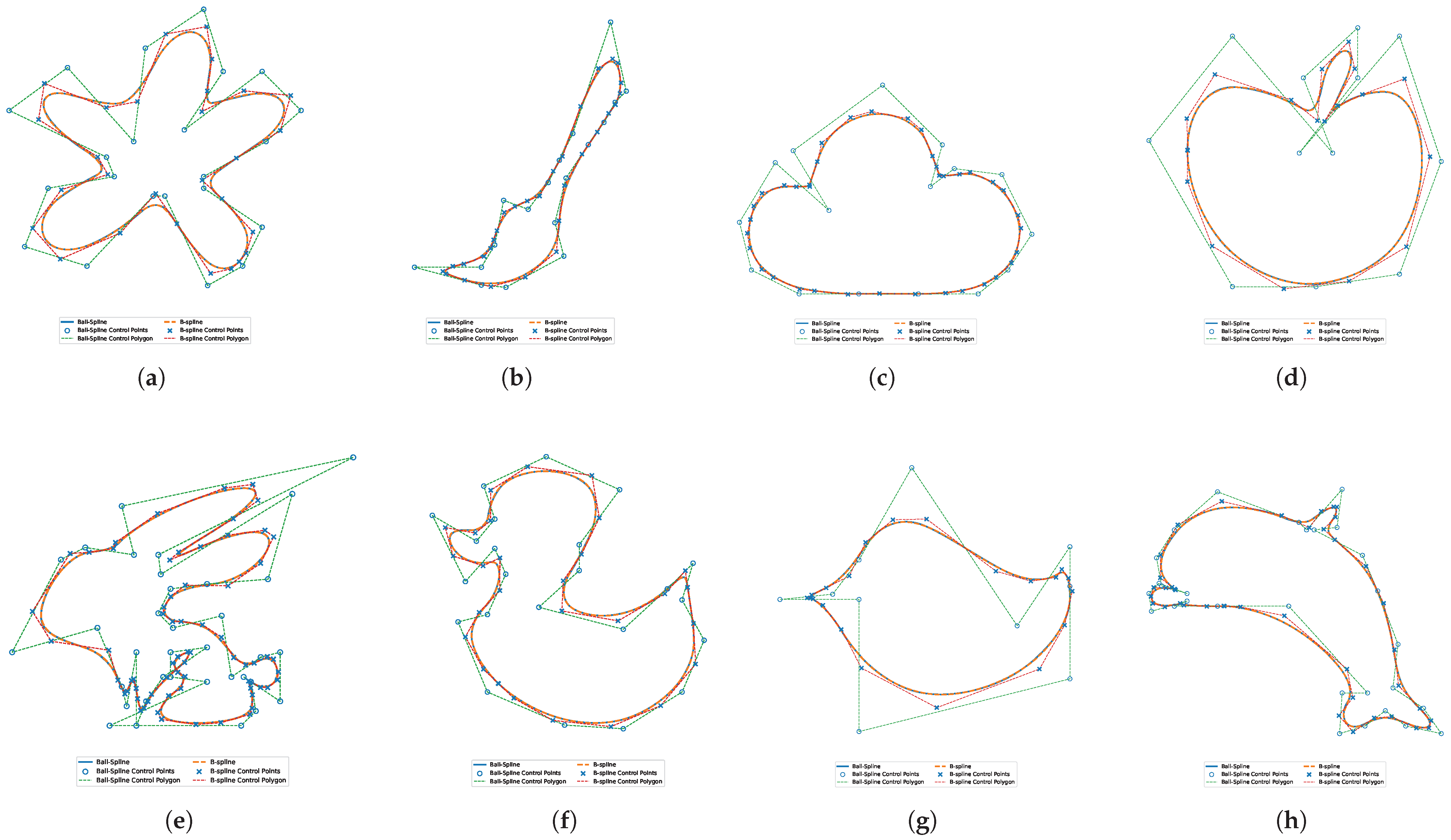
Since cubic Ball basis functions are more commonly used in practical geometric modeling than their higher-order counterparts, the experimental comparison in this work focuses on cubic curves. According to their geometric characteristics, symmetry properties, and boundary conditions, the test curves are categorized into three groups: open curves (Figure 11), symmetric closed curves (Figure 12), and asymmetric closed curves (Figure 13). To ensure a fair comparison, the same parameter partition is adopted for both representations. After removing duplicated knots, the two curve models share an identical knot sequence and the same number of non-zero knot intervals. As reported in Table 1, Table 2 and Table 3, under the prescribed error threshold, the Ball-Spline representation achieves a fitting accuracy comparable to that of the B-spline curve while requiring fewer control points.

Figure 11. Open curves. (a) open curve 1; (b) open curve 2; (c) open curve 3; (d) open curve 4.

Figure 12. Closed symmetric curves. (a) bear; (b) tree; (c) butterfly; (d) heart shape; (e) vase; (f) mushroom; (g) pine; (h) hazelnut.

Figure 13. Closed asymmetric curves: (a) flower; (b) paintbrush; (c) cloud; (d) apple; (e) rabbit; (f) duck; (g) bird; (h) dolphin.

Table 1. Numbers of control points and non-zero knot intervals for open curves.

	Open Curve 1	Open Curve 2	Open Curve 3	Open Curve 4
Ball-Spline	17	12	13	17
B-spline	34	26	28	36
RMSE	0.0061	0.0097	0.0086	0.0074
Knot intervals	17	12	13	17

Table 2. Numbers of control points and non-zero knot intervals for closed symmetric curves.

	Bear	Tree	Butterfly	Heart Shape	Vase	Mushroom	Pine	Hazelnut	Egg
Ball-Spline	20	33	16	12	16	10	21	17	10
B-spline	36	66	31	23	20	22	34	28	15
RMSE	0.0095	0.0079	0.0095	0.0084	0.0074	0.0080	0.0076	0.0084	0.0098
Knot intervals	23	36	19	16	19	12	23	19	13

Table 3. Numbers of control points and non-zero knot intervals for closed asymmetric curves.

	Flower	Paintbrush	Cloud	Apple	Rabbit	Duck	Bird	Dolphin
Ball-Spline	22	18	16	12	35	23	10	29
B-spline	29	31	39	19	69	29	22	41
RMSE	0.0094	0.0098	0.0099	0.0098	0.0097	0.0079	0.0089	0.0099
Knot intervals	25	21	19	15	38	26	13	32

It should be noted that this observation is made under the present experimental settings and error threshold, and does not imply superiority in all scenarios. The required number of control points may also depend on curve complexity.

4.6. Comparison of Computational Cost Between Ball-Spline and B-Spline Curves

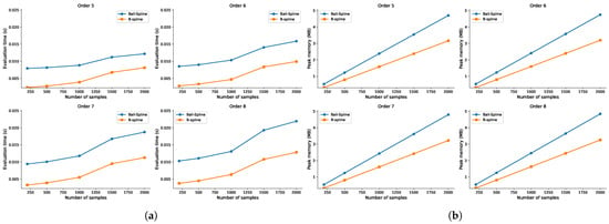
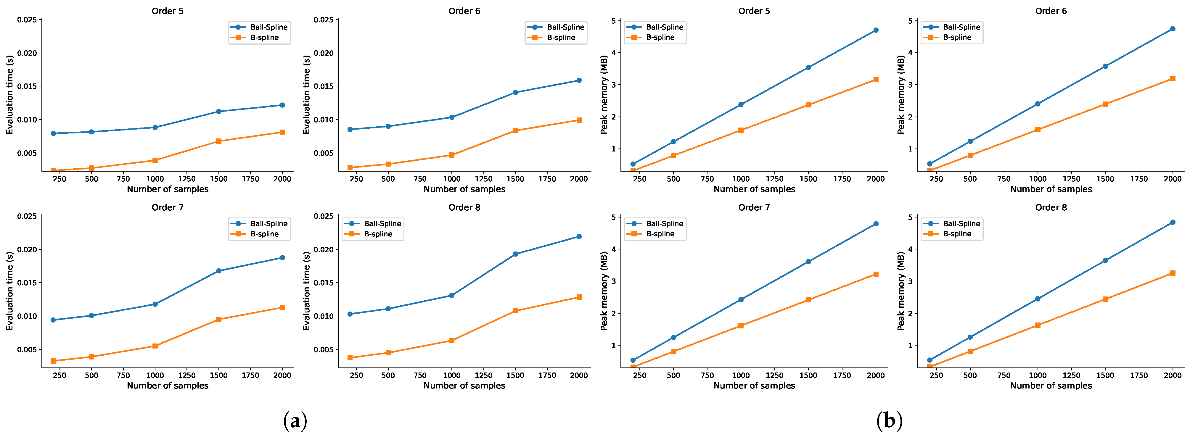
To compare the computational cost of Ball-Spline curves and classical B-spline curves, we evaluate the runtime and peak memory under the same control points, knot sequence, spline order, and sampling density. For each configuration, parameter values are uniformly sampled over the valid parameter domain. The curve points are evaluated point by point. The runtime and peak memory are recorded during the evaluation process. The results are shown in Figure 14 and Table 4. As the number of sampling points increases, the evaluation time of both methods grows approximately linearly. The results show that, under the same conditions, Ball-Spline curves require slightly more evaluation time and memory than B-splines. This difference is mainly caused by the construction of the basis functions. B-splines use the efficient de Boor–Cox recursion. In contrast, the higher-order Ball-Spline basis functions are constructed by an integral recurrence. This process introduces additional computations. Therefore, in the current implementation, the evaluation time and memory consumption are slightly higher.

Figure 14. Comparison of computational cost. (a) Time comparison; (b) memory comparison.

Table 4. Comparison of evaluation time and memory consumption.

Order	Samples	Ball-Spline Time (s)	B-Spline Time (s)	Ball-Spline Memory (MB)	B-Spline Memory (MB)
5	200	0.00793	0.002359	0.527	0.317
	500	0.008156	0.002752	1.223	0.792
	1000	0.008823	0.003887	2.382	1.582
	1500	0.01121	0.006764	3.542	2.372
	2000	0.01218	0.008118	4.702	3.162
6	200	0.008526	0.002795	0.531	0.321
	500	0.008989	0.003330	1.234	0.799
	1000	0.01034	0.004675	2.405	1.597
	1500	0.01407	0.008356	3.577	2.395
	2000	0.01587	0.009924	4.748	3.192
7	200	0.009402	0.003254	0.536	0.324
	500	0.01006	0.003885	1.246	0.807
	1000	0.01177	0.005502	2.428	1.612
	1500	0.01677	0.009497	3.611	2.418
	2000	0.01874	0.01127	4.793	3.223
8	200	0.01030	0.003741	0.541	0.327
	500	0.01108	0.004488	1.257	0.814
	1000	0.01309	0.006322	2.451	1.627
	1500	0.01928	0.01076	3.645	2.440
	2000	0.02193	0.01283	4.839	3.253

4.7. Numerical Stability Under Knot Perturbations

To investigate the numerical stability of the proposed higher-order Ball-Spline curves, a knot perturbation experiment is designed in this paper. In particular, we aim to examine whether the integral-based construction of the higher-order basis functions introduces numerical instability. Since the curve is constructed as a linear combination of the basis functions, its stability is mainly determined by the sensitivity of the basis functions to knot perturbations. Therefore, we focus on analyzing the stability of the basis functions. Let $T={\left\{t_i\right\}}_{i\in \mathbb{Z}}$ be a given non-uniform knot sequence with $t_i\le t_{i+1}$. The i-th Ball-Spline basis function of order k defined on T is denoted by $B_{i,k}\left(t\right)$. Here, we use a knot sequence consisting of 33 knots, corresponding to 32 knot spans. To introduce perturbations, we add small random variations to the interior knots. Let $\alpha$ be the perturbation amplitude parameter, and in this paper we take $\alpha ={10}^{-3}$. The perturbed knots are defined by

$${\tilde{t}}_j=t_j+{\epsilon }_j,$$

where

$${\epsilon }_j\sim \mathcal{U}(-\alpha h_j,\alpha h_j),h_j=t_{j+1}-t_j.$$

The boundary knots are kept fixed. For each trial $r=1,\dots ,R$, the basis functions before and after perturbation are evaluated at M sampling points ${\left\{t^{\left(m\right)}\right\}}_{m=1}^M$ taken from their common valid parameter interval. Here, $1600\le M\le 2000$ sampling points are used, and the total number of independent trials is $R=25$. The pointwise error of the i-th basis function is defined by

$$e_{i,k}^{\left(r\right)}\left(t^{\left(m\right)}\right)=\left|B_{i,k}\left(t^{\left(m\right)}\right)-{\tilde{B}}_{i,k}\left(t^{\left(m\right)}\right)\right|,$$

where ${\tilde{B}}_{i,k}\left(t\right)$ denotes the basis function corresponding to the perturbed knot sequence. Based on these pointwise errors, the mean error, RMSE, and worst-case error of a single basis function in the r-th trial are defined as

$$E_{i,k}^{\mathrm{mean},\left(r\right)}={\displaystyle \frac{1}{M}}{\displaystyle \sum _{m=1}^M}{e}_{i,k}^{\left(r\right)}\left(t^{\left(m\right)}\right),E_{i,k}^{\mathrm{rmse},\left(r\right)}={\left({\displaystyle \frac{1}{M}}{\displaystyle \sum _{m=1}^M}{\left(e_{i,k}^{\left(r\right)}\left(t^{\left(m\right)}\right)\right)}^2\right)}^{1/2},$$

$$E_{i,k}^{\mathrm{worst},\left(r\right)}=\underset{1\le m\le M}{\max }{e}_{i,k}^{\left(r\right)}\left(t^{\left(m\right)}\right).$$

Let $N_k$ be the number of basis functions of order k. The number of basis functions depends on k, so an average over all basis functions is used for fair comparison. The aggregated errors for order k in the r-th trial are then defined as

$${\overline{E}}_k^{\mathrm{mean},\left(r\right)}={\displaystyle \frac{1}{N_k}}{\displaystyle \sum _{i=1}^{N_k}}{E}_{i,k}^{\mathrm{mean},\left(r\right)},{\overline{E}}_k^{\mathrm{rmse},\left(r\right)}={\displaystyle \frac{1}{N_k}}{\displaystyle \sum _{i=1}^{N_k}}{E}_{i,k}^{\mathrm{rmse},\left(r\right)},$$

$$E_k^{\mathrm{worst},\left(r\right)}=\underset{1\le i\le N_k}{\max }{E}_{i,k}^{\mathrm{worst},\left(r\right)}.$$

To improve statistical reliability, the above procedure is repeated over R independent trials, and the averaged quantities are defined as

$${\overline{E}}_k^{\mathrm{mean}}={\displaystyle \frac{1}{R}}{\displaystyle \sum _{r=1}^R}{\overline{E}}_k^{\mathrm{mean},\left(r\right)},{\overline{E}}_k^{\mathrm{rmse}}={\displaystyle \frac{1}{R}}{\displaystyle \sum _{r=1}^R}{\overline{E}}_k^{\mathrm{rmse},\left(r\right)},$$

$${\overline{E}}_k^{\mathrm{worst}}={\displaystyle \frac{1}{R}}{\displaystyle \sum _{r=1}^R}{E}_k^{\mathrm{worst},\left(r\right)}.$$

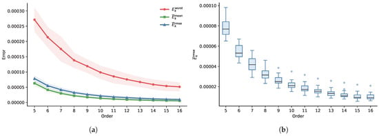
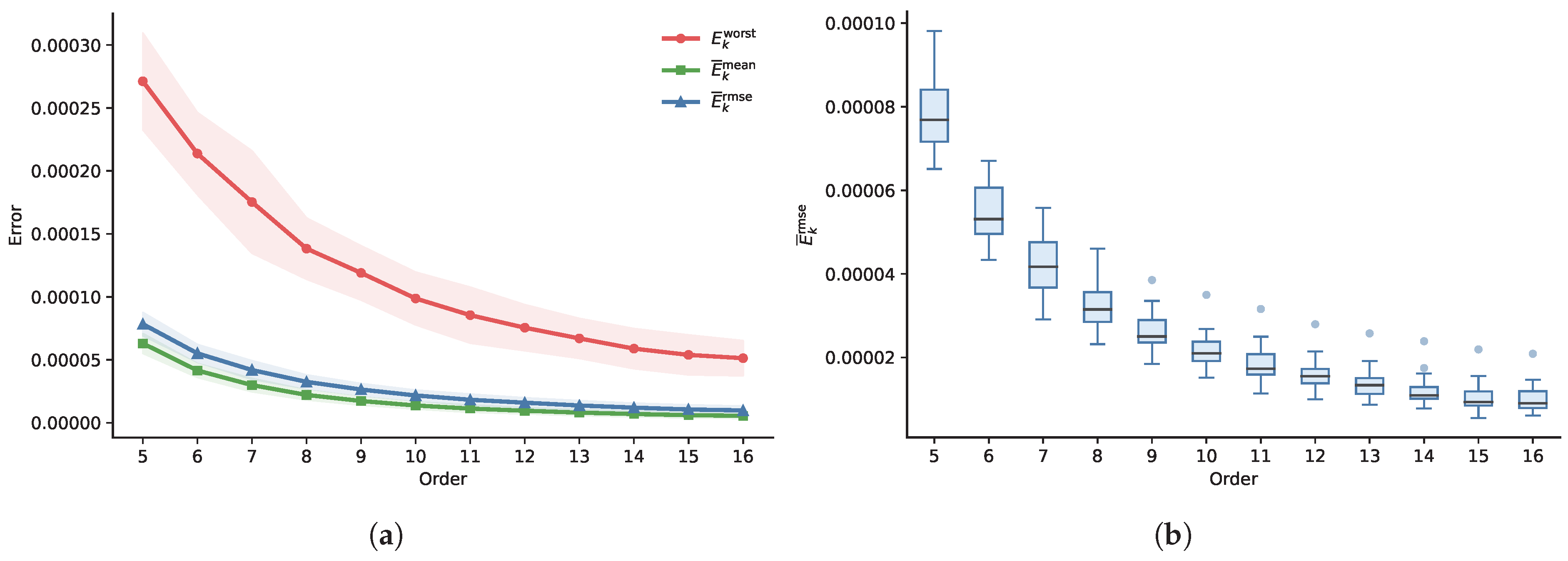
Their standard deviations are also computed and shown as shaded bands in Figure 15a. To further examine the effect of parameter scaling, we normalize the parameter domain by

$$\widehat{t}={\displaystyle \frac{t-t_{\min }}{t_{\max }-t_{\min }}},{\widehat{t}}_i={\displaystyle \frac{t_i-t_{\min }}{t_{\max }-t_{\min }}},$$

and repeat the same perturbation experiment. Let ${\overline{E}}_{k,\mathrm{raw}}^{\mathrm{rmse}}$ and ${\overline{E}}_{k,\mathrm{norm}}^{\mathrm{rmse}}$ denote the average RMSE before and after normalization, respectively. Their ratio is defined as

$$R_k={\displaystyle \frac{{\overline{E}}_{k,\mathrm{norm}}^{\mathrm{rmse}}}{{\overline{E}}_{k,\mathrm{raw}}^{\mathrm{rmse}}}}.$$

Figure 15. Numerical stability of higher-order Ball-Spline basis functions under knot perturbations. (a) Error statistics with mean and one standard deviation; (b) distribution of average basis RMSE over multiple random trials.

As shown in Figure 15a, all three error measures decrease monotonically as the order increases, indicating that higher-order Ball-Spline basis functions become less sensitive to knot perturbations. The boxplots in Figure 15b further show that the median RMSE and its spread both decrease as the order increases, demonstrating improved robustness across random trials. The quantitative results in Table 5 confirm this trend. This behavior can be attributed to the smooth polynomial representation and exact integration of each spline segment, resulting in numerical stability under knot perturbations. Moreover, Table 6 shows that $R_k\approx 1$ for all tested orders, which implies that parameter normalization has little practical effect on the stability results.

Table 5. Numerical stability of high-order Ball-Spline basis functions under knot perturbation.

Order	${\overline{\mathit{E}}}_{\mathit{k}}^{\mathbf{mean}}$	${\overline{\mathit{E}}}_{\mathit{k}}^{\mathbf{rmse}}$	${\mathit{E}}_{\mathit{k}}^{\mathbf{worst}}$
5	6.3002 $\times {10}^{-5}$	7.8346 $\times {10}^{-5}$	2.7117 $\times {10}^{-4}$
6	4.1530 $\times {10}^{-5}$	5.5132 $\times {10}^{-5}$	2.1379 $\times {10}^{-4}$
7	2.9935 $\times {10}^{-5}$	4.1874 $\times {10}^{-5}$	1.7531 $\times {10}^{-4}$
8	2.2101 $\times {10}^{-5}$	3.2502 $\times {10}^{-5}$	1.3830 $\times {10}^{-4}$
9	1.7296 $\times {10}^{-5}$	2.6398 $\times {10}^{-5}$	1.1901 $\times {10}^{-4}$
10	1.3731 $\times {10}^{-5}$	2.1697 $\times {10}^{-5}$	9.8691 $\times {10}^{-5}$
11	1.1252 $\times {10}^{-5}$	1.8263 $\times {10}^{-5}$	8.5452 $\times {10}^{-5}$
12	9.5636 $\times {10}^{-6}$	1.5941 $\times {10}^{-5}$	7.5498 $\times {10}^{-5}$
13	8.0679 $\times {10}^{-6}$	1.3720 $\times {10}^{-5}$	6.6988 $\times {10}^{-5}$
14	6.9586 $\times {10}^{-6}$	1.2014 $\times {10}^{-5}$	5.8873 $\times {10}^{-5}$
15	6.0222 $\times {10}^{-6}$	1.0563 $\times {10}^{-5}$	5.3907 $\times {10}^{-5}$
16	5.5044 $\times {10}^{-6}$	9.8216 $\times {10}^{-6}$	5.1284 $\times {10}^{-5}$

Table 6. Comparison of average basis RMSE before and after parameter normalization.

Order	${\overline{\mathit{E}}}_{\mathit{k},\mathbf{raw}}^{\mathbf{rmse}}$	${\overline{\mathit{E}}}_{\mathit{k},\mathbf{norm}}^{\mathbf{rmse}}$	${\mathit{R}}_{\mathit{k}}$
5	7.8346 $\times {10}^{-5}$	7.8346 $\times {10}^{-5}$	1.0000
6	5.5132 $\times {10}^{-5}$	5.5132 $\times {10}^{-5}$	1.0000
7	4.1874 $\times {10}^{-5}$	4.1874 $\times {10}^{-5}$	1.0000
8	3.2502 $\times {10}^{-5}$	3.2502 $\times {10}^{-5}$	1.0000
9	2.6398 $\times {10}^{-5}$	2.6398 $\times {10}^{-5}$	1.0000
10	2.1697 $\times {10}^{-5}$	2.1697 $\times {10}^{-5}$	1.0000
11	1.8263 $\times {10}^{-5}$	1.8263 $\times {10}^{-5}$	1.0000
12	1.5941 $\times {10}^{-5}$	1.5941 $\times {10}^{-5}$	1.0000
13	1.3720 $\times {10}^{-5}$	1.3720 $\times {10}^{-5}$	0.99998
14	1.2014 $\times {10}^{-5}$	1.2014 $\times {10}^{-5}$	0.99999
15	1.0563 $\times {10}^{-5}$	1.0562 $\times {10}^{-5}$	0.99990
16	9.8216 $\times {10}^{-6}$	9.8012 $\times {10}^{-6}$	0.99792

4.8. Systematic Comparison

To provide a clearer comparison, we present a comparison between Ball-Spline curves and B-spline curves in Table 7.

Table 7. Systematic comparison between Ball-Spline curves and B-spline curves.

Aspect	Ball-Spline Curve	B-Spline Curve
Construction	Generated from a spline-type extension of the Ball basis	Generated from a spline-type extension of the Bernstein basis
Curve definition	$\mathit{P}\left(t\right)={\displaystyle \sum _{i=1}^n}{B}_{i,k}\left(t\right){\mathit{P}}_{\mathit{i}}$	$\mathit{P}\left(t\right)={\displaystyle \sum _{i=1}^n}{N}_{i,k}\left(t\right){\mathit{P}}_{\mathit{i}}$
Convex hull property	Yes	Yes
Affine invariance	Yes	Yes
Local control	Yes	Yes
Continuity	$$\left\{\begin{array}{ccc}{C}^{k-3},\hfill & & l_j=1,\hfill \\ C^{k-1-l_j},\hfill & & l_j\ge 2.\hfill \end{array}\right.$$ $l_j$: multiplicity of knot $t_j$ (see Proposition 18)	$C^{k-1-l_j}$, $l_j$: multiplicity of knot $t_j$
Degeneracy	Reduces to the classical cubic Ball curve	Reduces to the Bézier curve
Computational cost	Higher in practice (see Section 4.6)	Lower
Numerical stability	Stable under knot perturbations (see Section 4.7)	Numerical stability ensured by the de Boor-Cox recursion
Control point efficiency	Fewer control points for in some cases (see Section 4.5)	Standard

5. Conclusions

This paper presents a construction of spline-type Ball basis functions, demonstrates the existence of such basis functions with the highest order of continuity, and proves that they possess the fundamental properties, thereby achieving a valid theoretical generalization. The proposed Ball-Spline basis functions can generate design curves with fewer control points under the same approximation accuracy and parameter interval partition. However, the proposed fourth-order basis functions involve relatively complicated representations and do not possess properties analogous to the knot insertion property and the de Boor–Cox recursive algorithm of B-splines. Future work may consider appropriately relaxing the continuity conditions to simplify the basis function expressions, and investigate efficient recursive schemes and knot insertion mechanisms, with the aim of further strengthening the theoretical framework.

References

- Gordon, W.J.; Riesenfeld, R.F. B-spline curves and surfaces. Comput. Aided Geom. Des. 1974, 1, 95–126. [Google Scholar]
- Biswas, S.; Lovell, B.C. Bernstein Polynomial and Bézier-Bernstein Spline. In Bézier and Splines in Image Processing and Machine Vision; Springer: Berlin/Heidelberg, Germany, 2008; pp. 3–32. [Google Scholar]
- Chudy, F.; Woźny, P. Linear-time algorithm for computing the Bernstein–Bézier coefficients of B-spline basis functions. Comput.-Aided Des. 2023, 154, 103434. [Google Scholar] [CrossRef] [Scilit]
- Versprille, K.J. Computer-Aided Design Applications of the Rational B-Spline Approximation Form. Ph.D. Dissertation, Syracuse University, Syracuse, NY, USA, 1975. [Google Scholar]
- Uhm, T.K.; Youn, S.K. T-spline finite element method for the analysis of shell structures. Int. J. Numer. Methods Eng. 2009, 80, 507–536. [Google Scholar] [CrossRef] [Scilit]
- Li, M.; Shen, W. Integral method from even to odd order for trigonometric B-spline basis. AIMS Math. 2024, 9, 36470–36492. [Google Scholar] [CrossRef] [Scilit]
- Khater, M.M.; Ahmed, A.E.-S. Strong Langmuir turbulence dynamics through the trigonometric quintic and exponential B-spline schemes. AIMS Math. 2021, 6, 5896–5908. [Google Scholar] [CrossRef] [Scilit]
- Majeed, A.; Abbas, M.; Sittar, A.A.; Misro, M.Y.; Kamran, M. Airplane designing using Quadratic Trigonometric B-spline with shape parameters. AIMS Math. 2021, 6, 7669–7683. [Google Scholar] [CrossRef] [Scilit]
- Shen, W.; Wang, G. Changeable degree spline basis functions. J. Comput. Appl. Math. 2010, 234, 2516–2529. [Google Scholar] [CrossRef] [Scilit]
- Toshniwal, D.; Speleers, H.; Hiemstra, R.R.; Manni, C.; Hughes, T.J.R. Multi-degree B-splines: Algorithmic computation and properties. Comput. Aided Geom. Des. 2020, 76, 101792. [Google Scholar] [CrossRef] [Scilit]
- Hiemstra, R.R.; Hughes, T.J.R.; Manni, C.; Speleers, H.; Toshniwal, D. A Tchebycheffian extension of multi-degree B-splines: Algorithmic computation and properties. SIAM J. Numer. Anal. 2020, 58, 1138–1163. [Google Scholar] [CrossRef] [Scilit]
- Speleers, H. Algorithm 1020: Computation of multi-degree Tchebycheffian B-splines. ACM Trans. Math. Softw. 2022, 48, 1–31. [Google Scholar] [CrossRef] [Scilit]
- Manni, C.; Pelosi, F.; Sampoli, M.L. Generalized B-splines as a tool in isogeometric analysis. Comput. Methods Appl. Mech. Eng. 2011, 200, 867–881. [Google Scholar] [CrossRef] [Scilit]
- Vivas-Cortez, M.; Yousif, M.A.; Mahmood, B.A.; Mohammed, P.O.; Chorfi, N.; Lupas, A.A. High-accuracy solutions to the time-fractional KdV–Burgers equation using rational non-polynomial splines. Symmetry 2025, 17, 16. [Google Scholar] [CrossRef] [Scilit]
- Vivas-Cortez, M.; Yousif, M.A.; Mohammed, P.O.; Chorfi, N.; Lupas, A.A. Hyperbolic non-polynomial spline approach for time-fractional coupled KdV equations: A computational investigation. Symmetry 2024, 16, 1610. [Google Scholar] [CrossRef] [Scilit]
- Yousif, M.A.; Agarwal, R.P.; Mohammed, P.O.; Chorfi, N.; Lupas, A.A. Advanced methods for conformable time-fractional differential equations: Logarithmic non-polynomial splines. Axioms 2024, 13, 551. [Google Scholar] [CrossRef] [Scilit]
- Meetei, M.Z.; Tamsir, M.; Singh, M.; Dhiman, N.; Khan, F.A. A new uniform hyperbolic polynomial B-spline computational scheme for 3rd-order pseudo-parabolic problem. Mathematics 2026, 14, 542. [Google Scholar] [CrossRef] [Scilit]
- Ball, A.A. CONSURF. Part 1: Introduction to the conic lofting title. Comput.-Aided Des. 1974, 6, 243–249. [Google Scholar] [CrossRef] [Scilit]
- Ball, A.A. CONSURF. Part two: Description of the algorithms. Comput.-Aided Des. 1975, 7, 237–242. [Google Scholar] [CrossRef] [Scilit]
- Ball, A.A. CONSURF. Part 3: How the program is used. Comput.-Aided Des. 1977, 9, 9–12. [Google Scholar] [CrossRef] [Scilit]
- Wang, G.J. Ball curve of high degree and its geometric properties. Appl. Math. J. Chin. Univ. 1987, 2, 126–140. [Google Scholar]
- Said, H.B. A generalized Ball curve and its recursive algorithm. ACM Trans. Graph. 1989, 8, 360–371. [Google Scholar] [CrossRef] [Scilit]
- Goodman, T.N.T.; Said, H.B. Properties of generalized Ball curves and surfaces. Comput.-Aided Des. 1991, 23, 554–560. [Google Scholar] [CrossRef] [Scilit]
- Goodman, T.N.T.; Said, H.B. Shape preserving properties of the generalised Ball basis. Comput. Aided Geom. Des. 1991, 8, 115–121. [Google Scholar] [CrossRef] [Scilit]
- Hu, S.-M.; Wang, G.-Z.; Jin, T.-G. Properties of two types of generalized Ball curves. Comput.-Aided Des. 1996, 28, 125–133. [Google Scholar] [CrossRef] [Scilit]
- Othman, W.A.M.; Goldman, R.N. The dual basis functions for the generalized Ball basis of odd degree. Comput. Aided Geom. Des. 1997, 14, 571–582. [Google Scholar] [CrossRef] [Scilit]
- Delgado, J.; Peña, J.M. A linear complexity algorithm for the Bernstein basis. In Proceedings of the International Conference on Geometric Modeling and Graphics, London, UK, 16–18 July 2003; pp. 162–167. [Google Scholar]
- Hu, Q.-Q.; Wang, G.-J. Rational cubic/quartic Said-Ball conics. Appl. Math. J. Chin. Univ. 2011, 26, 198–212. [Google Scholar] [CrossRef] [Scilit]
- Yan, L.; Wu, G.; Liang, J. Generalized Ball curves of ninth degree. In Proceedings of the International Conference on Environmental Science and Information Application Technology, Wuhan, China, 4–5 July 2009; pp. 557–560. [Google Scholar]
- Wu, X.-Q.; Han, X.-L. Shape analysis of quartic Ball curve with shape parameter. Acta Math. Appl. Sin. 2011, 34, 671–682. [Google Scholar]
- Liu, H.-Y.; Li, L.; Zhang, D.-M. Quadratic Ball curve with multiple shape parameters. Shandong Daxue Xuebao (Eng. Sci.) 2011, 41, 23–28. [Google Scholar]
- Huang, C.-L.; Huang, Y.-D. Quartic Wang-Ball type curves and surfaces with two parameters. J. Hefei Univ. Technol. 2012, 35, 1436–1440. [Google Scholar]
- Wang, C.-W.; Chen, H. Extension of quartic Said-Ball curve with two parameters. In Mechanics and Mechanical Engineering; 2016; pp. 543–552. Available online: https://www.worldscientific.com/doi/pdf/10.1142/9789813145603_0066?srsltid=AfmBOorN30Fk056WBdBVWCgBTphs7kKK8AoQHC6dzy6i_Bi1QDkWlaS_ (accessed on 25 March 2026).
- Hu, G.; Luo, L.; Li, R.; Yang, C. Quartic generalized Ball surfaces with shape parameters and its continuity conditions. In Proceedings of the International Conference on Computer Science and Network Technology, Dalian, China, 21–22 October 2017; pp. 5–10. [Google Scholar]
- Hu, G.; Du, B. Ball Said-Ball curve: Construction and its geometric algorithms. Adv. Eng. Softw. 2022, 174, 103334. [Google Scholar] [CrossRef] [Scilit]
- Hu, G.; Zhu, X.; Wei, G.; Chang, C.-T. An improved marine predators algorithm for shape optimization of developable Ball surfaces. Eng. Appl. Artif. Intell. 2021, 105, 104417. [Google Scholar] [CrossRef] [Scilit]
- Hu, G.; Li, M.; Wang, X.; Wei, G.; Chang, C.-T. An enhanced manta ray foraging optimization algorithm for shape optimization of complex CCG-Ball curves. Knowl.-Based Syst. 2022, 240, 108071. [Google Scholar] [CrossRef] [Scilit]
- Du, B.; Yuan, X.; Zhong, J.; Hu, G. Construction of Generalized λμ-Ball Curves of Degree n. In Proceedings of the International Conference on Image, Vision and Computing, Xi’an, China, 26–28 July 2022; pp. 498–501. [Google Scholar]
- Zheng, J.; Ji, X.; Ma, Z.; Hu, G. Construction of local-shape-controlled quartic generalized Said-Ball model. Mathematics 2023, 11, 2369. [Google Scholar] [CrossRef] [Scilit]
Disclaimer/Publisher’s Note: The statements, opinions and data contained in all publications are solely those of the individual author(s) and contributor(s) and not of MDPI and/or the editor(s). MDPI and/or the editor(s) disclaim responsibility for any injury to people or property resulting from any ideas, methods, instructions or products referred to in the content. |
© 2026 by the authors. Licensee MDPI, Basel, Switzerland. This article is an open access article distributed under the terms and conditions of the Creative Commons Attribution (CC BY) license.