Causal-Enhanced Spatio-Temporal Markov Graph Convolutional Network for Traffic Flow Prediction

Abstract

Traffic flow prediction is a pivotal task in intelligent transportation systems. The primary challenge lies in accurately modeling the dynamically evolving and directional spatio-temporal dependencies inherent in road networks. Existing graph neural network-based methods suffer from three main limitations: (1) symmetric adjacency matrices fail to capture the causal propagation of traffic flow from upstream to downstream; (2) the serial combination of graph and temporal convolutions lacks an explicit modeling of joint spatio-temporal state transition probabilities; (3) the inherent low-pass filtering property of temporal convolutional networks tends to smooth high-frequency abrupt signals, thereby weakening responsiveness to sudden events. To address these issues, this paper proposes a causal-enhanced spatio-temporal Markov graph convolutional network (CSHGCN). At the spatial modeling level, we construct an asymmetric causal adjacency matrix by decoupling source and target node embeddings to learn directional traffic flow influences. At the spatio-temporal joint modeling level, we design a spatio-temporal Markov transition module (STMTM) based on spatio-temporal Markov chain theory, which explicitly learns conditional transition patterns through temporal dependency encoders, spatial dependency encoders, and a joint transition network. At the temporal modeling level, we introduce differential feature enhancement and high-frequency residual compensation mechanisms to preserve key abrupt change information through frequency-domain complementarity. Experiments on four datasets—PEMS03, PEMS04, PEMS07, and PEMS08—demonstrate that CSHGCN outperforms existing baselines in terms of MAE, RMSE, and MAPE, with ablation studies validating the effectiveness of each module.

1. Introduction

Intelligent transportation systems (ITS) serve as the core supporting technology for modern urban governance and transportation management. By enabling real-time traffic data collection, intelligent analysis, and decision optimization, ITS significantly enhance traffic operational efficiency, reduce energy consumption, and mitigate environmental emissions. They play a vital role in alleviating urban congestion and improving travel experience [1]. Traffic state prediction aims to forecast traffic flow conditions within specific future time windows based on historical observation data, serving as the data foundation for applications such as traffic signal control [2], emergency incident response [3], and travel route planning [4] in ITS. As urban road networks expand and data collection frequency increases, traffic flow data exhibit high-dimensional and non-stationary characteristics. Consequently, traditional statistical methods like ARIMA [5] struggle to capture long-term temporal dependencies and nonlinear spatial correlations effectively. In recent years, hybrid architectures integrating graph convolutional networks (GCN) [6] and temporal convolutional networks (TCN) [7] have become mainstream. GCN models spatial dependencies among road network nodes via adjacency matrices, while TCN extracts long-term temporal features through dilated convolutions.

However, facing the complex dynamic characteristics of real traffic systems, existing methods exhibit deficiencies in the following three modeling aspects: (1) Lack of Spatial Causality: Most methods employ symmetric adjacency matrices or undirected graphs, which fail to capture the asymmetric causal propagation inherent in traffic flow, thereby limiting prediction accuracy. (2) Weakness in Spatio-Temporal Joint Modeling: The evolution of traffic states across time and space dimensions is not independent but tightly coupled. Current mainstream architectures combine spatio-temporal features in serial or parallel manners using GNN and TCN, lacking explicit modeling of the probability of future states given historical spatio-temporal conditions, making it difficult to formally capture state transition patterns. (3) Loss of Temporal High-Frequency Information: TCN possesses low-pass filtering characteristics that systematically attenuate high-frequency components.

Therefore, this paper proposes a causality-enhanced spatio-temporal Markov graph convolutional network, aiming to achieve systematic innovation at the model architecture level. The core motivations of this work are: (1) to explicitly model the physical propagation direction of traffic flow from upstream to downstream by constructing an asymmetric causal adjacency matrix; (2) to introduce the mathematical framework of spatio-temporal Markov chains and design a learnable joint transition module, which characterizes the co-evolution of spatio-temporal states in the form of explicit conditional probabilities; and (3) from the perspective of frequency-domain analysis, to design complementary input enhancement and output compensation mechanisms to counteract the inherent smoothing effect of temporal convolutions. These three aspects are closely interlinked, collectively forming a deep learning framework that better aligns with the physical nature and data characteristics of transportation systems. The main contributions of this paper are as follows:

1. We introduce a causal-enhanced adjacency matrix construction method. By separately learning node embeddings as information senders and receivers, we generate an asymmetric adjacency matrix to model directional spatial dependencies in traffic flow.

2. We design a spatio-temporal Markov transition module (STMTM), integrating the probabilistic framework of spatio-temporal Markov chains into deep networks. This module explicitly learns conditional transition patterns across spatio-temporal dimensions through temporal dependency encoders, spatial dependency encoders, and a joint transition network.

3. We propose a high-frequency-aware temporal enhancement strategy. Differential feature enhancement introduces high-frequency change information at the input, while high-frequency residual compensation corrects the smoothing effect of TCN at the output, achieving frequency-domain complementarity.

4. We conduct extensive experiments on four public datasets, demonstrating that CSHGCN outperforms existing methods in prediction accuracy. Ablation studies further confirm the contributions of each module.

The remainder of this paper is organized as follows. Section 2 systematically reviews related work in the field of traffic prediction. Section 3 introduces necessary preliminaries, including problem definition and theoretical foundations. Section 4 elaborates on the overall framework and core module designs of CSHGCN. Section 5 describes the experimental setup, including datasets, evaluation metrics, and baseline methods. Section 6 presents the experimental results, with comprehensive performance comparison, ablation studies, and visual analysis. Section 7 provides an in-depth discussion on the design advantages and synergistic relationships of each module. Section 8 concludes the paper and outlines future research directions.

2. Related Work

Traffic flow prediction, as a core technology for dynamic road network control and travel scheduling, has long received widespread attention from both academia and industry. Its essence belongs to spatio-temporal sequence forecasting, with the core challenge being how to effectively model dynamically evolving spatio-temporal dependencies within road networks. Early research primarily employed traditional statistical methods, such as autoregressive integrated moving average (ARIMA) [5] and vector autoregression (VAR) [8], which are based on classical time series analysis principles [9]. Although these methods are effective in certain scenarios, their modeling capabilities are limited by stationarity assumptions [10], making it difficult to characterize nonlinear features in traffic data. More importantly, they typically process each road segment’s time series data independently, ignoring spatial correlations among nodes in the road network, thus yielding limited prediction performance in real-world complex road networks.

With the development of deep learning, deep neural networks (DNNs) [11] have been gradually introduced into the traffic prediction domain, significantly enhancing model ability to extract spatio-temporal features. For instance, fully connected long short-term memory networks (FC-LSTM) [12] model time series data by integrating convolutional and recurrent structures; spatio-temporal residual networks (ST-ResNet) [13] utilize deep residual convolutional networks to predict urban crowd flows, demonstrating powerful feature representation capabilities. However, these methods are primarily designed for grid-based or sequential data, without explicitly leveraging the topological structure of road networks, and thus still exhibit suboptimal performance on graph-structured traffic data.

To effectively incorporate road network structure information, graph convolutional networks (GCNs) [14] have been introduced into traffic prediction, explicitly modeling spatial dependencies through adjacency matrices. Early works such as STGCN [15] and DCRNN [16] relied on pre-defined adjacency matrices, making it difficult to reflect dynamic and asymmetric spatial relationships. Foundational work in GCN, such as GraphSAGE [17], laid the groundwork for learning representations on graph-structured data. Subsequently, research shifted toward adaptive graph learning; for example, Graph WaveNet [18] and MTGNN [19] dynamically generate adjacency matrices by learning node embeddings, while AGCRN [20] learns independent embeddings for each node to capture node-specific patterns.

Simultaneously, methods based on attention mechanisms have moved away from reliance on pre-defined graph structures, dynamically modeling global dependencies by computing the similarity weights between elements. This trend has been significantly influenced by the Transformer [21] architecture proposed by Vaswani et al., which revolutionized sequence modeling. Models such as ASTGCN [22], GMAN [23] successfully capture long-range spatio-temporal correlations; subsequent works like Informer [24], Autoformer [25], and FEDformer [26] further enhance model efficiency and performance from perspectives such as sparse attention, sequence decomposition, and frequency-domain enhancement. Furthermore, the Graph Attention Network (GAT) [27] a pioneering framework for directly applying attention mechanisms to graphs.

In recent years, to enhance model interpretability and dynamic modeling capabilities, researchers have begun exploring methods that combine explicit structure learning with joint state modeling. For instance, STG-NCDE [28] integrates adaptive graphs with neural controlled differential equations to characterize traffic evolution in continuous time domains; spatio-temporal graph diffusion networks (ST-GDN) [29] and dynamic spatio-temporal aware graph neural networks (DSTAGNN) [30] dynamically capture changes in inter-node relationships by directly mining spatio-temporal patterns from historical data. Moreover, to handle uncertainty and dynamics in traffic systems, some studies have begun incorporating probabilistic graphical models. For example, Peng et al. [31] proposed a reinforcement learning-based dynamic graph generation framework that optimizes graph structures through interactive learning to extract more interpretable spatio-temporal features. Beyond transportation research, the integration of causal inference and machine learning has gained increasing attention for building more robust and interpretable models. Theoretical foundations in machine learning causality [32], along with subsequent explorations of causal representation on graphs [33], offer a principled perspective beyond mere correlation, inspiring our approach to modeling directional dependencies. In the field of traffic prediction, some studies attempt to uncover potential causal structures among nodes in road networks using Granger causality tests, structural causal models, or intervention-based reasoning, and then incorporate these as constraints or prior knowledge into graph neural networks.

Although the aforementioned methods have achieved accurate predictions, they still possess several shortcomings. Firstly, the learned spatial relationships often lack clear physical or causal explanations, making it difficult to reflect the directional influence of traffic flow. Alternatively, they focus on “causal discovery,” a process typically independent of the prediction task and characterized by high computational complexity; Second, spatio-temporal features are processed in serial or parallel manners, resulting in insufficiently tight spatio-temporal coupling. Finally, while temporal dilated convolution methods are effective, they tend to excessively smooth traffic flow time series, leading to the neglect of crucial high-frequency information.

3. Preliminaries

3.1. Problem Definition of Spatio-Temporal Traffic Flow

Definition 1 

(Traffic Network Graph). A traffic network can be represented as a directed graph $G=(V,\mathcal{E},A)$, where V denotes the set of nodes with $\left|V\right|=N$ representing the number of traffic sensors; $\mathcal{E}$ is the edge set, denoting connectivity relationships between road segments; and $A\in {\mathbb{R}}^{N\times N}$ is the adjacency matrix that characterizes the spatial dependency strength between nodes.

Definition 2 

(Traffic Flow Sequence). A traffic flow sequence is represented as $\mathcal{X}\in {\mathbb{R}}^{N\times T\times C}$, where N is the number of nodes, T is the number of time steps, and C is the feature dimension.

Definition 3 

(Traffic Flow Prediction Problem). Given a historical traffic observation sequence of $T_h$ time steps $X_{t-T_h+1:t}=[X_{t-T_h+1},\dots ,X_t]$, the goal is to predict the future $T_f$ time steps of traffic state sequence $Y_{t+1:t+T_f}=[X_{t+1},\dots ,X_{t+T_f}]$. This problem can be formalized as learning a mapping function $\mathcal{F}:(X_{t-T_h+1:t},G)\to Y_{t+1:t+T_f}$.

3.2. Graph WaveNet Model

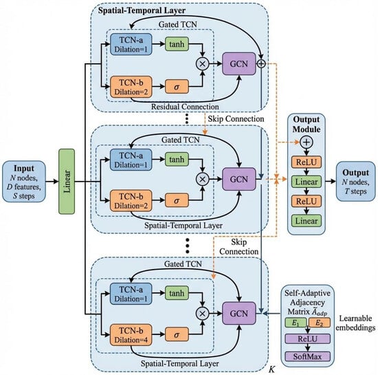
Wu et al. [18] proposed Graph WaveNet (GWNET), a novel graph neural network architecture for spatio-temporal graph modeling. It learns an adaptive dependency matrix through node embeddings, enabling hidden spatial dependencies in the data to be captured. By stacking dilated convolutions, the model’s receptive field expands exponentially with depth, allowing it to handle very long sequences. GWNET is composed of multiple stacked spatio-temporal layers, each containing a graph convolutional layer (GCN) and a gated temporal convolutional layer (Gated TCN), followed by an output layer that directly produces multi-step predictions.

In the graph convolutional layer (GCN), the adaptive adjacency matrix is automatically learned from node embeddings. It is defined as follows:

$$A_{adp}=\mathrm{SoftMax}\left(\mathrm{ReLU}\left(E_1{E}_2^T\right)\right)$$

(1)

where $E_1,E_2\in {\mathbb{R}}^{N\times c}$ are learnable node embeddings, computing dependency strength between nodes via the inner product, with ReLU filtering weak connections and SoftMax performing normalization. Predefined forward and backward diffusion convolutions are combined with the adaptive adjacency matrix, as shown in Equation (2):

$$\mathcal{Z}=\sum _{k=0}^K\left(P_f^k{\mathbf{W}}_{k1}+P_b^k{\mathbf{W}}_{k2}+A_{adp}{\mathbf{W}}_{k3}\right)$$

(2)

If the graph structure is unknown, only the adaptive part is used, as in Equation (3):

$$\mathcal{Z}=\sum _{k=0}^K{A}_{adp}{\mathbf{W}}_k$$

(3)

The temporal convolutional layer (TCN) employs dilated causal convolution to exponentially expand the receptive field with increasing layers, effectively capturing long-term temporal dependencies:

$$\mathbf{x}\star \mathbf{f}\left(t\right)=\sum _{s=0}^{K-1}\mathbf{f}\left(s\right)·\mathbf{x}(t-d\times s)$$

(4)

where d is the dilation factor controlling the skip interval. Additionally, a gating mechanism (gated TCN) is incorporated to control information flow and enhance expressive power:

$$\mathbf{h}=g({\Theta }_1\star \mathcal{X}+\mathbf{b})\odot \sigma ({\Theta }_2\star \mathcal{X}+\mathbf{c})$$

(5)

where ⊙ denotes element-wise multiplication, g is the activation function (e.g., tanh), and $\sigma$ is the sigmoid function controlling information passage ratio.

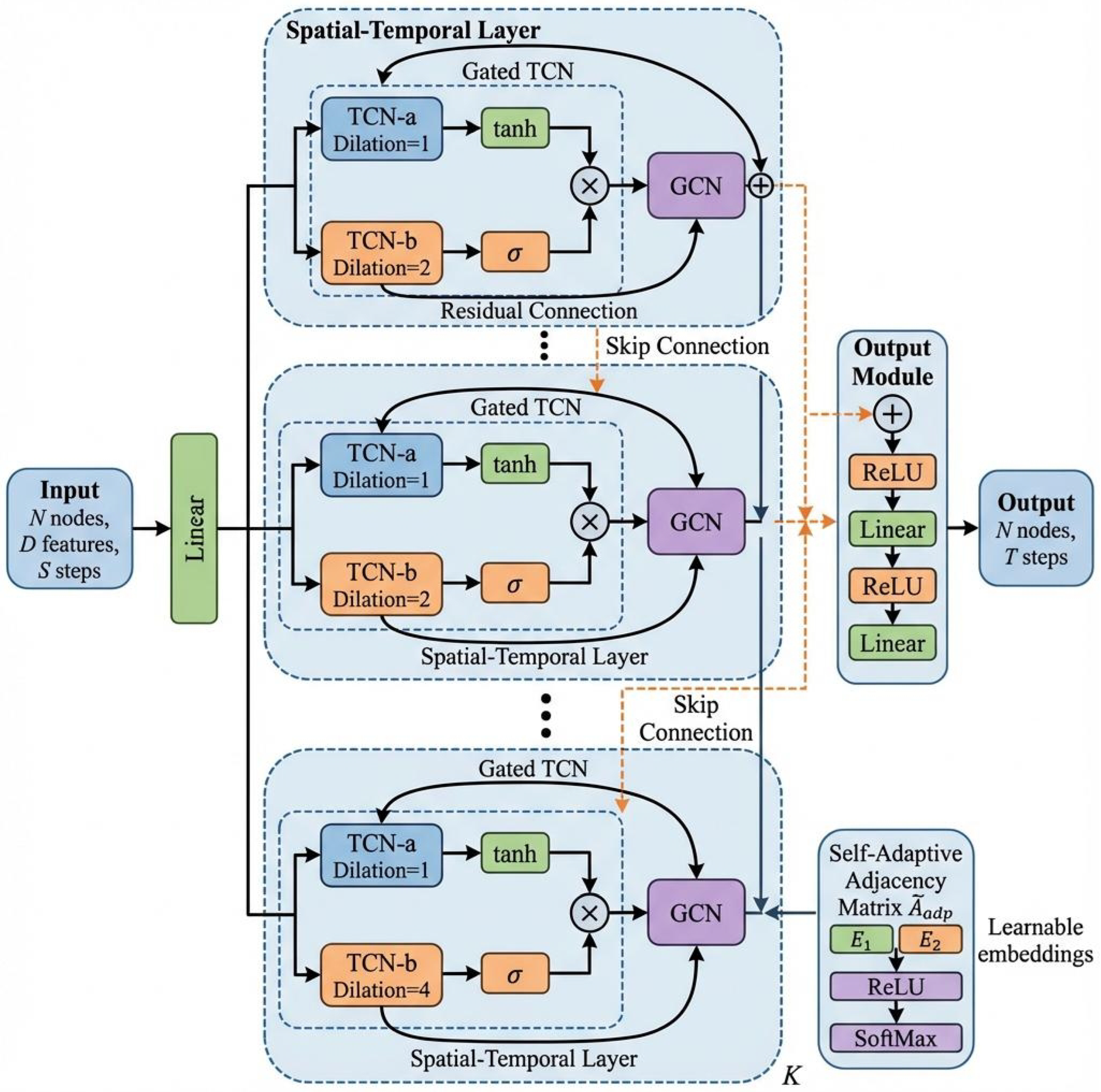
The overall framework of GWNET is shown in Figure 1, with the input being historical S-step graph signals $X^{(t-S):t}\in {\mathbb{R}}^{N\times D\times S}$. After passing through multiple spatio-temporal layers, each layer’s GCN processes features extracted by TCN at different temporal granularities. The final layer adjusts the output dimension to the prediction step T, directly outputting $X^{(t+1):(t+T)}\in {\mathbb{R}}^{N\times D\times T}$. The symbol “×” denotes dilated causal convolution, and “+” denotes element-wise addition or skip connection.

Figure 1. The overall framework of Graph WaveNet.

3.3. Theoretical Foundation

3.3.1. Mathematical Definition of Spatio-Temporal Markov Chain

We first review the mathematical definition of spatio-temporal Markov chains (STMC). Let $X_{n,m}$ be a stochastic process defined on the composite domain $\mathcal{T}\times \mathcal{S}$, where $\mathcal{T}=t_0,t_1,\dots ,t_n,\dots$ is the time domain and $\mathcal{S}=s_0,s_1,\dots ,s_m,\dots$ is the space domain.$X_{n,m}$ denotes the random variable at time index n and space index m.

According to the definition in literature [34], a spatio-temporal Markov process (STMP) satisfies the following conditional probability decomposition:

$$P\left(X_{n,m}\right|X_{n-1,m},X_{n,m-1},X_{n-1,m})=P\left(X_{n,m}\right|X_{n-1,m},X_{n,m-1})$$

(6)

This definition indicates that given the temporal predecessor $X_{n-1,m}$ and spatial predecessor $X_{n,m-1}$, the current state $X_{n,m}$ is conditionally independent of earlier historical states. This property is referred to as spatio-temporal Markovianity.

Definition 4 

(Temporal Dependence, TD). The conditional probability considering only the temporal dimension is obtained by marginalizing over the spatial variable:

$$P_{\mathcal{T}}\left(X_{n,m}\right|X_{n-1,m})=\sum _{X_{n,m}\in \sum }P\left(X_{n,m}\right|X_{n-1,m},X_{n,m-1})P\left(X_{n,m-1}\right|X_{n-1,m})$$

(7)

where ∑ is the state space. This represents the dependence of the current state on its temporal predecessor when spatial dependencies are ignored.

Definition 5 

(Spatial Dependence, SD). The conditional probability considering only the spatial dimension is obtained by marginalizing over the temporal variable:

$$P_{\mathcal{S}}\left(X_{n,m}\right|X_{n,m-1})=\sum _{X_{n,m}\in \sum }P\left(X_{n,m}\right|X_{n-1,m},X_{n,m-1})P\left(X_{n-1,m}\right|X_{n,m-1})$$

(8)

This represents the dependence of the current state on its spatial neighbors when temporal dependencies are ignored.

Definition 6 

(Spatio-temporal Joint Dependence, STD). The joint conditional probability simultaneously considering both dimensions is defined as follows:

$$P_{\mathcal{ST}}(X_{n,m}\mid X_{n-1,m},X_{n,m-1})$$

(9)

which directly models the complete dependency of the current state on both its temporal predecessor and spatial neighbors.

3.3.2. Stochastic Learning Weak Estimator (SLWE)

The stochastic learning weak estimator [35] (SLWE) can perform online incremental parameter estimation. The core update rule of SLWE is as shown in Equation (10):

$${\widehat{P}}_{s_i|s_j,s_k}^{(l+1)}=\left\{\begin{array}{cc}{\widehat{P}}_{s_i|s_j,s_k}^{\left(l\right)}+(1-\lambda ){\sum }_{r\ne i}{\widehat{P}}_{s_r|s_j,s_k}^{\left(l\right)},\hfill & \mathrm{if}{X}_{n,m}=i,X_{n-1,m}=j,X_{n,m-1}=k\hfill \\ \lambda {\widehat{P}}_{s_i|s_j,s_k}^{\left(l\right)},\hfill & \mathrm{if}{X}_{n,m}\ne i,X_{n-1,m}=j,X_{n,m-1}=k\hfill \\ {\widehat{P}}_{s_i|s_j,s_k}^{\left(l\right)},\hfill & \mathrm{if}{X}_{n-1,m}\ne j\mathrm{or}{X}_{n,m-1}\ne k\hfill \end{array}\right.$$

(10)

where $\lambda \in (0,1)$ is the learning coefficient, controlling the trade-off between old and new information. This update rule has the following characteristics:

-

When transition $(s_j,s_k)\to s_i$ is observed, increase the corresponding transition probability estimate.

-

When a transition from $(s_j,s_k)$ is observed but does not reach $s_i$, decay the corresponding transition probability estimate.

-

When observations are unrelated to the current conditional state, keep the estimate unchanged.

4. Proposed Method

4.1. CSHGCN Framework

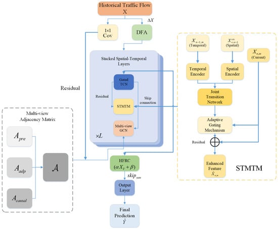
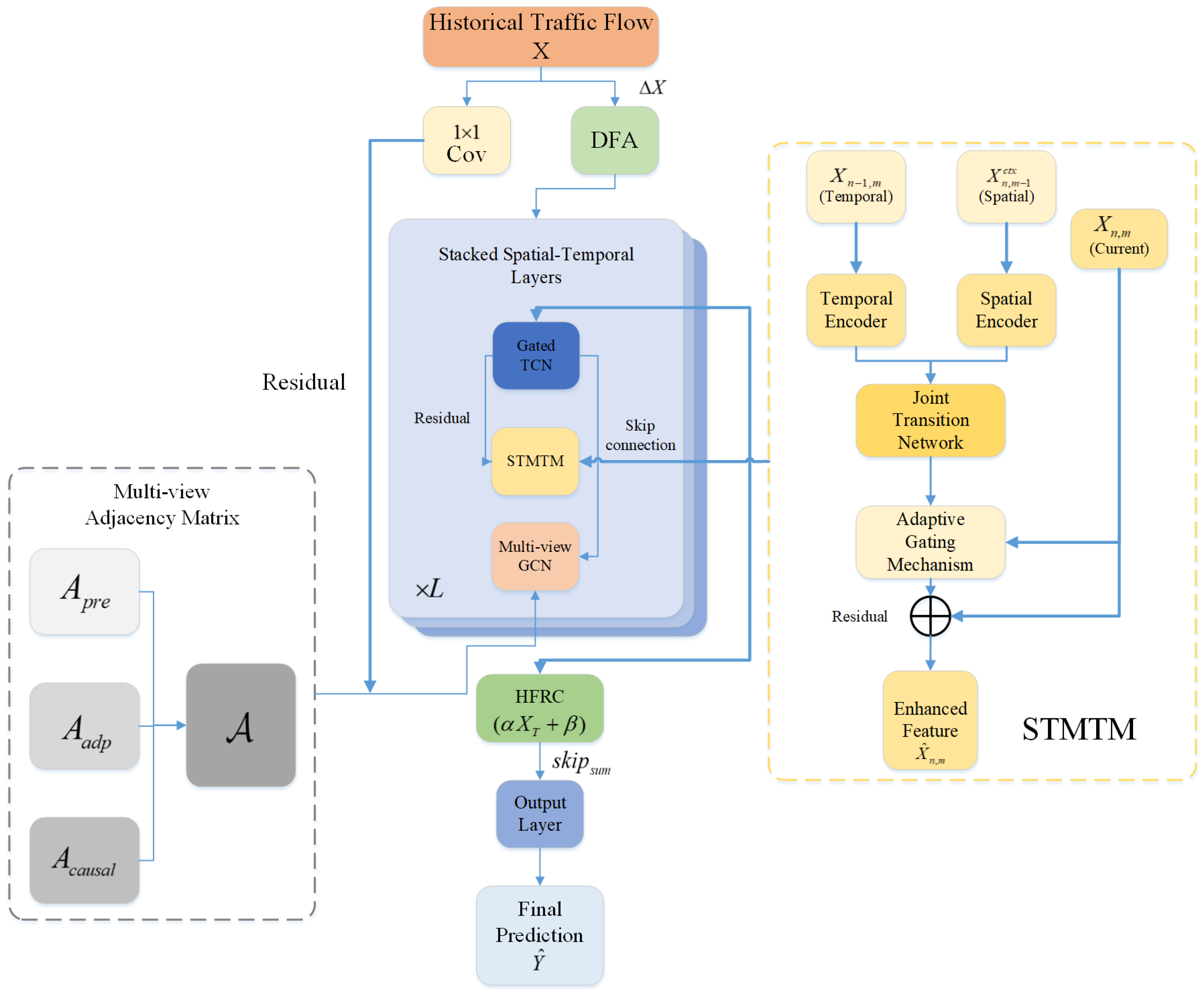
Figure 2 illustrates the framework of our proposed CSHGCN, The symbol “+” denotes element-wise addition or skip connection. Our CSHGCN improves upon the GWNET architecture. Our CSHGCN improves upon the GWNET architecture. The model takes historical traffic flow sequences as input, where the Conv_1×1 operation represents a linear transformation layer across feature dimensions, used to adjust the number of feature channels. It then sequentially performs spatial dependency extraction through causal graph convolution, models state evolution via the spatio-temporal Markov transition module, and finally outputs multi-step traffic flow predictions through temporal convolution and high-frequency-aware feature enhancement mechanisms. The forward propagation process of CSHGCN is detailed in Algorithm 1. The model details are described as follows:

Figure 2. The overall framework of CSHGCN.

Causal-Enhanced Graph Structure Learning: This module constructs a learnable adjacency matrix that explicitly reflects the upstream-to-downstream propagation direction of traffic flow. The learned causal matrix is combined with a predefined adjacency matrix (based on physical road connectivity) and a fully data-driven adaptive adjacency matrix. This multi-view aggregation provides a more realistic characterization of directional influences within the traffic network.

Spatio-Temporal Markov Transition Module (STMTM): This module contains a temporal dependency encoder, a spatial dependency encoder, and a spatio-temporal joint transition network. By jointly encoding the state at historical moments and the state of spatial neighborhoods, it explicitly learns the conditional transition patterns of traffic states across spatio-temporal dimensions. Additionally, the module incorporates an adaptive gating mechanism that dynamically adjusts information fusion intensity based on current traffic conditions, enhancing the model’s adaptability to non-stationary traffic pattern changes.

High-Frequency-Aware Temporal Enhancement Module: This module includes differential feature enhancement and high-frequency residual compensation mechanisms. Differential feature enhancement highlights traffic flow abrupt change events by introducing first-order differential information of traffic flow into the input; high-frequency residual compensation adaptively corrects the model output based on the last observed value to restore smoothed key high-frequency details.

4.2. Causal-Enhanced Adaptive Adjacency Matrix

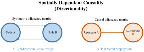
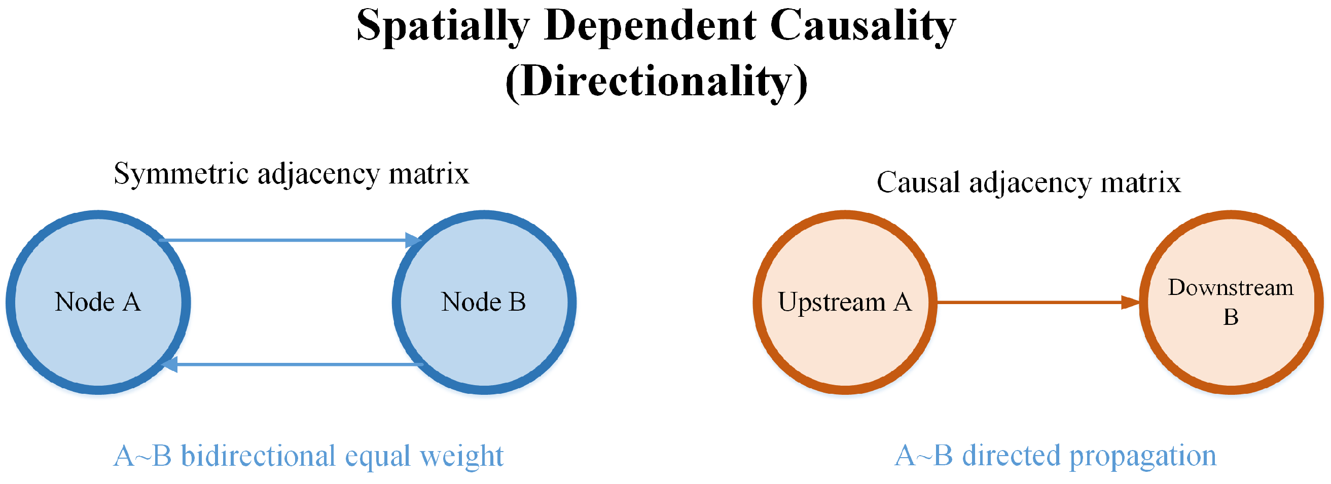
According to structural causal model (SCM) theory [36], the core characteristic distinguishing causality from general statistical correlation lies in the directionality of intervention effects. Interventions on cause variables affect outcome variables, while interventions on outcome variables do not inversely affect cause variables. This causal characteristic is particularly evident in traffic scenarios, as shown in Figure 3. However, graph neural network models, exemplified by Graph WaveNet, mostly employ symmetric adjacency matrices for spatial modeling. This symmetry assumption essentially reduces the causal dependency between nodes to a bidirectional, equal-strength statistical correlation, failing to capture the causal mechanism in traffic flow propagation. To address this issue, this paper proposes a causality-enhanced adaptive adjacency matrix construction method, which learns an asymmetric adjacency matrix that reflects the causal structure of the traffic network. Instead of striving to learn the complete causal graph from data, we explicitly model the inherent, directional causal prior of traffic flow propagating from upstream to downstream by decoupling node embeddings. This paradigm focuses more on effectively encoding known causal commonsense into the model to improve prediction performance and directional interpretability, achieving an efficient balance between complexity and effectiveness.

Algorithm 1 CSHGCN Forward Propagation

Require: Historical traffic flow sequence $X\in {\mathbb{R}}^{B\times C\times N\times T}$

Ensure: Prediction result $Y_{final}\in {\mathbb{R}}^{B\times T_f\times N\times 1}$

1:  // — Phase 1: Input processing and graph structure construction —    2:  $\Delta X\leftarrow \mathrm{Diff}\left(X\right)$                ▹ Calculate first-order temporal difference    3:  $X\leftarrow \mathrm{Concat}\left(\right[X,\Delta X\left]\right)$            ▹ Differential feature enhancement (DFA)    4:  $H^{\left(0\right)}\leftarrow {\mathrm{Conv}}_{1\times 1}\left(X\right)$              ▹ Channel mapping to hidden dimension    5:  // Construct multi-view adjacency matrices    6:  $A_{adp}\leftarrow \mathrm{Softmax}\left(\mathrm{ReLU}\left(E_1{E}_2^T\right)\right)$            ▹ Adaptive adjacency matrix    7:  $A_{causal}\leftarrow \mathrm{Softmax}\left(\mathrm{LeakyReLU}\left(E_{source}{E}_{target}^T\right)\right)$        ▹ Causal adjacency matrix    8:  $\mathcal{A}\leftarrow \{A_{pre},A_{adp},A_{causal}\}$                 ▹ Set of adjacency matrices    9:  // — Phase 2: Stacked spatio-temporal layer processing —  10: ${\mathrm{skip}}_{sum}\leftarrow 0$  11: for $l=1$ to L do  12:      $H_{filter}\leftarrow \tanh \left(\mathrm{DilatedConv}(H^{(l-1)},\mathrm{dilation}=2^l)\right)$  13:      $H_{gate}\leftarrow \sigma \left(\mathrm{DilatedConv}(H^{(l-1)},\mathrm{dilation}=2^l)\right)$  14:      $H_{tcn}\leftarrow H_{filter}\odot H_{gate}$  15:      $H_{stm}\leftarrow \mathrm{STMTM}(H_{tcn},\mathcal{A})$                     ▹ Call Algorithm 2  16:      // Multi-view graph convolution  17:      $H_{gcn}\leftarrow 0$  18:      for $A_k$ in $\mathcal{A}$ do  19:           $H_{gcn}\leftarrow H_{gcn}+A_k{H}_{stm}{W}_k^{\left(l\right)}$  20:      end for  21:      // Residual connection and skip connection  22:      $H^{\left(l\right)}\leftarrow H^{(l-1)}+H_{gcn}$                    ▹ Residual connection  23:      ${\mathrm{skip}}_{sum}\leftarrow {\mathrm{skip}}_{sum}+{\mathrm{Conv}}_{1\times 1}\left(H_{gcn}\right)$                ▹ Skip connection  24: end for  25: // — Phase 3: Output generation and high-frequency compensation —  26: $H_{out}\leftarrow \mathrm{ReLU}\left({\mathrm{Conv}}_{1\times 1}\left(\mathrm{ReLU}\left({\mathrm{skip}}_{sum}\right)\right)\right)$  27: $Y_{model}\leftarrow {\mathrm{Conv}}_{1\times 1}\left(H_{out}\right)$                    ▹ Main network output  28: $X_T\leftarrow X[:,:,:,-1]$                    ▹ Extract last observed value  29: $Y_{final}\leftarrow Y_{model}+\alpha ·X_T+\beta$     ▹ High-frequency residual compensation (HFRC)  30: return $Y_{final}$

Figure 3. Schematic Diagram of Causal Directions Among Traffic Nodes.

Algorithm 2 STMTM—Spatio-Temporal Markov Transition Module

Require: Feature tensor H, adjacency matrix set $\mathcal{A}$

Ensure: Enhanced feature $\widehat{H}$

1: for $t=2$ to T do    2:       for $n=1$ to N do    3:             $x_{\mathrm{temporal}}\leftarrow H[:,:,n,t-1]$         ▹ Extract temporal predecessor feature    4:             $x_{\mathrm{spatial}}\leftarrow {\sum }_{u\in \mathcal{N}\left(n\right)}A[n,u]·H[:,:,u,t]$     ▹ Aggregate spatial context feature    5:             $h_T\leftarrow \tanh \left(\mathrm{LayerNorm}(W_T·x_{\mathrm{temporal}}+b_T)\right)$   ▹ Temporal dependency encoding    6:             $h_S\leftarrow \tanh \left(\mathrm{LayerNorm}(W_S·x_{\mathrm{spatial}}+b_S)\right)$     ▹ Spatial dependency encoding    7:             $h_{\mathrm{concat}}\leftarrow \mathrm{Concat}\left([h_T,h_S]\right)$    8:             $h_{ST}\leftarrow \mathrm{LayerNorm}(W_2·\mathrm{ReLU}(W_1·h_{\mathrm{concat}}+b_1)+b_2)$      ▹ Spatio-temporal joint     transition    9:             $x_{\mathrm{current}}\leftarrow H[:,:,n,t]$  10:             $g\leftarrow \sigma \left(W_g^{\left(2\right)}·\mathrm{ReLU}\left(W_g^{\left(1\right)}[x_{\mathrm{current}},h_{ST}]+b_g^{\left(1\right)}\right)+b_g^{\left(2\right)}\right)$      ▹ Adaptive gating  11:             $\Delta x\leftarrow W_{proj}·h_{ST}+b_{proj}$  12:             $\widehat{H}[:,:,n,t]\leftarrow x_{\mathrm{current}}+g\odot \Delta x$                  ▹ Residual update  13:       end for  14: end for  15: $\widehat{H}[:,:,:,1]\leftarrow H[:,:,:,1]$    ▹ Boundary condition: first time step remains unchanged  16: return $\widehat{H}$

First, we design two independent learnable embedding vectors for each traffic node as shown in Equations (11) and (12), respectively characterizing their roles as cause and effect:

$$\begin{array}{cc}\hfill E_{source}& ={[e_{s1},e_{s2},\dots ,e_{sN}]}^T\in {\mathbb{R}}^{N\times d}\hfill \end{array}$$

(11)

$$\begin{array}{cc}\hfill E_{target}& ={[e_{t1},e_{t2},\dots ,e_{tN}]}^T\in {\mathbb{R}}^{N\times d}\hfill \end{array}$$

(12)

where N is the number of nodes in the traffic network; d represents the embedding dimension; $E_{source}$ represents the source node embedding, characterizing the node’s role as a cause in causal relationships, i.e., the role of emitting traffic flow influence; $E_{target}$ represents the target node embedding, characterizing the node’s role as an effect in causal relationships, i.e., the role of receiving traffic flow influence.

Based on the dual-embedding representation, we employ a bilinear model to compute the causal effect strength between nodes. The basic form of the causal adjacency matrix is defined as in Equation (13):

$$A_{base}=E_{source}·E_{target}^T$$

(13)

where the component form can be expressed as Equation (14):

$$A_{base}[i,j]=e_{si}^T·e_{tj}=\sum _{k=1}^d{e}_{si}^{\left(k\right)}{e}_{tj}^{\left(k\right)}$$

(14)

Here, $A_{base}[i,j]$ represents the potential causal effect strength of node i as the “cause” on node j as the “effect.” The inner product operation measures the matching degree between the emitting characteristics of source node i and the receiving characteristics of target node j. Since $e_{si}\ne e_{ti}$, typically $A_{base}[i,j]\ne A_{base}[j,i]$, meaning the causal effect matrix relationship has asymmetry. This property aligns with the directional nature of causality.

Furthermore, since the standard ReLU completely suppresses negative similarity, potentially causing loss of useful gradient information, we adopt LeakyReLU, as shown in Equation (15):

$$A_{activated}=\mathrm{LeakyReLU}\left(A_{base}\right)$$

(15)

Its component form can be expressed as Equation (16), which not only ensures non-negative values for adjacency matrix elements but also prevents gradient vanishing in negative regions through LeakyReLU, preserving learning capability for weak negative correlations. Most negative similarities are compressed to near-zero values, promoting sparse connections:

$$A_{activated}[i,j]=\left\{\begin{array}{cc}{A}_{base}[i,j],\hfill & \mathrm{if}{A}_{base}[i,j]>0\hfill \\ 0.01·A_{base}[i,j],\hfill & \mathrm{otherwise}\hfill \end{array}\right.$$

(16)

Finally, in real traffic systems, each node’s influence budget is limited. A node cannot infinitely influence all other nodes, and its total influence should be constrained. Therefore, row-wise Softmax normalization is performed as shown in Equation (17):

$$A_{normalized}[i,:]=\mathrm{Softmax}\left(A_{activated}[i,:]\right)$$

(17)

The component form is shown in Equation (18):

$$A_{normalized}[i,j]={\displaystyle \frac{\exp \left(A_{activated}[i,j]\right)}{{\sum }_{k=1}^N\exp \left(A_{activated}[i,k]\right)}}$$

(18)

Row normalization ensures that the total information emitted from each node is normalized, preventing gradient explosion. $A_{normalized}[i,j]$ can be interpreted as the proportion of information propagating from node i to node j, satisfying output values in the range (0, 1).

In our spatio-temporal layer, the final graph convolution aggregates information from multiple adjacency matrices. Formally, let $\mathcal{A}=\{A_{\mathrm{pre}},A_{\mathrm{adp}},A_{\mathrm{causal}}\}$ denote the set of adjacency matrices used. Then, the graph convolution operation at the l-th layer is defined as follows:

$$H^{(l+1)}=\sigma \left(\sum _{A\in \mathcal{A}}A{H}^{\left(l\right)}{W}^{\left(l\right)}\right)$$

(19)

where $H^{\left(l\right)}\in {\mathbb{R}}^{N\times D}$ is the node feature matrix at the l-th layer, $W^{\left(l\right)}$ is a learnable weight matrix, and $\sigma (·)$ is a nonlinear activation function.

4.3. Explicit Modeling Based on Spatio-Temporal Markov Chains

Traditional spatio-temporal graph neural networks (such as Graph WaveNet) typically employ serial or parallel combinations of temporal convolutional networks (TCN) and graph convolutional networks (GCN) to capture temporal and spatial dependencies separately. However, this design paradigm implicitly assumes that temporal and spatial features can be independently extracted and then simply fused, lacking explicit modeling of the joint transition patterns of traffic states across spatio-temporal dimensions. From the physical characteristics of traffic systems, a node’s current state depends not only on its historical state but also on the states of adjacent nodes. More importantly, these two dependencies are tightly coupled rather than independent. Therefore, this paper introduces the theoretical framework of spatio-temporal Markov chains (STMC) [37] and designs a trainable spatio-temporal Markov transition module (STMTM). By explicitly modeling the conditional probability transition process of traffic states, this module elevates the learning of spatio-temporal joint dependencies from implicit to explicit, thereby enhancing the model’s ability to capture complex dynamics.

Next, we detail the specific design of the STMTM module. The input feature tensor is $x\in {\mathbb{R}}^{B\times T\times N\times C}$, where B is batch size, T is the number of time steps, N is the number of nodes, and C is the feature dimension. Our goal is to learn a mapping $f:{\mathbb{R}}^C\times {\mathbb{R}}^C\to {\mathbb{R}}^C$, transforming the current feature $x_{n,m}$, temporal predecessor feature $x_{n-1,m}$, and spatial context feature $x_{n,m-1}^{\mathrm{ctx}}$ into an enhanced feature ${\widehat{x}}_{n,m}$. The STMTM module consists of four collaboratively working components: temporal dependency encoder, spatial dependency encoder, spatio-temporal joint transition network, and adaptive gating mechanism.

Temporal Dependency Encoder: $f_T:{\mathbb{R}}^C\to {\mathbb{R}}^H$, responsible for extracting implicit temporal transition information from temporal predecessors, as in Equation (20):

$$h_{n,m}^T=f_T\left(x_{n-1,m}\right)=\tanh \left(\mathrm{LayerNorm}(W_T{x}_{n-1,m}+b_T)\right)$$

(20)

where $W_T\in {\mathbb{R}}^{H\times C}$, $b_T\in {\mathbb{R}}^H$ are learnable parameters, and H is the hidden dimension. The tanh activation function restricts output to the range $[-1,1]$, corresponding to the boundedness of probability. LayerNorm stabilizes the training process, preventing excessive scale differences in features across different time steps. This encoder corresponds to temporal dependence $P_T\left(X_{n,m}\right|X_{n-1,m})$ in STMC theory, learning the conditional distribution characteristics of the current state given the previous moment’s state.

Spatial Dependency Encoder: $f_S:{\mathbb{R}}^C\to {\mathbb{R}}^H$ is responsible for extracting implicit spatial transition information from the spatial context:

$$h_{n,m}^S=f_S\left(x_{n,m-1}^{\mathrm{ctx}}\right)=\tanh \left(\mathrm{LayerNorm}(W_S{x}_{n,m-1}^{\mathrm{ctx}}+b_S)\right)$$

(21)

where $W_S\in {\mathbb{R}}^{H\times C}$, $b_S\in {\mathbb{R}}^H$ are learnable parameters. In graph-structured data, the spatial predecessor $x_{n,m-1}$ in original STMC theory is extended to the spatial context $x_{n,m-1}^{\mathrm{ctx}}$, obtained by aggregating information from neighbors of node m:

$$x_{n,m-1}^{\mathrm{ctx}}=\mathrm{Aggregate}\left\{(x_{n,u}:u\in \mathcal{N}\left(m\right))\right\}$$

(22)

where $\mathcal{N}\left(m\right)$ denotes the neighbor set of node m. The aggregation function can be mean aggregation, attention-weighted aggregation, or adjacency matrix-based weighted aggregation. In this implementation, we adopt adjacency matrix-weighted aggregation:

$$x_{n,m-1}^{\mathrm{ctx}}=\sum _{u\in \mathcal{N}\left(m\right)}{A}_{u,m}·x_{n,u}$$

(23)

where $A_{u,m}$ is the edge weight from node u to node m in the adjacency matrix. This aggregation method naturally integrates the previously proposed causal-enhanced adjacency matrix, enabling the construction of spatial context to reflect the directional propagation characteristics of traffic flow. This encoder corresponds to the spatial dependence $P_S\left(X_{n,m}\right|X_{n,m-1})$ in STMC theory, learning the conditional distribution characteristics of the current position state given spatial neighbor states.

Spatio-Temporal Joint Transition Network: $f_J:{\mathbb{R}}^{2H}\to {\mathbb{R}}^H$ fuses temporal and spatial encodings:

$$h_{n,m}^{ST}=f_J\left([h_{n,m}^T;h_{n,m}^S]\right)=\mathrm{LayerNorm}\left(W_2·\mathrm{ReLU}\left(W_1[h_{n,m}^T;h_{n,m}^S]+b_1\right)+b_2\right)$$

(24)

where $[;·]$ denotes vector concatenation, and $W_1\in {\mathbb{R}}^{H\times 2H}$, $W_2\in {\mathbb{R}}^{H\times H}$, $b_1,b_2\in {\mathbb{R}}^H$ are learnable parameters. This network corresponds to the spatio-temporal joint dependence $P_{ST}\left(X_{n,m}\right|X_{n-1,m},X_{n,m-1})$ in STMC theory. Through concatenation, we ensure complete preservation of temporal and spatial information. Furthermore, after the first linear transformation, followed by ReLU activation, the nonlinear interaction patterns of spatio-temporal features are learned. The second linear transformation projects interaction features to the output space. LayerNorm applied at the output stabilizes feature scales, facilitating subsequent gated fusion.

Adaptive Gating Mechanism: Inspired by the learning coefficient $\lambda$ in the SLWE update rule, we design an adaptive gating mechanism $g:{\mathbb{R}}^{C+H}\to [0,1]$:

$$g_{n,m}=\sigma \left(W_g^{\left(2\right)}·\mathrm{ReLU}\left(W_g^{\left(1\right)}[x_{n,m},h_{n,m}^{ST}]+b_g^{\left(1\right)}\right)+b_g^{\left(2\right)}\right)$$

(25)

where $\sigma$ is the Sigmoid function, ensuring gate values within $[0,1]$. The design philosophy of this gating mechanism is similar to the $\lambda$ parameter in SLWE. When $g_{n,m}\to 0$, the module makes almost no modifications to the current feature, similarly to the conservative update with $\lambda \to 1$ in SLWE. When $g_{n,m}\to 1$, the module fully utilizes spatio-temporal transition information for correction, similarly to the aggressive update with $\lambda \to 0$ in SLWE. Unlike the fixed $\lambda$ in SLWE, our gating mechanism is data-adaptive, dynamically adjusting the update strength based on input features and spatio-temporal context. The final enhanced feature is obtained through residual connection, as in Equation (26):

$$\Delta x_{n,m}=W_p{h}_{n,m}^{ST}+b_p,{\widehat{x}}_{n,m}=x_{n,m}+g_{n,m}\odot \Delta x_{n,m}$$

(26)

where $W_p\in {\mathbb{R}}^{C\times H}$, $b_p\in {\mathbb{R}}^C$ are projection layer parameters, and ⊙ denotes element-wise multiplication.

The residual connection design serves two purposes: (1) ensuring stable gradient propagation; (2) allowing the module to have minimal impact on original features during early training stages, gradually learning effective spatio-temporal transition patterns as training progresses.

4.4. High-Frequency-Aware Feature Enhancement Method

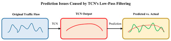
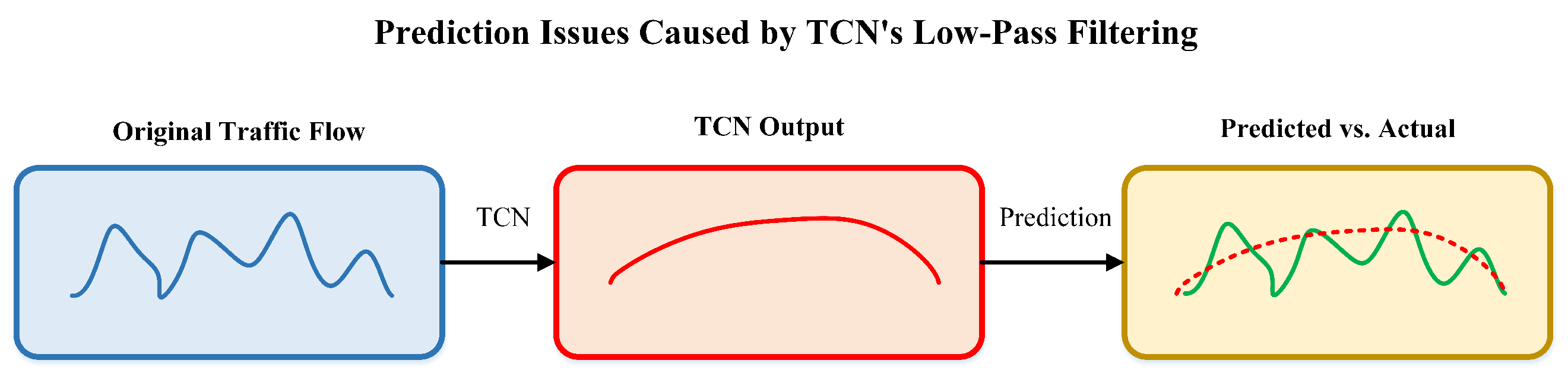
The temporal convolutional network (TCN) is a main component of the GWNET model. However, this paper identifies a long-overlooked inherent defect in TCN: its nature as a low-pass filter, which systematically attenuates high-frequency components in input signals. This characteristic may lead to loss of key event signals for traffic flow data rich in abrupt change information, as shown in Figure 4. Therefore, this section proposes a temporal feature enhancement strategy combining differential feature enhancement (DFA) and high-frequency residual compensation (HFRC) from the perspective of frequency-domain analysis.

Figure 4. Illustration of the Low-Pass Filtering Properties of TCN Module.

First, we analyze the low-pass filtering characteristic of TCN. Let the input signal be $X_n$, and the output of dilated causal convolution be as follows:

$$y_n=\sum _{k=0}^{K-1}{w}_k{x}_{n-d·k}$$

(27)

where K is the convolution kernel size, d is the dilation rate, and $w_k$ are learnable weights. Performing discrete-time Fourier transform (DTFT) [38] on Equation (27) yields its frequency response function:

$$H\left(\omega \right)=\sum _{k=0}^{K-1}{w}_k{e}^{-j\omega dk}$$

(28)

where $\omega \in [0,\pi ]$ is the normalized angular frequency. When convolution weights $w_k>0$, which is common in networks after ReLU activation, $\left|H\right(\omega \left)\right|$ significantly attenuates in high-frequency regions ($\omega \to \pi$) while maintaining high gain in low-frequency regions ($\omega \to 0$). This indicates that TCN inherently possesses low-pass filtering characteristics.

From a signal processing perspective, this characteristic stems from the weighted averaging nature of convolution operations over local windows. The cascading of multiple TCN layers further amplifies this effect.

4.4.1. Differential Feature Enhancement (DFA)

To address the above issue, this paper introduces a differential feature enhancement strategy at the input. Its core idea is to explicitly add high-pass filtered signals to the original input, providing the model with direct access to high-frequency information, thereby ensuring the preservation of high-frequency components before information enters TCN.

The first-order difference operator is defined as follows:

$$\Delta x_n=x_n-x_{n-1}$$

(29)

When performing frequency-domain analysis on Equation (29), its frequency response is

$$H_{\Delta }\left(\omega \right)=1-e^{-j\omega }=2j\sin (\omega /2)e^{-j\omega /2}$$

(30)

The corresponding magnitude response is

$$|H_{\Delta }\left(\omega \right)|=2|\sin (\omega /2)|$$

(31)

Analysis of Equation (31) shows that when $\omega =0$ (DC component) and $|H_{\Delta }|=0$, the signal is completely suppressed. When $\omega =\pi$ (highest frequency) and $|H_{\Delta }|=2$, the information gains maximum amplification. This indicates that the first-order difference operator is a high-pass filter, whose frequency response characteristics exactly complement the low-pass characteristics of TCN in the frequency domain.

Based on the above analysis, this paper defines the differential features as follows.

Definition 7 

(Differential Feature). Given the original input sequence $X\in {\mathbb{R}}^{B\times T\times N\times C}$, its first-order temporal difference is defined as

$$\Delta X_t=X_t-X_{t-1},t=2,3,\dots ,T.$$

(32)

For boundary conditions, set $\Delta X_1=0$ to maintain a consistent sequence length.

Definition 8 

(Enhanced Input). The differentially enhanced input is

$$\widehat{X}=[X\parallel \Delta X]\in {\mathbb{R}}^{B\times T\times N\times (C+1)},$$

(33)

where $\parallel$ denotes concatenation along the feature dimension. The original feature X preserves the absolute level information of the flow, while the differential feature $\Delta X$ explicitly encodes the rate of change between adjacent time steps.

From a frequency-domain perspective, the equivalent frequency response of enhanced input $\widehat{X}$ after TCN processing can be approximately expressed as

$$H_{eff}\left(\omega \right)\approx H_{TCN}\left(\omega \right)+H_{TCN}\left(\omega \right)·H_{\Delta }\left(\omega \right)$$

(34)

Since $H_{TCN}\left(\omega \right)$ has high gain in low-frequency regions and $H_{\Delta }\left(\omega \right)$ has high gain in high-frequency regions, their combination enables $H_{eff}\left(\omega \right)$ to maintain a relatively balanced response across the entire frequency band.

4.4.2. High-Frequency Residual Compensation (HFRC)

Although differential feature enhancement provides the model with access to high-frequency information at the input, these high-frequency components will still be attenuated layer by layer after processing through multiple TCN layers. Therefore, this paper further designs a high-frequency residual compensation mechanism at the output, utilizing the last observed value to adaptively correct prediction results.

Since the last observed value $X_T$ contains the latest and most accurate high-frequency information, and short-term predictions are highly correlated with $X_T$, while the smooth model output ${\widehat{Y}}_{model}$ tends to give smooth predictions lacking high-frequency details. Based on the above analysis, this paper decomposes the prediction target as follows:

$$Y=Y_{low}+Y_{high}$$

(35)

where $Y_{low}$ represents the low-frequency trend component, and $Y_{high}$ represents the high-frequency fluctuation component. Correspondingly, the main network output can be regarded as an approximation of the low-frequency component:

$${\widehat{Y}}_{model}\approx Y_{low}$$

(36)

The high-frequency component can be approximately compensated using the last observed value:

$$\alpha X_T+\beta \approx c·Y_{high}$$

(37)

where c is a certain proportionality coefficient. Combining Equations (36) and (37), the final prediction result can be expressed as

$${\widehat{Y}}_{final}={\widehat{Y}}_{model}+\alpha ·X_T+\beta$$

(38)

where ${\widehat{Y}}_{model}\in {\mathbb{R}}^{B\times T_f\times N\times 1}$ is the main network output, $X_T\in {\mathbb{R}}^{B\times N\times 1}$ represents the observation value at the last time step, $\alpha \in \mathbb{R}$ is the learnable compensation strength, and $\beta \in \mathbb{R}$ is the learnable bias term. For parameter initialization considerations, we set ${\alpha }_0=0.1$, making only a slight compensation initially to avoid disrupting the main network’s output; ${\beta }_0=0.0$ was also set, having no prior bias. During training, the model automatically adjusts these two parameters based on the loss function.

5. Experimental Setup

We evaluated the performance of CSHGCN on real-world highway traffic datasets. These data were collected from the California Department of Transportation Performance Measurement System (PeMS) [39] and are publicly accessible. Finally, we compare the results with several baseline methods to verify the accuracy and effectiveness of the proposed approach.

5.1. Datasets

To validate the effectiveness of the proposed method, we tested CSHGCN on four real-world traffic datasets: PEMS03, PEMS04, PEMS07, and PEMS08. They were collected by the California Performance Measurement System (PeMS) in real-time every 30 s. The raw traffic flow data were aggregated at 5 min intervals.

• PEMS03: This is a traffic flow dataset collected from Caltrans PeMS. It contains data from 358 sensors over a three-month period from 1 September 2018, to 30 November 2018. Traffic information is recorded at a rate of every 5 min, resulting in a total of 26,208 time slots.
• PEMS04: This is a traffic flow dataset collected from Caltrans PeMS. It contains data from 307 sensors over a two-month period from 1 January 2018, to 28 February 2018. Traffic information is aggregated every 5 min, totaling 16,992 time slices.
• PEMS07: This is a traffic flow dataset collected from Caltrans PeMS. It contains data from 883 sensors over a three-month period from 1 May 2017, to 6 August 2017. Traffic information is recorded at a rate of every 5 min, resulting in a total of 28,224 time steps.
• PEMS08: This is a traffic flow dataset collected from Caltrans PeMS. It contains data from 170 sensors in San Bernardino over a two-month period from 1 July 2016, to 31 August 2016. Traffic information is recorded at a rate of every 5 min, totaling 17,856 time slices.

5.2. Evaluation Metrics

In the experiments, the following three indicators are frequently used to evaluate the performance of the model.

$$\begin{array}{cc}\hfill \mathrm{MAE}(y,\widehat{y})& ={\displaystyle \frac{1}{T_f}}\sum _{i=1}^{T_f}|y_i-{\widehat{y}}_i|\hfill \end{array}$$

(39)

$$\begin{array}{cc}\hfill \mathrm{RMSE}(y,\widehat{y})& =\sqrt{{\displaystyle \frac{1}{T_f}}\sum _{i=1}^{T_f}{(y_i-{\widehat{y}}_i)}^2}\hfill \end{array}$$

(40)

$$\begin{array}{cc}\hfill \mathrm{MAPE}(y,\widehat{y})& ={\displaystyle \frac{1}{T_f}}\sum _{i=1}^{T_f}{\displaystyle \frac{|y_i-{\widehat{y}}_i|}{y_i}}\times 100\%\hfill \end{array}$$

(41)

where ${\widehat{y}}_i$ and $y_i$ represent the predicted and true values at time step i for all sensors, respectively, and $T_f$ is the prediction horizon.

5.3. Baseline Methods

We compare CSHGCN with the following baseline models:

• GWNET [18]: GWNET combines bidirectional diffusion convolution with dilated causal convolution and proposes an adaptive adjacency matrix to represent hidden spatial dependencies.
• STSGCN [40]: STSGCN proposes constructing local spatio-temporal graphs to extract spatio-temporal dependencies and designs multiple modules for different time periods to capture heterogeneity in local spatio-temporal graphs.
• MTGNN [19]: MTGNN designs a graph-learning module to capture unidirectional relationships between variables, mixed-hop propagation layers and dilated inception layers to extract spatio-temporal dependencies in time series, and combines graph convolution and temporal convolution modules to complete time series data prediction.
• STGODE [41]: STGODE adopts tensor-based ordinary differential equations (ODE) to extract spatio-temporal dynamics, designing semantic adjacency matrices and temporal dilated convolution structures; the former provides a more comprehensive understanding of the network, and the latter captures long-term temporal dependencies.
• STID [42]: STID learns spatio-temporal correlations in traffic data through spatial and temporal embeddings with MLP as the backbone.
• DDGCRN [43]: DDGCRN uses spatio-temporal embeddings and dynamic signals to extract dynamic spatio-temporal features, capturing spatio-temporal correlations in traffic data.
• BGCN [44]: BGCN treats the graph structure as a stochastic realization of a parameter generation model and approximates graph structure locality by performing Monte Carlo dropout on parameter graph structures.
• STWave [45]: STWave decomposes traffic data into stable trends and fluctuating events, then models trends and events through a dual-channel spatio-temporal network.
• STPGCN [46]: STPGCN designs a trainable embedding vector to characterize the spatio-temporal position of traffic nodes and integrates it into graph convolution to capture node-specific pattern features.
• PDG2Seq [47]: PDG2Seq designs a periodic feature selection module and a periodic dynamic graph convolutional gated recurrent unit to learn spatio-temporal dynamic features.

5.4. Experimental Configuration

We implemented CSHGCN using PyTorch 2.4.1 on Python 3.8. Experiments were conducted on a machine running Windows 10, equipped with a 13th Gen Intel(R) Core(TM) i9-13900K 3.00 GHz processor and an NVIDIA GeForce RTX 4090 GPU, with 24 GB memory. The parameter settings of our framework are the same as those of GWNET. All traffic datasets shared the following training setup.

Our objective was to predict traffic conditions for the next hour based on measurements from the past hour. We used the Adam optimizer (implemented in PyTorch [48], Meta AI, Menlo Park, CA, USA) to optimize all trainable variables for 100 epochs. The learning rate was initialized to 0.001. During training, each iteration randomly generated 64 pairs from the training dataset. All datasets were divided chronologically: 60% for training, 20% for validation, and 20% for testing. To ensure the statistical robustness of the results, all experiments were independently run under five different random seeds. The final reported performance metrics are the mean and standard deviation of these five runs, with both the mean and standard deviation rounded to two decimal places. In the experiments, Z-score normalization was applied to standardize the raw data:

$$X={\displaystyle \frac{X_r-\mathrm{mean}\left(X_r\right)}{\mathrm{std}\left(X_r\right)}}$$

(42)

Table 1 summarizes the key hyperparameters of the CSHGCN model used in all experiments. These settings remain consistent across all four benchmark datasets (PEMS03, PEMS04, PEMS07, PEMS08) to ensure fair comparison with baseline methods.

Table 1. Key hyperparameter configurations of the CSHGCN model.

Hyperparameter	Symbol	Value
Causal embedding dimension	d	10
Adaptive embedding dimension	c	10
Hidden layer dimension	H	32
Number of spatio-temporal layers	L	8
Dilated convolution base	K	2
Convolution kernel size	−	2
Hidden layer channels	−	32

6. Experimental Results and Analysis

6.1. Main Experimental Comparison

Table 2 shows the average MAE, RMSE, and MAPE results for 12 prediction horizons of CSHGCN and 10 representative baselines on four datasets. From this table, we can draw the following conclusions. Overall, CSHGCN performs excellently on the four benchmark datasets, achieving comprehensive optimal performance on PEMS07 and PEMS08, while being comparable or close to optimal models on PEMS03 and PEMS04.

Table 2. Performance comparison between CSHGCN and baseline models on four benchmark datasets. The best results are highlighted in bold.

Model	PEMS03			PEMS04			PEMS07			PEMS08
	MAE	RMSE	MAPE	MAE	RMSE	MAPE	MAE	RMSE	MAPE	MAE	RMSE	MAPE
GWNET	14.58	25.24	15.52%	18.99	30.28	13.91%	20.86	33.93	8.86%	14.83	23.64	9.47%
STSGCN	17.48	29.21	16.78%	21.19	33.65	13.90%	24.26	39.03	10.21%	17.16	26.80	10.96%
MTGNN	14.85	24.71	14.55%	19.17	31.17	13.38%	20.98	34.25	8.90%	15.16	24.10	10.14%
STGODE	15.76	27.30	15.84%	20.08	31.99	15.54%	21.68	36.39	9.52%	15.96	25.17	10.23%
STID	15.22	26.20	16.88%	18.39	29.89	12.80%	19.77	32.79	8.32%	14.22	23.46	9.30%
STWave	14.93	26.50	15.05%	20.01	30.39	12.89%	19.91	33.88	8.38%	13.82	23.53	9.35%
BGCN	14.35	25.28	14.47%	18.85	30.34	12.87%	20.05	32.86	8.45%	14.65	23.43	9.42%
DDGCRN	14.63	25.07	14.22%	18.45	30.51	12.19%	19.75	33.11	8.35%	14.45	23.75	9.40%
STPGCN	14.99	24.83	14.97%	18.52	30.53	12.63%	19.72	32.99	8.19%	13.92	23.85	9.25%
PDG2Seq	14.62	25.47	14.88%	18.24	30.08	12.09%	19.24	33.04	8.07%	13.84	23.37	9.27%
CSHGCN	14.53	24.42	14.57	18.26	29.72	12.61	19.12	31.92	8.02	13.58	22.53	9.08
(Ours)	±0.11	±0.15	±0.08%	±0.13	± 0.18	±0.07%	±0.10	±0.14	±0.06%	±0.09	±0.12	±0.05%

Note: The baseline model results are taken from the best reported values in their original papers or official implementations. The CSHGCN results are presented as mean ± standard deviation over five independent runs.

Overall Performance Analysis: CSHGCN achieves competitive prediction performance on all four datasets. Specifically, on the PEMS07 dataset, CSHGCN’s MAE, RMSE, and MAPE are 19.12, 31.92, and 8.02%, respectively, representing reductions of 0.83%, 3.39%, and 0.62% compared to PDG2Seq. On the PEMS08 dataset, MAE and MAPE are 13.58 and 9.08%, respectively, representing reductions of 8.43% and 4.12% compared to GWNET. On the PEMS03 and PEMS04 datasets, CSHGCN achieves optimal RMSE metrics, with MAE and MAPE comparable or close to the optimal baselines. Moreover, the small standard deviation of CSHGCN across five random runs indicates that its performance is stable and reproducible, and does not depend on specific random initializations.

Spatial Modeling Analysis: From the perspective of spatial dependency modeling, existing baseline methods exhibit obvious deficiencies. STSGCN relies on predefined static adjacency matrices and cannot capture dynamic spatial dependencies, resulting in significantly inferior performance on all datasets. Although GWNET and MTGNN introduce adaptive adjacency matrices, their symmetric design cannot model the directional propagation characteristics of traffic flow. CSHGCN, through the causal-enhanced adjacency matrix, decouples source and target node embeddings, enabling the learning of asymmetric upstream–downstream causal relationships.

Spatio-Temporal Joint Modeling Analysis: From the perspective of spatio-temporal feature fusion, recurrent network models such as DCRNN are limited by sequence dependencies and struggle to capture long-range temporal correlations. GWNET and MTGNN employ serial combinations of TCN and GCN, lacking an explicit modeling of joint transition probabilities of spatio-temporal states. The STMTM module introduced by CSHGCN is based on spatio-temporal Markov chain theory, explicitly learning conditional transition patterns in the form of $P\left(X_{n,m}\right|X_{n-1,m},X_{n,m-1})$ through temporal dependency encoders, spatial dependency encoders, and joint transition networks, enhancing the ability to capture complex spatio-temporal dynamics.

Temporal Modeling Analysis: TCN-based models such as GWNET and MTGNN have inherent low-pass filtering characteristics in temporal feature extraction, leading to sluggish responses to high-frequency abrupt change signals in traffic flow. CSHGCN provides explicit high-frequency change information to the model through differential feature enhancement and corrects the smoothing effect of TCN through a high-frequency residual compensation mechanism at the output stage. This design gives CSHGCN stronger tracking abilities during periods of intense flow fluctuations.

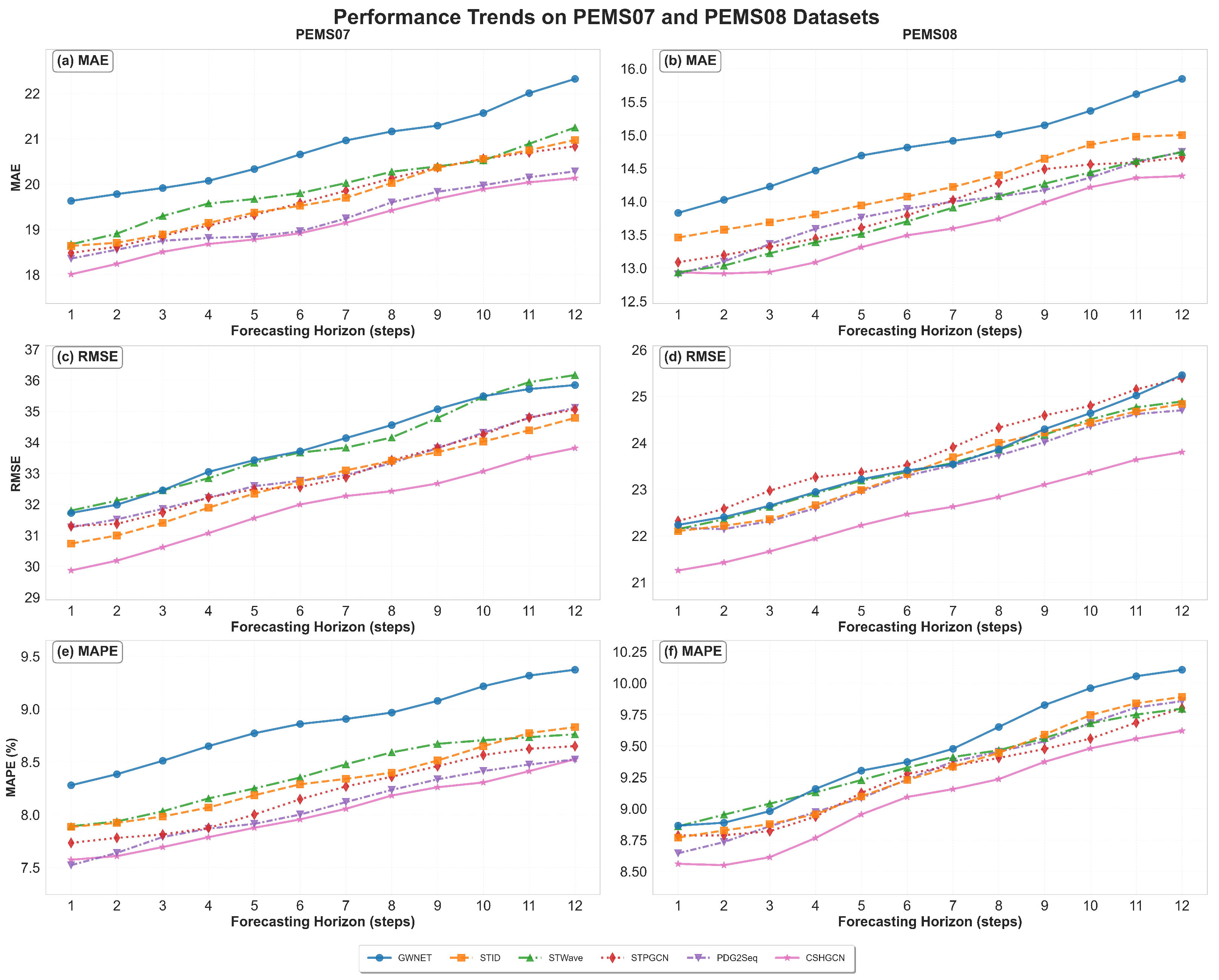
Performance Across Different Prediction Horizons: Figure 5 shows the performance of CSHGCN at each horizon on four datasets. For clear visualization, we only display six methods: GWNET, STID, STWave, STPGCN, PDG2Seq, and CSHGCN. From this figure, we find that as the prediction interval increases, the prediction performance of all three methods significantly declines, indicating that long-term traffic prediction faces greater challenges than short-term traffic prediction. Notably, CSHGCN consistently exhibits superior performance at all time steps on the PEMS07 and PEMS08 datasets.

Figure 5. Performance comparison of models across different prediction horizons.

6.2. Ablation Study

To deeply investigate the contribution of each core module in CSHGCN, we design the following variants for ablation experiments on the PeMS08 dataset:

• w/o Causal: Remove the causal-enhanced adjacency matrix, retaining only the standard adaptive adjacency matrix.
• w/o STMTM: Remove the spatio-temporal Markov transition module, reverting to the standard TCN+GCN serial structure.
• w/o HF: Remove the high-frequency-aware enhancement mechanism, including differential feature enhancement (DFA) and high-frequency residual compensation (HFRC).
• w/o CS: Simultaneously remove the causal adjacency matrix and STMTM module.
• w/o CH: Simultaneously remove the causal adjacency matrix and high-frequency-aware mechanism.
• w/o SH: Simultaneously remove the STMTM module and high-frequency-aware mechanism.
• CSHGCN: The complete model containing all innovative modules.

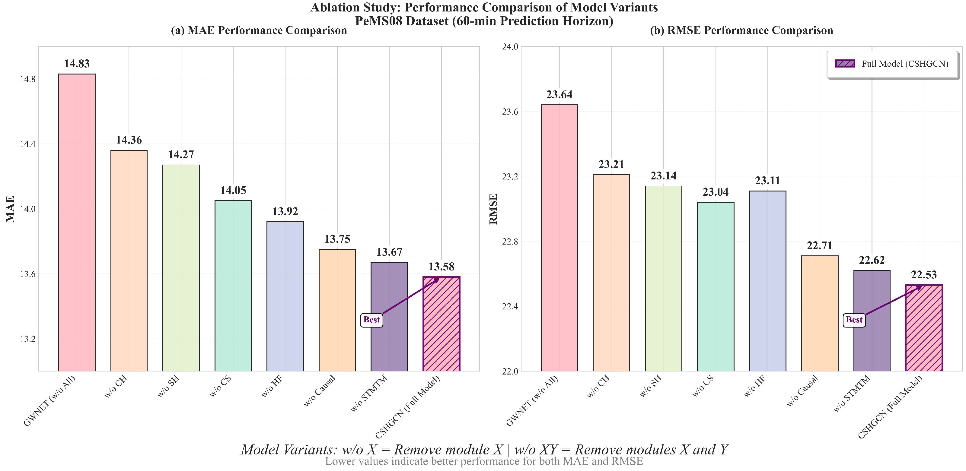
w/o Causal: Removing the causal adjacency matrix increases MAE to 13.75, a performance degradation of 1.25%. This validates that the symmetric adaptive matrix in GWNET lacks explicit causal directionality, whereas our explicit decoupling of source/target embeddings ensures asymmetry, offering clear advantages in directional scenarios.

w/o STMTM: Removing the STMTM module increases MAE to 13.67 (0.66% degradation). Although its individual contribution appears modest, STMTM provides crucial theoretical framework innovation, explicitly modeling joint transition probabilities where GWNET only implicitly combines temporal and spatial features.

w/o HF: Removing the high-frequency enhancement mechanism causes the largest performance drop among single-module removals, increasing MAE by 2.50% to 13.92. This significant impact confirms that TCN’s inherent low-pass filtering severely smooths crucial high-frequency traffic signals. Our DFA and HFRC mechanisms provide effective frequency-domain complementarity and compensation with minimal parameter overhead (only 1 differential channel and 2 scalars), demonstrating exceptional parameter efficiency.

From Table 3, significant module synergy effects can be observed. For instance, the performance drop for w/o CH (5.75%) is substantially greater than the simple sum of the drops from w/o HF (2.50%) and w/o Causal (1.25%). The extra 2.00% degradation stems from the loss of synergy between the modules. Similarly, the drop for w/o CS (3.46%) exceeds the sum of individual removals. This super-additive effect indicates that the modules are not independent: the high-frequency mechanism preserves full frequency-domain information, the causal matrix builds accurate spatial propagation paths upon it, and STMTM further learns joint spatio-temporal transitions. As visualized in Figure 6, the absence of any module diminishes the effectiveness of the others. Together, they synergistically achieve an overall performance improvement relative to the GWNET baseline.

Table 3. Ablation study results on the PeMS08 dataset (Horizon = 12), where all results are the average of five independent runs.

Model Variant	MAE	RMSE	MAPE	Performance Drop vs. Full
w/o CH	14.36	23.21	9.31%	+5.75%
w/o SH	14.27	23.14	9.28%	+5.09%
w/o CS	14.05	23.04	9.22%	+3.46%
w/o HF	13.92	23.11	9.17%	+2.50%
w/o Causal	13.75	22.71	9.13%	+1.25%
w/o STMTM	13.67	22.62	9.11%	+0.66%
CSHGCN (Full)	13.58	22.53	9.08%	-

Note: Performance drop = (average MAE of the variant model − average MAE of the full model)/average MAE of the full model × 100%.

Figure 6. Performance comparison of model variants.

6.3. Efficiency Analysis

This section systematically compares CSHGCN with mainstream baseline models from three dimensions: parameter count, single-epoch training time, and single-epoch evaluation time. The results are summarized in Table 4. All experiments are conducted on a server equipped with an NVIDIA RTX 4090 GPU (24GB memory), using the PeMS08 dataset.

Table 4. Efficiency comparison of different models (PeMS08 dataset).

Model	Parameters (M)	Training Time (s/epoch)	Evaluation Time (s/epoch)
GWNET	0.305471	33.278	8.140
STSGCN	1.144420	26.747	1.613
MTGNN	0.433340	13.553	1.075
BGCN	0.285040	22.552	5.705
STPGCN	0.196116	38.990	0.890
PDG2Seq	1.151957	24.020	1.960
CSHGCN	0.267640	25.558	5.970

(1) Parameter Scale Analysis

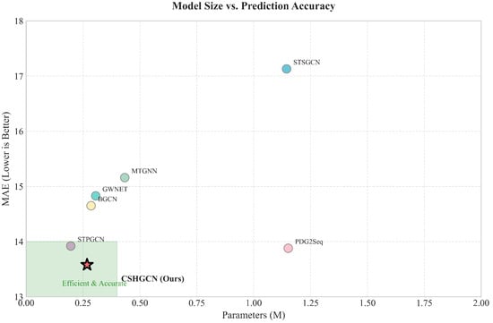
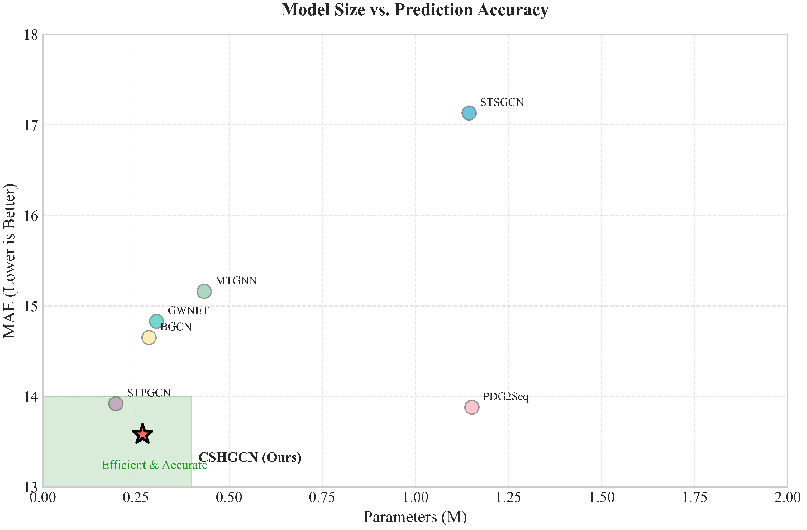
Figure 7 illustrates the trade-off between parameter count and prediction error (MAE). Models range from lightweight (e.g., STPGCN at 0.19M parameters) to heavy (e.g., STSGCN and PDG2Seq exceeding 1.15M). CSHGCN, with a moderate 0.27M parameters, achieves excellent MAE, indicating high prediction accuracy. Although slightly larger than STPGCN, CSHGCN offers significantly better accuracy, reflecting effective model design. Notably, CSHGCN’s parameter count is only 23.4% of STSGCN’s, yet it delivers comparable or superior performance, demonstrating high parameter efficiency. This efficiency stems from: (a) the factorized embedding strategy (source/target), reducing spatial complexity from $O\left(N^2\right)$ to $O\left(2Nd\right)$; (b) the explicit modeling in STMTM avoiding redundant computations; and (c) the lightweight HFRC mechanism adding negligible overhead.

Figure 7. Comparison of model parameters vs. prediction error on PEMS08 dataset.

(2) Training and Evaluation Efficiency

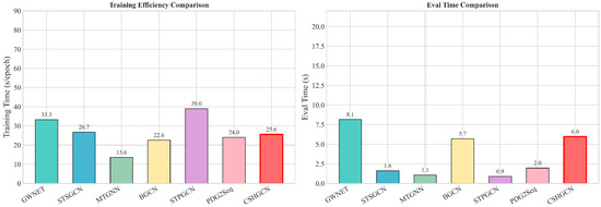
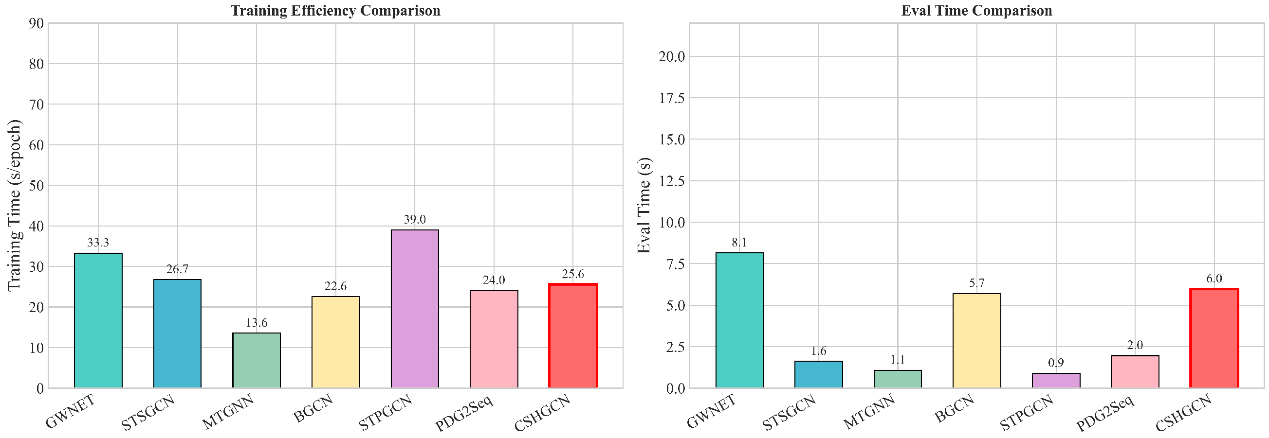
As shown in Figure 8, MTGNN (13.55 s/epoch) and BGCN (22.55 s/epoch) are the fastest to train. CSHGCN’s training time (25.56 s/epoch) is slightly faster than GWNET’s and reasonable compared to other models. The differences stem from architectural designs: MTGNN uses efficient mixed-hop propagation, while STSGCN’s local graph design reduces global computation. CSHGCN’s overhead relative to GWNET is minimal, primarily due to the STMTM forward pass and the virtually cost-free HFRC. Its evaluation time (5.97 s/epoch) supports feasible real-time deployment. Overall, the training and evaluation time of CSHGCN is within an acceptable range considering the improvement in accuracy. It should be noted that the actual deployment latency may also be affected by system integration and data preprocessing overheads.

Figure 8. Comparison of model running time on PEMS08 dataset.

6.4. Visualization Analysis

To intuitively showcase CSHGCN’s predictive capabilities and its advantages over baselines, we provide a systematic visualization from three perspectives: traffic flow prediction curves, prediction error analysis, and spatio-temporal heatmaps.

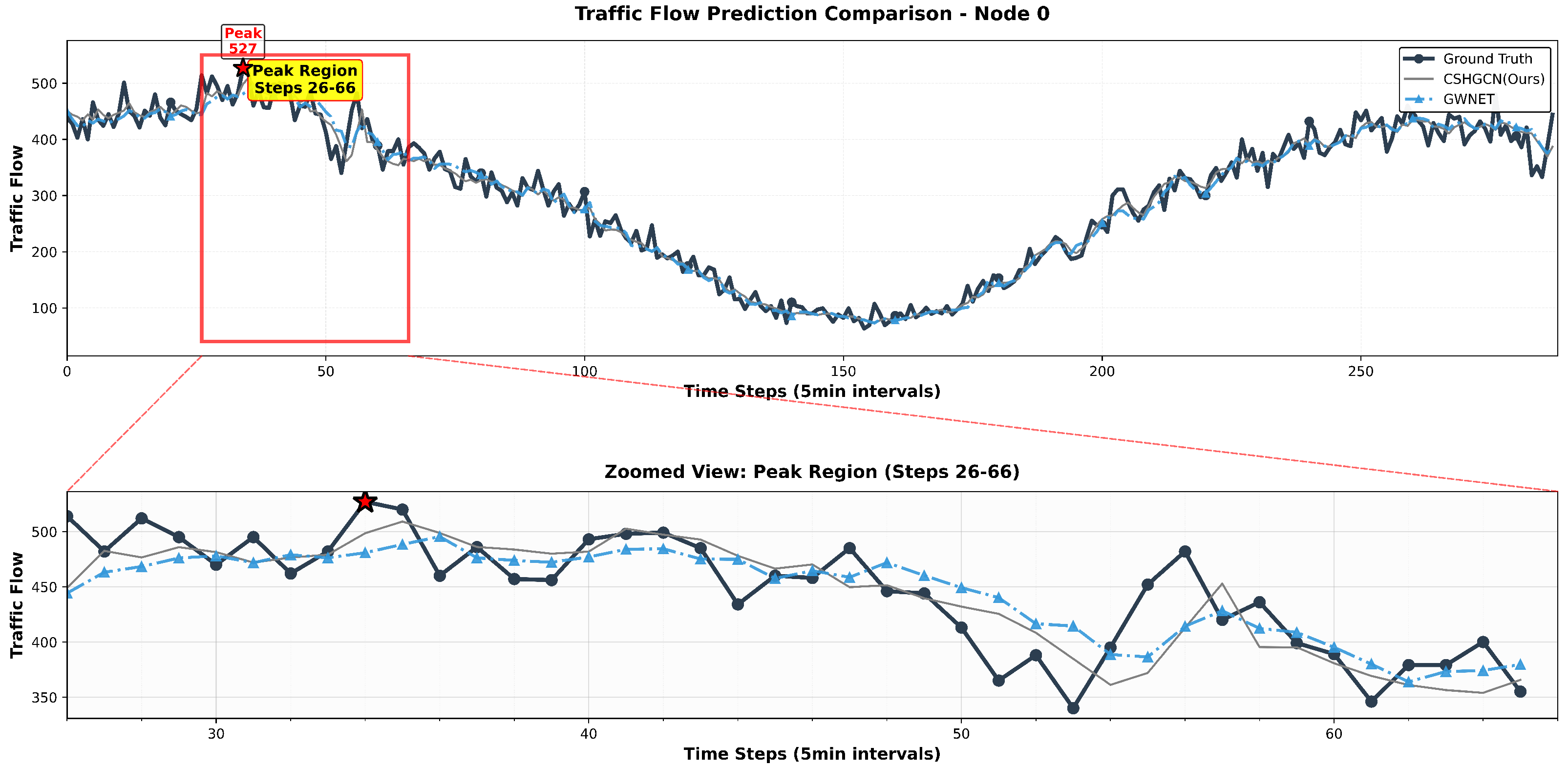
Figure 9 shows a comparison of CSHGCN and GWNET predictions over a full day (288 five-minute steps). CSHGCN’s predictions adhere more closely to the ground truth, especially during abrupt change periods like the morning rush (steps 26–66, see inset). This demonstrates CSHGCN’s superior ability to capture turning points and peaks, attributable to the STMTM module’s state transition awareness and the HFRC mechanism’s preservation of high-frequency details.

Figure 9. Comparison of traffic flow prediction curves for different models over a one-day period.

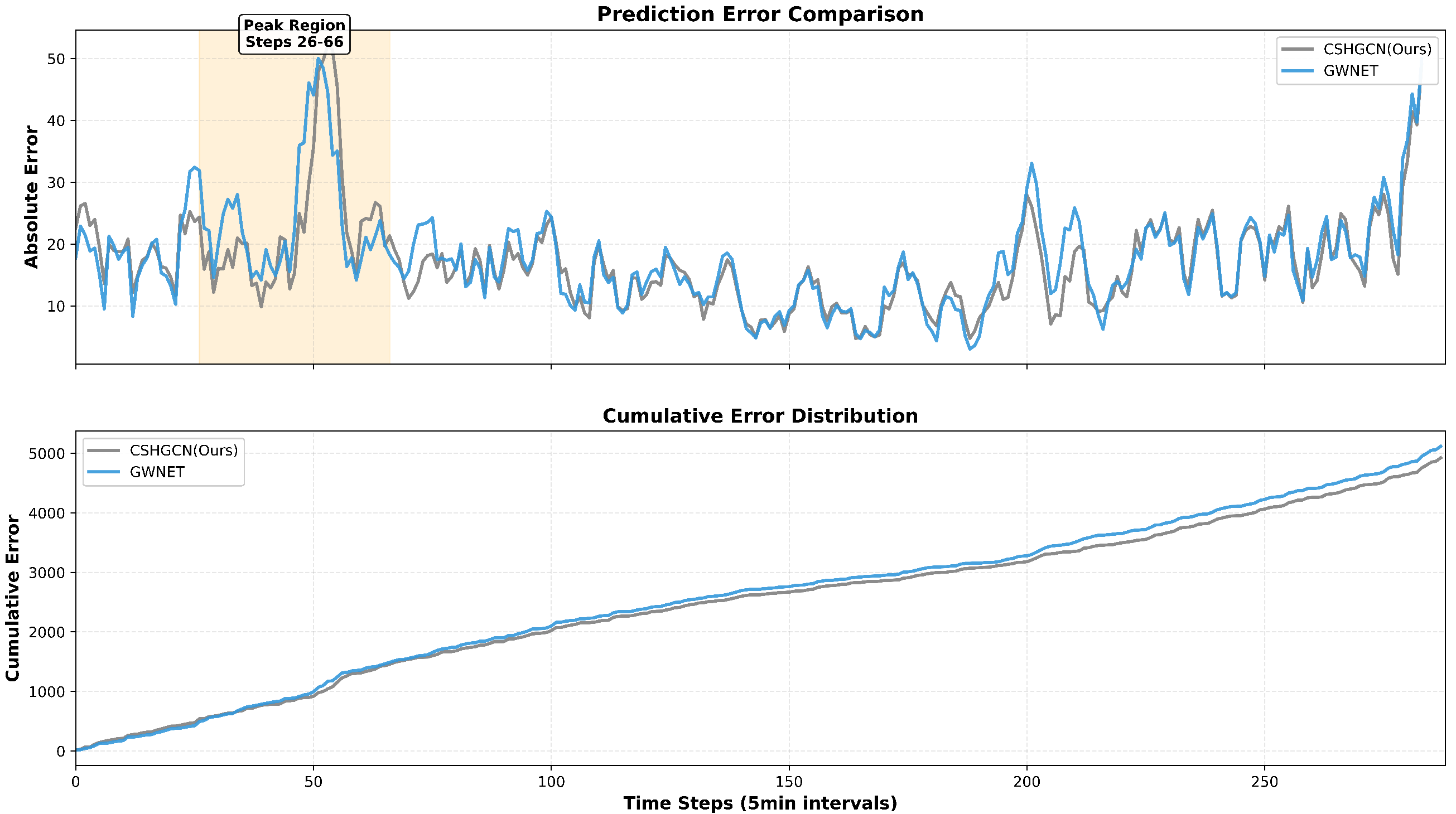
Figure 10 quantifies model performance differences from two perspectives. The top plot shows instantaneous prediction error per time step, where CSHGCN’s error is lower than GWNET’s for most steps. The bottom plot shows cumulative error over time (steps 20–66). CSHGCN’s cumulative error curve remains consistently below GWNET’s, and the gap widens over time. By the end of 288 steps, GWNET’s cumulative error is 5000, while CSHGCN’s is only 4000—a reduction of approximately 20%. This highlights CSHGCN’s stability and its ability to avoid error accumulation in long-term forecasting.

Figure 10. Comparison of prediction errors.

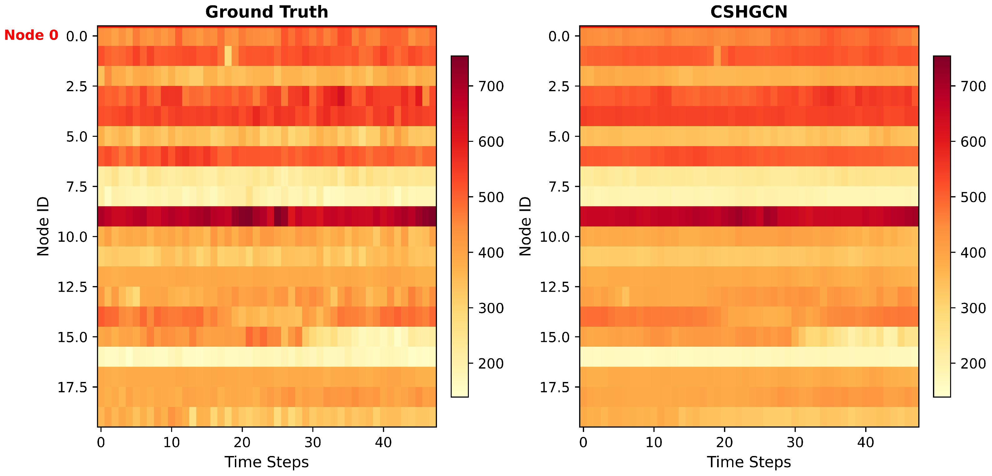
Figure 11 presents an overall comparison of multi-node prediction effects from a spatial dimension. Depicts traffic flow for 20 representative nodes over 4 h. The CSHGCN prediction heatmap aligns remarkably well with the ground truth, successfully reconstructing the spatio-temporal evolution structure. It accurately captures the position and intensity of traffic peaks (dark red regions), confirming its effectiveness in modeling complex spatial dynamics.

Figure 11. Heatmap of traffic flow for selected nodes.

7. Discussion

(1) Design Advantages of Causal-Enhanced Adjacency Matrix: Traditional GNN-based traffic prediction models commonly employ symmetric adjacency matrices, which implicitly assume bidirectional, equal-strength influences between nodes. However, traffic flow propagation inherently exhibits clear directionality: congestion spreads from upstream to downstream, and tidal flow during peak hours exhibits unidirectional dominance. This physical reality fundamentally contradicts the symmetry assumption. This paper breaks through this limitation by decoupling source and target node embeddings, enabling the model to naturally learn asymmetric causal influence relationships. Ablation studies show that removing the causal adjacency matrix leads to decreased prediction accuracy. This result verifies the judgment that symmetric matrices struggle to accurately capture the directional propagation characteristics of traffic flow. Notably, the parameter increment of the causal adjacency matrix is only $O\left(Nd\right)$, compared to the $O\left(N^2\right)$ complexity of directly learning a complete asymmetric matrix, achieving a good balance between parameter efficiency and modeling capability.

(2) Theoretical Value of the Spatio-Temporal Markov Transition Module: Most existing spatio-temporal prediction models adopt serial or parallel architectures of graph convolution and temporal convolution, treating spatio-temporal feature extraction as two independent processes. The fundamental problem with this design is the lack of explicit characterization of the joint evolution patterns of traffic states across spatio-temporal dimensions. This paper introduces the theoretical framework of spatio-temporal Markov chains (STMC), integrating the rigorous probabilistic framework of STMC into deep spatio-temporal prediction models through the collaborative work of temporal dependency encoders, spatial dependency encoders, and joint transition networks. Furthermore, the adaptive gating mechanism in the module enables the data-driven adjustment of update intensity, which is crucial for coping with non-stationary traffic flow. Experiments demonstrate that STMTM exhibits significant advantages in traffic flow prediction, with improvements in MAE.

(3) Design Motivation for High-Frequency Residual Compensation: Temporal convolutional networks, as mainstream temporal modeling tools in traffic prediction, have an inherent low-pass filtering characteristic that is often overlooked. This paper designs a dual enhancement strategy from the perspective of frequency-domain complementarity. Differential feature enhancement utilizes the high-pass characteristics of first-order differences to provide the model with direct access to high-frequency information at the input; high-frequency residual compensation then uses the last observed value to correct prediction results at the output, restoring high-frequency details smoothed by TCN. Ablation studies show that removing the high-frequency enhancement mechanism leads to the most significant performance degradation among the three single-module removals. It is worth emphasizing that this mechanism introduces only one differential channel and two scalar parameters, demonstrating the simplicity and high parameter efficiency of the design. This approach has strong generality and can be extended to other TCN-based spatio-temporal prediction models.

(4) Synergistic Relationships Between Modules: The three design modules in this study enhance traffic flow prediction from three dimensions: spatial causality, spatio-temporal joint evolution, and temporal frequency-domain feature preservation, forming complementary synergistic relationships. The causal adjacency matrix ensures correct directionality in spatial information propagation, STMTM guarantees theoretical completeness in spatio-temporal coupled evolution modeling, and high-frequency compensation compensates for inherent defects in temporal convolution. Ablation studies show that removing any one module leads to performance degradation, and the complete model’s effect is superior to any combination of two modules, verifying the synergistic gains of the three innovations across different modeling dimensions.

8. Conclusions

This study proposes a causal-enhanced spatio-temporal Markov graph convolutional network (CSHGCN) to address key challenges in non-stationary traffic flow prediction. First, a causally enhanced asymmetric adjacency matrix is constructed by decoupling source and target node embeddings. This design explicitly models directional causal dependencies, overcoming the limitation of symmetric graph convolutions in capturing upstream–downstream propagation. Second, a spatio-temporal Markov transition module (STMTM) is introduced based on spatio-temporal Markov chain theory. By integrating temporal and spatial dependency encoders with a joint transition network, the STMTM incorporates a rigorous probabilistic framework to explicitly learn conditional state transitions across spatio-temporal dimensions. Furthermore, from a frequency-domain perspective, we identify the inherent low-pass filtering characteristic of temporal convolutional networks (TCNs) and propose a dual strategy of differential feature enhancement and high-frequency residual compensation. This strategy effectively counteracts the tendency of TCNs to smooth out critical high-frequency fluctuations, with minimal additional parameters. Comprehensive experiments on four public benchmark datasets demonstrate that CSHGCN outperforms ten state-of-the-art baseline methods in terms of MAE, RMSE, and MAPE. In summary, this work presents a novel modeling paradigm for spatio-temporal forecasting involving directional and non-stationary dynamics. Future research will focus on exploring more complex dynamic causal structures and improving model generalization across diverse scenarios.

References

- Walch, M.; Schirrer, A.; Neubauer, M. Impact assessment of cooperative intelligent transport systems (C-ITS): A structured literature review. Eur. Transp. Res. Rev. 2025, 17, 11. [Google Scholar] [CrossRef] [Scilit]
- Ganin, A.A.; Mersky, A.C.; Jin, A.S.; Kitsak, M.; Linkov, I. Resilience in intelligent transportation systems (ITS). Transp. Res. Part C Emerg. Technol. 2019, 100, 318–329. [Google Scholar] [CrossRef] [Scilit]
- Liu, Z.; Wang, C. Design of Traffic Emergency Response System Based on Internet of Things and Data Mining in Emergencies. IEEE Access 2019, 7, 113950–113962. [Google Scholar] [CrossRef] [Scilit]
- Emek, S.; Ildrar, G.; Gurbuzer, Y. Application of Long Short-Term Memory and XGBoost Model for Carbon Emission Reduction: Sustainable Travel Route Planning. Sustainability 2025, 17, 10802. [Google Scholar] [CrossRef] [Scilit]
- Shahriari, S.; Ghasri, M.; Sisson, S.A.; Waller, S.T. Ensemble of ARIMA: Combining parametric and bootstrapping technique for traffic flow prediction. Transp. A Transp. Sci. 2020, 16, 1552–1573. [Google Scholar] [CrossRef] [Scilit]
- Kipf, T.N.; Welling, M. Semi-Supervised Classification with Graph Convolutional Networks. arXiv 2016, arXiv:1609.02907. [Google Scholar]
- Bai, S.; Kolter, J.Z.; Koltun, V. An Empirical Evaluation of Generic Convolutional and Recurrent Networks for Sequence Modeling. arXiv 2018, arXiv:1803.01271. [Google Scholar] [CrossRef] [Scilit]
- Carrizosa, E.; Olivares-Nadal, A.V.; Ramirez-Cobo, P. A sparsity-controlled vector autoregressive model. Biostatistics 2017, 18, 244–259. [Google Scholar] [CrossRef] [Scilit] [PubMed]
- Hyndman, R.J.; Athanasopoulos, G. Forecasting: Principles and Practice, 3rd ed.; OTexts: Melbourne, Australia, 2021. [Google Scholar]
- Dixon, K.W.; Lanzante, J.R.; Nath, M.J.; Hayhoe, K.; Stoner, A.; Radhakrishnan, A.; Balaji, V. Evaluating the stationarity assumption in statistically downscaled climate projections: Is past performance an indicator of future results? Clim. Change 2016, 135, 395–408. [Google Scholar] [CrossRef] [Scilit]
- Li, J.; Mei, X.; Prokhorov, D.; Tao, D. Deep Neural Network for Structural Prediction and Lane Detection in Traffic Scene. IEEE Trans. Neural Netw. Learn. Syst. 2017, 28, 690–703. [Google Scholar] [CrossRef] [Scilit]
- Zhao, J.; Deng, F.; Cai, Y.; Chen, J. Long short-term memory - Fully connected (LSTM-FC) neural network for PM(2.5) concentration prediction. Chemosphere 2019, 220, 486–492. [Google Scholar] [CrossRef] [Scilit]
- Zhang, J.; Zheng, Y.; Qi, D. Deep Spatio-Temporal Residual Networks for Citywide Crowd Flows Prediction. arXiv 2016, arXiv:1610.00081. [Google Scholar]
- Lee, K.; Rhee, W. DDP-GCN: Multi-graph convolutional network for spatiotemporal traffic forecasting. Transp. Res. Part C Emerg. Technol. 2022, 134, 103466. [Google Scholar] [CrossRef] [Scilit]
- Yu, B.; Yin, H.; Zhu, Z. Spatio-temporal Graph Convolutional Neural Network: A Deep Learning Framework for Traffic Forecasting. arXiv 2017, arXiv:1709.04875. [Google Scholar]
- Li, Y.; Yu, R.; Shahabi, C.; Liu, Y. Graph Convolutional Recurrent Neural Network: Data-Driven Traffic Forecasting. arXiv 2017, arXiv:1707.01926. [Google Scholar]
- Hamilton, W.L.; Ying, R.; Leskovec, J. Inductive Representation Learning on Large Graphs. In Proceedings of the 31st International Conference on Neural Information Processing Systems (NeurIPS), Long Beach, CA, USA, 4–9 December 2017; Curran Associates Inc.: Red Hook, NY, USA, 2017; pp. 1024–1034. [Google Scholar]
- Wu, Z.; Pan, S.; Long, G.; Jiang, J.; Zhang, C. Graph WaveNet for Deep Spatial-Temporal Graph Modeling. In Proceedings of the 28th International Joint Conference on Artificial Intelligence, Macao, China, 10–16 August 2019; AAAI Press: Palo Alto, CA, USA, 2019; pp. 1907–1913. [Google Scholar]
- Wu, Z.; Pan, S.; Long, G.; Jiang, J.; Chang, X.; Zhang, C. Connecting the Dots: Multivariate Time Series Forecasting with Graph Neural Networks. In Proceedings of the 26th ACM SIGKDD International Conference on Knowledge Discovery & Data Mining, Virtual Event, CA, USA, 23–27 August 2020; ACM: New York, NY, USA, 2020; pp. 753–763. [Google Scholar]
- Bai, L.; Yao, L.; Li, C.; Wang, X.; Wang, C. Adaptive Graph Convolutional Recurrent Network for Traffic Forecasting. arXiv 2020, arXiv:2007.02842. [Google Scholar] [CrossRef] [Scilit]
- Vaswani, A.; Shazeer, N.; Parmar, N.; Uszkoreit, J.; Jones, L.; Gomez, A.N.; Kaiser, L.; Polosukhin, I. Attention Is All You Need. In Proceedings of the 31st International Conference on Neural Information Processing Systems (NeurIPS), Long Beach, CA, USA, 4–9 December 2017; Curran Associates Inc.: Red Hook, NY, USA, 2017; pp. 5998–6008. [Google Scholar]
- Wei, X.; Xia, D.; Li, Y.; Liu, Z. Attention-based spatial-temporal synchronous graph convolution networks for traffic flow forecasting. Appl. Intell. 2025, 55, 557–570. [Google Scholar] [CrossRef] [Scilit]
- Zheng, C.; Fan, X.; Wang, C.; Qi, J. GMAN: A Graph Multi-Attention Network for Traffic Prediction. arXiv 2019, arXiv:1911.08415. [Google Scholar]
- Zhou, H.; Zhang, S.; Peng, J.; Zhang, S.; Li, J.; Xiong, H.; Zhang, W. Informer: Beyond Efficient Transformer for Long Sequence Time-Series Forecasting. arXiv 2020, arXiv:2012.07436. [Google Scholar]
- Wu, H.; Xu, J.; Wang, J.; Long, M. Autoformer: Decomposition Transformers with Auto-Correlation for Long-Term Series Forecasting. In Advances in Neural Information Processing Systems, Virtual, 6–14 December 2021; Curran Associates, Inc.: Red Hook, NY, USA, 2021; pp. 22419–22430. [Google Scholar]
- Zhou, T.; Ma, Z.; Wen, Q.; Wang, X.; Sun, L.; Jin, R. FEDformer: Frequency Enhanced Decomposed Transformer for Long-term Series Forecasting. In Proceedings of the 39th International Conference on Machine Learning, Baltimore, MA, USA, 17–23 July 2022; PMLR: Brookline, MA, USA, 2022; pp. 27268–27286. [Google Scholar]
- Veličković, P.; Cucurull, G.; Casanova, A.; Romero, A.; Liò, P.; Bengio, Y. Graph Attention Networks. In Proceedings of the 6th International Conference on Learning Representations (ICLR), Vancouver, BC, Canada, 30 April–3 May 2018. [Google Scholar]
- Choi, J.; Choi, H.; Hwang, J.; Park, N. Graph Neural Controlled Differential Equations for Traffic Forecasting. In Proceedings of the AAAI Conference on Artificial Intelligence, Virtual, 2–9 February 2021; AAAI Press: Palo Alto, CA, USA, 2021; pp. 6367–6374. [Google Scholar]
- Zhang, X.; Huang, C.; Xu, Y.; Xia, L.; Dai, P.; Bo, L.; Zhang, Y.; Qiao, H. Traffic Flow Forecasting with Spatial-Temporal Graph Diffusion Network. In Proceedings of the AAAI Conference on Artificial Intelligence, Virtual, 2–9 February 2021; AAAI Press: Palo Alto, CA, USA, 2021; pp. 15008–15015. [Google Scholar]
- Lan, S.; Ma, Y.; Huang, W.; Wang, W.; Yang, H.; Li, P. DSTAGNN: Dynamic Spatial-Temporal Aware Graph Neural Network for Traffic Flow Forecasting. In Proceedings of the 39th International Conference on Machine Learning, Baltimore, MA, USA, 17–23 July 2022; PMLR: Brookline, MA, USA, 2022; pp. 11906–11917. [Google Scholar]
- Peng, H.; Du, B.; Liu, M.; Liu, M.; Ji, S.; Wang, S.; Zhang, Y.; He, L. Dynamic graph convolutional network for long-term traffic flow prediction with reinforcement learning. Inf. Sci. 2021, 578, 401–416. [Google Scholar] [CrossRef] [Scilit]
- Schölkopf, B. Causality for Machine Learning. In Probabilistic and Causal Inference: The Works of Judea Pearl; Association for Computing Machinery: New York, NY, USA, 2022; pp. 765–804. [Google Scholar]
- Kipf, T.; Fetaya, E.; Wang, K.-C.; Welling, M.; Zemel, R. Neural Relational Inference for Interacting Systems. In Proceedings of the 35th International Conference on Machine Learning (ICML), Stockholm, Sweden, 10–15 July 2018; PMLR: Brookline, MA, USA, 2018; pp. 2688–2697. [Google Scholar]
- Huang, J.; Meng, Y.; Liu, F.; Liu, C.; Li, H. Modeling and predicting inventory variation for multistage steel production processes based on a new spatio-temporal Markov model. Comput. Ind. Eng. 2022, 164, 107854. [Google Scholar] [CrossRef] [Scilit]
- Hammer, H.L.; Yazidi, A. Parameter estimation in abruptly changing dynamic environments using stochastic learning weak estimator. Appl. Intell. 2018, 48, 4096–4112. [Google Scholar] [CrossRef] [Scilit]
- Cai, R.; Huang, X.; Chen, W.; Li, Z.; Hao, Z. Temporal latent variable structural causal model for causal discovery under external interferences. Neurocomputing 2025, 640, 130281. [Google Scholar] [CrossRef] [Scilit]
- Kumralbas, Z.; Tumer, B. Incremental learning of spatio-temporal Markov chains: An introductory theoretical framework for composite domain Markov chains. Inf. Sci. 2025, 721, 120–135. [Google Scholar] [CrossRef] [Scilit]
- Song, H.; Fan, L.; Liu, J.; Sun, H.; Chen, Y. Efficient Frequency Estimation of Sinusoid Based on Autocorrelation and Discrete Time Fourier Transform. Circ. Syst. Signal Process. 2024, 43, 4675–4689. [Google Scholar] [CrossRef] [Scilit]
- Chen, C.; Petty, K.F.; Skabardonis, A.; Varaiya, P.; Jia, Z. Freeway Performance Measurement System: Mining Loop Detector Data. Transp. Res. Rec. 2001, 1748, 96–102. [Google Scholar] [CrossRef] [Scilit]
- Song, C.; Lin, Y.; Guo, S.; Wan, H. Spatial-Temporal Synchronous Graph Convolutional Networks: A New Framework for Spatial-Temporal Network Data Forecasting. In Proceedings of the AAAI Conference on Artificial Intelligence, New York, NY, USA, 7–12 February 2020; AAAI Press: Palo Alto, CA, USA, 2020; pp. 914–921. [Google Scholar]
- Fang, Z.; Long, Q.; Song, G.; Xie, K. Spatial-Temporal Graph ODE Networks for Traffic Flow Forecasting. In Proceedings of the 27th ACM SIGKDD Conference on Knowledge Discovery and Data Mining, Virtual, 14–18 August 2021; ACM: New York, NY, USA, 2021; pp. 364–373. [Google Scholar]
- Shao, Z.; Zhang, Z.; Wang, F.; Wei, W.; Xu, Y. Spatial-Temporal Identity: A Simple yet Effective Baseline for Multivariate Time Series Forecasting. In Proceedings of the 31st ACM International Conference on Information & Knowledge Management, Atlanta, GA, USA, 17–21 October 2022; ACM: New York, NY, USA, 2022; pp. 4454–4458. [Google Scholar]
- Weng, W.; Fan, J.; Wu, H.; Hu, Y.; Tian, H.; Zhu, F.; Wu, J. A Decomposition Dynamic graph convolutional recurrent network for traffic forecasting. Pattern Recognit. 2023, 142, 109670. [Google Scholar] [CrossRef] [Scilit]
- Fu, J.; Zhou, W.; Chen, Z. Bayesian graph convolutional network for traffic prediction. Neurocomputing 2024, 582, 127507. [Google Scholar] [CrossRef] [Scilit]
- Fang, Y.; Qin, Y.; Luo, H.; Zhao, L.; Wang, J. STWave+: A Multi-Scale Efficient Spectral Graph Attention Network with Long-Term Trends for Disentangled Traffic Flow Forecasting. IEEE Trans. Knowl. Data Eng. 2024, 36, 2671–2685. [Google Scholar] [CrossRef] [Scilit]
- Zhao, Y.; Lin, Y.; Wen, H.; Sun, F.; Chen, T. Spatial-Temporal Position-Aware Graph Convolution Networks for Traffic Flow Forecasting. IEEE Trans. Intell. Transp. Syst. 2023, 24, 8650–8666. [Google Scholar] [CrossRef] [Scilit]
- Fan, J.; Weng, W.; Chen, Q.; Zhang, Y.; Chen, J. PDG2Seq: Periodic Dynamic Graph to Sequence Model for Traffic Flow Prediction. Neural Netw. 2025, 183, 106941. [Google Scholar] [CrossRef] [Scilit] [PubMed]
- Kingma, D.P.; Ba, J. Adam: A Method for Stochastic Optimization. arXiv 2014, arXiv:1412.6980. [Google Scholar]
Disclaimer/Publisher’s Note: The statements, opinions and data contained in all publications are solely those of the individual author(s) and contributor(s) and not of MDPI and/or the editor(s). MDPI and/or the editor(s) disclaim responsibility for any injury to people or property resulting from any ideas, methods, instructions or products referred to in the content. |
© 2026 by the authors. Licensee MDPI, Basel, Switzerland. This article is an open access article distributed under the terms and conditions of the Creative Commons Attribution (CC BY) license.