Stabilization of Nonlinear Coupled Parametric Oscillators of Mathieu’s Type in Fractal Space

Abstract

In this work, the Renormalization Method (RM) is used to analyze the dynamics of a nonlinear two-degree-of-freedom (2DOF) system under parametric excitation, with a focus on fractal vibration behavior. This procedure comprises transforming the system into a comparable form. An equivalent linearized model is produced by isolating the system’s nonlinear interactions using a two-scale formulation and mean-square analysis. The non-autonomous fractal equations are transformed into an autonomous representation using the RM, and then the system is described in traditional derivative form using El-Dib’s fractal transformation. The fractal-coupled Mathieu system’s stability behavior can be effectively identified using this framework. An agreement with the analytical solutions is shown by numerical results. All things considered, the integrated RM-based approach provides a reliable tool for forecasting and managing intricate nonlinear fractal systems.

1. Introduction

Because nonlinear models exhibit a wide range of behaviors and linearization techniques have inherent limitations, methods for analyzing nonlinear dynamical systems continue to be an active research area. Numerical integration frequently falls short of providing broad understanding of global dynamics, stability boundaries, and parametric trends, even though it can yield precise solutions for particular parameter sets. This restriction is especially noticeable in multi-degree-of-freedom (MDOF) systems with substantial coupling effects and strong nonlinearities [1,2,3]. Beyond case-specific numerical results, non-perturbative analytical techniques are essential in illuminating the underlying dynamic mechanisms in this context.

Recent years have witnessed a surge in research focusing on vibration control and nonlinear dynamic analysis across diverse engineering scenarios, with both experimental characterization and analytical methodology achieving notable progress. On the application front, scholars have carried out in-depth exploration on the vibration performance optimization of materials and structures: Wang et al. [4] proposed a hybrid method combining image processing and vibro-acoustic characterization to optimize the acoustic vibration performance of Sitka spruce by analyzing grain inhomogeneity; An et al. [5] assessed the blade vibration induced by two-phase unsteady leakage flow in subsea counter-rotating axial flow compressors, providing a theoretical basis for the stability design of marine rotating machinery; Han et al. [6] investigated the vibration excitation mechanism of dual-idler gear-rack transmission systems with defects and completed corresponding optimization; and Zhang et al. [7] conducted coupling vibration analysis for inspection robots landing on high-voltage transmission lines, addressing the dynamic stability problem of special operation equipment. In the field of adhesive joint structures, Londhe & Jagtap [8] revealed the vibrational behavior of MWCNT-reinforced single and cross-overlap adhesive joints through experiments and finite element analysis. For the analytical solution of nonlinear vibration models, Song et al. [9] applied He’s frequency formula to the nonlinear free vibration of conical beams and discussed its educational implications. In addition to structural vibration, the homotopy perturbation method has also been widely used in solving nonlinear systems: Alshomrani et al. [10] and He and El-Dib [11]adopted this method to solve nonlinear epidemic models; Hendy et al. [12] explored the fractional order thermo-viscoelasticity problem of polymer micro-rods with and without energy dissipation; and Moussa et al. [13] successfully solved the Duffing–Van der Pol equation using the homotopy perturbation method, enriching the analytical toolkit for strongly nonlinear systems. However, most of the above studies are based on traditional integer-order derivative models, and there is still a lack of systematic research on the dynamic characteristics of multi-degree-of-freedom parametric oscillators in fractal space, which is the core issue to be addressed in this paper.

A useful framework for examining intricate nonlinear dynamics under periodic excitation, particularly in stability evaluation, is fractal geometry. Phase portraits, basin boundaries, and Poincaré maps all exhibit fractal patterns, which are highly sensitive to initial conditions and system parameters and frequently indicate the beginning of instability or chaos. While fractal attractors define stability limits, Moon and Holmes [14] showed that fractal basin boundaries are closely related to instability in nonlinear vibratory systems. Thompson and Stewart [15] reported similar findings, linking fractal basin boundaries to chaotic responses in nonlinear oscillators. As a result, fractal-based modelling [16,17,18] offers a potent diagnostic tool for capturing scale-invariant behaviors seen in actual engineering structures and for differentiating between stable and unstable responses in periodically excited systems.

The analytical treatment of nonlinear oscillations has been further extended by recent developments in fractal calculus. Leibniz and chain rules, Picard-type theorems, and other fundamental results for fractal derivatives were established by Santiesteban et al. [19] and compared with classical and conformable formulations. For fractal systems like the Toda lattice and Duffing oscillators, analytical approximations based on homotopy perturbation techniques have also been successfully applied, producing results that closely match numerical simulations, especially in the vicinity of classical limits [20].

El-Dib’s fractal transformation, which converts fractal derivatives into equivalent classical derivatives and permits the use of conventional analytical methods without ignoring the effects of fractality, is a major contribution to this field. By using this method to derive modified Mathieu–Duffing-type equations, El-Dib and colleagues were able to obtain precise analytical solutions under both non-resonant and subharmonic resonance conditions [21,22,23]. This transformation is particularly appropriate for engineering applications since it offers a useful link between fractal modeling and classical vibration theory.

A key component of nonlinear dynamics is parametric excitation, which is defined by periodic changing of system parameters like stiffness or damping [24,25]. When excitation frequencies interact with the natural frequencies of the system, it can cause parametric resonance, bifurcations, and complex oscillatory responses [26,27,28]. The relationship between parametric forcing and intrinsic nonlinearities is captured by the nonlinear Mathieu equation, which is enhanced by cubic stiffness factors. This leads to varied dynamic phenomena, including resonance tongues, stability boundaries, and chaotic regimes [29,30,31,32,33,34,35,36]. These phenomena are essential to consider in engineering applications, such as fluid systems, electrical circuits, and mechanical constructions, where resonance control and stability are vital for performance and safety [37].

By extending this framework, coupled nonlinear differential equations with parametric excitation and Duffing-type stiffness effects are incorporated into the nonlinear two-degree-of-freedom (2DOF) Mathieu oscillator [38,39,40,41]. Internal resonance, modal energy transfer, and stability transitions brought on by nonlinear coupling can all be described by this model. It has been extensively used to simulate vibrations in electromechanical and MEMS devices where nonlinear coupling cannot be avoided, as well as in beams, bridges, and aerospace structures, including flutter phenomena [42,43,44,45]. Internal and parametric resonances have a significant impact on the stability of these systems, resulting in chaotic dynamics, amplitude modulation, and mode interaction [46,47]. Vibration control, structural integrity, and energy harvesting applications in civil, mechanical, and aerospace engineering all depend on an understanding of these principles [48].

Techniques beyond standard perturbation methods are needed to tackle the analytical difficulties presented by such systems. Strong tools for evaluating strongly nonlinear oscillators without depending on tiny parameters are provided by frequency formulation techniques created by Chun-Hui He, Ji-Huan Heet al. [49]. Renormalization-based techniques, on the other hand, provide non-perturbative solutions for parametric nonlinear oscillators without the secular divergence that comes with traditional series expansions. These techniques provide correct amplitude–frequency relationships even at high excitation levels and facilitate effective stability and bifurcation analysis by converting non-autonomous systems into equivalent autonomous forms [50].

El-Dib’s frequency methodology is a particularly useful analytical tool for parametric and coupled nonlinear oscillators among these methods. It is especially appropriate for Helmholtz–Duffing–Mathieu-type systems since it concurrently accounts for nonlinear stiffness, damping, parametric excitation, and coupling effects. Under non-perturbative conditions, the technique yields precise estimates of effective natural frequencies that capture the complete dynamic behavior of systems that are susceptible to instability and resonance [51].

Inspired by these advances, the current work uses sophisticated analytical methods to examine the dynamics and stability of a 2DOF fractal nonlinear Mathieu oscillator with damping. A mean-square method efficiently linearizes the nonlinear system, allowing parametric excitation, nonlinear coupling, and modal interactions to be analyzed in a single framework. The suggested approach shows good agreement with numerical simulations and provides analytical answers for the system’s linear autonomous form. In addition to offering useful advice for engineering applications like vibrating structures and MEMS, where exact control of nonlinear dynamic behavior is crucial, the results offer fresh perspectives on the stabilizing function of fractal parameters [52,53].

The remainder of the paper is organized in this manner. Section 2 highlights the problem’s theoretical and practical motives while discussing its significance and scientific relevance. The linearization process for the two-degree-of-freedom (2DOF) fractal system is presented in Section 3. Specifically, the self-conversion of the governing equations into an autonomous system is introduced in Section 3.1, the transformation of the fractional derivative into its conventional counterpart is described in Section 3.2, and the dependence of the resulting fractal system on the physical parameters is established in Section 3.3. A methodical plan for transforming the coupled Equations (38) and (39) into an analogous set of decoupled equations is developed in Section 4. Section 5 offers numerical validation of the suggested methodology, with Section Identification and Detection of Stability Predictions concentrating on the detection and identification of stability predictions. Lastly, Section 6 summarizes the study’s key findings and conclusions, and suggests possible future research.

2. Importance and Scientific Relevance of the Problem

A damped fractal 2DOF nonlinear parametric system describes the interaction between two coupled oscillators, incorporating time-dependent excitation, linear coupling, damping, and nonlinear stiffness. Understanding the dynamic behavior necessitates analyzing the individual and combined effects of these parameters, revealing stability boundaries, resonance, mode-interaction, and susceptibility to external forces. These findings are crucial in engineering and applied physics for designing and controlling vibrating structures and advanced systems, significantly enhancing system performance.

The following is an expression for the damped fractal nonlinear 2DOF parametric system:

$${\displaystyle \frac{dx}{d{t}^{2\alpha }}}+{\mu }_1{\displaystyle \frac{dx}{d{t}^{\alpha }}}+\left(a_1+q_1\cos \left(2{\omega }_0{t}^{\alpha }\right)\right)x+\left(a_3+q_3\cos \left(2{\omega }_0{t}^{\alpha }\right)\right)y+{\gamma }_1{x}^3+{\eta }_1{x}^{2}y=0,$$

(1)

$${\displaystyle \frac{dy}{d{t}^{2\alpha }}}+{\mu }_2{\displaystyle \frac{dy}{d{t}^{\alpha }}}+\left(a_2+q_2\cos \left(2{\omega }_0{t}^{\alpha }\right)\right)y+\left(a_4+q_4\cos \left(2{\omega }_0{t}^{\alpha }\right)\right)x+{\gamma }_2{y}^3+{\eta }_2{y}^2\hspace{0.17em}x=0.$$

(2)

where x($t^{\alpha }$) and y($t^{\alpha }$) denote the displacement responses of the two coupled subsystems, and the fractional order α satisfies $0<\alpha <1$. The parameter ${\omega }_0$represents the excitation frequency, ${\mu }_i$denotes the damping coefficients, and $a_i$ are the constant natural frequencies of the nonparametric oscillators. The term $q_{ij}$ correspond to the amplitudes of the parametric modulation of the natural frequencies, ${\eta }_i$ denotes the nonlinear coupling coefficients, and ${\gamma }_i$represents the Duffing-type nonlinear stiffness coefficients. This model shows how beams or plates move in response to recurring external loads. Both parametric stimulation and material nonlinearities cause nonlinear vibrations in the system.

The initial conditions are regularly assumed as follows:

$$x(0)=A,\hspace{0.17em}{\displaystyle \frac{dx(0)}{d{t}^{\alpha }}}=0\hspace{0.17em}\hspace{0.17em}\mathrm{and}\hspace{0.17em}\hspace{0.17em}y(0)=B,\hspace{0.17em}{\displaystyle \frac{dy(0)}{d{t}^{\alpha }}}=0.\hspace{0.17em}$$

(3)

Equations (1) and (2) describe a system that comprises two connected nonlinear Mathieu–Duffing oscillators influenced by damping effects within a fractal dynamical framework. These equations capture the behavior of two coupled oscillators whose motion occurs in a fractal space, an environment where the shape of the medium or the path of motion exhibits self-similar, scale-dependent properties.

In this work, the fractal dimension and associated parameters are employed to depict scale-dependent and memory effects that standard integer-order models do not capture. Physically, the fractal dimension quantifies the degree of temporal complexity and irregular energy distribution in the system response, whereas the fractal parameters govern the severity of these non-classical effects. From an engineering standpoint, changing the fractal dimension influences effective stiffness, damping, and energy dissipation, all of which have a direct impact on resonance and stability properties. The observed increase in stability with decreasing fractal dimension supports the physical relevance of these factors. The manuscript has been updated to clarify this interpretation.

In this context, a two-scale fractal derivative, which considers the influence of fractal geometry on the system’s temporal evolution, replaces the conventional time derivative. The multi-scale nature of energy transmission, damping, and nonlinear interactions in fractal media can be represented in the model through this adjustment. Consequently, the inherent scaling rules embedded in the fractal background govern the linked oscillatory motion, as well as the parametric excitation and the linear and nonlinear restoring forces.

The definition of the two-scale fractal derivative is as follows:

$$D_t^{(\alpha )}f(t)=\underset{\Delta t\to 0}{\lim }{\displaystyle \frac{f(t+\Delta t^{\alpha })-f(t)}{\Delta t^{\alpha }}}.$$

(4)

The two-scale transform converts fractal derivatives into smooth-space counterparts, replacing rescaled derivatives with traditional integer-order derivatives. This mapping allows the application of standard analytical techniques while maintaining the influence of fractal geometry. It reinterprets fractal oscillator equations using conventional oscillatory dynamics, bridging the gap between classical mechanics and the scale-dependent nature of fractal space, thereby facilitating analysis of complex behavior through traditional frameworks.

The substitution τ = t^α, a common approach within the two-scale framework of fractal space, can be employed to convert the fractal systems described in Equations (1)–(3) into a more manageable form. This transformation simplifies the governing equations while preserving the core influence of fractal geometry by re-expressing the original fractal-time dynamics in terms of a rescaled smooth variable, τ.

$$x^{″}+{\mu }_1{x}^{\prime }+\left(a_1+q_1\cos \left(2{\omega }_0\tau \right)\right)x+\left(a_3+q_3\cos \left(2{\omega }_0\tau \right)\right)y+{\gamma }_1{x}^3+{\eta }_1{x}^{2}y=0,$$

(5)

$$y^{″}+{\mu }_2{y}^{\prime }+\left(a_2+q_2\cos \left(2{\omega }_0\tau \right)\right)y+\left(a_4+q_4\cos \left(2{\omega }_0\tau \right)\right)x+{\gamma }_2{y}^3+{\eta }_2{y}^2\hspace{0.17em}x=0,$$

(6)

and

$$x(0)=A,\hspace{0.17em}{x}^{\prime }(0)=0\hspace{0.17em}\hspace{0.17em}\mathrm{and}\hspace{0.17em}\hspace{0.17em}y(0)=B,\hspace{0.17em}{y}^{\prime }(0)=0.\hspace{0.17em}$$

(7)

The dash above signifies differentiation with respect to the rescaled variable τ. The two-scale fractal calculus framework, which employs a carefully chosen rescaled variable to transform fractal derivatives into conventional derivatives systematically, directly transforms the fractal system in Equations (1) and (2) into the smooth-space forms shown in Equations (5) and (6).

3. Linearization Procedure for the 2DOF Fractal System

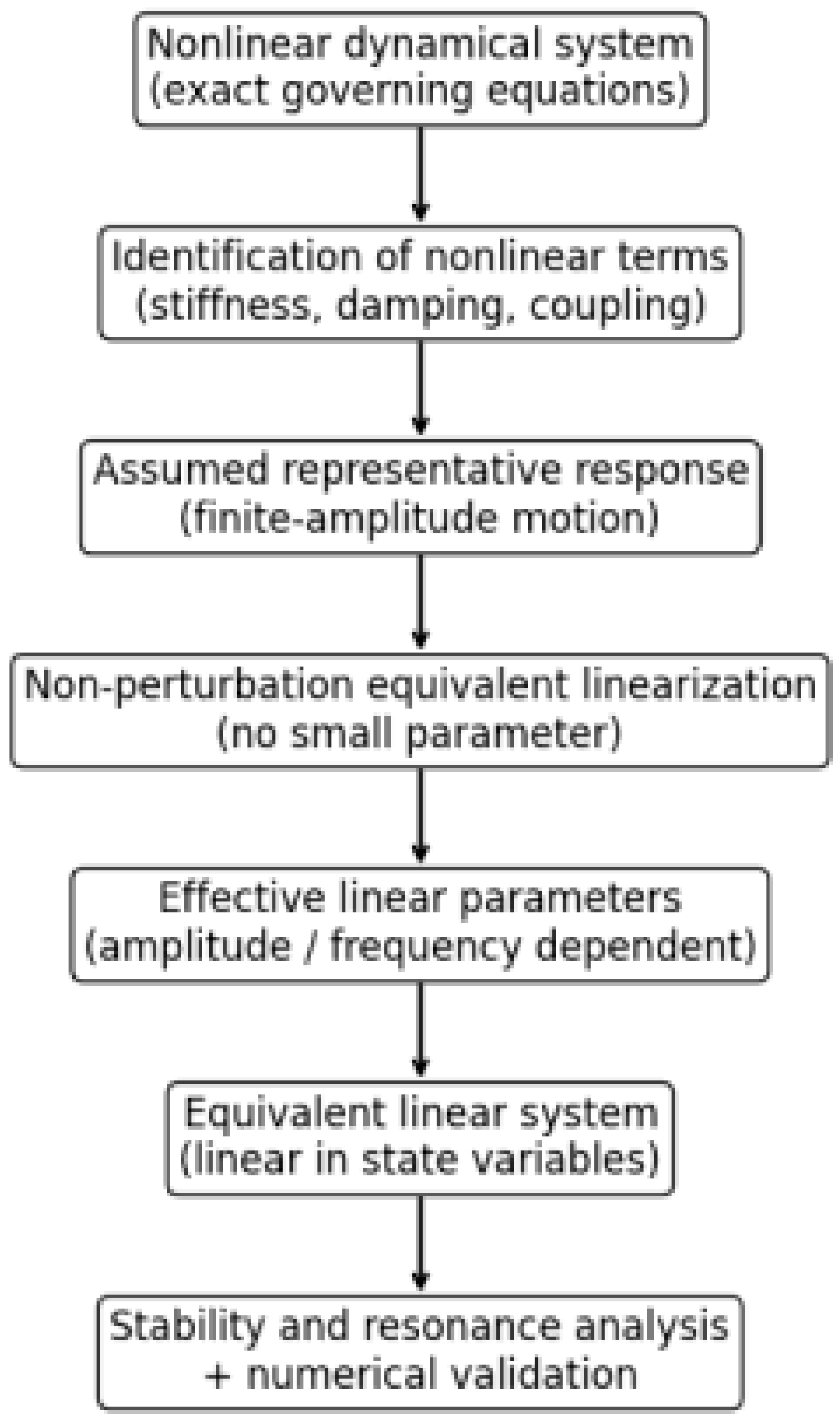
When adopting a non-perturbation approach, a nonlinear system is converted to a linearized form without assuming a small parameter or using a perturbation series. This procedure maintains the fundamental dynamic characteristics of the original system over a specific response range. It starts by formulating the nonlinear equations of motion in their precise form, incorporating all nonlinear factors without scaling. An assumed response, reflective of the system’s expected behavior, is then selected. Nonlinear terms are substituted with linear equivalents based on a consistency condition that minimizes discrepancies over one motion period. This process yields amplitude-dependent linear stiffness and damping coefficients while keeping the system linear in state variables, permitting the application of standard linear analysis techniques as shown in the flowchart below in Figure 1. The model’s accuracy is validated against direct numerical integration of the nonlinear system, confirming that it effectively captures stability and resonance within the operational range. This methodology serves as a robust framework for analyzing strongly nonlinear systems when traditional perturbation methods do not succeed.

By replacing the nonlinear effects in the governing equations with carefully chosen linear approximations, an equivalent linearized model of the system is obtained that retains the key dynamical features while enabling the use of traditional linear analysis methods. This linearization relies on the Mean Square Approach [42], a well-regarded method for providing accurate approximations of nonlinear systems and facilitating their analysis. It is particularly effective for examining response characteristics, stability, and resonance. The fractal 2DOF nonlinear system in Equations (5) and (6) can be converted into their corresponding linear form by assuming trial solutions with different frequencies for each degree of freedom.

$$x_0(\tau )=A\cos {\Omega }_1\tau \mathrm{and} y_0(\tau )=B\cos {\Omega }_2\tau .$$

(8)

The oscillation amplitudes are represented by A and B in this formulation, and the total frequencies Ω₁ and Ω₂ are determined later in the process. It is possible to estimate the mean square features and directly substitute them into the controlling nonlinear variables by assuming harmonic motion through this trial solution. This method simplifies the nonlinear model to a linearized 2DOF system.

The corresponding mean square displacement values can be obtained using the trial solutions specified in Equation (8). These formulations provide a useful analytical tool for examining the dynamic behavior of the system and simplifying coupled nonlinear interactions.

$${\overline{x}}^2={\displaystyle \frac{1}{2T_1}}{\displaystyle \underset{0}{\overset{T_1}{\int }}{x}_0^{2}d\tau }={\displaystyle \frac{1}{4}}{A}^2\hspace{0.17em}\hspace{0.17em}\hspace{0.17em}\mathrm{and}\hspace{0.17em}\hspace{0.17em}\hspace{0.17em}\hspace{0.17em}{\overline{y}}^2={\displaystyle \frac{1}{2T_2}}{\displaystyle \underset{0}{\overset{T_2}{\int }}{y}_0^{2}d\tau }={\displaystyle \frac{1}{4}}{B}^2.$$

(9)

This procedure produces mean-square formulations that provide a systematic approach to handling the intricate characteristics of nonlinear systems. They facilitate the extraction of important dynamic parameters and provide a linearized representation of potentially complex nonlinear interactions. This approach is widely recognized for studying nonlinear vibration phenomena because it provides reasonably accurate results while simplifying evaluation. Therefore, we recall the nonlinear variables in Equations (5) and (6), as follows:

$$x^{″}+{\mu }_1{x}^{\prime }+\left(a_1+q_1\cos \left(2{\omega }_0\tau \right)\right)x+\left(a_3+q_3\cos \left(2{\omega }_0\tau \right)\right)y+f_1(x)x+f_3(x)y=0,$$

(10)

$$y^{″}+{\mu }_2{y}^{\prime }+\left(a_2+q_2\cos \left(2{\omega }_0\tau \right)\right)y+\left(a_4+q_4\cos \left(2{\omega }_0\tau \right)\right)x+f_2(y)y+f_4(y)x=0,$$

(11)

where the definitions of the nonlinear stiffening functions are

$$\begin{array}{l}{f}_1(x)={\gamma }_1{x}^2,\hspace{0.17em}\hspace{0.17em}{f}_3(x)={\eta }_1{x}^2,\hspace{0.17em}\hspace{0.17em}\\ f_2(y)={\gamma }_2{y}^2,\hspace{0.17em}\hspace{0.17em}{f}_4(y)={\eta }_2{y}^2.\end{array}$$

(12)

Previous studies of nonlinear two-degree-of-freedom parametric systems have examined nonlinearities up to the fifth order (x⁵) [54,55,56], unlike many classical models that focus on cubic terms (x³) [57,58]. Cubic models capture weakly nonlinear behavior near primary resonance, accurately describing small to moderate oscillation amplitudes and yielding symmetric hardening or softening characteristics. In contrast, the quintic term becomes significant at larger amplitudes, modifying amplitude–frequency relationships and resonance curve shapes, which can enhance or suppress nonlinear saturation. This results in changes to stability regions, bifurcation thresholds, and energy exchange. In fractal nonlinear parametric systems, the x⁵ term significantly impacts stability by interacting with fractal parameters, causing higher-order nonlinear effects to persist over broader amplitudes and affecting conditions where cubic models assume stability.

Examining the nonlinear stiffness expressions in (10) and (11) reveals that both have a dominating odd component and an extra, secondary odd stiffness contribution. Because the odd functions control the system’s frequency, the dominated frequencies are established as

$$\begin{array}{l}{\varpi }_1^2=\underset{\begin{array}{l}x\to \overline{x},y\to \overline{y}\\ \hspace{0.17em}\hspace{0.17em}\hspace{0.17em}\hspace{0.17em}\hspace{0.17em}\hspace{0.17em}\hspace{0.17em}n\to 3\end{array}}{\lim }n{f}_1(x)={\displaystyle \frac{3}{4}}{A}^2{\gamma }_1,\\ {\varpi }_2^2=\underset{\begin{array}{l}x\to \overline{x},y\to \overline{y}\\ \hspace{0.17em}\hspace{0.17em}\hspace{0.17em}\hspace{0.17em}\hspace{0.17em}\hspace{0.17em}\hspace{0.17em}n\to 3\end{array}}{\lim }n{f}_2(y)={\displaystyle \frac{3}{4}}{B}^2{\gamma }_2.\end{array}$$

(13)

Further, the secondary frequencies are derived as

$$\begin{array}{l}{\varpi }_3^2=\underset{\begin{array}{l}x\to \overline{x},y\to \overline{y}\\ \hspace{0.17em}\hspace{0.17em}\hspace{0.17em}\hspace{0.17em}\hspace{0.17em}\hspace{0.17em}\hspace{0.17em}n\to 3\end{array}}{\lim }n{f}_3(x)={\displaystyle \frac{3}{4}}{A}^2{\eta }_1,\\ {\varpi }_4^2=\underset{\begin{array}{l}x\to \overline{x},y\to \overline{y}\\ \hspace{0.17em}\hspace{0.17em}\hspace{0.17em}\hspace{0.17em}\hspace{0.17em}\hspace{0.17em}\hspace{0.17em}n\to 3\end{array}}{\lim }n{f}_4(y)={\displaystyle \frac{3}{4}}{B}^2{\eta }_2,\end{array}$$

(14)

where n is the power of the nonlinearity. As demonstrated by Equations (10) and (11), the method is particularly useful for linearizing the coupled nonlinearities, and is applied to problems involving nonlinear vibrations [59,60,61]. Therefore, the modified natural frequencies are obtained by incorporating the influence of the frequency-dependent stiffness characteristics into Equations (10) and (11). A more accurate representation of the dynamic behavior, especially under different stiffness conditions, can be obtained by incorporating these updated frequencies into the system equations. Accurately analyzing the system’s stability and resonant responses in the presence of parametric stimulation and nonlinear interactions requires this refinement.

Consequently, the following is an expression for the damped linear coupled Mathieu’s equations that result from the linearization of the nonlinear system:

$$x^{″}+{\mu }_1{x}^{\prime }+\left(a_1+{\varpi }_1^2+q_1\cos \left(2{\omega }_0\tau \right)\right)x+\left(a_3+{\varpi }_3^2+q_3\cos \left(2{\omega }_0\tau \right)\right)y=0,$$

(15)

$$y^{″}+{\mu }_2{y}^{\prime }+\left(a_2+{\varpi }_2^2+q_2\cos \left(2{\omega }_0\tau \right)\right)y+\left(a_4+{\varpi }_4^2+q_4\cos \left(2{\omega }_0\tau \right)\right)x=0.$$

(16)

As shown in Equations (15) and (16), this linearization streamlines the analysis by substituting strong linear approximations for nonlinear interactions. This makes it easy to use modal analysis, stability evaluation, and other traditional methods. The method provides a solid basis for understanding the central dynamics of the system by precisely accounting for coupling effects and parametric excitation. By comparing the responses of the linearized and original nonlinear systems, the linearization’s faithfulness is verified numerically.

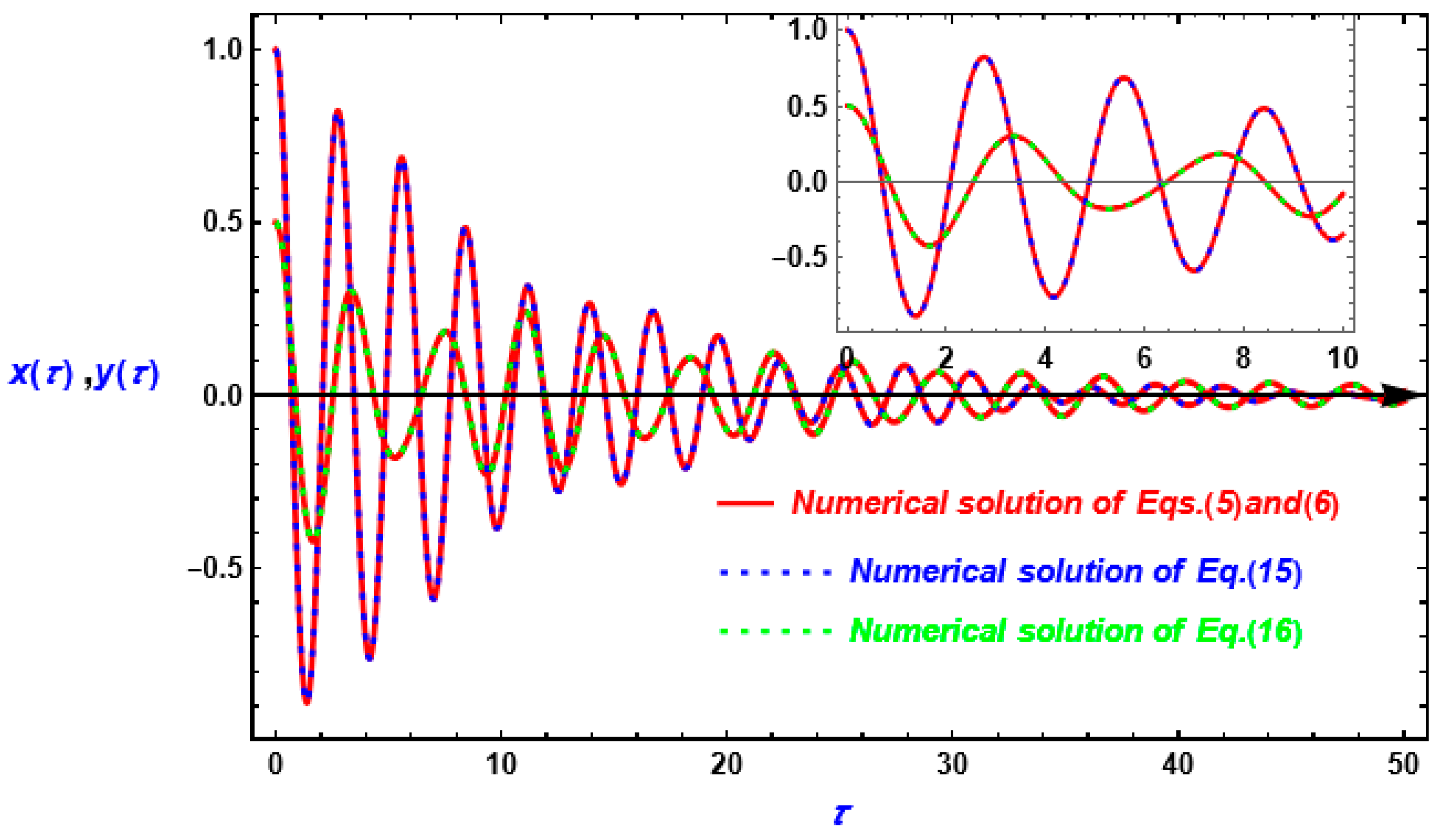
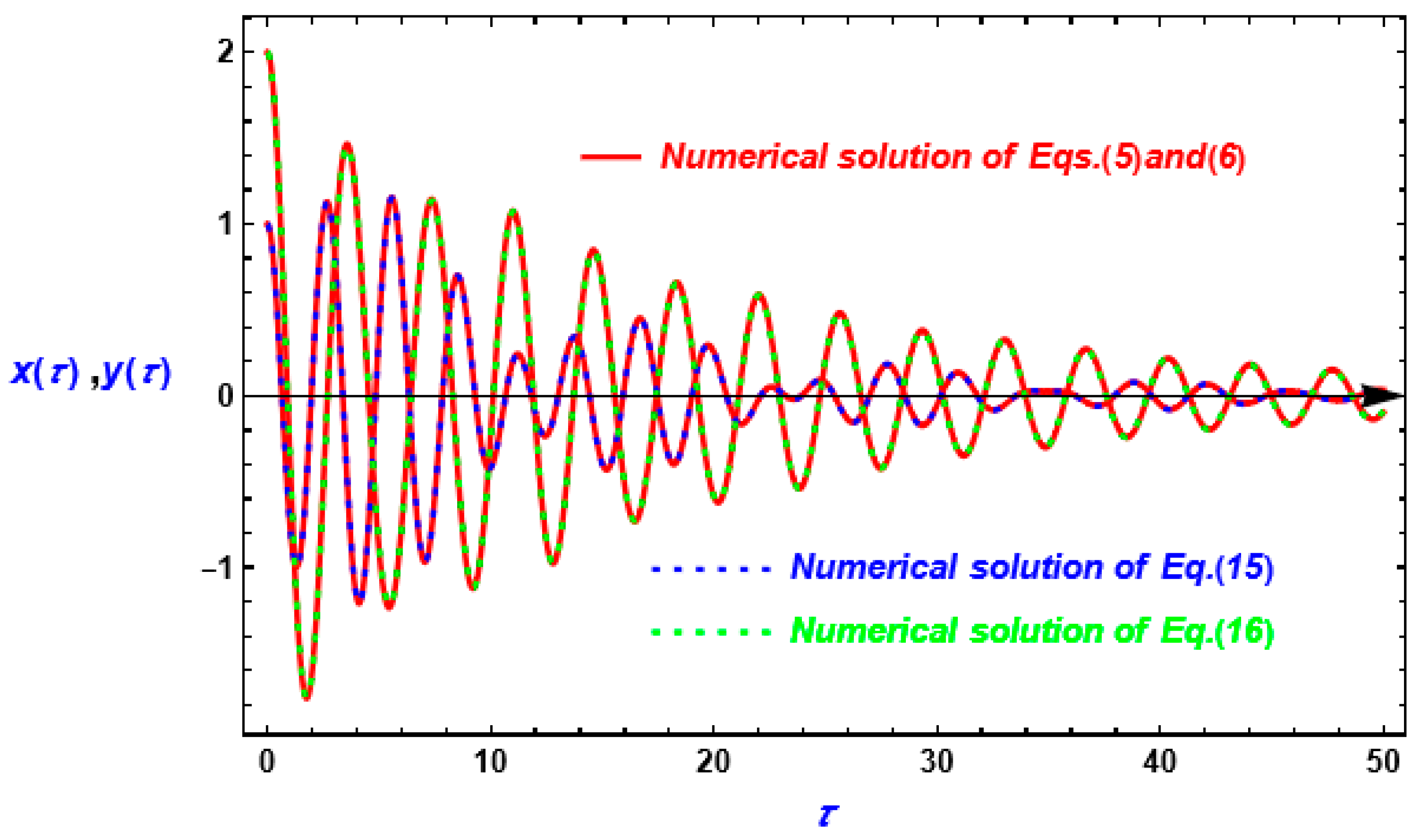
To verify that Equations (15) and (16) correctly depict the equivalent linearized version of the original nonlinear system given in Equations (5) and (6), numerical validation is performed. The suggested method is strengthened by these numerical comparisons, which also offer crucial validation for the procedure of converting a nonlinear system into its linear equivalent. The numerical responses of the nonlinear system and its corresponding linearized counterpart provided by Equations (15) and (16) are shown in Figure 2 and Figure 3 under the initial conditions specified in Equation (7). This comparison evaluates how well the transformation replicates the dynamic behavior of the system using the given numerical parameters. The outcomes confirm the linearized model’s usefulness as an analogous representation and show how well it captures the essential characteristics of the nonlinear system.

$$A=1, B=0.5, {\mu }_1=0.2, {\mu }_2=0.1, a_1=5, a_2=3, a_3=0.5, a_4=0.3,$$

$$q_1=q_2=q_3=q_4=1, {\omega }_0=5,{\gamma }_1={\gamma }_2={\eta }_1={\eta }_2=0.01.$$

These numerical values were selected to facilitate a realistic comparison between the nonlinear system and its linearized models, ensuring that both stability and dynamic responses can be properly assessed under identical initial conditions. The results indicate strong agreement between the nonlinear and linearized systems, suggesting that the linearization transformation efficiently captures the original system’s fundamental characteristics. The analysis presented indicates that the transformed model maintains accuracy in capturing the system dynamics, even with increased initial excitation amplitudes. Numerical comparisons show relative errors of 0.007746 and 0.003179 at moderate amplitudes, aligning closely between models. With higher initial amplitudes, errors rise to 0.02783 and 0.01344, yet remain small, indicating consistent preservation of essential dynamic features such as energy exchange and stability. This validates the linear approximation’s reliability in describing system behavior within the tested amplitude range, demonstrating the robustness of the proposed model.

3.1. Self-Conversion into an Autonomous System

The outcomes (15) and (16) are coupled oscillations that constitute a non-autonomous system. For the sake of mathematical simplicity [62,63], it is preferable to make it autonomous. We adopt an appropriate weight function $\chi \left(\tau \right)=\cos \left(n \tau \right)$ to renormalize the periodic function cos $\left(2{\omega }_0\tau \right)$ [64,65] to convert the aforementioned system into an autonomous system:

$$K_n({\omega }_0)={\displaystyle \frac{{\displaystyle \underset{0}{\overset{\pi /2{\omega }_0}{\int }}{\chi }^2(\tau )\hspace{0.17em}\hspace{0.17em}\cos (2{\omega }_0\tau )d\tau }\hspace{0.17em}}{{\displaystyle \underset{0}{\overset{\pi /2{\omega }_0}{\int }}{\chi }^2(\tau )\hspace{0.17em}}d\tau }}={\displaystyle \frac{n^2{\omega }_0\sin \left(\frac{n\pi }{{\omega }_0}\right)}{\left({\omega }_0^2-n^2\right)\left(n\pi +{\omega }_0\sin \left(\frac{n\pi }{{\omega }_0}\right)\right)}};\hspace{0.17em}\hspace{0.17em}\hspace{0.17em}n=1,2,3,\dots$$

(17)

The non-autonomous Equations (15) and (16) are reformulated as an autonomous system through the application of the Equation (17), as follows:

$$x^{″}+{\mu }_1{x}^{\prime }+\left(a_1+{\varpi }_1^2+q_1{K}_n({\omega }_0)\right)x+\left(a_3+{\varpi }_3^2+q_3{K}_n({\omega }_0)\right)y=0,$$

(18)

$$y^{″}+{\mu }_2{y}^{\prime }+\left(a_2+{\varpi }_2^2+q_2{K}_n({\omega }_0)\right)y+\left(a_4+{\varpi }_4^2+q_4{K}_n({\omega }_0)\right)x=0.$$

(19)

It is possible to examine the following simple system’s form:

$$x^{″}+{\mu }_1{x}^{\prime }+{\sigma }_1^{2}x+{\sigma }_3^{2}y=0,$$

(20)

$$y^{″}+{\mu }_2{y}^{\prime }+{\sigma }_2^{2}y+{\sigma }_4^{2}x=0,$$

(21)

where

$${\sigma }_j^2=a_j+{\varpi }_j^2+q_j{K}_n({\omega }_0);\hspace{0.17em}\hspace{0.17em}\hspace{0.17em}j=1:4.$$

(22)

The revised Equations (20) and (21) make it much easier to analyze the system’s dynamic behavior by removing the challenges associated with changing coefficients. This transformation simplifies the governing equations, enabling a more thorough analysis of key phenomena such as resonance, balance, and matched nonlinear interactions. By reducing analytical complexity, it becomes easier to apply advanced solution approaches, allowing for more precise characterization of the dynamic response and a better understanding of the system’s balance and performance.

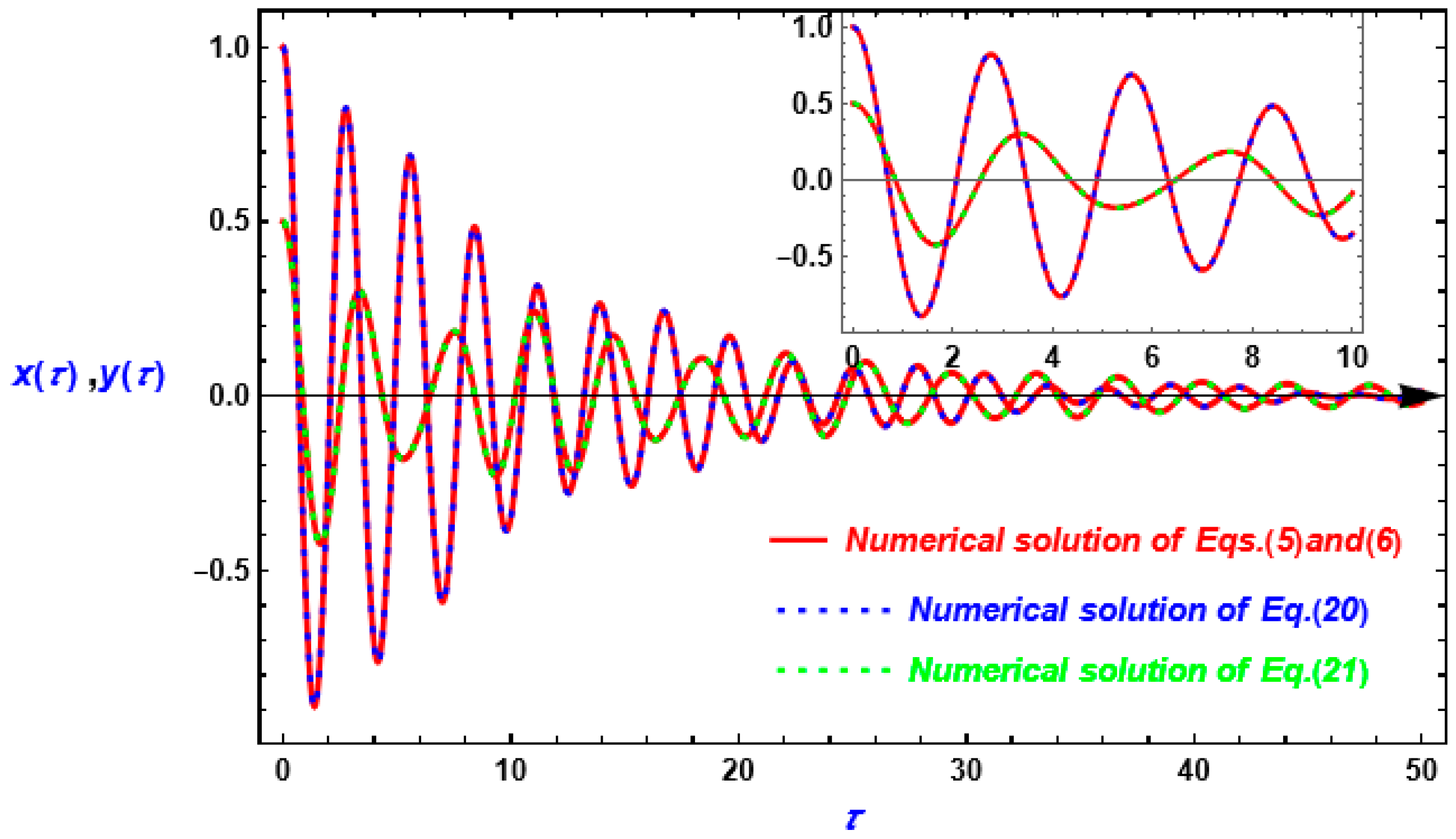
Numerical comparisons strongly support the proposed methodology and provide crucial validation for converting a non-autonomous system into an autonomous one. Figure 4 depicts the numerical solutions of the original non-autonomous system, dictated by Equations (5) and (6), as solid red curves, and the solutions of the converted autonomous system, defined by Equations (20) and (21), as dashed blue and green trajectories. The strong similarity between the two sets of solutions suggests that the autonomous formulation accurately replicates the dynamics of the non-autonomous system. The relative errors of 0.01192 and 0.002355 confirm the transformation’s great precision. These findings show that the suggested method provides a precise approximation of the actual system, outperforming perturbation strategies confined to small-amplitude responses. The comparison uses the numerical parameters indicated in Figure 2 to determine if the applied transformation accurately depicts the genuine physical response of the original system. From an engineering standpoint, the transformation can be described as the replacement of an explicitly time-dependent excitation (non-autonomous system) with an equivalent internal dynamical mechanism (autonomous system) that reproduces the same energy exchange, coupling, and stability characteristics. The simulated results reveal that major engineering performance metrics like vibration amplitudes, dominant frequencies, phase trajectories, and stability boundaries remain mostly unaffected after transformation. This shows that the autonomous formulation retains the effective stiffness, inertia, damping, and coupling effects that govern the system’s motion. In physical terms, the transformed system reacts to excitations in a way that is dynamically indistinguishable from the original time-driven system. This equivalency has practical engineering implications. It means that the autonomous representation can be utilized to correctly study resonance, bifurcation behavior, and long-term stability with traditional nonlinear dynamics methods while maintaining physical realism. As a result, the transformation creates a stable and physically consistent model that facilitates analysis while remaining true to the original non-autonomous dynamics.

3.2. Transformation of the Fractional Derivative into the Traditional Derivative

Fractal derivatives are mapped into corresponding classical derivatives using El-Dib’s fractal transformation, which preserves the fundamental scale-dependent and memory properties of the original fractal model while enabling the use of well-known analytical methods. This transformation greatly simplifies stability and frequency calculations by providing a physically consistent link between fractal dynamics and conventional vibration theory. In terms of limits, the transformation works best with smoothly shifting responses and weak to moderate fractality. Higher-order corrections or direct numerical treatment of the initial fractal model may be necessary for systems with extremely strong fractal effects, discontinuities, or substantially non-smooth dynamics. The updated manuscript now includes these clarified issues.

To convert a fractional-order derivative into an equivalent integer-order derivative, El-Dib devised a fractal time-scaling technique. Systems with intrinsic fractional dynamics, such as oscillatory, chaotic, or nonlinear systems, benefit greatly from this method. Fractional derivatives are transformed into classical derivatives in the new time scale by rescaling time using a fractal exponent, τ = t^α. This transformation permits the application of common analytical and numerical techniques while preserving the fundamental dynamics of the system. It is worth noting that converting the fractal derivative into an integer-order derivative simplifies the fractal linear coupling system (20) and (21), which is beneficial in the fractal variable τ = t^α. Following the latest publications [21,22,23], where this claim was made, is a wise approach.

$${\displaystyle \frac{d..}{d\tau }}={\displaystyle \frac{d..}{d{t}^{\alpha }}}={\delta }^{\alpha -1}\sin \left(\frac{1}{2}\pi \alpha \right)\hspace{0.17em}\hspace{0.17em}{\displaystyle \frac{d..}{dt}}+{\delta }^{\alpha }\cos \left(\frac{1}{2}\pi \alpha \right)\hspace{0.17em}\hspace{0.17em}..,$$

(23)

where $\delta$ is a real parameter that depends on the fractal order$, \alpha$. The following expression is sufficient:

$${\displaystyle \frac{d..}{d{t}^{2\alpha }}}=\left({\delta }^{2\alpha -2}{\sin }^2\left(\frac{1}{2}\pi \alpha \right){\displaystyle \frac{d^2..}{d{t}^2}}+2{\delta }^{2\alpha -1}\sin \left(\frac{1}{2}\pi \alpha \right)\cos \left(\frac{1}{2}\pi \alpha \right){\displaystyle \frac{d..}{dt}}+{\delta }^{2\alpha }{\cos }^2\left(\frac{1}{2}\pi \alpha \right)..\right).$$

(24)

By establishing a link between fractal and conventional derivatives, these transformations enable the use of analytical solutions. Combining (23) and (24) with (20) and (21) results in

$$\ddot{x}+R_1\dot{x}+P_{1}x\hspace{0.17em}\hspace{0.17em}+P_{3}y=0,$$

(25)

$$\ddot{y}+R_2\dot{y}\hspace{0.17em}\hspace{0.17em}+P_{2}y+P_{4}x=0,$$

(26)

where

$$\begin{array}{l}{R}_j={\displaystyle \frac{1}{{\delta }^{\alpha -1}\sin \left(\frac{1}{2}\pi \alpha \right)}}\left({\mu }_j+2{\delta }^{\alpha }\cos \left(\frac{1}{2}\pi \alpha \right)\right);\hspace{0.17em}\hspace{0.17em}j=1,2\\ P_j={\displaystyle \frac{1}{{\delta }^{2\alpha -2}{\sin }^2\left(\frac{1}{2}\pi \alpha \right)}}\left({\delta }^{2\alpha }{\cos }^2\left(\frac{1}{2}\pi \alpha \right)+{\mu }_j{\delta }^{\alpha }\cos \left(\frac{1}{2}\pi \alpha \right)+{\sigma }_j^2\right),\\ P_{j+2}={\displaystyle \frac{{\sigma }_{j+2}^2}{{\delta }^{2\alpha -2}{\sin }^2\left(\frac{1}{2}\pi \alpha \right)}}.\end{array}$$

(27)

Additionally, the initial conditions mentioned in (3) will change to

$$x(0)=A, \dot{x}\left(0\right)=-A\delta \cot \left(\frac{1}{2}\pi \alpha \right) \mathrm{and} y(0)=B, \dot{y}(0)-B\delta \cot \left(\frac{1}{2}\pi \alpha \right).$$

(28)

The fractal system (25) and (26) is characterized by the fractal dimension α and the unknown fractalized parameter δ. The system’s development is based on El-Dib’s metamorphosis, and it is noted that the present fractal system is related to the full initial conditions in (28), whereas the original fractal system was connected by semi-initial conditions given in (7). The entire structure (23) is the basis for these foundations. Determining the unknown fractalized parameter is necessary to identify a fractal system that depends on the physical properties of the original system rather than on the dimension parameter directly. This will be covered in the next subsection.

3.3. Established the Fractal System Dependence on the Physical Parameters

Since the original system of Equations (20) and (21) corresponds to the outcome fractal system of Equations (25) and (26), their frequencies are the same, meaning that the corresponding natural frequencies in both systems are the same. The comparison to these frequencies results in the following equalities because there are two major and secondary frequencies:

For the major frequencies

$${\sigma }_1^2\equiv {\displaystyle \frac{1}{{\delta }^{2\alpha -2}{\sin }^2\left(\frac{1}{2}\pi \alpha \right)}}\left({\delta }^{2\alpha }{\cos }^2\left(\frac{1}{2}\pi \alpha \right)+{\mu }_1{\delta }^{\alpha }\cos \left(\frac{1}{2}\pi \alpha \right)+{\sigma }_1^2\right),$$

(29)

$${\sigma }_2^2\equiv {\displaystyle \frac{1}{{\delta }^{2\alpha -2}{\sin }^2\left(\frac{1}{2}\pi \alpha \right)}}\left({\delta }^{2\alpha }{\cos }^2\left(\frac{1}{2}\pi \alpha \right)+{\mu }_2{\delta }^{\alpha }\cos \left(\frac{1}{2}\pi \alpha \right)+{\sigma }_2^2\right).$$

(30)

For the secondary frequencies

$${\sigma }_3^2\equiv {\displaystyle \frac{{\sigma }_3^2}{{\delta }^{2\alpha -2}{\sin }^2\left(\frac{1}{2}\pi \alpha \right)}},$$

(31)

$${\sigma }_4^2\equiv {\displaystyle \frac{{\sigma }_4^2}{{\delta }^{2\alpha -2}{\sin }^2\left(\frac{1}{2}\pi \alpha \right)}}.$$

(32)

The comparison of secondary frequencies (31) and (32) yields the following equality:

$${\delta }^{2\alpha -2}{\sin }^2\left(\frac{1}{2}\pi \alpha \right)=1.$$

(33)

This equation can be satisfied only when $\alpha =1$, which can be ignored because $\alpha <1$ according to the hypothesis. The comparison of the major frequencies that are cited in Equations (29) and (30) reads as

$${\delta }^{2\alpha -2}{\sin }^2\left(\frac{1}{2}\pi \alpha \right)={\displaystyle \frac{{\delta }^{2\alpha }{\cos }^2\left(\frac{1}{2}\pi \alpha \right)+{\mu }_2{\delta }^{\alpha }\cos \left(\frac{1}{2}\pi \alpha \right)+{\sigma }_2^2}{{\sigma }_2^2}}={\displaystyle \frac{{\delta }^{2\alpha }{\cos }^2\left(\frac{1}{2}\pi \alpha \right)+{\mu }_1{\delta }^{\alpha }\cos \left(\frac{1}{2}\pi \alpha \right)+{\sigma }_1^2}{{\sigma }_1^2}}.$$

(34)

Keeping in mind that $\alpha \ne 1$, this comparison leads to the following equation:

$${\delta }^{\alpha }\cos \left(\frac{1}{2}\pi \alpha \right)={\displaystyle \frac{{\sigma }_2^2{\mu }_1-{\sigma }_1^2{\mu }_2}{{\sigma }_1^2-{\sigma }_2^2}}.$$

(35)

Combining Equation (35) with Equation (34) yields

$${\delta }^{\alpha -1}\sin \left(\frac{1}{2}\pi \alpha \right)=\sqrt{1+{\displaystyle \frac{{\mu }_2^2{\sigma }_1^2+{\mu }_1^2{\sigma }_2^2-{\mu }_1{\mu }_2\left({\sigma }_1^2+{\sigma }_2^2\right)}{{\left({\sigma }_1^2-{\sigma }_2^2\right)}^2}}}.$$

(36)

These findings provide us with the unknown fractalizing parameter δ, which is given by

$${\delta }^2={\displaystyle \frac{{\left({\sigma }_2^2{\mu }_1-{\sigma }_1^2{\mu }_2\right)}^2}{{\mu }_2^2{\sigma }_1^2+{\mu }_1^2{\sigma }_2^2-{\mu }_1{\mu }_2\left({\sigma }_1^2+{\sigma }_2^2\right)+{\left({\sigma }_1^2-{\sigma }_2^2\right)}^2}}{\tan }^2\left(\frac{1}{2}\pi \alpha \right).$$

(37)

The fractal systems (25) and (26) have the following simplified form, which is independent of the parameters α and δ, based on the results mentioned in Equations (35) and (36):

$$\ddot{x}+{\lambda }_1\dot{x}+{\sigma }_1^{2}x+{\rho }_1^{2}y=0,$$

(38)

$$\ddot{y}+{\lambda }_2\dot{y}\hspace{0.17em}+{\sigma }_2^{2}y+{\rho }_2^{2}x=0,$$

(39)

where

$${\lambda }_1=\sqrt{{\displaystyle \frac{{\left({\mu }_1\left({\sigma }_1^2+{\sigma }_2^2\right)-2{\sigma }_1^2{\mu }_2\right)}^2}{{\mu }_2^2{\sigma }_1^2+{\mu }_1^2{\sigma }_2^2-{\mu }_1{\mu }_2\left({\sigma }_1^2+{\sigma }_2^2\right)+{\left({\sigma }_1^2-{\sigma }_2^2\right)}^2}}},$$

(40)

$${\lambda }_2=\sqrt{{\displaystyle \frac{{\left({\mu }_2\left({\sigma }_1^2+{\sigma }_2^2\right)-2{\sigma }_2^2{\mu }_1\right)}^2}{{\mu }_2^2{\sigma }_1^2+{\mu }_1^2{\sigma }_2^2-{\mu }_1{\mu }_2\left({\sigma }_1^2+{\sigma }_2^2\right)+{\left({\sigma }_1^2-{\sigma }_2^2\right)}^2}}},$$

(41)

$${\rho }_1^2={\displaystyle \frac{{\sigma }_3^2{\left({\sigma }_1^2-{\sigma }_2^2\right)}^2}{{\mu }_2^2{\sigma }_1^2+{\mu }_1^2{\sigma }_2^2-{\mu }_1{\mu }_2\left({\sigma }_1^2+{\sigma }_2^2\right)+{\left({\sigma }_1^2-{\sigma }_2^2\right)}^2}},$$

(42)

$${\rho }_2^2={\displaystyle \frac{{\sigma }_4^2{\left({\sigma }_1^2-{\sigma }_2^2\right)}^2}{{\mu }_2^2{\sigma }_1^2+{\mu }_1^2{\sigma }_2^2-{\mu }_1{\mu }_2\left({\sigma }_1^2+{\sigma }_2^2\right)+{\left({\sigma }_1^2-{\sigma }_2^2\right)}^2}}.$$

(43)

In this state, the initial conditions in (28) become

$$x(0)=A, \dot{x}\left(0\right)={\displaystyle \frac{A\left({\sigma }_1^2{\mu }_2-{\sigma }_2^2{\mu }_1\right)}{{\sigma }_1^2-{\sigma }_2^2}} \mathrm{and} y(0)=B, \dot{y}(0)={\displaystyle \frac{B\left({\sigma }_1^2{\mu }_2-{\sigma }_2^2{\mu }_1\right)}{{\sigma }_1^2-{\sigma }_2^2}}.$$

(44)

4. The Scheme for Converting Coupled Equations (38) and (39) into Decoupled Equations

Because the dynamics of the variables affect one another, many nonlinear dynamical systems comprise two or more coupled equations that are challenging to solve analytically. Common techniques, like modal decomposition, may call on special-case presumptions like weak coupling, symmetry, or equal frequencies. In order to represent the dominant dynamics of one subsystem (or one degree of freedom) in the linked system, two unique independent time variables are introduced. The derivatives are then adjusted when the coupled equations are rewritten in terms of these additional variables. This essentially lowers the coupling since each original equation may be represented mostly in terms of a single independent variable. The equations are now decoupled, making it possible to solve each one separately. This approach is appropriate for strongly coupled systems since it does not rely on special-case assumptions like equal frequencies or linear coupling. Additionally, it makes analysis, simulation, stability, and resonance investigations easier and does away with the need for symmetry or resonance conditions.

A streamlined framework for analyzing the system’s dynamics is provided by the decoupled equations. The coupled system’s complexity can be reduced by separating the variables x(t) and y(t), enabling a simpler investigation of stability, resonance, and other dynamic characteristics. Introducing new Lindstedt-Poincaré transformations [65,66] is a more practical method that is defined as

$$\xi ={\Omega }_{1}t, \mathrm{and} \zeta ={\Omega }_{2}t.$$

(45)

The derivatives will be changed in accordance with the previously mentioned new variables.

$${\displaystyle \frac{d..}{dt}}={\displaystyle \frac{d..}{d\xi }}{\displaystyle \frac{d\xi }{dt}}+{\displaystyle \frac{d..}{d\zeta }}{\displaystyle \frac{d\zeta }{dt}}={\Omega }_1{\displaystyle \frac{d..}{d\xi }}+{\Omega }_2{\displaystyle \frac{d..}{d\zeta }},$$

(46)

$${\displaystyle \frac{d^2..}{d{t}^2}}={\Omega }_1^2{\displaystyle \frac{d^2..}{d{\xi }^2}}+2{\Omega }_1{\Omega }_2{\displaystyle \frac{d^2..}{d\xi d\zeta }}+{\Omega }_2^2{\displaystyle \frac{d^2..}{d{\zeta }^2}}.$$

(47)

The system’s variables will change from $x(t)\hspace{0.17em}\mathrm{and}\hspace{0.17em}y(t)$ to $x(\xi )\hspace{0.17em}\mathrm{and}\hspace{0.17em}y(\zeta )$ based on these modifications (45) so that the set of Equations (38) and (39) changes to

$$\left({\Omega }_1^2{\displaystyle \frac{d^2}{d{\xi }^2}}+{\Omega }_1{\lambda }_1{\displaystyle \frac{d}{d\xi }}+{\sigma }_1^2\right)x\left(\xi \right)+{\rho }_1^{2}y\left(\zeta \right)=0,$$

(48)

$$\left({\Omega }_2^2{\displaystyle \frac{d^2}{d{\zeta }^2}}+{\Omega }_2{\lambda }_2{\displaystyle \frac{d}{d\zeta }}+{\sigma }_2^2\right)y\left(\zeta \right)+{\rho }_2^{2}x\left(\xi \right)=0.$$

(49)

These equations can be decoupled by removing the variable $y\left(\zeta \right)$ from Equation (48) using Equation (49), which yields the following:

$${\Omega }_1^2{\displaystyle \frac{d^{2}x}{d{\xi }^2}}+{\Omega }_1{\lambda }_1{\displaystyle \frac{dx}{d\xi }}+{\displaystyle \frac{1}{{\sigma }_2^2}}\left({\sigma }_1^2{\sigma }_2^2-{\rho }_1^2{\rho }_2^2\right)x\left(\xi \right)=0.$$

(50)

Correspondingly, leads to the following equation

$${\Omega }_2^2{\displaystyle \frac{d^{2}y}{d{\zeta }^2}}+{\Omega }_2{\lambda }_2{\displaystyle \frac{dy}{d\zeta }}+{\displaystyle \frac{1}{{\sigma }_1^2}}\left({\sigma }_1^2{\sigma }_2^2-{\rho }_1^2{\rho }_2^2\right)y\left(\zeta \right)=0.$$

(51)

Reverting to the original variable t in Equations (50) and (51) leads to the following:

$$\ddot{x}+{\lambda }_1\dot{x}+{\displaystyle \frac{1}{{\sigma }_2^2}}\left({\sigma }_1^2{\sigma }_2^2-{\rho }_1^2{\rho }_2^2\right)x(t)=0,$$

(52)

$$\ddot{y}+{\lambda }_2\dot{y}+{\displaystyle \frac{1}{{\sigma }_1^2}}\left({\sigma }_1^2{\sigma }_2^2-{\rho }_1^2{\rho }_2^2\right)y(t)=0.$$

(53)

Based on the damped linear harmonic equations above, the total frequencies Ω₁ and Ω₂ can be expressed as follows:

$${\Omega }_1^2={\displaystyle \frac{1}{{\sigma }_2^2}}\left({\sigma }_1^2{\sigma }_2^2-{\rho }_1^2{\rho }_2^2\right)-{\displaystyle \frac{1}{4}}{\lambda }_1^2,$$

(54)

$${\Omega }_2^2={\displaystyle \frac{1}{{\sigma }_1^2}}\left({\sigma }_1^2{\sigma }_2^2-{\rho }_1^2{\rho }_2^2\right)-{\displaystyle \frac{1}{4}}{\lambda }_2^2.$$

(55)

Because stability requires ${\Omega }_1^2$ > 0 and ${\Omega }_{2 }^2$ > 0, along with ${\lambda }_1>0$ and ${\lambda }_2>0$, the system remains stable when

$${\displaystyle \frac{1}{{\sigma }_2^2}}\left({\sigma }_1^2{\sigma }_2^2-{\rho }_1^2{\rho }_2^2\right)-{\displaystyle \frac{1}{4}}{\lambda }_1^2>0, \mathrm{and} {\displaystyle \frac{1}{{\sigma }_1^2}}\left({\sigma }_1^2{\sigma }_2^2-{\rho }_1^2{\rho }_2^2\right)-{\displaystyle \frac{1}{4}}{\lambda }_2^2>0.$$

(56)

Because of the initial conditions mentioned in (44), the solutions to Equations (52) and (53) have the following form:

$$x(t)=A{e}^{-{\displaystyle \frac{1}{2}}{\lambda }_{1}t}\left(\cos {\Omega }_{1}t+{\displaystyle \frac{1}{{\Omega }_1}}\left(m+{\displaystyle \frac{1}{2}}{\lambda }_1\right)\sin {\Omega }_{1}t\right),$$

(57)

$$y(t)=B{e}^{-{\displaystyle \frac{1}{2}}{\lambda }_{2}t}\left(\cos {\Omega }_{2}t+{\displaystyle \frac{1}{{\Omega }_2}}\left(m+{\displaystyle \frac{1}{2}}{\lambda }_2\right)\sin {\Omega }_{2}t\right),$$

(58)

where

$$m={\displaystyle \frac{{\sigma }_1^2{\mu }_2-{\sigma }_2^2{\mu }_1}{{\sigma }_1^2-{\sigma }_2^2}}.$$

(59)

These general solutions describe the time-dependent behavior of the variables x($t$) and y($t).$

5. Numerical Validation

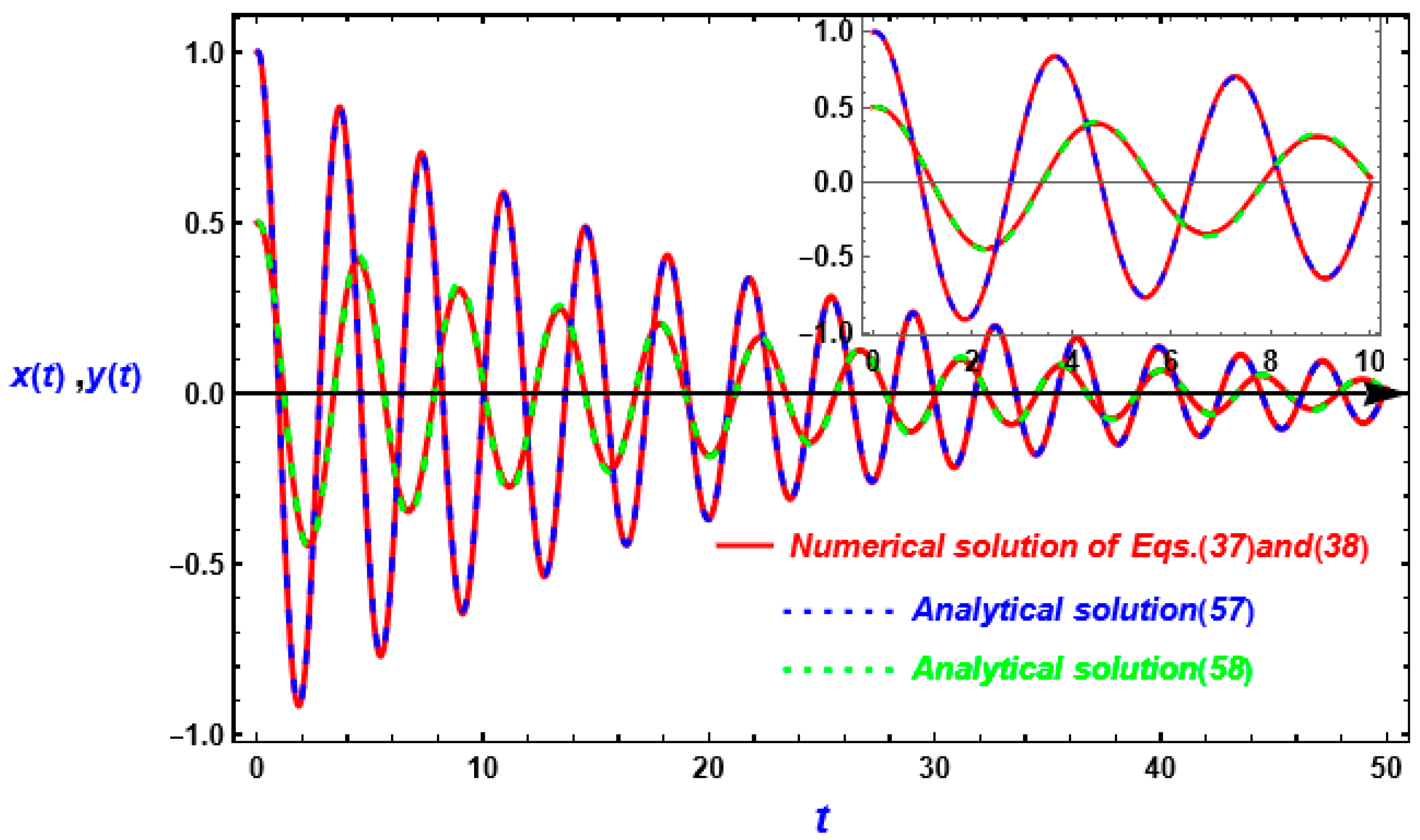
Numerical testing confirms the accuracy and reliability of the analytical solutions described by (57) and (58). Figure 5 compares the fractal system defined by Equations (38) and (39) with their analytical results in (57) and (58). Using the given parameter values, this comparison evaluates how effectively the analytical solution reflects the system’s actual dynamics. Calculations are based on the following numerical values:

$$A=1, B=0.5, {\mu }_1= {\mu }_2=0.1, a_1=2, a_2=3, a_3=0.01, a_4=0.01, q_j=1, {\omega }_0=20, {\gamma }_1={\gamma }_2={\eta }_1={\eta }_2=0.01.$$

In these computations, the major natural and secondary frequencies σ_j, which are specified in (22) have the following values: ${\sigma }_1$ = $1.4173,$ ${\sigma }_2$ = $1.73295,$ ${\sigma }_3$ = $0.13693,$ and ${\sigma }_4$ = $0.1146.$ These modified parameters allow for a more accurate assessment of the analytical solution’s validity over a wider variety of settings. The relative errors calculated for the obtained solutions demonstrate the validity of the study. Solution (57) has a relative error of 0.008771, while solution (58) has 0.02908—both are sufficiently small to confirm the high accuracy of the results. These findings indicate that the technique effectively approximates the dynamics of the non-independent system and accurately captures shooting stability transitions. Overall, the validation enhances confidence in the analytical method and its suitability for complex dynamic structures.

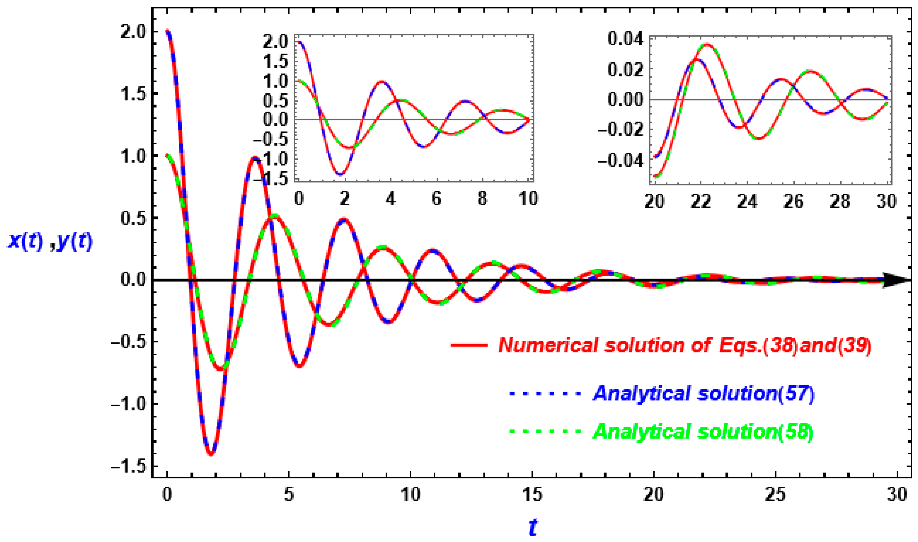
Figure 6 displays the same type of comparison given in Figure 5, using a different numerical system, $A=2, B=1, {\mu }_1= 0.2, {\mu }_2=0.1, a_1=3, a_2=2$, with the other parameters held constant. The damping parameters are altered, and the major natural frequencies are inverted. This results in σ₁ = 1.73674, σ₂ = 1.4160, σ₃ = 0.1620, and σ₄ = 0.1225, with updated damping coefficients λ₁ = 0.3946 and λ₂ = 0.2951. These changes provide a stronger damping effect, yet the analytical and numerical solutions remain closely aligned, even at high initial amplitudes, demonstrating the method’s exceptional accuracy.

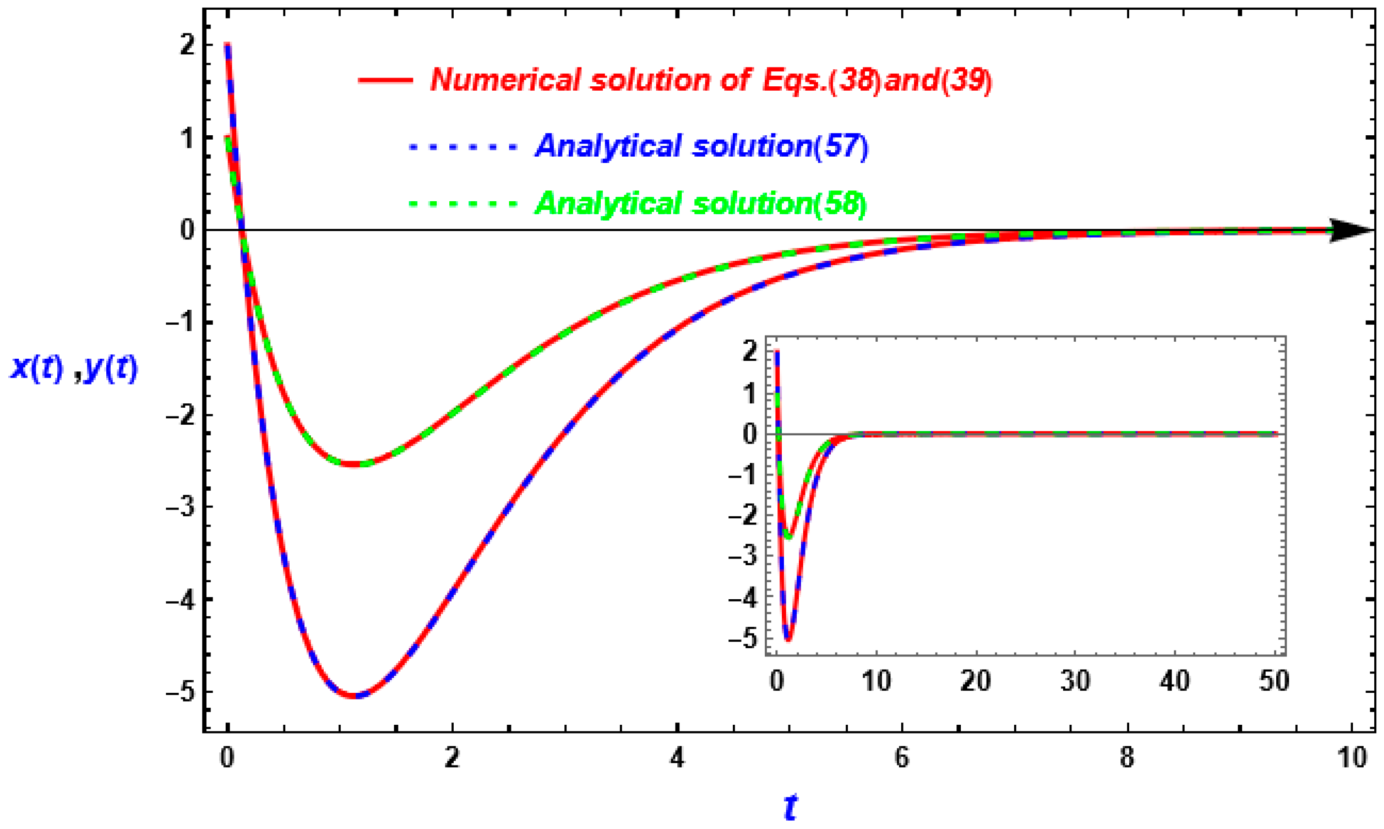
Figure 7 shows the same type of comparison as in Figure 5, however, for the resonance scenario where the two principal natural frequencies are identical, i.e., $a_1=a_2=1$, with ${\mu }_1>{\mu }_2$, while keeping the other values unchanged. The fractal effect parameter results in adjusted natural frequencies σ₁ = $1.0081$, σ₂ = $1.0025$, σ₃ = $0.5624$, and σ₄ = $0.3240$, as well as updated damping coefficients λ₁ = $2.0036$ and λ₂ = $1.9924.$ Both the adjusted major natural frequencies and the modified damping coefficients exhibit modest changes. The parameter m, which is dependent on the adjusted natural frequencies and starting damping coefficients, has a negative value of −8.8333. The graph shows that this arrangement corresponds to a perfectly damped scenario in which the system returns to equilibrium as quickly as possible without oscillations—physically representing the state where the damping is just enough to prevent oscillatory motion.

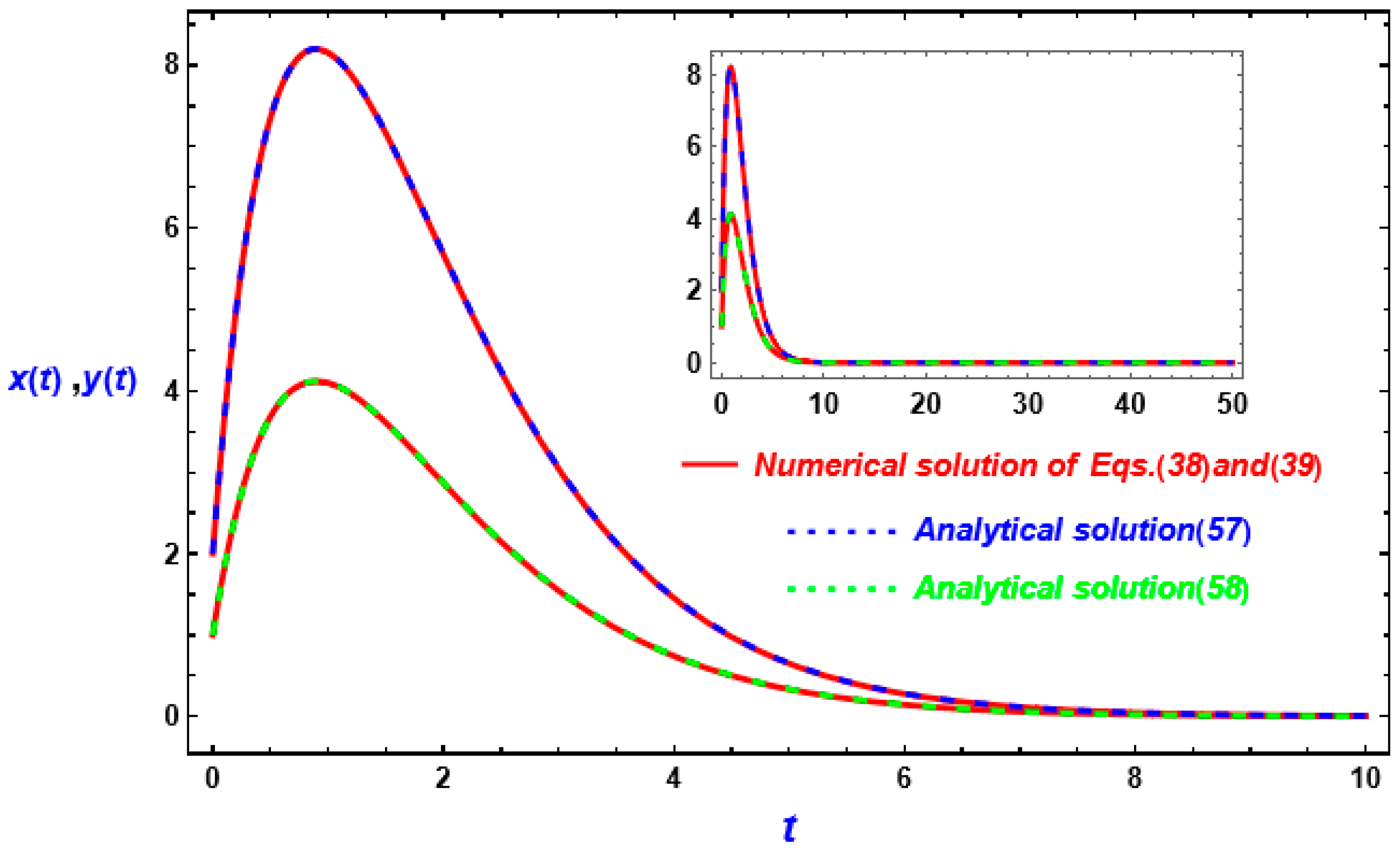
Figure 8 displays the same type of comparison as in Figure 7, representing the resonance case [65,66], where the two main natural frequencies are identical but μ₁ < μ₂, while all other parameters remain constant. The fractal influence produces modified natural frequencies and updated damping coefficients that are comparable to those shown in Figure 7, with just small differences between the two sets of values. In this calculation, the parameter m is positive, with a value of 9.1333. This positive causes an early instability phase, which is followed by a substantial damping effect that prevents oscillation. The graph shows that the amplitude initially grows dramatically—nearly four times the initial amplitude—before declining exponentially in a non-oscillatory way. This behavior reflects a thoroughly damped scenario, in which the system eventually returns to equilibrium as quickly as feasible without oscillations, physically matching the condition in which the damping is only sufficient to suppress oscillatory motion.

Identification and Detection of Stability Predictions

To find stability predictions, plot the stability criteria provided in (56) in the fractal parameter space, highlighting the stable and unstable parts of the current 2DOF system. To demonstrate stability behavior, the stability criterion (56) must be met. Individual conditions can be combined to provide a single, comprehensive stability requirement of the type

$$\varphi (A,B,{\mu }_i,a_j,q_j,{\omega }_0)>0.$$

(60)

The transition curve imposed by this condition can be found as

$$\varphi (A,B,{\mu }_i,a_j,q_j,{\omega }_0)=0.$$

(61)

The resulting stability function ϕ considers all parameters from the original conditions, where

$$\varphi =\left({\displaystyle \frac{1}{{\sigma }_2^2}}\left({\sigma }_1^2{\sigma }_2^2-{\rho }_1^2{\rho }_2^2\right)-{\displaystyle \frac{1}{4}}{\lambda }_1^2\right)\left({\displaystyle \frac{1}{{\sigma }_1^2}}\left({\sigma }_1^2{\sigma }_2^2-{\rho }_1^2{\rho }_2^2\right)-{\displaystyle \frac{1}{4}}{\lambda }_2^2\right).$$

(62)

This unified expression allows the whole stability barrier to be displayed within the impact of the fractal space, Various factors, including natural frequencies $a_j$, damping coefficients ${\mu }_j$ initial amplitudes (A and B), and excitation amplitudes q_j contribute to the stability boundary. This transition curve is critical for understanding the system’s dynamic behavior and forecasting the conditions under which the response switches between stable and unstable states. Such insights are critical for developing systems that remain stable under changing operating conditions, highlighting the regions where the system is stable. The transition curve (61), which separates the stable and unstable states, has been graphed against the excitation frequency ω₀ as shown in Figure 7, Figure 8 and Figure 9. In these figures, the numerical parameters are

$$\begin{array}{l}A=2, B=1, {\mu }_1=0.1, {\mu }_2=0.2, a_1=1.2, a_2=0.5, a_3=0.2, a_4=0.1, q_1=q_2=, q_3=q_4=Q, {\eta }_1={\eta }_2=0.01,\mathrm{and}\\ {\gamma }_1={\gamma }_2=0.01.\end{array}$$

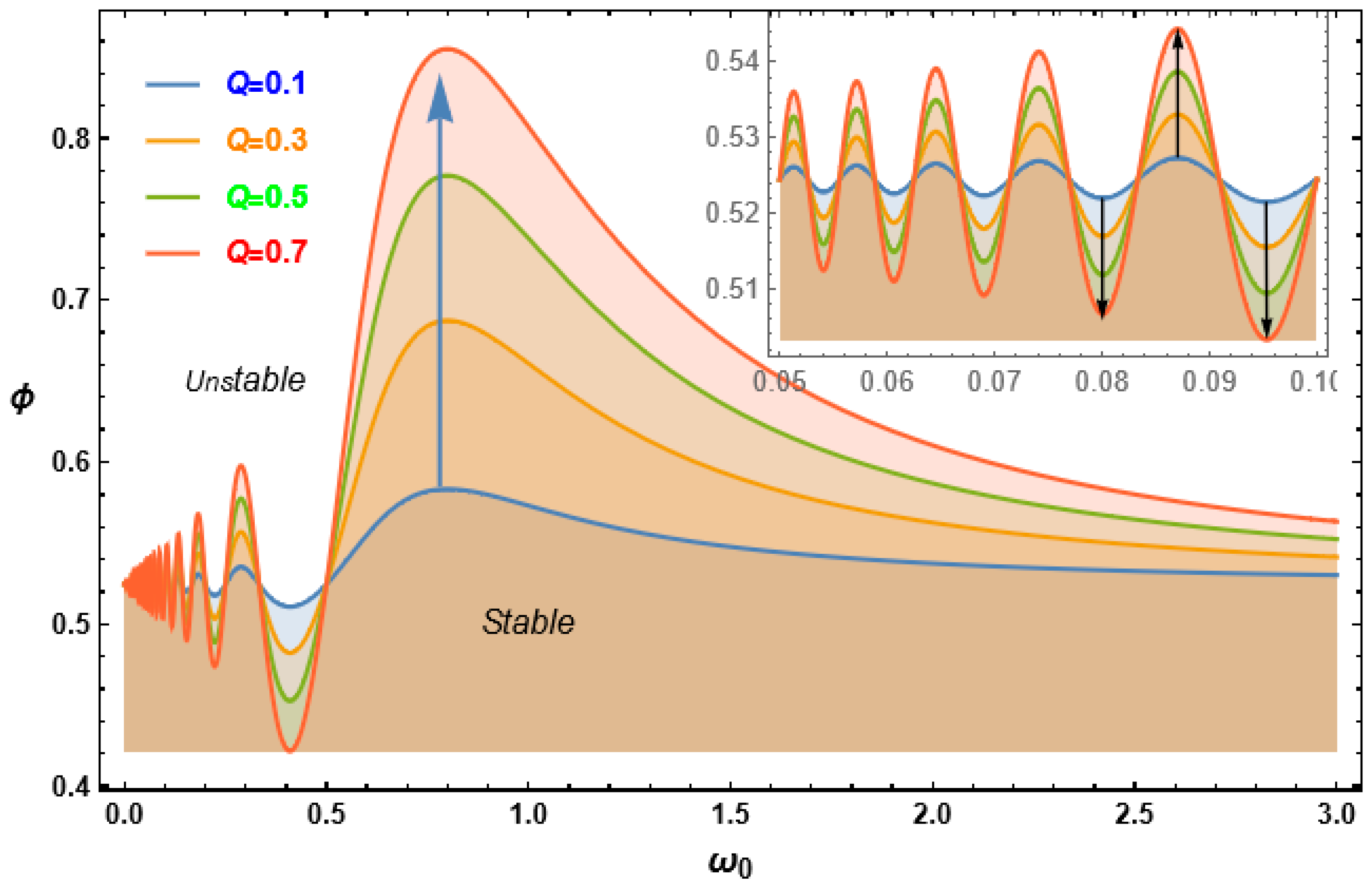
In Figure 9, the stability function ϕ has been plotted for a change in the excitation common amplitude Q (Q = $q_j, j=1:4)$. This graph illustrates how changes to the parametric excitation frequency ω₀ impact it. The graph shows the evolution of the stability boundaries as the excitation amplitude Q changes, with ω₀ ranging from 0 to 3. This graph uses a shorter variant (ω₀ = 0.05 to ω₀ = 0.1) to illustrate the finer oscillatory functions of the stability barrier at lower frequencies. Smaller ω₀ values result in more powerful oscillatory behavior at the stability limit, indicating more sensitivity in this area. The balance maps indicate that ω₀ versions have a significant impact on the transition between stable and volatile zones. A prominent peak of stability is seen near ω₀ = 1, which is referred to as extra because the excitation amplitude Q increases. These findings highlight the system’s extreme sensitivity to excitation frequency and amplitude, with ω₀ playing an essential role in determining the stability landscape. Understanding this behavior is vital for effectively anticipating and dealing with the dynamics of connected oscillatory structures. The findings have important implications for designing and improving systems in engineering, vibration control, and applied physics, all of which require precise dynamic balance treatment.

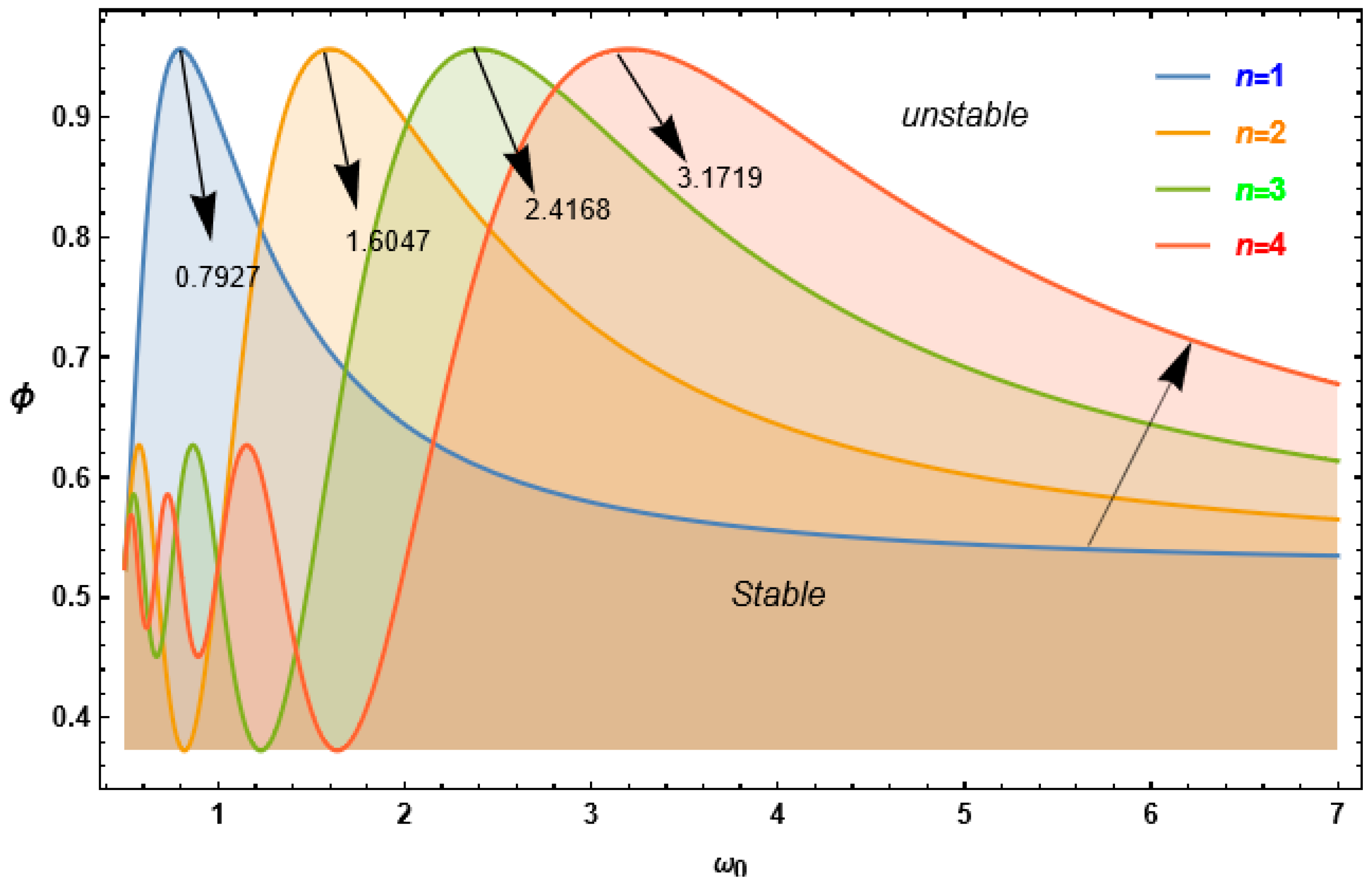
Figure 10 is plotted similarly to Figure 9, with a common amplitude of Q = 1. In this case, variation is introduced through the counter. As shown in the graph, increasing n has a significant effect on the position of the maximum stable point, which gradually shifts towards higher values of the parameter ω₀. The graph shows that the stable region grows larger as the counter n increases. Higher values of n increase the parameter space that the system can maintain stable motion in. This behavior shows that the counter has a stabilizing effect on system dynamics, boosting the stability boundary’s robustness as it develops.

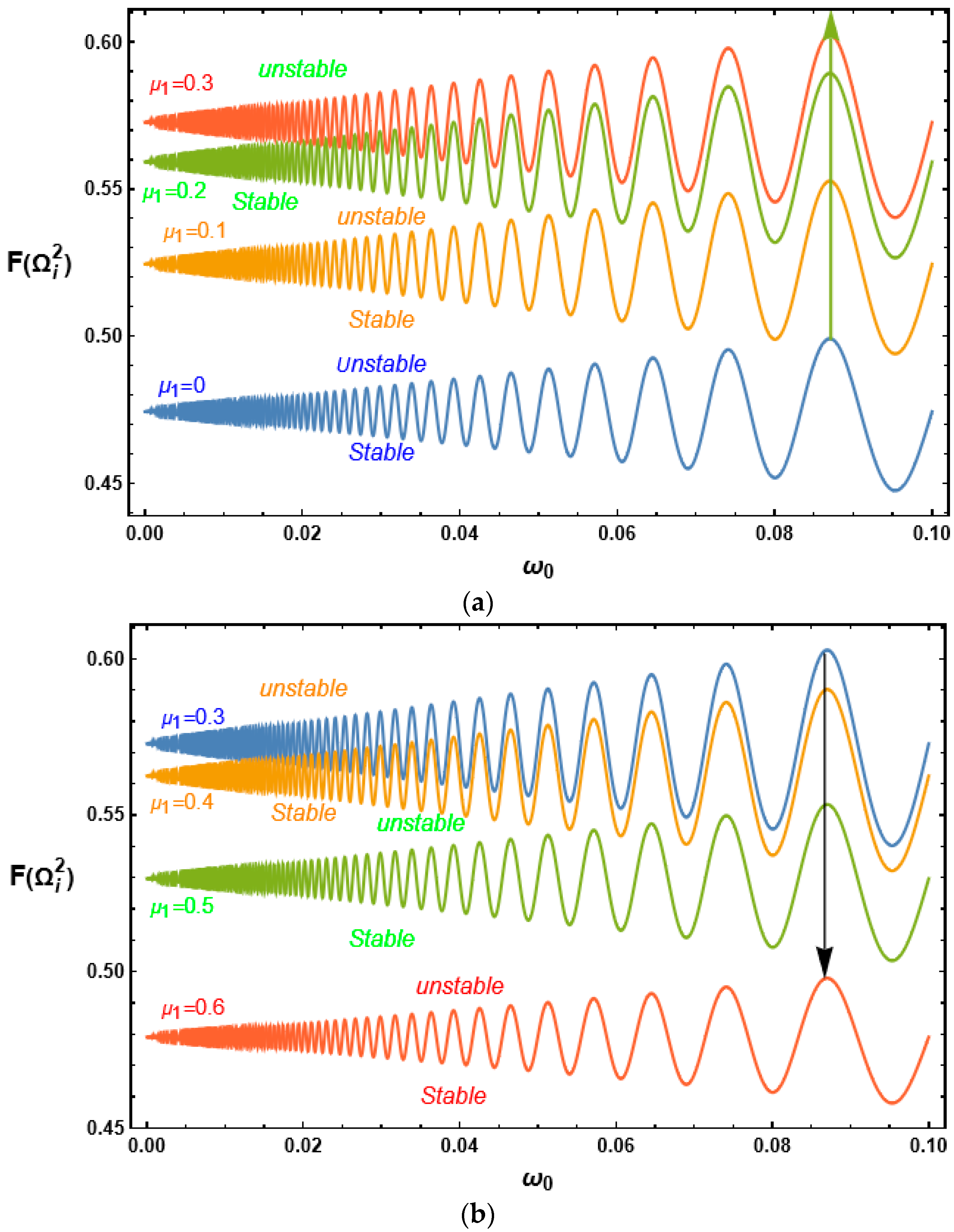
Figure 11a,b demonstrate how damping coefficients influence stability behavior. The graphs depict the impact of the damping parameter μ₁. The data indicate two distinct roles for μ₁ based on the breadth of variance. Figure 11a shows the behavior of μ₁ increasing from 0 to 0.3. Increasing μ₁ during this time causes the transition curve to go upward, enlarging the stable region and boosting overall system stability. However, increasing μ₁ over 0.3 has the opposite effect, as seen in Figure 11b. In this range (μ₁ = 0.3 to μ₁ = 0.6), increasing μ₁ shifts the transition curve downward, resulting in a smaller stable region. As a result, the system becomes unstable.

6. Conclusions

This research examines the fractal dynamics and stability of nonlinear oscillatory systems with two degrees of freedom and variable stiffness, focusing on fractal Mathieu–Duffing oscillators that arise in many practical engineering and physical applications. Micro- and nanomechanical resonators, composite and viscoelastic materials, vibration absorbers, and parametrically excited mechanical components are examples of real structures and devices that rely on material heterogeneity, memory effects, and scale-dependent behavior. From an engineering standpoint, the proposed transformation paradigm enables more precise prediction of natural frequencies and stability limits by explicitly accounting for both parametric excitation and nonlinear stiffness. This is critical in applications such as rotating machinery, MEMS devices, and structural vibration control, where small changes in excitation or stiffness can lead to instability or resonance. By translating the original non-autonomous, nonlinear model into an analogous autonomous form, the analysis is greatly simplified while preserving the system’s key physical characteristics. The nonlinear dynamics are efficiently linearized using a mean-square approximation technique, which retains the major energy exchange processes between modes. This enables the analysis of key physical phenomena, such as mode coupling, internal resonance, mode switching, and power transfer across subsystems, using tractable analytical methods. These characteristics are especially important in multi-degree-of-freedom engineering systems, where coupled vibrations can significantly impact performance, fatigue, and stability. To establish consistency with classical vibration analysis, a two-scale approach is used, mimicking existing perturbation methods but extending them to fractal and parametrically excited systems. Fractal transformations are used to convert fractal derivatives into corresponding classical derivatives, allowing standard analytical techniques to be applied while maintaining the physical interpretation associated with fractal dynamics. Furthermore, Lindstedt-Poincaré transformations with two independent temporal variables are used to decouple the interconnected linear fractal system, resulting in simpler governing equations that are nevertheless physically relevant. The findings show that reducing the fractal dimension improves overall system stability, emphasizing the stabilizing role of fractal features such as memory and scale-dependent damping. This discovery has practical significance for engineering design, implying that tweaking fractal or fractional parameters might be utilized as a passive method to reduce instability and vibrations. Finally, the excellent agreement between analytical approximations and numerical simulations justifies the proposed methodology, yielding a closed-form analytical solution for the 2DOF system’s linear autonomous representation. Overall, the research illustrates how system characteristics affect dynamic stability and demonstrates the efficacy of the suggested analytical framework for complex engineering oscillators.

Future research should focus on higher-order, multi-degree-of-freedom fractal systems to investigate complex modal interactions and stability phenomena, particularly under strong nonlinearities. It could also incorporate external disturbances and stochastic effects to mimic real-world engineering scenarios, such as in MEMS devices and smart structures, with experimental validation. The proposed methodology may enhance both active and passive vibration control by tuning fractal parameters, and extending the research to fractional-fractal hybrid models could reveal insights into memory effects and energy dissipation. Additionally, applying this analytical framework to nonlinear wave propagation and energy harvesting systems could demonstrate its relevance in engineering applications.