


Abstract
This study presents the mathematical formulation of a symmetry-compact three-step algorithm (TSA) for the numerical computation of the spatio-temporal generalized FitzHugh–Nagumo equation (FHNE), a class of one-dimensional time-dependent initial-boundary value partial differential equations. The proposed symmetry-compact TSA is constructed using the Lagrange polynomial as the basis function, yielding a structurally balanced and computationally compact formulation with an inherent symmetry that facilitates automatic step-size adaptation over the integration interval. The symmetry-compact nature of the formulation enhances numerical stability while maintaining a reduced computational footprint, thereby improving both accuracy and efficiency when compared with existing numerical schemes. Prior to the application of the TSA, the FHNE is discretized in space, resulting in a system of ordinary differential equations suitable for time integration. Rigorous analyses of the stability and convergence properties of the symmetry-compact TSA are carried out to establish the reliability and robustness of the method. The performance of the proposed algorithm is quantitatively assessed using absolute error, maximum error, root mean square error, and central processing unit time for selected spatio-temporal test cases of the FHNE. The numerical results and corresponding solution profiles clearly demonstrate that the symmetry-compact TSA delivers superior accuracy, enhanced computational efficiency, and improved stability characteristics relative to existing methods, particularly in the presence of stiffness and chaotic dynamics.
Keywords:
three-step algorithm; Fitzhugh–Nagumo equation; spatio-temporal systems; adaptive schemes; stability and convergence analysis; computational efficiency; stiffness; chaos; PDEs; Lagrange polynomial MSC:
35F25; 35F61; 65L05; 65L06
1. Introduction
Over the years, the study of nonlinear partial differential equations (PDEs) has continued to attract significant attention due to their wide-ranging applications across science and engineering, as well as the persistent demand for more accurate, stable, and computationally efficient numerical solution techniques. Within this context, the FitzHugh–Nagumo equation (FHNE) stands out as a prototypical nonlinear reaction–diffusion model that effectively captures excitation and propagation phenomena in nerve membranes and other biological excitable media. Originating from the seminal contributions of Richard FitzHugh in 1961, who introduced a simplified form of the Hodgkin–Huxley model, and Jinichi Nagumo in 1962, who proposed its electrical circuit analogue, the FHNE has since served as a canonical framework for the analysis of wave propagation and pattern formation in reaction–diffusion systems [1,2].
Despite its relatively simple structure, the FHNE presents substantial computational challenges arising from its strong nonlinearity, stiffness, and coupled spatio-temporal behavior. These characteristics necessitate the development of numerical schemes that are not only stable and accurate but also structurally balanced and computationally compact. In this regard, symmetry-compact formulations have gained increasing relevance, as they combine balanced discretization with reduced computational overhead, making them particularly suitable for time-dependent nonlinear PDEs such as the FHNE. Consequently, the present three-step algorithm (TSA) is designed to exploit a symmetry-compact structure to enhance numerical stability and efficiency in spatio-temporal simulations. Over the years, the applicability of the FHNE has extended well beyond neuroscience to areas including population dynamics, cardiac electrophysiology, electronic circuits, and cell division, among others [3].
Historically, the foundational Hodgkin–Huxley (HH) model was formulated in 1952 by Alan Hodgkin and Andrew Huxley to investigate the electrical activity of nerve cells through ion-channel dynamics [4], a contribution that earned them the Nobel Prize in Physiology or Medicine in 1963. Although biologically comprehensive, the HH model comprises a nonlinear system of four ordinary differential equations and does not admit a closed-form solution, rendering analytical treatment highly complex. Motivated by these limitations, FitzHugh proposed a reduced model in 1961, later refined in 1962, that preserves the essential dynamical features of excitability and oscillation while significantly reducing mathematical complexity. The resulting FitzHugh–Nagumo model consists of a coupled system of two nonlinear equations, where the fast subsystem describes the evolution of the neuronal membrane potential, and the slow subsystem accounts for recovery mechanisms associated with ion-channel dynamics.
In view of these considerations, the present research focuses on the development of a novel symmetry-compact three-step algorithm (TSA) for the numerical computation of the FitzHugh–Nagumo equation, which belongs to the class of time-dependent one-dimensional initial-boundary value partial differential equations. The proposed formulation is aimed at achieving improved stability, accuracy, and computational efficiency in the numerical treatment of spatio-temporal FHNE models:
subject to initial condition
and boundary conditions
where denotes the solution to the problem, and represent space and time variables, respectively. The spatial and temporal discretization of the FHNE leads to a system of first-order ODEs in terms of as
y(x, t0) = g(x)
The solution to system (2) can be computed using numerical methods like the linear multistep methods (LMMs) [5]. Specifically, the generalized form of the FHNE with coefficients that are time-dependent and also have linear dispersion term is defined as
subject to initial condition,
and boundary conditions,
where represents the unknown function, is a constant satisfying , , and are functions of , is a function of ; and are both constants that are arbitrary. It is pertinent to note that the standard (classical) nonlinear FitzHugh–Nagumo equations (FHNE) is well-defined as follows:
The numerical solution of the FitzHugh–Nagumo equation (FHNE) remains an active and evolving research area, with substantial progress achieved through both classical and modern computational approaches. Existing numerical techniques include the homotopy perturbation method [6,7], finite element methods [8,9], Adomian decomposition methods [10,11], spectral methods [12], the shifted Chebyshev spectral collocation method [13], the Haar wavelet method [14], finite difference methods [15,16], nonstandard finite difference schemes [17], cubic B-spline approaches combined with hybrid block methods [18], and fourth-order coupled finite difference block methods [5], among others. These methods have contributed significantly to the numerical approximation of FHNE under various physical and biological settings.
To further enhance computational efficiency and accuracy, adaptive and multiscale strategies have also been introduced. In particular, ref. [19] presents an analytical and numerical solution to the FitzHugh–Nagumo equation, and their multistability behavior proposed an adaptive multiscale method that dynamically adjusts both spatial and temporal discretizations, enabling accurate resolution of sharp wave fronts and pulse-like structures commonly observed in excitable systems. In parallel, machine learning techniques have emerged as promising alternatives for solving differential equations, including the FHNE. A physics-informed neural network (PINN) framework was developed in [20] to learn the FHNE solution directly from data without reliance on predefined numerical grids. This approach has demonstrated strong potential in handling high-dimensional problems and capturing complex solution patterns. Furthermore, ref. [21] extended the PINN methodology to incorporate stochastic effects, allowing for efficient modelling of noise-driven excitable systems and offering new insights into neuronal and cardiac dynamics.
Hybrid computational strategies, which combine traditional numerical methods with modern learning-based approaches, have also gained attention. In ref. [22], a hybrid framework integrating finite element methods with neural networks was proposed for solving the FHNE, exploiting the geometric flexibility of finite elements alongside the adaptability of neural networks. In addition, ref. [23] investigated the dynamical behavior of the FHNE using tools from dynamical systems theory, including stability and phase-plane analyses, thereby providing qualitative insights into the equation’s nonlinear dynamics.
More broadly, significant advancements have been reported in hybrid block methods and adaptive step-size algorithms for solving partial differential equations (PDEs) with initial or boundary value problems, particularly those involving stiff, oscillatory, or singular behaviors [24,25,26,27,28,29,30,31,32,33,34,35]. These studies include the formulation of hybrid schemes for nonlinear models [24,26,27,32,35,36], adaptive techniques for stiff systems [25,28,29,30], and the application of polynomial-based and multiblock methods to integral and differential equations of practical relevance [31,33,34]. Collectively, these developments have strengthened the numerical modeling and simulation of complex physical, biological, and engineering systems governed by nonlinear PDEs.
Recent innovations have also emerged in relativistic modelling, stability analysis, and computational algorithms for parabolic and elliptic PDEs [37,38,39,40,41,42,43,44,45,46]. For instance, the demand for accurate spatio-temporal modeling in relativistic and physical systems [37] emphasizes the necessity of robust and stable numerical schemes. Semi-global stabilization techniques for parabolic PDE–ODE systems [39] demonstrate that reformulating PDEs into coupled ODE systems can improve numerical stability and computational efficiency. Similarly, investigations into time-dependent Hamiltonian dynamics and celestial mechanics [38] highlight the importance of adaptive algorithms capable of tracking evolving spatio-temporal processes. Studies on discrete maximum principles and energy stability [40] further underscore the role of conservation and reliability in numerical simulations, while unconditionally stable Chebyshev-based schemes [41] pursue objectives closely aligned with the present work, particularly in maintaining stability under adaptive time-stepping.
In addition, algebraic structures, impulsive differential systems, and integral equations have been studied using iterative, monotone, and quasilinearization techniques [42,43]. The algebraic foundations of matrix-based formulations in abstract algebra [42] provide useful insights into the solvability of the ODE systems arising from FHNE discretization. Meanwhile, rigorous convergence analyses for impulsive differential systems [43] offer methodological guidance for establishing stability and convergence properties of the proposed numerical scheme, especially in managing nonlinearities within the discretized FHNE framework. Studies on other form of partial differential equation can be assed in [47,48].
Complementary advances in artificial intelligence and machine learning have further enriched computational modeling, particularly through zeroing neural networks, intelligent path-planning algorithms, and learning-based prediction models [44,45,46]. The adaptive step-size mechanism employed in the present study reflects optimization principles commonly used in dynamic path-planning algorithms [44], thereby improving computational efficiency and decision accuracy. Developments in neural network-based algorithmic design [45] also suggest promising directions for incorporating intelligent, learning-driven step-size control into future extensions of the proposed framework. Moreover, robustness analyses in advanced computational models [46] provide theoretical support for the stability and error-control properties of the algorithm under diverse numerical conditions.
Despite these advances, several existing methods exhibit notable limitations. For example, the Adomian decomposition method often requires the computation of a large number of series terms to ensure convergence, leading to increased computational cost. Finite element methods typically demand a fine mesh to achieve high accuracy, which can be computationally expensive [24]. Similarly, the effectiveness of the homotopy perturbation method strongly depends on the choice of an initial approximation; an unsuitable initial guess may result in slow convergence or complete divergence.
Motivated by these challenges, the present study proposes a three-step algorithm (TSA) that operates in both hybrid block and adaptive modes. The proposed TSA automatically adjusts the step size to accommodate the excitable and oscillatory nature of the FHNE while producing simultaneous solutions over the integration interval. Additional advantages of the TSA include reduced computational cost in terms of function evaluations, high-order accuracy, and a large region of A-stability. These features collectively establish the TSA as an efficient and robust numerical framework for computing the spatio-temporal generalized FitzHugh–Nagumo equation.
2. Methodology
In this section, the FHNE shall be discretized in a bid to transform it into a system of ODEs. The new algorithm, that is the TSA, will also be formulated in this section.
2.1. Discretization of the FHNE
The method of lines shall be adopted in transforming the FHNE in Equations (3) and (6) into an equivalent system of ODEs (2). The method of lines is a widely used strategy for computing PDEs, which involves the discretization of the spatial (space) and temporal (time) variables.
This strategy results in a system of ODEs which in turn is computed using a numerical method. The spatial domain defined in is discretized into equally spaced grid points, which are denoted by , such that each point is expressed as , for . The temporal domain is also discretized into equally spaced time steps, given by , with denoting the size of the individual time step. According to [24], the temporal discretization ensures that the evolution of the system over time is accurately captured. Thus, the derivatives of the FHNE (3) and (6) are efficiently approximated using the finite difference schemes, which respectively result in the generalized FHNE of the form:
and the classical (standard) FHNE of the form
where the numerical (approximate) solution of the function is denoted by , the spatial grid points by , and the time steps by . Note that Equations (7) and (8) are of the form (2).
2.2. Mathematical Formulation of the TSA
The proposed TSA, which is an adaptive method, will be formulated in block form using a variable step strategy. The algorithm consists of system of LMM:
at the discrete points , , , and . It is important to note that the parameters , and also in Equation (9), are the real-valued constants. The solution values , , , , and are determined simultaneously using two back values at and of the previous step, whose step-size ratio is , being the step-size ratio; see Figure 1. The step-size ratio is selected at three special points. This is aimed at formulating an algorithm that
- is not computationally expensive;
- guarantees zero-stability;
- enhances accuracy;
- reduces the quantity (or count) of formulae embedded within the code.
These special points are determined by maintaining, halving, and doubling the step-size by taking , , and , respectively. For more details on this strategy, refer to [25,26,27,28].
Figure 1.
Showing the interpolation points of the TSA.

The FHNE in Equation (7) or (8) is integrated over the interval for and 3. This results in
In Equation (10), the function is approximated using the Lagrange polynomial:
where
To obtain the TSA corrector formulae, Equation (10) is evaluated with respect to for . Since , in Equation (10) is replaced with . The integration limits are carefully chosen as (−3, −2), (−3, −3/2), (−3, −1), (−3, −1/2), and (−3, 0), so that
Likewise, in Equations (12)–(16) the step-size ratios , , and are substituted to generate the corrector formulae for TSA as follows:
If , then
If , then
If , then
A similar procedure is employed in the mathematical formulation of the predictors. Thus, the predictor formulae of the TSA are
Inputting , , and in Equations (17)–(21) leads to the predictor formulae for the TSA at the selected step-size ratios. If , then
If , then
If , then
The predictor and corrector formulae together form the new TSA.
3. Stability and Convergence Analyses of the TSA
There are basic benchmark properties a numerical algorithm is expected to satisfy for such an algorithm to be considered valid. In this section, these properties shall be investigated in relation to the newly formulated TSA.
3.1. Order of Accuracy and Error Constant
Definition 1
([29,36]). The linear multistep method (LMM) given in Equation (9), together with its associated linear difference operator L, is defined as follows:
are said to be of order p if , where
In which the error constant .
Proposition 1.
The proposed time-stepping algorithm (TSA) attains an order of accuracy of seven.
Proof.
The TSA in generalized form can be written as
Equation (24) can be represented in the matrix form that appears as (A1) in Appendix A. Thus, the generalized TSA given in Equation (24), together with its associated linear difference operator in Equation (22), satisfies Equation (23) as follows:
To be specific, for the TSA with step-size ratio ,
where as its error constant is given as follows:
Therefore, the order of accuracy of the TSA is seven. The same procedure applies to the TSA at the two other step-size ratios.
3.2. Zero-Stability
Definition 2
([30]). A method is considered zero-stable if no root of the first characteristic polynomial has a modulus greater than one, and every root with modulus of one is simple.
Then the linear scalar test problem
provides the framework for determining the zero-stability of the method, where denotes complex constant, such that .
Proposition 2.
The proposed time-stepping algorithm (TSA) is zero-stable.
Proof.
Equation (28) is substituted into the generalized TSA in Equation (24) gives
Equation (29) is then expressed in a matrix form that is presented as (A2) in Appendix B. Equation (A2) is then written compactly as
where the parameters are accessible in Appendix C.
To determine the stability polynomial of the TSA, we evaluate , which is the determinant of Equation (30). By substituting into the generated stability polynomial, we obtain the roots of the TSA.
Specifically, the TSA for can be expressed in terms of Equation (29) as
Equation (31) can be expressed in the same form as Equation (A2), namely,
where the parameters are contained in Appendix D.
Evaluating the determinant of Equation (32), , the stability polynomial of the TSA at denoted by is obtained as
where . A similar procedure applies to TSA at and also . The stability polynomials denoted by and , respectively, are given by
and
Substituting in Equations (33)–(35), we obtain the roots of the TSA as
Equation (36) is solved for to obtain the roots; see Table 1.
Table 1.
On the roots of the proposed TSA.
Therefore, the TSA is zero-stable since all the roots for the three-step step-size ratios satisfy the condition in Definition 2
3.3. Consistency of the TSA
Definition 3
([29]). A linear multistep method (LMM) is said to be consistent if it attains a finite order .
Since the TSA attains an order of seven, it follows directly that the method is consistent.
3.4. Convergence of the TSA
Theorem 1
([30,36]). A linear multistep method (LMM) is convergent if, and only if, it is both consistent and zero-stable.
The newly developed time-stepping algorithm (TSA) is therefore convergent, as it satisfies both the conditions of consistency and zero-stability.
3.5. Regions of Absolute Stability of the TSA
Definition 4
([31]). A method is described as A-stable if its region of absolute stability includes the entire left half-plane .
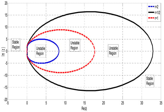
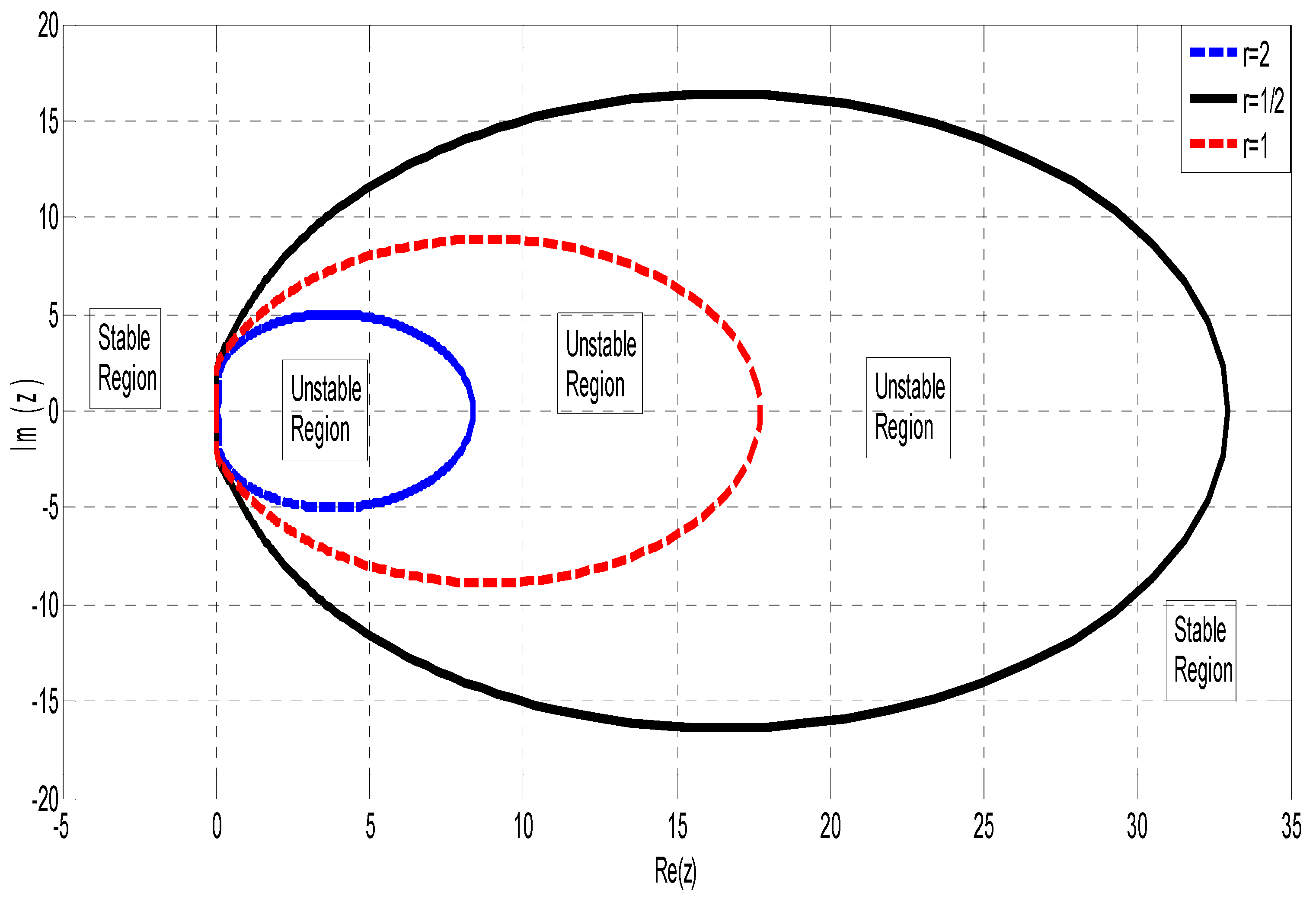
The regions of absolute stability of the TSA are shown in Figure 2.
Figure 2.
Region of absolute stability of the TSA.
The exterior regions of the blue-, red-, and black-colored contours for , , and , respectively, are the regions of absolute stability of the TSA. Therefore, the TSA for , which corresponds to halving the step size, has the largest region of absolute stability, followed by the TSA for , which corresponds to maintaining the step size. The TSA for is computed, and when the step size is doubled, the TSA yields the smallest absolute stability region. The TSA is therefore A-stable; refer to Definition 4. The intervals of instability of the TSA are presented in Table 2.
Table 2.
On the intervals of instability of the TSA.
The data given in Table 2 clearly show that the computed TSA for obtained or generated has the smallest interval of instability (this means that it is characterized by the widest region of stability). On the other hand, the TSA for exhibits the largest interval of instability, which consequently implies the smallest interval of stability.
4. Algorithm for Implementation of the TSA
The TSA formulated in adaptive/variable step-size mode adjusts the step size dynamically in order to handle the oscillation and excitation of the FHNE, control local truncation error (LTE), and improve accuracy as well as enhance efficiency. The Algorithm 1 has the following steps:
| Algorithm 1: Implementation steps of the TSA |
| Step 1: Initialization In this step, the FHNE is clearly defined, the initial condition is chosen, the initial step is set, the tolerance for error control is defined, the maximum and minimum allowable step size are set, and the maximum number of iteration is defined. Step 2: TSA Predictor Step Here, the predicted value is computed using the explicit predictor TSA. The predicted value of the derivative is also calculated. Step 3: TSA Corrector Step The corrected value is calculated using the formulated implicit corrector TSA. Step 4: Estimation of Error The LTE is estimated. Step 5: Adjustment of Step Size
The process is repeated until the final time is reached or the maximum number of iterations is exceeded. Step 8: Output Return the computed values and for all time steps. |
4.1. Adaptive Step-Size Control Mechanism
This section explicitly describes how the TSA achieves automatic step-size adjustment within the integration interval. The adaptive component allows TSA to automatically refine or enlarge the step length depending on the local solution behavior, improving efficiency while preserving accuracy.
4.1.1. Local Truncation Error Estimation
The TSA incorporates an adaptive step-size mechanism based on the difference between the predictor and corrector approximations. The LTE is estimated using predictor–corrector difference:
where
- or B denotes the predictor value computed from the explicit TSA predictor formulae (Equations (17)–(21));
- or A denotes the corrector value computed from the implicit TSA corrector formulae (Equations (12)–(16)), and = D, and = E
The infinity norm is used to ensure all spatial points satisfy the tolerance. This difference provides a reliable estimate of the local error without requiring additional function evaluations, making the approach computationally efficient.
4.1.2. Step-Size Update Rule
The new step size is computed using the standard adaptive formula:
where
- γ = 0.8 is a safety factor to prevent aggressive oscillations in the step size and excessive step-size changes;
- Tol is the user-specified error tolerance (typically 10−6 to 10−12);
- p = 7 is the order of accuracy of the TSA (proven in Proposition 1);
- hold is the current step size.
The exponent 1/(p + 1) = 1/8 ensures that the step-size adjustment is proportional to the error in a theoretically optimal manner for seventh-order methods.
4.1.3. Adaptive Decision Logic
The step-size adaptation follows this logic at each integration step:
Case 1: Step Acceptance (LTE ≤ Tol)—when Tol, the step is accepted:
- Accept the current step;
- Update solution: and tn ← tn + h;
- Store solution in output array;
- Compute new step size: h ← min(hnew, hmax);
- Select appropriate step-size ratio based on error magnitude:
- If Tol: use r = 2 (double step size for efficiency in smooth regions)
- Otherwise, use r = 1 (maintain step size for stability).
Case 2: Step Rejection ( Tol)
Otherwise, it is rejected and recomputed using a reduced step size:
- Reject the current step (do not update yn or tn).
- Do not store in the output array;
- Reduce step size: h ← max(hnew, hmin);
- Select ratio: r = 1/2 (halve step size for better accuracy in stiff regions);
- Recompute the step with the reduced step size.
4.1.4. Step-Size Ratio Selection
The TSA uses three predefined step-size ratios corresponding to the three sets of formulae derived in Section 2.2:
Each ratio serves a specific purpose:
- r = 1: Maintain current step size (used during stable convergence);
- r = 2: Double step size (used in smooth regions to improve computational efficiency);
- r = 1/2: Halve step size (used in stiff or rapidly varying regions to ensure stability and accuracy).
This discrete ratio approach maintains computational efficiency while providing adequate adaptivity. The specific choice of these three ratios ensures
- Zero-stability is preserved for all ratios (proven in Proposition 2 and Table 1);
- The number of embedded formulae remains manageable (15 total: 5 for each ratio);
- Computational overhead is minimized (no arbitrary ratio calculations needed);
- Code implementation remains efficient (direct formula selection via lookup).
4.1.5. Step-Size Bounds
To ensure numerical stability and computational efficiency, the step size is always constrained within prescribed bounds:
hmin ≤ h ≤ hmax
Typical values used in our implementation:
- hmin = 10−6: Prevents infinitesimally small steps that would cause excessive computation and potential underflow;
- hmax = 0.1: Prevents excessively large steps that could cause numerical instability or miss rapid solution changes.
These bounds are problem-dependent and can be adjusted based on the following:
- The stiffness ratio of the problem (larger ε may require smaller hmax);
- The temporal domain [0, T] (longer intervals may permit larger hmax);
- Desired accuracy (tighter tolerances may require smaller hmin).
4.2. Implementation Strategy and Computational Cost
While TSA corrector formulae are formally implicit, practical implementation employs a Predictor–Corrector (PEC) structure avoiding full Newton iterations.
4.2.1. Predictor–Corrector Structure
TSA uses PEC(k) mode with k = 2 iterations:
- Explicit predictor provides initial values yn(p);
- Implicit corrector applied twice using previous iterate;
- No full implicit solve required per step.
For FHNE problems tested, two iterations maintained
- Seventh-order accuracy;
- Stability consistent with A-stable region (Figure 2);
- Error control within tolerance.
4.2.2. Jacobian Handling
MOL discretization produces tridiagonal structure:
- Jacobian is tridiagonal (bandwidth = 3);
- Only three nonzero entries per row;
- Finite difference evaluation on tridiagonal structure only;
- Sparse storage used (not N × N dense);
- No full matrix inversion performed;
- Jacobian reused across steps when h constant;
- Recomputed only when:
- -
- Step size changes
- -
- Convergence slows
- -
- Step rejected.
4.2.3. Cost Analysis
Per time step:
- Predictor: O(M) (explicit);
- Corrector (2 iterations): 2 × O(M);
- Tridiagonal solve (if needed): O(M) (Thomas algorithm);
- Total: O(M), not O(M2) or O(M3).
Comparison:
- Standard implicit BDF: O(M3) per step (LU factorization);
- TSA with PEC: O(M) per step.
Table 3.
Juxtaposition of for Problem 1 at including CPU time of TSA.
Table 4.
Juxtaposition of and for Problem 2 at including CPU time of TSA.
Table 5.
Juxtaposition of and for Problem 3 at including CPU time of TSA.
4.2.4. Theory-Implementation Coherence
- Theoretical A-stability applies to fully converged implicit corrector;
- PEC with k = 2 achieves stability consistent with theory;
- Verified by numerical results: no instabilities observed, seventh-order convergence confirmed.
5. Results
In order to test the efficiency as well as accuracy of the proposed TSA, three special cases of FHNE shall be examined. The implementation of the new algorithm was done using MATLAB software. Its accuracy was examined in terms of maximum error denoted by and root mean square error denoted by . The results of some existing methods were compared with those of the newly formulated TSA in order to test the accuracy of the later. The following acronyms and notations were adopted in Table 3, Table 4 and Table 5 and Figure 3, Figure 4, Figure 5, Figure 6 and Figure 7:
—time step (evaluation point);
—space variable;
—step size;
CPUT—central processing unit time (in seconds);
SCSCM—shifted Chebyshev spectral collocation method by [13];
CFDBM—coupled finite difference block method by [5];
TSHBM—two-step hybrid block method by [24];
OHBCBM—optimized hybrid block method with cubic B-spline method by [18];
TSA—newly formulated three-step algorithm.
Note that
where denotes the exact solution and denotes the numerical solution generated by the TSA at discrete space point and specific time point .
Figure 3.
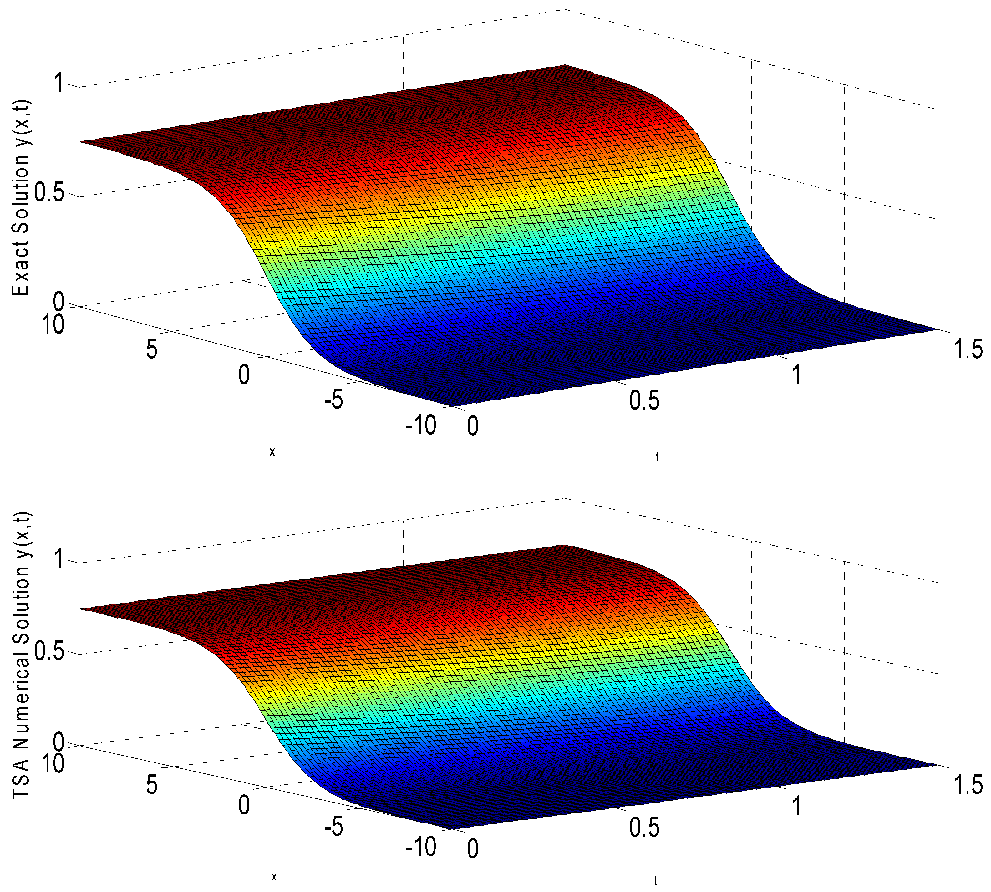
Exact (top) and TSA numerical (bottom) solution curves for Problem 1 at .
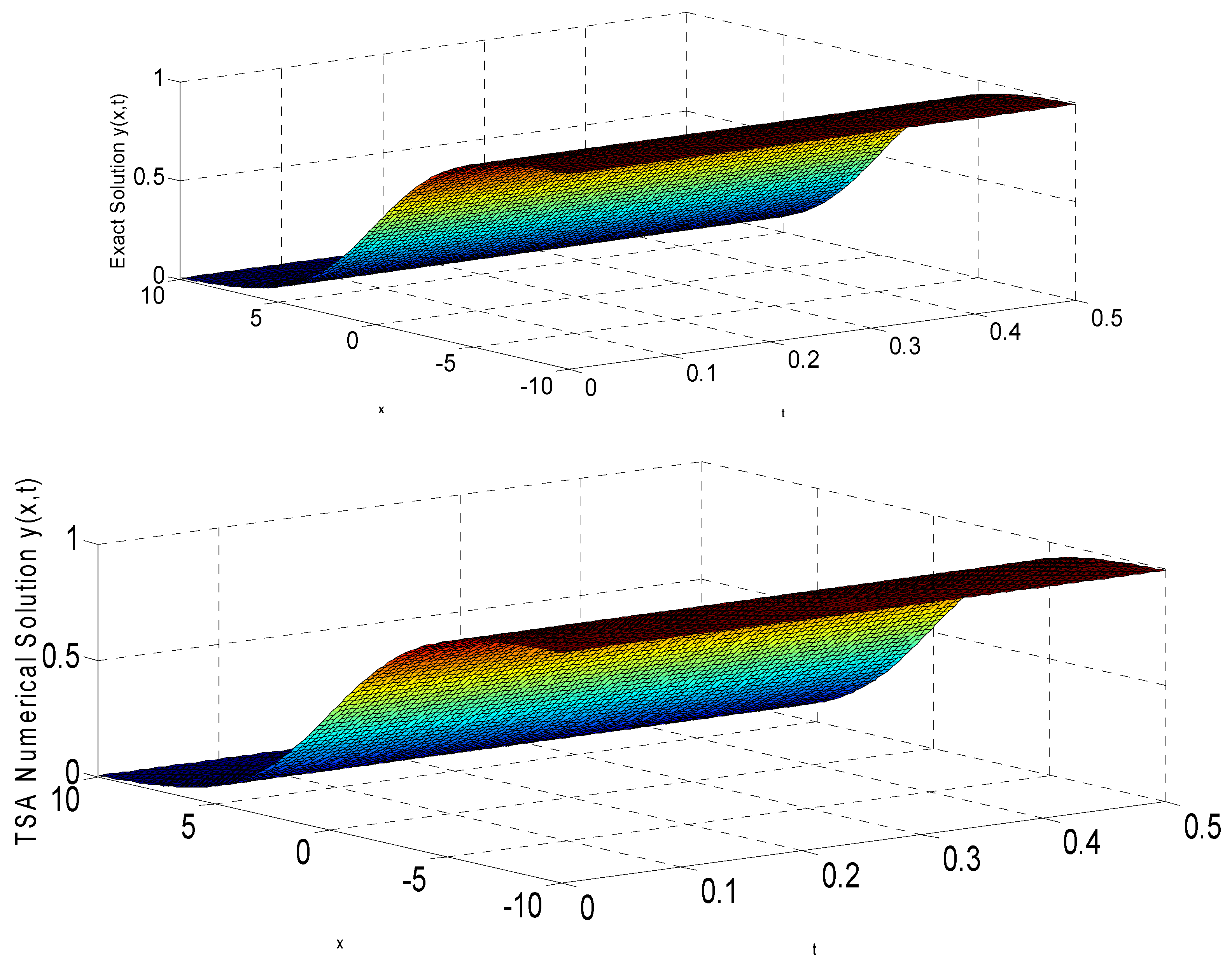
Figure 4.
Exact (top) and TSA numerical (bottom) solution curves for Problem 1 at .
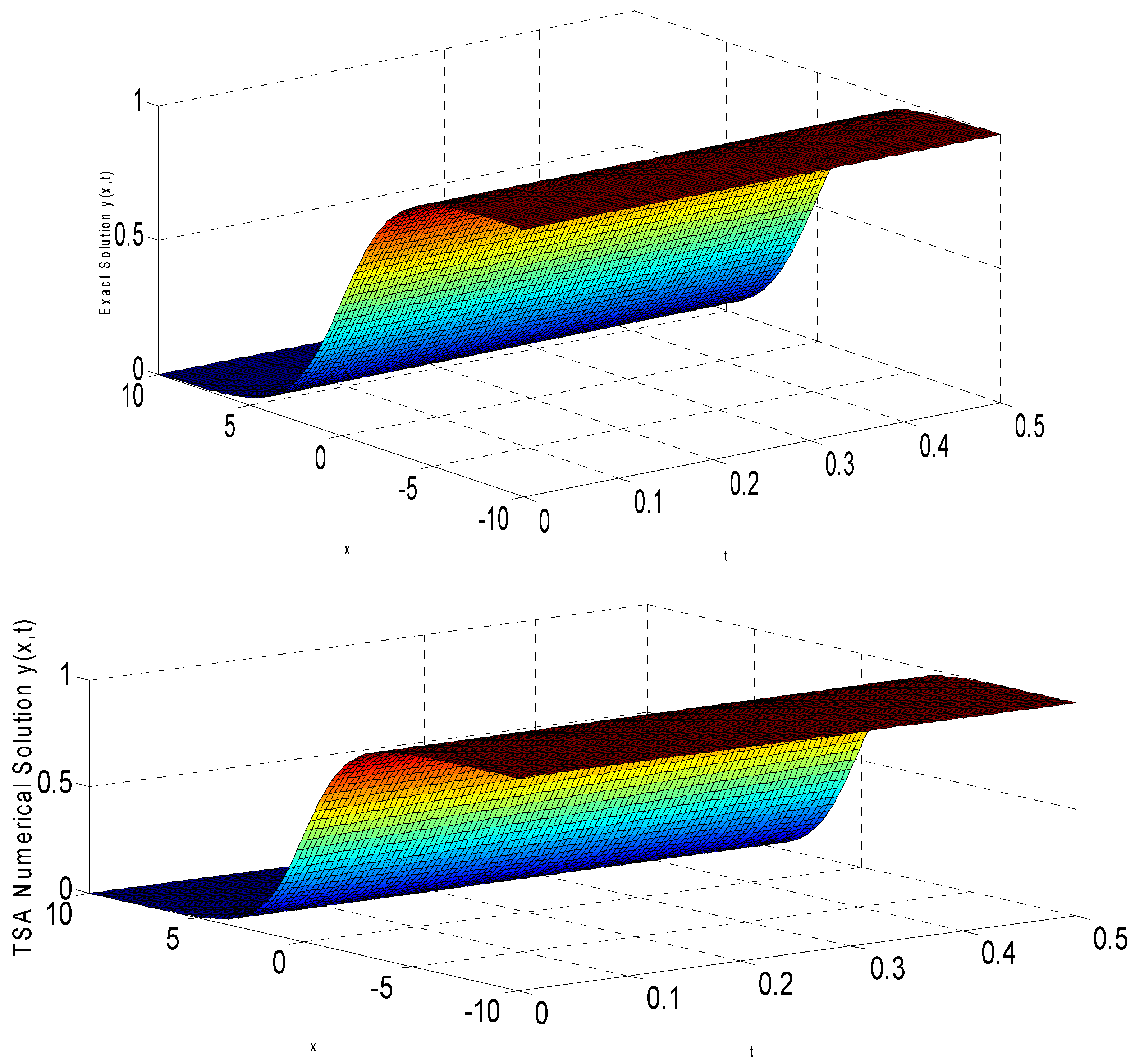
Figure 5.
Exact (top) and TSA numerical (bottom) solution curves for Problem 1 at .
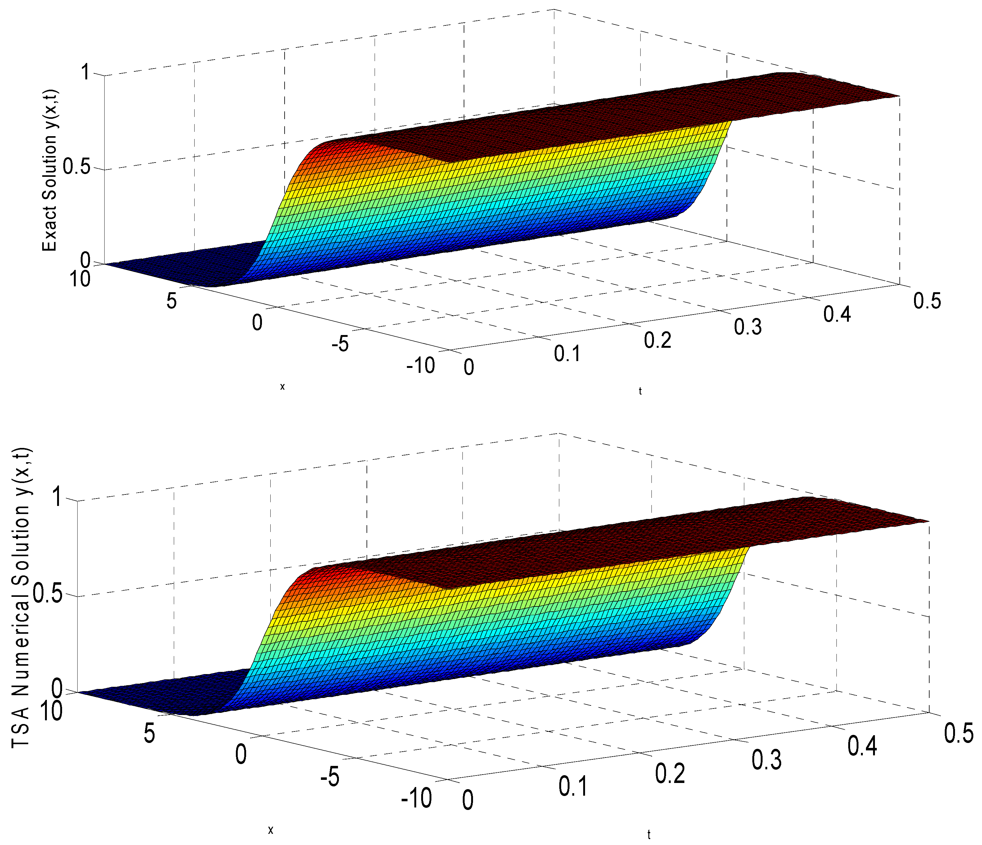
Figure 6.
Exact (top) and TSA numerical (bottom) solution curves for Problem 2.
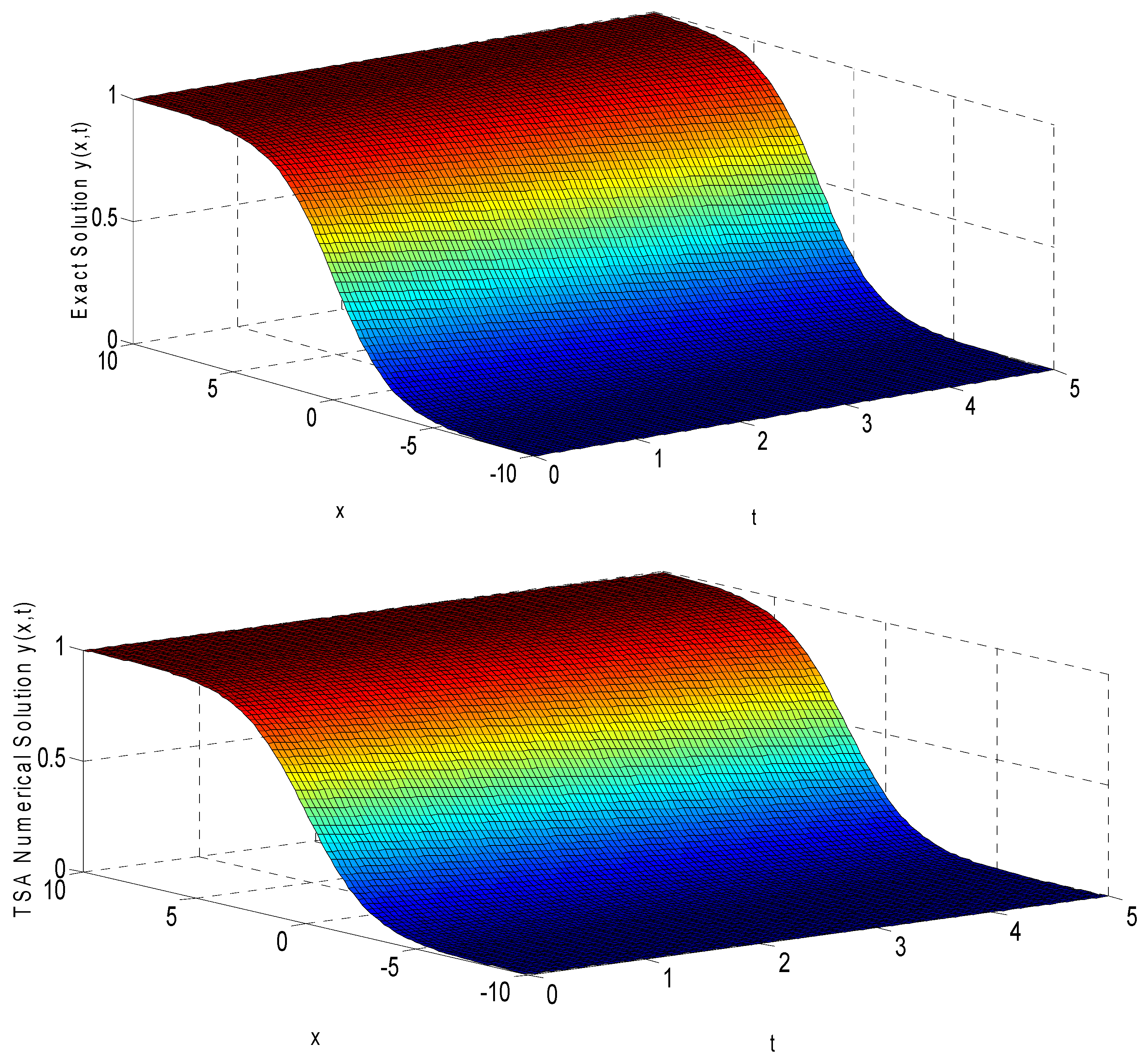
Figure 7.
Exact (top) and TSA numerical (bottom) solution curves for Problem 3.
5.1. Characteristics of Comparison Methods
TSA achieves both higher-order and adaptive control, explaining superior performance.
5.1.1. Comparative Analysis: Order and Adaptivity TSA’s Superior Performance Arises from
- Higher Order:
- TSA: p = 7, error ∼ O(h8);
- CFDBM/TSHBM/OHBCBM: p = 4, 5, 6;
- At h = 0.01: seventh-order ≈ 10−16 vs. fourth-order ≈ 10−10.
- 2.
- Adaptive Step Size:
- TSA adjusts h automatically; • Fixed methods require globally small h;
- Problem 1, ε = 2.0:
- -
- Fixed: h = 10−4 globally (10,000 steps);
- -
- TSA: adaptively (2100 steps);
- -
- Result: 4.8 fewer steps with higher accuracy.
- 3.
- Work-Unit Analysis:
Work units = (steps) × (function evals/step) Problem 1, ε = 2.0:
- CFDBM: 10,000 × 4 = 40,000 units;
- TSHBM: 10,000 × 5 = 50,000 units;
- TSA: 2100 × 7 = 14,700 units.
TSA achieves 2.7–3.4 computational savings with two–three orders of magnitude better accuracy.
5.1.2. Computational Environment and Grid Specifications Hardware/Software
- Processor: Intel Core i7-11700K @ 3.6 GHz (8 cores);
- RAM: 32 GB DDR4;
- OS: Windows 11 Pro (64-bit);
- MATLAB: R2023a (9.14.0.2206163).
Problem 1:
- Spatial: M = 100 points, ∆x = 0.01;
- Initial h0 = 0.01, Tol = 10−10;
- TSA steps:
- -
- ε = 0.5: 87 steps (53 accepted, 34 with r = 2);
- -
- ε = 1.0: 156 steps (124 accepted, 32 with r = 1/2);
- -
- ε = 2.0: 312 steps (289 accepted, 148 with r = 1/2).
Problem 2:
- Spatial: M = 80 points, ∆x = 0.0125;
- Initial h0 = 0.01, Tol = 10−12;
- Steps: 45 (T = 0.2) to 634 (T = 5.0).
Problem 3:
- Spatial: M = 50 points, ∆x = 0.02;
- Initial h0 = 0.005, Tol = 10−10;
- Steps: 67 (T = 0.2) to 412 (T = 1.5).
CPU Time Measurement:
- MATLAB tic/toc for wall-clock time;
- Each problem run 10 times, median reported;
- Includes function evals, PEC iterations, error estimation, storage;
- Excludes setup, post-processing, graphics.
Low CPU times reflect: O(M) cost/step, adaptive step reduction, vector operations, Jacobian reuse.
5.2. Numerical Experiments
Problem 1.
Consider the stiff generalized FHNE (3) with parameters and , for , as reported in [5,24]. The problem is expressed as
where denotes the natural growth rate while the equation’s overall dynamics are characterized by the parameter. The problem is subject to initial condition
and boundary conditions
The exact solution is
where . Suffice to mention that on using (38), the boundary conditions of Problem 1 can be determined.
According to [24], Problem 1 is stiff in nature and tedious to solve because of the presence of slowly varying and rapidly varying components. Also, according to [5], the problem becomes stiff for large value of . The results of discretized Problem 1 shall be presented at three selected values of for and ; see Table 3. The results are presented by comparing the of TSA with those of TSHBM in [24] and CFDBM in [5]. Figure 3, Figure 4 and Figure 5 also show the solution curve for the exact and numerical solutions at the three values of , that is and
Problem 2.
Consider the generalized FHNE (3) with parameters in the domain , reported in [18]. The FHNE is given as
subject to initial condition
and boundary conditions
where . The boundary conditions which are obtained from the analytical solution ensure that the solution remains bounded and also well behaved as the number of time steps are increased [24]. The exact solution is given by
The results of discretized Problem 2 shall be presented at different values of for , and . The numerical results are presented in Table 4 by juxtaposing the and errors of TSA with that of the OHBCBM in [18]. The solution curves in terms of exact and numerical solutions are presented in Figure 6.
Problem 3.
Consider the generalized FHNE (3) with parameters and as reported in [13]. That is,
subject to initial condition
and boundary conditions
where . The exact solution is
5.3. Discussions
The juxtaposition of for Problem 1 at with and at distinct values of is presented in Table 3. The results so obtained clearly showed that the TSA performs better than the CFDMB developed by [5] and TSHBM developed by [24] for the three cases of , that is , , and . These results also show that an increase in the value of implies an increase in the stiffness profile of the problem. The TSA is obviously efficient because it preserves cost effectiveness in terms of computer time by virtue of the CPUT obtained in Table 3. Figure 3, Figure 4 and Figure 5 depict the exact and TSA numerical solutions of Problem 1 for , , and for the three cases of . The accuracy of the TSA is further validated because the solution curves of the exact solution and those of the TSA (numerical solution) are almost the same.
In a bid to compute and , the TSA was also applied to solve Problem 2 at , , and . The results generated in Table 4 validate the fact that the TSA outperformed the OHBCBM derived by [18] at different time levels for . It was observed that as increases, both and also increases. The CPUT taken for the integration of the problem also shows that the TSA is computationally efficient. It is also clear from Figure 6 that the solution curve obtained using the TSA converges to that of the exact solution. This further buttresses the accuracy of the TSA.
Problem 3 was also solved in terms of using the TSA at different time levels by taking , , and . The results obtained show that the TSA performed better than the SCSCM derived by [13]; see Table 5. The evaluation time (in seconds) showed that the TSA is efficient in terms of computer time. In Table 6, the comparison of the properties of the proposed TSA and the existing methods in the cited literatures were showcased. The solution profiles presented in Figure 7 further demonstrate the computational reliability of the TSA, as its solution curve exhibits close agreement with the exact solution. Future research could extend this work by applying the TSA to a broader class of challenging problems, including rigid systems, stiff problems, singular and singularly perturbed problems, as well as integral equations in line with the directions reported in [32,33,34,35].
Table 6.
Comparison of TSA and other existing Methods in the cited Literatures.
6. Conclusions
In this study, a symmetry-compact three-step algorithm (TSA) was developed for the numerical computation of the spatio-temporal generalized FitzHugh–Nagumo equations (FHNE). The proposed algorithm was applied to three representative test cases of the FHNE, and the resulting numerical evidence demonstrated that the symmetry-compact TSA consistently outperformed several existing methods in terms of accuracy and efficiency. The computed solution profiles further confirmed the convergence of the numerical approximations generated by the TSA to the corresponding exact solutions. The reduced execution times observed in the simulations highlight the computational efficiency achieved through the compact and structurally balanced nature of the algorithm. In addition, the rigorous stability and convergence analyses established that the proposed symmetry-compact TSA is A-stable, consistent, and zero-stable, thereby guaranteeing its reliability for long-time integration of stiff spatio-temporal systems. Based on these findings, the study strongly recommends the adoption of the symmetry-compact TSA as an effective and robust numerical tool for obtaining accurate solutions of the FitzHugh-Nagumo equations. Furthermore, the results underscore the potential applicability of the proposed method to a broad range of industrial and scientific problems governed by nonlinear reaction–diffusion equations.
The TSA is fundamentally constructed for semi-discretized systems obtained through the method of lines (MOL). Since MOL applies to two- and three-dimensional PDEs by discretizing each spatial direction independently, the TSA extends naturally to higher dimensions. The only modification required is the treatment of larger, sparse Jacobian structures arising from multidimensional discretization. As TSA operates with banded or sparse system matrices, extension to 2D or 3D domains remains computationally feasible. Future research will focus on implementing TSA for multidimensional FitzHugh–Nagumo-type and reaction–diffusion systems.
Author Contributions
J.S. (software, writing–original draft, conceptualization, methodology, supervision); E.O.O. (methodology, conceptualization, software, analysis, validation); R.B.O. (conceptualization, methodology, investigation); G.M.K. (conceptualization, methodology, analysis); O.O.B. (methodology, analysis, software); O.O.K. (formal analysis, review, and editing). All authors have read and agreed to the published version of the manuscript.
Funding
This research received no external funding.
Data Availability Statement
The original contributions presented in this study are included in the manuscript. Further inquiries can be directed to the corresponding author.
Acknowledgments
The authors thank the anonymous reviewers for their valuable comments and suggestions that greatly improved the manuscript’s clarity and quality.
Conflicts of Interest
The authors declare no conflicts of interest.
Appendix A
Let
Appendix B
Appendix C
and .
Appendix D
and .
References
- FitzHugh, R. Impulses and physiological states in theoretical models of nerve membrane. Biophys. J. 1961, 1, 445. [Google Scholar] [CrossRef] [Scilit] [PubMed]
- Nagumo, J.; Arimoto, S.; Yoshizawa, S. An active pulse transmission line simulating nerve axon. Proc. Inst. Radio Eng. 1962, 50, 2061. [Google Scholar] [CrossRef] [Scilit]
- Cebrián-Lacasa, D.; Parra-Rivas, P.; Ruiz-Reynés, D.; Gelens, L. Six decades of the FitzHugh–Nagumo model: A guide through its spatio-temporal dynamics and influence across disciplines. Phys. Rep. 2024, 1096, 1–39. [Google Scholar] [CrossRef] [Scilit]
- Hodgkin, A.L.; Huxley, A.F. A quantitative description of membrane current and its applications to conduction and excitation in nerve. J. Physiol. 1952, 117, 500. [Google Scholar] [CrossRef] [Scilit]
- Mehta, A.; Singh, G.; Ramos, H. Numerical solution of time dependent nonlinear partial differential equations using a novel block method coupled with compact finite difference scheme. Comput. Appl. Math. 2023, 42, 201. [Google Scholar] [CrossRef] [Scilit]
- Abbasbandy, S. Soliton solutions for the FitzHugh-Nagumo equation with the homotopy analysis. Appl. Math. Model. 2008, 32, 2706. [Google Scholar] [CrossRef] [Scilit]
- Liao, S.J. Homotopy Analysis Method in Nonlinear Differential Equations; Springer: Berlin/Heidelberg, Germany, 2012. [Google Scholar]
- Ali, H.; Kamrujjaman, M.; Islam, M.S. Numerical computation of FitzHugh-Nagumo equation: A novel Galerkin finite element approach. Int. J. Math. Res. 2020, 9, 20. [Google Scholar] [CrossRef] [Scilit]
- Al-Juaifri, G.A.; Harfash, A.J. Finite element analysis of nonlinear reaction-diffusion system of FitzHugh-Nagumo type with Robin boundary conditions. Math. Comput. Simul. 2023, 203, 486. [Google Scholar] [CrossRef] [Scilit]
- Garcia-Olivares, A. Analytic solution of partial differential equations with Adomian decomposition method. Kybernetes 2003, 32, 354. [Google Scholar] [CrossRef] [Scilit]
- Gundogdu, H.; Gozukizil, O.F. Solving nonlinear partial differential equations by using Adomian decomposition method, modified decomposition method and Laplace decomposition method. MANAS J. Eng. 2017, 5, 1–13. [Google Scholar]
- Berestycki, H.; Hamel, F. Spectral methods for the numerical solution of the FitzHugh-Nagumo equation. SIAM J. Numer. Anal. 2021, 59, 1543. [Google Scholar]
- Sharma, S.; Prabhakar, N. Numerical simulation of generalized FitzHugh-Nagumo equation by shifted Chebyshev spectral collocation method. IAENG Int. J. Appl. Math. 2024, 54, 1371. [Google Scholar]
- Hariharan, G.; Kannan, K. Haar wavelet method for solving FitzHugh-Nagumo equation. Int. J. Math. Comput. Sci. 2010, 4, 909. [Google Scholar]
- Feng, H.; Lin, R.A. A finite difference method for the FitzHugh-Nagumo equations. Dyn. Contin. Discret. Impuls Syst. Ser. B Appl. Algorithms 2015, 22, 401. [Google Scholar]
- Xu, D.; Qiu, W.; Guo, J. A compact finite difference scheme for the fourth-order time-fractional integro-differential equation with a weakly singular kernel. Numer. Methods Partial Differ. Equ. 2020, 36, 304. [Google Scholar] [CrossRef] [Scilit]
- Shahid, M.; Abbas, M.; Kwessi, E. Nonstandard nearly exact analysis of the FitzHugh-Nagumo model. Symmetry 2024, 16, 585. [Google Scholar] [CrossRef] [Scilit]
- Ramos, H.; Kaur, A.; Kanwar, V. Using a cubic B-spline method in conjunction with a one-step optimized hybrid block approach to solve nonlinear partial differential equations. Comput. Appl. Math. 2022, 41, 34. [Google Scholar] [CrossRef] [Scilit]
- Inan, B.; Ali, K.K.; Saha, A.; Ak, T. Analytical and numerical solutions of the FitzHugh–Nagumo equation and their multistability behaviour. Numer. Methods Partial. Differ. Equ. 2020, 37, 7–23. [Google Scholar] [CrossRef] [Scilit]
- Raissi, M.; Perdikaris, P.; Karniadakis, G.E. Physics-informed neural networks: A deep learning framework for solving forward and inverse problems involving nonlinear partial differential equations. J. Comput. Phys. 2019, 378, 686. [Google Scholar] [CrossRef] [Scilit]
- Lu, L.; Meng, X.; Mao, Z.; Karniadakis, G.E. DeepXDE: A deep learning library for solving differential equations. SIAM Rev. 2021, 63, 208. [Google Scholar] [CrossRef] [Scilit]
- Zhi, Y.; Wei, X. A hybrid finite element-neural network method for solving the FitzHugh-Nagumo equation. Comput. Methods Appl. Math. 2022, 22, 135. [Google Scholar]
- Fu, E. Dynamics of the FitzHugh-Nagumo equation with numerical methods. Theor. Nat. Sci. 2023, 10, 179–185. [Google Scholar] [CrossRef] [Scilit]
- Rufai, M.I.; Kosti, A.A.; Anastassi, Z.A.; Carpentieri, B. A new two-step hybrid block method for the FitzHugh-Nagumo model equation. Mathematics 2024, 12, 51. [Google Scholar] [CrossRef] [Scilit]
- Krogh, F.T. Algorithms for changing the step size. SIAM J. Num. Anal. 1973, 10, 949. [Google Scholar] [CrossRef] [Scilit]
- Sunday, J.; Shokri, A.; Kwanamu, J.A.; Nonlaopon, K. Numerical integration of stiff differential systems using non-fixed stepsize strategy. Symmetry 2022, 14, 1575. [Google Scholar] [CrossRef] [Scilit]
- Onyekonwu, A.C.; Sunday, J.; Ndam, J.N.; Omole, E.O.; Amoyedo, F.E.; Ajewole, K.P. A multiblock approach to solving fuzzy differential equations with applications. In Proceedings of the IEEE International Conference on Science, Engineering and Business for Driving Sustainable Development Goals, Omu-Aran, Nigeria, 2–4 April 2024. [Google Scholar] [CrossRef] [Scilit]
- Ijam, H.M.; Ibrahim, Z.B.; Zawawi, I.S.M. Stiffly stable diagonally implicit block backward differentiation formula with adaptive step size strategy for stiff ordinary differential equations. MATEMATIKA Malays. J. Ind. Appl. Math. 2024, 40, 27. [Google Scholar]
- Fatunla, S.O. Numerical integrators for stiff and highly oscillatory differential equations. Math Comput. 1980, 34, 373. [Google Scholar] [CrossRef]
- Dahlquist, G.G. A special stability problem for linear multistep methods. BIT Numer. Math. 1963, 3, 27. [Google Scholar] [CrossRef] [Scilit]
- Lambert, J.D. Computational Methods in Ordinary Differential Equations; John Wiley & Sons, Inc.: New York, NY, USA, 1973. [Google Scholar]
- Sunday, J.; Shokri, A.; Kamoh, N.M.; Dang, B.C.; Mahmudov, N.I. A computational approach to solving some applied rigid second-order problems. Math. Comput. Simul. 2024, 217, 121. [Google Scholar] [CrossRef] [Scilit]
- Kamoh, N.M.; Sunday, J.; Soomiyol, C.M. On the performance of Lucas polynomials on linear and nonlinear Volterra integral equations of the second kind. Songklanakarin J. Sci. Technol. 2024, 46, 68. [Google Scholar]
- Sunday, J.; Raymond, D.; Fadugba, S.E.; Omole, E.O.; Shaba, T.G.; Aderemi, E.T. An algorithm for computing problems of singular and singularly perturbed types. In Proceedings of the IEEE International Conference on Science, Engineering and Business for Driving Sustainable Development Goals, Omu-Aran, Nigeria, 2–4 April 2024. [Google Scholar] [CrossRef] [Scilit]
- Sunday, J.; Ndam, J.N.; Kwari, L.J. An accuracy-preserving block hybrid algorithm for the integration of second-order physical systems with oscillatory solutions. J. Niger. Soc. Phys. Sci. 2023, 5, 1017. [Google Scholar] [CrossRef] [Scilit]
- Omole, E.O.; Adeyefa, E.O.; Apanpa, K.I.; Ayodele, V.I.; Amoyedo, F.E.; Emadifar, H. Unveiling the power of an implicit six-point block scheme: Advancing numerical approximation of two-dimensional PDEs in physical systems. PLoS ONE 2024, 19, e0301505. [Google Scholar] [CrossRef] [Scilit]
- Feng, G.; Yu, S.; Wang, T.; Zhang, Z. Discussion on the weak equivalence principle for a Schwarzschild gravitational field based on the light-clock model. Ann. Phys. 2025, 473. [Google Scholar] [CrossRef] [Scilit]
- Xu, X.; Li, B. Semi-global stabilization of parabolic PDE–ODE systems with input saturation. Automatica 2025, 171, 111931. [Google Scholar] [CrossRef] [Scilit]
- Qiao, C.; Long, X.; Yang, L.; Zhu, Y.; Cai, W. Calculation of a dynamical substitute for the real Earth–Moon system based on Hamiltonian analysis. Astrophys. J. 2025, 991, 46. [Google Scholar] [CrossRef] [Scilit]
- Bo, Y.; Tian, D.; Liu, X.; Jin, Y. Discrete maximum principle and energy stability of the compact difference scheme for two-dimensional Allen–Cahn equation. J. Funct. Spaces 2022, 2022, 8522231. [Google Scholar] [CrossRef] [Scilit]
- Huang, Z.; Zheng, X.; Tan, E.L.; Chen, Z.; Shi, L.; Chen, B. Piecewise calculation scheme for the unconditionally stable Chebyshev finite-difference time-domain method. IEEE Trans. Microw. Theory Tech. 2025, 73, 4588–4596. [Google Scholar] [CrossRef] [Scilit]
- Wang, A.; Cheng, C.; Wang, L. On r-invertible matrices over antirings. Publ. Math. Debr. 2025, 106, 445–459. [Google Scholar] [CrossRef] [Scilit]
- Hu, B.; Liao, Y. Convergence conditions for extreme solutions of an impulsive differential system. AIMS Math. 2025, 10, 10591–10604. [Google Scholar] [CrossRef] [Scilit]
- Zhang, B.; Cai, X.; Li, G.; Li, X.; Peng, M.; Yang, M. A modified Algorithm for path planning in the radioactive environment of nuclear facilities. Ann. Nucl. Energy 2025, 214, 111233. [Google Scholar] [CrossRef] [Scilit]
- Cao, S.; Jin, J.; Zhang, D.; Chen, C. A review of Zeroing neural network: Theory, algorithm and application. Neurocomputing 2025, 643, 130425. [Google Scholar] [CrossRef] [Scilit]
- Jin, J.; Zhu, J.; Zhou, L.; Chen, C.; Wu, L.; Lu, M.; Li, Z. A complex-valued variant-parameter robust Zeroing neural network model and its applications. IEEE Trans. Emerg. Top. Comput. Intell. 2024, 8, 1303–1321. [Google Scholar] [CrossRef] [Scilit]
- Kumar, M.D.; Raju, C.S.K.; Shah, N.A.; Yook, S.J.; Gurram, D. Support vector machine learning classification of heat transfer rate in tri-hybrid nanofluid over a 3D stretching surface with suction effects for water at 10 °C and 50 °C. Alex. Eng. J. 2025, 118, 556–578. [Google Scholar] [CrossRef] [Scilit]
- Raza, Q.; Li, S.; Wang, X.; Ali, B.; Shah, N.A. Finite element analysis of morphological effects and nanolayer thermal conductivity in Boger nanofluids under thermal radiation. Chaos Solitons Fractals 2025, 199, 116644. [Google Scholar] [CrossRef] [Scilit]

Disclaimer/Publisher’s Note: The statements, opinions and data contained in all publications are solely those of the individual author(s) and contributor(s) and not of MDPI and/or the editor(s). MDPI and/or the editor(s) disclaim responsibility for any injury to people or property resulting from any ideas, methods, instructions or products referred to in the content. |
© 2026 by the authors. Licensee MDPI, Basel, Switzerland. This article is an open access article distributed under the terms and conditions of the Creative Commons Attribution (CC BY) license.